stress testing engineering: the real risk measurement?

HAL Id: halshs-00951593https://halshs.archives-ouvertes.fr/halshs-00951593

Submitted on 25 Feb 2014

HAL is a multi-disciplinary open accessarchive for the deposit and dissemination of sci-entific research documents, whether they are pub-lished or not. The documents may come fromteaching and research institutions in France orabroad, or from public or private research centers.

L’archive ouverte pluridisciplinaire HAL, estdestinée au dépôt et à la diffusion de documentsscientifiques de niveau recherche, publiés ou non,émanant des établissements d’enseignement et derecherche français ou étrangers, des laboratoirespublics ou privés.

Stress Testing Engineering: the real risk measurement?Dominique Guegan, Bertrand Hassani

To cite this version:Dominique Guegan, Bertrand Hassani. Stress Testing Engineering: the real risk measurement?. 2014.�halshs-00951593�

https://halshs.archives-ouvertes.fr/halshs-00951593

https://hal.archives-ouvertes.fr

Documents de Travail du

Centre d’Economie de la Sorbonne

Stress Testing Engineering: the real risk measurement?

Dominique GUEGAN, Bertrand K. HASSANI

2014.06

Maison des Sciences Économiques, 106-112 boulevard de L'Hôpital, 75647 Paris Cedex 13 http://centredeconomiesorbonne.univ-paris1.fr/bandeau-haut/documents-de-travail/

ISSN : 1955-611X

Stress Testing Engineering: the real risk measurement?

February 6, 2014

• Pr. Dr. Dominique Guégan: Université Paris 1 Panthéon-Sorbonne and NYU - Poly, New

York, CES UMR 8174, 106 boulevard de l’Hopital 75647 Paris Cedex 13, France, phone:

+33144078298, e-mail: [email protected].

• Dr. Bertrand K. Hassani: Université Paris 1 Panthéon-Sorbonne CES UMR 8174 and

Grupo Santander, 106 boulevard de l’Hopital 75647 Paris Cedex 13, France, phone: +44

(0)2070860973, e-mail: [email protected].

Abstract

Stress testing is used to determine the stability or the resilience of a given financial insti-

tution by deliberately submitting the subject to intense and particularly adverse conditions

which has not been considered a priori. This exercise does not imply that the entity’s failure

is imminent, though its purpose is to address and prepare this potential failure. Conse-

quently, as the focal point is a concept (Risk) the stress testing is the quintessence of risk

management. In this chapter we focus on what may lead a bank to fail and how its resilience

can be measured. Two families of triggers are analysed: the first stands in the impact of

external (and/or extreme) events, the second one stands on the impacts of the choice of

inadequate models for predictions or risks measurement; more precisely on models becoming

inadequate with time because of not being sufficiently flexible to adapt themselves to dy-

namical changes. The first trigger needs to take into account fundamental macro-economic

data or massive operational risks while the second trigger deals with the limitations of the

quantitative models for forecasting, pricing, evaluating capital or managing the risks. It

may be argued that if - inside the banks - limitations, pitfalls and other drawbacks of mod-

els used were correctly identified, understood and handled, and if the associated products

were correctly known, priced and insured, then the effects of the crisis may not have had so

important impacts on the real economy. In other words, the appropriate model should be

1

Documents de Travail du Centre d'Economie de la Sorbonne - 2014.06

able to capture real risks (including in particular extreme events) at any point in time, or

ultimately a model management strategy should be considered to switch from a model to

another during extreme market conditions.

1 Introduction

Stress testing (Berkowitz (1999), Quagliariello (2009), Siddique and Hasan (2013)) is used to

determine the stability or the resilience of a given financial institution by deliberately submitting

the subject to intense and particularly adverse conditions which has not been considered a priori.

This involves testing beyond the traditional capabilities - usually to determine limits - to confirm

that intended specifications are both accurate and being met in order to understand the process

underlying failures. This exercise does not mean that the entity’s failure is imminent, though

its purpose is to address and prepare this potential failure. Consequently the stress testing is

the quintessence of risk management.

Since the 1990’s most financial institutions have conducted stress testing exercises on their bal-

ance sheet, but it is only in 2007 following the current crisis, that regulatory institutions became

interested in analyzing and measuring the resilience of financial institutions1 in case of dramatic

movements of economic fundamentals such as the GDP. Then, stress tests have been regularly

performed by regulators to insure that banks are properly adopting practices and strategies which

decrease the chance of a bank failing, in turn jeopardising the entire economy (Berkowitz (1999)).

Originally governments and regulators were keen on measuring financial institutions’ resilience -

and by extension the entire system - in order to avoid future failure that ultimately the tax payer

would have to support. The stress testing framework engenders the following questions: if a risk

is identified even with the smallest probability of occurrence why is it not directly integrated

in the traditional risk models? Why should we have two processes addressing the same risks,

the first under “normal” conditions and the second under stressed condition knowing that the

risk universe combine them? Therefore, are the stress tests really discussing the impact of an

exogenous event on a balance sheet or of an endogenous failing process, for instance when a

1In October 2012, U.S. regulators unveiled new rules expanding this practice by requiring the largest American

banks to undergo stress tests twice per year, once internally and once conducted by the regulators.

2


model is unable to capture certain risks. In other words is the risk of failing and threatening

the entire system only exogenous?

As the ultimate objective is the protection of the system, a clear definition of the latter is neces-

sary as soon as in the capitalist world banks are the corner stone. Figure 1 exhibits a simplified

version of the banking system used in most developed countries around the globe. It has three

layers, the "real" economy at the bottom, the interbanking market in the middle and the central

bank at the top. Based on this representation if we want to measure the system resilience we

need to identify what may potentially threaten the system. Here, we may reasonably assume

that stress-testing and systemic-risk measurement are ultimately connected. As discussed below

a bank may either fail because of a lack of capital or a lack of liquidity. Regarding this risk of

illiquidity we would like to illustrate how tricky it may be to cope with such a risk. In fact,

a bank balance sheet is fairly simple assets are composed of intangible assets, investments and

lendings while the liabilities are on the top shareholder’s equity and subordinated debt then

comes the wholesale funding and finally clients deposits. By changing the money with a short

duration, such as savings into money with a longer one through lending, a bank is operating

a maturity transformation. This ends up in banks having an unfavorable liquidity position as

they do not have access to the money they lent while the money they owe to customer can be

withdrawn at any time on demand. Through ALM2 banks are managing this mismatch, and we

cannot emphasize enough this point implying that banks are structurally illiquid.

Regarding our simplistic representation of the financial system, figure 1 exhibits four potential

failure spots: (i) The central bank cannot provide any liquidity anymore; (ii) Banks are not

funding each other anymore; (iii) A bank of sensible size is failing; (iv) The banks stop financing

the economy.

Regarding the first point (i), considering that the purpose of a central bank is refinancing loans

provided by commercial banks controlling inflation, unemployment rate, etc. , as soon as this

central bank ceases functioning properly the entire system collapses (uncontrolled inflation, etc.).

This point discusses a model failure and falls beyond the stress-testing exercise. Some examples

2Asset and Liability Management

3


Figure 1: Financial System

may be found in the Argentinian or the Russian central banks failure in the 1990’s. Considering

the second point (ii), if banks are not funding each other then some will face a tremendous lack of

liquidity or confidence intra-bank and may fail (for instance it was the case when banks refused

to help Lehman Brothers the 15th September 2007). In this case we are addressing the way

financial institutions face the risk of illiquidity. On the third point (iii), a bank may fail due to

a lack of capital. Consequently how a bank is supposed to be evaluating its capital requirement

considering the major risks is crucial. In 2008 the insurance company AIG almost failed due to

a lack of capital when most of the CDS they sold had been triggered simultaneously. This is the

backbone of risk management inside a bank. Regarding the last point (iv), and assuming that

ultimately the purpose of banks is to generate a profit financing the real economy it is highly

unlikely that they would do it in case of high stress. A lack of liquidity may lead a bank to

stop funding the economy and by the way may engender corporate and retail defaults. These

defaults in chain may themselves drive the financial institution to bankruptcy. In that latter

case we are clearly discussing the way banks are addressing the credit risk.

4


Whatever the origin of the stress inside the banks a failure causes important damages: bankruptcy,

alteration of confidence on the markets and between the banks, recession in the real economy,

succession of defaults from the enterprises, lack of liquidity and claiming of credits. The global

banking system can be strongly and irreparably disrupted. The idea underlying the stress tests

is to imagine the scenarii illustrating the previous situations to introduce dynamical solutions

which can avoid, at each time any dramatic failures.

In this chapter we focus on what may lead a bank to fail and how its resilience can be measured.

As the system is as strong as its weakest link large enough to trigger a chain reaction, by measur-

ing the resilience of all the banks simultaneously, the resilience of the entire system is assessed.

The right question is what may trigger this chain reaction. Following Lorenz (Lorenz (2010))

we have to capture the butterfly which may engender a twister? In this chapter two families

of triggers are analysed: the first stands in the impact of external (and/or extreme) events, the

second one stands on the impacts of the choice of inadequate models for predictions or risks

measurement; more precisely on models becoming inadequate with time because of not being

sufficiently flexible to adapt themselves to dynamical changes. The first trigger needs to take into

account fundamental macro-economic data or massive operational risks while the second trigger

deals with the limitations of the quantitative models for forecasting, pricing, evaluating capital

or managing the risks. An example of model originating of a system failure was the use of the

Gaussian copula to price CDOs (and CDS) as mis-capturing the intrinsic upper tail dependen-

cies characterizing CDOs tranches correlations mechanically ledding to mis-price and mis-hedge

positions and as a matter of fact producing the experienced cataclysm. It may be argued that if

- inside the banks - limitations, pitfalls and other drawbacks of models used were correctly iden-

tified, understood and handled, and if the associated products were correctly known, priced and

insured, then the effects of the crisis may not have had so important impacts on the real economy.

This chapter is structured as follows. In Section two the stress testing framework is presented.

In the third Section the mathematical tools required to develop the stress testing procedures are

introduced. Finally, in a fourth section we discuss and illustrate integration of the stress-testing

strategy directly into the risk models.

5


2 The stress-testing framework

A stress-testing exercise means choosing scenarii that are costly and rare which can lead to the

financial institution failure, Thus we need to integrate them into a model in order to measure

their impact. The integration process may be a simple linear increasing of parameters to enlarge

the confidence interval of the outcomes, or switch to a more advanced model predicting the po-

tential loss due to an extreme event or a succession of extreme events by implementing various

methodologies allowing the capture of multiple behaviours, or adding exogenous variables.

The objective of this exercise is to strengthen the framework for the risk management by under-

standing extreme exposures, i.e. exposure that may fall beyond the “business as usual” capture

domain of a model. We define the capture domain of a model by its capability to be resilient to

the occurrence of an extreme event, i.e. the pertaining risk measure would not fluctuate or only

in a narrow range of values, or would not breach the selected confidence intervals too many times.

By stressing a value the financial institution naturally acknowledges the fact that their models

and the resulting measurements are reflecting their exposure only up to a certain extent. As a

matter of fact this is due to data sets on which the models are calibrated that are not containing

the entire information or are not adapted to the evolution of the real world. Indeed, the data set

only contains past incidents, and even if crisis outcomes are integrated it does not integrate the

future extreme events which are by definition unknown. In other words, even if the models are

conservative enough to consider eventual Black Swans (Taleb (2010)) the stress-testing enables

envisaging Black Swans with blue eyes and white teeth.

Selecting the appropriate scenario is equivalent to selecting the factors that may have an impact

on the models, (e.g. covariates) and to define the level of stress. These scenarii are supposed

to characterise shocks likely to occur more than what historical observations say: shocks that

have never occurred (stress expected loss), shocks reflecting circumstantial break downs, shocks

reflecting future structural breaks. Mathematically all new categories of shocks entail drawing

from some new factor distribution f∗ which is not equal to the original distribution f charac-

terizing the original data set. Every type of shocks have to include correlations, co-movements

6


and specific events, such as crash, bankrupt, systemic failure, etc.

When scenarii are assessed, practitioners have to check the various outcomes. Are they relevant

for the goal? Are they internally consistent? Are they archetypal? Do they represent relatively

stable outcome situations? The risk managers should identify the extremes of the possible

outcomes of the driving forces and check the dimensions for consistency and plausibility. Almost

three key points should be addressed:

1. The time frame: are the "new" trends compatible within the time frame in question?

2. The internal consistency: do the forces describe uncertainties that can construct probable

scenarii?

3. The stakeholder influence: Is it possible to create reliable scenarii considering a potential

negative influence from the stakeholders?

Now, there are a lot of sources which need to be taken into account inside stress tests. We enu-

merate the risks for which a particular attention must be constantly renewed information must

be continuously updated and potential severe outcome reflected in banks’ internal assessments.

These risks are mainly market, credit, operational and liquidity risks.

Applied to market risk some procedures have traditionally been applied to banks’ trading portfo-

lios by considering multiple states of nature scenarii impacting various risk factors. Traditionally

three kinds of approaches are used, standard scenarii, historical scenarii and worst-case scenarii.

This type of stress testing is probably the simplest and therefore suffers from the limitations

related to over simplicity.

As being the fundamental activity of a bank credit risk stress testing is much wider and has even

been integrated into the capital calculations formulas through the Loss Given Default (LGD)

done by financial institutions. But approaches are not limited to capital calculations as stress

testing is also interesting for more traditional credit risk measure. For example Majnoni et al.

(2001) linked the ratio non-performing loan over total assets to several fundamentals macroeco-

nomic variables such as nominal interest rates, inflation, GDP, etc.; Bunn et al. (2005) measured

the impact of aggregate default rates and LGD evaluation of aggregated write-offs for corporate

7


mortgages and unsecured lendings using standard macroeconomic factors like GDP, unemploy-

ment, interest rates, income gearing and loan to value ratios. This last component may be

particularly judicious in the UK considering the level of interest rate for mortgages sold in the

past few years. Practitioners (Pesola (2007)) argue that unexpected shocks should drive loans

related losses and the state of system, i.e. a more fragile system would worsen the losses. There-

fore factors weakening a financial system should interact in a multiplicative way. Counterparty

credit exposure may either be represented by the “current” exposure, the “expected” exposure

or the “expected positive” exposures. Stressing the exposure distributions would naturally im-

pact the measures based on them, for instance the Credit Value Adjustement (CVA) (Gregory

(2012)) via the expected exposure or the expected loss via the expected positive exposure.

By using extreme scenarii operational risks measurement are naturally stressed. Besides as the

methodologies implemented are expected by the regulator to be conservative, i.e. to provide risk

measures larger than what empirical data or traditional approach would give to practitioners.

However these are not sufficient to provide an accurate representation of the risks over time.

Alternative strategies need to be developed such as those presented in the next section.

Liquidity risk arises from situations in which an entity interested in trading an asset cannot

do it because nobody wants to buy or sell it with respect to the market conditions. Liquidity

risk becomes particularly important to entities which currently hold an asset (or want to held

it) since it affects their capability to trade. Manifestations of liquidity risk are very different

if it comes from price droping to zero. In case an asset’s price falling to zero the market is

saying that the asset is worthless. However if one bank cannot find a counterparty interested in

trading the asset this may only be a problem of market equilibrium, i.e. the participants have

trouble finding each other. This is why liquidity risk is usually found to be higher in emerging or

low-volume markets. Accordingly liquidity risk has to be managed in addition to market, credit

and operational risks. Because of its tendency to compound other exposures it is difficult or

impossible to isolate liquidity risk. Some ALM techniques can be applied to assessing liquidity

risk. A simple test for liquidity risk is to look at future net cash flows on a day-by-day basis

where any day that has a sizeable negative net cash flow is of concern. Such an analysis can be

supplemented with stress testing.

8


In this chapter we only partially deal with the “micro” liquidity risk, i.e. the liquidity of an

asset, by opposition to the “macro” liquidity exposure, i.e. of a financial institution which is

an aggregated measure assuming that it is included in market prices dropping up to a certain

extent which is captured in the market risk measurement. The liquidity position of a financial

institution is measured by the quantity of assets to be sold immediately to face the liquidity

requirements, even considering a haircut, while the price of an asset on the market is illiquid if

there is no demand and its price is actually equal to 0, and consequently the measure should

be forward. As a result considering the previous statement - in the next section - we focus on

methodologies to measure and stress the solvency of financial institutions in relation to market,

credit and operational risks.

3 Tools

In this section some of the tools required to develop stress test strategies are introduced. The

main ingredient which is determinant in our point of view is the information set on which our

work relies. This set is definitively determinant and whatever the methodologies we will use

latter the conclusions cannot be done without referring to this information set. After discussing

the role of the data set we briefly recall the measures of risks which can be used and how they

can be computed. This leads us in a first step to introduce the distributions appearing relevant

to obtained realistic risks measures (from an univariate point of view) and second the notion

of dependence permitting to capture interdependences between the risks in order to properly

evaluate their risk measures in a multivariate framework. Finally the question of dynamics that

should be captured in all strategies of risk management is also discussed.

An a priori which is important to note is that financial data sets are always formed with discrete

time data and they cannot be directly associated to continuous data thus in this chapter the

techniques we present are adapted to this kind of data set.

9


3.1 Data mining

Feeding the scenario analysis and evaluating the potential outcomes lie on the quality of the

information set used. Therefore a data mining process should be undertaken. Data mining is

the computational process of discovering patterns in large data sets. The objective process is to

extract information from a data set, make it understandable and prepare it for further use. In

our case the data mining step is equivalent to a pre-processing exercise. Data mining involves

almost six common classes of tasks (Fayyad et al. (1996)):

1. Anomaly detection – This is the search of events which do not conform to expected pat-

terns. These anomalies are often translated into actionable information.

2. Dependency analysis – The objective is to detect interesting relationships between variables

in databases.

3. Clustering – Cluster analysis consists in the task of creating groupings of similar objects.

4. Classification – The classification consists in generalizing known structure to be applicable

to new data sets.

5. Regression & fittings – This statistical process purpose is to find the appropriate model,

distribution or function which represent the "best" (in a certain sense) fit for the data set.

6. Summarisation – This step purpose is to provide a synthetic representation of the data

set.

These classical techniques are recalled as they could be interesting in certain cases to determine

the sets or subsets on which we should work. They could also be useful to exhibit the main

features of the data before beginning a probabilistic analysis (for the risk measure) or doing a

time series analysis to examine the dynamics which seems the more appropriate for stress testing

purposes.

3.2 Risk measures

Even if at the beginning the risk in the banks was evaluated using the standard deviation applied

to different portfolios the financial industry uses now the quantile-based downside risk measures

including the Value-at-Risk (V aRα for confidence level α) and Expected Shortfall. The V aRα

10


measures the losses that may be expected for a given probability, and corresponds to the quan-

tile of the distribution which characterizes the asset or the type of events for which the risk has

to be measured. Thus, the fit of an adequate distribution to the risk factor is definitively an

important task to obtain a reliable value of the risk. Then, in order to measure the importance

of the losses beyond the VaR percentile and to capture the diversification benefits the expected

shortfall measure has been introduced.

The definitions of these two risks measures are recalled below:

Definition 3.1. Given a confidence level α ∈ (0, 1), the V aRα is the relevant quantile3 of the

loss distribution, V aRα(X) = inf{x | P [X > x] 6 1 − α} = inf{x | FX(x) > α} where X is a

risk factor admitting a loss distribution FX .

Definition 3.2. The Expected Shortfall (ESα) is defined as the average of all losses which are

equal or greater than V aRα :

ESα(X) =1

1 − α

∫ 1

αV aRαdp

The Value at Risk initially used to measure financial institutions market risk was popularised

by Riskmetrics (1993). This measure indicates the maximum probable loss given a confidence

level and a time horizon. The V aRα is sometimes referred as the “unexpected” loss. The ex-

pected shortfall has a number of advantages over the V aRα because it takes into account the

tail risk and fulfills the sub-additive property. It has been widely dealt with in the literature,

for instance in Artzner et al. (1999), Rockafellar and Uryasev (2000; 2002) and Delbaen (2000).

Relationships between V aRα and ESα, for some distributions can be found in this book inside

the chapter of Guégan et al. (2014).

Nevertheless even if the regulators asked to the banks to use the V aRα and recently the ESα to

measure their risks and ultimately provide the capital requirements to avoid bankruptcy these

risk measures are not entirely satisfactory:

• They provide a risk measure for an α which is too restrictive considering the risk associated

to the various financial products;

3V aRα(X) = q1−α = F −1

X (α)

11


• The fit of the distribution functions can be complex or inadequate in particular for the

practitioners who want to follow the guidelines proposed by the regulators (Basel II/III

guidelines). Indeed, in case of the operational risks the suggestions is to fit a GPD which

does not correspond very often to a good fit and whose carrying out can be difficult.

• It may be quite challenging to capture extreme events. Taking into account these events

in modelling the tails of the distributions is determinant.

• Finally all the risks are computed considering unimodal distributions which can be non

realistic in practice.

Recently several extensions have been analysed to overcome these limitations and to propose

new routes for the risk measures. These new techniques are briefly recalled and we suggest the

reader to look at the chapter of Guégan et al. (2014) in this book for more details, developments

and applications:

• Following our proposal we suggest the practitioners to use several α to obtain a spectrum

of their expected shortfall and to visualize the evolution of the ES with respect to these

different values. Then, a unique measure can be provided making a convex combination

of these different ES with appropriate weights. This measure is called spectral measure

(Acerbi and Tasche (2002)).

• In the univariate approach if we want to take into account information contained in the

tails we cannot restrict to the GPD as suggested in the guidelines provided by the regu-

lators. There exist other classes of distributions which are very interesting, for instance

the generalized hyperbolic distribution (Barndorff-Nielsen and Halgreen (1977)), the ex-

treme value distributions including the Gumbel, the Frechet and the Weibull distributions

(Leadbetter (1983)), the α-stable distributions (Taqqu and Samorodnisky (1994)) or the

g-and-h distributions (Huggenberger and Klett (2009)) among others.

• Nevertheless the previous distributions are not always sufficient to properly fit the infor-

mation in the tails and another approach could be to build new distributions shifting the

original distribution on the right or left parts in order to take a different information in

the tails. Wang (2000) proposes such a transformation of the initial distribution which

provides a new symmetrical distribution. Sereda et al. (2010) extend this approach to

12


distinguish the right and left part of the distribution taking into account more extreme

events. The function applied to the initial distribution for shifting is called a distortion

function. This idea is ingenious as the information in the tails is captured in a different

way that using the previous classes of distributions.

• Nevertheless when the distribution is shifted with a function close to the Gaussian one as

in Wang (2000) and Sereda et al. (2010) the shift distribution remains unimodal. Thus

we propose to distort the initial distribution with polynomials of odd degree in order to

create several humps in the distributions. This permits to catch all the information in

the extremes of the distributions, and to introduce a new coherent risk measure ρ(X)

computed under the g ⊗ FX distribution where g is the distortion operator and FX the

initial distribution, thus we get:

ρ(X) = Eg[F −1X (x)|F −1

X (x) > F −1X (δ)]. (3.1)

All these previous risk measures can be included within a stress testing strategy.

3.3 Univariate distributions

This section proposes several alternatives for the fitting of a proper distribution to the infor-

mation set related to a risk (losses, scenarios, etc.). The knowledge of the distributions which

characterises each risk factor is determinant for the computation of the associated measures and

will be also determinant in the case of a stress test. The elliptical domain needs to be left aside

to consider distributions which are asymmetric and leptokurtic like the Generalized Hyperbolic

distributions, Generalized Pareto distributions, or Extreme Value Distributions among others.

Their expressions are recalled in the following.

The Generalized Hyperbolic Distribution (GHD) is a continuous probability distribution defined

as a mixture of an inverse Gaussian distribution and a normal distribution. The density function

associated to the GHD is:

f(x, θ) =(γ/δ)λ

√2πKλ(δγ)

eβ(x−µ) Kλ−1/2(α√

δ2 + (x − µ)2)

(√

δ2 + (x − µ2)/α)1/2−λ, (3.2)

with 0 ≤ |β| < α. This class of distributions is very interesting as it relies on five parameters. If

the shape parameter λ is fixed then several well known distributions can be distinguished:

13


1. λ = 1: hyperbolic distribution

2. λ = −1/2: NIG distribution

3. λ = 1 and ξ → 0: Normal distribution

4. λ = 1 and ξ → 1: Symmetric and asymmetric Laplace distribution

5. λ = 1 and χ → ±ξ: Inverse Gaussian distribution

6. λ = 1 and |χ| → 1: Exponential distribution

7. −∞ < λ < −2: Asymmetric Student

8. −∞ < λ < −2 and β = 0: Symmetric Student

9. γ = 0 and 0 < λ < ∞: Asymmetric Normal Gamma distribution

The four other parameters can be then associated to the first four moments permitting a very

good fit of the distributions to the corresponding losses.

Another class of distributions is the Extreme Value Distributions built on sequences of maxima

obtained from the initial data sets. To introduce this class, the famous Fisher-Tippett theorem

needs to be recalled:

Theorem 3.1. Let be (Xn)a sequence of i.i.d.r.v. If it exists constants cn > 0, dn ∈ IR and a

non degenerated distribution function Gα such that

c−1n (Mn − dn)

L→ Gα (3.3)

then Gα is equal to:

Gα(x) =

exp(−(1 + αx)− 1

α ) α 6= 0, 1 + αx > 0

exp(−e−x) α = 0, x ∈ IR

This function Gα(x) contains several classes of extreme values distributions:

. Fréchet (type III) : Φα(x) = G1/α(x−11/α ) =

0 x ≤ 0

exp(−x−α), x > 0, α > 0

. Weibull (Type II) : Ψα(x) = G−1/α(x+11/α ) =

exp{−(−xα)}, x ≤ 0, α > 0

1

14


. Gumbel (Type I) : Λ(x) = G0(x) = exp(−e−x), x ∈ IR.

Considering only the maxima of a data set is an alternative to model in a robust way the impact

of the extremes of a series within a stress testing strategy.

Another class of distributions permitting to model the extremes is the distribution built on a

data set defined above or under a threshold. Let X a r.v. with distribution function F and right

end point xF and a fixed u < xF . Then,

Fu(x) = P [X − u ≤ x|X > u], x ≥ 0,

is the excess distribution function of the r.v. X (with the df F ) over the threshold u, and the

function

e(u) = E[X − u|X > u]

is called the mean excess function of X which can play a fundamental role in risk management.

The limit of the excess distribution has the distribution Gξ defined by:

Gξ(x) =

1 − (1 + ξx)− 1

ξ ξ 6= 0,

1 − e−x ξ = 0, .

where,

x ≥ 0 ξ ≥ 0,

0 ≤ x ≤ −1ξ ξ < 0, .

The function Gξ(x) is the standard Generalized Pareto Distribution. One can introduce the

related location-scale family Gξ,ν,β(x) by replacing the argument x by (x − ν)/β for ν ∈ IR,

β > 0. The support has to be adjusted accordingly. We refer to Gξ,ν,β(x) as GPD.

Another class of distributions is the class of α-stable distributions defined through their chara-

teristic function also relying on several parameters. For 0 < α ≤ 2, σ > 0, β ∈ [−1, 1] and

µ ∈ R+, Sα(σ, β, µ) denotes the stable distribution with the characteristic exponent (index of

stability) α, the scale parameter σ, the symmetric index (skewness parameter) β and the location

parameter µ. Sα(σ, β, µ) is the distribution of a r.v. X with characteristic function,

E[eixX ] =

exp(iµx − σα|x|α(1 − iβsign(x)tan(πα/2))) α 6= 1,

exp(iµx − σ|x|(1 + (2/π)iβsign(x)ln|x|)) α = 1 ,

15


where x ∈ R, i2 = −1, sign(x) is the sign of x defined by sign(x) = 1 if x > 0, sign(0) = 0

and sign(x) = −1 otherwise. A closed form expression for the density f(x) of the distribution

Sα(σ, β, µ) is available in the following cases: α = 2 (Gaussian distribution), α = 1 and β = 0

(Cauchy distribution) and α = 1/2 and β = +/ − 1 (Levy distributions). The index of stability

α characterises the heaviness of the stable distribution Sα(σ, β, µ).

Finally we introduce the g-and-h random variable Xg,h obtained transforming the standard

normal random variable with the transformation function Tg,h:

Tg,h(y) =

exp(gy)−1g exp(hy2

2 ) g 6= 0,

yexp(hy2

2 ) g = 0, .

Thus

Xg,h = Tg,h(Y ), when Y ∼ N(0, 1).

This transformation allows for asymmetry and heavy tails. The parameter g determines the di-

rection and the amount of asymmetry. A positive value of g corresponds to a positive skewness.

The special symmetric case which is obtained for g = 0 is known as h distribution. For h > 0

the distribution is leptokurtic with the mass is the tails increasing in h.

Thus to model the margins of all items forming a portfolio we have several choices in order to

capture asymmetry, leptokurtosis and extreme events:

• The Generalized Hyperbolic Distribution

• The Extreme Value Distribution Gα, α ∈ IR which describes the limit distributions of

normalised maxima

• The Generalized Pareto Distribution Gξ,β(x), ξ ∈ IR, β > 0 which appears as the limit

distribution of scaled excesses over high thresholds.

• The α-stable distributions

• The g-and-h distributions.

16


Now with respect to the risks we need to measure the estimation and the fitting of the univariate

distributions will be adapted to the data sets. The models will be different depending on the

kind of risks we would like to investigate.

3.4 Interdependence between risks

A necessity of the stress testing is to take into account the interactions or interdependences be-

tween the entities, business units, items or risks. In most of the case, a bank will be associated

to a unique risk portfolio and this one is often modelled as a weighted sum of all its parties. This

approach is very restrictive as even if it captures in a certain sense the correlation between the

lines it is not sufficient to model all the dependences between the risks characterising the bank.

The same observation can be done when we consider the interactions between the different banks

trading by the way the same products. We need to bypass this univariate approach and work

with a multivariate approach. This multivariate approach permits to explain and measure the

contagion effects between all the parties to model the systemic risks and their possible propaga-

tion between the different parties.

A robust way to measure the dependence between large data sets is to compute their joint distri-

bution function. As soon as independence between the assets or risks characterizing the banks

or between the banks cannot be assumed measuring interdependence can be done through the

notion of copula. Recall that a copula is a multivariate distribution function linking a large set

of data through their standard uniform marginal distributions (Bedford and Cooke (2001), Berg

and Aas (2009)). In the literature, it has often been mentioned that the use of copulas is difficult

when we have more than two risks apart from using elliptical copulas such as the Gaussian one

or the Student one (Gourier et al. (2009)). It is now well known that these restrictions can be

released considering recent developments on copulas either using nested copulas (Sklar (1959),

Joe (2005)) or vine copulas (Mendes et al. (2007), Rodriguez (2007), Weiss (2010), Brechmann

et al. (2010), Guégan and Maugis (2010) and Dissmann et al. (2011)). These n-dimensional

copulas need to be fed by some marginal distributions. For instance they can correspond to

distributions characterizing the various risks faced by a financial institution. The calibration of

the exposure distribution plays an important role in the assessment of the risks, whatever the

method used for the dependence structure as discussed in the next section.

17


Until now most practitioners use Gaussian or Student t-copulas however they fail to capture

asymmetric (and extreme) shocks (for example operational risks severity distributions are asym-

metric - sic!). Using a Student t-copula with three degrees of freedom4 to capture a dependence

between the largest losses would mechanically imply a higher correlation between the very small

losses. An alternative is to use Archimedean or Extreme Value copulas (Joe (1997a)) which

have attracted particular interest due to their capability to capture the dependence embedded

in different parts of the marginal distributions (right tail, left tail and body). The mechanism

is recalled in the following.

Let X = [X1, X2, ..., Xn] be a vector of random variables, with joint distribution F and marginal

distributions F1, F2, ..., Fn . Sklar (1959) theorem insures the existence of a function C(.) map-

ping the individual distribution to the joint distribution:

F (x) = C(F1(x1), F2(x2), ..., Fn(xn)).

From any multivariate distribution F , the marginal distributions Fi can be extracted, and also

the copula C. Given any set of marginal distributions (F1, F2, ..., Fn) and any copula C the above

formula can be used to compute the joint distribution with the specified marginals and copula.

The function C can be an Elliptical copula (Gaussian and Student Copulas) or an Archimedean

copulas (defined through a generator) as

C(FX , FY ) = φ−1[φ(FX) + φ(FY )],

including the Gumbel, the Clayton the Franck copulas, among others. The Archimedean copula

are easy to use because of the link existing between the Kendall’s tau and the generator φ:

τ(Cα) = 1 + 4

∫ 1

0

φα(t)

φ′α(t)

dt. (3.4)

If we want to measure the interdependence between more than two risks the Archimedean nested

copula is the most intuitive way to build n-variate copulas with bivariate copulas and consists

in composing copulas together yielding formulas of the following type. For instance when n = 3:

F (x1, x2, x3) = Cθ1,θ2(F (x1), F (x2), F (x3))

= Cθ1(Cθ2

(F (x1), F (x2)), F (x3))

4A low number of degrees of freedom imply a higher dependence in the tail of the marginal distributions

18


where θi, i = 1, 2 is the parameter of the copula. This decomposition can be done several times,

allowing to build copulas of any dimension under specific constraints to insure that it is always a

copula. Therefore a large number of multivariate Archimedean structures have been developed

for instance, the fully nested structures, the partially nested copulas and the hierarchical ones.

Nevertheless all these architectures imply restrictions on the parameters and impose using an

Archimedean copula at each node, making their use limited in practice. To bypass the restric-

tions imposed by the previous nested strategy an intuitive approach proposed by Genest et al.

(1995) can be used based on a pair-copula decomposition such as the D-vine (Joe (1997b)) or the

R-vine (Mendes et al. (2007)). These approaches rewrite the n-density function associated with

the n-copula as a product of conditional marginal and copula densities. All the conditioning

pair densities are built iteratively to obtain the final one representing the entire dependence

structure. The approach is simple and has no restriction for the choice of functions and their

parameters. Its only limitation is the number of decompositions to consider as the number of

vines grows exponentially with the dimension of the data sample and thus requires the user to

select a vine from n!2 possible vines, Capéraà et al. (2000), Galambos (1978), Brechmann et al.

(2010) and Guégan and Maugis (2010; 2011). These are briefly introduced now.

If f denotes the density function associated with the distribution F of a set of n r.v.X, then the

joint n-variate density can be obtained as a product of conditional densities. For instance when

n = 3 the following decomposition is obtained:

f(x1, x2, x3) = f(x1).f(x2|x1).f(x3|x1, x2),

where,

f(x2|x1) = c1,2(F (x1), F (x2)).f(x2),

and c1,2(F (x1), F (x2)) is the density copula associated with the copula C which links the two

margins F (x1) and F (x2). With the same notations we have:

f(x3|x1, x2) = c2,3|1(F (x2|x1), F (x3|x1)).f(x3|x1)

= c2,3|1(F (x2|x1), F (x3|x1)).c1,3(F (x1), F (x3)).f(x3).

19


Then,

f(x1, x2, x3) =f(x1).f(x2).f(x3)

.c1,2(F (x1), F (x2)).c1,3(F (x1), F (x3))

.c2,3|1(F (x2|x1), F (x3|x1)).

(3.5)

Other decompositions are possible using different permutations. These decompositions can be

used whatever the links between the r.v. as there is no constraint. To use it in practice and

eventually to obtain an initial measure of dependence between the risks inside the banks the

first conditioning has to be selected.

3.5 Dynamic approach

In order to take into account events at the origin of stress some banks consider them as single

events by simply summing them thus the complete dependence scheme including their arrival

time is not taken into account; it appears unrealistic as it may lead to both inaccurate capital

charge evaluation and wrong management decisions. In order to overcome the problems created

by these choices we suggest to use the following methodology based on the existence of depen-

dencies between the losses through a time series process.

The dependence between assets, risks, etc. within a bank and with other banks exists and it is

crucial to measure it. We propopse in the previous subsection a way to take them into account.

If it does correctly it can avoid the creation of systemic risks. Nevertheless sometimes this

dependence does not appear and it seems that the independence assumption cannot be rejected a

priori, thus a profound analysis should always be performed at each step of the cognitive process.

Therefore, in order to build a model close to the reality, static models have to be avoided and

intrinsic dynamics should be introduced. The knowledge of this dynamical component should

allow to build robust stress tests. To avoid bankruptcies and failures, generally we focus on the

incidents performing any probabilistic study as proposed in the previous subsections nevertheless

analysing the dynamics embedded within the incidents through time series will permit to be more

reactive and close to the reality. If (Xt)t ∀t denotes the losses, then our objective is to propose

some time series models permitting to link the losses in time. These dynamics can be expressed

20


in the formal following way:

Xt = f(Xt−1,...) + εt, (3.6)

where the function f(.) can take various expressions to model the serial correlations between the

losses, and (εt)t is a strong white noise following any distribution. Various classes of models may

be adopted for instance short memory models e.g. AutoRegressive (AR) processes, GARCH

models or long term models, e.g. Gegenbauer processes.

Besides the famous ARMA model which corresponds to a linear regression of the observations

(losses here) on their known passed values (Brockwell and Davis (1988)) characterising the

fluctuations of the level of the losses it is possible to measure the amplitude of their volatility

using ARCH/GARCH models whose a simple representation is (Engle (1982), Bollerslev (1986)),

Xt|Ft−1 ∼ D(0, ht), (3.7)

where ht can be expressed as:

ht = h(Xt−1, Xt−2, · · · , Xt−p, a), (3.8)

where h(.) is a non linear function in the r.v. Xi, i = 1, ..., p, p is the order of the ARCH process,

a is a vector of unknown parameters, D(.) is any distribution previously introduced, and Ft−1

the σ-algebra generated by the past of the process Xs, for s < t, i.e.: Ft−1 = σ(Xs, s < t).

If we observe both persistence and seasonality inside the losses those can be modelled in the

following way:k

∏

i=1

(I − 2 cos(λi)B + B2)diXt = ut, (3.9)

where k ∈ N , λi are the k frequencies. This representation is called a Gegenbauer process

(Guégan (2005)) and corresponds to the k cycles whose periods are equal to 2π/λi and di are

fractional numbers which measure the persistence inside the cycles. This representation includes

the FARMA processes (Beran (1994)).

Through these time series processes the risks associated to the loss intensity which may increase

during crises or turmoil are captured and the existence of correlations, dynamics inside the

events, and large events will be reflected in the choice of the residual distributions. With this

21


dynamical approach we reinforce the information done by the marginal distribution: for instance

for operational risks using a time series permit to capture the dynamics between the losses and

the adequate choice of the distribution of the filtering data set permits to capture the information

provided in the fat tails.

4 Stress-Testing: A Combined Application

Most stress testing processes in financial institutions begin with negative economic scenarii and

evaluate how the models would react to these shocks. Unfortunately, considering that the stress

testing is supposed to evaluate the resilience of the bank in case of an extreme shock, if the

model used to evaluate how the capital requirements would react to the integration of extreme

information, by definition the model does not fully capture the risks. Obviously, it is not always

simple to fully capture a bank exposure through a model, for two reasons: on the first hand,

financial institutions may follow an adverse selection process, because the more extreme infor-

mation you integrate, the larger the capital charge, and on the other hand the risks may not

have all been identified, and in this case we are going way beyond the Black Swans.

In this section using an alternative economic reality we present approaches that allow to take

into account risk behaviors that may not be captured with traditional strategies. Our objective,

is not to say “the larger the capital charge the better”, but to integrate all the information

left aside by traditional methodologies to understand what would be the appropriate capital

requirement necessary to face a extreme shock up to a certain threshold; as even if we are going

further than traditional strategies to capture multiple patterns usually left aside, our models -

as any model - will have its limitations, but in our case the pros and cons scale inclines toward

the pros. The methodologies presented in the previous sections are applied to Market, Credit

and Operational Risk data. The data used in this analysis are all genuine and the results reli-

able. However, in order not to confuse our message, a fictive financial institution is considered

where its credit risks arise from loans contracted with foreign countries, the market risks from

investments in the French CAC 40 and its operational risks are only characterized by Execution,

Delivery and Process Management failures.

22


The impact of the methodologies are analysed applying four steps approach:

1. In a first step, the risk measures are computed using a traditional but not conservative

approach. The marginal distributions are combined using a Gaussian copula.

2. In a second step, the marginal distributions are built challenging the traditional aspect

either methodologically or with respect to the parameters increasing the conservativeness

of the risk metrics.

3. In a third step, we introduce a dynamical approach.

4. In a fourth step, the dependence architecture is modified to capture the extreme depen-

dencies through a Gumbel copula.

Then, for all steps listed above the impact on the capital requirement and mechanically on both

the risk weight asset (RWA) and the bank balance sheet is illustrated.

4.1 Univariate approach

For each of the three risks (credit, market and operational risks) the objective is to build profit

and loss distributions. Using all data sets three marginal distributions are constructed consid-

ering various type of stress testing to evaluate the buffer a financial institution should hold to

survive to a shock.

4.1.1 Credit Risks

For stressing the credit risk, various options may be considered from the simplest which would

be to shock the parameters of the regulatory approach to the fit of a fat tailed distribution on

the P&L function. The way the parameters are estimated may also be revised. In this section,

three approaches are presented. The first provides a benchmark following the regulatory way to

compute the credit risk capital charge. In the second step, the inputs are changed to reflect an

economical downturn scenario. In a third step a Stable distribution (Taqqu and Samorodnisky

(1994)) is fitted on the P&L distribution to capture extreme shocks.

23


Traditional Scheme The credit risk rating provided by S&P which characterizes the proba-

bility of default of the sovereigns5. Table 2 provides the probabilities of moving from a rating to

another over a year. For credit risk the regulation (BCBS (2006)) provides the following formula

to calculate the capital required:

K = (LGD∗Φ(

√

1

(1 − ρ)∗Φ−1(PD)+

√

ρ

(1 − ρ)∗Φ−1(Q))−PD∗LGD)∗ 1

(1 − 1.5 ∗ b)∗(1+(M−2.5)∗b),

(4.1)

RWA = K ∗ 12.5% ∗ EAD (4.2)

where, the LGD is the Loss Given Default, the EAD is the Exposure At Default, the PD is

the Probability of Default, b = ((0.11852 − 0.05478) ∗ ln(PD))2 (maturity adjustment)6, ρ corre-

sponds to the default correlation, M the number of assets, Φ is the cdf of a Gaussian distribution

and Q represents the 99th percentile.

However, in our case the objective is to build a P&L distribution to measure the risk associated

to the loans provided through the VaR or the Expected Shortfall, and to use it as a marginal

distribution in a multivariate approach. Our approach is not limited to the regulatory capital.

Therefore, a methodology identical to the one proposed by Morgan (1997) has been implemented.

This one is based on Merton’s model (Merton (1972)) which draws a parallel between option

pricing and credit risk evaluation to evaluate the Probabilities of Default.

The portfolio used in this section contains loans to eight countries, for which the bank exposure

is respectively $40, $10, $50, $47, $25, $70, $40, $23 million. The risk free rate is equal to 3%.

The Loss Given Default has been estimated historicaly and is set at 45% and the correlation

matrix is presented in Table 1 and the rating migration matrix in Table 2 (Guégan et al. (2013)).

The VaR and the ES obtained are respectively, $35 380 683 and $40 888 259 (Table 5).

Stressing the input Stressing the input means that the parameters should reflect a crisis

business cycle characterised for example by a decreasing GDP, an increasing unemployment

5http://www.standardandpoors.com/ratings/articles/en/us/?articleType=HTML&assetID=12453501567396The maturity adjustment is not always present as it is contingent to the type of credit.

24


1 0.4 0.6 0.4 0.5 0.3 0.3 0.2

0.4 1 0.5 0.6 0.5 0.4 0.3 0.2

0.6 0.5 1 0.2 0.3 0.2 0.2 0.2

0.4 0.6 0.2 1 0.2 0.2 0.3 0.4

0.5 0.5 0.3 0.2 1 0.4 0.3 0.2

0.3 0.4 0.2 0.2 0.4 1 0.4 0.4

0.3 0.3 0.2 0.3 0.3 0.4 1 0.2

0.2 0.2 0.2 0.4 0.2 0.4 0.2 1

Table 1: Correlation Matrix used to evaluate the Credit Risk regulatory capital.

AAA AA A BBB BB B C D

AAA 92.3 6.9 0.1 0.2 0.5 0.0 0.0 0.0

AA 9.9 82.7 5.0 2.0 0.4 0.0 0.0 0.0

A 0.0 10.8 77.1 9.6 1.7 0.2 0.3 0.3

BBB 0.0 0.0 20.4 69.1 7.2 1.2 0.5 1.6

BB 0.0 0.0 0.0 18.2 67.6 10.4 0.8 3.0

B 0.0 0.0 0.0 0.6 17.1 73.1 2.4 6.8

C 0.0 0.0 0.0 0.0 0.0 32.5 16.6 50.9

D 0 0 0 0 0 0 0 100

Table 2: Probability of Default: Credit Migration Matrix (S&P)

rate, etc. resulting in higher probabilities of default, larger exposures at defaults, higher corre-

lation etc. Considering that during an economical downturn, input data are already stressed,

is extremely risky, as they do not contain the next extreme events. The objective of the stress

testing is to evaluate the resilience of the bank to extreme shocks, where the term extreme char-

acterises events that are worse than what the financial institution already experienced.

The LGD has been stressed from 0.45 to 0.55, and Table 3 provides the stressed ratings migration

matrix. In credit risk management, the simple application of a LGD downturn as prescribed

by the regulation is by itself the integration of stress-testing into the traditional credit risk

25


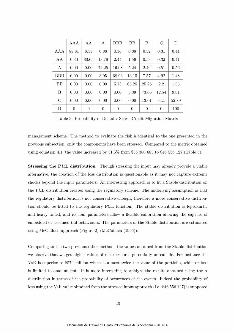
AAA AA A BBB BB B C D

AAA 88.81 8.53 0.88 0.36 0.38 0.32 0.31 0.41

AA 0.30 80.65 13.79 2.44 1.56 0.53 0.32 0.41

A 0.00 0.00 74.25 16.98 5.24 2.46 0.51 0.56

BBB 0.00 0.00 3.95 68.93 13.15 7.57 4.92 1.48

BB 0.00 0.00 0.00 5.73 65.25 25.26 2.2 1.56

B 0.00 0.00 0.00 0.00 5.39 73.06 12.54 9.01

C 0.00 0.00 0.00 0.00 0.00 13.01 34.1 52.89

D 0 0 0 0 0 0 0 100

Table 3: Probability of Default: Stress Credit Migration Matrix

management scheme. The method to evaluate the risk is identical to the one presented in the

previous subsection, only the components have been stressed. Compared to the metric obtained

using equation 4.1, the value increased by 31.5% from $35 380 683 to $46 556 127 (Table 5).

Stressing the P&L distribution Though stressing the input may already provide a viable

alternative, the creation of the loss distribution is questionable as it may not capture extreme

shocks beyond the input parameters. An interesting approach is to fit a Stable distribution on

the P&L distribution created using the regulatory scheme. The underlying assumption is that

the regulatory distribution is not conservative enough, therefore a more conservative distribu-

tion should be fitted to the regulatory P&L function. The stable distribution is leptokurtic

and heavy tailed, and its four parameters allow a flexible calibration allowing the capture of

embedded or assumed tail behaviours. The parameters of the Stable distribution are estimated

using McCulloch approach (Figure 2) (McCulloch (1996)).

Comparing to the two previous other methods the values obtained from the Stable distribution

we observe that we get higher values of risk measures potentially unrealistic. For instance the

VaR is superior to $572 million which is almost twice the value of the portfolio, while or loss

is limited to amount lent. It is more interesting to analyze the results obtained using the α

distribution in terms of the probability of occurences of the events. Indeed the probability of

loss using the VaR value obtained from the stressed input approach (i.e. $46 556 127) is supposed

26


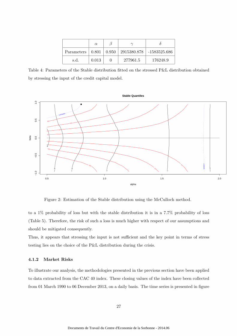
α β γ δ

Parameters 0.801 0.950 2915380.878 -1583525.686

s.d. 0.013 0 277961.5 176248.9

Table 4: Parameters of the Stable distribution fitted on the stressed P&L distribution obtained

by stressing the input of the credit capital model.

alpha

beta

2.5 3 5 1

0

20

40

0.5 1.0 1.5 2.0

−1.

0−

0.5

0.0

0.5

1.0

−0.8

−0.6

−0.4

−0.2

0.2

0.4

0.6 0.8

2.549191

0.8792463

Stable Quantiles

●

Figure 2: Estimation of the Stable distribution using the McCulloch method.

to a 1% probability of loss but with the stable distribution it is in a 7.7% probability of loss

(Table 5). Therefore, the risk of such a loss is much higher with respect of our assumptions and

should be mitigated consequently.

Thus, it appears that stressing the input is not sufficient and the key point in terms of stress

testing lies on the choice of the P&L distribution during the crisis.

4.1.2 Market Risks

To illustrate our analysis, the methodologies presented in the previous section have been applied

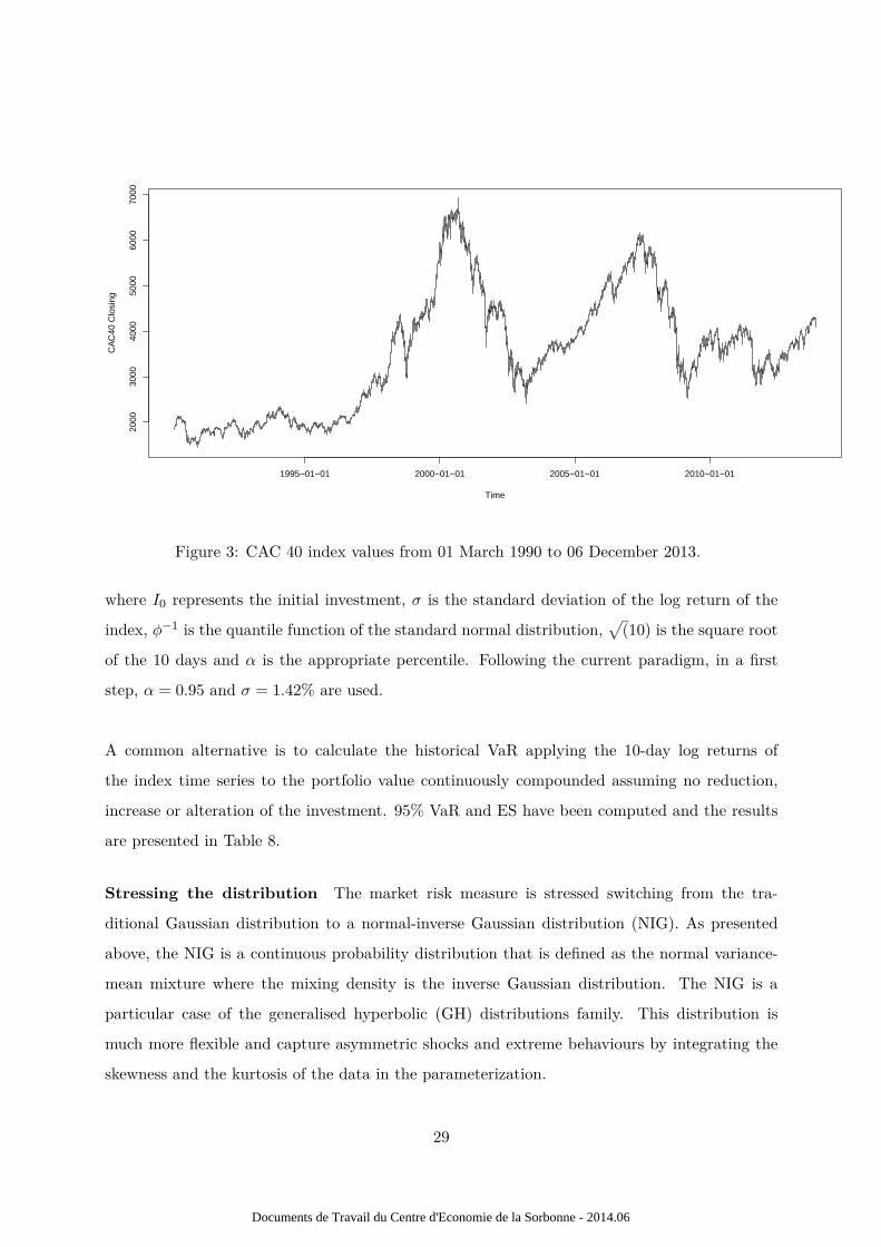
to data extracted from the CAC 40 index. These closing values of the index have been collected

from 01 March 1990 to 06 December 2013, on a daily basis. The time series is presented in figure

27


VaR ES

Regulatory $35 380 683 $40 888 259

Stressed Input $46 556 127 $60 191 821

Stable Distribution $572 798 381 $13 459 805 700

Percentile Equivalent 92.3% NA

Table 5: This table presents the risk measures computed considering the three approaches

presented to model the credit risk, for instance the regulatory approach, the stressed input

approach and the fit of a Stable distribution. The more conservative the approach the larger

the risk measures. Comparing the values obtained from the Stable distribution to the others

exhibits much larger risk measures, potentially unrealistic. Here, we suggest changing the way

the results are read. The line labeled “Percentile Equivalent” provides the probability of losing

the VaR value obtained from the stressed input approach (i.e. $46 556 127) considering a Stable

distribution. What was supposed to be a 1% probability of loss is in fact a 7.7% probability of

loss considering the Stable distribution.

3.

In this subsection, we assume that our fictive financial institution only invested in the assets

constituting the CAC 40 index, in the exact proportion that they replicated the index in such

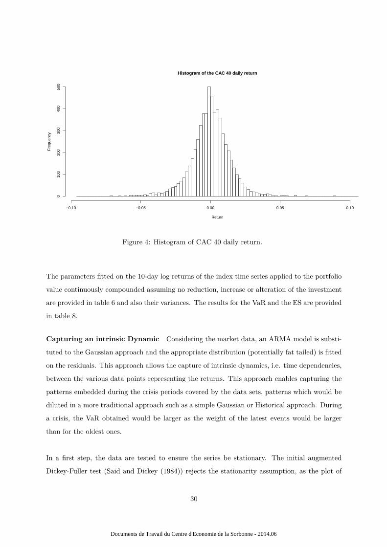
a way that daily returns of their portfolio are identical to those of the CAC 40 index. The

daily return are computed as follows, log( Indext

Indext−1). The histogram of the daily log returns are

represented in figure 4.

In this application, an initial investment of 100 million is considered.

Traditional Scheme Two approaches are considered to build the Profit and Loss distribu-

tions, the Gaussian approximation and the historical log return on investment. In a first step, a

Gaussian distribution is used. The Gaussian VaR is obtained using the following equation,

V aRMarket = I0 ∗ σ ∗ φ−1α (0, 1) ∗

√

(10), (4.3)

28


Time

CA

C40

Clo

sing

1995−01−01 2000−01−01 2005−01−01 2010−01−01

2000

3000

4000

5000

6000

7000

Figure 3: CAC 40 index values from 01 March 1990 to 06 December 2013.

where I0 represents the initial investment, σ is the standard deviation of the log return of the

index, φ−1 is the quantile function of the standard normal distribution,√

(10) is the square root

of the 10 days and α is the appropriate percentile. Following the current paradigm, in a first

step, α = 0.95 and σ = 1.42% are used.

A common alternative is to calculate the historical VaR applying the 10-day log returns of

the index time series to the portfolio value continuously compounded assuming no reduction,

increase or alteration of the investment. 95% VaR and ES have been computed and the results

are presented in Table 8.

Stressing the distribution The market risk measure is stressed switching from the tra-

ditional Gaussian distribution to a normal-inverse Gaussian distribution (NIG). As presented

above, the NIG is a continuous probability distribution that is defined as the normal variance-

mean mixture where the mixing density is the inverse Gaussian distribution. The NIG is a

particular case of the generalised hyperbolic (GH) distributions family. This distribution is

much more flexible and capture asymmetric shocks and extreme behaviours by integrating the

skewness and the kurtosis of the data in the parameterization.

29


Histogram of the CAC 40 daily return

Return

Fre

quen

cy

−0.10 −0.05 0.00 0.05 0.10

010

020

030

040

050

0

Figure 4: Histogram of CAC 40 daily return.

The parameters fitted on the 10-day log returns of the index time series applied to the portfolio

value continuously compounded assuming no reduction, increase or alteration of the investment

are provided in table 6 and also their variances. The results for the VaR and the ES are provided

in table 8.

Capturing an intrinsic Dynamic Considering the market data, an ARMA model is substi-

tuted to the Gaussian approach and the appropriate distribution (potentially fat tailed) is fitted

on the residuals. This approach allows the capture of intrinsic dynamics, i.e. time dependencies,

between the various data points representing the returns. This approach enables capturing the

patterns embedded during the crisis periods covered by the data sets, patterns which would be

diluted in a more traditional approach such as a simple Gaussian or Historical approach. During

a crisis, the VaR obtained would be larger as the weight of the latest events would be larger

than for the oldest ones.

In a first step, the data are tested to ensure the series be stationary. The initial augmented

Dickey-Fuller test (Said and Dickey (1984)) rejects the stationarity assumption, as the plot of

30


α µ σ γ

Parameters 131.8729 6373148.7957 5401353.9667 168.4646

Var-Cov α µ σ γ

α 1.363399312 1.564915e+00 -0.0023311711 -8.865840e-02

µ 1.564914681 2.280498e+06 0.1230302070 -1.628887e+05

σ -0.002331171 1.230302e-01 0.0005837707 9.642882e-03

γ -0.088658405 -1.628887e+05 0.0096428820 3.257814e+05

Table 6: Parameters of the NIG fitted on the 10-day log returns of the index time series applied

to the portfolio value continuously compounded, and their variance covariance matrix.

Dickey-Fuller = -10.6959, Lag order = 10, p-value = 0.01

the time series does not show any trends, the data are initially filtered to remove the season-

ality components using a LOWESS process (Cleveland (1979)). The results of the augmented

Dickey-Fuller test post filtering is exhibited below.

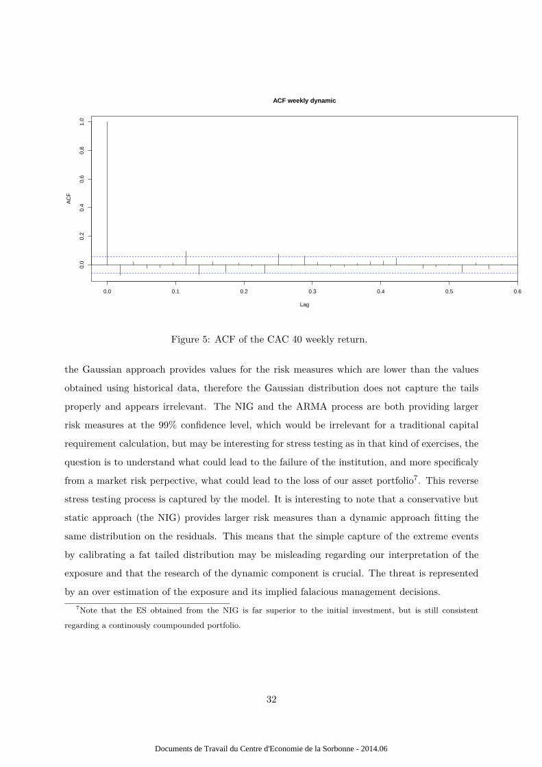
The p-value lower than 5% allows not to reject the stationarity assumption. Considering the

ACF and the PACF of the time series, respectivelly exhibited in figures 5 and 6, an ARMA(1,1)

has been adjusted on the data. Figure 6 exhibits some autocorrelations up to 22 weeks before the

latest. This could be consistent with the presence of long memory in the process. Unfortunately,

the estimation procedure failed estimating the parameters properly for both the ARFIMA and

the Gegenbaueur alternatives.

A NIG is fitted on the residuals. Parameters for the ARMA are presented in Table 4.1.2 and for

the NIG residuals distribution in Table 7.

ARMA φ1 = −0.3314, θ1 = 0.2593

Table 8 presents risk measures computed for each of the four approach implemented. In our case

31


0.0 0.1 0.2 0.3 0.4 0.5 0.6

0.0

0.2

0.4

0.6

0.8

1.0

Lag

AC

F

ACF weekly dynamic

Figure 5: ACF of the CAC 40 weekly return.

the Gaussian approach provides values for the risk measures which are lower than the values

obtained using historical data, therefore the Gaussian distribution does not capture the tails

properly and appears irrelevant. The NIG and the ARMA process are both providing larger

risk measures at the 99% confidence level, which would be irrelevant for a traditional capital

requirement calculation, but may be interesting for stress testing as in that kind of exercises, the

question is to understand what could lead to the failure of the institution, and more specificaly

from a market risk perpective, what could lead to the loss of our asset portfolio7. This reverse

stress testing process is captured by the model. It is interesting to note that a conservative but

static approach (the NIG) provides larger risk measures than a dynamic approach fitting the

same distribution on the residuals. This means that the simple capture of the extreme events

by calibrating a fat tailed distribution may be misleading regarding our interpretation of the

exposure and that the research of the dynamic component is crucial. The threat is represented

by an over estimation of the exposure and its implied falacious management decisions.

7Note that the ES obtained from the NIG is far superior to the initial investment, but is still consistent

regarding a continously coumpounded portfolio.

32


α µ σ γ

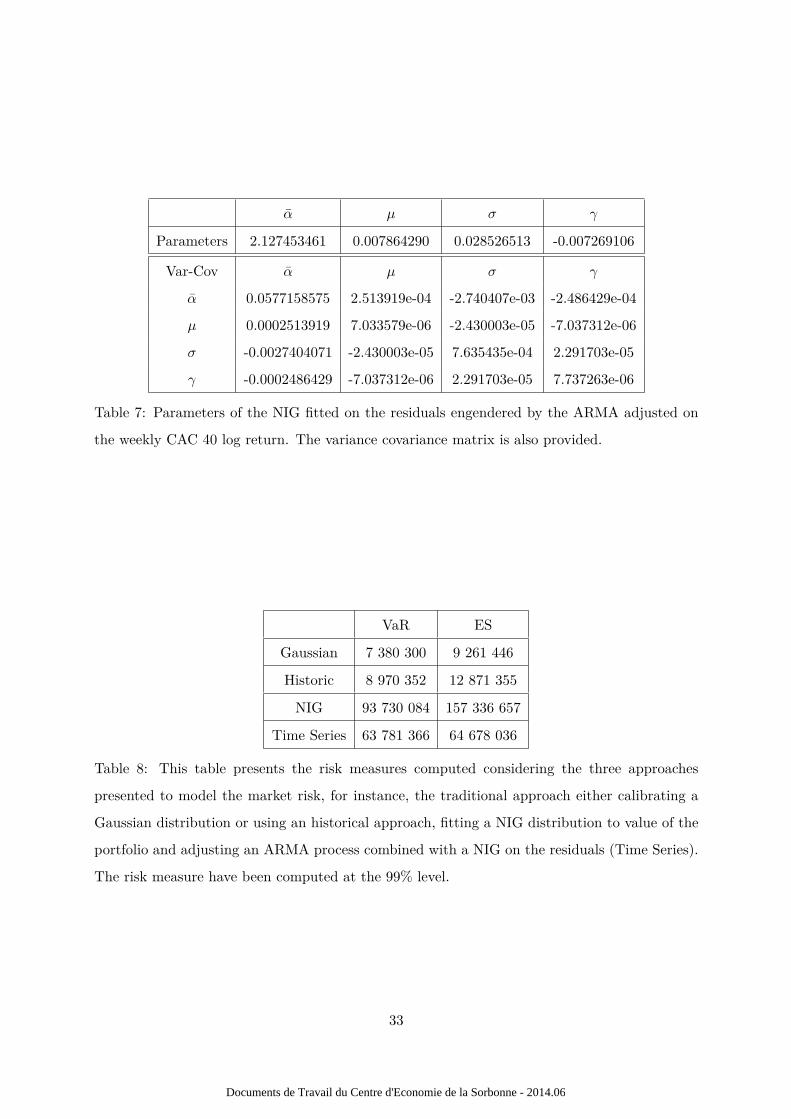
Parameters 2.127453461 0.007864290 0.028526513 -0.007269106

Var-Cov α µ σ γ

α 0.0577158575 2.513919e-04 -2.740407e-03 -2.486429e-04

µ 0.0002513919 7.033579e-06 -2.430003e-05 -7.037312e-06

σ -0.0027404071 -2.430003e-05 7.635435e-04 2.291703e-05

γ -0.0002486429 -7.037312e-06 2.291703e-05 7.737263e-06

Table 7: Parameters of the NIG fitted on the residuals engendered by the ARMA adjusted on

the weekly CAC 40 log return. The variance covariance matrix is also provided.

VaR ES

Gaussian 7 380 300 9 261 446

Historic 8 970 352 12 871 355

NIG 93 730 084 157 336 657

Time Series 63 781 366 64 678 036

Table 8: This table presents the risk measures computed considering the three approaches

presented to model the market risk, for instance, the traditional approach either calibrating a

Gaussian distribution or using an historical approach, fitting a NIG distribution to value of the

portfolio and adjusting an ARMA process combined with a NIG on the residuals (Time Series).

The risk measure have been computed at the 99% level.

33


0.0 0.1 0.2 0.3 0.4 0.5

−0.

050.

000.

050.

10

Lag

Par

tial A

CF

PACF weekly dynamic

Figure 6: PACF of the CAC 40 weekly return.

4.1.3 Operational Risks

This section describes how risks are measured considering three different approaches: the first

one corresponds to the traditional Loss Distribution Approach (Guégan and Hassani (2009),

Hassani and Renaudin (2013), Guégan and Hassani (2012b)), the second assumes that the losses

are strong white noises (they evolve in time but independently)8, and the third one filters the

data sets using the time series processes developed in the previous sections. In the next para-

graphs, the methodologies are detailed in order to associate to each of them the corresponding

capital requirement through a specific risk measure. According to the regulation, the capital

charge should be a Value-at-Risk (VaR) (Riskmetrics (1993)), i.e. the 99.9th percentile of the

distributions obtained from the previous approaches. In order to be more conservative, and to

anticipate the necessity of taking into account the diversification benefit (Guégan and Hassani

(2013a)) to evaluate the global capital charge the expected shortfall (ES) (Artzner et al. (1999))

has also been evaluated. The ES represents the mean of the losses above the VaR therefore this

risk measure is informed by the tails of the distributions.

8This section presents the methodologies applied to weekly time series, as presented in the result section. They

have also been applied to monthly time series.

34


Traditional Scheme To build the traditional loss distribution function we proceed as follows.

Let p(k, λ) be the frequency distribution associated to each data set, F (x; θ), the severity distri-

bution, then the loss distribution function is given by G(x) =∑∞

k=1 p(k; λ)F ⊗k(x; θ), x > 0, with

G(x) = 0, x = 0. The notation ⊗ denotes the convolution (?) operator between distribution

functions and therefore F ⊗n the n-fold convolution of F with itself. Our objective is to obtain

annually aggregated losses by randomly generating the losses. A distribution selected among the

Gaussian, the lognormal, the logistic, the GEV (Guégan and Hassani (2012a)) and the Weibull

is fitted on the severities. A Poisson distribution is used to model the frequencies. As losses are

assumed i.i.d., the parameters are estimated by MLE9.

Capturing the Fat Tails The operational risk approach is similar to the one presented in

the previous paragraph. A lognormal distribution is used to model the body of the distribution

while a GPD is used to characterise the right tail (Guégan et al. (2011)). A conditional Maxi-

mum likelihood is used to estimate the parameters of the body while a traditional MLE is used

for the GPD on the tail.

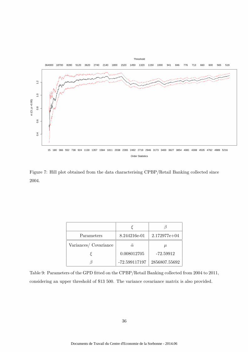
Using the Hill plot (Figure 7), the threshold has been set at $13 500. This means that 99.3%

of the data are located below. However, 407 data points remains above this threshold. The

parameters estimated for the GPD are given in table 9 along their variance-covariance matrix.

The parameters obtained fitting the lognormal distribution on the body of the distribution, i.e.

on the data below the threshold, are given in table 10 along their hessian. The VaR obtained

with this approach equals $31 438 810 and the Expected Shortfall equals $ 97 112 315.

Capturing the dynamics For the second approach (Guégan and Hassani (2013b)), in a first

step, the aggregation of the observed losses provides the time series (Xt)t. These weekly losses

are assumed to be i.i.d. and the following distributions have been fitted on the severities: the

Gaussian, the lognormal, the logistic, the GEV and the Weibull distributions. Their param-

eters have been estimated by MLE. Then 52 data points have been generated accordingly by

9Maximum Likelihood Estimation

35


15 180 366 552 738 924 1130 1357 1584 1811 2038 2265 2492 2719 2946 3173 3400 3627 3854 4081 4308 4535 4762 4989 5216

0.4

0.6

0.8

1.0

1.2

364000 18700 8280 5120 3620 2740 2140 1800 1520 1450 1320 1150 1000 941 846 776 713 660 600 565 519

Order Statistics

xi (

CI,

p =

0.95

)

Threshold

Figure 7: Hill plot obtained from the data characterising CPBP/Retail Banking collected since

2004.

ξ β

Parameters 8.244216e-01 2.172977e+04

Variances/ Covariance α µ

ξ 0.008012705 -72.59912

β -72.599117197 2856807.55692

Table 9: Parameters of the GPD fitted on the CPBP/Retail Banking collected from 2004 to 2011,

considering an upper threshold of $13 500. The variance covariance matrix is also provided.

36


µ σ

Parameters 4.068128 1.917474

hessian µ σ

µ 10318.2793 -678.7544

σ -678.7544 19134.8783

Table 10: Parameters of the Lognormal distribution fitted on the CPBP/Retail Banking collected

from 2004 to 2011, considering an upper threshold of $13 500. The hessian is also provided.

Monte Carlo simulations and aggregated to create an annual loss. This procedure is repeated

a million times to create a new loss distribution function. Contrary to the next approach, the

losses are aggregated over a period of time (for instance, a week or a month), but no time se-

ries process is adjusted on them, and therefore no autocorrelation phenomenon is being captured.

With the third approach the weekly data sets are modelled using an AR, an ARFI and a Gegen-

bauer process when it is possible. Table 11 provides the estimates of the parameters for the time

series processes. For The residuals a distribution is selected among the Gaussian, the lognormal,

the logistic, the GEV and the Weibull distributions. Their parameters are provided in Table

12. To obtain annual losses, 52 points are randomly generated from the residuals’ distributions

(εt)t from which the sample mean have been subtracted, proceeding as follows: if ε0 = X0

corresponds to the initialisation of the process, X1 is obtained applying one of the appropriate

adjusted stochastic processes to X0 and ε1, and so on, and so forth until X52. The 52 weeks

of losses are aggregated to provide the annual loss. Repeating this procedure a million times

enables creating another loss distribution function.

The first remark is that, focusing on the distributions selected before, the adequacy tests may

be misleading as the values are not conservative at all. The distributions have been adjusted on

the residuals arising from the adjustment of the AR, the ARFI and the Gegenbauer processes.

However, to conserve the white noise properties, the mean of the samples has been subtracted

from the generated value, therefore, the distribution which should be the best according to the

Kolmogorov-Smirnov test may not be in reality the most appropriate. As highlighted in Table

37


Weekly Aggregated loss time series on the cell (Client, Product and Business Practices / Retail Banking)

Time

Loss

Mag

nitu

des

2004 2005 2006 2007 2008 2009 2010 2011

050

0000

1000

000

1500

000

2000

000

2500

000

Figure 8: The figure represents the weekly aggregated loss time series on the cell CPBP/Retail

Banking collected since 2004.

13, the use of two sided distributions lead to lower risk measures while one sided distributions

lead to more conservative risk measures. Besides, these are closer to those obtained from the

traditional LDA meanwhile the autocorrelation embedded within the data has been captured.

It is also interesting to note that there is not an approach always more or less conservative than

the others. The capital charge depends on the strategy adopted and the couple selected: time

series process and residuals distribution. For instance a Gegenbauer process associated to a

lognormal distribution on CPBP / RB will be slightly more conservative than the traditional

approach and enables the capture time dependency, long memory, embedded seasonality and

larger tail. As a result, this may be a viable alternative approach to model the risks. The

distribution generating the white noise has a tremendous impact on the risk measures. From

Table 13, we observe that even if the residuals have an infinite two-sided support, they have some

larger tails and an emphasised skewness. Therefore, even if the residuals have been generated

using one sided distribution, as the mean of the sample has been subtracted from the values

to ensure they remain white noises, the pertaining distributions have only been shifted from a

38


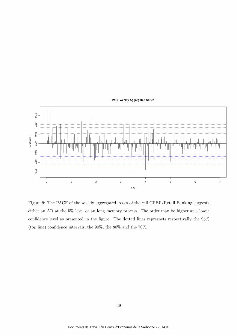
0 1 2 3 4 5 6 7

−0.

15−

0.10

−0.

050.

000.

050.

100.

15

Lag

Par

tial A

CF

PACF weekly Aggregated Series

Figure 9: The PACF of the weekly aggregated losses of the cell CPBP/Retail Banking suggests

either an AR at the 5% level or an long memory process. The order may be higher at a lower

confidence level as presented in the figure. The dotted lines represnets respectivally the 95%

(top line) confidence intervals, the 90%, the 80% and the 70%.

39


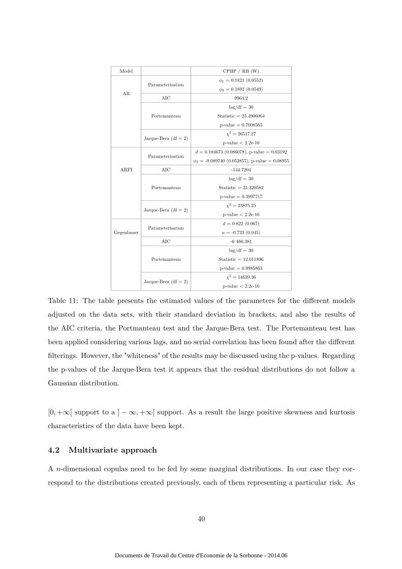
Model CPBP / RB (W)

AR

Parameterisationφ1 = 0.1821 (0.0552)

φ9 = 0.1892 (0.0549)

AIC 9964.2

Portemanteau

lag/df = 30

Statistic = 25.4906064

p-value = 0.7008565

Jarque-Bera (df = 2)χ2 = 26517.27

p-value < 2.2e-16

ARFI

Parameterisationd = 0.184673 (0.086078), p-value = 0.03192

φ2 = -0.089740 (0.052857), p-value = 0.08955

AIC -144.7204

Portemanteau

lag/df = 30


p-value = 0.3997717

Jarque-Bera (df = 2)χ2 = 23875.25

p-value < 2.2e-16

GegenbauerParameterisation

d = 0.822 (0.067)

u = -0.723 (0.045)

AIC -6 466.381

Portemanteau

lag/df = 30


p-value = 0.9985863

Jarque-Bera (df = 2)χ2 = 14639.36

p-value < 2.2e-16

Table 11: The table presents the estimated values of the parameters for the different models

adjusted on the data sets, with their standard deviation in brackets, and also the results of

the AIC criteria, the Portmanteau test and the Jarque-Bera test. The Portemanteau test has

been applied considering various lags, and no serial correlation has been found after the different

filterings. However, the "whiteness" of the results may be discussed using the p-values. Regarding

the p-values of the Jarque-Bera test it appears that the residual distributions do not follow a

Gaussian distribution.

[0, +∞[ support to a ] − ∞, +∞[ support. As a result the large positive skewness and kurtosis

characteristics of the data have been kept.

4.2 Multivariate approach

A n-dimensional copulas need to be fed by some marginal distributions. In our case they cor-

respond to the distributions created previously, each of them representing a particular risk. As

40


exhibited in Guégan and Hassani (2013a), the choice of the model to characterise a certain risk

plays an important role in the measurement of the exposure whatever the method used for the

dependence structure. In the previous section, various methodologies are introduced to fit the

appropriate dependence structure, for instance the nested strategies (Partially, Fully and Hier-

archical) or the pair-copula decomposition such as the D-Vine and the R-Vine (Joe (1997b)).

While for the nested structure the dependence intensity has to decrease as the level of nesting

increases the limitation of the vines is found in the number of decompositions we have to con-

sider as the number of vines grows exponentially with the dimension of the data set and thus

requires the user to select a vine from n!2 possible vines. For optimal selection strategies, we

refer the interested reader to Capéraà et al. (2000), Galambos (1978), Brechmann et al. (2010)

and Guégan and Maugis (2011).

In our case, the number of marginal distributions are limited as we only considered the three

main risks therefore the calibration strategies introduced earlier may not be necessary and a sim-

ple maximum likelihood estimation associated to the appropriate optimization algorithm may

be sufficient. However, as soon as another marginal distribution is considered, these have to be

implemented to ensure a proper parametrization of the dependence structure.

A crisis is characterized by asymmetric shocks translated into upper tail dependencies. Tra-

ditional approaches use either linear correlation in the sense of Pearson (Pearson (1900)), or

Gaussian copulas. In the best case scenarios, Student copulas are also used. Unfortunately this

latter copula with 3 degrees of freedom is symmetrical therefore the partially captured upper

tail dependence is naturally translated in a modeled lower tail dependence even if small losses

are independent. Besides, these structure are far from being conservative enough. Our stress-

testing objective imposes other copulas like for instance the Archimedean or Extreme value

copulas characterized by upper tail dependences such as the Gumbel copula, the Galambos cop-

ula (Koehler and Symanowski (1995)), the Husler-Reiss (Caputo (1998)) or the Tawn copula

(Silverman (1986)). Figure 10 compare the dependence structure obtained from a Gaussian

copula (ρ = 0.5) to the one obtained from a Gumbel (φ = 5). The concentration of dots in the

top right hand corner of the figure is characteristic of an upper tail dependence.

41


●

●

●

●

●

●

●

●

●

●

●

●

●●

●

●

●

●

●

●●

●

●

●●

●

●

●

●

●

●

●

●

●

●

●

●

●

●

●

●

●

●

●

●

●

●

●

●

●

●●

●

●

●

●

●

●

●

●

●

●

●

●

●

●

●

●

●

●

●

●

●●

●

●

●

●

●

●

●

●

●

●

●

●

●

●

●

●

●

●

●

●

●

●

●

●

●

●

●

●

●

●

●

●

●

●

●

●

●

●

●

●

●

●

●

●

●

●

●

●

●

●

●

●

●

●●

●

●

●

●

●

●

●

●

●

●

●

●

●

●

●

●

●

●

●

●

●

●

●

●

●

●

●

●

●

●

●●

●

●

●

●

●

●

●

●

●

●

●

●

●

●

●

●

●

●

●

●

●

●

●

●

●

●

●

●

●

●

●

●●

●

●

●

●

●

●

●

●

●

●

●

●●

●

●

●

●

●

●

●

●

●

●

●●

●

●

●

●

●

●

●

●

●

●

●

●

●

●

●

●

●

●

●

●

●

●

●

●

●

●●

●

●

●

●

●

●

●

●

●

●

●

●

●

●

●

●

●

●

●

●●

●

●

●

●

●

●

●

●

●

●

●

●

●

●

●

●

●

●

●

●

●

●

●

●

●

●

●

●

●

●

●

●

●

●

●

●

●

●

●

●

●

●

●

●

●

●

●

●

●

●

●

●

●

●

●

●

●

●

●

●

●

●

●

●

●

●

●

●

●

●

●

●

●

●

●

●

●

●

●

●

●

●

●

●

●

●

●

●

●●

●

●

●

●

●

●

●

●

●

●

●

●

●

●

●

●●

●

●

●

●

●

●

●

●

●

●

●

●●

●

●

●

●

●

●

●

●

●

●

●

●

●

●

●

●

●

●

●

●

●

●

●

●

●

●

●

●

●

●

●

●

●

●

●

●

●

●

●

●

●

●

●

●

●

●

●

●

●●

●

●

●

●

●

●

●

●

●

●●

●●

●

●

●

●

●

●

●

●

●

●●

●

●

●

●

●

●

●

●

●

●

●

●

●

●

●

●

●

●

●

●

●

●

●●

●

●

●

●

●

●

●

●●

●

●

●

●

●

●

●

●

●

●

●

●

●

●

●

●

●

●

●

●

●

●

●

●

●

●

●

●

●

●

●

●

●

●

●

●

●

●

●

●

●

●

●

●

●

●

●

●

●

●

●

●

●

● ●

● ●

●

●

●

●

●

●

●

●

●

●

●

●

●

●

●● ●

●

●

●

●

●

●

●

●

●

●

●

●

●

●

●

●

●

●

●●

●

●

●

●●

●

●

●

●

●

●

●

●

●

●

●

●

●

●

●

●

●

●

●

●

●

●

●

●

●● ●

●●

●

●

●

●

●

●

●

●

●

●

●

●

●

●

●

●

●

●

●

●

●

●

●

●

●

●

●

●

●

●

●

●

●

●

●

●

●

●

●

●●

●

●

●

●

●

●

●

●

●

●

●

●●

●

●

●

●

●

●

●

●

●

●

●

●

●●

●

● ●

●

●

●

●

●

●

●

●

●

●

●

●

●

●

●

●

●

●

●

●●

●

●

●

●

●

●

●

●

●

●

●

●

●

●

●

●

●

●

●

●

●

●

●

●

●

●

●

●

●

●

●

●

●

●

●

●

●

●

●

●

●

●

●

●

●

●

●

●

●

●

●

●

●

●

●

●

●

●

●

●

●

●

●

●

●

●

●

●

●

●

●

●

●

●

●

●

●

●

●

● ●

●

●

●

●

●

●

●

●

●

●

●

●

●

●

●

●

●

●

●

●

●

●

●

●

●

●

●

●

●

●

●

●

●

●

●

●

●

●

●

●

●

●

●

●

●

●

●

●

●

●

●

●●

●

●●

●

●

●

●

●

●

●

●

●

●

●

●

●

●

●

●

●

●

●

●

●

●

●

●

●

●

●

●

●

●

●

●

●

●

●

●

●

●

●●

●

● ●

●●

●●

●

●

●

●

●

●

●

●

●

●●

●

● ●

●

●

●

●●

●

●

●

●

●

●

●

●

●

●

●

●

●

●

●

●

●

●

●

●

●

●

●

●

●

●

●

●

●

●

●

●

●

●●

●

●

●

●

●

●

●

●

●

●

●

●

●

●

●

●

●

●

●

●

●

●

●

●

●

●

●

●

●

●

●

●

●

●

●

●

●

●

●

●

●

●

●

●

●

●

●

●

●

●

●

●

●

●

●

●

●

●

●

●●

●

●

●

●

●

●

●

●

●

●

●

●

●

●

●

●

●

●

●

●

●

●

●

●

●●

●

●

●

●

●

●

●

●

●●

●

●

●

●

●

●

●

●

●

●

●

●

●

●

●

●●

●

●

●

●

●

●

●

●

●

●

●

●

●

●

●

●

●

●

●

●

●

●

●

●

●

●

●

●

●

●

●

●

●

●

●

●

●

●

●

●

●

●

●●

●

●

●

●

●

●

●

●

●

●

●

●

●

●

●

●

●

●●

●

●

●

●

●

●

●

●

●

●

●

●

●

●

●

●

●

●

●

●

●

●

●

●

●

●

●

●

●

●

●

●●

●

● ●

●

●

●

●

●

●

●

●

●

●

●

●

●

●

●

●

●

●

●

●

●

●

●

●

●

●

●

●

●

●

●

●

●

●

●

●

●

●

●

●

●

●

●●

●

●

●

●

●

●

●

●

●

●

●

●

●

●

●

●

●

●

●

●

●

●

●

●

●

●

●

●

●

●

●

●

●

●

●

●

●

●

●

●

●

●

●

●

●

●

●

●

●

●

●

●

●

●

●

●

●

●

●

●

●

●

●

●

●

●

●

●

●

●

●

●

●

●

●

●

●

●

●

●

●

●

●

●

●

●

●

●

●

●

●

●

●

●

●

●

●

●

●

●

●

●

●●

●

●

●

●

● ●

●

●

●

●

●

●

●

●

●

●

●

●

●

●

●

●

●

●

●

●

●

●

●

●

●

●

●

●

●

● ●

●

●

●

●●

●

●

●

●

●

●

●

●

●

●

●

●

●

●

●

●

●

●

●

●

●

●

●

●

●

●

●

●

●

●

●

●

●

●

●

●

●

●

●

●●

●

●

●

●

●

●

●

●

●

●

●

●

●

●

●

●

●

●

●

●

●

●●

●

●

●

●

●

●

●

●●

●

●

●●●

●

●

●

●

●●

●

●

●

●

●

●

●

●

●

●

●

●

●

●

●

●

●

●

●

●

●

●

●

●

●

●

●

●

●

●

●

●

●

●

●

●

●

●

●

●

●

●

●

●●

●●

●

●

●

●

●

●

●

●

●

●●

●

●

●

●

●

●

●

●

●

●

●

●

●

●

●

●

●

●

●

●

●

●●

●

●

●

●

●

●

●●

●

●

●

●

●

●

●

●

●

●

●

●

●

●

●

●

●

●

●

●

●

●

●

●

●

●

●

●

●●

●

●

●

●

●

●

●

●

●

●

●●

●

●

●

●

●

●

●

●

●

●

●

●

●●

●

●

●

●

●

●

●

●

●

●

●

●●

●

●

●

●

●

●

●

●

●

●

●

●

●

●

●

●

●

●

●

●

●●

●

●

●

●

●

●

●

●

●

●

●

●

●

●

●

●

●

●

●

●

●

●

●

●

●

●

●

●

●

●

●●

●

●

●

●

●

●

●

●

● ●

●

●

●

●

●

● ●● ●

●

●

●

●

●

●

●

●

●

●

●

●

●

●

●

●

●●

●

●

●●

●

●

●

●

●

●

●

●

●

●

●

●

●

●

●

●

●

●

●

●

●

●

●

●

●

●

●

●

●

●

●

●

●

●

●

●

●

●

●

●

●

●

●

●

●

●

●

●

●

●

●

●

●

●

●

●

●

●

●

●

●

●

●

●

●

●

●

●

●

●

●

●

●

●

●

●

●

●

●

●

●

●

●

●

●

●

●

●

●

●

●

●

●

●

●

●

●

●

●

●

●

●

●

●

●

●

●

●

●

●

●

●

●

●

●

●

●

●

●

●

●

●

●

●

●

●

●●

●

●

●

●

●

●

●

●

●

●

●

●

●

●

●

●

●

●

●●

●

●

●

●

●

●

●

●

●

●

●

●●

●

●

●

●

●

●

●

●

●●

●

●

●

●

●

●

●

●

●

●●

●

●

●

●

●

●

●

●

●

●

●

●

●

●

●

●

●

●

●

●

●

●

●

●

●

●

●

●

●

●

●

●

●

●

●

●

●

●

●

●

●

●

●

●●

●

●

●

●

●

●

●

●

●

●●

●

●

●

●

●

●

●

●

●

●

●

●

●

●

●

●

●

●

●

●

●●

●

●

●

●

●

●●

●

●

● ●

●

●

●

●

●

●

●

●●

●

●

●

●

●

●

●●

●

●

●

●

●

●

●

●

●

●

●

●

●

●

●

●

●

●

●

●

●

●

●

●

●

●

●

●

●

●

●

●

●

●

●

●

●

●

●

●

●

●

●

●

●

●

●

●

●

●

●

●

●

●

●

●

●

●

●

●

●

●

●

●

●

●

●

●

●

●

●

●

●

●

●

●

●

●

●

●

●

●

●

●

●

●

●

●

●

●

●

●

●

●

●

●

●

●

●

●

●

●

●

●

●

●

●

●●

●●

●●

●

●

●

●

●

●

●

● ●

●

●

●

●

●

●

●

●

●

●●

●

●

●

●

●

●

●

●

●

●

●

●

●

●

●

●

●

●

●

●

●

●

●

●

●

●

●●

●●

●

●

●

●

●

●

●

●●

●

●

●

●

●

●

●

●

●

●

●

●

●

●

●

●

●

●

●

●

●

●

●

●

●

●

●

●

●

●

●

●

●

●

●

●

●

●

●

●

●

●

●

●

●

●

●

●

●

●

●

●

●

●

●

●

●

●

●

●

●

●

●

●

●

●

●

●

●

●

●

●

●

●

●

●

●

●

●

●

●

●

●

●

●

●

●

●

●

●

●

●

●

●

●

●

●

●

●

●

●

●

●

●

● ●

●

●

●

●

●

●

●

●

●

●

●●

●

●

●

●

●

●

●

●

●

●

●

●

●

●

●

●

●

●

●

●

●

●

●

●

●

●●

●

●

●

●

●

●

●●

●

●

●

●

●

●

●

●

●

●

●

●

●

●

●

●

●

●

●

●

●

●

●

●

●

●

●

●

●

●

●

●

●

●

●

●

●

●

●

●

●

●

●

●

●

●

●

●

●

●

●

●

●●

●

●

●

●

●

●

●

●

●

●

●

●

●

●

●

●

●

●

●

●

●

●

●

●

●

● ●●

●

●●

●

●

●

●

●

●

●

●

●

●

●

●

●

●

●

●

●

●

●

●

●

●

●

●

●

●

●

●

●

●

●

●

●

●

●

●

●

●

●

●

●

●

●

●

●

●

●

●

●

●

●

●

●

●

●

●

●

●

●

●

● ●

●

●●

●

●

●

●

●

●

●

●

●

●

●

●

●

●

●

●

●

●

●

●

●

●●

●

●

●

●

●●

●

●

●

●

●

●

●

●

●

●

● ●

●

●

●

●

0.0 0.2 0.4 0.6 0.8 1.0

0.0

0.2

0.4

0.6

0.8

1.0

Gaussian

●

●

●

●●

●

●

●

●

●

●

●

●

●

●

●

●

●

●

●

●

●

●

●

●

●

●

●

●

●

●

●

●

●

●

●

● ●

●

●

●

●

●

●

●●

●

●

● ●

●

●

●

●

●

●

●

●

●

●

●

●

●

●

●

●

●

●

●

●

●

●

●

●

●

●

●

●

●

●

●

●

●●

●

●

●

●

●

●

●

●

●

●

●

●

●

●

●●

●

●

●

●

●

●

●

●

●

●

●

●

●

●

●

●

●

●

●

●

●

●

●

●

●

●

●

●

●

●

●

●

●

●

●

●

●

●

●

●

●

●

●

●

●

●

●

●

●

●

●

●●

●

●

●

●

●

●

●

●

●

●

●

●

●

●

●

●

●

●●

●

●

●

●

●

●

●

●

●●

●

●

●

●

●

●

●

●

●

●

●

●

●

●

●

●

●

●

●

●

●

●

●●

●

●

●

●

●

●

●

●

●

●

●

●

●

●

●

●

●

●

●

●

●

●●

●

●

●

●

●

●

●

●

●

●

●

●

●

●

●

●

●

●

●

●

●

●

●

●

●

●

●

●

●

●

●

●

●

●

●

●

●

●

●

●

●

●

●

●

●

●

●

●

●

●

●

●

●

●

●

●

●

●

●

●

●

●

●

● ●

●

●

●

●

●

●

●

●

● ●

●

●

●

●

●

●

●

●

●

●

●

●

●

●

●

●

●●

●

●

●

●

●

●

●

●

●

●

●

●

●

●

●

●

●

●

●

●

●

●

●

●

●

●

●

●

●

●

●

●

●

●●

●

●

●

●

●

●

●

●

●

●

●

●

●

●

●

●

●

●

●

● ●

●

●

●●

●●

●

●

●

●

●

●

●

●

●

●

●

●

●

●

●

●

●

●

●

●

●

●

●

●

●

●

●

●●

●

●

●

●

●

●

●

●

● ●

●

●

●

●

●

●

●

●

●

●

●●

●●

●

●

●

●

●

●●

●

●

●

●

●

●

●

●

●

●

●

●

●

●

●

●

●

●

●

●

●

●

●

●

●

●

●

●

●

●

●

●

●

●

●

●

●

●

●

●

●

●

●

●

●

●

●

●

●

●

●

●

●

●

●

●

●

●

●

●

●

●

●

●

●

●

●

●

●

●

●

●

●

●

●

●

●

●

●

●

●

●●

●

●

●●

●

●

●

●

●

●

●

●

●

●

●

●

●

●

●

●

●

●

●

●

●

●

●

●

●

●

●

●●

●

●

●

●

●

●

●

●

●

●

●

●

●●

●

●

●

●

●

●

●

●

●

●

●

●

●

●

●

●

●

●

●

● ●

●

● ●

●

●

●

●

●

●

●

●

●

●

●

●

●

●

●

●

●

●

●

●●

●

●

●

●

●

●

●

●

●

●

●

●

●

●

●

●

●

●

●

●

●

●

●

●

●

●

●

●

●●

●

●

●

●

●●

●

●

●

●

●

●

●

●

●●

●

●●

●●

●

●

●

●

●

●

●

●

●

●

●

●

●

●

● ●

●

●

●

●

● ●

●

●

●

●

●

●

●

● ●

●

●

●

●

●

●

●

●

●

●

●

●

●

●●

●

●

●

●

●

●

●

●

●

●

●

●

●

●

●

●

●

●

●

●

●

●

●

●

●

●

●

●

●

●

●

●

●

●

●

●

●

●

●

●

●

●

●

●

●

●

●

●

●

●

●

●

●

●

●

●

●

●

●

●

●

●

●

●

●

●

●

●

●

●

●

●

●●

●

●

●

●

●

●

●

●

●

●

●

●

●

●

●

●

●

●

●

●

●

●

●

●●

●

●

●

●

●

●

●

● ●

●

●

●

●

●

●

●

●●

●

●

●

●

●

●

●

●

●

●

●

●

●

●

●

●

●

●

●

●

●

●●

●

●

●

●

●

●

●

●

●

●

●

●

●

●

●

●

●

●

●

●

●

●

●

●

●

●

●

●

●

●

●

●

●

●

●

●

●

●

●●

●

●

●

●

●

●

●

●

●

●

●

●

●

●

●

●

●

●

●

●

●

●

●

●●●

●

●

●

●

●

●

●

●

●

●

●

●

●

●

●

●

●

●

●

●

●

●

●

●

●

●

●

●

●

●

● ●

●

●

●

●

●

●

●

●

●

●

●

●

●

●

●

●

●

●

●●

●

●

●

●

●

●

●

●

●

●

●

●

●

●

●

●

●

●

●●

●

●

●

●

●

●

●

●

●

●

●

●

●

●

●

●

●

●

●

●

●

●

●

●

●

●

●

●

●

●

●

●

●

●

●

●

●

● ●

●

●

●

●

●

●

●

●

●●

●

●

●

●

●

●

●

●

●

●

●

●

●

●

●

● ●

●

●

●

●

●

●

●

●

●

●

●

●

●

●

●

●

●

●

●

●●

●●

●

●

●

●

●

●

●●

●

● ●

●

●

●

●

●

●●

●

●

●●

●

●

●●

●

●

●

●

●

●

●

●

●

●

●

●

●

●

●

●

●

●●

●

●

●

●

●

●

●

●

●

●

●

●

●

●

●

●

●

●

●

●

●

●

●

●

●●

●

●

●

●

●

●

●

●

●

●

●

●

●

●

●

●

●

●

●

●

●

●

●

●●

●

●

●

●

●

●

●

●

●

●

●

●

●

●

●

●

●

●

●

●

●

●

●

●

●

●

●

●

●

●

●

●

●

●

●

●

●

●

●

●

●

●●

●

●

●

●

●

●

●

●

●

●

●

●

●

●

●

●

●

●

●

●

●

●

●

●

●

●

●

●

●

● ●

●

●●

●

●

●

●

●

●

●

●

●

●

●

●

●

●

●

●

●

●

●

●

●

●

●

●

●

●

●

●

●

●

● ●

●

●

●

●

●

●

●●

●

●

●

●

●

●

●

●

●

●

●

●

●

●

●

●

●

●

●

●

●

●

●

●

●

●

●

●

●

●

●

●

●

●●

●

●

●

●

●

●

●

●

●

●●

●

●

●●

●

●

●

●

●

●

●

●

●

●

●

●

●

●

●

●

●

●

●

●

●

●

●

●

●

●

●

●

●

●

●

●

●

●

●

●

●●

●●

●

●

●

●

●

●

●

●

●

●

●

●

●●

●

●

●

●

●

●

●

●

●

●

●

●

●

●

●

●

●

●

●

●

● ●

●

●

●

●

●

●

●

●

●

●

●

●

●

●

●

●

●

●

●

●

●

●

●

● ●

●

●

●

●

●

●

●

●

●

●

●

●

●

●

●

●

●

●

●

●

●

●

●

●

●

●

●

●

●

●

●

●

●

●

●

●

●

●

●

●

●

●

●

●

●

●

●

●

●

●

●

●

●

●

●

●

● ●

●

●

●

●

●

●●

●

●

●

●

●

●

●

●

●

●

●

●

●

●

●

●

●

●

●

●

●

●

●

●

●

●

●

●

●

●

●

●●

●

●

●

●

●

●

●

●

●

●

●

●

●

●

●

●

●

●

●

●

●

●

●

●

●

●●

●

●

●

●

●

●

●

●

●

●

●

●

●●

●

●

●

●

●

●

●

●

●

●

●

●

●

●●

●

●

●

●

●

●

●

●

●

● ●

●

●

●

●

●

●

●

●

●

●

●

●

●

●

●

●

●

●

●

●

●

●

●

●

●

●

●●

●

●●

●

●

●

●

●

●

●

●

●

●

●

●

●

●

●

●

●

●

●

●

●●

●

●

●

●

●

●

●

●

●

●

●

●

●

●●

●

●●

●

●

●

●

●

●

●

●

● ●

●

●

●

●

●

●

●

●

●

●

●

●

●

●

●

●

●

●

●

●

●

●

●

●

●

●

●

●●

●

●

●

●

●

●

●

●

●

●

●

●

●

●

●

●

●

●

●

●

●

●

●

●

●

●

●

●

●

●

●●

●

●

●

●

●

●

●

●

●

●

●

●

●●

●

●

●

●

●

●

●

●

●

●

●

●

●

●

●

●

●

●

●

●●

●●

●●

●

●

●

●

●

●

●

●

●

●

●

●

●

●

●

●

●

●

●

●

●

●

●

●

●

●

●

●

●

●

●

●

●

●

●

●

●

●

●

●

●

●●

●

●

●●

●

● ●●

●

●

●

●

●

●

●

●

●●

●

●●

●

●

●

●

●

●

●

●

●

●

●

●

●

●

●

●

●

●

●

●

●

●

●

●

●

●

●

●

●

●

●

●

●

●

●

●

●●

●

●

●

●

●

●

●

●●

●

●

●

●

●

●

●

●

●

●

●

●●

●

●

● ●

●

●

●

●

●

●

●

●

●

●

●

●

●

●

●

●

●

●

●

●

●

●

●

●

●

●●

●

●

●

●

●

●

●

●

●

●

●

●

●

●

●

●

●

●

●

●

●

●

●

●

●

●

●

●

●

●

●

●

●

●

●

●

●

●

●

●

●

●

●

●

●

●

●

●

●●

●

●

●

●

●

●

●

●

●

●

●

●

●

●

●

●

●

●

●

●

●

●

●

●

●●

●

●

●

●

●

●

●

●

●

●

●

●●

●

●

●

●

●

●

●

●

●

●

●

●

●

●

●

●

●

●

●

●

●

●

●

●

●

●

●

●

●

●

●

●

●

●

●

●

●

●

●

●

●

●

●

●

●

●

●

●

●

●

●

●

●

●

●

●

●

●

●

●

●

●

●

●

●

●

●●

●

●

●

●

●

●

●

●

●

●

●

●

●

●

●

●

●

●●

●

●●

●

●

●

●

●

●

●

●

●

●

●

● ●

●

●

●

●

●

●

●

●

●

●

●

●

●

●

●

●

●

●

●

●

●

●

●

●

●

●

● ●

●

●

●

●

●

●

●

●

●

●

●

●

●

●

●

●

●

●

●

●

●

●

●

●

●

●

● ●

●

●

●

●

●

●

●

●

●

●

●

●

●

●

●

●

●

●

●

●

●

●

●

●

●

●

●

●

●

●

●

●

●

●

●

●

●

●

●

●

●

●

●● ●

●

●

●

●●

●

●

●

●

●

●

●

●

●

●

●

●

●

●

●

●

●

●

●

●

●

●

●

●

●

●

●

●

●

●

●

●

●

●

●

●

●

●

●

●

●

● ●

●

●

●

●

●

●

●

●

●

●

●

●

●

●

●

●

●

●

●

●

●

●

●

●

●

●

●

●

●

●

●

●

●

●

●

●

●

●

●

●

●

●

●

●

●

●

●

●

●

●

●

●

●

●

●

●

●

●

●

●●

●

●

●

●

●

●

●

●

●

●

●

●

●

●

●

●

●

●

●

●

●●

●

●

●

●●

●

●

●

●

●

●

●

●

●

●

●

●

●

●

●

●

●

●

●●

●

●

●

●

●

●

●

●

●

●

●

●

●

●

●

●

●

●

●

●

●

●

●

●

●

●

●

●

●

●

●

●

●

●

●

●

●●

●

●

●

●

●

●

●

●

●

●

●

●

●

●

●

●

●

●

●

●

●

●

●

●

●

●●

●

●

●

●

●

●

●

●

●

●

●

●

●

●

●

●

●

●

●

●

●

●

●

●

●

●

●

●

●

●

●

●

●

●

●

●

●

●

0.0 0.2 0.4 0.6 0.8 1.0

0.0

0.2

0.4

0.6

0.8

1.0

Gumbel

Figure 10: The figure compares the Gaussian copula with a parameter equals 0.5 and a Gum-

bel copula with a parameter equals to 5. The Gumbel copula shape exhibit some upper tail

dependency.

42


Applying these two last copulas to the various traditional marginal distributions constructed in

the previous subsections led us to the risk measures presented in the Table 14. We note that the

Gumbel copula provides a more conservative capital requirement illustrating the lower impact

of the diversification benefit. These results have been obtained for assets whose correlation is

not particularly high: ρCredit,Market = 0.5, ρCredit,Operational = 0.4, ρMarket,Operational = 0.4 for

the Gaussian copula, and φ1 = 5 for the Gumbel copula.

It is also interesting to note that the capture of an upper tail dependence behaviour implies the

capture of a contagion effect, which engenders larger losses during a turmoil than during a calm

business cycle.

43


References

Acerbi, C. and Tasche, D. (2002), ‘On the coherence of expected shortfall’, Journal of Banking

and Finance 26(7), 1487–1503.

Artzner, P., Delbaen, F., Eber, J.-M. and Heath, D. (1999), ‘Coherent measures of risk’, Math.

Finance 9 3, 203–228.

Barndorff-Nielsen, O. and Halgreen, C. (1977), ‘Infinite divisibility of the hyperbolic and

generalized inverse gaussian distributions’, Z. Wahrscheinlichkeitstheorie und Verw. Gebiete

38(4), 309–311.

BCBS (2006), ‘Basel committee: International convergence of capital measurement and capital

standards’, Bank for International Settlements, Basel .

Bedford, T. and Cooke, R. M. (2001), ‘Probability density decomposition for conditionally depen-

dent random variables modeled by vines.’, Annals of Mathematics and Artificial Intelligence

32, 245–268.

Beran, J. (1994), Statistics for Long-Memory Processes, CRC Press, New York.

Berg, D. and Aas, K. (2009), ‘Models for construction of multivariate dependence - a comparison

study’, The European Journal of Finance 15, 639–659.

Berkowitz, J. (1999), ‘A coherent framework for stress testing’, Federal Reserve Board, Wash-

ington, USA] .

Bollerslev, T. (1986), ‘Generalized autoregressive conditional heteroskedasticity’, Journal of

Econometrics 31(3), 307–327.

Brechmann, E., Czado, C. and Aas, K. (2010), ‘Truncated regular vines in high dimensions with

applications to financial data.’, Submitted preprint. .

Brockwell, P. and Davis, R. (1988), ‘Simple consistent estimation of the coefficients of a linear

filter’, Stoch. Proc. Appl. 28, 47–59.

Bunn, P., Cunningham, A. and Drehmann, M. (2005), ‘Stress testing as a tool for assessing

systemic risks’, Bank of England Stability Review June.

44


Capéraà, P., Fougères, A. and Genest, C. (2000), ‘Bivariate distributions with given extreme

value attractor.’, Journal of Multivariate Analysis 72, 30–49.

Caputo, A. (1998), ‘Some properties of the family of koehler-symanowski distributions.’, Working

Paper, The Collaborative Research Center (SBF), LMU-München .

Cleveland, W. (1979), ‘Robust locally weighted regression and smoothing scatterplots’, Journal

of the American Statistical Association 74(368), 829–836.

Delbaen, F. (2000), ‘Coherent risk measures’, Lecture Notes of the Cattedra Galileiana at the

Scuola Normale di Pisa .

Dissmann, J., Brechmann, E., Czado, C. and Kurowicka, D. (2011), ‘Selecting and estimating

regular vine copulae and application to financial returns.’, Submitted preprint. .

Engle, R. (1982), ‘Autoregressive conditional heteroscedasticity with estimates of the variance

of united kingdom inflation’, Econometrica 50(4), 987–1007.

Fayyad, U., Piatetsky-Shapiro, G. and Smyth, P. (1996), ‘From data mining to knowledge dis-

covery in databases’, AI Magazine 17(3), 37–54.

Galambos, J. (1978), The asymptotic theory of extreme order statistics., Wiley Series in Proba-

bility and Mathematical Statistics, JohnWiley & Sons, New York-Chichester-Brisbane.

Genest, C., Ghoudi, K. and Rivest, L.-P. (1995), ‘A semiparametric estimation procedure of

dependence parameters in multivariate families of distributions.’, Biometrika 82, 543–552.

Gourier, E., Farkas, W. and Abbate, D. (2009), ‘Operational risk quantification using extreme

value theory and copulas: from theory to practice.’, The Journal of Operational Risk 4.

Gregory, J. (2012), Counterparty Credit Risk and Credit Value Adjustment: A Continuing Chal-

lenge for Global Financial Markets, 2nd Edition edition, John Wiley & Sons, London.

Guégan, D. (2005), ‘How can we define the concept of long memory? an econometric survey’,

Econometric Review 24(2).

Guégan, D. and Hassani, B. (2012a), ‘A mathematical resurgence of risk management : an

extreme modeling of expert opinions.’, To appear in Frontier in Economics and Finance,

Documents de travail du Centre d’Economie de la Sorbonne 2011.57 - ISSN : 1955-611X .

45


Guégan, D. and Hassani, B. (2012b), ‘Operational risk: A basel ii++ step before basel iii.’,

Journal of Risk Management in Financial Institutions 6(1).

Guégan, D. and Hassani, B. (2013a), ‘Multivariate vars for operational risk capital computation

: a vine structure approach.’, International Journal of Risk Assessment and Management

(IJRAM) 17(2), 148–170.

Guégan, D. and Hassani, B. (2013b), ‘Using a time series approach to correct serial correlation

in operational risk capital calculation’, The Journal of Operational Risk 8(3), 31–56.

Guégan, D. and Hassani, B. K. (2009), ‘A modified panjer algorithm for operational risk capital

computation’, The Journal of Operational Risk 4, 53 – 72.

Guégan, D., Hassani, B. and Naud, C. (2011), ‘An efficient threshold choice for the computation

of operational risk capital.’, The Journal of Operational Risk 6(4), 3–19.

Guégan, D., Hassani, B. and Zhao, X. (2013), Emerging Countries Sovereign Rating Adjustment

using Market Information: Impact on Financial Institutions Investment Decisions, Academic

Press, Oxford.

Guégan, D. and Maugis, P.-A. (2010), ‘New prospects on vines.’, Insurance Markets and Com-

panies: Analyses and Actuarial Computations 1(1), 15–22.

Guégan, D. and Maugis, P.-A. (2011), ‘An econometric study for vine copulas.’, International

Journal of Economics and Finance 2(1), 2–14.

Hassani, B. K. and Renaudin, A. (2013), ‘The cascade bayesian approach for a controlled in-

tegration of internal data, external data and scenarios.’, Working Paper, Université Paris 1,

ISSN : 1955-611X [halshs-00795046 - version 1] .

Huggenberger, M. and Klett, T. (2009), ‘A g-and-h copula approach to risk measurement in

multivariate financial models’, Preprint, University of Mannheim, Germany .

Joe, H. (1997a), Multivariate models and dependence concepts., Monographs on Statistics and

Applied Probability, Chapman and Hall, London.

Joe, H. (1997b), Multivariate models and dependence concepts., Monographs on Statistics and

Applied Probability, Chapman and Hall, London.

46


Joe, H. (2005), ‘Asymptotic efficiency of the two-stage estimation method for copula-based

models.’, Journal of Multivariate Analysis 94, 401–419.

Koehler, K. and Symanowski, J. (1995), ‘Constructing multivariate distributions with specific

marginal distributions.’, J. Multivar. Distrib. 55, 261–282.

Leadbetter, M. (1983), ‘Extreme and local dependence in stationary sequences’, ZWVG 65, 291–

306.

Lorenz, E. N. (2010), ‘Deterministic nonperiodic flow’, Journal of the Atmospheric Sciences

20(2), 130–141.

Majnoni, G., Martinez-Peria, M. S., Blaschke, W. and Jones, M. T. (2001), ‘Stress testing of

financial systems: An overview of issues, methodologies and fsap experiences’, Working paper,

IMF .

McCulloch, J. (1996), ‘On the parametrization of the afocal stable distributions’, Bulletin of the

London Mathematical Society 28, 651–655.

Mendes, B., de Melo, E. and Nelsen, R. (2007), ‘Robust fits for copula models’, Comm. in Stat.:

Sim. Comp 36.

Merton, R. C. (1972), ‘On the pricing of corporate debt: The risk structure of interest rates’,

Journal of Finance 29, 449–470.

Morgan, J. (1997), ‘Introduction to creditmetrics’, Technical Document .

Pearson, K. (1900), ‘On the criterion that a given system of deviations from the probable in the

case of a correlated system of variables is such that it can be reasonably supposed to have

arisen from random sampling’, Philosophical Magazine Series 5 50(302), 157–175.

Pesola, J. (2007), ‘Financial fragility, macroeconomic shocks and banks’ loan losses: evidence

from europe’, Working Paper, Bank of Finland Research 15.

Quagliariello, M. (2009), Stress-testing the Banking System: Methodologies and Applications,

Cambridge University Press, London.

Riskmetrics (1993), ‘Var’, JP Morgan .

47


Rockafellar, R. and Uryasev, S. (2000), ‘Optimization of conditional value-at-risk’, Journal of

Risk 2(3), 21–41.

Rockafellar, R. and Uryasev, S. (2002), ‘Conditional value at risk for general loss distributions’,

Journal of Banking and Finance 26(7), 1443–1471.

Rodriguez, J.-C. (2007), ‘Measuring financial contagion: A copula approach’, Journal of Empir-

ical Finance 14, 401–423.

Said, S. and Dickey, D. (1984), ‘Testing for unit roots in autoregressive moving average models

of unknown order’, Biometrika 71, 599–607.

Sereda, E., Bronshtein, E., Rachev, S., Fabozzi, F., Sun, W. and Stoyanov, S. (2010), Distortion

Risk Measures in Portfolio Optimisation, Volume 3 of Business and Economics, Springer US.

Siddique, A. and Hasan, I. (2013), Stress Testing: Approaches, Methods and Applications, Risk

Books, London.

Silverman, B. W. (1986), Density Estimation for statistics and data analysis, Chapman and

Hall/CRC.

Sklar, A. (1959), ‘Fonctions de répartition à n dimensions et leurs marges’, Publ. Inst. Stat.

8, 229–231.

Taleb, N. (2010), The Black Swan: the impact of highly improbable, 2nd Edition, Random House

and Penguin, New York.

Taqqu, M. and Samorodnisky, G. (1994), Stable non-Gaussian random processes, Chapman and

Hall, New York.

Wang, S. S. (2000), ‘A class of distortion operators for pricing financial and insurance risks.’,

Journal of Risk and Insurance 67(1), 15–36.

Weiss, G. (2010), ‘Copula parameter estimation - numerical considerations and implications for

risk management’, Journal of Risk 13.

48


Distribution Traditional LDF Time Series LDF AR(9) ARFI(d,2) Gegenbauer

Severity GoF Severity GoF Residuals GoF Residuals GoF Residuals GoF

Gaussian µ = 775.60 , σ = 13449.39 < 2.2e − 16 µ = 125676.6 , σ = 240299.7 < 2.2e − 16 µ = −3.73e − 12, σ = 193951.9 2.716e − 13 µ = 213.66, σ = 210162.3 5.551e − 16 µ = −33271.55, σ = 187160.6 2.677e − 09

(55.77) , (1557.07) (12396.71) , (49772.55) (10321.18), (31866.62) (10549.58), (33898.01) (13697.62), (46220.53)

Lognormal µ = 4.12 , σ = 2.01 < 2.2e − 16 µ = 10.85 , σ = 1.55 0.0008751 µ = 10.86, σ = 1.39 < 2.2e − 16 µ = 10.90, σ = 1.45 < 2.2e − 16 µ = 10.28, σ = 1.43 < 2.2e − 16

(0.0147) , (0.00998) (0.081) , (0.092) (0.115), (0.0856) (0.118), (0.099) (0.171), (0.138)

Logistic µ = 146.16 , β = 702.67 < 2.2e − 16 µ = 117515.05 , β = 72633.31 < 2.2e − 16 µ = −14762.13, β = 52516.15 0.2351 µ = −22832.232, β = 51028.33 0.1166 µ = −11419.42, σ = 38697.341 0.1077

(4.199) , (2.813) (2097.15) , (2097.15) (2097.15), (1482.91) (2965.82), (2097.15) (2965.82), (1712.32)

GEV NA NA ξ = 7.37e − 01, β = 41154, 0.03361 NA NA ξ = −1.74e − 02, β = 173140, < 2.2e − 16 ξ = −2.04e − 01, β = 111700, 2.932e − 10

µ = 34506 µ = −87169 µ = −89320

NA (6.88e − 02) , (1537), (1387) NA (1.57e − 02), (1483), (2097) (2.003e − 06), (595.2), (2760)

Weibull ξ = 0.441 , β = 172.3 < 2.2e − 16 ξ = 0.62 , 51430 < 2.2e − 16 ξ = 0.752, β = 199529 < 2.2e − 16 ξ = 0.725, β = 210262 < 2.2e − 16 ξ = 0.662, β = 186161 < 2.2e − 16

(1.459e − 03), (2.096) (2.262e − 02) , (2326) (5.05e − 02), (4201) (4.94e − 02), (4199) (6.94e − 02), (5974)

Hyperbolic α = 569.74, µ − 9.37e − 04 < 2.2e − 16 NA NA α = 9.8845e − 06, δ = 1031.03, NA NA NA α = 1.33394e − 05, δ = 875.97, NA

δ = 3.40e − 06, β = 569.74 β = −3.088e − 11, µ = 6.003 β = −2.746983e − 06, µ = −1451.36

OD NA OD NA NA

Table 12: The table presents the parameters of the distributions fitted on either the i.i.d. losses or the residuals characterising the

CPBP / Retail Banking weekly aggregated. Traditional LDF denotes Frequency ⊗ Severity, Time Series LDF characterises the second

approach considering i.i.d. weekly losses, AR denotes the autoregressive process and both ARFI and Gegenbauer denote their related

processes. The standard deviations are provided in brackets. The Goodness-of-Fit (GoF) is considered to be satisfactory if the value

is > 5%. If it is not, then the distribution associated to the largest p-value is retained. The best fit per column are presented in bold

characters. Note: NA denotes a model "Not Applicable", and OD denotes results which may be provided "On Demand".

49

Docum

ents de Travail du C

entre d'Econom

ie de la Sorbonne - 2014.06

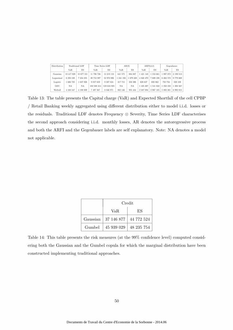
Distribution Traditional LDF Time Series LDF AR(9) ARFI(d,2) Gegenbauer

VaR ES VaR ES VaR ES VaR ES VaR ES

Gaussian 10 417 929 10 677 551 11 798 726 12 219 110 641 575 694 887 1 421 140 1 553 661 1 997 072 2 199 513

Lognormal 6 250 108 7 234 355 39 712 897 52 972 896 1 241 192 1 679 228 4 840 470 7 609 198 6 262 572 9 779 669

Logistic 1 606 725 1 637 926 9 057 659 9 307 824 317 715 350 396 628 637 692 862 750 756 830 100

GEV NA NA 182 588 314 519 616 925 NA NA 1 425 307 1 541 832 1 258 450 1 393 567

Weibull 4 168 547 4 198 009 7 497 567 8 046 971 882 146 955 434 2 587 094 2 967 185 5 892 381 6 992 815

Table 13: The table presents the Capital charge (VaR) and Expected Shortfall of the cell CPBP

/ Retail Banking weekly aggregated using different distribution either to model i.i.d. losses or

the residuals. Traditional LDF denotes Frequency ⊗ Severity, Time Series LDF characterises

the second approach considering i.i.d. monthly losses, AR denotes the autoregressive process

and both the ARFI and the Gegenbauer labels are self explanatory. Note: NA denotes a model

not applicable.

Credit

VaR ES

Gaussian 37 146 877 44 772 524

Gumbel 45 939 029 48 235 754

Table 14: This table presents the risk measures (at the 99% confidence level) computed consid-

ering both the Gaussian and the Gumbel copula for which the marginal distribution have been

constructed implementing traditional approaches.

50
