stress testing cre credit risk a scenario approach€¦ · stress testing commercial real estate...

16 DECEMBER 2011

MODELING METHODOLOGY FROM MOODY’S ANALYTICS QUANTITATIVE RESEARCH

Authors

Jun Chen

Kevin Cai

Contact Us

Americas +1-212-553-1653 [email protected]

Europe +44.20.7772.5454 [email protected]

Asia (Excluding Japan) +85 2 2916 1121 [email protected]

Japan +81 3 5408 4100 [email protected]

Stress Testing Commercial Real Estate Loan Credit Risk: A Scenario-Based Approach

Abstract

The future remains inherently uncertain. Neither the market nor the experts possess a crystal ball that predicts exactly what will occur. In addition to unbiased measures of Expected Default Frequency (EDF) and Expected Losses (EL), market participants also find it useful to estimate losses conditional upon a specific realization of the market environment. Scenario-based credit risk models are also becoming a business necessity, given increased regulatory and internal risk management requirements for periodic stress tests.

An important model feature of the Moody’s Commercial Mortgage Metrics (CMM) product is the explicit use of national and local CRE market factors. This vertically integrated modeling feature allows macroeconomic assumptions to logically flow through commercial real estate market factors and location-, asset- and loan-level details to enable the most accurate conditional loss estimates under different scenarios. This paper focuses on the linkage models, where we “translate” forward-looking macroeconomic assumptions into CRE market factors in the horizon. We discuss the analytical framework, empirical data, model assumptions, econometric analysis, and statistical findings as well as implementation and descriptions of the scenarios within Moody’s CMM.

We have found that, by establishing a strong economic causality relationship between credit risks and macroeconomic-, real estate market- and property-specific covariates, the model enables large-scale scenario analysis and stress testing in a transparent, expedient, and cost-effective fashion without sacrificing model granularity and accuracy.

Stress Testing Commercial Real Estate Loan Credit Risk: A Scenario-based Approach 3

Table of Contents

1 Introduction ........................................................................................................................................................... 5

2 Empirical Data and Model Estimation ................................................................................................................... 7

2.1 Modeling Framework ............................................................................................................................................................................................. 7

2.2 Data ........................................................................................................................................................................................................... 8

2.3 Empirical Analysis .................................................................................................................................................................................................. 8

2.4 Local CRE Markets ................................................................................................................................................................................................ 12

2.5 Model Validation .................................................................................................................................................................................................. 13

3 Implementation of Scenarios .............................................................................................................................. 14

3.1 CRE Market Scenarios Formulated by Moody’s Analytics ................................................................................................................................. 15

3.2 Macroeconomic Forecasts and Scenarios Defined by Moody’s Analytics ........................................................................................................ 18

3.3 Supervisory Scenarios Specified by the Federal Reserve System ..................................................................................................................... 21

3.4 Historical Scenario Analysis ............................................................................................................................................................................... 22

4 Interpret and Make Use of the Results................................................................................................................ 25

4.1 Interpret Scenario-based Results ....................................................................................................................................................................... 25

4.2 Make Use of Scenario-based Results ................................................................................................................................................................. 26

4.3 Concluding Remarks ........................................................................................................................................................................................... 28

References ...................................................................................................................................................................29


1 0BIntroduction In our earlier papers,

1 we discussed, in length, the credit risk modeling methodology for the commercial real estate

(CRE) asset class. In this paper, we focus on the subject of scenario-based stress testing, including topics around the analytical framework, empirical statistics, model assumptions, inputs and implementation, as well as descriptions of some embedded scenarios available within the Moody’s Commercial Mortgage Metrics (CMM) product.

In the aftermath of the recent financial crisis, under the new financial regulatory regime, an important direction is re-emerging in the credit risk management arena. That is, regulators in developed countries have demanded stressed credit loss estimates, given explicit macroeconomic assumptions. For example, the U.S. Federal Reserve System recently published guidelines as well as baseline and stressed macroeconomic assumptions on the Comprehensive Capital Analysis and Review (CCAR 2012) program on November 22, 2011, requesting response on scenario-based loss estimates from major banks by early January, 2012.

2 In the guidelines, the Federal Reserve lays out two very specific, hypothetical

macroeconomic scenarios regarding GDP growth rates, unemployment rates, inflation, interest rates, etc., and requires the major bank holding companies to provide, among other things, credit loss estimates as specified in the baseline and the more adverse scenarios.

3 Note, the Fed does not provide detailed technical guidance on how the losses should be

estimated, rather, the burden is for banks to “substantiate that their results are consistent with the specified macroeconomic environment, and that the components of their results are internally consistent within each scenario,”, and also to “describe the underlying models and methods used in their loss estimate calculations for loans, and provide background on their derivation.”

It is worth noting that the requirement on stress testing on CRE portfolios is nothing new. In fact, on December 12, 2006, the Office of the Comptroller of the Currency (OCC), the Board of Governors of the Federal Reserve System, and the Federal Deposit Insurance Corporation (FDIC), jointly issued an inter-agency guidance to address financial institutions’ increased concentrations of commercial real estate (CRE) loans: “Concentrations in Commercial Real Estate Lending, Sound Risk Management Practices,” in which they stated that “an institution with CRE concentrations should perform portfolio-level stress tests or sensitivity analysis to quantify the impact of changing economic conditions on asset quality, earnings, and capital. Further, an institution should consider the sensitivity of portfolio segments with common risk characteristics to potential market conditions.” Without surprise, the interest from financial institutions is in full alignment with the regulators as both strive for the safety and soundness of the loan portfolios and scenario-based stress testing is proven over time to be a valuable tool to aid the clarity during the risk management process. Because credit risks are asymmetrically distributed with heavy loss potential during stressed periods, it is of particular value for financial institutions to measure how the credit losses might pile up during stressed economic conditions.

It is with these specific regulatory and similar internal risk management requirements in mind that we developed additional analytical models and processes within CMM. These CRE-specific scenario analysis and stress testing models provide transparent model assumptions, inputs, and clear causality relationships between macroeconomic scenarios, commercial real estate market factors, and resulting commercial mortgage credit losses. This new modeling feature is vertically integrated in the sense that macroeconomic assumptions logically flow through localized commercial real estate market factors and asset- and loan-level details enabling users to obtain the most accurate loss estimates under different scenarios.

As a refresher, in our CMM model framework, we begin by modeling the asset process of the underlying CRE collateral. We consider the stochastic evolution of a commercial property’s financial performance, including income and market value, as driven by both market-wide and idiosyncratic factors. Based upon empirical data-based, local market-specific volatility parameters, we apply a Monte Carlo technique to simulate the future paths of the collateral’s net operating

1 See Chen and Zhang (2011), “Modeling Commercial Real Estate Credit Risk: An Overview”, and Chen, Cai and Zhang (2011),

“Modeling Commercial Real Estate Credit Risk.” 2 See Federal Reserve System “Comprehensive Capital Analysis and Review: Summary Instructions and Guidance,” dated November

22, 2011. 3 In addition to the two supervisory scenarios, banks are also required to run their own baseline and stressed scenarios. So, in total,

banks were asked to report potential losses under the four scenarios. Note that “the losses to be estimated for loans held in accrual portfolios in this exercise are generally credit losses due to failure to pay obligations (cash flow losses), rather than discounts related to mark-to-market values.”

6

income (NOI) and market value. Along each simulation path, conditional probability of the default (PD) and loss given default (LGD) are both consistently estimated based upon the given financial ratios, namely the debt-service-coverage ratio, i.e. DSCR, and the loan-to-value ratio, i.e. LTV. We then calculate the unconditional EDF™ (Expected Default Frequency) credit measure as the integration of conditional PD and LGD values over the many future paths of NOI and market value.

Since our composite modeling approach is actually much closer to a structural model, it is quite logical and natural to use macroeconomic assumptions as the upstream inputs. Indeed, an important model feature is the explicit use of national and local CRE market factors within CMM, which embeds extensive U.S. commercial real estate market data, forecasts, and hypothetical scenarios at the metropolitan and sub-market levels, where available. We developed empirically-calibrated linking functions that define the response of various CRE market factors (vacancy rate, rental growth rates, cap rates, etc.) in reaction to upstream macroeconomic assumptions. As a result, the CRE market scenarios, in most cases, can be explicitly traced back to macroeconomic assumptions regarding GDP growth rates, unemployment rate, inflation, interest rates, etc. By establishing a strong economic causality relationship between credit risks, the real estate market, and property-specific covariates, the model becomes a natural candidate for large-scale scenario analysis and stress testing.

As our model explicitly specifies the economic relationship during each step, it provides users with a powerful and reliable framework in which they can ask “what-if” questions regarding the model’s various inputs and then examine the effects on credit risks of any input changes. For example, a user may be interested in comparing the EDF measures between the baseline economic forecast scenario (S

0) and a stressed economic forecast scenario (S

1). Furthermore, the user

may also want to test the differences of EDF credit measures if the future CRE market volatility differs from the past, which is a legitimate exercise, given the vast amount of literature pointing to the existence of time-varying volatilities. It would be of tremendous business value to complete the report shown in Table 1 by leveraging CMM as one of the main tools.

Table 1 Scenario analysis over the holding period: an example of model flows

Scenario Macroeconomic Assumptions

CRE Market Assumptions

CRE Asset Volatility

CRE Portfolio EDF

CRE Portfolio EL

S0:

Base case

GDP0

Unemployment0

… …

NOI growth0

Value growth0

… …

1.0 times historical market vol

EDF0 EL0

S1:

Stressed case

GDP1

Unemployment1

… …

NOI growth1

Value growth1

… …

x times historical market vol

EDF1 EL1

Users can change one or all three categories of forward-looking assumptions to conduct scenario analysis. In addition, both macroeconomic and CRE market outlook scenarios can be either direct user inputs or sourced to third-party vendors within the CMM application.

In this paper, we focus our discussion on macroeconomic scenario-based stress testing methodology. The remainder of the paper is organized as follows.

• Section 2 describes data and model estimation.

• Section 3 describes the implementation and descriptions of the embedded scenarios.

• Section 4 presents sample results from alternative scenarios and shares our thoughts about how to best use scenario analysis and stress testing.

Macroeconomic

Outlook

CRE Market

Outlook

CMM Output:

Credit Risk Measures

Forward-looking

Volatility


2 1BEEmpirical Data and Model Estimation In this section, we describe development dataset sources, empirical analysis procedures, and statistically-significant findings.

2.1 Modeling Framework

At a high level, this is how the major modeling components connect within the CMM system:

Figure 1 Flowchart of the Stress Testing Process within Moody’s CMM

In the first step, macroeconomic assumptions are “translated” into CRE market factors. And the second step involves running credit risk models by utilizing the outputs from translation engine No.1, coupled with institution-specific CRE portfolio information and forward-looking volatility measures. Since the original CMM modeling framework can readily take the inputs from the local real estate market forecasts/scenarios, the work we focus on at this stage is the “translation” model (i.e. engine No. 1 in Figure 1), that links macroeconomic assumptions and responding real estate market factors, namely vacancy rate, rental growth rate, net operating income (NOI) growth rate, and property price changes. Figure 2 shows a typical exercise where a stressed recessionary economy (e.g. a “protracted slump” scenario) is assumed with accompanying requirements on CRE market factors under this economy. In the following sections, we discuss the empirical datasets and the statistical process of parameterizing the model coefficients in order to complete this “translation” process.

8

Figure 2 A linkage model is required to translate macroeconomic assumptions to CRE market factors.

2.2 6BData

In the process of developing our model, we assembled a collection of datasets covering both historical macroeconomic data and different aspects of the CRE asset markets. Collectively, these datasets serve as the foundation for both model development and model validation.

Our data sources include the following:

• Moody’s Analytics – provides historical time-series data for a myriad of macroeconomic variables of interest, including GDP, unemployment rate, inflation, interest rate, demographics, and home prices, among many other variables.

• National Council of Real Estate Investment Fiduciaries (NCREIF) – provides aggregate market statistics, mainly capital appreciation, income, and total returns, for five major property types and more than 50 metropolitan areas. Some series are offered at the property sub-type levels. Despite some shortcomings, the NCREIF dataset is widely regarded as the industry benchmark measurement in terms of aggregate market movement. The earliest data points go as far back as 1978 in the NCREIF database.

• CB Richard Ellis Econometric Advisors (CBRE EA) – provides aggregate market statistics, mainly market rents and vacancies, at the MSA and sub-market (if applicable) levels. CBRE EA market rent data are probably the most well-constructed rent indices, which carefully control for many idiosyncrasies in the actual observed lease rates. The earliest data from CBRE EA goes back to 1980 for office and industrial properties. CBRE EA data also covers multifamily, retail, and hotel property types.

• Real Capital Analytics (RCA) – provides disaggregated property-level transaction data on price and cap rates (if available) for any commercial property transactions valued more than $5 million in the U.S. One can examine the aggregate statistics at any level as long as sufficient transactions exist. This data powers the Moody’s/REAL Commercial Property Price Index (CPPI), and the earliest observations begin in 2000.

2.3 6BEmpirical Analysis

As our goal is to quantify the response function of real estate market factors in reaction to macroeconomic assumptions, the dependent variables we analyze are:

• Vacancy

• Rent

• NOI


• Cap rate (price)

The potential candidate independent variables on the macroeconomic-side include:

• GDP

• Unemployment

• Inflation

• Nonfarm employment

• Number of households

• Population

• Personal income

• Retail sales

• Federal funds rate

• 10-year U.S. Treasury rate

• FHFA Home Price Index

• Case-Shiller Home Price Index

We first develop individual models that quantify how national macroeconomic performance affects national CRE market performance by each property type. We then estimate local CRE market performance by the current local market condition and relative rankings forecasted by CBRE EA under its Baseline Forecast. Figure 3 shows the modeling structure that is property type-specific.

Figure 3 Cascade of Market Factor Translation Models

For each of the 20 models at the national level, regression techniques are used to analyze quarterly time-series observations from late 1970s through late 2000s.

To ensure that we have the most rigorous model, we pay particular attention to theoretical and empirical considerations. We always carefully evaluate the alternative functional forms that combine theoretical soundness with empirical data availability. A somewhat related issue is whether we should take a linear model specification versus a nonlinear specification. Normally it takes serious investigation and data crunching to decide a final model functional form.

As the macroeconomic and real estate market variables rarely can be used in their original form, we typically run transformations to ensure its meaningfulness and stationarity in a regression model setting. Points of consideration

10

include whether we should use real (inflation-adjusted) value versus nominal value; whether we should use the level measure versus the change measure, etc. Also the well-known stickiness of the real estate market calls very often for using lagged macroeconomic drivers as opposed to concurrent or contemporaneous explanatory variables.

To explore and understand the univariate relationship and to screen candidate variables, we conduct univariate and correlation analyses. We use iterative regressions to identify the key variables with the most predictive power. We ensure that sign of model coefficients remain consistent with economic intuition.

As mentioned earlier, it is important for all the models we develop to capture the fundamental economic causality and dependency of the variables and individual models. For example, some of our models work interconnectively; the vacancy model kicks in first, then vacancy is used as input for the rent model. Both vacancy and rent are used to estimated NOI, i.e. net operating income; NOI and cap rate are then used to estimate real estate prices going forward. Such specification allows our modeling system to have clear and explainable economic meanings.

The following section explains model details.

2.3.1 Vacancy Model

The vacancy model quantifies the impact on property-specific, national vacancy of macroeconomic variables. From both theoretical and empirical perspectives, the most important macroeconomic predictor is unemployment rate.

Unemployment rate greatly influences CRE space demand because lost jobs lead to empty office space, lower consumer spending, and fewer hotel stays, etc. We specifically model the contemporaneous changes in unemployment rate and vacancy rates. Because unemployment rate is a lagging indicator, the CRE market cycle also lags the economy. It takes some time for the economic contraction (or growth) to work its way through the economy to the point where it affects the CRE space demand.

The charts below compare the annual changes in both unemployment rate and national vacancy rates. Historically, they tend to move up and down in lockstep for all property types.

Figure 4 Historical Relationship Between Vacancy Rate and Unemployment Rate

In addition to unemployment rate, we consider other macroeconomic variables if they can provide incremental predictive power. For example, we include GDP growth and population growth in our model, among others.

-4%

-2%

0%

2%

4%

6%

19

80

Q1

19

81

Q1

19

82

Q1

19

83

Q1

19

84

Q1

19

85

Q1

19

86

Q1

19

87

Q1

19

88

Q1

19

89

Q1

19

90

Q1

19

91

Q1

19

92

Q1

19

93

Q1

19

94

Q1

19

95

Q1

19

96

Q1

19

97

Q1

19

98

Q1

19

99

Q1

20

00

Q1

20

01

Q1

20

02

Q1

20

03

Q1

20

04

Q1

20

05

Q1

20

06

Q1

20

07

Q1

20

08

Q1

20

09

Q1

20

10

Q1

Office

-4%

-2%

0%

2%

4%

6%

'80

'81

'82

'83

'84

'85

'86

'87

'88

'89

'90

'91

'92

'93

'94

'95

'96

'97

'98

'99

'00

'01

'02

'03

'04

'05

'06

'07

'08

'09

'10

Retail

-4%

-2%

0%

2%

4%

6%

'80

'81

'82

'83

'84

'85

'86

'87

'88

'89

'90

'91

'92

'93

'94

'95

'96

'97

'98

'99

'00

'01

'02

'03

'04

'05

'06

'07

'08

'09

'10

Industrial

-4%

-2%

0%

2%

4%

6%

19

80

Q1

19

81

Q1

19

82

Q1

19

83

Q1

19

84

Q1

19

85

Q1

19

86

Q1

19

87

Q1

19

88

Q1

19

89

Q1

19

90

Q1

19

91

Q1

19

92

Q1

19

93

Q1

19

94

Q1

19

95

Q1

19

96

Q1

19

97

Q1

19

98

Q1

19

99

Q1

20

00

Q1

20

01

Q1

20

02

Q1

20

03

Q1

20

04

Q1

20

05

Q1

20

06

Q1

20

07

Q1

20

08

Q1

20

09

Q1

20

10

Q1

Multifamily Change of

Unemployment Rate

Change of Vacancy

Rate

Stress Testing Commercial Real Estate Loan Credit Risk: A Sce

Overall, the adjusted model R-squared is in the range of 40%adjusted R-squared is around 80%.

2.3.2 Rent Model

Our empirical research shows that, at the national level, rental growth is negatively correlated with both the vacancy rate change and the lagged vacancy level, consistent with the theory that vacancy influences rent. Therefore, we design the rent model to work jointly with the vacancy model. Specifically, the vacancy forecast coming out of the vacancy model naturally flows into the rent model.

We use the real (inflation-adjusted) rental growth as the dependent variable. This variable and the resulting model specification are more robust.growth is mapped back to the nominal term as the final output.applicable macroeconomic scenario plays an implicit but important role.

Other macroeconomic variables are helpful sales growth has a strong positive relationship with the rental growth of positively related to office rental growth.

Overall, the adjusted model R-squared for core property typroperties.

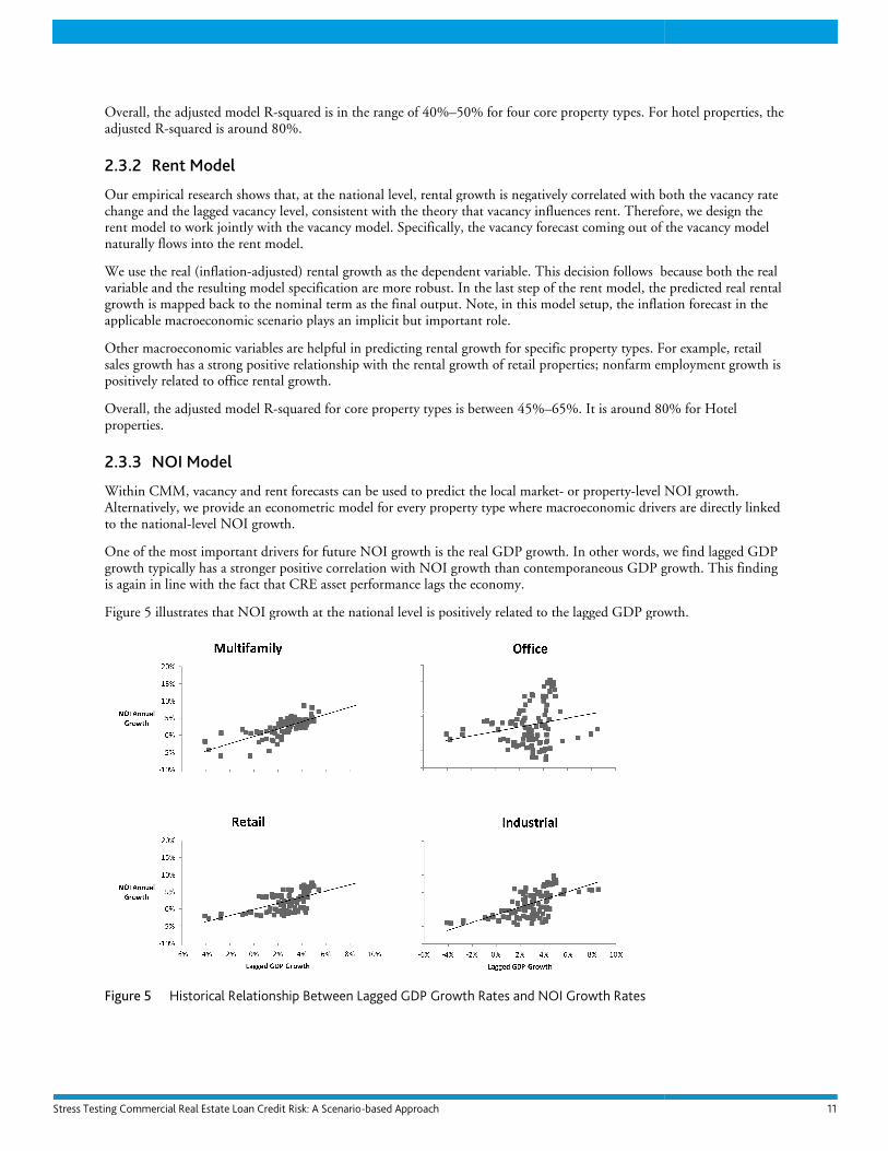
2.3.3 NOI Model

Within CMM, vacancy and rent forecasts can be used to predict the local marketAlternatively, we provide an econometric model for every property type whto the national-level NOI growth.

One of the most important drivers for future NOI growth is the real GDP grgrowth typically has a stronger positive correlation with NOIis again in line with the fact that CRE asset performance lags the economy.

Figure 5 illustrates that NOI growth at the national level is positively related to the lagged GDP growth.

Figure 5 Historical Relationship Between

Scenario-based Approach

is in the range of 40%–50% for four core property types. For

Our empirical research shows that, at the national level, rental growth is negatively correlated with both the vacancy rate consistent with the theory that vacancy influences rent. Therefore, we design the

rent model to work jointly with the vacancy model. Specifically, the vacancy forecast coming out of the vacancy model

adjusted) rental growth as the dependent variable. This decision follows because both the real variable and the resulting model specification are more robust. In the last step of the rent model, the predicted real rental

the nominal term as the final output. Note, in this model setup, the inflation forecast in the applicable macroeconomic scenario plays an implicit but important role.

helpful in predicting rental growth for specific property types. For example, ales growth has a strong positive relationship with the rental growth of retail properties; nonfarm employment growth is

positively related to office rental growth.

squared for core property types is between 45%–65%. It is around 80% for Hotel

Within CMM, vacancy and rent forecasts can be used to predict the local market- or property-level NOI growth. Alternatively, we provide an econometric model for every property type where macroeconomic drivers are directly linked

One of the most important drivers for future NOI growth is the real GDP growth. In other words, we findgrowth typically has a stronger positive correlation with NOI growth than contemporaneous GDP growth. This is again in line with the fact that CRE asset performance lags the economy.

that NOI growth at the national level is positively related to the lagged GDP growth.

etween Lagged GDP Growth Rates and NOI Growth Rates

11

For hotel properties, the

Our empirical research shows that, at the national level, rental growth is negatively correlated with both the vacancy rate consistent with the theory that vacancy influences rent. Therefore, we design the

rent model to work jointly with the vacancy model. Specifically, the vacancy forecast coming out of the vacancy model

because both the real In the last step of the rent model, the predicted real rental

in this model setup, the inflation forecast in the

rty types. For example, retail etail properties; nonfarm employment growth is

It is around 80% for Hotel

level NOI growth. ere macroeconomic drivers are directly linked

owth. In other words, we find lagged GDP growth than contemporaneous GDP growth. This finding

that NOI growth at the national level is positively related to the lagged GDP growth.

12

The strength of the positive relationship varies by property type, with the multifamily sector being the strongest, the office sector being the weakest, and others falling in between. This finding may be attributable to the difference in their lease terms. On the one hand, multi-year office leases lock in rental income for the duration of the lease term, even if the office tenants’ actual space needs may decrease. On the other hand, the short lease term of apartments (usually one year) causes rental income to be much more sensitive to economic downturns or growth.

Examples of other significant macroeconomic indicators for NOI growth are unemployment rate, federal funds rate, inflation, and home price appreciation rate. The exact model specification varies by property type. In the case of the retail sector, we find its NOI growth is positively correlated with the home price appreciation. The majority of U.S. household wealth is tied to housing. The rise of home prices stimulates consumer spending, which boosts retail sales and retail property income.

2.3.4 Cap Rate Model

Capitalization rate (cap rate) is defined as a property’s annual NOI divided by the property’s value. Cap rate is used as a standard measure or benchmark for a property’s value based on current performance.

Cap rate also serves as an indicator of investor expectations. Similar to bond “yields,” which are how bond prices are quoted, cap rates are a way of quoting observed market prices for CRE assets. Our empirical research indicates a strong correlation between cap rates and 10-year Treasury yields. Using the univariate linear regression model, we can explain about 50% of the variability in the cap rates for multifamily, office, and industrial properties.

2.4 Local CRE Markets

The translation models above provide the national-level CRE market factors projected under a given macroeconomic scenario. Since real estate business is all about “location, location, location,” local CRE market information is crucial to the success of stress testing. Figure 6 compares historical rental growth in two metropolitan areas, Washington DC and San Francisco. Over the past two decades, office rental growth in Washington DC was much less volatile than in San Francisco, because the office market in Washington, DC is largely dominated by businesses catering to the federal government or it is used directly by the agencies; whereas, the San Francisco market is determined primarily by much more volatile industries such as technology and financial services.

Figure 6 Historical Office Rent Growth Rates

After obtaining the national-level CRE market forecast, the second step in our “translation” process applies the national-level market factors to the local market factors. To capture local market dynamics, we leverage expertise from CBRE EA, which provides property type specific forecasts at the metropolitan and submarket levels for most of the active U.S.

-30%

-20%

-10%

0%

10%

20%

30%

'91 '92 '93 '94 '95 '96 '97 '98 '99 '00 '01 '02 '03 '04 '05 '06 '07 '08 '09 '10

Washington DC San Francisco


commercial real estate markets. We estimate local CRE market performance using the current local market condition and the relative rankings forecasted by CBRE EA under its Baseline Forecast.

4

2.5 7BModel Validation

Model validation is both theoretical and empirical, and requires both expert judgment on the economic rationale and actual out-of-sample model predictiveness. Specifically, our model validation consists of several aspects. First, we make sure that the signs of model coefficients do not violate economic intuition. Second, a model robustness check is performed over sub-samples and across time. Last but not least, we conduct out-of-sample tests to validate model performance.

We next demonstrate model robustness check process using the NOI models as an example. For each property type, we estimate the NOI model coefficients using two different samples. The first sample is effectively the entire time series data through 2009Q4. The second sample is through 2007Q4, in which we intentionally leave out the two-year period (2008–2009). If the models are robust enough, we should observe the following patterns between the two sets of model coefficients:

• Both sets of coefficients are consistent in terms of both magnitude and sign.

• The statistically significant variables in one set remain so in the other set.

• Model R-squares are in a similar range.

Our models perform well according to the above criteria. In the out-of-sample test, we use the in-sample period (such as the one through 2007Q4) to estimate model coefficients, and then use the resulting model to predict the CRE market factors over the out-of-sample period (such as 2008–2009). We find the overall out-of-sample model fitness satisfactory. Figure 7 shows a close fit between the predicted NOI growth rates and the actual NOI growth rates for the multifamily property type at the national level.

Figure 7 Model-Predicted NOI Growth Rates vs. Actual NOI Growth Rates

4 It is possible that the relative rankings will be different under different economic scenarios. To obtain the rankings “right” under

each new scenario, ideally one should conduct a rigorous modeling exercise that analyzes the potentially different market response under the new economic scenarios. The downside of this “ideal” approach is that it is quite involved, with uncertain benefits. A key question is: whether we aim for “roughly right,” on time or “belatedly precise,” passing a decision timeframe? We believe that the former is more useful and actionable. Through our research, we also find that our approach works quite well for a reasonably diversified portfolio not concentrated in one or two locations.

-3.0%

-2.0%

-1.0%

0.0%

1.0%

2.0%

3.0%

-8.0% -6.0% -4.0% -2.0% 0.0% 2.0% 4.0%

Predicted NOI

Growth

Actual NOI Growth

14

However, the slope of the regression line in the above scatter plot is lower than 1. It implies that regression models lead to “under-prediction,” which has serious consequences in stress testing. It is worthwhile investigating why the “under-prediction” occurs. In developing macroeconomic scenario-based models, we try to predict the CRE asset performance using only macroeconomic variables. In fact, there are variables other than macroeconomic variables that influence CRE asset performance. The omitted variables give rise to “under-prediction.”

Let us consider a simplified example where GDP growth is used to forecast NOI growth. Since the model R-squared is lower than 100%, the variability of NOI growth cannot be fully explained by GDP growth. Consequently, as illustrated in Figure 8, a very stressed GDP growth input (e,g., at the 1% stress level) leads to a not-so-stressed NOI growth forecast (e.g., at the 15% stress level).

Figure 8 Problem of Under-estimation: Unintended Consequence of Scenario-Based Stress Testing

We designed customizable functions in CMM to correct for the problem of “under-prediction”. The higher the model R-squared is, the less need for the correction. Going back to the out-of-sample test example above, the regression model without correction predicts around -4% NOI growth for the multifamily property type at the market trough (late 2009), while the actual NOI growth was around -6%. After correction is applied, the final prediction becomes very close to the actual.

3 Implementation of Scenarios In this section, we use the scenarios available in December 2011 to explain how macroeconomic scenarios and CRE market forecasts are implemented within Moody’s CMM. We describe the assumptions and economic rationale behind this rich array of alternative scenarios. In sum, Moody’s CMM implements scenarios in six ways:

• CRE market scenarios formulated by Moody’s Analytics. These can be used as reference scenarios. For example, a no-growth scenario assumes no future changes in current vacancy, rent, NOI, cap rate, and price levels.

• CRE market forecasts provided by CBRE Econometric Advisors, an established expert in forecasting commercial real estate market performance. These are expert opinions formulated by CBRE EA regarding the most likely future for CRE local markets. CBRE EA also provides a few alternative scenarios as well.

• Macroeconomic forecasts and alternative scenarios as provided by Moodys’ Analytics. Typically seven macroeconomic scenarios, including a baseline, with some stronger growth and some weaker growth scenarios.


• Supervisory scenarios as specified by the Federal Reserve System. For example, the 2012 CCAR offers two supervisory scenarios: a baseline and a more adverse scenario.

• Historical scenarios. CMM users can change the analysis “as of” date to see how their portfolios would have performed should some actual CRE market events happen in the future. Albeit driven by somewhat different forces each time, market cycles do persist and history tends to repeat itself in various shapes or forms. The historical scenario analysis is a very intuitive and effective way to stress credit risks under the most realistic scenarios – because these scenarios are not hypothetical, they occurred before in the real world.

• Custom CRE market forecasts. Users can provide their own CRE market-specific scenarios and load them into the CMM system to conduct more extensive and user-defined analyses.

Below, we describe the assumptions for the scenarios formulated by Moody’s Analytics and the Federal Reserve.

3.1 7BCRE Market Scenarios Formulated by Moody’s Analytics

To help users get a benchmark understanding of the current market situation and to compare credit performance under a typical growing economic environment and a stressed market crash scenario, we developed three sets of reference CRE market scenarios.

No-Growth Scenario

Under this scenario, we assume no-growth (i.e. zero future growth rates) in the levels of CRE market factors: vacancy, rent, NOI, cap rate, and price. The main purpose of this scenario is to provide a reference point where users can disentangle the effect of future market movements from current market conditions. For example, under a recovery scenario where real estate income and prices are both expected to grow, the conditional credit risks would be measured lower. It is not easy for users to know how much of the lower credit risk estimates is due to expected income and price growth and how much is due to the current loan structure in terms of DSCR and LTV. The credit risk estimates from the no-growth scenario serve as a reference point from which users can compare the results, i.e. if an EDF credit measure for the same loan is estimated to be lower in scenario X compared with that in the no-growth scenario, then scenario X

must assume positive future growth rates in real estate income and/or price. On the other hand, if the EDF measure is estimated to be much higher in scenario Y, then scenario Y must assume quite negative growth rates in real estate income and/or price.

Mean-Reverting Scenario

Under this scenario, we assume the key CRE market factors gradually revert back to their historical mean from the current state. The exact magnitude or timing of changes in these factors may differ across property types. We illustrate the concept using examples from the multifamily sector.

Three CRE market factors (vacancy rate, rental growth and NOI growth) share the same set of assumptions. Starting from the analysis as of date, they evolve under the following assumptions:

• Within Year 1: the market factors stay at the current state. The reason for this assumption is to capture the stickiness of the commercial real estate market.

• Between Year 2 and Year 3: the market factors steadily revert back to the historical mean.

• After Year 3: the market factors remain at the historical mean.

The following figures show how these CRE factors move in the future for the Los Angeles multifamily market. We also plot the historical period for comparison.

16

Figure 9 Market Vacancy Rate in the “Mean-Reverting” Scenario

Figure 10 NOI and Rent Growth in the “Mean-Reverting” Scenario

The market price growth is assumed to follow these assumptions:

• Within Year 1: market price steadily reverts back to its historical mean growth rates. The reason for a quick mean-reverting process for CRE market price is to capture the working of the highly forward-looking and rapidly responsive capital markets.

• After Year 1: it remains at the historical mean.

Figure 11 Growth Rates of Market Price Index in the “Mean-Reverting” Scenario

0%

1%

2%

3%

4%

5%

6%

7%

8%

88 89 90 91 92 93 94 95 96 97 98 99 99 00 01 02 03 04 05 06 07 08 09 10 10 11 12 13 14 15 16

History Future

-15%

-10%

-5%

0%

5%

10%

15%

20%

88 89 90 91 92 93 94 95 96 97 98 99 99 00 01 02 03 04 05 06 07 08 09 10 10 11 12 13 14 15 16

NOI Growth (Annual) Rent Growth (Annual)

History Future

-40%

-30%

-20%

-10%

0%

10%

20%

30%

40%

50%

60%

88 89 90 91 92 93 94 95 96 97 98 99 99 00 01 02 03 04 05 06 07 08 09 10 10 11 12 13 14 15 16

Price Growth (Annual)

History Future


Please note, the cap rate movement can be inferred from the market-level NOI and price movements under the mean-reverting scenario.

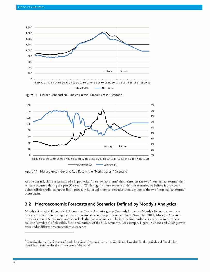
Market-Crash Scenario

This scenario is designed for estimating the upper end of credit losses under extreme, adverse market events while still maintaining its real-world plausibility into the foreseeable horizon. It emulates the worst historical experiences that occurred during the two “market crash” episodes in the last 30+ years: the late 1980s through early 1990s and the late 2000s (two “near-perfect storms” in our terminology). While heavily drawing upon actual experience in terms of the magnitude and patterns of changes in vacancy, rent, NOI, cap rate, and market price during these adverse periods, the scenario itself is a rather draconian setup. The key assumptions under this scenario:

• Local market vacancy. Over the next three years, the vacancy rate increases by a magnitude of two standard deviations from the current state. The increase throughout the three -year period is at a constant speed. In other words, the vacancy rate increases by the same amount in each quarter or year. The vacancy rate remains at the same level afterwards. The three -year gradual increase reflects the stickiness of the CRE space market and associated historical evidence.

• Local market rent index. Over the next three years, the rent index decreases by 20% from the current state. The decline is at a constant speed within the three-year period. After that, the rent index remains flat. The 20% rent decline is taken from examining the worst periods from the historical data series provided by CBRE EA.

• Local market NOI index. Over the next 30 quarters (or 7.5 years), the NOI index decreases by 30%. The decline is at a constant speed over the 30 quarters, after which the NOI index does not change. The 30% decline is consistent with that reported by the NCREIF from the mid-1980s through the mid-1990s.

• Local market cap rate. Over five years, the market cap rate is 1.3 times the current cap rate level. The increase is at a constant speed over the five years. After that, cap rates remain constant.

The following figures illustrate how these CRE factors play out in the Market-Crash Scenario. Again, we use the Los Angeles multifamily market as an example. Historical data is also shown. Note, the price movement can be implied from the NOI and cap rate evolutions as described above.

Figure 12 Vacancy Rate in the “Market Crash” Scenario

0%

1%

2%

3%

4%

5%

6%

7%

8%

9%

88 89 90 91 92 93 94 95 96 97 98 99 99 00 01 02 03 04 05 06 07 08 09 10 10 11 12 13 14 15 16

History Future

18

Figure 13 Market Rent and NOI Indices in the “Market Crash” Scenario

Figure 14 Market Price index and Cap Rate in the “Market Crash” Scenario

As one can tell, this is a scenario of a hypothetical “near-perfect storm” that references the two “near-perfect storms” that actually occurred during the past 30+ years.

5 While slightly more extreme under this scenario, we believe it provides a

quite realistic credit loss upper-limit, probably just a tad more conservative should either of the two “near-perfect storms” occur again.

3.2 7BMacroeconomic Forecasts and Scenarios Defined by Moody’s Analytics

Moody’s Analytics’ Economic & Consumer Credit Analytics group (formerly known as Moody’s Economy.com) is a premier expert in forecasting national and regional economic performance. As of November 2011, Moody’s Analytics provides seven U.S. macroeconomic outlook alternative scenarios. The idea behind multiple scenarios is to provide a realistic “envelope” of plausible, future realizations of the U.S. economy. For example, Figure 15 shows real GDP growth rates under different macroeconomic scenarios.

5 Conceivably, the “perfect-storm” could be a Great Depression scenario. We did not have data for this period, and found it less

plausible or useful under the current state of the world.

0

200

400

600

800

1,000

1,200

1,400

1,600

1,800

88 89 90 91 92 93 94 95 96 97 98 99 00 01 02 03 04 05 06 07 08 09 10 11 12 13 14 15 16 17 18 19 20

Rent Index NOI Index

History Future

0%

1%

2%

3%

4%

5%

6%

7%

8%

9%

0

20

40

60

80

100

120

140

160

88 89 90 91 92 93 94 95 96 97 98 99 00 01 02 03 04 05 06 07 08 09 10 11 12 13 14 15 16 17 18 19 20

Value Index (L) Cap Rate (R)

History Future


Figure 15 Real GDP growth patterns under alternative macroeconomic scenarios

Baseline Scenario (“S0”)

This scenario is the economy’s most likely future path opined by macroeconomists from Moody’s Analytics. The forecast embodies expert opinions, synthesizing the most liable current information and historical patterns. The baseline scenario is considered one of the Blue Chip economic forecasts in the U.S.

Table 2 Key Assumptions: Baseline (“S0”), November 2011

Variable 2011 2012 2013 2014 2015

GDP Change (%AR) 1.8 2.6 3.5 4.0 3.6

Unemployment Rate % 9.0 9.0 8.5 7.0 5.9

Median Existing-House Price (Change %YA) -4.7 -1.0 2.2 8.4 7.1

Inflation %AR 3.1 2.0 2.4 2.9 2.4

Federal Funds Rate % 0.1 0.0 0.3 1.7 3.4

Treasury Yield: 10-Year Bond % 2.8 3.5 4.9 4.6 4.6

S&P 500 Change 12.6 5.8 4.7 5.1 2.6

Stronger Near-Term Rebound Scenario (“S1”)

This above-baseline scenario is designed with a 10% probability that the economy will perform better than in this scenario, broadly speaking, and a 90% probability that it will perform worse.

Table 3 Key Assumptions: Stronger Near-Term Rebound Scenario (“S1”), November 2011

Variable 2011 2012 2013 2014 2015

GDP Change (%AR) 1.9 3.6 3.6 3.4 3.0


Median Existing-House Price (Change %YA) -4.6 1.1 2.1 6.2 7.2

Inflation %AR 3.2 2.3 2.4 2.7 2.3



S&P 500 Change 13.0 7.9 2.9 4.4 2.6

-4

-2

0

2

4

6

2011 2012 2013 2014 2015

Real GDP Growth

Rate (%)

S0: Baseline Forecast Summary S1: Stronger Near-Term Rebound

S2: Mild Second Recession S3: Deep Second Recession

S4: Protracted Slump S5: Below-Trend Long-Term Growth

S6: Oil Price Increase, Dollar Crash Inflation

20

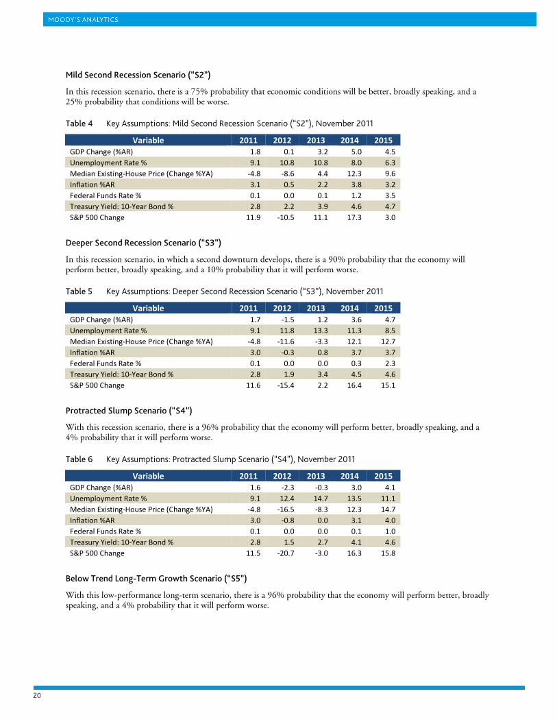
Mild Second Recession Scenario (“S2”)

In this recession scenario, there is a 75% probability that economic conditions will be better, broadly speaking, and a 25% probability that conditions will be worse.

Table 4 Key Assumptions: Mild Second Recession Scenario (“S2”), November 2011

Variable 2011 2012 2013 2014 2015

GDP Change (%AR) 1.8 0.1 3.2 5.0 4.5



Inflation %AR 3.1 0.5 2.2 3.8 3.2



S&P 500 Change 11.9 -10.5 11.1 17.3 3.0

Deeper Second Recession Scenario (“S3”)

In this recession scenario, in which a second downturn develops, there is a 90% probability that the economy will perform better, broadly speaking, and a 10% probability that it will perform worse.

Table 5 Key Assumptions: Deeper Second Recession Scenario (“S3”), November 2011

Variable 2011 2012 2013 2014 2015

GDP Change (%AR) 1.7 -1.5 1.2 3.6 4.7


Median Existing-House Price (Change %YA) -4.8 -11.6 -3.3 12.1 12.7

Inflation %AR 3.0 -0.3 0.8 3.7 3.7



S&P 500 Change 11.6 -15.4 2.2 16.4 15.1

Protracted Slump Scenario (“S4”)

With this recession scenario, there is a 96% probability that the economy will perform better, broadly speaking, and a 4% probability that it will perform worse.

Table 6 Key Assumptions: Protracted Slump Scenario (“S4”), November 2011

Variable 2011 2012 2013 2014 2015

GDP Change (%AR) 1.6 -2.3 -0.3 3.0 4.1



Inflation %AR 3.0 -0.8 0.0 3.1 4.0



S&P 500 Change 11.5 -20.7 -3.0 16.3 15.8

Below Trend Long-Term Growth Scenario (“S5”)

With this low-performance long-term scenario, there is a 96% probability that the economy will perform better, broadly speaking, and a 4% probability that it will perform worse.


Table 7 Key Assumptions: Below Trend Long-Term Growth Scenario (“S5”), November 2011

Variable 2011 2012 2013 2014 2015

GDP Change (%AR) 1.8 1.8 2.6 3.4 3.1



Inflation %AR 3.1 1.5 2.2 2.8 2.3



S&P 500 Change 12.3 1.1 3.9 4.9 5.1

Oil Price Increase, Dollar Crash Inflation Scenario (“S6”)

With this stagflation scenario, there is a 90% probability that the economy will perform better, broadly speaking, and a 10% probability that it will perform worse.

Table 8 Key Assumptions: Oil Price Increase, Dollar Crash Inflation Scenario (“S6”), November 2011

Variable 2011 2012 2013 2014 2015

GDP Change (%AR) 1.8 1.3 -1.6 2.7 5.2



Inflation %AR 3.2 3.8 3.7 1.7 1.7



S&P 500 Change 11.7 -2.7 -8.6 18.8 13.0

3.3 Supervisory Scenarios Specified by the Federal Reserve System

On Nov.22, 2011, the Federal Reserve System published “Comprehensive Capital Analysis and Review,” which laid out the guidelines on the new round of stress testing, namely CCAR 2012. The following description of both supervisory scenarios is quoted from the instruction package:

“The scenarios show quarterly trajectories for key macroeconomic and financial variables. Broadly speaking, the Supervisory Baseline scenario follows the consensus outlook from the Blue Chip Economic Indicators and other sources as of mid-November. The supervisory stress scenario features a deep recession that begins in the fourth quarter of 2011, in which the unemployment rate increases by an amount similar to that experienced, on average, in severe recessions such as those in 1973–1975, 1981–82, and 2007–2009, with a sizable shortfall in U.S. economic activity and employment, accompanied by a notable decline in global economic activity. The scenario also includes hypothetical asset price declines and risk premia increases that are designed, for the purposes of this exercise, to start in the fourth quarter of 2011.”

22

Table 9 Supervisory Baseline Assumptions: Selected Key Variables

OBS

Real

GDP

Growth

Real

Disposable

Income

Growth

Unemployment

Rate

CPI

Inflation

Rate

3-Month

Treasury

Yield

10-Year

Treasury

Yield

House

Price

Index

Commercial

Real Estate

Price Index

Q32011 (actual) 2.5 -1.7 9.1 3.1 0.0 2.5 136.9 174.1

Q42011 2.3 -0.5 9.1 1.9 0.1 2.2 137.2 172.2

Q12012 1.9 1.6 9.1 2.0 0.1 2.3 137.6 173.3

Q22012 2.2 2.1 9.0 1.9 0.1 2.4 137.9 175.4

Q32012 2.4 2.0 8.9 2.2 0.1 2.6 138.2 177.7

Q42012 2.6 2.4 8.9 2.1 0.1 2.8 138.6 178.9

Q12013 2.7 2.8 8.7 2.1 0.1 3.1 138.9 182.3

Q22013 2.8 2.9 8.5 2.3 0.1 3.3 139.3 185.6

Q32013 2.9 3.0 8.3 2.4 0.1 3.5 139.6 189.1

Q42013 3.0 3.0 8.1 2.4 0.6 3.7 140.0 192.6

Q12014 2.9 3.0 7.9 2.4 1.0 3.9 140.3 195.5

Q22014 3.0 3.1 7.8 2.4 1.4 4.0 140.7 198.6

Q32014 3.0 3.1 7.6 2.4 1.9 4.2 141.0 201.8

Q42014 2.9 3.1 7.5 2.4 2.3 4.3 141.4 205.0

Table 10 Supervisory Stressed Scenario Assumptions: Selected Key Variables

OBS

Real

GDP

Growth

Real

Disposable

Income

Growth

Unemployment

Rate

CPI

Inflation

Rate

3-Month

Treasury

Yield

10-Year

Treasury

Yield

House

Price

Index

Commercial

Real Estate

Price Index

Q32011 (actual) 2.5 -1.7 9.1 3.1 0.0 2.5 136.9 174.1

Q42011 -4.8 -6.0 9.7 1.9 0.1 2.1 135.1 168.4

Q12012 -8.0 -6.8 10.6 2.0 0.1 1.9 131.6 161.0

Q22012 -4.2 -4.3 11.4 1.9 0.1 1.8 127.5 153.4

Q32012 -3.5 -3.2 12.2 2.2 0.1 1.7 123.1 146.5

Q42012 0.0 -0.6 12.8 2.1 0.1 1.8 119.1 139.4

Q12013 0.7 0.7 13.0 2.1 0.1 1.7 115.2 136.8

Q22013 2.2 1.7 13.1 2.3 0.1 1.8 111.9 135.2

Q32013 2.3 2.7 13.0 2.4 0.1 2.0 109.8 134.0

Q42013 3.5 2.3 12.8 2.4 0.1 2.0 108.5 134.4

Q12014 3.4 2.8 12.6 2.4 0.1 2.0 108.1 134.5

Q22014 3.7 3.5 12.4 2.4 0.1 1.9 108.4 135.9

Q32014 4.6 2.8 12.0 2.4 0.1 1.9 109.2 139.5

Q42014 4.6 4.5 11.7 2.4 0.1 1.9 110.3 143.4

3.4 Historical Scenario Analysis

Historical scenario analysis is particularly interesting and useful. We define this type of stress testing basically by asking some simple and intuitive questions:

• What if the Great Recession of 2008-2009 happens again?

• What if the Great Depression of the 1930s happens again?

• What if the prolonged CRE market decline from the late 1980s through early the 1990s happens again?


These questions and answers can be easily understood by business users, and can be quite effectively communicated and explained across management and business units. Because we base the analysis upon past, realized market cycles, the results tend to be highly accurate and realistic (if the credit risk model is calibrated correctly), relating directly to the real-life experience of market participants. An additional appeal of this approach is the ease of execution, as long as one has enough historical data and robust enough software.

Figure 16 shows the historical scenario analysis process, assuming a loan was originated in 1980 with DSCR of 1.20 and LTV of 70% at origination. As we can see, as the commercial real estate market rose through 1985 and then gradually declined, the underlying collateral’s financial performance also likely first improved and then deteriorated corresponding with the market cycle. For such a loan, the cumulative 10-year PD would be 10.4% under the historical episode of 1980–1990.

Figure 16 Flowchart of Historical Scenario Analysis

We can then run multiple scenarios beginning with a different historical period. Table 11 shows a summary of cumulative PDs using historical scenarios starting in 1980. We stop at starting year of 2000 because we need a full 10-year realized history through 2010 for this type of exercise.

Table 11 Cumulative PD for a hypothetical loan: 1.20 DSCR and 70% LTV at origination

1 2 3 4 5 6 7 8 9 10

1980 0.2% 0.6% 1.2% 2.0% 2.8% 3.6% 4.8% 6.3% 8.2% 10.4%

1981 0.2% 0.6% 1.4% 2.3% 3.3% 4.6% 6.3% 8.5% 11.2% 14.7%

1982 0.3% 1.0% 2.1% 3.6% 5.4% 7.7% 10.4% 13.9% 18.8% 23.7%

1983 0.3% 1.1% 2.6% 4.8% 7.4% 10.4% 14.1% 19.3% 25.4% 29.1%

1984 0.3% 1.1% 2.9% 5.3% 8.3% 11.8% 16.9% 22.8% 27.0% 29.5%

1985 0.3% 1.6% 4.1% 7.6% 11.6% 17.0% 23.2% 27.6% 30.6% 32.3%

1986 0.4% 1.9% 4.8% 8.8% 14.3% 20.3% 24.5% 27.4% 29.3% 30.6%

1987 0.5% 2.2% 5.5% 10.8% 16.8% 21.0% 23.7% 25.5% 27.1% 27.9%

1988 0.4% 2.1% 5.9% 11.2% 14.9% 17.4% 18.9% 20.3% 21.2% 21.7%

1989 0.5% 2.5% 6.7% 10.1% 12.5% 13.9% 15.2% 16.0% 16.5% 17.1%

1990 0.6% 3.0% 5.9% 8.2% 9.7% 10.9% 11.7% 12.2% 12.8% 13.2%

1991 0.8% 2.6% 4.6% 6.0% 7.3% 8.1% 8.6% 9.2% 9.7% 10.1%

1992 0.5% 1.7% 2.8% 4.0% 4.8% 5.2% 5.8% 6.3% 6.7% 7.4%

1993 0.4% 1.2% 2.3% 3.1% 3.6% 4.2% 4.7% 5.2% 6.0% 7.0%

1994 0.3% 1.1% 2.0% 2.6% 3.3% 3.9% 4.4% 5.4% 6.7% 7.7%

1995 0.4% 1.1% 1.7% 2.7% 3.4% 4.1% 5.3% 6.9% 8.3% 9.2%

1996 0.2% 0.6% 1.3% 2.0% 2.6% 3.6% 5.1% 6.5% 7.5% 8.1%

1997 0.2% 0.7% 1.5% 2.2% 3.5% 5.3% 6.9% 8.1% 9.0% 9.5%

1998 0.3% 0.9% 1.7% 3.4% 5.7% 7.7% 9.1% 10.1% 10.9% 12.3%

1999 0.2% 0.8% 2.3% 4.7% 7.0% 8.5% 9.5% 10.4% 12.1% 17.0%

2000 0.2% 1.4% 4.1% 6.9% 8.8% 10.1% 11.0% 13.1% 19.5% 22.2%

Origination

Year

Years since Origination

24

Suppose we have a portfolio. Included in it, we originate 100 commercial morexactly the same origination amount for each loanhistorical periods as shown in Figure 17.

Figure 17 Portfolio Default Rates for a

Another very useful result from the historical scenario analysis is the distribution of scenariorealized historical scenarios. Figure 18 shows Each distribution is based on 84 observations, with each observation correspondhypothetical cohort. We define a cohort quarterly cohorts starting from 1980Q1 through 2010Q4, giving a total of 84 cohorts. The results are quite revealingthat, by imposing a stricter underwriting criteriathe credit risks are indeed well-controlled for lowloan group never exceed 18%, even during the severe and prolonged CRE market crash during the late 1980s and early 1990s.

Figure 18 Distribution of “Realized” Default

6 High-risk loans are defined as loans with DSCR of 1.20 and

DSCR of 1.80 and LTV of 60% at origination.

0%

1%

2%

3%

4%

5%

19

81

19

82

19

83

19

84

19

85

19

86

19

87

19

88

19

89

19

90

19

91

Portfolio PD

a portfolio. Included in it, we originate 100 commercial mortgages each year from 1980 to 2010 with the same origination amount for each loan; we end up with a pattern of portfolio default rates during the

ates for a Hypothetical Portfolio Under Historical Scenarios

Another very useful result from the historical scenario analysis is the distribution of scenario-based conditional PD under shows the comparison of distributions between high-risk loans and low

Each distribution is based on 84 observations, with each observation corresponding to the cumulative 10 as a group of loans originated within the same quarter. We run the scenarios on

quarterly cohorts starting from 1980Q1 through 2010Q4, giving a total of 84 cohorts. The results are quite revealingthat, by imposing a stricter underwriting criteria, such as increasing requirement on DSCR and LTV at loan

controlled for low-risk loan groups. The cumulative 10-year default rates even during the severe and prolonged CRE market crash during the late 1980s and early

efault Rates Based upon Historical Scenarios

risk loans are defined as loans with DSCR of 1.20 and LTV of 70% at origination, and low-risk loans are defined as loans with DSCR of 1.80 and LTV of 60% at origination.

19

91

19

92

19

93

19

94

19

95

19

96

19

97

19

98

19

99

20

00

20

01

20

02

20

03

20

04

20

05

20

06

20

07

20

08

20

09

tgages each year from 1980 to 2010 with end up with a pattern of portfolio default rates during the

based conditional PD under risk loans and low-risk loans.

6

to the cumulative 10-year PD for a er. We run the scenarios on

quarterly cohorts starting from 1980Q1 through 2010Q4, giving a total of 84 cohorts. The results are quite revealing, in such as increasing requirement on DSCR and LTV at loan origination,

year default rates for the low-risk even during the severe and prolonged CRE market crash during the late 1980s and early

risk loans are defined as loans with

20

10


In sum, we find historical scenario analysis particularly useful for the CRE asset class, given that the CRE market experienced two extreme downturns during the past three decades, which provide some actual downside scenarios with real-world stories and meanings. In our opinion, scenario-based stress testing provides indispensible perspective and definitely deserves its place, complementing many other methods.

4 7BInterpreting and Making Use of the Results In this section, we compare the conditional credit risk estimates from alternative scenarios and offer some thoughts on interpreting and making use of the results.

Working as intended, it is straightforward and intuitive to interpret the credit risk measures under given macroeconomic scenarios. For example, a given stressed economic scenario leads to stressed PD and EL measures under that scenario. That said, it is critical to keep in mind some important statistical properties of the credit risk distribution to appreciate how one should interpret and make the best use of the results.

4.1 Interpreting Scenario-Based Results

A known statistical property of credit loss distribution is its right-hand skewed, fat-tail distribution. Credit losses cannot be negative while the upper limit is 100% of the exposure. In the meantime, credit events are rare events with low probability of happening, meaning the expected default frequency and expected loss is typically in the low single-digits (or less) measured on an annual frequency. This stylized pattern can be shown in Figure 19.

Figure 19 Credit Loss Distribution and Points of Median, Mean, and Stressed Percentiles

The graph depicts a distribution curve of conditional PD measures for a typical commercial mortgage, covering a full range of all possible economic scenarios. Each point on the curve corresponds to a conditional PD estimate for an underlying economic scenario. Note, this figure does not include the idiosyncratic variation; hence, one can also interpret it as representing the distribution of default rates for a very well-diversified portfolio of commercial mortgages when the single risk driver is the market/economy.

7 Notice the following important observations:

7 To help interpret the chart better, maybe it is easier to think of this as equivalent to a probability density plot of the returns of S&P

500 Index instead of a plot on an individual component such as Microsoft.

0% 5% 10% 15% 20% 25% 30% 35%

Density

10-year Cumulative PD

Median PD (corresponding to Baseline

economic forecast): 6.0%

Mean PD (probability-

weighted EDF): 8.7%

95th Percentile PD : 24.9%

roughly corresponding to

the CRE credit events

happened between late

1980s through early 1990s

26

• The Median PD, while usually corresponding to the baseline economic forecast, is almost always less than the unconditional expected default frequency (EDF credit measure) integrated from all possible economic scenarios. The importance of this statistical property: users should always be aware that the conditional PD and EL measures from a baseline scenario should not be used as if they were unconditional expected (mean) measures. Using conditional PD and EL measures from a baseline scenario, in fact, always understates the true risks, although the magnitude of such understatement varies by loan characteristics and market volatilities, among other things.

• For a typical commercial mortgage, it is possible that the unconditional expected (mean) measures of PD can be significantly higher than the median PD measure. Our example in Figure 19, which describes a typical mortgage, suggests that the unconditional expected PD measure can be 1.45 times the median measure. In other words, for the purposes of loss forecast, loss reserve, and loan pricing, users should use 1.45 times the median PD measure (i.e. PD estimated from a baseline economic forecast), if a PD from the baseline forecast is the only input into the decision process.

• The tail risk is “fat,” and default rates can be exponentially higher in a stressed economic environment. One should not use a normal distribution proxy as a shortcut. In our example, the 95

th-percentile conditional PD is measured at

24.9%, about four times the median PD and three times the mean PD. Such heavy tails on the right-hand side explain why the mean PD can be significantly higher than the median PD. From a business intuition perspective, the 95

th-percentile economic scenario roughly corresponds to the CRE credit events that happened between the late

1980s through the early 1990s, during which period the default rates and loss rates skyrocketed when the CRE market vacancy rates soured, leading to severe declines in rent, income and market price. This experience was somewhat echoed by the severe CRE market deterioration during the recent financial crisis, during which period commercial property prices dropped by more than 40%, accompanied by rising vacancy rates and declining rents. The two “market crash” events happened within a window of about 30 years, lasting a few years each, so a 95

th-

percentile is consistent with the history, in a broad sense.

4.2 Make Use of Scenario-Based Results

What does all this mean for a business user? We make several suggestions as rules of thumb based upon our observations of CMM model results and how typical users apply them in a business setting:

• Treat the PD/EL estimates from the Baseline forecast by CBRE EA (or by Moody’s Analytics) as the median risk measures, which tend to be lower than the mean (expected) measures.

• If the business needs are unconditional expected risk measures,8 then users have three options that are easy to

implement:

o Take a weighted-average PD/EL measure from several scenarios, including the “market crash” (i.e. “worst history”) scenario to ensure the tail risk is accounted for adequately. Our experiment also suggests that an EDF credit measure, calculated simply from a 90% weighted baseline forecast and a 10% weighted “market crash” scenario, is an adequate measure broadly in-line with the expected PD measure if one were to integrate all possible economic scenarios.

9 The same applies to EL as well.

o If the only input available is a PD/EL under the Baseline forecast (i.e. median PD/EL), then users should apply a multiplier of more than one to the median PD/EL to compensate for the fact that the unconditional expected PD/EL is almost always higher.

o In the current market environment, the conditional PD/EL measures, generated under the “no-growth” scenario, are also close enough to the expected, mean, PD/EL measures. We should point out that, while it is likely to work well currently and in the foreseeable near future as well, this approach may cease to work well if the CRE market were to enter a boom period.

8 In common business language, the unconditional expected PD measure is the one free of betting on a particular scenario while

recognizing the different probabilities across a baseline scenario, a double-dip recession scenario, a protracted slump scenario, etc. And it is also the one that takes into proper account the asymmetric fat tail losses under the less likely, yet severely damaging, economic environments. 9 While possible within CMM, users may quickly realize that it is rather difficult, if not entirely impossible, to assign a probability to a

market scenario, preventing the exercise of the integration of full ranges. Thus, our quick rules of thumb, in fact, turns out to be quite cost-effective with little loss of accuracy.


We use an example to illustrate how we should make intelligent use of the scenario-based risk measures. Table 12 and Figure 20 show the cumulative EDF and EL measures from 2012 to 2014, respectively, for a sample commercial mortgage portfolio under various economic scenarios specified by the Federal Reserve and Moody’s Analytics. The starting point is the end of 2011, so the estimates are for new defaults and losses on these new defaults expected to occur between 2012 and 2014. The actual recognized losses can be higher because the existing delinquencies and defaults will also have loss rates not included in Table 12.

Table 12 Cumulative PD Measures under Various Economic Scenarios

Cumulative PD

line Years 2012 2013 2014

Federal Reserve Scenarios

a) CCAR 2012 Base 1.18% 2.07% 2.87%

b) CCAR 2012 Stress 3.66% 7.69% 9.96%

Moody's Analytics Reference CRE Market Scenarios

c) No Growth Scenario 1.10% 2.07% 3.01%

d) CRE Market Crash 2.28% 5.11% 8.62%

Moody's Analytics Macroeconomic Scenarios

e) MEDC Baseline 1.69% 2.56% 3.33%

f) Stronger Near-Term Rebound 1.21% 1.90% 2.50%

g) Mild Second Recession 2.33% 3.02% 3.93%

h) Deeper Second Recession 2.83% 4.58% 5.45%

i) Protracted Slump 3.32% 5.94% 7.04%

j) Oil Price Increase, Dollar Crash, Inflation 1.20% 4.43% 6.17%

k) Below-trend Long-term Growth 1.22% 2.35% 3.50%

l) Weighted by probability of all scenarios

10 1.90% 2.98% 3.84%

m)

90% weighted MEDC Baseline and 10%

weighted CRE Market Crash 1.75% 2.82% 3.86%

The Federal Reserve CCAR 2012 stressed scenario assumes very severe and rapid near-term economic declines, leading to even higher near-term credit loss estimates than our draconian “market crash” scenario that assumes a more gradual and prolonged market decline. For example, real GDP decline of 8% in the middle of 2012 is a rather strong assumption. Given the currently fragile CRE market environment, we expect a highly adverse outcome if that scenario occurs. Under the stressed scenario, the credit losses would very likely outpace the levels experienced during the recent financial crisis, given that the CRE markets have lost most financial cushions and are very vulnerable already from the market deterioration during the past few years.

10

Weighted results of all seven Moody’s Analytics macroeconomic scenarios where the weights are assigned by the probability of each scenario happening according to the descriptive guidance provided by Moody’s Analytics’ Economic and Consumer Credit Analytics Group. While there are infinite numbers of future economic paths, and the seven scenarios are just a few of possible realizations, theoretical arguments aside, these seven scenarios provide a good enough, discrete approximation to the infinite range of future paths, particularly for the near term (within three–five years’ horizon).

28

Figure 20 Cumulative Credit Loss Estimates Under Representative Scenarios

The distribution of expected losses under different scenarios as shown in Figure 20 also reflects our earlier point that credit losses tend to have fat tails, that is, even though a stressed economic scenario is less likely to happen, the outcome can be exponentially, rather than linearly, increasing credit losses.

4.3 Concluding Remarks

Given the increased regulatory and internal risk management requirements for periodic stress tests, we have designed a scenario-based credit risk modeling approach that takes into account macroeconomic assumptions regarding GDP, unemployment, inflation, interest rates, etc. Since the composite modeling approach implemented by Moody’s CMM is much closer to a structural model, it is quite logical and natural to incorporate macroeconomic assumptions as the upstream inputs. We developed the linkage models that translate forward-looking macroeconomic assumptions into CRE market scenarios. Our empirical analysis, model validation, and real-time application suggest the approach works as designed and is well-positioned to answer the business questions around credit loss estimates under pre-defined macroeconomic scenarios, such as in the case of the Federal Reserve CCAR 2012 program.

Clearly, as we have reached a newer level of sophistication and accuracy regarding scenario analysis and stress testing, they also potentially open the door for unintended misinterpretation of the scenario-based risk measures. We hope this paper highlights the key areas requiring serious attention. As demonstrated throughout the paper, if one can skillfully harness its power, our scenario analysis and stress testing models provide quite accurate results, conditional upon certain economic scenarios, in a very cost-effective fashion.

0.0%

0.5%

1.0%

1.5%

2.0%

2.5%

3.0%

3.5%

4.0%

4.5%

5.0%

2011 2012 2013 2014

Fed CCAR 2012 Base

Fed CCAR 2012 Stress

MEDC Baseline

Mild Second Recession

Deeper Second Recession

Protracted Slump


References

Acknowledgements

The authors thank substantive feedbacks and comments from our clients and regulators.

Copyright © 2011 Moody's Analytics, Inc. and/or its licensors and affiliates. All rights reserved.

References

Chen, Jun and Jing Zhang, 2011, “Modeling Commercial Real Estate Loan Credit Risk: An Overview,” Moody’s Analytics white paper, 2011.

Chen, Jun, Kevin Cai and Jing Zhang, 2011, “Modeling Commercial Real Estate Loan Credit Risk,” Moody’s Analytics white paper, 2011.

Federal Reserve System, 2009, “The Supervisory Capital Assessment Program: Design and Implementation,” April 24, 2009

Federal Reserve System, 2009, “The Supervisory Capital Assessment Program: Overview of Results,” May 7, 2009

Federal Reserve System, 2011, “Comprehensive Capital Analysis and Review: Objectives and Overview,” March 18, 2011

Federal Reserve System, 2011, “Comprehensive Capital Analysis and Review: Summary Instructions and Guidance,” November 22, 2011

Moody’s Analytics, 2011, “U.S. Macroeconomic Outlook Alternative Scenarios,” November 2011.

Office of the Comptroller of the Currency, 2006, “Concentrations in Commercial Real Estate Lending, Sound Risk Management Practices,” Department of the Treasury, Docket No. 06-14, 2006.

Stein, Roger M., 2011, “The Role of Stress Testing in Credit Risk Management,” Working Paper, Moody’s Research Labs, 2011.

stress testing cre credit risk a scenario approach€¦ · stress testing commercial real estate...

Documents