1

STRESS ANALYSIS OF COMPOSITE CYLINDRICAL SHELLS WITH AN

ELLIPTICAL CUTOUT

E. Oterkus, E. Madenci

Department of Aerospace and Mechanical Engineering

The University of Arizona, Tucson, AZ 85721

M. P. Nemeth

Mechanics of Structures and Materials Branch

NASA Langley Research Center, Hampton, VA 23681

Abstract

A special-purpose, semi-analytical solution method for determining the stress and

deformation fields in a thin laminated-composite cylindrical shell with an elliptical cutout is

presented. The analysis includes the effects of cutout size, shape, and orientation; non-uniform

wall thickness; oval-cross-section eccentricity; and loading conditions. The loading conditions

include uniform tension, uniform torsion, and pure bending. The analysis approach is based on

the principle of stationary potential energy and uses Lagrange multipliers to relax the kinematic

admissibility requirements on the displacement representations through the use of idealized

elastic edge restraints. Specifying appropriate stiffness values for the elastic extensional and

rotational edge restraints (springs) allows the imposition of the kinematic boundary conditions in

an indirect manner, which enables the use of a broader set of functions for representing the

displacement fields. Selected results of parametric studies are presented for several geometric

https://ntrs.nasa.gov/search.jsp?R=20080006848 2018-05-18T23:04:29+00:00Z

2

parameters that demonstrate that analysis approach is a powerful means for developing design

criteria for laminated-composite shells.

Introduction

Cutouts in cylindrical shell-type components are unavoidable in the construction of

aerospace structures. This fact is significant because the structural failure of these components

usually begins near the cutout because of high stress concentrations that initiate the formation of

cracks. Hence, a cutout can trigger a local failure at a load level lower than the global failure

load of a corresponding shell without a cutout. As a result, preliminary-design sizing of a

cylindrical shell with a cutout is often based on the magnitude of the stress concentrations near

the cutout. Therefore, an accurate assessment of the stress concentrations in a given shell

subjected to various types of loading and support conditions is essential to the development of

safe and reliable designs. Moreover, validated special-purpose analysis tools that enable rapid

parametric studies would be very valuable to structural designers and for the development of new

design criteria and design concepts.

Several analytical, numerical and experimental studies have been conducted during the past

sixty years to determine stress distributions in cylindrical shells with a cutout and subjected to

various types of loadings; such as, axial tension and compression, torsion, and internal and

external pressure. Pioneering analytical work was conducted by Lurie1,2 to investigate the effect

of axial tension and internal pressure, and shell curvature, on the stress concentrations around a

circular cutout in the 1940s. Many years later, analytical studies were presented by

Lekkerkerker,3 Van Dyke,4 Ashmarin,5 Murthy et al.,6 Guz et al.,7 and Van Tooren et al.8 that

further investigated the effects of various factors on the stress concentrations around a cutout in a

3

cylindrical shell. Similarly, experimental investigations have been conducted by Tennyson,9

Starnes,10 Pierce and Chou,11 Bull,12 and Zirka and Chernopiskii,13 and numerical studies have

been conducted by Liang et al.,14 and Shnerenko and Godzula.15 In 1964 and 1972, respectively,

Hicks16 and Ebner and Jung17 summarized the results obtained from several of these previous

studies and provided extensive lists of references related to this problem. Most of these previous

studies are for isotropic cylindrical shells with a circular cutout. Only a few of these studies, such

as those presented by Pierce and Chou11 and by Murthy et al.,6 address the effects of cutout shape

(elliptical cutouts) on the stress concentrations.

Mitigation of high stress concentrations by tailoring shell-wall thickness, material orthotropy

and anisotropy, and cutout reinforcement are also important considerations in the design of

aerospace structures made of lightweight composite materials. Likewise, the potential for using

shells of non-circular cross section are relevant to fuselage-like structures. However, only a few

studies have considered these effects. For example, the influence of wall-thickness variation on

the stresses in axially loaded composite cylindrical shells, without a cutout, has been investigated

by Li et al.18 Although numerous analyses exist in the literature on the analysis of shells with

circular cross sections, only a few include non-circular cross sections. Sheinman and Firer19

provided an analytical investigation of stresses in laminated cylindrical shells with arbitrary non-

circular cross sections. More recently, Hyer and Wolford20,21 studied the effect of non-circular

cross sections on damage initiation and progressive failure in composite cylinders by employing

the finite element method.

The objective of the present study is to present a special-purpose analysis for a laminated-

composite cylindrical shell with an elliptical cutout that can be used to rapidly, and

parametrically, investigate the effects of shell curvature; cutout size, shape, and orientation; and

4

ply lay-up on stress-resultant concentrations near the cutout. The analysis is applicable to thin-

walled cylindrical shells with non-uniform wall thickness, a non-circular (e.g., oval) cross

section, and subjected to tension, torsion, and bending loads as illustrated in Fig. 1.

To accomplish this objective, an overview of the analysis is presented first. Next, the

boundary value problem is defined along with the kinematics and stress-strain relations used in

the analysis. Then, the derivation of the equations governing the response and numerical

procedure are described. Finally, selected numerical results for oval and circular cylindrical

shells with either circular or elliptical cutouts and subjected to either tension, torsion, or pure-

bending loads are presented.

Analysis Overview

The analytical approach used herein permits the determination of the pointwise variation of

displacement and stress components. It is based on the principle of stationary potential energy,

but utilizes local and global functions that are not required to satisfy the kinematic boundary

conditions directly. Thus, the choice of local and global functions is not limited by a particular

type of kinematic boundary condition. The kinematic boundary conditions are imposed by

employing the Lagrange multiplier method. Both local and global functions are used, in contrast

to the traditional approach, to enhance the robustness of the analysis method. In particular, the

local functions are used to capture rapidly varying stress and strain gradients and local

deformations near a cutout. Toward that goal, Laurent series are used for the local functions and

are expressed in terms of the mapping functions introduced by Lekhnitskii.22 Fourier series are

used for the global functions and are used to capture the overall deformation and stress fields.

The kinematic admissibility requirements on the local and global functions are relaxed by

5

defining that the edges of the shell are supported by extensional and rotational springs. Zero-

valued displacement and rotation kinematic boundary conditions are enforced in an indirect

manner by specifiying values for the spring stiffnesses that are large compared to the

corresponding shell stiffnesses. This approach effectively yields a prescribed kinematic

boundary condition in the limit as the relative stiffness of the spring becomes much greater than

the corresponding shell stiffness. Similarly, values for the spring stiffnesses can be selected that

correspond to a given uniform elastic restraint along an edge, similar to that provided by an end-

ring. This capability is important, and useful, because in some test fixtures or actual structures

the edge supports may not be stiff enough to simulate a fully clamped boundary condition or

flexible enough to simulate a simply supported boundary condition.

As suggested by Li et al.18 and Sheinman and Firer,19 nonuniform wall-thickness variations

of a shell, which lead to non-uniform laminate stiffnesses, are represented by using trigonometric

series. Specifically, nonuniform shell-wall thickness is represented in the present study by

perturbing the ply thicknesses with a function that is periodic in either the longitudinal or the

circumferential direction. The variation in wall thickness is accounted for by adjusting the

lamina properties, resulting in nonhomogeneous in-plane and bending stiffness matrices. The

nonuniform shell curvature associated with a noncircular cross section is represented by using

trigonometric series for the coordinates of an oval-cross-section shell reference surface.23 The

aspect ratio, or out-of-roundness, of the cross-section is represented in the analysis by using an

eccentricity parameter.

In the derivation of the equations governing the response, the total potential energy consists

of the elastic strain energy of the shell, the elastic edge restraints and the potential energy of the

applied loads. The conditions that may arise from the choice of displacement approximations

6

without any kinematic restrictions are treated as constraint equations, and the potential energy

arising from constraint reactions is invoked into the total potential energy through the use of

Lagrange multipliers. The equations governing the shell response are obtained by enforcing the

requirement that the first variation of the total potential energy vanish. The evaluation of the

area integrals appearing in the potential energy are achieved numerically by using a basic

quadrature method in conjunction with standard triangulation of the entire domain described by

Shewchuk.24 Solution to the equations governing the response are obtained by using a standared

Gaussian elimination procedure, which yields the generalized displacement coefficients and,

thus, the stress and strain fields. The accuracy of the analysis depends on the number of terms

used for the functional representation of the displacement fields. As the number of terms

increases, the results converge to the exact solution.

Representation of Shell Geometry

The geometry of a thin-walled, noncircular, cylindrical shell of length L and with an elliptical

cutout located at the shell mid-length is shown in Fig. 1. The origin of the global Cartesian

coordinate system, ( , , )x y z is located at an end point of the longitudinal axis of the shell. As

shown in Fig. 1, the x-axis coincides with the longitudinal axis of the shell. The y and z

coordinates span the cross-sectional plane. A curvilinear coordinate system is also attached to the

mid-surface of the cylindrical shell. The coordinates of points in the longitudinal, circumferential

(tangential), and normal-to-the-surface (transverse) directions of the shell are denoted by (s1, s2,

s3), and the corresponding unit base vectors are {e1, e 2, e 3}.

Following Romano and Kempner,23 the non-circular cross-section of the cylindrical shell is

defined as an oval with the coordinates, y and z expressed as

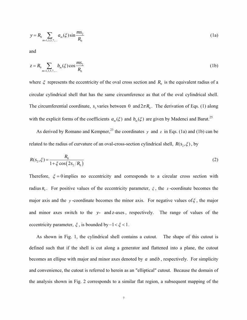
7

20

1,3,5,7, 0

( ) sinmm

msy R aR

ξ=

= ∑…

(1a)

and

20

1,3,5,7, 0

( ) cosmm

msz R bR

ξ=

= ∑…

(1b)

where ξ represents the eccentricity of the oval cross section and 0R is the equivalent radius of a

circular cylindrical shell that has the same circumference as that of the oval cylindrical shell.

The circumferential coordinate, 2s varies between 0 and 02 Rπ . The derivation of Eqs. (1) along

with the explicit forms of the coefficients ( )ma ξ and ( )mb ξ are given by Madenci and Barut.25

As derived by Romano and Kempner,23 the coordinates y and z in Eqs. (1a) and (1b) can be

related to the radius of curvature of an oval-cross-section cylindrical shell, 2( , )R s ξ , by

( )0

22 0

( , )1 cos 2

RR ss R

ξξ

=+

(2)

Therefore, 0ξ = implies no eccentricity and corresponds to a circular cross section with

radius 0R . For positive values of the eccentricity parameter, ξ , the z -coordinate becomes the

major axis and the y -coordinate becomes the minor axis. For negative values ofξ , the major

and minor axes switch to the -y and -axesz , respectively. The range of values of the

eccentricity parameter, ξ , is bounded by 1 1ξ− < < .

As shown in Fig. 1, the cylindrical shell contains a cutout. The shape of this cutout is

defined such that if the shell is cut along a generator and flattened into a plane, the cutout

becomes an ellipse with major and minor axes denoted by a andb , respectively. For simplicity

and convenience, the cutout is referred to herein as an "elliptical" cutout. Because the domain of

the analysis shown in Fig. 2 corresponds to a similar flat region, a subsequent mapping of the

8

ellipse to a unit circle is possible, which enables the use of Laurent series expansions for the

local functions. Note that the special case of a "circular" cutout is given by a b= .

In the flat analysis domain, the minor and major axes of the ellipse are aligned with a local

coordinate system, 1 2( , )x x , whose origin is located at the center of the cutout and coincides with

the origin of the parameter grid, given by constant values of s1 and s2, that forms the curvilinear

coordinates (s1, s2) on the cylindrical shell mid-surface. The orientation of the elliptical cutout is

arbitrary with respect to the longitudinal shell axis. Hence, the orientation of the local 1-x axis

(major axis) of the cutout and the longitudinal 1s -axis of the cylindrical shell is denoted by the

angle, ψ . The elliptical coordinates, α andβ , representing a family of confocal ellipses and

hyperbolas, respectively, are utilized in order to obtain the stress-resultant distribution in the

direction tangent to the cutout boundary. The coordinate α is equal to 10 tanh ( / )b aα −= on the

particular ellipse that corresponds to the elliptical cutout. The other coordinate, β , varying

from 0 to 2π , is known as the eccentric angle and is related to the 1 2( , )x x coordinate system by

1 cosx a β= and 2 sinx b β= . The eccentric angle β is similar to the angle used for polar

coordinates.

The symmetrically laminated cylindrical shells considered herein are made of K specially

orthotropic layers, and each layer has an orientation angle, kθ , that is defined with respect to the

1s -axis. Each layer also has elastic moduli LE and TE , shear modulus, LTG and Poisson’s

ratio LTν , where the subscripts L and T represent the longitudinal (fiber) and transverse

principal material directions, respectively.

9

As for the shell thickness variation, the non-uniform wall thickness of the shell is denoted

by 1 2( , )h s s , and its variation is included by assuming that the thickness of each ply, kt , varies as

a function of the curvilinear coordinates in the form

1 1 2 21 2 0 1 2

0

2( , ) 1k km s m st s s t Cos CosL R

πε ε⎞⎛ ⎞⎛ ⎛ ⎞= − − ⎟⎜ ⎟⎜ ⎟⎜ ⎟⎝ ⎠⎝ ⎝ ⎠⎠

(3)

where 0kt denotes the nominal thickness of the thk layer in the laminate, and the parameters

( 1 2,m m ) and ( 1ε , 2ε ) respectively, denote the wave numbers and the amplitudes of the periodic

thickness variation in the longitudinal and circumferential directions. While the wall thickness of

the shell is allowed to vary across the shell surface, the aspect ratio of the plies through the

thickness is maintained, thus making the thickness variation of each ply to remain conformable

to each other throughout the shell surface. A periodic thickness variation in the longitudinal

direction is obtained by setting 1 0ε ≠ and 2 0ε = , and in the circumferential direction by 1 0ε =

and 2 0ε ≠ . A shell with uniform thickness, 0k kt t= , is obtained by setting 1 0ε = and 2 0ε = .

Boundary Conditions and External Loads

To facilitate a general imposition of prescribed boundary tractions, displacements, or

rotations; the external as well as the internal edge boundary Γ of the shell is decomposed into

(1) (2) (3)Γ = Γ +Γ +Γ (4)

As shown in Fig. 1, (1)Γ and (2)Γ denote the external edge boundary of the cylindrical shell and

(3)Γ represents the traction-free internal edge boundary around the cutout. The unit vector

normal to an edge is represented byn . Throughout this paper, a variable with the superscript “*”

is treated as a known quantity, arising from the externally applied loads or from prescribed

10

displacements and rotations. Also, the subscripts n , s , and t denote the directions normal,

tangent, and transverse (through-the-thickness) to the boundary, respectively. The details of how

prescribed edge loads and displacements are imposed in the analysis are presented subsequently.

Prescribed edge loads

External loads are applied to a shell by specifying values for the positive-valued stress

resultants shown in Fig. 1. More precisely, the membrane loads applied to the th boundary

segment, ( )Γ , are given by

*11 nN t= (5a)

*12 sN t= (5b)

where N11 and N12 are the axial and shear stress resultants, respectively, defined in the

cylindrical coordinate system. Likewise, shell-wall bending loads that are applied to the th

boundary segment are given by

*11 nM m= − (6a)

* *11,1 12,2 ,22 2t sM M t m+ = − (6b)

where 11M and 12M are the pure-bending and twisting stress resultants, respectively, defined in

the cylindrical coordinate system. Moreover, the left-hand side of Eq. (6b) is the Kirchhoff shear

stress resultant of classical shell theory.

As a matter of convenience, the analysis is formulated to also permit the specification of

concentrated forces and moments that are transmitted to the ends of the shell as if through a rigid

end-ring, as shown in Fig. 3. Presently, the concentrated force *nP and the concentrated axial

11

torque *sP are included in the analysis. The force *

nP is simulated in the analysis by specifiying a

uniform distribution of the axial displacement, with the unknown magnitude nΔ , such that

( )

*11 nN d P

Γ

Γ =∫ (7a)

Likewise, the torque *sP is simulated by specifiying a uniform distribution of the tangential

displacement, with the unknown magnitude sΔ , such that

( )

*12 sN d P

Γ

Γ =∫ (7b)

The analytical process that is used to ensure that the magnitudes of nΔ and sΔ correspond to the

specified values of *nP and *

sP , respectively, is described in the following section and in

Appendix A.

Prescribed edge displacements and rotations

Edge displacements and rotations are applied to a shell by specifying values for the

displacements and rotations shown in Fig. 4 that correspond to the positive-valued stress

resultants shown in Fig. 1. In particular, the axial and tangential displacements, *nu and *

su ,

respectively, that are applied to the th boundary segment, ( )Γ , are given by

*1 1( ) nu u=n ei (8a)

[ ] *2 3 2( ) su u× =e n ei (8b)

Similarly, the transverse displacement *3u and the rotation about an axis tangent to an edge *

nϑ

that are applied to the th boundary segment are defined by

*3 tu u= (9a)

12

*3,1 1( ) nu ϑ=n ei (9b)

As mentioned previously, these prescribed displacements are enforced through the use of

elastic edge restraints (springs) to relax kinematic admissibility requirments on the functions that

are used to represent the displacement fields. The uniformly distributed extensional and

rotational springs that are attached to the shell edges in the normal, tangential, and transverse

directions and used to enforce the kinematic boundary conditions are depicted in Fig. 4.

Specifying appropriate stiffness values for the springs results in full or partial restraints along

the shell edges. A zero value of the spring stiffness corresponds to a traction-free-edge

condition. In contrast, a value of the spring stiffness that is large compared to the corresponding

shell stiffness effectively corresponds to a prescribed zero-valued boundary displacement or

rotation. This approach effectively yields a prescribed kinematic boundary condition in the limit

as the relative stiffness of the spring becomes much greater than the corresponding shell

stiffness. Similarly, values for the spring stiffness can be selected that correspond to a specified

uniform elastic restraint along an edge, similar to that provided by a rigid end-ring. This

capability is important, and useful, because in some test fixtures or actual structures the edge

supports may not be stiff enough to simulate a fully clamped boundary condition or flexible

enough to simulate a simply supported boundary condition.

As depicted in Fig. 4, the membrane displacements, nu and su , and the transverse

displacement, 3tu u= along the th boundary segment are restrained by extensional springs with

stiffness values of nS , sS , and tS in the directions normal, tangent, and transverse to the

boundary, respectively. In addition to the extensional springs, the edge rotations, nϑ and sϑ ,

13

along the th boundary segment are restrained by rotational springs with stiffness values of nJ

and sJ that correspond to rotation about axes tangent and normal to the edge, respectively.

Extensional springs in the directions normal and tangent to the shell edge, with stiffness

values of ns and ss , are also used to simulate load introduction through a rigid end-ring, as

shown in Fig. 3. Specifying values for the spring stiffnesses ns and ss that are relatively large

compared to the corresponding shell stiffnesses causes the shell edge to behave as if a rigid end-

ring is attached that produces the uniformly distributed displacements with the corresponding

magnitudes nΔ and sΔ . The values for nΔ and sΔ that correspond to the specified concentrated

loads are determined by using a penalty parameter approach. This approach enforces the

difference between the edge displacements of the shell and the unknown uniform rigid end-ring

displacements, ( )n nu −Δ and ( )s su −Δ to vanish, while retaining the corresponding potential

energy of the applied concentrated loads *nP and *

sP .

Kinematics and Stress-Strain Relations

The kinematic equations used in the present study are based, to a large extent, on the

assumptions of Love-Kirchhoff classical thin-shell theory. Specifically, the axial,

circumferential (tangential), and normal (normal to the mid-surface) displacements of a generic

point of the shell are denoted by 1 1 2 3( , , )U s s s , 2 1 2 3( , , )U s s s and 3 1 2 3( , , )U s s s , respectively. The

corresponding displacements of a generic point of the shell mid-surface that share the same unit

vector normal to the mid-surface are denoted by 1 1 2( , )u s s , 2 1 2( , )u s s and 3 1 2( , )u s s , respectively.

In classical shell theory, these displacements are related by

1 1 2 3 1 1 2 3 1 1 2( , , ) ( , ) ( , )U s s s u s s s s sβ= − (10a)

14

2 1 2 3 2 1 2 3 2 1 2( , , ) ( , ) ( , )U s s s u s s s s sβ= − (10b)

3 1 2 3 3 1 2( , , ) ( , )U s s s u s s= (10c)

where 1 1 2( , )s sβ and 2 1 2( , )s sβ are the mid-surface rotations about the s2 and s1 axes,

respectively, that are given by

1 1 2 3,1 1 2( , ) ( , )s s u s sβ = (11a)

2 1 2 3,2 1 2 2 1 22

1( , ) ( , ) ( , )( )

s s u s s u s sR s

β = − (11b)

in which a subscript after a comma denotes partial differentiation. The corresponding linear

membrane-strain-displacement relations are given by

( )

1,111

22 2,2 3

121,2 2,1

1u

u uR

u u

εεγ

⎧ ⎫⎧ ⎫ ⎪ ⎪⎪ ⎪ ⎪ ⎪⎛ ⎞= = +⎨ ⎬ ⎨ ⎬⎜ ⎟

⎝ ⎠⎪ ⎪ ⎪ ⎪⎩ ⎭ ⎪ ⎪+⎩ ⎭

ε (12a)

and the bending-strain-displacement relations are given by

3,1111

222 3,22

,212

3,12 2,112

u

uuR

u uR

κκκ

⎧ ⎫⎪ ⎪−⎪ ⎪⎧ ⎫ ⎪ ⎪⎛ ⎞⎪ ⎪ ⎪ ⎪⎛ ⎞= = − −⎜ ⎟⎨ ⎬ ⎨ ⎬⎜ ⎟⎜ ⎟⎝ ⎠⎝ ⎠⎪ ⎪ ⎪ ⎪

⎩ ⎭ ⎪ ⎪⎛ ⎞⎪ ⎪− −⎜ ⎟⎪ ⎪⎝ ⎠⎩ ⎭

κ (12b)

It is important to point out that the expression given for the change in surface twist due to

deformation, 12κ , is that originally published by Love26, 27 in 1888 for general shells, in terms of

lines of principal-curvature coordinates, and derived in the book by Timoshenko and

15

Woinowsky-Krieger28 for circular cylindrical shells. As indicated by Bushnell,29 the expression

for 12κ vanishes for rigid-body motions in contrast to the corresponding expression presented in

Reissner's version of Love's first-approximation shell theory (see Reissner,30 Kraus,31 and

Naghdi32). Equations (12a) and (12b), and the more general forms presented by Bushnell,29 are

sometimes referred to as the Love-Timoshenko strain-displacement equations. Justification for

this terminology is given by Chaudhuri.33

The stress-strain relations used in the present study are those of the classical theory of

laminated plates and shells,34 which are based on a linear through-the-thickness distribution of

the strain fields. For a thin, symmetrically laminated cylindrical shell, with variable wall

thickness, the relationship between the membrane and bending stress resultants and the

membrane and bending strains is expressed conveniently in matrix notation by

1 2( , )s s=N A ε (13a)

and

1 2( , )s s=M D κ (13b)

The membrane and bending stress resultants in Eqs. (13a) and (13b) are defined as

{ }11 22 12, ,T N N N=N (14a)

and

{ }11 22 12, ,T M M M=M (14b)

It is important to reiterate that when shell-wall thickness variations are present, the membrane

and bending stiffness matrices, 1 2( , )s sA and 1 2( , )s sD , are dependent on the curvilinear surface

coordinates 1s and 2s .

16

It is convenient, in the present study, to combine the relations given in Eqs. (13a) and (13b)

into the matrix form

=s Ce (15)

in whichs , e and C are defined as follows:

{ },T T T=s N M (16a)

{ },T T T=e ε κ (16b)

1 21 2

1 2

( , )( , )

( , )s s

s ss s

⎡ ⎤⎢ ⎥⎣ ⎦

= =A 0

C C0 D

(16c)

Equations Governing the Response

A general analytical approach for the exact solution of the equilibrium equations for a

laminated-composite cylindrical shell with variable curvature is not mathematically tractable.

Therefore, a semi-analytic variational approach that is based on the principle of stationary

potential energy is used in the present study to obtain numerical results. Because elastic edge

retraints are used as a means to relax the kinematic admissability conditions on the assumed

displacement functions, and because a rigid-end-ring capability is used to impose shell-end force

resultants, the potential energy consists of the elastic strain energy of the shell and the elastic

edge restraints and the potential energy of the applied loads. In particular, the potential energy is

expressed symbolically by

( , ) ( ) ( , ) ( , )U Vπ = +Ω +q q q qΔ Δ Δ (17)

in which U and Ω represent the strain energy of the laminate and the elastic edge supports

(springs), and V represents the potential energy due to external boundary loads. Their explicit

17

forms are presented in Appendix A. The symbol q is the vector of unknown, generalized

displacement coefficients that arises from the mathematical representation of the mid-surface

displacement fields that is used in the variational solution process. In particular, the mid-surface

displacement fields are given symbolically by 1( )u q , 2 ( )u q , and 3( )u q . The symbol Δ represents

the vector of unknown edge displacements that arise from prescribing end loads.

Subjected to the constraint equations that arise from the use of Lagrange multipliers, the

equations governing the shell response are obtained by enforcing the requirement that the first

variation of the total potential energy vanish. As discussed by McFarland et al.,35 because the

constraint equations are not functionally dependent on spatial coordinates, 1s and 2s , the

equations governing the response may be generated by modifying the total potential energy into

the form

* ( , ) ( , ) ( , )Wπ π= +q λ q q λΔ, Δ (18)

in which W is viewed as the potential energy arising from constraint reactions. In particular,

( , ) 0TW = =q λ λ G q (19)

where λ is the unknown vector of Lagrange multipliers and G is the known constraint

coefficient matrix.

Substituting the specific expressions for ( )U q , ( , )Ω q Δ , ( , )V q Δ , and ( , )W q λ that arise

from approximation of the surface-displacement field and enforcing the first variation of the

modified form of the total potential energy to vanish lead to

* ** T Tqq qq qδπ δ Δ⎡ ⎤= + − +⎣ ⎦− −q k q f G λS q s TΔ

0T T Tqδ δ∗ΔΔΔ⎡ ⎤+ − + =⎣ ⎦−P λ G qs s qΔ Δ (20)

18

in which the matrix, qqk represents the stiffness matrix of the shell and requires evaluation of the

corresponding integrand over a doubly connected region (see Appendix A for details). The

spring-stiffness matrices, qqS and ΔΔs , are associated with the deformation of the shell edges and

displacement of the rigid end-ring, respectively. The spring-stiffness matrix, qΔs , captures the

coupling between the displacement of the shell edges and the rigid end-ring. The vectors * *,f T ,

and *P arise from the prescribed boundary displacements, external tractions and moments, and

the concentrated forces applied to a rigid end-ring, respectively. For the arbitrary variations

( ,δ δq Δ , andδ λ ), the stationary condition requires that the following equations must be

satisfied:

( ) * * Tqq qq qΔ⎡ ⎤+ − + =⎣ ⎦− −k q f G λ 0S s TΔ (21a)

Tq

∗ΔΔΔ⎡ ⎤− =⎣ ⎦−P 0s s qΔ (21b)

=G q 0 (21c)

It is convenient, to express Eqs. (21a) - (21c) into the single matrix equation

=K Q F (22)

where K and F represent the overall, system stiffness matrix and the overall load vector,

respectively. These matrices have the general, expanded form

0

TqqT Tq

q

Δ

Δ

ΔΔ

⎡ ⎤⎢ ⎥= ⎢ ⎥⎢ ⎥⎣ ⎦

−−K G

K 0G 0

ss s and

0

∗

∗

⎧ ⎫⎪ ⎪= ⎨ ⎬⎪ ⎪⎩ ⎭

FF P (23a,b)

19

in which

qq qq qq= +K k S and * * *+= fF T (23c,d)

The vector of unknowns, Q , that appears in Eq. (22) is defined as

⎧ ⎫⎪ ⎪= ⎨ ⎬⎪ ⎪⎩ ⎭

qQ

λΔ (24)

Solving for the vector of unknowns in Eq. (22) yields all the information needed to obtain a

complete variational solution to a specific problem. The accuracy of a solution depends on the

number of terms included in the expressions for the local and global functions representing the

displacement fields and converges to the corresponding exact solution as the number of terms

increases.

Displacement-field representation

Representation of the mid-surface displacement field is a critical step in the variational

solution to the problem. By relaxing the requirements for kinematic admissibility, the mid-

surface displacement fields are represented in the present study by a combination of rigid-body

modes, Riu , and global and local functions, denoted by iu and iu , respectively; that is,

i Ri i iu u u u= + + (25)

where the values of the index are given by i = 1, 2, and 3. The rigid-body modes account for the

overall or global translation and rotation of the shell, and are selected so that they produce

neither membrane strain nor changes in shell curvature and twist. These terms are included for

the completeness of the kinematics of the cylindrical shell. The presence of the appropriate

displacement boundary conditions inherently eliminates the rigid-body motion. However, for

20

cases where an insufficient number of kinematic boundary conditions are imposed, these rigid-

body terms need to be eliminated, as discussed in detail in Appendix C. Following the complex-

variable solution techniques used in the theory of elasticity, the local functions are expressed in

terms of robust, uniformly convergent Laurent series (used for doubly connected regions) to

enhance capturing steep stress gradients and deformations near the cutout. Complete sets of

trigonometric expansions are used to primarily capture the overall global response of the shell.

Here, completeness means that all the fundamental waveforms needed to construct the typical

overall deformations of a shell are included in the set.

For convenience, the displacement representations are rewritten in matrix form as

( 1, 2)T T Ti Ri R i i iu i= + + =V α V c V α (26a)

3 3 3 3 3T T TR Ru = + +V α V c V β (26b)

An even more useful, compact form is given by

with 1, 2,3Ti iu i= =V q (27)

where the vector of unknown displacement coefficients, q , is defined by

{ }1 2 3, , , , ,T T T T T T TR=q α c c c α β (28)

In Eq. (28), the vector Rα contains the unknown coefficients for the rigid-body motion of the

shell, and the vectors α and β contain the real and imaginary parts of the unknown coefficients

nmα and nmβ , respectively, that are associated with the local functions. The vectors ic ,

where 1,2,3i = , contain the real-valued unknown coefficients, ( )i mnc that are associated with the

global functions. The explicit forms used herein for the unknown coefficient vectors Rα , ic , α ,

21

and β that appear in Eqs. (26a) and (26b) along with the vector functions iV (and the

corresponding subvectors RiV , iV , and iV ) are given in Appendix B.

In addition to the general representation of the shell surface-displacement fields, similar

matrix expressions are needed for the displacements and rotations of points on the shell

boundary. In the present study, the boundary displacement vector Γu is introduced that consists

of the mid-surface boundary displacements in the directions normal, tangent, and transverse to a

shell edge, and the mid-surface rotations about axes that are normal and tangent to a shell edge.

The boundary displacements in the directions normal, tangent, and transverse to a shell edge are

denoted herein by nu , su , and tu , respectively. Similarly, the mid-surface rotations about axes

that are tangent and normal to a shell edge are denoted by and n sϑ ϑ , respectively. In terms of the

vector of unknowns defined by Eq. (28), the boundary displacements and rotations are expressed

in matrix form by

Γ =u Bq (29)

in which the boundary displacement vector, Γu is defined by

{ }, , ,Tn s t nu u u ϑΓ =u (30)

The matrix B is a known matrix of coefficients that is defined as

TnTsTtTn

⎡ ⎤⎢ ⎥⎢ ⎥=⎢ ⎥⎢ ⎥⎢ ⎥⎣ ⎦

uu

Buθ

(31)

in which the sub-vectors, Tnu , T

su , Ttu and T

nθ are known and defined by

1 1( )Tnu = n e Vi (32a)

22

[ ]3 2 2( )Ts = ×u e n e Vi (32b)

3T Tt =u V (32c)

and

1 3,1( )T Tn =θ n e Vi (32d)

Strain- and stress-resultant-field representation

After defining the shell mid-surface displacement field in terms of the generalized coordinate

q, the corresponding representation of the strains is obtained by substituting Eq. (27) into the

strain-displacement relations given in vector form by Eqs. (12a) and (12b). This substitution

yields

ε=ε L q (33a)

and

κ=κ L q (33b)

where the strain-coefficient matrices εL and κL are defined as

1,1

2,2 3

1,2 2,1

1

T

T T

T TRε

⎡ ⎤⎢ ⎥⎢ ⎥= +⎢ ⎥⎢ ⎥+⎢ ⎥⎣ ⎦

V

L V V

V V

(34a)

3,11

23,22 2,2 22

3,12 2,1

,1

22

T

T T T

T T

RR R

R

κ

⎡ ⎤⎢ ⎥−⎢ ⎥⎢ ⎥= − + +⎢ ⎥⎢ ⎥⎢ ⎥− +⎢ ⎥⎣ ⎦

V

L V V V

V V

(34b)

23

Next, the representations for ε and κ are substituted into Eq. (15b) to obtain

=e L q (35)

where the overall strain-coefficient matrix L is defined as

T T Tε κ⎡ ⎤= ⎣ ⎦L L L (36)

Finally, the corresponding matrix representation of the stress resultants in terms of the

generalized coordinates is obtained by substituting Eq. (35) into constitutive Eq. (15). The

resulting vector of stress resultants is given by

=s C Lq (37)

Constraint Equations

In the generalized-coordinate representations for 1u and 2u , the coefficients 1(00)c and 2(00)c

associated with the global functions, 1 2and u u , also correspond to rigid-body translation in the

1s direction and rigid-body rotation about the 1s axis, respectively. These two redundant rigid-

body modes are eliminated by introducing constraint conditions using Lagrange multipliers. In

particular, the unknown Lagrange multipliers (1)RRBλ and (2)RRBλ are associated with the

redundant rigid-body modes. Also, multi-valuedness of the normal-direction displacement

3 1 2( , )u s s that arises from the presence of logarithmic terms in the Laurent-series-expansion for

the local function must be eliminated. The unknown Lagrange multipliers ( )SV rλ and ( )SV sλ are

used herein to eliminate this multi-valuedness. Likewise, the rigid-body modes of the cylindrical

shell must be eliminated by the Lagrange multipliers ( )RB jλ ( 1,..,6j = ) if the specified kinematic

boundary conditions are not sufficient enough to prevent them. In other words, the non-

vanishing rigid body modes must be eliminated by introducing constraint conditions prior to the

24

stress analysis in order for the overall system stiffness matrix K, given in Eq (22), to be

nonsingular.

These requirements on the representation of the shell displacement field are enforced by

using constraint equations that use Lagrange multipliers. These constraint equations are

functionally independent, forming a set of linearly independent equations equal in number to the

total number of Lagrange multipliers. The Lagrange multipliers can be viewed as the reactions

that are needed to enforce the corresponding constraints. In the present study, all of these

constraint conditions are included in the matrix equation given in Eq. (19). The explicit form of

the vector of unknown Lagrange multipliers, λ , and the known coefficient matrix, G , are given

in Appendix C.

Overview of Validation Studies

A limited series of validation studies were conducted in the present study to determine the

accuracy of results obtained by using analysis method presented herein. Specifically, the studies

included circular and non-circular cylindrical shells with either a circular or an elliptical cutout

under uniform tension. The stress resultants around the circular and elliptical cutout for varying

aspect ratios and orientations in a circular cylinder as well as the stress concentrations arising

from a circular cutout in a non-circular cylindrical shell were computed. Comparisons of the

stress-resultant distributions and magnitudes in the shells were made with the corresponding

results obtained by using an in-house finite element program developed earlier by Madenci and

Barut.36 This finite element program has been validated, to a large extent, against previously

published experimental and numerical results for stress, buckling, and post-buckling of thin-shell

structures (see Madenci and Barut37,38). Therefore, this finite element program is expected to

25

serve as a reliable indicator of the accuracy of the analysis methods and results presented herein.

Overall, the comparisons indicate very good agreement (less than 1% difference) between the

corresponding results produced by the two analysis methods. For shells with high-aspect-ratio

cutouts, differences of approximately 5% were obtained and found to be the result of insufficient

mesh refinement in the finite element models.

Selected Numerical Results

Selected numerical results are presented in this section to demonstrate the utility of the

analysis method presented herein and the potential for its use in developing design technology.

These results elucidate the effects of loading condition, non-circular cross-section geometry,

wall-thickness variation, cutout shape, cutout size, and cutout orientation on the intensity of

stress-resultant concentrations near a cutout. Specifically, tension, torsion, and pure-bending

loads are considered for 0 0 0 0 0 0 02 [45 /- 45 / 90 / 0 / 90 /- 45 / 45 ]s quasi-isotropic shells with length

356 mmL = and made of graphite-epoxy plies. The nominal ply thickness is 0 0.14 mmkt = ,

resulting in the total thickness of the shell given by 2.24 mmh = , and the ply orientation angles

are measured with respect to the longitudinal shell axis. The Young’s moduli of each ply in the

longitudinal, fiber direction and in the direction transverse to the fibers are specified as

135. 0 GPaLE = and 13.0 GPaTE = , respectively. The in-plane shear modulus and Poisson’s ratio

of each ply are given by 6.4 GPaLTG = and 0.38LTν = .

The effects of varying the radius of curvature 0R on the stress-resultant concentration along

the contour of a circular cutout with radius 25.5 mm a = are shown in Fig. 5 for a circular

cylindrical shell subjected to a uniform axial tension load. Four curves that correspond to values

26

of 0R L = 0.5, 0.75. 1, and 1.25 are presented that show the tangential stress resultant, Nφφ

normalized by the far-field applied uniform stress resultant 0N , as a function of position around

the cutout (indicated by the "cutout angle",φ ). As shown in Fig. 5, the stress-resultant

concentration is a maximum at φ = 090 and 0270 (at the net section of the shell) for each case

and reduces from a maximum value of approximately 4.0 to a minimum value of 3.4 at the net

section as the radius of curvature increases. In addition, the results show that the 0( ,90 )N aφφ

stress-resultant concentration approaches the well-known value of three for an isotropic plate as

the shell radius increases. Away from the net section, changes in the radius of curvature have a

relatively small effect on the stress-resultant concentration.

The effects of varying the circular-cutout radius on the stress-resultant concentration along

the contour of a circular cutout is shown in Fig. 6 for a circular cylindrical shell with radius

0R = 381 mm and subjected to a uniform axial tension load. Five curves that correspond to

values of the cutout radius a = 15, 25.5. 30, 40, and 50 mm are presented that also show the

tangential stress resultant ( , )N aφφ φ , normalized by the far-field applied uniform stress resultant,

0N , as a function of the cutout angleφ . The results in Fig. 6 show that the stress-resultant

concentration is a maximum at the net section of the shell for each case, as expected, and

changes significantly from a minimum value of approxiamtely 3.1 to a maximum value of 5.1 at

the net section as the cutout radius increases - an increase of approximately 65%. The results

also show that the 0( ,90 )N aφφ stress-resultant concentration approaches the well-known value of

three for an isotropic plate as the cutout radius decreases. Away from the net section, changes in

the cutout radius have a much smaller effect on the stress-resultant concentration.

27

The effect of varying the elliptical-cutout aspect ratio, a b , on the tangential stress-resultant

distribution around the edge of a cutout in a cylindrical shell with radius 0 178 mmR = , and

subjected to uniform tension is presented in Fig. 7. The orientation of the elliptical cutout is

specified by 00ψ = . Two curves that correspond to the locations φ = 00 and 090 are presented

that show the tangential stress resultant, 0( , )Nββ α β normalized by the far-field applied uniform

stress resultant 0N , as a function of the cutout aspect ratio. As expected, the normalized stress-

resultant concentration, 0 0( , )N Nββ α β , remains negative for all aspect ratios at φ = 00 ,

consistent with the expected Poisson effect, and the magnitudes are relatively insignificant at this

location. In contrast, large stress-resultant concentrations are indicated at the net section (φ =

90o) that diminish from a maximum value of approximately 17.0 for a widthwise, slot-like cutout

with ( 5 mm and 30 mm)a b= = or ( 1 6)a b = to a minimum value of 1.4 for a lengthwise, slot-

like cutout ( 30 mm and 5 mm)a b= = or ( 6)a b = .

The effects of varying the orientation of a high-aspect-ratio, slot-like elliptical cutout on the

stress-resultant concentration along the cutout contour is shown in Fig. 8 for a circular

cylindrical shell with radius 0 =178 mm R and subjected to a uniform axial tension load. The

major and minor axes of the cutout are given by 30 mma = and 5 mmb = , respectively. The

orientation of the elliptical cutout, with respect to the longitudinal shell axis, is measured by the

angle,ψ . Three curves that correspond to values of ψ = 00, 450, and 900 are presented that show

the tangential stress resultant at the cutout edge, Nββ normalized by the far-field applied uniform

stress resultant, 0N as a function of the cutout angleφ .

The results in Fig. 8 show that the stress-resultant concentration is the least pronounced for

the case of ψ = 00. For this case, the cutout major axis is aligned lengthwise with the shell axis

28

and the net section of the shell is the largest. The location on the cutout edge defined by 00φ =

corresponds to where the edge of the cutout intersects the major axis. At this location, the edge

of the cutout is in tangential compression ( 0 1.6N Nββ = − ), consistent with a Poisson effect.

The location defined by 090φ = corresponds to where the edge of the cutout intersects the minor

axis; that is, at the net section of the shell. At this location, the edge of the cutout is in tangential

tension ( 0 1.4N Nββ = ). Between approximately 010φ = and 1700 and between 0190φ = and

3500, the cutout width (and hence net section width) does not vary greatly. This attribute

accounts for the corresponding flat regions in the 00ψ = curve shown in Fig. 8.

For the case of 090ψ = , the cutout major axis is perpendicular to the shell axis and the net

section of the shell is the smallest. As before, the locations defined by 00φ = and 1800 correspond

to where the edge of the cutout intersects the major axis; that is, at the net section of the shell.

The results in Fig. 9 show that the edge of this high-aspect-ratio cutout has extremely high stress-

resultant concentrations at these locations ( 0 17.N Nββ = ) that have very step gradients.

Between approximately 05φ = and 1750 and between 0185φ = and 3550, the analysis predicts

relatively benign variations in the stress-resultant concentration. The case of 045ψ = , exhibits

stress-resultant concentrations that are, for the most part, bounded by the corresponding results

for 00ψ = and 900. The analysis also predicts very high stress-resultant concentrations where

the cutout edge intersects the major principal cutout axis ( 0 8.2N Nββ = ).

The effects of varying the cross-section eccentricity (see Eq. (2)) of a tension-loaded oval

shell with a circular cutout are shown in Fig. 9. The results in this figure correspond to the

equivalent shell radius 0 381 mmR = and a circular-cutout radius given by 25.5 mma = . Moreover,

29

the tangential stress-resultant concentation at the shell net section, 0( ,90 )N aφφ , normalized by the

applied load 0N , is shown as a function of the eccentricity parameter for the range of

-0.15 0.15ξ≤ ≤ . As indicated in the figure, negative and positive values of ξ correspond to

cylindrical shells with the largest cross-sectional width oriented parallel and perpendicular to the

tangent plane that passes through the two points of the cutout edge that are on the surface

generator that passes through the center of the cutout, respectively. A value of 0ξ =

corresponds to a circular cross-section and a value of 0.15ξ = corresponds to cross-sectional

aspect ratio of 0.9.

The results presented in Fig. 9 show that the stress-resultant concentration is affected

benignly by the cross-sectional eccentricity. In particular, the stress-resultant concentration

increases almost linearly with increases in the eccentricity parameter from 00( ,90 )N a Nφφ = 3.5

to 3.6, which is slightly less than a 3% variation. This trend is understood by noting that the

shells that correspond to negative values of ξ are flatter near the cutout than those that

correspond to positive values of ξ and, as indicated by the results in Fig. 5, are expected to have

the lower values for the stress-resultant concentrations.

The effects of longitudinal and circumferential periodic wall-thickness variations on the

stress-resultant concentration at the net section of circular cylindrical shell with

radius 0 178 mmR = , circular cutout radius 25.5 mma = , and subjected to uniform axial tension

load are shown in Fig. 10. Two monotonically increasing curves that correspond to values of 1ε

(with 2 0ε = ) and 2ε (with 1 0ε = ) are presented that show the tangential stress

resultant 0( ,90 )N aφφ , normalized by the far-field applied uniform stress resultant 0N , as a

function of thickness-variation amplitudes (see Eq.(3)) that range from 0 to 0.2. For the

30

longitudinal thickness variation, the wave numbers used in Eq. (3) are 1 1m = and 2 0m = .

Similarly, for the circumferential thickness variation, the wave numbers used in Eq. (3) are

1 0m = and 2 1m = .

The results shown in Fig. 10 indicate that the stress-resultant concentration at the shell net

section increases as the magnitude of the thickness variation increases, for variations in either the

longitudinal or circumferential direction. The maximum variation in the results is approximately

56%. Furthermore, the change in the stress-resultant concentration is slightly more pronounced

for the circumferential thickness variation than for the longitudinal thickness variation. These

increases are primarily due to a drastic loss of bending stiffness near the net section of the shell,

as indicated by the wave numbers 1 0m = and 2 1m = , where the thickness of the shell near the

center of the cutout is smaller.

The effects of varying the radius of curvature 0R on the stress-resultant concentration along

the contour of a circular cutout with radius 25.5 mma = is shown in Figs. 11 and 12 for a

circular cylindrical shell subjected to a uniform torsion load and a pure-bending load,

respectively. The pure-bending load corresponds to using *0 2cos( )nt M sπ= in Eq. (5a). Four

curves that correspond to values of 0R L = 0.5, 0.75. 1, and 1.25 are presented that show the

normalized values of the tangential stress resultant Nφφ as a function of position around the

cutout. In Fig. 11, Nφφ is normalized by the far-field applied uniform shear stress resultant, 0T .

In Fig. 12, Nφφ is normalized by the far-field applied uniform bending stress resultant, Mo.

The results in Fig. 11 indicate that the stress-resultant concentration has identical maximum

magnitudes at φ = 450, 1350, 2250, and 3150 (at the net section of the shell) for each case, which

corresponds to maximum diagonal tension and compression stress resultants associated with the

31

shear stress resultants near the cutout. The magnitudes of the stress-resultant concentration for

these four locations reduces from a maximum value of 6.8 to a minimum value of 5.1 as the

radius of curvature increases (33% variation). Away from these four locations, changes in the

radius of curvature have a smaller effect on the stress-resultant concentration. The results in Fig.

12 indicate that the stress-resultant concentration for the shell subjected to the pure-bending load

is quite similar to that presented in Fig. 5 for the corresponding tension-loaded shell.

Specifically, the stress-resultant concentration is a maximum at φ =900 and 2700 (at the net

section of the shell) for each case and reduces from a maximum value of 4.0 to a minimum

value of 3.5 at the net section as the radius of curvature increases (14% variation). In addition,

0N Mφφ approaches the well-known value of three for an isotropic plate as the shell radius

increases, and away from the net section, changes in the radius of curvature have a relatively

small effect on the stress-resultant concentration. For the case of 0R L = 0.5 shown in Fig. 12, a

contour plot of 0N Mφφ near the cutout is shown in Fig. 13. The extent of the stress

concentration at the shell net section (φ =900 and 2700) is clearly captured by the analysis

method presented herein. The highest stress-resultant concentration is 00( ,90 )N a Mφφ = 4 and

it attenuates to the value of 1.01 at a radius of about 80 mm (approximately three times the

cutout radius), measured from the center of the cutout.

Concluding Remarks

A special-purpose, semi-analytical approach based on complex potential functions has been

presented that can be used to investigate the behavior of thin, noncircular cross-section

cylindrical shells made of laminated-composite materials and with a cutout, efficiently and

32

parametrically. In particular, the effects of radius of curvature; elliptical cutout size, aspect ratio,

and orientation; oval cross-section eccentrictity; wall-thickness variations; and loading

conditions on the stress-resultant concentration near the cutout have been presented for a quasi-

isotropic shell subjected to uniform tension, uniform torsion and pure bending. In addition,

studies that were conducted to validate the analysis method have been described.

A key finding of the results obtained with this analysis method is that the maximum

tangential stress-resultant concentration near a circular cutout in a tension-loaded, circular, quasi-

isotropic shell increases by approximately 18% as the shell radius-to-length ratio decreases from

1.25 to 0.5. Likewise, increases in the maximum tangential stress-resultant concentration as

large as 65% have been found to occur with a five-fold increase in cutout radius. Results have

also been presented that show extremely high tangential stress-resultant concentrations can occur

for high aspect ratio elliptical cutouts whose principal axes are not aligned with the longitudinal

axis of a tension-loaded shell.

Additionally, results have been presented that show tension-loaded oval shells with a circular

cutout on one of the flatter sides exhibit slightly lower tangential stress-resultant concentrations

than the corresponding shell with the cutout on one of the more highly curved sides. Results have

also been presented that show that wall-thickness variations in either the longitudinal or

circumferential directions significantly affect the stress concentration, with respect to that for the

corresponding shell with a nominal thickness. The analysis also predicts that a quasi-isotropic

shell with a circular cutout and subjected to pure bending that yields the maximum tensile stress

resultant at the longitudinal axis of the cutout behaves similarly to the corresponding tension-

loaded shell. The corresponding shell subjected to torsion was found to exhibit the maximum

tangential stress-resultant concentrations at locations consistent with the maximum diagonal

33

tension and compression near the cutout. Overall, the results demonstrate that the analysis

approach is a powerful means for developing design criteria for laminated-composite shells.

Acknowledgement

The authors wish to dedicate this paper to the memory of Dr. James H. Starnes, Jr. of the

NASA Langley Research Center. Dr. Starnes was an internationally recognized expert in

aerospace structures technology and a proponent of the development of special-purpose, design-

oriented analysis methods such as that presented herein.

References

1Lurie, A. I., “Concentration of Stresses in the Vicinity of an Aperture in the Surface of a

Circular Cylinder,” Prikl. Mat. Mekh., Vol. 10, 1946, pp. 397-406.

2Lurie, A. I., Statics of Thin-Walled Elastic Shells, State Publishing House of Technical and

Theoretical Literature, Moscow, 1947.

3Lekkerkerker, J. G., “Stress Concentration Around Circular Holes in Cylindrical Shells,”

AIAA Journal, Vol. 10, 1964, pp. 1466-1472.

4Van Dyke, P., “Stresses about a Circular Hole in a Cylindrical Shell,” AIAA Journal, Vol. 3,

1965, pp. 1733-1742.

5Ashmarin, I. A., “Stress Concentration Around a Circular Opening in an Orthotropic

Cylindrical Shell,” Prikladnaya Mekhanika, Vol. 2, 1966, pp. 44-48.

6Murthy, M. V. V., Rao, K. P. and Rao, A. K., “On the Stress Problem of Large Elliptical

Cutouts and Cracks in Circular Cylindrical Shells,” International Journal of Solids and

Structures, Vol. 10, 1974, pp. 1243-1269.

34

7Guz, A. N., Chernyshenko, I. S. and Shnerenko, K. I., “Stress Concentration Near Openings

in Composite Shells,” International Applied Mechanics, Vol. 37, 2001, pp. 139-181.

8Van Tooren, M. J. L., Van Stijn, I. P. M. and Beukers, A., “Curvature Effects on the Stress

Distribution in Sandwich Cylinders with a Circular Cut-out,” Composites: Part A, Vol. 3, 2002,

pp. 1557-1572.

9Tennyson, R.C., “The Effects of Unreinforced Circular Cutouts on the Buckling of Circular

Cylindrical Shells under Axial Compression,” ASME Journal of Engineering Industry, Vol. 90,

1968, pp. 541-546.

10Starnes, J. H., Jr., “Effect of a Circular Hole on the Buckling of Cylindrical Shells Loaded

by Axial Compression,” AIAA Journal, Vol. 10, 1972, pp. 1466-1472.

11Pierce, D. N. and Chou, S. I., “Stresses Around Elliptical Holes in Circular Cylindrical

Shells,” Experimental Mechanics, Vol. 13, 1973, pp. 487-492.

12Bull, J. W., “Stresses Around Large Circular Holes in Uniform Circular Cylindrical Shells,”

Journal of Strain Analysis, Vol. 17, 1982, pp. 9-12.

13Zirka, A. I. and Chernopiskii, “Stress Concentration in an Axially Compressed Cylindrical

Shell of Medium Thickness with an Elliptic Opening,” International Applied Mechanics, Vol.

10, 2003, pp. 1466-1472.

14Liang, C., Hsu C. and Chen W., “Curvature Effect on Stress Concentrations Around Circular

Hole in Opened Shallow Cylindrical Shell Under External Pressure,” International Journal of

Pressure Vessels and Piping, Vol. 75, 1998, pp. 749-763.

15Shnerenko, K. I. and Godzula, V. F., “Stress Distribution in a Composite Cylindrical Shell

with a Large Circular Opening,” International Applied Mechanics, Vol. 39, 2003, pp. 1323-

1327.

35

16Hicks, R., “Stress Concentrations Around Holes in Plates and Shells,” Proceedings of the

Applied Mechanics Conference, New Castle Upon Tyne, 1964, pp. 3-12.

17Ebner, H. and Jung, O., 1972, “Stress Concentration Around Holes in Plates and Shells,”

Contributions to the Theory of Aircraft Structures, Delft University Press, Rotterdam.

18Li, Y. W., Elishakoff, I., and Starnes, J.H., Jr., “Axial Buckling of Composite Cylindrical

Shells with Periodic Thickness Variation,” Computers and Structures, Vol. 56, 1995, pp. 65-74.

19Sheinman, I. and Firer, M., “Buckling Analysis of Laminated Cylindrical Shells with

Arbitrary Noncircular Cross Sections,” AIAA Journal, Vol. 32, 1994, pp. 648-654.

20Hyer, M. W. and Wolford, G. F., “Progressive Failure Analysis of Internally Pressurized

Noncircular Composite Cylinders,” 43rd AIAA/ASME/ASCE/AHS/ASC Structures, Structural

Dynamics, and Materials Conference, Denver, Colorado, Paper No. 2002-1403, 2002.

21Hyer, M. W. and Wolford, G. F., “Damage Initiation and Progression in Internally

Pressurized Noncircular Composite Cylinders,” 44rd AIAA/ASME/ASCE/AHS/ASC Structures,

Structural Dynamics, and Materials Conference, Norfolk, Virginia, Paper No. 2003-1594, 2003.

22Lekhnitskii, S. G., Anisotropic Plates, Gordon and Breach Science Publishers, Inc., New

York, 1968.

23Romano, F. and Kempner, J., “Stress and Displacement Analysis of a Simply Supported

Non-circular Cylindrical Shells under Lateral Pressure,” PIBAL Report No. 415, Polytechnic

Institute of Brooklyn, New York, 1958.

24Shewchuk, J. R, “Triangle: Engineering a 2D Quality Mesh Generator and Delaunay

Triangulator,” First Workshop on Applied Computational Geometry, Philadelphia, Pennsylvania,

pp. 124-133, 1996.

36

25Madenci, E. and Barut, A., “Influence of an Elliptical Cutout on Buckling Response of

Composite Cylindrical Shells with Non-uniform Wall-Thickness and Non-Circular Cross-

Section,” 44rd AIAA/ASME/ASCE/AHS/ASC Structures, Structural Dynamics, and Materials

Conference, Norfolk, Virginia, Paper No. 2003-1929, 2003.

26Love, A. E. H., "The Small Free Vibrations and Deformation of a Thin Elastic Shell,"

Philosophical Transactions of the Royal Society of London, Vol. 179, A, 1888.

27Love, A. E. H., A Treatise on the Mathematical Theory of Elasticity, 4th ed., Dover

Publications, New York, 1944.

28Timoshenko, S. and Woinowsky-Krieger, S., Theory of Plates and Shells, 2nd ed., McGraw-

Hill Book Company, New York, 1959.

29Bushnell, D., "Computerized Analysis of Shells - Governing Equations," Computers &

Structures, Vol. 18, No. 3, 1984, pp. 471-536.

30Reissner, E., "A New Derivation of the Equations for thr Deformation of elastic Shells,"

American Journal of Mathematics, Vol. 63, 1941, pp. 177-184.

31Kraus, H., Thin Elastic Shells - An Introduction to the Theoretical Foundations and the

Analysis of Their Static and Dynamic Behavior, John Wiley and Sons, Inc., 1967.

32Naghdi, P. M., "Foundations of Elastic Shell Theory," Office of Naval Research, Technical

Report No. 15, January 1962.

33Chaudhuri, R. A., Balaraman, K., and Kunukkasseril, V. X., "Arbitrarily Laminated,

Anisotropic Cylindrical Shell Under Internal Pressure," AIAA Journal, Vol. 24, No. 11, 1986, pp.

1851-1858.

34Jones, R. M., Mechanics of Composite Materials, 2nd ed., Taylor & Francis, Inc.

Philadelphia, Pennsylvania, 1999.

37

35McFarland, D., Bert L. Smith, B. L. and Walter D. Bernhart, W. D., Analysis of Plates,

Spartan Books, New York, 1972.

36Madenci, E. and Barut, A., “A Free-Formulation Based Flat Shell Element for Non-Linear

Analysis of Thin Composite Structures,” International Journal for Numerical Methods in

Engineering, Vol. 37, 1994, pp. 3825-3842.

37Madenci, E. and Barut, A., “Pre- and Postbuckling Response of Curved, Thin Composite

Panels with Cutouts under Compression,” International Journal for Numerical Methods in

Engineering, Vol. 37, 1994, pp. 1499-1510.

38Madenci, E. and Barut, A., “Thermal Postbuckling Analysis of Cylindrically Curved

Composite Laminates with a Hole,” International Journal for Numerical Methods in

Engineering, Vol. 37, 1994, pp. 2073-2091.

Appendix A

Strain Energy of shell

Based on classical laminated shell theory, the strain energy of the shell can be expressed as

12

T

A

U dA= ∫ s e (38)

in which A is the planform area of the shell mid-surface. Substituting the expressions for the

resultant stress and strains, given in terms of the vector of unknown displacement coefficients,

q , by Eqs. (35) and (37), leads to

( )1( )2

T T

A

U dA= ∫q q L C L q (39)

38

The matrix L involves the derivatives of the assumed, functional displacement representations,

and C is the overall constitutive matrix defined by Eq. (16c). The expression for the strain

energy is rewritten into the final form used herein as

1( )2

TqqU =q q k q (40)

where

( )Tqq

A

dA= ∫k L C L (41)

The evaluation of this area integral is performed numerically by employing basic quadrature

techniques. In this analysis, the quadrature points are pre-determined by employing standard

triangulation of the entire domain as described by Shewchuk.24

Strain energy of elastic restraints

The strain energy of the elastic edge restraints (springs), Ω , is expressed as

( )

( )

( )

( )

( )

( )

2 2*

1 , ,

2 2*

1 ,

22

1 ,

12

1 2

1 2

n s t

n s

n s

S u u d

J d

s u d

α α αα

α α αα

α α αα

ϑ ϑ

= = Γ

= = Γ

= = Γ

Ω = − Γ

+ − Γ

+ −Δ Γ +

∑ ∑ ∫

∑ ∑ ∫

∑ ∑ ∫

(42)

As depicted in Fig. 4, the boundary displacements ,n su u , and tu along the th boundary segment

are restrained by extensional springs with the stiffness values nS , sS , and tS , respectively.

Likewise, the boundary rotations nϑ and sϑ are restrained by rotational springs with the stiffness

values nJ and sJ , respectively.

39

In order to apply concentrated forces along the edge of a shell and introduce edge

displacements that are similar to those introduced by a rigid end-ring or by the loading platens of

a testing machine, additional springs are uses to simulate the load-introduction effects of a rigid

end-ring. In particular, rigid-end-ring loads are introduced into the shell by using extensional

springs in the directions normal and tangent to the boundary with corresponding stiffness values

of ns and ss , as shown in Fig. 3. By specifying relatively large values for the spring stiffnesses

ns and ss , the laminate edge behaves as if a rigid end-ring is attached that produces the uniform

displacements nΔ and sΔ . In contrast, a relatively small spring stiffness between the shell edge

and the rigid end-ring eliminates the presence of a rigid end-ring.

The desired form of the elastic-restraint strain energy is obtained in terms of the unknown

vector q by substituting expressions for the boundary displacements and rotations, given

collectively by Eq. (29), into Eq. (42). This step yields

( )

( )

( )

2( ) ( ) * ( )*

( )1 , ,

2( ) ( ) * ( )*

( )1 ,

2( ) 2

1 ,

( )

1 221 22

1 2

2

T Tu

n s t

T T

n s

T

n s

Ts d

αα α αα

αα ϑ α αα

αα α αα

α α

= =

= =

= = Γ

Ω = +Ω −

+ +Ω −

⎛ ⎞⎜ ⎟+ +⎜ ⎟⎝ ⎠

Δ Γ− Δ

∑ ∑

∑ ∑

∑ ∑ ∫

q S q q f

q J q q r

q s q q s

(43)

where the matrices ( )ααS and ( )

ααJ represent the stiffness contribution of the extensional and

rotational springs attached to the th segment of the boundary. These matrices are defined as

( )

( ) TS dαα α α αΓ

= Γ∫S u u ( , , )n s tα = (44a)

and

( )

( ) TJ dαα α α αΓ

= Γ∫J θ θ ( , )n sα = (44b)

40

The matrix ( )ααs , representing the stiffness of the springs attached to the rigid end-ring, is defined

as

( )

( ) Ts dαα α α αΓ

= Γ∫s u u ( , )n sα = (45)

The load vectors, ( )*αf and ( )*

αr , are associated with the prescribed boundary displacements and

rotations and are defined as

( )

( )* *S u dα α α αΓ

= Γ∫f u ( , , )n s tα = (46a)

and

( )

( )* *J dα α α αϑΓ

= Γ∫r θ ( , )n sα = (46b)

The vector, ( )αs , is associated with the unknown end-displacements that correspond to a given

concentrated load and is defined as

( )

( ) s dα α αΓ

= Γ∫s u ( , )n sα = (47)

The strain energies in the springs that arises from the known prescribed displacements

( *nu , *

su and *tu ) and rotations ( *

nϑ and *sϑ ) are defined as

( )

( ) * 2( )

*u S u dα α α

Γ

Ω = Γ∫ ( , , )n s tα = (48a)

and

( )

( ) *( )

2*J dϑ α α αϑΓ

Ω = Γ∫ ( , )n sα = (48b)

For convenience, the expression for the strain energy in the springs is recast in matrix form as

41

*

1 1( ,2 2

T Tqq

T Tq

∗

ΔΔ

Δ

+

− −

Ω =

+Ωf

q q S q s

q s q

Δ) Δ Δ

Δ (49)

in which the matrices, qqS , ΔΔs and qΔs represent the stiffness of the springs associated with the

deformation of the laminate, the end-displacements and their coupling, respectively. These

matrices are defined by

2 2 2( ) ( ) ( )

1 , , 1 , 1 ,qq

n s t n s n sαα αα αα

α α α= = = = = =

+ +=∑ ∑ ∑ ∑ ∑ ∑S J sS (50a)

(1) (2) (1) (2)0Diag , , , 2n n s ss s s s RπΔΔ ⎡ ⎤= ×⎣ ⎦s (50b)

(1) (2) (1) (2)q n n s sΔ ⎡ ⎤= ⎣ ⎦s s s ss (50c)

The vector of unknown end-displacements, Δ , is defined by

{ }(1) (2) (1) (2), , ,Tn n s s= Δ Δ Δ ΔΔ (51)

The load vectors arising from all prescribed boundary displacements and rotations, *f , is defined

as

2 2( ) ( )*

1 , , 1 ,

1 12 2n s t n s

α αα α

∗ ∗

= = = =

+= ∑ ∑ ∑ ∑f f r (52)

and the strain energy of all the springs due to prescribed displacements and rotations is

2 2* ( ) * ( ) *

( ) ( )1 , , 1 ,

1 12 2u

n s t n sα ϑ α

α α= = = =

=Ω Ω + Ω∑ ∑ ∑ ∑ (53)

Potential of external loads

42

The potential energy of the external tractions * * *( , and )n s tt t t and moments * *( and )n sm m acting

along the th boundary segment, and the concentrated loads * *( and P )n sP acting on the rigid end

rings, is given in terms of the corresponding boundary displacements and rotations by

( )

( )

2*

1 , ,

2 2

1 , 1 ,

n s t

n s n s

t u d

m d P

V α αα

α α α αα α

ϑ

= = Γ

∗ ∗

= = = =Γ

Γ

− Γ − Δ

= −∑ ∑ ∫

∑ ∑ ∑ ∑∫ (54)

Substituting the expressions for the boundary displacements and rotations, given in terms of

the vector q, and combining terms in Eq. (55) yields

*( , T TV ∗= − − Pq q TΔ) Δ (55)

where the vectorΔ , containing the uniform end-displacements nΔ and sΔ of the th boundary

segment, is defined by

{ }(1) (2) (1) (2), , ,n n s sΤ = Δ Δ Δ ΔΔ (56)

The load vectors, *T and ∗P are defined by

( ) ( )

2 2* *

1 , , 1 ,

T T T

n s t n s

t d dα α α αα α

ϑ∗

= = = =Γ Γ

Γ Γ= +∑ ∑ ∑ ∑∫ ∫T u θ (57a)

and

{ }(1) (2) (1) (2), , ,T

n n s sP P P P∗ ∗ ∗ ∗ ∗=P (57b)

in which ( )Pα∗ , with ( , )n sα = , represents the membrane forces applied on the th boundary

segment through a rigid end-ring.

Appendix B

43

Rigid-body modes

As given by Madenci and Barut24, the rigid-body displacements ( 1Ru , 2Ru and 3Ru ) of a

cylindrical shell, defined with respect to the curvilinear coordinates, ( 1 2 3, ,s s s ), are expressed

herein as

1 1 6 5Ru y zα α α= − + (58a)

( )2 2 3 4

5 6

cos sin sin cos sin cos

Ru y zx x

α θ α θ α θ θα θ α θ

= − − +

+ + (58b)

( )3 2 3 4

5 6

sin cos cos sin cos sin

Ru y zx x

α θ α θ α θ θα θ α θ

= + + −

− + (58c)

where θ denotes the angle between the radius of curvature at a point on the shell surface and z-

axis as shown in Fig. 1.

Global functions

The global functions iu that are used to capture the overall deformations away from the

cutout are expressed in terms of a series expansion of orthogonal functions of the form

1 2 ( ) 1 20 0

( , ) ( ) ( )M m

i i mn m nm n

u s s c T s W s= =

= ∑∑ (59)

The symbols ( )i mnc are the unknown real-valued coefficients, and 1( )mT s and 2( )nW s are defined

as

1

1 0( ) 1

( 1)sin ( 1) 12

m

mT s m

m m

ζ

ζ

⎧⎪ =⎪⎪= =⎨⎪ −⎡ ⎤⎪ + >⎢ ⎥⎪ ⎣ ⎦⎩

(60a)

44

and

( )( )2

cos / 2 =0,2,4,6,8,( ( ))

sin ( 1) / 2 =1,3,5,7,9,n

n nW s

n nθ

θθ

⎧⎪= ⎨ +⎪⎩ (60b)

in which 1 1ζ− ≤ ≤ and 1s is related to ζ as 1s = 2Lζ , with L being the length of the cylinder.

Note that nW is periodical. These particular functions were chosen because they form a complete

set of functions when used with Eq. (59). Hence, they are desirable for employing in energy

based semi-analytic solution techniques such as the total potential energy principal that is used in

this study.

Local functions

The local functions are expressed in terms of mapping functions that transform the contour of

an elliptical cutout to a unit circle. These mapping functions are used permit the use of Laurent

series expansions as local functions, which is desirable because Laurent series are analytic and

uniformly convergent in domains with a circular hole. As a result, the use of mapping functions

reduces the number of terms in the Laurent series significantly that are needed to adequately

capture steep stress and strain gradients and local deformations near a cutout. In accordance with

the principle of minimum potential energy, the local local functions are not required to satisfy the

traction boundary conditions at the cutout boundary. Thus, the local functions, iu , are expressed

in the form of Laurent series, in terms of complex functions, as

2(1) *

11

0

2Re ( ) ( )N

m nm nm mm n N

n

u u z Hεα ρ= =−

≠

⎡ ⎤⎢ ⎥= Φ⎢ ⎥⎢ ⎥⎣ ⎦∑ ∑ (61a)

45

2(2) *

21

0

2Re ( ) ( )N

m nm nm mm n N

n

u u z Hεα ρ= =−

≠

⎡ ⎤⎢ ⎥= Φ⎢ ⎥⎢ ⎥⎣ ⎦∑ ∑ (61b)

2*

31

0

2Re ( ) ( )N

nm nm mm n N

n

u F z Hκβ ρ= =−

≠

⎡ ⎤⎢ ⎥= ⎢ ⎥⎢ ⎥⎣ ⎦∑ ∑ (61c)

with

2 21 2x xρ = + (62)

where the parameter N defines the extent of the complex series. In these series, nmα and nmβ

are the unknown complex coefficients that appear in Eqs. (26)-(28). The auxiliary function

( )H ρ that defines the domain of influence of the local functions is expressed in a polynomial

form as

3 4 5

10 15 61 0

0

( ) o

o

o o oHρ ρ

ρ ρ

ρρ ρ ρρ ρ ρ

− + − ≤ ≤

>

=

⎧ ⎛ ⎞ ⎛ ⎞ ⎛ ⎞⎪ ⎜ ⎟ ⎜ ⎟ ⎜ ⎟⎨ ⎝ ⎠ ⎝ ⎠ ⎝ ⎠⎪⎩

(63a)

with

( ) ( ) ( ) 0o o oH H Hρ ρ ρ′ ′′= = = (63b)

where the prime marks denotes differentiation with respect to the variable ρ and the parameter

oρ denotes the radius of the region in which the local functions are effective. The purpose of

chosing the auxiliary function is to prevent any possible linear dependency between the local and

global functions and to restrict the influence of the local functions to a limited domain around the

cutout.

The complex functions (1) (2)( ) and ( )m m m mu z u zε ε that appear in Eqs. (61a) and (61b) are

defined as

46

(1) ( ) cos ( ) sin ( )m m m m m mu z p z q zε ε εψ ψ= − (64a)

(2) ( ) sin ( ) cos ( )m m m m m mu z p z q zε ε εψ ψ= + (64b)

where the complex constants mp and mq are given by

211 12 16m m mp a a aε εμ μ= + − (65a)

12 22 26/m m mq a a aε εμ μ= + − (65b)

In Eqs. (65a) and (65b), the unknown complex constants, mεμ , are the roots to the characteristic

equation associated with membrane deformation, i.e.,

4 3 211 16 26 66

26 22

2 (2 )

2 0m m m

m

a a a a

a aε ε ε

ε

μ μ μ

μ

− + +

− + = (66)

in which the coefficients ija are the coefficients of the flexibility matrixa , which is the inverse

of the stiffness matrix A defined by Eq. (13a). Both the flexibility and the stiffness matrices,

a and A , are measured with respect to the local coordinate system 1 2( , )x x . The angle,

ψ represents the orientation of the local coordinate system with respect to the global coordinate

system, 1 2( , )s s .

The complex potential function, * ( )nm mzεΦ , appearing in Eqs. (61a) and (61b) is defined as

* ( ) nnm m mzε εξΦ = (67)

in which the mapping functions, mεξ , map a cutout onto a unit circle. The mapping functions for

an elliptical cutout, introduced by Lekhnitskii22, are given by

2 2 2 2

2 ( 1, 2)m m mm

m

z z a bm

a i bε ε ε

εε

μξ

μ± − −

= =−

(68)

47

where 1 2m mz x xε εμ= + , a and b are the major and minor axes of the elliptical cutout,

and 1i = − . The sign of the square-root term is chosen so that 1mεξ ≥ (i.e., the mapped point is

guaranteed to be on or outside the unit circle).

Inverting the mapping function provides ( )m mε εω ξ as

( ) mm m m m m

m

sz r εε ε ε ε ε

ε

ω ξ ξξ

= = − (69)

in which

( ) ( )1 1 , 2 2m m m mr a i b s a i bε ε ε εμ μ= − = + (70a,b)

The unknown complex constants 1εμ and 2εμ , and their complex conjugates, i.e.,

3 1ε εμ μ= and 4 2ε εμ μ= , are the roots obtained from the characteristic equation associated with

membrane deformation

The complex potential functions, * ( )nm mF zκ in E. (61c) are defined as

2

* 2

2

, 11 1

( ) ln , 12

ln , 12

n nm mm m

mnm m m m m

mm m m

r s nn nrF z s n

sr n

κ κκ κ

κκ κ κ κ

κκ κ κ

ξ ξ

ξ ξ

ξ ξ

−

−

⎧− >⎪ + −⎪

⎪= − =⎨⎪⎪

+ = −⎪⎩

(71)

in which the expressions for the mapping function mκξ and the constants mrκ and msκ have the

same form as the corresponding expressions for mεξ , mrε , and msε given by Eqs. (68) - (70a,b),

except that the subscript ε is replaced byκ .

The complex variables mzκ are defined by

1 2m mz x xκ κμ= + (72)

48

in which the unknown complex constants 1κμ and 2κμ and their conjugates, i.e.,

3 1κ κμ μ= and 4 2κ κμ μ= , are the roots obtained from the characteristic equation associated with

the bending equilibrium equation

4 3 222 26 12 66

16 11

4 (2 4 )

4 0 m m m

m

D D D D

D Dκ κ κ

κ

μ μ μ

μ

+ + +

+ + = (73)

where ijD are the components of the bending stiffness matrix D (see Eq. (13b), which is defined

with respect to the local coordinate system, 1 2( , )x x .

It is important to note that the local functions in Eq. (61) satisfy the in-plane and bending

equilibrium equations of a homogeneous, flat laminate of uniform thickness, not a cylindrical

shell. Therefore, the roots to the characteristic equations, Eqs. (66) and (73) serve as

approximation to their exact values which are not mathematically tractable. Because the solution

procedure is based on the principle of minimum potential, their exact values are not necessarily

required. However, they capture the stress concentration and local deformation near the cutout

in cylindrical shells because these functions possess the inherent solution characteristics. They

satify the equilibrium equations exactly as the radius of curvature approaches inifinity and are

uniformly convergent in a doubly connected region.

In the displacement representations defined by Eqs. (26a) and (26b), the vectors, Rα , ic , α ,

and β are defined as

{ }1 2 3 4 5 6, , , , ,TR R R R R R Rα α α α α α=α (74a)

{}

(00) (10) (01) ( 0)

(( 1)1) (1( 1)) (0 )

, , ,....,

, ,...., ,

Ti i i i i M

i M i M i M

c c c c

c c c− −

=c (74b)

{ }1 1 1 1, ,...., , ,...., ,T T T T T T TN N N N− − + − −=α α α α α α α (74c)

49

in which

{ }1 2,T T Tn n n=α α α (75)

with

{ }Re , ImTnj nj njα α⎡ ⎤ ⎡ ⎤= ⎣ ⎦ ⎣ ⎦α (76a)

and

{ }1 1 1 1, ,...., , ,...., ,T T T T T T TN N N N− − + − −=β β β β β β β (76b)

in which

{ }1 2,T T Tn n n=β β β (77)

with

{ }Re , ImT T Tnj nj njβ β⎡ ⎤ ⎡ ⎤= ⎣ ⎦ ⎣ ⎦β (78)

The vector functions, iV , with 1,2,3i = associated with the unknown generalized coordinates q

appearing in Eq. (27) are defined as

{ }1 1 1 1, , , , ,T T T T T T TR=V V V 0 0 V 0 (79a)

{ }2 2 2 2, , , , ,T T T T T T TR=V V 0 V 0 V 0 (79b)

{ }3 3 3 3, , , , ,T T T T T T TR=V V 0 0 V 0 V (79c)

where

( )( ){0,0,0,..,0} of order M+1 M+2 2T ⎡ ⎤⎣ ⎦=0 (80a)

8{0,0,..,0} of order T N=0 (80b)

The vectors associated with rigid body motion are

50

{ }1 1,0,0,0, ,TR z y= −V (81a)

2 2 2 2

2 2

2 0, , ,

, ,

TR

dy dz dz dyy zds ds ds ds

dz dyx xds ds

⎧ ⎛ ⎞⎪ −⎨ ⎜ ⎟⎪ ⎝ ⎠⎩

⎫− − ⎬

⎭

=V (81b)

2 2 2 2

2 2

3 0, , ,

, ,

TR

dz dy dy dzy zds ds ds ds

dy dzx xds ds

⎧ ⎛ ⎞⎪ − +⎨ ⎜ ⎟⎪ ⎝ ⎠⎩

⎫− − ⎬

⎭

=V (81c)

Similarly, the vectors associated with the global functions are

0 1 0 2 1 1 0 2

0 1 1 2 2 1 0 2

1 1 1 2 0 1 2 2

1 0 2 1 1 1 2

1 1 1 2 0 1 2

{ ( ) ( ), ( ) ( ), ( ) ( ), ( ) ( ), ( ) ( ), ( ) ( ),.. ..., ( ) ( ), ( ) ( ),.. ..., ( ) ( ), ( ) ( )}

Ti

M M

M M

T s W s T s W sT s W s T s W sT s W s T s W s

T s W s T s W sT s W s T s W s

−

−

=V

(82)

in which the expressions for 1( ) iT s and 2( )iW s are given by Eq. (60), and

{}

( ) ( 1) ( 1)

(1) ( 1) ( )

, ,....,

, ,..., ,

T T Ti N i N i

T T Ti i N i N

Ti − − + −

−

= V V V

V V V

V (83)

with

{ }( ) ( 1) ( 2),T T Ti n i n i n=V V V (84)

in which

{ }* *( ) ( )( ) 2Re , 2Imnj njT i i

j ji nj u u⎡ ⎤ ⎡ ⎤⎣ ⎦ ⎣ ⎦= Φ − ΦV (85)

where , 1, 2i j = and

51

{}

3( ) 3( 1) 3( 1)

3(1) 3( 1) 3( )

3 , ,....,

, ,..., ,

T T TN N

T T TN N

T− − + −

−

= V V V

V V V

V (86)

with

{ }3( ) 3( 1) 3( 2),T T Tn n n=V V V (87)

in which

{ }* *3( ) 2Re , 2Im , ( 1,2)nj njT

nj F F j⎡ ⎤ ⎡ ⎤⎣ ⎦ ⎣ ⎦= − =V (88)

Appendix C

Constraint Equations

The unknown vector of Lagrange multipliers, λ and the known coefficient matrix, G , in Eq.

(19) are defined by

{ }(1) (2) ( ) ( ) (1) (6), , , , ,...,TRRB RRB SV r SV s RB RBλ λ λ λ λ λ=λ (89a)

and

(1)

(2)

( )

( )

(1)

(2)

(3)

(4)

(5)

(6)

T T T T T TR RRB

T T T T T TR RRB

T T T T T TR SV s

T T T T T TR L SV r

T T T T T TRB

T T T T T TRB

T T T T T TRB

T T T T T TRB

T T T T T TRB

T T T T T TRB

⎡ ⎤⎢⎢⎢⎢⎢⎢⎢⎢= ⎢⎢⎢⎢⎢⎢⎢⎢⎢⎢⎣

0 g 0 0 0 0

0 0 g 0 0 0

0 0 0 0 0 g

0 0 0 0 0 g

g 0 0 0 0 0G

g 0 0 0 0 0

g 0 0 0 0 0

g 0 0 0 0 0

g 0 0 0 0 0

g 0 0 0 0 0

⎥⎥⎥⎥⎥⎥⎥⎥⎥⎥⎥⎥⎥⎥⎥⎥⎥⎥⎦

(89b)

52

in which the constant coefficient vectors, (1)RRBg and (2)RRBg are associated with redundant rigid-

body modes, ( )SV rg and ( )SV sg with single valuedness of the radial displacement component, and

( )RB jg with the rigid-body modes introduced by the global functions defined in Eq. (59). The

rigid-body modes must be eliminated in the absence of a sufficient number of specified

kinematic boundary conditions. These terms, as well as, the vectors with zeros are defined in the

following subsections.

Redundant rigid-body modes

The coefficients, 1(00) 2(00) and c c in Eq. (59) for the global displacement functions produce

additional rigid-body translation in the 1s direction and rigid body rotation about the 1s axis,

respectively. Because these rigid-body modes are already represented by 1Rα and 6Rα in Eq.

(58), the redundant rigid-body motion arising from the presence of 1(00) 2(00) and c c , must be

eliminated in order to obtain a unique representation of the displacements. These redundant

rigid-body modes are eliminated by using the constraint conditions

(1) 1(00) 0RRB cλ = (90a)

(2) 2(00) 0RRB cλ = (90b)

in which the unknown Lagrange multipliers are denoted by (1) (2) and RRB RRBλ λ . In terms of the

vector of unknowns, q , these constraints are rewritten in vector form as

53

{ } 2(1)

3

, , , , , 0

R

T T T T T TRB R RRBλ

⎧ ⎫⎪ ⎪⎪ ⎪⎪ ⎪⎪ ⎪ =⎨ ⎬⎪ ⎪⎪ ⎪⎪ ⎪⎪ ⎪⎩ ⎭

1

αcc

0 g 0 0 0 0cαβ

(91a)

{ } 2(2)

3

, , , , , 0

R

T T T T T TRB R RRBλ

⎧ ⎫⎪ ⎪⎪ ⎪⎪ ⎪⎪ ⎪ =⎨ ⎬⎪ ⎪⎪ ⎪⎪ ⎪⎪ ⎪⎩ ⎭

1

αcc

0 0 g 0 0 0cαβ

(91b)

in which the vectors of zeros, TR0 , T

R0 and TR0 are defined as

{0,0,0,0,0,0}TR =0 (92a)

( )( ){0,0,0,..,0} of order M+1 M+2 2T = ⎡ ⎤⎣ ⎦0 (92b)

{0,0,0,..,0} of order 8T N=0 (92c)

The constant coefficient vector, RRBg is defined as

( )( ){1,0,0,..,0} of order M+1 M+2 2TRRB = ⎡ ⎤⎣ ⎦g (93)

Single-valuedness of the radial displacement component

The multi-valuedness of the normal displacement component that arises from the presence of

logarithmic terms in the local expression for the radial displacement component in Eq. (61c)

must be rendered single valued in order to obtain a unique solution. The logarithmic terms

associated with complex constants, 1 1and m mβ β− , with ( 1,2)m = , in Eq. (71) result in two real

54

constants. Representing the complex variable of the Laurent series, mim me θξ ρ= , the single-

valuedness requirement is enforced as

( 2 )( ) ( ) 0m mi iz m m z m mu e u eθ θ πξ ρ ξ ρ += − = = (94)

Associated with the complex constants, 1 1and m mβ β− with ( 1,2)m = , in Eq. (71), this condition

yields

{}

2*1

1

( 2 )*1 1

2Re{ ( )

( ) } 0

m

m

im m m

m

im m m m

F e

F e

θ

θ π

ξ ρ

ξ ρ β

−=

+− −

=

− = =

∑ (95a)

or

[ ]2

11

Im 0m mm

r β−=

=∑ (95b)

and

{}

2*

11

( 2 )*1 1

2Re{ ( )

( ) } 0

m

m

im m m

m

im m m m

F e

F e

θ

θ π

ξ ρ

ξ ρ β=

+

=

− = =

∑ (96a)

or

[ ]2

11

Im 0 m mm

sκ β=

=∑ (96b)

In order to ensure single-valuedness, these constraints are enforced as

[ ]2

( ) 11

Im 0SV r m mm

rκλ β−=

⎡ ⎤ =⎢ ⎥⎣ ⎦∑ (97a)

and

[ ]2

( ) 11

Im 0 SV s m mm

sκλ β=

⎡ ⎤ =⎢ ⎥⎣ ⎦∑ (97b)

55

in which the unknown Lagrange multipliers are denoted by ( )SV rλ and ( )SV sλ .

In terms of the vector of unknowns, q , these constraint conditions can be recast in matrix

form as

{ } 2( ) ( )

3

, , , , , 0

R

T T T T T TSV r R SV rλ

⎧ ⎫⎪ ⎪⎪ ⎪⎪ ⎪⎪ ⎪ =⎨ ⎬⎪ ⎪⎪ ⎪⎪ ⎪⎪ ⎪⎩ ⎭

1

αcc

0 0 0 0 0 gcαβ

(98a)

{ } 2( ) ( )

3

, , , , , 0

R

T T T T T TSV s R SV sλ

⎧ ⎫⎪ ⎪⎪ ⎪⎪ ⎪⎪ ⎪ =⎨ ⎬⎪ ⎪⎪ ⎪⎪ ⎪⎪ ⎪⎩ ⎭

1

αcc

0 0 0 0 0 gcαβ

(98b)

where the constant coefficient vectors ( )SV rg and ( )SV sg are given by

{}

( ) ( )( ) ( )( 1) ( )( 1)

( )(1) ( )( 1) ( )( )

, ,....,

, ,...., ,

T T T TSV j SV j N SV j N SV j

T T TSV j SV j N SV j N

− − + −

−

=g g g g

g g g (99)

in which

[ ] [ ] [ ] [ ]{ }( )(1) 1 1 2 2Im ,Re , Im ,ReTSV r r r r r=g (100a)

( )( ) {0,0,0,0} if 1TSV r n n= ≠g (100b)

and

[ ] [ ] [ ] [ ]{ }( )(1) 1 1 2 2Im ,Re , Im ,ReTSV s s s s s=g (100c)

( )( ) {0,0,0,0} if 1TSV s n n= ≠g (100d)

with N n N− ≤ ≤ .

56

Rigid-body modes

In the absence of kinematic boundary conditions, the rigid-body modes of the displacement

field are eliminated by enforcing the constraint conditions in the form

( ) ( ) 0RB j R jλ α = (101)

where 1,2,3,4,5,6j = , and the unknown Lagrange multipliers are denoted by ( )RB jλ . In terms of

the vector of unknowns, q , these constraints are rewritten in vector form as

{ } 2( ) ( )

3

, , , , , 0

R

T T T T T TRB j RB jλ

⎧ ⎫⎪ ⎪⎪ ⎪⎪ ⎪⎪ ⎪ =⎨ ⎬⎪ ⎪⎪ ⎪⎪ ⎪⎪ ⎪⎩ ⎭

1

αcc

g 0 0 0 0 0cαβ

(102)

where the constant coefficient vectors, ( )RB jg are defined as

{ }( ) 1 2 3 4 5 6, , , , ,TRB j j j j j j jδ δ δ δ δ δ=g (103)

in which ijδ is the Kronecker delta.

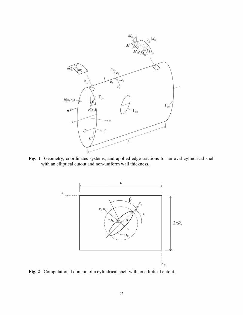
57

Fig. 1 Geometry, coordinates systems, and applied edge tractions for an oval cylindrical shell

with an elliptical cutout and non-uniform wall thickness.

Fig. 2 Computational domain of a cylindrical shell with an elliptical cutout.

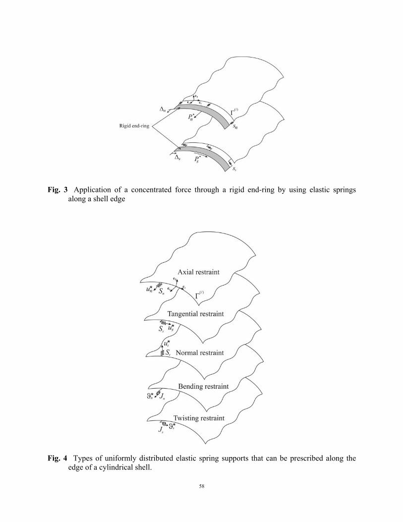
58

Fig. 3 Application of a concentrated force through a rigid end-ring by using elastic springs along a shell edge

Fig. 4 Types of uniformly distributed elastic spring supports that can be prescribed along the edge of a cylindrical shell.

59

Fig 5 The effect of varying shell radius on the tangential stress resultants around a circular

cutout in a quasi-isotropic circular cylindrical shell subjected to a uniform tension load.

Fig 6 The effect of varying circular-cutout radius on the tangential stress resultants around a

circular cutout in a quasi-isotropic circular cylindrical shell subjected to a uniform tension load.

60

Fig 7 The effect of varying elliptical-cutout aspect ratio on the tangential stress resultants

around a cutout in a quasi-isotropic cylindrical shell subjected to a uniform tension load.

Fig 8 The effect of varying elliptical-cutout orientation on the tangential stresses around the

cutout in a quasi-isotropic cylindrical shell subjected to a uniform tension load.

61

Fig 9 The effect of shell cross-section eccentricity on the stress-resultant concentration in an

oval quasiisotropic cylindrical shell with a circular cutout and subjected to a uniform tension load.

Fig 10 The effects of longitudinal ( 1 0ε ≠ and 2 0ε = ) and circumferential ( 1 0ε ≠ and 2 0ε = ) wall

thickness variations on the tangential stress-resultant concentration around a circular cutout in a quasi-isotropic circular cylindrical shell subjected to a uniform tension load.

62

Fig 11 The effect of varying shell radius on the tangential stresses around a circular cutout in a

quasi-isotropic circular cylindrical shell subjected to a uniform torsion load.

Fig 12 The effect of varying shell radius on the tangential stresses around a circular cutout in a

quasi-isotropic circular cylindrical shell subjected to a pure-bending load.

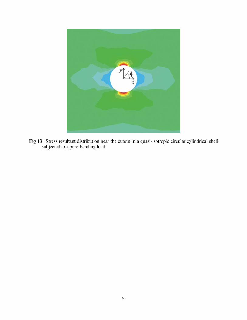
63

Fig 13 Stress resultant distribution near the cutout in a quasi-isotropic circular cylindrical shell

subjected to a pure-bending load.