stream function-vorticity driven cavity solution …frey/papers/navier-stokes/lid driven... ·...

Pergamon Computers & Fkids Vol. 26, No. 5, pp. 453468, 1997

0 1997 Elsevier Science Ltd. All rights reserved Printed in Great Britain

PII: SO0457930(97)00004-2 0045-7930/97 $17.00 + 0.00

STREAM FUNCTION-VORTICITY DRIVEN CAVITY SOLUTION USING p FINITE ELEMENTS

E. BARRAGY’ and G. F. CAREY2* ‘MS COl-02, Intel Corporation, 15201 N.W Greenbrier Pkwy, Beaverton, OR 97006, U.S.A.

‘TICAM, The University of Texas at Austin, Austin, TX 78712, U.S.A.

(Received 2 July 1996; in revised form 21 October 1996)

Ahstract~~alculations for the two-dimensional driven cavity incompressible flow problem are presented. A p-type Jinite element scheme for the fully coupled stream function-vorticity formulation of the Navier-Stokes equations is used. Graded meshes are used to resolve vortex flow features and minimize the impact of comer singularities. Incremental continuation in the Reynolds number allows solutions to be computed for Re = 12 500. A significant feature of the work is that new tertiary and quaternary corner vortex features are observed in the flow field. Comparisons are made with other solutions in the literature. 0 1997 Elsevier Science Ltd.

1. INTRODUCTION

This study presents results from a detailed set of calculations done for the steady 2D driven cavity problem. This problem has been studied extensively in the literature as a validation problem for 2D incompressible flow algorithms [l-20]. Results are available for finite element, finite difference/volume, exponential approximation and spectral methods. The present study combines several unique features not found elsewhere in the literature: A p-type finite element formulation combined with a strongly graded and refined element mesh provide for a highly accurate calculation. Use of parallel computing resources and incremental continuation allow a range of Reynolds numblers up to 12,500 to be explored on fine meshes [21]. The study begins with a summary of the stream function vorticity formulation. This is followed by examination of the detailed features in the flow field and comparisons to results in the literature. Values of local stream function extrema and separation points on the cavity walls are presented in tablular form to conclude the stu.dy. The results appear to be the most accurate available to date for this standard test problem. As this study deals with the steady problem directly, questions concerning loss of stability and time varying behavior are not addressed.

2. STREAM FUNCTION-VORTICITY FORMULATION

The stream function-vorticity formulation is a popular and well-established method for solving 2D incompressible viscous flow problems. The method is frequently applied to steady Stokes flow as a decoupled iterated system, since the problem then reverts to separate solutions of Poisson problems [22,23]. The present work utilizes a fully coupled stream function-vorticity approach in a weak variational formulation for the 2D steady Navier-Stokes equations. As in [24], the form of the vorticity boundary condition for the decoupled problem is readily deduced from this formulation. The resulting nonlinear system for the fully coupled problem is solved by Newton-Raphson iteration with incremental continuation in Reynolds number. The Jacobian systems are nonsymmetric and are solved approximately by a preconditioned biconjugate gradient (PBCG) scheme in an element-by-element (EBE) setting [25, 261.

*Department of Aerospace Engineering and Engineering Mechanics, CFD Laboratory, The University of Texas at Austin, Austin, TX 78712-1085, U.S.A.

453

454 E. Barragy and G. F. Carey

We wish to treat the coupled PDE system for stream function IJ and vorticity w corresponding to steady, 2D incompressible flow in domain R,

- V*o + Re(u.Vo) = f (1)

- v** - 0 = 0 (2)

where u = (u,v) is the velocity, with u = a$/ay, v = - 8$/8x, f is the body force and Re is the Reynolds number. Appropriate boundary conditions such as specified wall velocities (e.g. no slip) complete the mathematical statement of the problem.

The development of the coupled variational formulation is straightforward [24]. First choose test functions Y and q, which correspond to variations in IJ and o, respectively. Using these test functions in a weighted residual formulation of (l), (2) and applying the divergence theorem, the weak statement becomes: find II/ E H, w E G such that

s Vw.Vr dx dy + Re (u.Vw)r dx dy = n s n

s (Vt,bVq - oq) dx dy = n s

*q ds (3) as2 an

hold for admissible r, q. It is assumed that the boundary aR is divided into two parts, dR,, aR,. On aR,, let t,,Q = g be given as a Dirichlet condition and therefore r = 0 on Xl,. From (3) it is clear that unless o is also specified on aR, (resulting in q = 0 there), at,b/an must also be specified. This is just the tangential component of the velocity. On aR2, II/ is not specified. If r # 0, q # 0 one must specify both at//an and so/an. Alternatively, one could specify o and ac#n. Other combinations are possible and can be identified by assuming that r, q correspond to variations in $, o. As pointed out in [24,27], it is clear that the vorticity boundary conditions are given implicitly by equation (3) evaluated for nonvanishing test functions on the boundary. The approximate problem follows on introducing a finite element discretization and basis and replacing II/, o, r, q above by &, wh,

rh, qh.

3. DRIVEN CAVITY SOLUTION

This section presents results for the driven cavity problem on (0, 1) x (0, l), with unit lid velocity. The boundary conditions are + = 0 on aR and u, = 0 on an except at the lid where u, = 1. The discontinuity in u, at the corners can be treated in a variety of ways with differing success [28]. The issue is of greatest concern in primitive variable formulations since the nodal velocity enters directly as a solution variable. In the present formulation the weighted integral of u enters as implied by (3). This leads naturally to the following strategy when evaluating the boundary integrals: over the edge of each element the function u, is approximated with a piecewise linear interpolant. This interpolant has p + 1 evenly spaced nodes, where p is the degree of the polynomial in the finite element approximation for the element. The boundary integral is calculated via Gaussian quadrature and the piecewise linear interpolant of a, is used for the needed function evaluations. The value of u, at the nodes is specified as 1, except for those nodes that correspond to the corners of the cavity where the value is 0. For all of the results presented here a graded element mesh was used. The grading function x* = x + 1.99x(x - l/2), x I l/2 is applied to element corner coordinates. (Similar grading was applied for x 2 l/2 and for the y coordinates.) For the p-type elements used here, nodes within the element are evenly spaced, corresponding to a standard Lagrange basis. Several meshes are used, from p = 6, h = l/5 to p = 8, h = l/32. For the finest mesh, the grading function gives a smallest element size of 2.1 e-3 in the corner and a largest element size of 6.e-2, for a 3O:l ratio. The finest internode spacing is 2.6e-4. The present results were produced with an incremental continuation procedure using an increment of 500 in the Reynolds number and without body forces, f = 0 in (1). We remark that the choice of mesh grading was not extensively explored. The grading function given above was used with various quadratic scale factors, 1.90, 1.95, 1.99, 1.999. Based on oscillations in the vorticity, the values 1.90, 1.95 were found to have insufficient grading to resolve the boundary layer as Re increased. A value of 1.99

Stream function-vorticity driven cavity solution 455

iF

i- 100 400 1000 -

Table 1. Primary vortex stream function value

ti JI VI) ti ([71X extrap.

- 0.10005 - 0.10006 - 0.10330 - 0.10330 - 0.11389 - 0.11297 - 0.11399 - 0.11861 - 0.11603 - 0.11894

ti ([21)

-0.103423 - 0.113909 - 0.117929

was adequate for the range of Re considered. The reader is referred to [29,30] for more details on optimal grading and optimal h-p methods.

3.1. Comparison with results in literature

The driven cavity problem has been widely studied as an incompressible flow benchmark. One well-known stu.dy is that of [2], where a stream function-vorticity formulation is used with second-order accurate finite difference stencil in conjunction with second-order upwind treatment of the (nonlinsear) convective terms. Another well-known study is that of [7], which uses fourth-order di-fferencing with Richardson extrapolation in a continuation setting. As an initial comparison we would like to examine those results and compare them with the present p finite element formul;ation.

Table 1 shows the values of the stream function at the primary vortex center computed for various Reynolds numbers in the range 1 to 1000. For these results a graded 5 x 5 mesh of elements of degree p = 6 was used. The graded mesh corresponds to the tensor product of x and y coordinate values (0,0.08,O.32,0.68,0.92, 1). The agreement between the present results and the extrapolated values in [7] is remarkably good. The value of $,,,,, agrees to five digits for Re = 100 and shows differences of 1 .e-4 and 3.e-4 for Re = 400 and 1000, respectively. The method used in [7] is fourth-order accurate with Richardson extrapolation on typically a 120 x 120 grid. The results from [2] are from a 129 x 129 nodal mesh. Agreement with [2] is not as good at Re = 1000, but the method used there is only second-order accurate on a uniform grid and the lower mesh resolution is used. The table highlights several points. First, even for a very modest Reynolds number of 1000 there is substantial disparity in the results: - 0.1179 vs - 0.1189. Second, even for the fourth-order method there is a large difference between raw and extrapolated values: - 0.1160 vs - 0.1189. Finally, the high order p method with graded mesh does very well even though it has only 31 x 31 grid points.

This raises larger questions concerning solution accuracy. Table 2 presents a comparison with several sets of results in the literature for a larger range of Reynolds numbers Re = 1000, 5000, 7500 and 10,000, for the primary vortex strength. Also given is data for nominal mesh spacing, order of the method, and a flag for either uniform (U) or graded (G) meshes. In addition, a code

Rf2

h”,. s

h,. [71 Et

Al” [191 g

km (121 P

Ln 1161 L

*lmn [21 s

!L fl31 P

IL,,. fl51 g

$lm,n I171 g

*mm [141 s

loo0

Table 2. Primary vortex strength

5000 7500 10,000

.- 0.118930 257, 8, G - 0.11894 141, 4, u

- 0.119004 129, 8, U

- 0.118821 1024, 2, U - 0.1178 256, I, U

-0.117929 129, 2, U - 0.1163 257, 2, U - 0.1157 129, 2, U

- 0.11668 129, 2, U - 0.119 41. 2. G

- 0.122219 257, 8, G

- 0.122380 257, 8, G

- 0.122393 257, 8, G - 0.12292 180. 4, U

- 0.1214 256, 1, U

- 0.118966 257, 2, U - 0.1142 513, 2, u -0.1115 257, 2, U - 0.11621 129, 2, U - 0.122

41. 25 G

-0.1217 256, 1, U

- 0.119976 257, 2, U -0.1113

256, 2, U - 0.1052 257, 2, U

- 0.119731 257, 2, U - 0.1053 256, 2, U

- 0.11286 129, 2, U - 0.120 41. 2. G

rL.. fl81 g - 0.0977 - 0.0861 - 0.0873 51, 2 u 51, 2, u 51, 2. u

$.I. 1201 P -0.1178 - 0.1181 128, 2, U 256, 2, U


letter below each reference indicates the formulation: S-stream function vorticity, P-primitive variables, B-biharmonic, L-lattice Boltzman. Results for the present study are from a p = 8, h = l/32 graded mesh. Other results are as above from [2] and [7]; [15] where a second-order accurate method on a uniform mesh with Crank Nicholson time-stepping was used; [19] apply an 8th-order difference scheme on a uniform mesh with Runga Kutta time-stepping and also provide a mesh refinement study; [12] used a second-order accurate multigrid defect correction method on a particulary fine but uniform grid; [16] gives data for a uniform mesh lattice Boltzman method. Results in [13] apply a second-order method (upwind) on various uniform meshes. Additionally, there are results from [14, 17, 18, 201 for a variety of methods and resolutions; but where no data on primary vortex location was given. It should be acknowledged that in many of these references the authors do not claim particularly accurate solutions. Their focus may be on methodology and/or computational efficiency. However, it is still interesting to include them in the table for the sake of comparison.

Examining Table 2 at a Reynolds number of 1000, one immediately notices the wide range of values for the primary vortex strength. There are many aspects which could account for this wide range: mesh spacing and grading, accuracy/convergence rate of the method employed and issues such as upwinding, use of primitive variable or stream function-vorticity formulation, convergence criteria and arithmetic precision. For a Reynolds number of 1000 some comparisons can be made. The results of [ 181, while extending to very high Reynolds numbers, are for coarse uniform 50 x 50 meshes, and can be discounted. Similarly, in [14] a graded 40 x 40 mesh of bilinear elements is used, which is probably too coarse, although the results agree to three digits with those for more refined meshes. The results in [20] are for a second-order method on a uniform 128 x 128 mesh using primitive variables. The resolution here seems less than or comparable to other results. Similarly, in [17] the focus is on vorticity boundary conditions and a uniform 128 x 128 mesh is used. These results appear somewhat over-diffusive. Results for a Lattice Boltzman Method on a uniform 256 x 256 mesh are given in [16]. These results appear to fall in line with the present results and [2, 71. The results of [13] appear overly diffusive (an upwind method is used), while the results in [15] are for a second-order method, but with only 128 x 128 mesh points. Wright and Gaskell[12] give data for a uniform 1024 x 1024 mesh with second-order scheme and should be quite accurate. Nishida and Satofuka [19] use an 8th-order method on a uniform 128 x 128 mesh. Unfortunately their results and [12] do not extend to Re = 5000. Finally, Ghia et al. [2] use a second-order method with 128 x 128 mesh points for this value of Re. These results might then be considered somewhat under-resolved for Re = 1000. The results in [7] are extrapolated values for mesh sizes of 100 x 100 to 141 x 141, for a fourth-order method. Of these, comparing the vortex strength for the present results to those of [7, 12, 191 show all agree to within 6 = 0.0002, or almost four full digits.

At intermediate Reynolds numbers of 5000 and 7500, the present results agree well with those for the Lattice Boltzman method [16], but not as well with [2]. None of the other methods agree well with these values except for [14], although [20] and [2] agree well. Finally, at Re = 10 000, the agreement between the present results and [7] is quite good 6 = 0.0006, while comparing to [2] the difference in strength is larger 6 = 0.003. Overall, we believe the present results to be the most accurate to date, although the methods used may be less efficient than others.

Another aspect of Table 2 which is somewhat disturbing is the behavior of the primary vortex strength as the Reynolds number increases. For a sequence of three meshes (p = 8; h = l/8, h = l/l 6, h = l/32) the primary vortex achieved minimum stream function value at Reynolds numbers of approximately 7500,900O and 9500, respectively. Many of the results in the table show a trend of increasing stream function value as the Reynolds number increases. For example, [ 13, 15, 17, 181 all show evidence of this, which appears to be characteristic of an under- resolved solution or boundary layer. Even the results of [2] display this behavior to some degree.

In general, mesh grading and higher order methods appear to substantially improve the quality of the solution. For example, results in [14] at Re = 1000, 5000 compare well with only a 40 x 40 graded mesh. The present results and those of [19] and [7], all using high order methods, appear to be quite accurate. This is to be expected as resolving the boundary layer at higher Re is important to obtaining the correct solution. Finally, it would appear that the use of upwinding is quite detrimental, as seen by comparing the results of [13] with the present results or [2].


2 Fig. 1. Stream function and vorticity contours for Re = 5000.

CAF 2615-B


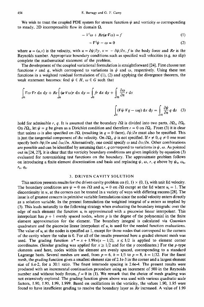
3 Fig. 2. Stream function and vorticity contours for Re = 7500.


3.2. Secondary jaw features

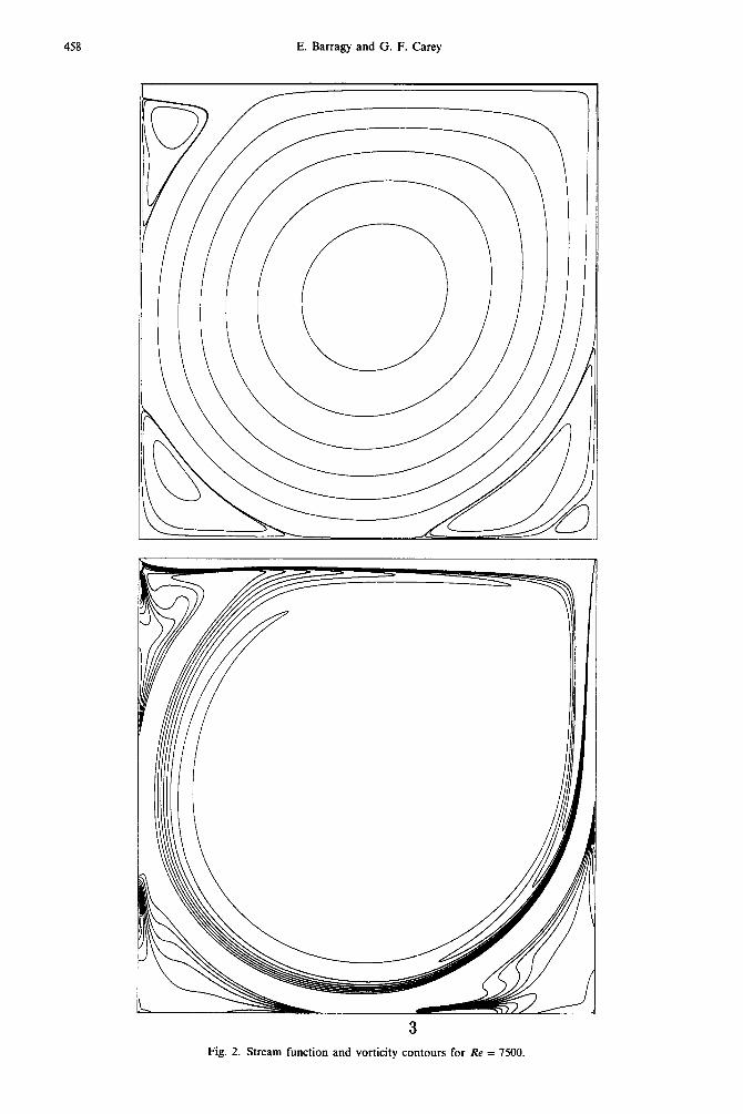
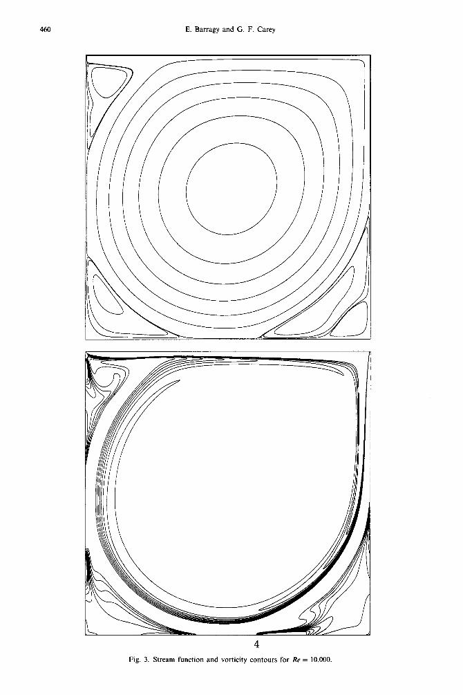
This section presents results on qualitative flow features found for the high resolution mesh h = l/32, p = 8. Figures 1 - 4 show computed streamlines for Reynolds numbers of 5000, 7500, 10,000 and 12,500. Contour values for the stream function plots are set to - 0.11, - 0.9, - 0.7, - 0.5, - 0.35 .- 0.1, - l.e-5, l.e-5, l.e-3, l.e-2. Contour values for the vorticity plots range are set to - 4, - 3., - 2, - 1, 0, 1,2, 3,4, 5. The figures show a smooth primary vortex accompanied by several secondary and tertiary vortices in the corn$rs. Specifically, the secondary and tertiary vortices can be identified in the lower right corner; while a secondary vortex can be identified in the lower left corner. The numerical results indicate that there are additional vortices in the lower right and lower left corners, although because of the contour intervals they do not show up in the figures. The upper left corner of the cavity presents an interesting flow feature at Re = 12,500: a secondary vortex which encloses a tertiary vortex. This tertiary vortex has not previously been identified although examination of results in [2] indicate its precursors in the Re = 10,000 solution. Figure 5, an under-resolved solution for h = l/16, p = 8 at Re = 16,000 clearly shows this vortex.

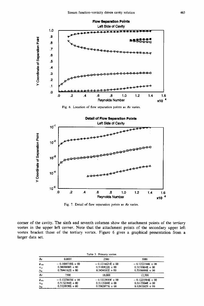
The location of separation points (as indicated by a sign change in vorticity on the wall) on the left side of the cavity are graphed as a function of Re in Fig. 6. The initial formation and subsequent growth of vortices on the left side of the cavity is clearly illustrated. The separation point (in the lower left corner) for the primary vortex is present for the Stokes problem and grows rapidly in size up to a Reynolds number of about 4000. Thereafter its location is roughly constant at y = 0.3. This separation streamline marks the boundary between the primary vortex and the secondary lower left corner vortex. A tertiary vortex is also evident in this figure, but does not begin to grow appreciably in size until a Reynolds number of 8000 is attained. The secondary vortex in the upper left corner is seen to appear between a Reynolds number of 1000 and 1500. It exhibits strong growth up to a Reynolds number of 10,000, whereupon an enclosed tertiary vortex appears (10,500 I Re I 11,000). This tertiary vortex has not previously been identified in numerical computations, although results in [2] show its precursors at Re = 10,000. Note that [9] indicates that a Hopf bifurcation occurs in this Re range for a regularized problem.

A detail of flow separation points on the left wall near the lower left corner is graphed in Fig. 7. The upper line plotted in this figure corresponds to the lower line in Fig. 6. Carefully counting the vortices implied by the flow separation points in these two figures indicates the detection of five nested vortices in this corner of the cavity. The first of the five is the primary cavity vortex, thus there are four vortices confined to this corner. The figure shows that the length scales of the recirculation zones vary by roughly one order of magnitude. For the graded mesh, the internode spacing is 2.6e-4 for the corner element, indicating that the fifth vortex appears at the grid frequency. This raises important questions about the reliability of the detection of the fifth vortex/fourth separation point. These results have been included for the sake of completeness.

3.3. Tabular results

Tables 3-6 give more extensive results for the graded mesh with p = 8, h = l/32. For example, Table 3 gives data for the primary vortex at the cavity center. The maximum stream function value and location are given for selected Reynolds numbers (Re). The next table gives the strengths and locations of secondary vortices in the lower right corner of the cavity. Tables 5 and 6 show similar data for the lower left and upper left corners respectively.

The data presented in Tables 3-6 are the raw output from the finite element post-processor. The data were produced by evaluating the finite element solution on a (4p + 1) x (4p + 1) set of points within each element. For each interior point, a test was applied to see if the value of the stream function at that point represented a local extremum with respect to its eight nearest neighbors. If so, the stream function value and location of the point were output. No filtering was done based on the strength of the vortex.

Table 7 shows the locations of separation points along the left edge of the cavity. This data is taken from the same mesh of solution values used for the data of Tables 3-6. The first four columns show the movement of separation points associated with vortices in the lower left corner: the fifth, quaternary, tertiary, secondary, and primary cavity vortices as the Reynolds number varies. The fifth and eighth columns show the attachment points of the secondary vortex in the upper left


Fig. 3. Stream function and vorticity contours for Re = 10,000.


6



E .Q ._

.8

i .7

g .8 l2 B

.5

10”

Flow Sqm-ation Points

Left Side of Cavity

.O .2 A .8 .8 1.0 1.2 1.4 1.8 Reynolds Number xl0 4

Fig. 6. Location of flow separation points as Re varies.

Detail of Flow Separation Points Left Side of Cavity

.O .2 .4 .8 .8 1.0 1.2 1.4 1.8 Reynolds Number x10

4

Fig. 7. Detail of flow separation points as Re varies.

corner of the cavity. The sixth and seventh columns show the attachment points of the tertiary vortex in the upper left corner. Note that the attachment points of the secondary upper left vortex bracket those of the tertiary vortex. Figure 6 gives a graphical presentation from a larger data set.

Table 3. Primary vortex

Re 0.0001 2500 5000 - IL nun -O.lOQO758E+OO -0.1214621E+00 -0.1222194E+OO &?r 0.5OO0OCOE+IXl 0.5188822E+OO 0.5151064E+ 00 Yk 0.76441628+00 0.5434181E +OO 0.5358696E+ 00

z- 7500 10,000 12,500

c - 0.12238038 + 00 -0.1223930E +OO -0.12235848+00 xx 0.51321848+00 0.5113304E+OO 0.5113304E + 00 Y!+X 0.5320950E +00 0.5302077E+OO 0.52832028+00


Table 4. Vortices in lower right corner

Re 0.0001 2500 5000

0.2227267&-05 0.9622189E+OO 0.3778106E-01 -0.61415878-10 0.99771448 + 00 0.2285573E-02 O.l534814E-I4 0.9998708E + 00 O.l292307E-03

0.2662249E-02 0.83423248+00 0.907512lE-01 -O.l226317E-06 0.9903702E +00 0.9321324E-02 0.3366884BII 0.9994164E + 00 0.5836428E-03 - 0,5945803E-15 0,9999354E+ 00 0.645819lE-04

0.30735158-02 0.8041016E + 00 0.72486528-01 -O.l427913E-05 0.97860178 +OO O.l881959E-01 0.38872898-10 0.9987615E +OO 0.11726798-02 -0,2272706E-14 0.9999354E +00 0.6458191E-04

Re 7500 10.000 12.500

0,3226968E-02 0,7900250E+ 00 0.6483485E-01 - 0.32790118-04 0.9517405E +00 0.42189WE-01 0.8899567E-09 0.99734218 +00 0.2657867E-02 - 0.2126772E-13 0.999806lE+OO O.l292307E-03

0.3191218E-02 0.7746636E +00 0.58780138-01 - O.l404461E-03 0.9351651E+00 0.67528338-01 0.39496268-08 0.9960358E+OO 0.3964201E-02 - 0,1044644E-12 0.9997413E+OO 0.2587290E-03

0.3099803E-02 0.7603326E +OO 0,5407320E-01 -0.2558322B03 0.92751358+ 00 0.81219448-01 0.77503508-08 0.9952875E+OO 0.4899706B02 -0,2077842E-12 0.99967648 +OO 0.25872908-03

RC?

Table 5. Vortices in lower left corner

0.0001 2500 5000

0.2227263E-05 0.3778106E-01 0.3778106E-01 -0.6141578E-IO 0.2285573&02 0.22855738-02 O.l534812E-14 0.12923078-03 O.l292307E-03

0.9310542E-03 0.8439557E-01 O.l109646E+ 00 - 0.28094618-07 0.6023922E-02 0.62113898-02 0.75958178-12 0.3884944E-03 0.38849448-03

0.13765048-02 0.72486528-01 0.13702978 +OO -0.66651278-07 0.78985718-02 0.7898571E-02 O.l814952E-11 0.5185267E-03 0.4534772E-03

7500

0.15364668-02 0.6416178E-01 0.15258898 +OO - 0.2043063E-06 O.l117058E-01 0.11786448-01 0.5591540E-II 0.6488255E-03 0.7140747E-03 -O.l141646E-I4 0.64581918-04 0.6458191B04

10,000

O.l619575E-02 0.5878013E-01 0.1622930E +OO -0.11334178-05 O.l733886E-01 0.2010944E-01 0.3074254E-IO 0.11069658-02 0.11069658-02 -0.22480008-14 0.645X1918-04 0.645819lB04

12,500

0.36677528-02 0.55418028-01 O.l680841E+OO -0.6787536E-05 0.2655169E-01 0.32X2161&01 0.1828415E-09 0.17670X0&02 O.l767080E-02 - 0,4384933E-I4 O.l292307E-03 0.645819lE-04

Re

Table 6. Vortices in upper left comer

0.0001 2500 5000

* ma” 0.3433099E-03 O.l447661E-02 Xlac 0.4329169E-01 0.63488808-01 YlW 0.8890354EfOO 0,9092488E+OO

Rf? 7500 10,000 125,000

ti "IA" 0.2134407B02 0.26304398-02 0,3006256E-02 &x 0.66854778-01 0.70224088-01 0.74074438-01 )‘I, 0.91163288 + 00 0.9108383E+OO 0.9100436E+00 ICI msx -0.17121338-05 Xlrr 0.7148820&02 "I_ 0.83075768+00

3.4. Accuracy

The question of the accuracy of the computed flow solutions presented in the previous section is an important one. Results in the literature rarely present systematic grid refinement studies due to the computational cost. Instead, comparisons to other results in the literature are made along


Rc

0. IOOOE-03 0.25OOE + 04 0.5000E + 04 0.75OOE + 04 O.IOOOE + 05 O.IZSOE + 05

Re

0. IOOOE-03 0.25OOE + 04 OSOOOE + 04 0.75OOE + 04 O.IOOOE + 05 0. I250E + 05

Table 7. Location of separation points on left side of cavity

#I #2 #3

0.334517E-03 OS56994E-02 0.9013698-03 O.l50456E-01

0.677357E-04 0. I 162858-02 0.1970858-01 0.879532E-04 0.1675008-02 0.297641E-01 O.l50193E-03 0.2725528-02 0.536455E-01 0.2559SOE-03 0.43 12238-02 0.83857lE-01

#5 #6 #7

0.7495658 + 00 0.6868328 + 00 0.6585088 + 00 0.640871 E + 00 0.628336E + 00 0.815670E + 00 0.8504808 + 00

#4

0.931569E-01 0.2334828 + 00 0.269 I84E + 00 0.285137E + 00 0.294439E + 00 0.300720E + 00

#8

0.934739E + 00 0.960474E + 00 0.969355E + 00 0.974214E + 00 0.977356E + 00

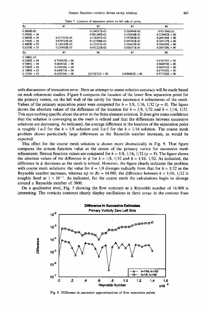
with discussions of truncation error. Here an attempt to assess solution accuracy will be made based on mesh refinement studies. Figure 8 compares the location of the lower flow separation point for the primary vortex, on the left wall of the cavity for three successive h refinements of the mesh. Values of the primary separation point were computed for h = l/8, l/16, l/32 (p = 8). The figure shows the absolute values of the difference of the location for h = l/S, l/32 and h = l/16, l/32. This says nothing specific about the error in the finite element solution. It does give some confidence that the solution is converging as the mesh is refined and that the differences between successive solutions are decreasing. As indicated, the average difference in the location of the separation point is roughly 1 .e-3 for the h = l/S solution and 3.e-5 for the h = l/l 6 solution. The coarse mesh problem shows particularly large differences as the Reynolds number increases, as would be expected.

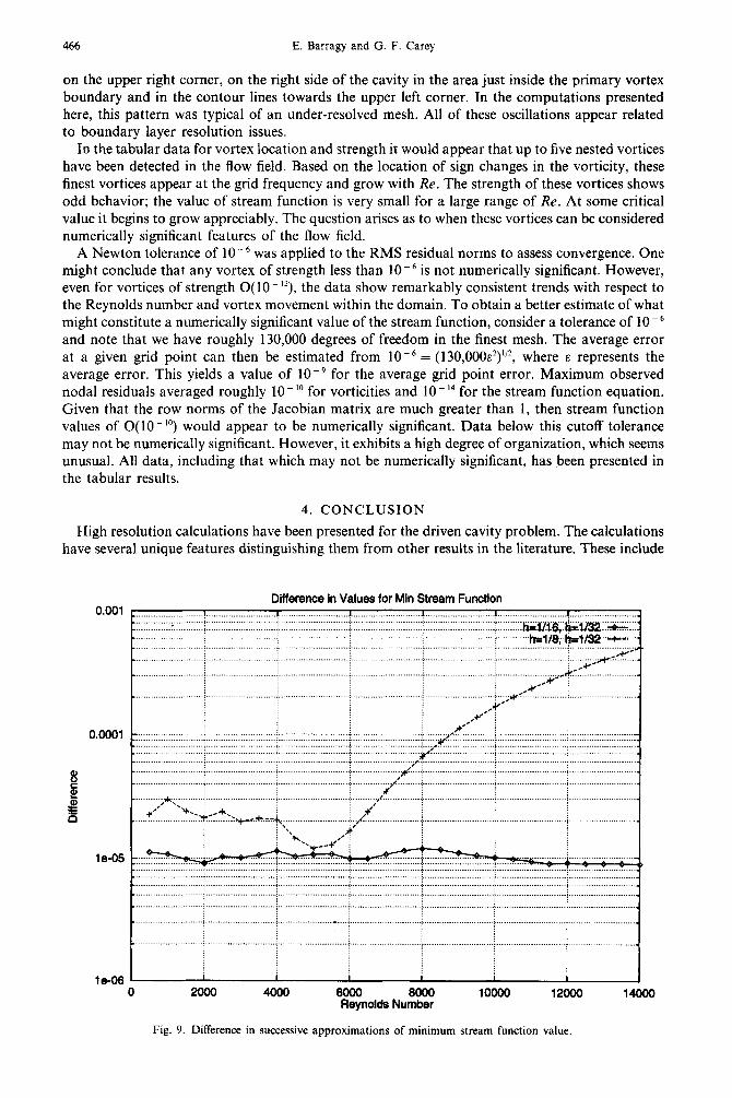
This effect for the coarse mesh solution is shown more dramatically in Fig. 9. That figure compares the st.ream function value at the center of the primary vortex for successive mesh refinements. Stream function values are compared for h = l/S, l/16, l/32 (p = 8). The figure shows the absolute values of the difference in tj for h = l/S, l/32 and h = l/16, l/32. As indicated, the difference in $ decreases as the mesh is refined. However, the figure clearly indicates the problem with coarse mesh solutions: the value for h = l/8 diverges radically from that for h = l/32 as the Reynolds number increases, whereas up to Re = 14 000, the difference between h = l/16, l/32 is roughly fixed at 1 x 10 - 5. As indicated, for the coarse mesh the calculations begin to diverge around a Reynolds number of 5000.

On a qualitative level, Fig. 5 showing the flow contours at a Reynolds number of 16 000 is interesting. The ,vorticity contours clearly display oscillations in three areas: in the contour lines

1o-2

1o-3

!I lo4

f

B 10”

los

lo-’ .u

Difference in Succesive Estimates Primary Vorticity Zero Left Side

+ h=lIiB, h-l/32 -6- h=1/8. hd32

.2 A .6 .8 1.0 1.2 1.4 1.6 Reynolds Number x10 4

Fig. 8. Difference in successive approximations of flow separation points.


on the upper right corner, on the right side of the cavity in the area just inside the primary vortex boundary and in the contour lines towards the upper left corner. In the computations presented here, this pattern was typical of an under-resolved mesh. All of these oscillations appear related to boundary layer resolution issues.

In the tabular data for vortex location and strength it would appear that up to five nested vortices have been detected in the flow field. Based on the location of sign changes in the vorticity, these finest vortices appear at the grid frequency and grow with Re. The strength of these vortices shows odd behavior; the value of stream function is very small for a large range of Re. At some critical value it begins to grow appreciably. The question arises as to when these vortices can be considered numerically significant features of the flow field.

A Newton tolerance of 10 -6 was applied to the RMS residual norms to assess convergence. One might conclude that any vortex of strength less than 10m6 is not numerically significant. However, even for vortices of strength 0( 10 - I’), the data show remarkably consistent trends with respect to the Reynolds number and vortex movement within the domain. To obtain a better estimate of what might constitute a numerically significant value of the stream function, consider a tolerance of 10m6 and note that we have roughly 130,000 degrees of freedom in the finest mesh. The average error at a given grid point can then be estimated from 10m6 = (130,000~*)“*, where E represents the average error. This yields a value of 10m9 for the average grid point error. Maximum observed nodal residuals averaged roughly 10 - ‘O for vorticities and 10 -I4 for the stream function equation. Given that the row norms of the Jacobian matrix are much greater than 1, then stream function values of O(l0 -I”) would appear to be numerically significant. Data below this cutoff tolerance may not be numerically significant. However, it exhibits a high degree of organization, which seems unusual. All data, including that which may not be numerically significant, has been presented in the tabular results.

4. CONCLUSION

High resolution calculations have been presented for the driven cavity problem. The calculations have several unique features distinguishing them from other results in the literature. These include

Difference in Values for Min Stream Function 0.001 t . __...._._..___............: 4..

: . . . . . . . . . . . . . . . . . . . . . . . . . . . . . . . . . . . . . . . . . . . . . . . . . . . . . . . . . . . . . . . . . . . . . . . i

/ (............................ i . . . . . . . . . . . . . . . . . . . . . . . . . . . . . . . . . . . . . . . . . . . . . . . . . . . . . . . . . . . h&j&:&I/~~::&G:::: ______..___.._._..__........ j . . . . . . . . ..__._._...__..._..~ !_ f . . . . . . . . . . . . .._...._._......~ h_q./*..$+3t&. _ _____..__..............: i.. . . . . . . . . . . . . . . . . . . . . . . . . . . I . . . . . . . . . . . . . . . . . . . . . . . . . . . . . . . . . . . . . . . . . .. .T: .......! ....: ............ ?I:,. _.____..___.......,.........; . . . . . . .._........_..........~ __.........................; . . . . . . . . . .._.................~ . . .._.............. ~...................__....... j..._+&....

o.jcK), k :::::::::::::::::: ::::::: j :::::::::::::::::::::::::::: ;:_: :::::::::::::::: ::::::::: j :::::::::::::: :::::::::::::: .j ::::::__ &:. ........... . ............................ .......................... j ........................... i ............................ i__ j .......................... ............................. i...,Y’:::::::::::::::::::I::::::::::::::::::::::::::::;:::::::::::::::::::::::::: : > A _____.____.______.......... j . . . . . . . . . . . . . . . . . .._......... . . . . . . . . . . . . . . . . . . . . . . . . . . . . . _..______.._.............. +$i ..__...____._.._......... j . . . . . . .._.._____..___........ . . . . ..___________________ < __._________ ._.._.__..____ ____..___..___...____ i .______.____..______........ <__ )___________________......... [ ._......................._.

t .-..........,....-.-..-.-.~....---.-------..-..........~..-.............-.--..---...~.................~....--..-~----..-.-............. .-...~-.-.....-.-............-...~-.-..- ....-.-.....--._-..

j i. i ,*i...;. , i ......................._....; __,. .............__.._..

le-06 1 I I I 1 I I 1 0 2ooo 4000 6ooo Nu12 10000 12000 14000

Reynolds

Fig. 9. Difference in successive approximations of minimum stream function value.


the use of a high ,u finite element approximation (p = 8) and a graded element mesh (30: 1) element size ratio. These factors significantly improve solution accuracy and help to minimize the impact of corner singularities. Several unique flow features have been observed which are not reported elsewhere. This includes tertiary and quaternary corner vortices and an enclosed tertiary corner vortex in the upper (upstream) corner. This vortex is attached to the cavity wall and enclosed by the secondary corner vortex. The present results include comparison to other results in the literature (to assess accuracy) as well as grid refinement studies of the location of flow separation points and the stream function value for the primary vortex to assess solution accuracy. Detailed comparisons are given as the Reynolds number varies.

AcknoM,ledgemenrs--This research has been supported by the Department of Energy CLS fellowship program and by NASA.

1.

2.

3.

4.

5.

6.

7.

8.

9.

10.

Il.

12.

13.

14.

15.

16.

17.

18.

19.

20.

21.

22. 23. 24.

25.

26.

27.

28.

REFERENCES

Cortes, A. B. and Miller, J. D., Numerical experiments with the lid driven cavity flow problem. Compurers & Fluids, 1994, 23, 1005-1027. Ghia, U., Ghia, ;K. and Shin, C., High Re solutions for incompressible flow using the Navier-Stokes equations and a multigrid method. Journal of Computarional Physics, 1982, 48, 387411. Goodrich, J., Gustafson, K. and Halasi, K., Hopf bifurcation in the driven cavity. Journal of Computational Physics, 1990, 90, 219-261. Gustafson, K. and Halasi, K., Cavity flow dynamics at higher Reynolds numbers and higher aspect ratios. Journal of Computational Physics, 1987, 70, 271-283. Huser, A. and Biringen, S., Calculation of two dimensional shear driven cavity flows at high Reynolds numbers. International Journal of Numerical Methods in Engineering, 1992, 14, 1087-I 109. Kim, J. and Moin, P., Application of a fractional step method to incompressible Navier-Stokes equations. Journal of Computational Physics, 1985, 59, 308-323. Schreiber, R. and Keller, H. B., Driven cavity flows by efficient numerical techniques. Journal of Computational Physics, 1983, 49, 31&333. Schreiber, R. and Keller, H. B., Spurious solutions in driven cavity calculations. Journal of Computational Physics, 1983, 49, 165-172. Shen, J., Hopf bifurcation in the unsteady regularized driven cavity flow. Journal of Computational Physics, 1991, 95, 228-245. Shen, C. Y. and Reed, H. L., Application of a solution adaptive method to fluid flow: line and arclength approach. Computers & Fluids, 1994, 23, 373-395. Sohn, J., Evaluation of FIDAP on some classical laminar and turbulent benchmarks. Infernational Journal of Numerical Methods for Fluids, 1988, 8, 1469-14907. Wright, N. G. and Gaskell, P. H., An efficient multigrid approach to solving highly recirculating flows. Computers & Fluids, 1995, 24, 63-79. Bruneau, C. H. and Jouron, C., An efficient scheme for solving steady incompressible Navier Stokes equations. Journal of Computational Physics, 1990, 89, 389413. Comini, G., Ma.nzan, M. and Nonino, C., Finite element solution of the streamfunction vorticity equations for incompressible two dimensional flows. International Journal of Numerical Methods for Fluids, 1994, 19, 513-525. Goyon, O., High Reynolds number solutions of Navier Stokes equations using incremental unknowns. Computer Methods in Applred Mechanics and Engineering, 1996, 130, 319-335. Hou, S., Zou, Q,, Chen, S., Doolen, G. and Cogley, A., Simulation of cavity flow by the lattice Boltzman method. Journal of Computational Physics, 1995, 118, 329-347. Huang, H. and Seymour, B., The no slip boundary condition in finite difference approximations. Infernational Journal of Numerical Methods for Fluids, 1996. 22, 713-729. Nallasamy, M. and Prasad, K., On cavity flow at high Reynolds numbers. Journal of Fluid Mechanics, 1977, 79, 391414. Nishida, H. and Satofuka, N., Higher order solutions of square driven cavity flow using a variable order multigrid method. International Journal of Numerical Methods in Engineering, 1992, 34, 6376531. Thompson, M. C. and Ferziger, J. H., An adaptive multigrid technique for the incompressible Navier Stokes equations. Journal of Computational Physics, 1989, 82, 94121. Barragy, E., Carey, G. F. and Van de Geijn, R., Parallel performance and scalability for block preconditioned finite element (p) solution of viscous flow. International Journal of Numerical Methods in Engineering, 1995, 38, 1535-1554. Carey, G. F. and Oden, J. T., Finite Elements: Fluid Mechanics. Prentice Hall, Englewood Cliffs, NJ, 1986. Roache, P. J., C~smputational Fluid Dynamics. Hermosa, Albuquerque, NM, 1972. Campion-Renson, A. and Crochet, M. J., On the stream function-vorticity finite element solutions of Navier-Stokes equations. International Journal of Numerical Methods in Engineering, 1978, 12, 1809-1818. Hughes, T. J. R., Levit, 1. and Winget, J., Element-by-element solution algorithm for problems of structural and solid mechanics. Computer Methods in Applied Mechanics and Engineering, 1983, 36, 241-254. Barragy, L. and Carey, G. F., Stream function vorticity solution using high degree finite elements and element by element techniques. Communications in Numerical Methods in Engineering, 1993, 9, 387-395. Dennis, S. C. R.. and Quartapelle, L., Some uses of Green’s theorem in solving the Navier-Stokes equations. International Journal of Numerical Methods for Fluids, 1989, 9, 871-890. McLay, R. and Carey, G. F., Local pressure oscillations and boundary treatment. International Journal of Numerical Methods for FlubIs, 1986, 6, 155-172.


29. Babuska, I. and Guo, B., The h, p. h-p version of FEM for I-d problem: I p error analysis, 11 h, h-p error analysis, III adaptive h-p. Numerical Mathematics, 1986, 49, 577-683.

30. Oden, J. T., Wu, W. and Legat, V., An hp adaptive strategy for finite element approximations of the Navier Stokes equations. International Journal of Numerical Methoris ,for Fluids, 1995, 20, 83 I-851.

stream function-vorticity driven cavity solution …frey/papers/navier-stokes/lid driven... ·...

Documents