International Journal of Computer Systems Science & Engineering, v. 13, no. 1, January 1998, pp. 5-16

1

Strategies for the Implementation of Interconnection Network Simulators on Parallel Computers*

Michael Jurczyk Thomas Schwederski

Department of Computer Science Institute for Microelectronics Stuttgart and Computer Engineering Allmandring 30a,University of Missouri at Columbia D-70569 Stuttgart, Germany121 Engineering Building WestColumbia, Missouri 65211, USATel.: (+1) 573-884-8869 Tel.: (+49) 711-685-5924Fax: (+1) 573-882-8318 Fax: (+49) 711-685-5930mjurczyk@cecs.missouri.edu schwederski@mikro.uni-stuttgart.de

Howard Jay Siegel Seth Abraham

Parallel Processing Laboratory Intel CorporationSchool of Electrical and CH11-102 Computer Engineering, 6505 W Chandler BlvdPurdue University Chandler, AZ 85226-3699, USAWest Lafayette, IN 47907-1285, USATel.: (+1) 765-494-3444 Tel.: (+1) 602-552-3027Fax: (+1) 765-494-2706 Fax: (+1) 602-554-7774hj@purdue.edu seth_abraham@ccm.ch.intel.com

Richard Martin Born

Symbios Logic, Inc.2001 Danfield CourtFort Collins, CO 80525-2998, USATel.: (+1) 970-223-5100x9701Fax: (+1) 970-226-9686rick.born@symbios.com

2

AbstractMethods for simulating multistage interconnection networks using massively parallel

SIMD computers are presented. Aspects of parallel simulation of interconnection

networks are discussed and different strategies of mapping the architecture of the network

to be simulated onto the parallel machine are studied and compared. To apply these

methods to a wide variety of network topologies, the discussions are based on general

interconnection network and switch box models. As case studies, two strategies for

mapping synchronous multistage cube networks on the MasPar MP-1 SIMD machine are

explored and their implementations are compared. The methods result in a simulator

implementation with which 109 data packets can be simulated in 40 minutes on the MasPar

system.

Keywords: mapping strategies, multistage interconnection networks, parallel

simulation, parallel processing, SIMD machine, time-driven simulation

*This research was supported in part by the German Science Foundation DFG scholarship

program GK-PVS, and by NRaD under contract number N68786-91-D-1799. Some of

the equipment used was provided by NSF under grant CDA-9015696.

Acknowledgments: A preliminary version of portions of this material was presented at the

1994 International Conference on Parallel Processing. The authors thank Janet M. Siegel

for her comments.

3

1. Introduction

In many parallel processing systems, multistage interconnection networks are used to

interconnect the processors, or to connect the processors with memory modules, e.g.,

ASPRO, BBN Butterfly, Cedar, NEC Cenju-3, IBM RP3, IBM SP-2, PASM, STARAN,

Ultracomputer [2, 15, 21, 22, 23, 24, 25, 26]. Many implementation parameters, such as

switch box size and buffer organization, have a major influence on network performance

[17]. These parameters must be evaluated by simulation and/or analysis prior to network

implementation to achieve an effective system.

To reduce the very long execution times of network simulations, the use of a massively

parallel system is studied here. Various parallel network simulators based on the discrete

event simulation technique have been implemented on MIMD and SIMD machines, e.g.,

[1, 7]. For certain network classes, e.g., synchronous networks, the time-driven simulation

technique is often superior to the event-driven simulation method. Thus, in this paper,

mapping strategies for time-driven simulators on SIMD computers are discussed and

compared to obtain an efficient simulator. To make those methods applicable to a wide

variety of network topologies, the study is based on a general interconnection network

model.

In the next section, network and switch box models are presented. These models are

used in Section 3 to discuss aspects of parallel simulation and to study and compare

different mapping strategies. A simulator implemented on the MasPar MP-1 and its

performance are overviewed in Section 4.

2. General Network and Switch Box Models

To make the discussions on simulator optimization applicable to a wide variety of

network topologies, the optimization strategies presented here are based on a general

network model. This model of unidirectional multistage interconnection networks is

depicted in Figure 1. A network connecting N sources with N destinations consists of s

stages (s ≥ 1). Each stage i consists of b switch box entities that communicate with the

successor stage via a stage interconnection unit. This unit represents static

4

interconnection patterns between two adjacent stages. The boxes in a stage may be

controlled by a stage control unit, and/or by boxes of adjacent stages (for inter-stage data

flow control). The boxes in the first and the last stage may additionally be controlled by

the sources and destinations, respectively. The stage control entity, which is controlled by

a network control entity, models the stage settings as required in permutation networks,

for example. In self-routing networks, the stage and the network control units can be

omitted.

A general switch box model is depicted in Figure 2. A box provides pi input ports and

po output ports. These ports can forward data and control signals. Data at the input ports

are buffered in qi input queues, which have a queue length of li each. The data is then

transferred to qo output queues with queue length lo each via a switch routing unit. The

data leaves the box at the output ports. The queue model also determines which data type

is to be transferred through the network, e.g., data bytes or data packets. Each queue

array is controlled by a queue control unit. This control unit determines the queueing

policy, e.g., a FIFO queue policy. The queue control unit may be controlled by a box

control unit. This box control unit may also interact with other switch boxes via the input

and output ports to model, for example, flow control strategies within a network.

This general box model can be used to model a broad variety of switch boxes. For

example, an output buffered switch box with input latches as shown in Figure 3(a) [5, 14]

can be modeled by choosing the input queue length qi to be one and specifying a crossbar

switch for the switch routing unit. If the output queues are discarded from the model in

Figure 2, an input buffered switch box (Figure 3b) [8, 18] can be modeled.

Now consider a central memory buffering switch as shown in Figure 3(c) [20]. Without

a buffer allocation constraint, incoming packets are stored in the central memory as long

as the memory with size M is not full. With buffer allocation limitation, incoming

packets are stored in the central memory as long as either the memory is not full, or the

number of packets stored in the memory that are destined to a particular output port does

not exceed a limit LI. This mechanism ensures that during asymmetrical data traffic, data

destined to a particular output port cannot occupy all buffers in the central memory. One

way to represent this switch using the structure in Figure 2 is to omit the input queues and

5

set the length of each output queue to LI. Then the box control unit of a central memory

switch refuses to accept incoming packets if the occupied memory exceeds the size M or if

the length of the output queue to which a packet is destined exceeds the limit LI.

The above discussion demonstrates that the network and the box models can be used to

represent a broad variety of interconnection networks. These models are therefore used in

the following discussion on parallel simulation of interconnection networks.

3. Parallel Simulation Aspects of Interconnection Networks

3.1 Time- Versus Event-Driven Simulation Strategies

The two major simulation methods are event-driven and time-driven [30]. The choice

of style has a major influence on simulator performance and depends on the events to be

simulated. If the density of event occurrence is low, the event-driven simulation should be

used. If a high probability of simultaneous events is expected, the choice of the simulation

style is dependent upon the event characteristics. Synchronous events can be simulated

efficiently with the time-driven style, while the event-driven style should be used with

asynchronous events. The simulation style also affects the best choice of the parallel

computer architecture to be used. MIMD machines with their asynchronous processors

are well suited to support the event-driven simulation style. Because in SIMD machines all

processors operate synchronously, a time-driven simulation can exploit the machine power

efficiently by using this implicit synchronization. Ayani and Berkman, on the other hand,

have shown that although the processors operate synchronously, it is still possible to

implement an event-driven simulator on a SIMD machine [1].

When simulating interconnection networks, the characteristic of the data traffic must be

considered to obtain an efficient simulator. In most cases, the traffic patterns of interest

are either uniform traffic or, more often, a superposition of various traffic types, such as

burst/silence traffic with uniform background traffic, or hot-spot traffic with uniform

background traffic, e.g., [29]. Thus, traffic patterns with lower densities of event

occurrence are frequently mixed with traffic that exhibits high event densities. This results

in continuous network activities that can be simulated efficiently using the time-driven

6

simulation style, assuming synchronous events. In the following discussion, the

effectiveness of the time-driven simulation approach implemented on a SIMD machine will

be demonstrated.

3.2 Mapping Strategies

Mapping strategies of synchronous networks on SIMD machines that use the

time-driven simulation style are considered in this section. A distributed memory SIMD

machine architecture with NS PEs (processing elements that are processor/memory pairs),

as depicted in Figure 4, is assumed. The PEs communicate via an interconnection network

and receive instructions from a common control unit.

Depending on the model used, a consequence of communication in a SIMD machine is

the loss of data if two or more PEs try to send data simultaneously to one variable in a

particular PE [12]. In this case, memory locations are overwritten during the data transfer,

and the destination PE only receives the last data item that was sent. This data loss can be

avoided by either serializing the data transfers, or by appropriate program sequencing. The

transfer serialization method will be shown in the link mapping strategy in Section 3.3.3,

while program sequencing and serialization is used in the box mapping as discussed in

Section 3.3.4.

The implementation of a network simulator on a large-scale SIMD machine gives the

programmer multiple choices for how to map the network structure onto the machine. An

efficient mapping and, accordingly, improved program performance, depend on the SIMD

machine architecture. To study the impact of the architecture on the efficiency of different

mapping strategies, the following measures are considered:

• number of PEs, i.e., NS,

• PE speed and complexity,

• amount of memory per PE,

• inter-PE communication topology and speed.

The number of PEs and the available memory space per PE differ significantly between

machines (e.g., 64K PEs with 8Kbyte RAM each for one configuration of the CM-2 [28],

7

16K PEs with 16Kbyte RAM each for one configuration of the MasPar MP-1 [3]). Also,

the topology and speed of the network connecting the PEs differ. Some machines, like the

MPP [2], only provide a mesh network for communication, while other machines, like the

MasPar MP-1 [3], provide a fast mesh network and a slower multistage router network

for global communication.

A major distinction between the various mapping strategies is the mapping

granularity, which is defined here as the degree of parallelism inherent in the mapping.

Consider the case of mapping multistage interconnection networks on a parallel computer.

Then, fine-granularity mapping is the mapping of an individual network link with the

related input and output buffers onto one PE (link mapping, as shown in Figure 5a).

Medium granularity is the mapping of a single switch box onto one PE (box mapping,

Figure 5b), while the mapping of multiple boxes onto one PE is of coarse granularity

(multibox mapping, Figure 5c). The trade-offs among these mapping strategies will now

be discussed.

It is assumed that in many cases the simulator performance is improved by executing

multiple simulations of the same network in parallel and averaging the results, thereby

exploiting the available machine power. To prevent conflicts among these sub-simulations,

each sub-simulation uses different PEs. Therefore, if the mapping of one network onto a

target machine needs P PEs, while the target machine provides NS PEs, it is assumed that

NS/P network sub-simulators are mapped onto the target machine and are executed in

parallel.

Mapping granularity. The finer the mapping granularity, the greater the number of PEs

that are used per network sub-simulator. This causes a relatively low number of parallel

sub-simulators in the link mapping. With coarser mappings, fewer PEs are used per

sub-simulator, and thus more execution time is needed for a simulation run. However,

more concurrent sub-simulators can be executed than with a finer mapping. Therefore,

with a fine granularity mapping, few but fast parallel sub-simulators can be implemented,

while with medium and coarse granularity, more but slower sub-simulators are obtained.

Because the actual performance of the different mappings is implementation-dependent,

actual execution times must be measured to determine the best mapping. This will be

8

discussed in Section 3.3.5.

Communication overhead. The inter-PE communication network(s) of the target

machine may influence the choice of the mapping strategy to be used if the transfer times

of the available inter-PE communication network(s) are distance and traffic dependent. If a

local network (e.g., a mesh) is used, the transfer time is dependent on the communication

distance. The more PEs used for one sub-simulator, the longer the average communication

distance between these PEs. In this case, a coarse granularity mapping that uses few PEs

with a low communication distance is preferable from the overhead of communication

point of view. If a multistage global network is available, the communication distance is

the same for all source/destination pairs of PEs. Thus, it does not effect the mapping

choice.

Memory requirements. Because in box and multibox mappings, all buffer queues of one

or multiple switch boxes reside in each PE, compared to only two queues in link mapping,

box and multibox mappings require more memory per PE than link mapping. This can be a

major drawback of the box and multibox mappings, especially in SIMD machines,

because the memory space per PE is typically limited. Consider, for example, the data type

to be transferred through the simulated network, which influences the queue model of the

switch box depicted in Figure 2. If data types are modeled on the byte-level and longer

data packets are to be simulated (e.g., Asynchronous Transfer Mode switching (ATM) [9]

with 53 byte packets), the required memory might exceed the available memory per PE

with box and multibox mapping, depending on the switch box size and the buffer length.

Switch box functions. If network functions that operate on a switch box rather than on

single links and/or buffers (e.g., memory length calculation with central memory buffering)

must be mapped, a medium to coarse granularity will give better performance. In these

mappings, information and data of complete switch boxes reside in a single PE, so that

box operations can be performed efficiently. In link mapping, however, information about

the switch box status resides in multiple PEs, so that inter-PE communication is necessary

to perform a switch box operation. This issue will be further discussed in Section 3.3.5,

where the effect of central memory buffering on the performance of link and box mapping

implementations is examined.

9

The trade-offs discussed above are summarized in Figure 6. Two mappings (link and

box mapping) of a multistage cube network onto the PEs of the MasPar MP-1 target

machine are examined and compared in case studies in the next sections.

3.3 Case Studies: Two Strategies for Mapping Synchronous Multistage Cube Networks on the MasPar MP-1 SIMD Machine

3.3.1 Overview of Multistage Cube Networks

The networks considered in the following are synchronous, store-and-forward packet

switching multistage cube networks [21, 22, 23], connecting N = 2n inputs with N outputs.

Multistage cube networks are representatives of a family of topologies that includes the

omega [16], indirect binary n-cube [19], delta [6], baseline [31], butterfly [4], and

multistage shuffle-exchange networks [27]. They can be constructed by using BxB

crossbars so that the network has s = logB N stages of N/B switch boxes each. It is

assumed that N is a multiple of B. A multistage cube network with N = 16 and B = 4 is

shown in Figure 7. Considering the general network model discussed in Section 2, the

multistage cube network model consists of s stages with N/B switch boxes per stage.

Because a self-routing network is assumed, the stage control and the network control

units in the network model are omitted. This model is used in the following sections to

discuss different simulation strategies.

3.3.2 Overview of the MasPar MP-1 Machine Architecture

The MasPar MP-1 parallel computer [3] is a SIMD machine with up to 16K PEs. Each

PE is a 4-bit load/store arithmetic processor with dedicated register space and 16 Kbytes

of RAM in the configuration under consideration. The PEs are arranged in a

two-dimensional matrix in which each non-overlapping square matrix of 16 PEs forms a

cluster. The MP-1 has two different interconnection networks for inter-PE

communication, which are shown in Figure 8 [3]. The eight-nearest-neighbor X-Net

provides fast communication between adjacent PEs, while a slower three-stage global

10

router provides communication between arbitrary PEs.

3.3.3 Link-Mapping Strategy

In link mapping, a BxB switch box is mapped onto 2*B PEs, as shown in Figure 9.

Each PE controls one output buffer of stagei and the corresponding input buffer of

stagei+1. Thus, inter-stage and intra-stage transfers (which consist of data movements

within and between PEs, respectively), queue handling, and statistical operations are

required.

Due to the mapping, an inter-stage transfer can be performed in a single step, in all PEs

simultaneously. To transfer a packet through a switch box (i.e., from input queue to

output queue), inter-PE communication must be used. To avoid the loss of data as a

consequence of the SIMD inter-PE communication, as discussed in Section 3.2, the

intra-stage data transfers must be serialized, which will now be discussed.

Consider, for example, a 2x2 switch box of stagej in a multistage cube network as

depicted in Figure 10. First, assume that the head packet of the upper input queue qui0 is

destined to the upper switch box output queue quo0, while the head packet of the lower

input queue qui1 is destined to the lower switch box output queue quo1. Thus, at this

intra-stage transfer simulation cycle, data must be transferred from PEi to PEk, and from

PEj to PEm. Because only one data item is destined to each destination PE, these data

transfers can be executed in parallel in a single step.

Now assume that the head packets of both input queues (qui0 and qui1) are destined to

the upper switch box output queue quo0, as depicted in Figure 10. For this intra-stage

transfer, two data items, originating from PEi and PEj, must be sent to PEk. If these

transfers were executed in parallel in a single step, PEk would receive one data item only,

while the other one would be lost due to the SIMD inter-PE communication, as discussed

in Section 3.2. Thus, this data transfer must be serialized into two steps to ensure correct

data transmission.

In general, because the packet destination addresses are dependent on simulation

parameters that may be generated at execution time and are not known a priori, each

11

intra-stage data transfer must be serialized to prevent data loss. During each intra-stage

data transfer, up to B packets at the heads of the switch box input queues can be destined

to the same particular output queue, and thus must be routed to the output queue in one

particular PE. To avoid data loss, these B transfers therefore must be performed serially in

B steps.

Assume the structure of a multistage cube network as shown in Figure 11. This

serialization can be done using the global router as follows, given each PE knows the

relative box number, from 0 to (N/B)-1, of the input queue it is simulating within a

network stage. First, all PEs whose relative box number is (0 mod B) transmit data and the

receiving PEs store the data appropriately. Then, all PEs whose relative box number is (1

mod B) transmit data, etc. This serializes the B steps correctly.

Each PE must know the number of the PE simulating the output queue to which its

input queue data is destined. This assignment of PEs to queues can be done in different

ways (an example for central memory buffering is given below) and the potential

destination PE addresses (for output queues) are stored in each PE (simulating the

corresponding input queues).

During a simulation cycle, data packets must be generated at the network inputs in

accordance with the selected traffic model and load. Then, a data transfer between the

network stages must be performed. This operation includes the actual transfer and the

statistics calculation. Finally, a data transfer through the switch boxes must be performed,

which also includes the actual transfer and statistics calculation. Assume that TPGEN is the

execution time needed to generate data packets during one simulation cycle, and that

TSTAGE is the time needed to execute all operations associated with an inter-stage data

transfer. Furthermore, TBOX is assumed to be the time required to execute all operations

associated with a transfer through a switch box during a simulation cycle. Because of the

necessary communication serialization, one simulation cycle requires the execution time:

TCYC,link = 1 * TPGEN + 1 * TSTAGE + B * TBOX . (1)

With central memory buffering, a single buffer queue is associated with all of the B

output links of a switch box. Link mapping can still be utilized by keeping individual

queues in each of the B PEs and by using inter-PE communications to perform the central

12

memory management. To reduce the execution time needed for central memory

management with link mapping, the mapping can be implemented in a way that the fast

nearest-neighbor X-Net of the MasPar MP-1 machine can be used to calculate the central

memory length. To use the X-Net efficiently, the B PEs in which the output buffers of a

particular switch box reside must be adjacent. This must be guaranteed for all switch

boxes. In the following, it will be discussed how this mapping scheme can be implemented.

A multistage cube network is assumed that has the same interconnection patterns between

each stage as depicted in Figure 11.

It is assumed that the input queues of a switch box are numbered from 0 to B-1, where

queue 0 represents the uppermost queue of the box. This numbering is also assumed for

the B switch box output buffers. Furthermore, the switch boxes in stagei are numbered

from 0 to N/B-1 and are indexed by Ei (0 ≤ Ei < N/B), where Ei = 0 represents the

uppermost switch box in stagei. Now assume a mapping, in which the N PEs forming the

output side of stagei are adjacent so that they can be numbered from 0 to N-1 with index

Pi (0 ≤ Pi < N) . Furthermore, assume that the PEs in which the output buffers of a

particular switch box reside are adjacent as well. Thus, the output buffers of the B PEs

with 0 ≤ Pi < B form the output ports of switch box Ei = 0, the output buffers of the B

PEs with B ≤ Pi < 2*B form the output ports of switch box Ei = 1, and so on. Now recall

that a PE Pi contains an output buffer of stagei and an input buffer of stagei+1. During a

data transfer through a box of stagei+1, a PE Pi simulating an input queue of stagei+1 can

calculate to which output port q (0 ≤ q < B) of the switch a packet from its input queue

must be routed. To obtain the address of that destination PE, it has to know to which box

Ei+1 of stagei+1 its input queue belongs. Because the PEs that simulate the output queues of

a switch box are adjacent, the destination PE number Pi+1 relative to stagei+1 can then be

calculated as:

Pi+1 = q + Ei+1 * B, 0 ≤ q < B, 0 ≤ Ei+1 < N/B (2)

To obtain the number Ei+1 of the switch box in stagei+1 to which the input queue of PE

Pi belongs, the inter-stage connection patterns of the network must be considered. In the

network topology considered here (see Figure 11), the output buffers 0 of the first B

13

switches (0 ≤ Ei < B) of stagei are connected to switch 0 of stagei+1, while the output

buffers 0 of the next B switches (B ≤ Ei < 2*B) are connected to switch 1 of stagei+1, and

so on. Because there exist N/B output buffers 0 in stagei, these buffers are connected to

the first N/B2 (0 ≤ Ei+1 < N/B2) switch boxes in stagei+1. The interconnection patterns for

the remaining output ports are similar, so that all output ports 1 of stagei are connected to

the next N/B2 (N/B2 ≤ Ei+1 < 2*N/B2 ) switch boxes in stagei+1, while all output ports B-1

of stagei are connected to the last N/B2 ((B-1)*N/B2 ≤ Ei+1 < N/B ) switch boxes in stagei+1.

Thus, a stagei+1 can be divided into B switch box groups indexed by gri+1 (0 ≤ gri+1 < B),

each consisting of N/B2 switches. All output ports 0 of stagei are connected to switches

belonging to gri+1 = 0, all output ports 1 of stagei are connected to switches belonging to

gri+1 = 1, and so on. Because all PEs Pi forming the output side of stagei are adjacent, the

number of the switch group in stagei+1 to which they are connected can be calculated to be

gri+1 = Pi mod B. Furthermore, the relative position of the box Ei+1 in its group gri+1 (to

which Pi is connected) can be calculated as Pi / B2 . Thus, the number Ei+1 of the switch

box in stagei+1 to which the input queue of PE Pi belongs can be calculated as (recall that a

group gri+1 consists of N/B2 switch boxes) :

Ei+1 = (Pi mod B) * N/B2 + Pi / B2 , 0 ≤ Pi < N. (3)

Using Equations (2) and (3), the destination PE number Pi+1 relative to stagei+1 can be

calculated as:

Pi+1 = q + ((Pi mod B)*N/B2 + Pi / B2 ) * B, 0 ≤ q < B, 0 ≤ Pi < N. (4)

Because the interconnection patterns between each stage of the multistage cube network

under consideration are the same, Equation (4) is valid for all network stages. To obtain

the absolute destination PE address, an address offset, which is dependent on the absolute

address of Pi, must be added to the relative address of Pi+1 in Equation (4). This absolute

destination PE address is equal to (Pi+1) + N*(i+1). Thus, using Equation (4), it is possible

to map a multistage cube network onto the PEs of an SIMD machine in such a way that

the output buffers of a switch box reside in adjacent PEs, so that central memory buffering

can be efficiently implemented. Furthermore, Equation (4) is used to calculate the B

14

destination PEs to which a PE Pi may need to send data in the B transfer steps discussed

above.

3.3.4 Box-Mapping Strategy

In box mapping, each switch box is mapped onto one PE, as shown in Figure 12. The

data transfers within a switch box must be serialized; because at most one data item per

input queue is transferred in each cycle, B steps are necessary. With central memory

buffering, the B output buffer queues associated with the central memory of a switch box

reside in a single PE, so the memory management can be done inside each PE without

time-costly inter-PE communication.

Now consider the inter-stage data transfer. Because each PE must transfer up to B data

packets to the next stage, B inter-stage transfers are required per cycle. By dividing the

transfer into B subcycles, a sequencing is produced where the destination PE receives data

from at most one source PE per subcycle. This sequencing method will be illustrated by a

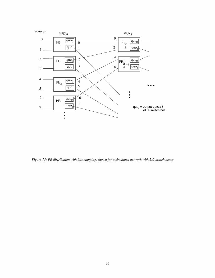
box-mapped multistage cube network consisting of 2x2 output buffered switch boxes.

Parts of stages one and two of this network are depicted in Figure 13. Assume the MP-1

global router is used. If PE0 operates on its queue quo0 while PE1 operates on its queue

quo1 and vice versa, PEN/2 receives data from only one PE per subcycle.

In general, for a box mapped network with BxB switches, consider a particular switch

box in stagei+1. Let the B PEs simulating the boxes in stagei that may send data to this

stagei+1 box be denoted P(k), where 0 ≤ k < B. Then, during subcycle j (0 ≤ j < B), PE

P(k) sends data from its output queue quok+j(mod B). If, for example, the m-th box counted

from the top of stagei is assigned to PE Pi = ( i * N/B ) + m, each PE can readily calculate

its P(k) number with k = ( Pi mod B ), and can use it to select the appropriate output

queue to send data from for each subcycle. Thus, no more than one data packet is routed

to a particular PE per subcycle. With this sequencing method and TPGEN, TSTAGE, and TBOX

defined as in Section 3.3.3, one simulation cycle requires the execution time

TCYC,box = B * TPGEN + B * TSTAGE + B * TBOX (5)

15

which is proportional to B.

3.3.5 Mapping Comparison

Consider the degree of parallelism that can be achieved with box and link mappings. In

link mapping, the inter-stage links including the network inputs and outputs are mapped

onto the PEs so that N*(s+1) PEs are needed for a sub-simulator. In box mapping, each

switch box is mapped onto a single PE, so that s*N/B PEs are needed. Thus, the number

of PEs used by a link map sub-simulator is B*(1+1/s) times the number used by a box map

sub-simulator. Considering the higher degree of parallelism and the number of inter-PE

transfers used, link mapping needs less execution time as compared to box mapping per

sub-simulator.

As mentioned above, the trade-off between the number of networks being simulated in

parallel and the speed of a network simulation is dependent upon the mapping

implementation, and must be examined by execution time measurements, as follows. The

trade-off will be illustrated by a five-stage 1024x1024 multistage cube network consisting

of 256 4x4 switch boxes per stage that is to be mapped onto a MasPar MP-1 machine with

16K PEs. Measurements show that a link-mapped sub-simulator needs 12 msec for central

memory buffering and 9.5 msec for input and output buffering per simulation cycle, while

a box-mapped sub-simulator needs 31 msec per simulation cycle for all buffering

strategies. As discussed above, a link-mapped sub-simulator requires N*(s+1) = 6144 PEs,

while s*(N/B) = 1280 PEs are needed for a box-mapped sub-simulator.

On an MP-1 with 16K PEs, either two link-mapped or 12 box-mapped sub-simulators

can run in parallel. Consider the performance of each approach with its sub-simulators

executing concurrently. Per simulation cycle, a link-mapped simulation averages 6 msec

for central memory buffering and 4.75 msec for input and output buffering, while a

box-mapped simulator averages 2.58 msec for all buffering strategies. Thus, box mapping

needs considerably less execution time per simulation cycle than link mapping, especially

during central memory buffering. Therefore, the only advantage of link mapping,

16

compared to the box mapping strategy, is the low memory requirement per PE. This

advantage is target machine and network type dependent. On the MP-1, for example, the

available memory per PE is sufficient for most practical box sizes and queue lengths (e.g.,

B = 32, li = 0, lo = 64) if short data packets are to be simulated, so that both link and box

mappings can be implemented. Because of the higher performance of box mapping, this

strategy is preferable.

Now consider the PE utilization of the two mapping strategies. For this comparison, it

is assumed that S PEs are used to implement a particular network stage (S = N for link

mapping, and S = N/B for box mapping), and that each network stage operates on uniform

traffic with load λ. The PE-utilization UPE is defined as the busy time of a PE during one

simulation cycle divided by the overall time needed for that simulation cycle (0 ≤ UPE ≤ 1).

Recall that a simulation cycle consists of the traffic pattern generation, one complete

inter-stage data transfer, and one complete intra-stage data transfer. During the data traffic

generation, only the PEs that implement the first network stage are busy, while all other

PEs involved in the network simulation are idle. Because the utilization of each PE not

involved in the pattern generation must be calculated to obtain a worst-case PE utilization

of the mappings, PEs simulating stagei with i > 0 are considered in the following.

Recall that with link mapping the intra-stage box transfers must be serialized into B

subcycles. With this mapping, λ*S PEs perform an inter-stage transfer when simulating

stagei, while λ*S/B PEs perform a switch box transfer during one intra-stage transfer

subcycle. By considering Equation (1) the utilization UPE,link over one simulation cycle of a

single PE not involved in the pattern generation can be calculated as:

.***

***

, λ

λλ

BOXSTAGEPGEN

BOXSTAGE

BOXSTAGEPGEN

BOXSTAGE

linkPE TBTTTT

TBTT

TBB

TU

+++=

++

+= (6)

Measurements with B = 4 show that with link mapping, TBOX ≈ 2.5*TSTAGE ≈ 1.5*TPGEN so

that UPE,link ≈ 0.27*λ.

17

With box mapping, λ*S PEs always perform an inter-stage transfer and a switch box

transfer in stagei. Both operations are serialized in B subcycles. By employing Equation

(5), the utilization UPE,box over one simulation cycle of a single PE not involved in the

pattern generation, with box mapping, can be therefore calculated.

.****

****

, λλλBOXSTAGEPGEN

BOXSTAGE

BOXSTAGEPGEN

BOXSTAGEboxPE TTT

TTTBTBTB

TBTBU

+++=

+++= (7)

Measurements with B = 4 show that with box mapping TBOX ≈ 0.6*TSTAGE ≈ 0.7*TPGEN so

that UPE,box ≈ 0.7*λ. These results show that, under uniform traffic, box mapping has a 2.6

times higher worst-case PE utilization than link mapping. At 80% uniform input load, for

example, box mapping utilization is 56%, while link mapping utilizes the PEs to 21%

only.

All results were derived for store-and-forward packet-switching multistage cube

network simulators. Because the mappings presented depend on the network topology

rather than on network flow control schemes, the simulators can easily be adapted to

schemes like circuit-switching, wormhole routing, or virtual channels (as already

implemented in upgraded simulator versions [11, 13]). If other network topologies, like

meshes or hypercubes, are to be simulated, mapping strategies that reflect the specific

characteristics of those topologies must be found, which is part of future work.

4. Simulator Description and Performance

The link-mapped and box-mapped simulators described in Section 3 were implemented

on the MasPar MP-1 by using the MasPar programming language MPL [3]. MPL is based

on ANSI C, with additional instructions to support data parallel programming. Each

simulation program can be divided into three main parts: (1) simulation parameter input

and network initialization, (2) a simulation itself, and (3) result collection and output.

During a simulation cycle, data packets are generated at the network inputs in accordance

18

with the selected traffic model and load. Then, a data transfer between the different stages

and the data transfer through the switch boxes is performed. During these transfers,

statistics are computed, which comprise stagewise and global average and maximum

packet delays, FIFO buffer queue utilization, and packet throughput. Separate statistics

are collected for uniform, nonuniform, and combined traffic, if a mixed traffic model is

selected. To obtain realistic simulation results, the network must be in a steady-state

condition before statistics can be gathered. Thus, warmup cycles at the beginning of a

simulation are introduced, during which no statistics are gathered. Several simulations can

be performed successively, each separated by warmup cycles, to guarantee the

independence of the trials. The results of the individual trials can be averaged and the

variance of the various results can be evaluated.

The program execution time can be calculated as:

Tsim = Tinit + ( trials ) * (warmup + cycles per trail) * Tloop + trials * Ttrialstat. (8)

Tinit accounts for the time to initialize the simulator and the random pattern generator,

Tloop represents the time needed for the execution of one simulation cycle, and Ttrialstat

accounts for the time needed to calculate the statistics after each trial. Actual

measurements of the box mapping with 12 parallel sub-simulators showed that Tinit ≅ 6

sec, Tloop ≅ 0.0026 sec, and Ttrialstat ≅ 0.056 sec.

As an example of a simulator result, the complementary distribution function of the

buffer utilization (DBU) of a five-stage 1024x1024 network with 4x4 output buffered

switches, under uniform traffic with λ = 0.7, is depicted in Figure 14. This DBU is defined

as the probability P{λo} that an output buffer with length lo will overflow at a given traffic

load. Also, the 95% confidence interval [10] of the DBU is depicted in Figure 14, so

that the actual values lie within this bound with 95% probability. The transmission of 109

packets were simulated in approximately 40 minutes. With the simulator, various network

types under static and temporary non-uniform traffic patterns were examined and classified

[11, 13].

5. Summary

19

Methods for simulating multistage interconnection networks on massively parallel

computers have been presented. Aspects of parallel simulation of networks and the impact

of the target parallel machine on the simulator implementation and performance have been

discussed. To be broadly applicable, general network and switch box models were

introduced. Different mapping strategies were studied and compared. It was shown how

the mapping granularity affects the communication overhead and the memory

requirements of the target parallel machine.

As case studies, two strategies (link and box mapping) of mapping synchronous

multistage cube networks on the MasPar MP-1 SIMD machine were compared. It was

shown how serialization and sequencing of data transfers can be used to obtain an efficient

time-driven simulator, implemented on a SIMD machine. The methods result in a

simulator implementation with which 109 data packets can be simulated in 40 minutes on

the MasPar system.

20

References

[1] R. Ayani and B. Berkman, “Parallel discrete event simulation on SIMD computers,”

Journal of Parallel and Distributed Computing, Vol. 18, No. 4, August 1993, pp.

501-508.

[2] K. E. Batcher, “Bit serial parallel processing systems,” IEEE Transactions on

Computers, Vol. C-31, No. 5, May 1982, pp. 377-384.

[3] T. Blank, “The MasPar MP-1 architecture,” IEEE Compcon, February 1990, pp.

20-24.

[4] W. Crowther, J. Goodhue, R. Thomas, W. Milliken, and T. Blackadar,

“Performance measurements on a 128-node butterfly parallel processor,” 1985

International Conference on Parallel Processing, August 1985, pp. 531-540.

[5] J. Ding and L. N. Bhuyan, “Performance evaluation of multistage interconnection

networks with finite buffers,” 1991 International Conference on Parallel

Processing, Vol. I, August 1991, pp. 592-599.

[6] D. M. Dias and J. R. Jump, “Analysis and simulation of buffered delta networks,”

IEEE Transactions on Computers, Vol. C-30, April 1981, pp. 273-282.

[7] B. Gaujal, A. G. Greenberg, and D. M. Nicol, “A sweep algorithm for massively

parallel simulation of circuit-switched networks,” Journal of Parallel and

Distributed Computing, Vol. 18, No. 4, August 1993, pp. 484-500.

[8] M. G. Hluchyj and M. J. Karol, “Queueing in high-performance packet switching,”

IEEE Journal on Selected Areas in Communications, Vol. 6, No. 9, December

1988, pp. 1587-1597.

[9] R. Hofmann and R. Mueller, “A multifunctional high speed switching element for

ATM applications,” 17th European Solid-State Conference, September 1991, pp.

237-240.

[10] E. C. Jordan, Reference Data for Engineers: Radio, Electronics, Computer, and

Communications, Howard W. Sams & Co. Inc., Indianapolis, 1985.

21

[11] M. Jurczyk and T. Schwederski, “On partially dilated multistage interconnection

networks with uniform traffic and nonuniform traffic spots,” 5th IEEE Symposium

on Parallel and Distributed Processing, December 1993, pp. 788-795.

[12] M. Jurczyk and T. Schwederski, “SIMD processing: Concepts and systems” in

Handbook of Parallel and Distributed Computing, A. Y. Zomaya, ed., McGraw-

Hill, New York, NY, 1995.

[13] M. Jurczyk and T. Schwederski, “Phenomenon of higher order head-of-line blocking

in multistage interconnection networks under nonuniform traffic patterns,” IEICE

Transactions on Information and Systems, Vol. E79-D, No. 8, August 1996, pp.

1124-1129.

[14] M. J. Karol, M. G. Hluchyj, and S. P. Morgan, “Input versus output queueing on a

space-division packet switch,” IEEE Transactions on Communications, Vol. COM-

35, No. 12, December 1987, pp. 1347-1356.

[15] N. Koike, “NEC Cenju-3: A microprocessor-based parallel computer multistage

network,” 8th International Parallel Processing Symposium, April 1994, pp. 393-

401.

[16] D. H. Lawrie, “Access and alignment of data in an array processor,” IEEE

Transactions on Computers, Vol. C-24, No. 12, December 1975, pp. 1145-1155.

[17] K. J. Liszka, J. K. Antonio, and H. J. Siegel, “Problems with comparing

interconnection networks: Is an alligator better than an armadillo?," IEEE

Concurrency, Vol. 5, No. 4, Oct.-Dec. 1997, pp. 18-28.

[18] Y.-S. Liu and S. Dickey, “Simulation and analysis of different switch architectures

for interconnection networks in MIMD shared memory machines,” Ultracomputer

Note 141, NYU, June 1988, pp. 1-26.

[19] M. C. Pease III, “The indirect binary n-cube microprocessor array,” IEEE

Transactions on Computers, Vol. C-26, No. 5, May 1977, pp. 458-473.

[20] D. A. Reed and R. M. Fujimoto, Multicomputer Networks: Message-based Parallel

Processing, MIT Press, Cambridge, MA, 1987.

22

[21] T. Schwederski and M. Jurczyk, Interconnection Networks: Structures and

Properties (in German), Teubner Verlag, Stuttgart, Germany, 1996.

[22] H. J. Siegel, Interconnection Networks for Large-Scale Parallel Processing: Theory

and Case Studies, Second Edition, McGraw-Hill, New York, NY, 1990.

[23] H. J. Siegel, W. G. Nation, C. P. Kruskal, and L. M. Napolitano, “Using the

multistage cube network topology in parallel supercomputers,” Proceedings of the

IEEE, Vol. 77, No. 12, December 1989, pp. 1932-1953.

[24] H. J. Siegel, T. Schwederski, W. G. Nation, J. B. Armstrong, L. Wang, J. T. Kuehn,

M. D. Gupta, M. D. Allemang, D. G. Meyer, and D. W. Watson, “The design and

prototyping of the PASM reconfigurable parallel processing system” in Parallel

Computing: Paradigms and Applications, A. Y. Zomaya, ed., International

Thomson Computer Press, London, 1995, pp. 78-114.

[25] H. J. Siegel and C. B. Stunkel, “Inside parallel computers: Trends in interconnection

networks,” IEEE Computational Science and Engineering, Vol. 3, No. 3, Fall

1996, pp. 69-71.

[26] C. B. Stunkel, D. G. Shea, B. Abali, M. G. Atkins, C. A. Bender, D. G. Grice, P.

Hochschild, D. J. Joseph, B. J. Nathanson, R. A. Swetz, R. F. Stucke, M. Tsao, and

P. R. Varker, “The SP2 high-performance switch,” IBM Systems Journal, Vol. 34,

No. 2, 1995, pp. 185-202.

[27] S. Thanawastien and V. P. Nelson, “Interference analysis of shuffle/exchange

networks,” IEEE Transaction on Computers, Vol. C-30, No. 8, August 1981, pp.

545-556.

[28] L. W. Tucker and G. G. Robertson, “Architecture and applications of the

Connection Machine,” Computer, Vol. 21, No. 8, August 1988, pp. 26-38.

[29] M.-C. Wang, H. J. Siegel, M. A. Nichols, and S. Abraham, “Using a multipath

network for reducing the effect of hot spots,” IEEE Transactions on Parallel and

Distributed Systems, Vol. 6, No. 3, March 1995, pp. 252-268.

[30] F. Wieland and D. Jefferson, “Case studies in serial and parallel simulation,” 1989

23

International Conference on Parallel Processing, Vol. III, August 1989, pp. 255-

258.

[31] C.-L. Wu and T. Y. Feng, “On a class of multistage interconnection networks,”

IEEE Transactions on Computers, Vol. C-29, No. 8, August 1980, pp. 694-702.

24

Figure Captions:

Figure 1: General unidirectional multistage interconnection network model

Figure 2: Switch box model

Figure 3: (a) output buffered switch with input latches, (b) input buffered switch, and (c)

central memory switch

Figure 4: SIMD machine model

Figure 5: Mappings with different granularity: (a) fine, (b) medium, and (c) coarse

granularity mapping

Figure 6: Trade-offs of mappings with different granularity

Figure 7: A 16x16 multistage cube network with 4x4 switch boxes

Figure 8: PE-interconnection structure of the MasPar MP-1 machine [3]

Figure 9: Mapping of PEs on a BxB switch box with link mapping, shown for B=4

Figure 10: Routing conflict in a 2x2 switch box

Figure 11: Part of the inter-stage connection pattern pf a multistage cube network

Figure 12: Mapping of PEs on a BxB switch box with box mapping, shown for B=4

Figure 13: PE distribution with box mapping, shown for a simulated network with 2x2

switch boxes

Figure 14: Complementary queue length distribution function DBU of a 1024x1024

network with 4x4 output buffered switch boxes, under uniform traffic with λ=0.7

25

Figure 1: General unidirectional multistage interconnection network model

network

= data path

= control path

stage cntrl

Si = source i Di = destination i

network control

S0

S1

SN-1

stage0

stag

e in

terc

onne

ctio

nbox0

switch

box1

switch

boxb-1

switch

stag

e in

terc

onne

ctio

n

box0

switch

box1

switch

boxb-1

switch

stage1

stage cntrl

stag

e in

terc

onne

ctio

n

box0 switch

box1 switch

boxb-1

switch

stages-1

stage cntrl

D0

D1

DN-1

26

Figure 2: Switch box model

outputqueueqo-1

queue control

outputqueue1

queue control

outputqueue0

queue control

switch box

port0

port1

portpi-1inputqueueqi-1

queue control

inputqueue1

queue control

inputqueue0

queue control

box control

inpu

t por

ts

switc

h ro

utin

g un

it

outp

ut p

orts

port0

port1

portpo-1

= data path= control path

27

Figure 3: (a) output buffered switch with input latches, (b) input buffered switch, and (c) central memory

switch

(a)

= buffer queue= crossbar switch= latch

(b) (c)

MUX=multiplexor

DMUX=demultiplexor

MU

X

DM

UX

RAM

28

Figure 4: SIMD machine model

control unit

proc1

mem1

PE0

proc = processor

mem = memory

interconnection network

PE1S

PEN -1

proc0

mem0

SprocN -1

SmemN -1

29

Figure 5: Mappings with different granularity: (a) fine, (b) medium, and (c) coarse granularity mapping

= link= switch box= PE

fine granularity medium granularity coarse granularityPE per link PE per box PE per T boxes

PE PEPE

(a) (b) (c)

PEPE

PE

PEPE

PE

PE

PE

PE PE

30

Figure 6: Trade-offs of mappings with different granularity

fine granularity medium granularity coarse granularity

PE per link PE per box PE per T boxes

Ad./Dis.

Ad./Dis.

Ad./Dis.

Ad./Dis.= advantage/disadvantage‡ The network input and output links must be mapped as well → s+1.

number of PEs used persub-simulator

execution time per simulation

inter-PE communication requirement

memory requirement per PE

overhead of box operations (e.g., for central memory buffering)

number of network sub-simulators

running inparallel

+

-

high

N*(s+1)

N*(s+1)

‡

low

low

low

high

high

+

-

-

NS

medium

medium

medium

medium

low

N*sB

medium

+

N*s

NS*B

-

±

±

±

+

-

+

+

-

low

low

high

high

high

low

N*s

NS*B*T

T*B

N*s

NxN network with BxB boxes consisting of s stages mapped onto a SIMD machine with NS processors

(N is a multiple of B)

31

Figure 7: A 16x16 multistage cube network with 4x4 switch boxes

sources destinations

stage 0 1

0

15

0

15

32

Figure 8: PE-interconnection structure of the MasPar MP-1 machine [3]

S1

S2

S3

three-stageglobal router

PEcluster

X-Net

33

Figure 9: Mapping of PEs on a BxB switch box with link mapping, shown for B=4

IB

OB

OB

IB

PEiPEn

PEp

PEr

OB

IBOB

IB

OB IB

OB IB

OB

IB

switch box

OB

IB

PEj

PEk

PEm

PEq

OB = output buffer IB = input buffer = PE

34

Figure 10: Routing conflict in a 2x2 switch box

switch boxi

= output buffer = input buffer = PEquiiquoi

PEi PEk

PEmPEj

stagej

quo0

quo1

qui0

qui1

35

Figure 11: Part of the inter-stage connection pattern pf a multistage cube network

stagei

B box0

boxB-1

boxB

boxN/B-1

box1

box0

box1B

B

B

B

B

B

B

B

B

B

B

B

B

B

B

B

B

B

B

B

B

boxN/B-1

stagei+1

boxN/B -12

boxN/B 2

box2N/B -12

gri+1= 0

gri+1= 1

36

Figure 12: Mapping of PEs on a BxB switch box with box mapping, shown for B=4

OB

OB

OB

OB

IB

IB

IB

IB

switch box

OB = output buffer IB = input buffer = PE

PE

37

Figure 13: PE distribution with box mapping, shown for a simulated network with 2x2 switch boxes

stage0

PE0quo0

quoi = output queue i of a switch box

sources

0

1

2

3

4

5

6

7

2+1

0

1

23

45

67

0

2

4

6

quo1

quo0

quo1

quo0

quo1

quo0

quo1

quo0

quo1

quo0

quo1

stage1

PE1

PE2

PE3

PEN

PEN

2

38

Figure 14: Complementary queue length distribution function DBU of a 1024x1024 network with 4x4

output buffered switch boxes, under uniform traffic with λ=0.7

1.00E-08

1.00E-07

1.00E-06

1.00E-05

1.00E-04

1.00E-03

1.00E-02

1.00E-01

1.00E+000 4 8 12 16 20 24

output buffer length l 0DBU (log scale)

+ = stage1

= stage5