strategic delay in a real options model of r&d …
TRANSCRIPT

STRATEGIC DELAY IN A REAL OPTIONS MODELOF R&D COMPETITION
Helen Weeds
No 576
WARWICK ECONOMIC RESEARCH PAPERS
DEPARTMENT OF ECONOMICS

STRATEGIC DELAY IN A REAL OPTIONS
MODEL OF R&D COMPETITION
HELEN WEEDS
Department of Economics, University of Warwick
20 September 2000
Abstract
This paper considers irreversible investment in competing research projects withuncertain returns under a winner-takes-all patent system. Uncertainty takes twodistinct forms: the technological success of the project is probabilistic, while theeconomic value of the patent to be won evolves stochastically over time. Accordingto the theory of real options uncertainty generates an option value of delay, but withtwo competing firms the fear of preemption would appear to undermine thisapproach. In non-cooperative equilibrium two patterns of investment emergedepending on parameter values. In a preemptive leader-follower equilibrium firmsinvest sequentially and option values are reduced by competition. A symmetricoutcome may also occur, however, in which investment is more delayed than thesingle-firm counterpart. Comparing this with the optimal cooperative investmentpattern, investment is found to be more delayed when firms act non-cooperatively,as each holds back from investing in the fear of starting a patent race. Implicationsof the analysis for empirical and policy issues in R&D are considered.
JEL classification numbers: C61, D81, L13, O32.Keywords: real options, preemption, R&D, investment.Address: Department of Economics, University of Warwick, Coventry CV4 7AL, UK.Tel: (024) 76 523052; fax: (024) 76 523032; e-mail: [email protected]__________________________________________The author would like to thank Martin Cripps, Chris Harris, Dan Maldoom, Robin Mason, RobertPindyck, Hyun Shin, John Vickers and two anonymous referees for their comments and suggestions.All errors remain the responsibility of the author.

1
Strategic Delay in a Real Options Model of R&D Competition
1 Introduction
When a firm has the opportunity to make an irreversible investment facing future uncertainty
there is an option value of delay. By analogy with a financial call option it is optimal to delay
exercising the option to invest, even when it would be profitable to do so at once, in the
hope of gaining a higher payoff in the future. Using this insight the real options approach
improves upon traditional NPV-based investment appraisal methods by allowing the value
of delay and the importance of flexibility to be quantified and incorporated explicitly into the
analysis.
Real world investment opportunities, unlike financial options, are rarely backed by legal
contracts which guarantee the holder’s rights in precise terms. Most real options are non-
proprietary investment opportunities whose terms are somewhat vague or subjective, and far
from guaranteed. In particular, a firm’s ability to hold the option is frequently influenced by
the possibility that another firm may exercise a related option, which affects the value of the
first firm’s investment. In a few instances a legal right such as an oil lease or a patent gives a
firm a proprietary right similar to that granted by a financial option. Or occasionally a firm
has such a strong market position, as in a natural monopoly or network industry, that its
investment opportunities are de facto proprietary. However, in most industries some
degree of competition exists, either actual or potential, and the option to invest cannot be
held independently of strategic considerations.
When a small number of firms are in competition with an advantage to the first mover,
each one’s ability to delay is undermined by the fear of preemption. Consider a situation in
which two firms have the ability to exercise an option and the first to do so obtains the
underlying asset in its entirety, leaving the second mover empty-handed. Each firm would
like to exercise the option just before its rival does so, giving rise to discontinuous Bertrand-
style reaction functions. With symmetric firms the value of delay is eliminated and the option
will be exercised as soon at the payoff from doing so becomes marginally positive. Under

2
such circumstances the real options approach becomes irrelevant and the traditional NPV
rule resurfaces as the appropriate method of investment appraisal.
In order to study in detail the tension between real options and strategic competition, the
continuous time framework of Fudenberg and Tirole (1985) is adapted in two important
respects to apply to the specific context of rival investment in R&D. The firms’ profit
functions are specified so as to include two distinct forms of uncertainty: economic
uncertainty over the future profitability of the project, and technological uncertainty over the
success of R&D investment itself. Economic uncertainty gives rise to option values and a
tendency for delay, which would not arise in a deterministic framework. Technological
uncertainty, combined with a winner-takes-all patent system, generates a preemption effect
that counteracts the incentive to delay. The instantaneous probability of success, or hazard
rate, of rival firms captures in a simple form the strength of the first-mover advantage,
allowing outcomes for varying degrees of preemption to be readily compared. In effect,
technological uncertainty drives a wedge between a firm’s decision to invest and the out-turn
of that investment, giving some scope for the follower to leapfrog the leader and preserving
its option value to some extent. It should be noted that the advantage gained by the first
mover is not necessarily a persistent one: if the breakthrough is not achieved before the
follower invests, the two firms are equally likely to succeed from then on.
In fact, the hazard rate has two distinct effects in this model. The direct effect of the
rival’s hazard rate is to reduce the expected value of investment to the second mover, since
there is some probability that the leader will make the discovery first. This effect is
analogous to the impact of rival investment in product market duopoly models such as Smets
(1991): with the option value of delay unchanged, the reduction in the value of investment
causes the follower to act later. In this paper, however, there is also a second effect: the
hazard rate of rival innovation reduces the option value itself, tending to hasten investment.
Thus option values and preemption interact in this model. This contrasts with existing
contributions in the area, where the roles of option values and competition are additive: in
these models the only effect of rivalry is to reduce the value of investment, while the option
value of delay remains unchanged.
3
Focusing on Markov perfect equilibria, the outcome of the non-cooperative two-player
game takes one of two forms depending upon parameter values. The first is a preemptive
leader-follower outcome in which one firm invests strictly earlier than the other and option
values are undermined by competition. The second has a multiplicity of equilibria, including
a continuum of symmetric equilibria in which both firms invest at the same trigger point. The
Pareto-dominant equilibrium coincides with the optimal joint-investment rule which would be
chosen by firms that agree to adopt a common trigger point. This outcome entails greater
delay than the single-firm counterpart.
The role of the hazard rate in non-cooperative equilibrium can be understood as follows.
Its impact in lowering the expected value of investment to the second-mover, relative to the
firm that invests first, creates a first-mover advantage that will tend to induce preemptive
action. However, when the first firm invests the value of its rival’s option to delay is also
reduced, speeding up the competitive reaction to its investment. Thus, preemption is
double-edged: the leader gains a privileged position for a time, but the option value effect
tends to speed up the reaction of its competitor. Anticipating this reaction, a firm may
instead choose to delay its own investment. In effect, an investing firm chooses the time at
which the patent race will begin and it is better for each firm if this is delayed until the optimal
joint-investment point is reached. A good analogy is the behaviour of contestants in a long-
distance race, who typically remain in a pack proceeding at a moderate pace for most of the
distance, until near the end when someone attempts to break away and the sprint for the
finish begins. Compared with existing duopoly models of real options the cooperative joint-
investment outcome is achievable as a non-cooperative equilibrium.
The fully optimising cooperative investment rule is derived as a benchmark for
comparison. This is shown to involve sequential investment of the two units, so that research
efforts are phased in over time. Compared with the non-cooperative leader-follower
equilibrium, the cooperative trigger points are higher than their non-cooperative counterparts
since option values are no longer undermined by preemption. The non-cooperative joint-
investment equilibrium, although preferable to the preemptive leader-follower outcome, is
seen not to be the fully-optimising choice of cooperating firms. It may, however, be
interpreted as the second-best optimum of firms that are constrained to choose a symmetric
4
investment rule, given the difficulty of agreeing an asymmetric investment pattern or making
side-payments to support the fully-optimising solution. It is interesting to note that when
simultaneous investment is the equilibrium outcome, the time to first investment is increased
by strategic interactions between non-cooperative firms, compared with the cooperative
solution.
By combining irreversible investment under uncertainty with strategic interactions in the
presence of technological uncertainty, the paper brings together three strands of economics
literature. Real options models have been used to explain delay and hysteresis arising in a
number of contexts, but these are mostly set in a monopolistic or perfectly competitive
framework. McDonald and Siegel (1986) and Pindyck (1988) consider irreversible
investment opportunities available to a single firm. Dixit (1989, 1991) considers product
market entry and exit in, respectively, monopolistic and perfectly competitive settings. The
second branch of related literature analyses timing games of entry and exit in a deterministic
framework. Timing games are straightforward examples of stopping time games where the
underlying process is simply time itself. Papers analysing preemption games include
Fudenberg et al. (1983) and Fudenberg and Tirole (1985), while wars of attrition have been
modelled by Ghemawat and Nalebuff (1985) and Fudenberg and Tirole (1986). Finally,
technological uncertainty in R&D, with discovery modelled as a Poisson arrival, is
considered in papers by, inter alia, Loury (1979), Dasgupta and Stiglitz (1980), Lee and
Wilde (1980), Reinganum (1983) and Dixit (1988). These papers, however, assume the
return to successful R&D (or demand in the product market from which it is derived) to be
deterministic, thus ruling out any option value of delay and related timing issues.
Existing literature combining real options with strategic interactions is as yet relatively
limited. Smets (1991; summarised in Dixit and Pindyck 1994, pp. 309-314), examines
irreversible market entry for a duopoly facing stochastic demand. Non-cooperative
behaviour results in an asymmetric leader-follower equilibrium. When the leadership role is
exogenously pre-assigned so that the follower is unable to invest until after the designated
leader has done so, the cooperative symmetric outcome may then be attained. Grenadier
(1996) considers the strategic exercise of options applied to real estate markets. Joint
investment arises only when the underlying stochastic process starts at a sufficiently high

5
initial value and, even then, is not necessarily undertaken at the optimal point. In a two-
player game where each player’s exercise cost is private information, Lambrecht and
Perraudin (1997) find trigger points located somewhere between the monopoly and simple
NPV outcomes. In a two-period model, Kulatilaka and Perotti (1998) consider the value
of strategic investment as the degree of uncertainty increases.
The paper is structured as follows. The model is described in section 2. The
optimisation problem of a single firm facing no actual or potential competition is solved in
section 3. Section 4 derives the optimal cooperative investment plan for two firms. Non-
cooperative equilibrium in the two-player game is found in section 5. The findings are
discussed in section 6; section 7 then concludes.
2 The model
Two risk-neutral firms, i = 1, 2, have the opportunity to invest in competing research
projects. Research is directly competitive: the firms strive for the same patent and successful
innovation by one eliminates all possible profit for the other. The firms face both
technological and economic uncertainty. Discovery by an active firm is a Poisson arrival,
while the value of the patent received by the successful inventor evolves stochastically over
time.1 The decision to invest in a research project is assumed to be irreversible. The
possible states of firm i are denoted { }1 ,0 ∈iθ for the idle and active states respectively.
The value of the patent, π , evolves exogenously and stochastically according to a
geometric Brownian motion (GBM) with drift given by the following expression
dWdtd ttt σπµππ += (1)
where µ ∈ [0, r) is the drift parameter measuring the expected growth rate of π ,2
r is the risk-free interest rate, assumed to be constant over time, σ > 0 is the instantaneous
standard deviation or volatility parameter, and dW is the increment of a standard Wiener
process where dW ∼ N(0, dt).

6
Each firm has the opportunity to invest in a research project. Following Loury (1979),
firm i sets up a research project by investing an amount 0>iK .3 From the time of this
investment, discovery takes place randomly according to a Poisson distribution with
constant hazard rate 0>ih . Thus the hazard rate is independent of the duration of research
and the number of firms investing; possible variations on this assumption are discussed in
section 7. The probabilities of discovery by each firm are independent. We focus on the
symmetric case where hhi = and KK i = for i = 1, 2. All parameter values and actions
are common knowledge, thus the game is one of complete information.
The following assumptions are made
Assumption 1. ( ) 0
0
0 <−
∫
∞ +− KdtheE tthr π .
Assumption 2. If ( ) 1=τθ i then ( ) 1=tiθ τ≥∀t .
Assumption 1 states that the initial value of the patent, 0π , is sufficiently low that the
expected return from immediate investment is negative, ensuring that neither firm will invest
at once. Assumption 2 formalises the irreversibility of investment and constrains the strategy
of the firm accordingly: if firm i has already invested by date τ then it remains active at all
dates subsequent to τ until the game ends with a discovery.
In a multi-agent setting the firm’s investment problem can no longer be solved using the
optimisation techniques typically employed in real options analysis. Instead, the optimal
control problem becomes a stopping time game (for a detailed analysis see Dutta and
Rustichini (1991)). In a stopping time game each player has an irreversible action such that,
following this action by one or more players, expected payoffs in the subsequent subgame
are fixed. Dutta and Rustichini allow for the possibility that the stochastic process continues
to evolve after the leader’s action and that the follower still has a move to make, as is the
case in this paper. The stopping time game is described by the stochastic process π along
with the payoff functions for the leader and follower; these are derived in section 5 below.
The game proceeds as follows. In the absence of action taken by either firm, the
stochastic process evolves according to (1). If firm i has not commenced research at any
time t<τ its action set is { }investt don' invest, =itA . If, on the other hand, i has invested
7
at some t<τ , then itA is the null action set { }movet don' . Thus each firm faces a control
problem in which its only choice is when to choose the action ‘stop’ – or rather, in this case,
to start research. After taking this action the firm can make no further moves to influence the
outcome of the game. The game ends when a discovery is made by either firm.
A strategy for firm i is a mapping from the history of the game tH to the action set itA
as follows: itt
it AH →:σ . At time t ≥ 0, the history of the game has two components, the
sample path of the stochastic state variable π and the actions of the two firms up to date t.
With irreversible investment the history of actions in the game at t is summarised by the fact
that the game is still continuing at t (i.e. 0=iθ i∀ ). However, the history of the state
variable is more complex since its current value could have been reached by any one of a
huge number of possible paths.
Firms are assumed to employ stationary Markovian strategies: actions are functions of
the current state alone and the strategy formulation itself does not vary with time. Since the
state variable π follows a Markov process, Markovian strategies incorporate all payoff-
relevant factors in the game. Furthermore, if one player uses a Markovian strategy then its
rival has a best response that is Markovian as well. Hence a Markovian equilibrium remains
an equilibrium when history-dependent strategies are also permitted, although other non-
Markovian equilibria may then also exist. For further explanation see Maskin and Tirole
(1988) and Fudenberg and Tirole (1991, chapter 13). With the Markovian restriction a
player’s strategy is a stopping rule specifying a critical value or “trigger point” for the
stochastic variable π at which the firm invests.4
As Fudenberg and Tirole (1985) point out, the use of continuous time complicates the
formulation of strategies as there is a loss of information inherent in taking the limit of a
discrete time mixed strategy equilibrium. To deal with this problem they extend the strategy
space to include not only the cumulative probability that a player has adopted, but also the
“intensity” with which a player adopts “just after” the cumulative probability has jumped to
one. Although this formulation uses symmetric mixed strategies, equilibrium outcomes are
equivalent to those in which firms employ pure strategies and may adopt asymmetric roles.5
Thus, although the underlying framework is an extended space with symmetric mixed

8
strategies, the analysis will proceed as if each firm uses a (possibly asymmetric) pure
Markov strategy.
3 Optimal investment timing for a single firm
We start by deriving the optimal stopping time for a single firm investing in the absence of
competition. The firm’s investment rule is found by solving the stochastic optimal stopping
problem
( ) ( )
−= ∫
∞ +−− KdheeEVT
hrrTtTt τππ τ
τ max
(2)
where Et denotes expectations conditional on information available at time t and T is the
unknown future stopping time at which the investment is made. The value function ( )πV has
two distinct components which hold over different intervals of π . Let ( )π0V denote the
value function before the firm invests, and ( )π1V denote the value function after investment
has taken place.
Prior to investment the firm holds the option to invest. It has no cashflows but may
experience a capital gain or loss on the value of this option. Hence, in the continuation
region (values of π for which it is not yet optimal to invest) the Bellman equation for the
value of the investment opportunity is given by
( )00 dVEdtrV = . (3)
Using Itô’s lemma and the GBM equation (1) yields the ordinary differential equation
( ) ( ) 0 21
00022 =−′+′′ rVVV πµπππσ . (4)
From (1) it can be seen that if π ever goes to zero it stays there forever. Therefore the
option to invest has no value when 0=π and ( )π0V must satisfy the boundary condition

9
( ) 000 =V . Solving the differential equation (4) subject this boundary condition gives the
value of the option to invest in research
( ) 000
βππ BV = (5)
where 00 ≥B is an unknown constant and 0β is the positive root of the characteristic
equation 02
2
1 222 =−
−−
σε
σµ
εr
, i.e. 182
12
121
2
2
220 >
+
−+−=
σσµ
σµ
βr
.
We next consider the value of the firm in the stopping region (values of π for which is it
optimal to invest at once). Since investment is irreversible the value of the firm in the
stopping region, ( )π1V , is given by the project expected value alone with no option value
terms. Recalling that discovery is a Poisson arrival, the expected value of the active project
when the current value of the stochastic process is tπ is given by
( ) ( )
= ∫
∞ +− τππ ττ dheEV
t
hrtt
1 . (6)
Recalling that π is expected to grow at rate µ and suppressing time subscripts we can write
( )µ
ππ
−+=
hrh
V1 . (7)
Note that the hazard rate h enters the denominator in this expression in the form of an
‘augmented discount rate’ hr + . This result is typical of models involving a Poisson arrival
function: for other examples of this characteristic in the context of R&D see, inter alia,
Loury (1979), Dasgupta and Stiglitz (1980), Lee and Wilde (1980) and Dixit (1988).
The optimal investment rule is found by solving for the boundary between the
continuation and stopping regions. This boundary is given by a critical value of the
stochastic process, or trigger point, Uπ such that continued delay is optimal for
Uππ < and immediate investment is optimal for Uππ ≥ . The optimal stopping time UT is

10
then defined as being the first time that the stochastic process π hits the interval
[ )∞,Uπ . By arbitrage, the critical value must satisfy the value-matching condition
( ) ( ) KVV UU −= ππ 10 . (8)
Optimality requires a second condition known as smooth-pasting to be satisfied. This
condition requires the value functions ( )π0V and ( )π1V to meet smoothly at Uπ with equal
first derivatives6
( ) ( )UU VV ππ 10 ′=′ . (9)
Conditions (8) and (9) together imply that
( )( )
Khhr
Uµ
ββ
π−+
−=
10
0 ; (10)
and
( ) 0
1
0
0
βµπ β
−+=
−
hrh
B U . (11)
The optimal investment time at which the single firm invests is thus defined as
{ }UU tT ππ ≥≥= :0inf . (12)
Briefly considering the properties of the trigger point Uπ , as economic uncertainty is
eliminated (i.e. as σ → 0), 0β → r/µ and the optimal stopping point approaches the
breakeven value of the patent calculated on a simple NPV basis. As uncertainty rises 0β
falls towards unity, raising Uπ and increasing the expected stopping time. Thus greater
uncertainty over patent value delays investment, as expected from the papers by McDonald
and Siegel (1986), Pindyck (1988) and Dixit (1989).

11
4 The cooperative benchmark
We next consider the benchmark case in which the two firms (or research units) plan their
investments cooperatively.7 The cooperative investment pattern may (in theory at least) take
one of two possible forms: either both units invest at a single trigger point, or they invest
sequentially at distinct trigger points. We start by deriving the optimal joint-investment rule
when firms invest at the same trigger point, which follows straightforwardly from the analysis
of section 3. The optimal sequential investment plan is then derived and compared with the
optimal joint-investment strategy in order to determine which investment pattern forms the
cooperative optimum.
The analysis of the preceding section can be readily extended to the case of two
cooperating firms (or research units under common ownership) which agree to adopt a
common investment rule. The decision is equivalent to a single firm optimisation problem
with an investment cost of 2K and arrival rate 2h. Denoting the optimal joint-investment
trigger point by Cπ , value-matching and smooth-pasting conditions are used as before to
yield
( )( )
Khhr
Cµ
ββ
π−+
−=
210
0 . (13)
The optimal joint investment time CT is analogous to expression (12). As before, the
value of a (single) firm under this scenario has two parts. Prior to investment the firm holds
the option to invest; after (joint) investment the value of the active project is given by its
expected NPV to the firm, taking account of the fact that the other firm is also active, which
is
( )µ
ππ
−+=
hrh
NPV2
. (14)
Thus, the value of an individual firm under this scenario is described by the following value
function (i.e. the combined firm consisting of two research units has twice this value)
12
( )( )
≥−
<=
C
CC
C
KNPV
BV
πππ
ππππ
β
for
for 0
(15)
where ( ) 0
1
2
0
βµπ β
−+=
−
hrh
B CC .
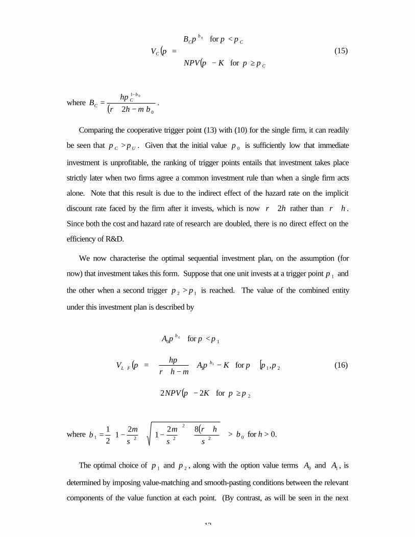
Comparing the cooperative trigger point (13) with (10) for the single firm, it can readily
be seen that UC ππ > . Given that the initial value 0π is sufficiently low that immediate
investment is unprofitable, the ranking of trigger points entails that investment takes place
strictly later when two firms agree a common investment rule than when a single firm acts
alone. Note that this result is due to the indirect effect of the hazard rate on the implicit
discount rate faced by the firm after it invests, which is now hr 2+ rather than hr + .
Since both the cost and hazard rate of research are doubled, there is no direct effect on the
efficiency of R&D.
We now characterise the optimal sequential investment plan, on the assumption (for
now) that investment takes this form. Suppose that one unit invests at a trigger point 1π and
the other when a second trigger 12 ππ > is reached. The value of the combined entity
under this investment plan is described by
( ) [ )
( )
≥−
∈−+−+
<
=+
for 22
,for
for
2
211
10
1
0
πππ
ππππµ
π
πππ
π β
β
KNPV
KAhrh
A
V FL (16)
where ( )
+
+
−+−= 2
2
22182
12
121
σσµ
σµ
βhr
> 0β for h > 0.
The optimal choice of 1π and 2π , along with the option value terms 0A and 1A , is
determined by imposing value-matching and smooth-pasting conditions between the relevant
components of the value function at each point. (By contrast, as will be seen in the next
13
section, no smooth-pasting obtains at the leader’s investment trigger in the non-cooperative
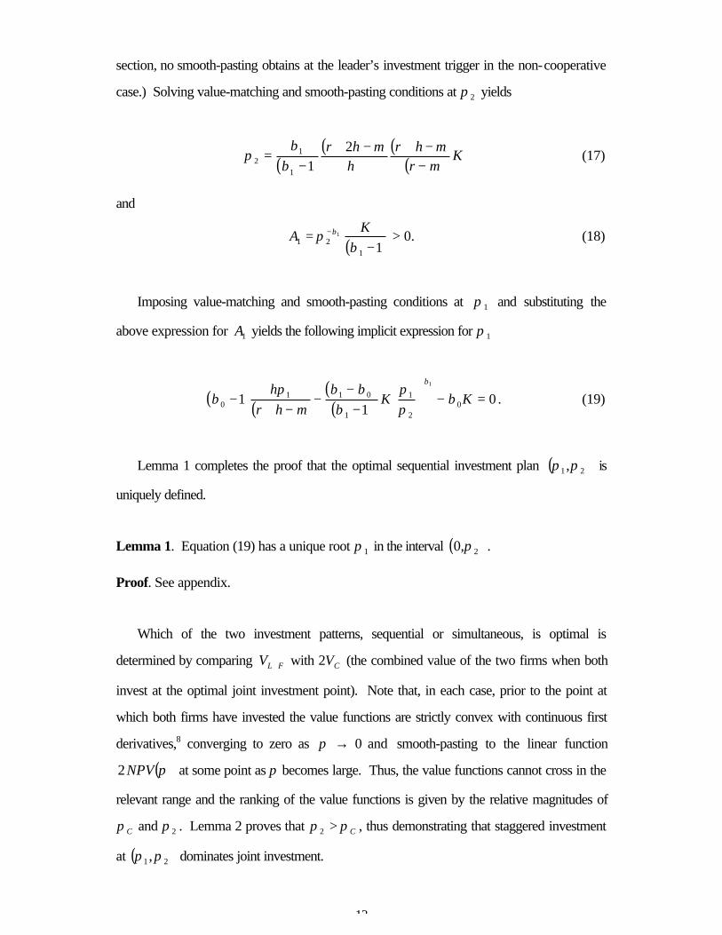
case.) Solving value-matching and smooth-pasting conditions at 2π yields
( )( ) ( )
( ) Krhr
hhr
µµµ
ββ
π−−+−+
−=
2
11
12 (17)
and
( )1121
1
−= −
βπ β K
A > 0. (18)
Imposing value-matching and smooth-pasting conditions at 1π and substituting the
above expression for 1A yields the following implicit expression for 1π
( ) ( )( )( ) 0
11 0
2
1
1
0110
1
=−
−
−−
−+− KK
hrh
βππ
βββ
µπ
ββ
. (19)
Lemma 1 completes the proof that the optimal sequential investment plan ( )21 ,ππ is
uniquely defined.
Lemma 1. Equation (19) has a unique root 1π in the interval ( )2,0 π .
Proof. See appendix.
Which of the two investment patterns, sequential or simultaneous, is optimal is
determined by comparing FLV + with 2 CV (the combined value of the two firms when both
invest at the optimal joint investment point). Note that, in each case, prior to the point at
which both firms have invested the value functions are strictly convex with continuous first
derivatives,8 converging to zero as π → 0 and smooth-pasting to the linear function
( )πNPV2 at some point as π becomes large. Thus, the value functions cannot cross in the
relevant range and the ranking of the value functions is given by the relative magnitudes of
Cπ and 2π . Lemma 2 proves that Cππ >2 , thus demonstrating that staggered investment
at ( )21 ,ππ dominates joint investment.

14
Lemma 2. Cππ >2 for h > 0.
Proof. See appendix.
Proposition 1 follows directly from the preceding analysis.
Proposition 1. The cooperative optimum is uniquely defined as a sequential
investment pattern in which one research unit invests at 1π and the other at 2π ,
where these trigger points satisfy (19) and (17) respectively.
Next we compare the trigger points in the optimal cooperative investment pattern with
the optimal joint-investment trigger Cπ .
Lemma 3. 1ππ >C for h > 0.
Proof. See appendix.
Proposition 2. The ranking of trigger points in the optimal cooperative investment
plan relative to the optimal joint-investment trigger point is given by 21 πππ << C .
Proof. Follows directly from lemmas 2 and 3.
Thus, we have demonstrated that two cooperating firms which jointly optimise their
investments would choose to phase their R&D investments progressively over time, rather
than invest both research units at once. This is despite the fact that the cost function for
research displays constant returns to scale, albeit with a given minimum size of a research
unit. The sequential investment pattern gives the possibility of some return even when the
value of innovation is fairly low (though NPV-positive), reducing the opportunity cost of
delay while holding back from committing all R&D costs at once and retaining an option to
increase the scale of investment in the future. The phasing of investment gives the
cooperating firms a higher probability of gaining a high-valued patent, and the overall value
of the (combined) investment opportunity is thereby maximised.
15
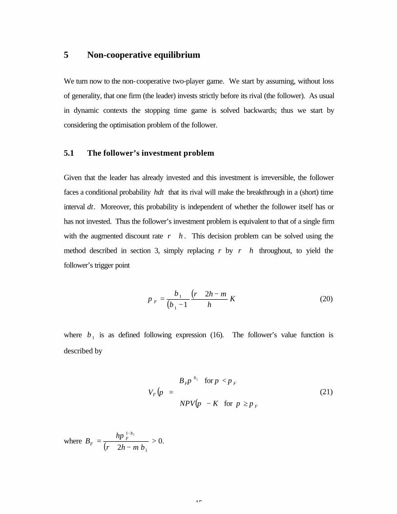
5 Non-cooperative equilibrium
We turn now to the non-cooperative two-player game. We start by assuming, without loss
of generality, that one firm (the leader) invests strictly before its rival (the follower). As usual
in dynamic contexts the stopping time game is solved backwards; thus we start by
considering the optimisation problem of the follower.
5.1 The follower’s investment problem
Given that the leader has already invested and this investment is irreversible, the follower
faces a conditional probability hdt that its rival will make the breakthrough in a (short) time
interval dt. Moreover, this probability is independent of whether the follower itself has or
has not invested. Thus the follower’s investment problem is equivalent to that of a single firm
with the augmented discount rate hr + . This decision problem can be solved using the
method described in section 3, simply replacing r by hr + throughout, to yield the
follower’s trigger point
( )( )
Khhr
Fµ
ββ
π−+
−=
211
1 (20)
where 1β is as defined following expression (16). The follower’s value function is
described by
( )( )
≥−
<=
F
FF
F
KNPV
BV
πππ
ππππ
β
for
for 1
(21)
where ( ) 1
1
2
1
βµπ β
−+=
−
hrh
B FF > 0.
16
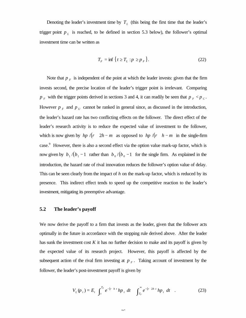
Denoting the leader’s investment time by LT (this being the first time that the leader’s
trigger point Lπ is reached, to be defined in section 5.3 below), the follower’s optimal
investment time can be written as
{ }FLF TtT ππ ≥≥= : inf . (22)
Note that Fπ is independent of the point at which the leader invests: given that the firm
invests second, the precise location of the leader’s trigger point is irrelevant. Comparing
Fπ with the trigger points derived in sections 3 and 4, it can readily be seen that CF ππ < .
However Fπ and Uπ cannot be ranked in general since, as discussed in the introduction,
the leader’s hazard rate has two conflicting effects on the follower. The direct effect of the
leader’s research activity is to reduce the expected value of investment to the follower,
which is now given by ( )µπ −+ hrh 2/ as opposed to ( )µπ −+ hrh / in the single-firm
case.9 However, there is also a second effect via the option value mark-up factor, which is
now given by ( )1/ 11 −ββ rather than ( )1/ 00 −ββ for the single firm. As explained in the
introduction, the hazard rate of rival innovation reduces the follower’s option value of delay.
This can be seen clearly from the impact of h on the mark-up factor, which is reduced by its
presence. This indirect effect tends to speed up the competitive reaction to the leader’s
investment, mitigating its preemptive advantage.
5.2 The leader’s payoff
We now derive the payoff to a firm that invests as the leader, given that the follower acts
optimally in the future in accordance with the stopping rule derived above. After the leader
has sunk the investment cost K it has no further decision to make and its payoff is given by
the expected value of its research project. However, this payoff is affected by the
subsequent action of the rival firm investing at Fπ . Taking account of investment by the
follower, the leader’s post-investment payoff is given by
( ) ( )
+= ∫∫
∞ +−+− τπτππ ττ
ττ dhedheEV
F
F
T
hrT
t
hrttL
2
)( . (23)

17
Two separate value functions must be considered for the leader: its value before the
follower invests, denoted ( )π)1(LV , and its value after this investment takes place, ( )π)2(LV .
Subsequent to investment by the follower the leader’s (as well as the follower’s) value is
given by the expected value of the active research project taking account of the probability
of rival discovery, which is simply ( )πNPV given by (14) above. Prior to investment by
the follower the leader’s value function consists of two components: the expected flow
payoff from research and an option-like term that anticipates subsequent investment by the
follower. Solving the Bellman equation for the leader’s value over this interval, noting that as
the value of the patent approaches zero the follower’s option to invest becomes worthless
and the follower will never enter the race, the following function is derived
( ) 1)1(
βπµ
ππ LL B
hrh
V −−+
= (24)
where 0>LB is an unknown constant and 11 >β is as previously defined.
The value of the unknown constant LB is found by considering the impact of the
follower’s investment on the payoff to the leader. When Fπ is first reached the follower
invests and the leader’s expected flow payoff is reduced, since there is now a positive
probability that its rival will make the discovery instead. The first section of the leader’s
value function anticipates the effect of the follower’s action with a value-matching condition
holding at Fπ (for further explanation see Harrison (1985)). However, since there is no
optimality on the part of the leader there is no corresponding smooth-pasting condition in
this case. This yields the following value function for a firm investing as the leader (which
also takes account of the sunk cost K incurred when the firm invests)
( )( )
≥−
<−−−+
= for
for 1
F
FL
L
KNPV
KBhrh
Vπππ
πππµ
π
π
β
(25)

18
where ( ) ( ) 2 112
µµπ β
−+−+=
−
hrhrh
B FL > 0.
5.3 Solving the game
Without the ability to precommit to trigger points at the start of the game (in contrast with the
precommitment strategies used by Reinganum (1981), for example) the leader’s stopping
point Lπ cannot be derived as the solution to a single-agent optimisation problem. Whether
a firm becomes a leader, and the trigger point at which it invests if it does so, is determined
by the firm’s incentive to preempt its rival and the point at which it is necessary to do so to
prevent itself from being preempted.
As in Fudenberg and Tirole (1985), the form of the non-cooperative equilibrium
depends on the relative magnitudes of the leader’s value, LV , and the value when both delay
until the optimal joint-investment point, CV . Depending upon whether or not the functions
intersect somewhere in the interval ( )Fπ ,0 , two investment patterns arise.
[Since ( ) ( ) KNPVVL −= ππ for Fππ ≥ while ( ) ( ) KNPVVC −> ππ for Cππ < , the
functions cannot intersect anywhere in the interval [ )CF ππ , ]. If LV ever exceeds CV
preemption incentives are too strong for a joint-investment equilibrium to be sustained and
the only possible outcome is a leader-follower equilibrium in which one firm invests strictly
earlier than its rival and both invest strictly prior to the optimal joint-investment time. If, on
the other hand, LV never exceeds CV a joint-investment outcome may be sustained,
although the leader-follower outcome is also an equilibrium in this case.
At the leader’s investment point, Lπ , the expected payoffs of the two firms must be
equal. The reason for this follows Fudenberg and Tirole’s rent equalisation principle: if this
were not the case, one firm would have an incentive to deviate and the proposed outcome
could not be an equilibrium. By investing earlier than its rival the leader gains the advantage
of a temporary monopoly in research and has a greater likelihood of making the discovery.
However the value of the prize it stands to win is likely to be lower than for the follower.
Hence, when viewed from the start of the game, there is a trade-off between the probability
of being first to make the discovery and the likely value of the prize that is gained. At Lπ

19
the two effects are in balance and the firms’ expected payoffs are equal. Thus, in contrast
with many other games where asymmetric equilibria arise (such as Reinganum (1981)), the
agents in this model are indifferent between the two roles.
Before formally describing the equilibria we must first define, and demonstrate the
existence of, the leader’s trigger point, Lπ . From the rent equalisation principle described
above, it follows directly that ( ) ( )LFLL VV ππ = . Using this equality, an implicit expression
for Lπ can be derived; this is given by expression (A4.1) in the appendix evaluated at zero.
Thus it is necessary to prove the existence of a root of this expression other than, and strictly
below, Fπ .
Lemma 4. There exists a unique point Lπ ∈ (0, Fπ ) such that
( ) ( )ππ FL VV < for Lππ <
( ) ( )ππ FL VV = for Lππ =
( ) ( )ππ FL VV > for ( )FL πππ ,∈
( ) ( )ππ FL VV = for Fππ ≥ .
Proof. See appendix.
The stopping time of the leader can thus be written as
[ ]{ } , :0 inf FLL tT πππ ∈≥= . (26)
Proposition 3. (Case 1.) If ( )Fππ ,0∈∃ such that ( ) ( )ππ CL VV > , then there exist two
asymmetric leader-follower equilibria differing only in the identities of the two firms.
In one equilibrium firm 1 (the leader) invests when Lπ is first reached with firm 2 (the
follower) investing strictly later at LF ππ > ; in the other equilibrium the firms’
identities are reversed.
Proof. The proof is illustrated with reference to figure 1. As π rises from its low initial value,
we know from the premise that a point (labelled A) will eventually be reached where LV first

20
exceeds CV . At this point each firm has a unilateral incentive to deviate from the
continuation strategy to become the leader. However, if one firm were to succeed in
preempting its rival at A the payoff to the leader would be strictly greater than that of the
follower, since FL VV > at this point. From Lemma 4 we know that the leader’s payoff is
strictly greater than that of the follower everywhere in the interval ( )FL ππ , . Thus
preemption incentives rule out any putative trigger point in this range. We know also that
FL VV < for all Lππ < ; thus before Lπ is reached each firm prefers to let its rival take the
lead. We know from Lemma 4 that Lπ is unique. Once the leader has invested the
follower faces a single-agent optimisation problem, the solution to which was derived in
section 5.1. Thus, there exists a unique equilibrium configuration in which one firm (the
leader) invests when Lπ is first reached and the other (the follower) invests strictly later at
Fπ . Since the firms’ identities are interchangeable there are two equilibria of this type.
Q.E.D.
We next consider the alternative case where CV always exceeds LV and a joint
investment equilibrium is sustainable. At Cπ it is a dominant strategy to invest even though
the rival will follow at once, thus there can be no equilibrium trigger point above Cπ .
Before describing the set of joint-investment equilibria we must first define Sπ , the lowest
joint-investment point such that there is no unilateral incentive to deviate. Note that the
critical value Sπ does not necessarily exist; this depends upon the relative positions of LV
and CV .
( ] ( ) ( ) ( ]{ } ,0 ;: ,0 inf JLJJCJS VV ππππππππ ∈∀≥∈= (27)
where ( )JJV ππ; is the firm’s pre-investment value function when both invest jointly (but
not necessarily optimally) at an arbitrary point Jπ . This function, derived from the value-
matching condition at Jπ , is given by
( ) 0 ; βπππ JJJ BV = (28)

21
where
−
−+= − K
hrh
B JJJ µ
ππ β
20 ; this function is defined over the range ( ]Jπ ,0 .
Lemma 5.
(a) Sπ exists and is unique whenever ( ) ( )ππ LC VV ≥ ( )Cππ ,0∈∀ .
(b) [ ]CS ππ , forms a connected set such that ( ) ( )πππ LJJ VV ≥ ; ( )Jππ ,0∈∀ ,
[ ]CSJ πππ , ∈ .
Proof. See appendix.
Proposition 4. (Case 2). If ( ) ( )ππ LC VV ≥ ( )Cππ ,0∈∀ , two types of equilibria exist.
The first is the leader-follower equilibrium described in Proposition 3; two equilibria
of this type exist as before. The second is a joint-investment equilibrium in which
both firms invest at the same trigger point [ ]CSJ πππ , ∈ ; there is a continuum of
equilibrium trigger points over this interval.
Proof. The proof is illustrated with reference to figure 2. As before, fear of preemption by
one’s rival in the interval ( )FL ππ , over which FL VV > entails that the asymmetric leader-
follower outcome is also an equilibrium configuration in this case. From the premise,
however, there is no unilateral incentive to deviate from the continuation strategy anywhere
in the interval ( )Cπ ,0 . For Cππ ≥ it is a dominant strategy to invest, despite the
knowledge that the rival will follow at once. Thus the joint-investment outcome in which
both firms invest at Cπ is also an equilibrium. From lemma 5 any joint-investment point
[ ]CSJ πππ , ∈ has the property that no unilateral deviation is profitable and is therefore an
equilibrium. Q.E.D.
Fudenberg and Tirole (1985) argue that if one equilibrium Pareto-dominates all others it
is the most reasonable outcome to expect. Using the Pareto criterion the multiplicity of
equilibria described in Proposition 4 can be reduced to a unique outcome.

22
Proposition 5. Using the Pareto criterion, the multiplicity of equilibria arising in case
2 can be reduced to a unique outcome. This is the Pareto-optimal joint-investment
equilibrium in which both firms invest when Cπ is first reached.
Proof. The proof consists of two parts.
(i) All joint-investment equilibria, if these exist, Pareto-dominate the asymmetric leader-
follower equilibrium. From the definition of Sπ any joint-investment trigger point
[ ]CSJ πππ , ∈ has the property that no unilateral deviation is profitable; thus
( ) ( )ππ LJ VV ≥ ( ]Jππ ,0∈∀ . Thus, the value of continuation is at least as great as the
amount that a firm would gain from preemption at any point. Furthermore, in the leader-
follower equilibrium the payoffs of both firms are strictly lower than the maximum
amount obtainable, since the optimal preemption strategy is not an equilibrium of the
non-cooperative game.
(ii) The joint-investment equilibria are Pareto-ranked by their respective trigger points, with
trigger points closer to Cπ Pareto-dominating all lower ones. This follows directly from
the derivation of Cπ . Q.E.D.
The asymmetric equilibria arising in case 2 are situations where the leader preempts
purely because of the fear that its rival will do so first. Such instances of ‘attack as a means
of defence’ are somewhat irrational, as both firms achieve higher payoffs by coordinating on
any one of the symmetric equilibria. The Pareto-dominant equilibrium, by contrast,
preserves option values and entails that investment is more delayed than in the single-firm
counterpart.
Comparing non-cooperative trigger points with those comprising the cooperative
solution, derived in the previous section, the following comparisons can be drawn. It is
already known from Proposition 2 that 12 πππ >> C for h > 0. A comparison of (13) and
(20) shows that FC ππ > , while lemma 4 yields LF ππ > . Lemma 6 compares first
investment points in the non-cooperative and cooperative solutions, Lπ and 1π .

23
Lemma 6. 1ππ <L for h > 0.
Proof. See appendix.
These comparisons are summarised in Proposition 6.
Proposition 6. Trigger points in the various cases are ranked as follows
(a) 21 ππππ <<< CL ;
(b) 2ππππ <<< CFL ;
(c) the ranking of 1π and Fπ is ambiguous.
Whether equilibrium follows case 1, resulting in a preemptive leader-follower outcome
with investment at Lπ and Fπ respectively, or case 2, with simultaneous investment at Cπ ,
depends on parameter values. This can be determined numerically as follows. The question
of whether a firm has an incentive to deviate from joint investment is identical to that of
whether a designated leader (which, unlike the firms in this model, can choose its investment
point optimally in the knowledge that its rival cannot invest until after it has done so) would
choose to adopt the leadership role. The investment point of the designated leader, and the
option value of its investment, is defined by value-matching and smooth-pasting conditions
between the first component of the leader’s value function )1(LV and the pre-investment
option value 0βπDB . This problem has no closed-form solution; implicit expressions are
presented in the appendix.
Once a value for DB has been obtained, the equilibrium investment pattern can be
determined by comparing this with CB (defined following expression (15) above). If DB >
CB the value of becoming the leader at some point exceeds that of optimal joint investment
and the only possible outcome is a preemptive leader-follower equilibrium. On the other
hand, if CB ≥ DB the leader’s value LV does not exceed CV at any point in the relevant
interval and joint investment at Cπ is the Pareto dominant equilibrium. Although this
condition cannot be written down in an explicit form, numerical solutions can be found for
any set of parameter values; some results are discussed in section 6.

24
6 Discussion
Comparing cooperative and non-cooperative outcomes, the inefficiency of non-cooperative
behaviour can readily be seen. When non-cooperative behaviour results in a leader-
follower equilibrium, preemption and business-stealing incentives prevent the option to invest
from being held for long and both firms invest too soon. Although the leader gains the first-
mover advantage of a temporary monopoly in research, this is subsequently undermined by
the follower’s investment. The firms’ payoffs are equal, and low compared with the other
outcomes.
The alternative joint-investment equilibrium, if achievable, is more favourable for both
firms. It is identical to the outcome that would be seen if the firms agreed to adopt a
common investment rule and chose this optimally. Although it is not the cooperative
optimum – as section 4 has shown, simultaneous investment is dominated by the optimal
sequential investment pattern – it could be seen as the best achievable cartel given the
difficulty in agreeing asymmetric investment rules and the need for side-payments implicit in
the cooperative outcome.
Interestingly, when equilibrium involves simultaneous investment the effect of competition
is to increase the time to first investment: the non-cooperative trigger Cπ exceeds the lower
trigger in the cooperative plan, 1π . Investment occurs too late in this case due to the
strategic behaviour of the firms who delay their investment in the fear of setting off a patent
race. Hence, in this case, delay is due to strategic interactions between firms, not just the
usual option effect of uncertainty. Investment is also more delayed than in the single firm
counterpart. When investment does occur, however, a burst of research activity is seen
which is then excessive – under the cooperative plan the second investment would be
delayed until a later date.
The type of equilibrium that emerges in any particular case depends on the balance
between two opposing forces, the option value of delay and the expected benefit of
preemption. The simultaneous investment equilibrium becomes more prevalent as the option

25
value of delay is increased or the preemptive effect of earlier investment is reduced.
Numerical analysis indicates that simultaneous investment becomes more likely as, ceteris
paribus, volatility σ rises, the hazard rate h falls,10 or the pure discount rate r increases.11
(As with financial options, an increase in pure discounting reduces the current value of the
investment cost, or strike price, paid at some date in the future, raising option values.)
Limiting results as h becomes insignificant or very large are informative. As h tends to
zero all trigger points (expressed as an expected flow return, hπ) converge to the same
value. This is intuitively obvious: as the business-stealing effect of h becomes negligible, the
investment opportunities available to the firms approximate stand-alone options unaffected
by competition. As h becomes large on the other hand, the following results are found:
( ) KU 1/ , 001 −→ ββππ ; ( ) KC 2 1/ 00 −→ ββπ ; KL →π ; KF 2→π and ∞→2π .
Again, the results are fairly intuitive: Uπ and Cπ are the standard trigger points when the
return to investment is gained immediately, for investments of scale K and 2K respectively.
In the non-cooperative leader-follower equilibrium, extreme preemption entirely removes the
option to delay and firms invest at the simple NPV breakeven points taking account of their
respective roles. In the cooperative solution, the first unit invests at the optimal stand-alone
trigger point and the second unit is redundant and never invests.
These findings have a number of implications for the understanding and assessment of
empirical investment behaviour. Since strategic interactions, in addition to uncertainty, have
significant effects on the timing and pattern of investment, empirical studies of investment
may be improved by including measures of industry concentration and strategic advantages
as explanatory variables. If preemption effects are strong competition tends to speed up
investment, which then takes place sequentially as firms avoid competing head-to-head.
Greater volatility, on the other hand, increases the likelihood that a patent race will occur,
with a sudden burst of competitive activity ending a prolonged period of stagnation – a
phenomenon similar to that described by Choi (1991) but arising for different reasons.
Some welfare implications can also be drawn. Although a full welfare assessment
requires a value function for consumers to be specified so that the social optimum can be
determined, implications can be drawn straightforwardly from the existing analysis for one
simple case. If the consumer surplus arising from the innovation remains in fixed proportion

26
to π as this varies over time (i.e. the patent-holder extracts the same proportion of the social
surplus of the innovation at all times),12 the social optimum coincides with the cooperative
solution.13 In this case the social planner would phase investment progressively over time,
choosing the same trigger points as the cooperating firms.
Although patent races are not socially optimal, they may nonetheless be preferable to the
alternative non-cooperative equilibrium. Assuming that the welfare optimum is aligned with
the cooperative solution as described above, a patent race commencing at the optimal joint-
investment time is preferable to the preemptive leader-follower outcome in which both firms
invest too soon and valuable options for the future are destroyed. Only if for some reason
early investment has significant external benefits for consumers – and the mere existence of
consumer surplus is not sufficient for this – would the social planner prefer the preemptive
equilibrium.
Turning next to policy issues, the analysis has implications for the assessment of R&D
joint ventures. It provides a possible further justification for adopting a liberal approach to
cooperative R&D, in addition to the existing arguments concerning the use of
complementary skills, spillover effects, the scale and riskiness of R&D investments. Again,
on the broad assumption that the option to delay is socially as well as privately beneficial, the
creation of an R&D joint venture with the freedom to choose the timing and scale of R&D
investment cooperatively is strongly supported by this analysis. Of course, this and other
benefits of cooperation must be balanced against its possible detriments, especially the
weakening of efficiency incentives and the extension of cooperation to product market
collusion.
It is interesting to note that in the case where a joint venture would be the most
desirable, namely that in which a preemptive leader-follower equilibrium would otherwise
occur, the joint venture would choose to delay R&D investment. This is in stark contrast
with the usual policy approach whereby firms are required to demonstrate that the joint
venture will invest in projects that would not otherwise be undertaken (at the present time).
A significant change in approach on the part of competition authorities might be required to
take account of this point! When non-cooperative equilibrium takes the simultaneous
investment form, however, no such conflict arises: the joint venture will undertake the first

27
investment earlier than would otherwise be the case, and further investment will be phased in
at a later date as and when this becomes optimal.
7 Concluding remarks
This paper has shown that, in contrast to initial expectations, competition between firms
does not necessarily undermine the option to delay. Instead, the fear of sparking a patent
race may internalise the effect of competition, further raising the value of delay. When firms
invest simultaneously in equilibrium, investment occurs later than when the firms plan their
investments cooperatively. When this point is reached, however, a patent race ensues as the
firms compete to achieve the breakthrough.
The paper has implications for empirical and policy issues. In situations where both
option values and strategic interactions are important it is necessary to give careful
consideration to precise industry conditions, particularly the degree of uncertainty and
strength of preemption, in order to predict and assess the pattern of investment. The
analysis suggests that empirical studies of the impact of uncertainty on investment should also
include industry concentration and first-mover advantages as explanatory variables in their
models. On the policy side, the paper provides a possible additional justification for
adopting a permissive view of cooperative R&D joint ventures.
The results are robust to changes in the precise structure of the model. Although
geometric Brownian motion is a convenient and tractable form, alternative stochastic
processes, such as ones exhibiting mean-reversion or intermittent jumps, would generate
similar qualitative results. More sophisticated research technologies could also be
considered. For example, the hazard rate may increase with cumulative R&D spending as a
result of learning-by-doing. Note that in this case the leader has a permanent rather than a
temporary advantage, strengthening preemption incentives. Alternatively, if the probability
of discovery is not known a priori and the hazard rate is thus an expectation, updating from
fruitless research experience will cause this to fall over time.

28
The model could be extended in a number of ways. This paper has focused on the
symmetric two-firm case. If the firms’ research technologies are instead allowed to differ
such that one is more efficient, the identities of the leader and follower will be uniquely
defined and the more efficient firm will receive a strictly greater expected payoff. An
increase in the number of firms, however, is more problematic. As explained by Fudenberg
& Tirole (1985, section 5), rent equalisation holds only in the two-firm case; with three or
more symmetric firms equilibrium behaviour is more complicated and asymmetric payoffs
are possible.
The impact of rival investment in research may also have more complicated effects than
those considered in this model. Congestion effects, such as a shortage of skilled workers,
may reduce the efficiency of research as more firms invest, raising the advantage of earlier
investment. Informational spillovers between firms, on the other hand, would cause a firm’s
hazard rate to rise when its rival invests. This generates an additional motive for delay, as a
firm gains by free-riding on the research efforts of its rival.

29
Appendix
Lemma 1. Equation (19) has a unique root 1π in the interval ( )2,0 π .
Proof. We write
( ) ( ) ( )( )( ) KK
hrh
Y 021
010
1
11 β
ππ
βββ
µπ
βπβ
−
−
−−
−+−= . (A1.1)
1π is the root of this function which lies in the interval ( )2 ,0 π . For existence anduniqueness of such a root, it is sufficient to show that the continuous function ( )πY has thefollowing properties
(i) ( ) ( ) 022011
11 <−−=′′ −− ββ ππβββπ KY for π > 0, thus ( )πY is strictly concave over(0, ∞);
(ii) ( ) 0 0 0 <−= KßY ;
(iii) ( ) 0 2 >πY . This is demonstrated by writing the function evaluated at this point in theform
( )( )
( ){ }λββλβββ
π +−+−
= 221 1010
12
KY (A1.2)
where 02
>−
=µ
λr
h. When h = 0, 01 ββ = , λ = 0 and ( ) 02 =πY . Evaluating the
first derivative
( )( ) ( ) 0 1
1 01
12 >−−
=∂
∂K
Yβ
ββ
λπ
(A1.3)
it is clear that ( ) 02 >πY for ∀h > 0. Q.E.D.
Lemma 2. Cππ >2 for h > 0.
Proof. The objective is to compare expressions (13) and (17). This reduces to acomparison between
( )10
0
−ββ
(A2.1)
and

30
( )( )
( )µµ
ββ
−−+
− rhr
11
1 . (A2.2)
Recall that 0β is independent of h and 1β increasing in h. When h = 0, 1β = 0β and thetwo expressions are identical. Expressing (A2.2) in the form M(h)/N(h), where
( ) ( )µβ −+= hrhM 1 and ( ) ( ) ( )µβ −−= rhN 11 , differentiation with respect to h yields
11 β
β+
∂∂
+∂∂
=∂∂
hh
hN
hM
> hN
∂∂
. (A2.3)
Thus, (A2.2) is strictly increasing in h and therefore Cππ >2 for h > 0. Q.E.D.
Lemma 3. 1ππ >C for h > 0.
Proof. From lemma 1, to show that 1ππ >C it is necessary and sufficient to demonstratethat ( ) 0>CY π (given that it is already known from lemma 2 that 2ππ <C ). Substitutingfor Cπ we can write
( ) ( )( )( ) ( )
( ) ( )( )
1
1
1
0
0
1
010 111
β
µµ
ββ
ββ
βββ
µβ
π
−+
−−−−
−−
−+=
hrrK
hrhK
Y C . (A3.1)
As a corollary of lemma 2 we know that the term in square brackets is less than unity (asthis is Cπ / 2π ). Since 11 >β , we know that
( ) ( )( )( ) ( )
( ) ( )( ) ( ) ( )hZ
hrK
hrrK
hrhK
Y C µβ
µµ
ββ
ββ
βββ
µβ
π−+
=
−+
−−−−
−−
−+> 0
1
1
0
0
1
010 111
where ( ) ( )( )
−
−−
−=1
0
0
11 β
ββ
µrhhZ . (A3.2)
Thus, to prove lemma 3 it is sufficient to show that ( ) 0>hZ 0>∀h . This follows from thefollowing facts:
(i) ( ) 00 =Z ;
(ii) ( )hZ is strictly convex;
(iii) ( )hZ ′ evaluated at 0=h is strictly positive.
(i) is straightforward. To demonstrate (ii) and (iii) we start by taking partial derivatives withrespect to h
31
( )( )
( ){ }µσββµ
ββ
2 12 2
11
21
210
0
+−−
−−=
∂∂ r
hZ
(A3.3)
and( )
( )( ){ }
( ){ }0
2 12
2 13 1
422
1
21
0
03
12
2
>+−
+−−
−=
∂∂
µσβ
µσββ
ββ
µrhZ
. (A3.4)
Recalling that 01 ββ = when h = 0, after some manipulation we can write
( )( ) ( ) ( )rGr
rhZ
h 11
00 −+−−
−=∂∂
= βµµ
(A3.5)
where ( ) ( )µβ 12 0 +−= rrG . As µ→r , 10 →β and so ( ) 0→rG . Taking partialderivatives we can write
( )0
1222
22
0
>−+
−=∂∂
σβµµ
rG
. (A3.6)
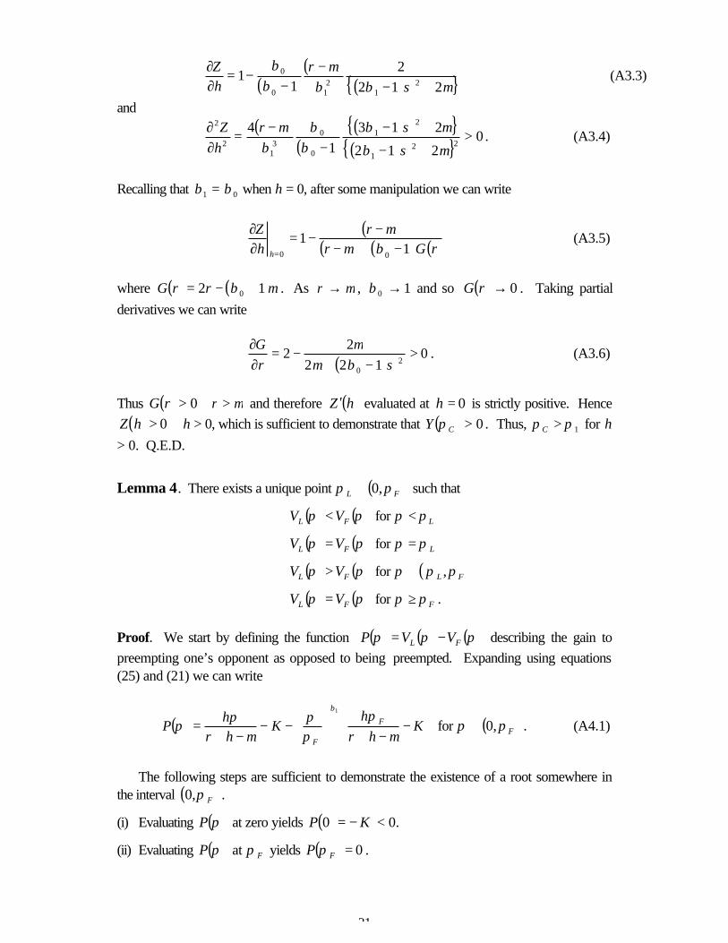
Thus ( ) 0>rG µ>∀r and therefore ( )hZ ′ evaluated at 0=h is strictly positive. Hence( ) 0>hZ ∀h > 0, which is sufficient to demonstrate that ( ) 0>CY π . Thus, 1ππ >C for h
> 0. Q.E.D.
Lemma 4. There exists a unique point ( )FL ππ ,0∈ such that
( ) ( )ππ FL VV < for Lππ <
( ) ( )ππ FL VV = for Lππ =
( ) ( )ππ FL VV > for ( )FL πππ , ∈
( ) ( )ππ FL VV = for Fππ ≥ .
Proof. We start by defining the function ( ) ( ) ( )πππ FL VVP −= describing the gain topreempting one’s opponent as opposed to being preempted. Expanding using equations(25) and (21) we can write
( )
−
−+
−−
−+= K
hrh
Khr
hP F
F µπ
ππ
µπ
πβ1
for ( )Fππ ,0∈ . (A4.1)
The following steps are sufficient to demonstrate the existence of a root somewhere inthe interval ( )Fπ ,0 .
(i) Evaluating ( )πP at zero yields ( ) KP 0 −= < 0.
(ii) Evaluating ( )πP at Fπ yields ( ) 0=FP π .

32
(iii) Evaluating the derivative ( )πP′ at Fπ it can be shown that
( ) ( ) ( ) 02 sgn sgn <
++−+
−=
Khrhrhrh
ddP
F µππ. (A4.2)
Thus, ( )πP must have at least one root in the interval (0, Fπ ).Uniqueness of the root Lπ and the validity of the two inequalities can be proven by
demonstrating strict concavity of ( )πP over ( )Fπ ,0 . By differentiation we can derive
( ) ( ) 211
11 1 −−
−
−+−−=′′ ββ π
µπ
πββπ Khr
hP F
F < 0 for π > 0. (A4.3)
Thus the root is unique, with ( ) 0<πP for ( )Lππ ,0∈ and ( ) 0>πP for( )FL πππ ,∈ .
The final equality is demonstrated by considering the follower’s optimal behaviourover the range [ )∞ , Fπ . This interval is the follower’s stopping region over which itsbest response to investment by the leader is to invest at once. Thus, the values of theleader and follower are equal over this range. Q.E.D.
Lemma 5.
(a) Sπ exists and is unique whenever ( ) ( )ππ LC VV ≥ ( )Cππ ,0∈∀ .
(b) [ ]CS ππ , forms a connected set such that ( ) ( )πππ LJJ VV ≥ ; ( )Jππ ,0∈∀ ,[ ]CSJ πππ , ∈ .
Proof.
(a) To demonstrate existence we start by showing that ( ) ( )πππ CCJ VV = ; . With somesimplification, the expressions for JV and Cπ yield
( ) ( ) ( )πππβµ
πππ ββ
β
CCC
CJ VBhr
hV ==
−+=
−00
0
0
1
2 ; . (A5.1)
It then follows from the premise that there exists at least one ( ]CJ ππ ,0∈ such that( ) ( ) ( ] ,0 ; JLJJ VV πππππ ∈∀≥ : at the very least Cπ itself satisfies this condition.
Sπ is then defined to be the smallest element of the set of joint investment pointssatisfying the condition.
With Sπ defined as the lowest joint investment point such that the two functions( )πLV and ( )SJV ππ ; just touch one another, a sufficient condition for uniqueness of
Sπ is that ( )JJV ππ ; is strictly increasing in Jπ for ( )CJ ππ ,0∈ . We derive

33
( ) ( )( ) 0
21 00 1
00 >
−+
−−=∂∂ +− ββ ππ
µπ
ββπ J
J
J
J
rhh
KV
for ( )CJ ππ ,0∈ .
(A5.2)Thus, for any CJ ππ < a higher value of Jπ entails a strictly higher value of JV at anygiven value of π .
(b) To show that [ ]CS ππ , forms a connected set satisfying the condition that( ) ( )πππ LJJ VV ≥ ; ( )Jππ ,0∈∀ , [ ]CSJ πππ , ∈ it is sufficient to show that( )JJV ππ ; is increasing in both of its arguments for all ( ]CJ ππ ,0∈ . Since JJV π∂∂
evaluated at Cπ equals zero, we can write
0≥∂∂
J
JVπ
for ( ]CJ ππ ,0∈ . (A5.3)
It can easily be seen that
( ) 010
0 >=∂∂ −βπβπ
π JJJ B
V 0>∀π . (A5.4)
Q.E.D.
The designated leader’s investment problem
The designated leader’s investment point, Dπ , is defined implicitly by
( ) ( ) 01 00011 =−
−+−+− K
hrh
B DDL β
µπ
βπββ β
where LB is as defined following expression (25). Having solved numerically for the valueof the trigger point Dπ , the option value constant DB is then defined by
−−+
=−
1
0
10
ββ
πβµ
πβ
πDL
DDD B
hrh
B .
Lemma 6. 1ππ <L for h > 0.
Proof. From rent equalisation at Lπ we know that ( ) ( )LFLL VV ππ = . Using (21) and (25)to substitute for the respective value functions at this point, and their derivatives, we canwrite
( ) ( ) ( )( )µ
βπβ
ππ−+
−+−′=′
hrhK
VVL
LLLF
111 . (A6.1)

34
From lemma 4 we know that LV crosses FV at Lπ from below and must therefore havethe steeper slope, thus ( ) ( )LFLL VV ππ ′>′ . Thus, the following upper bound for Lπ can bederived
( )( )
ML Khhr
πµ
ββ
π ≡−+
−<
11
1 . (A6.2)
Given the shape of the function ( )πY (defined by (A1.1) above) of which 1π is the root,and since 2ππ <M , it is sufficient to show that ( ) 0<MY π . It can readily be shown that
( ) ( ) ( ) ( )( ) 0
21
1
01101
<
−+
−−−−
−=
β
µµ
βββββ
πhr
rKY M for h > 0.
(A6.3)
Thus, 1πππ << ML . Q. E. D.

Figure 1: Preemptive leader-follower equilibrium
π
V
NPV - K
VL
VC
V FA
B
π π πL F C
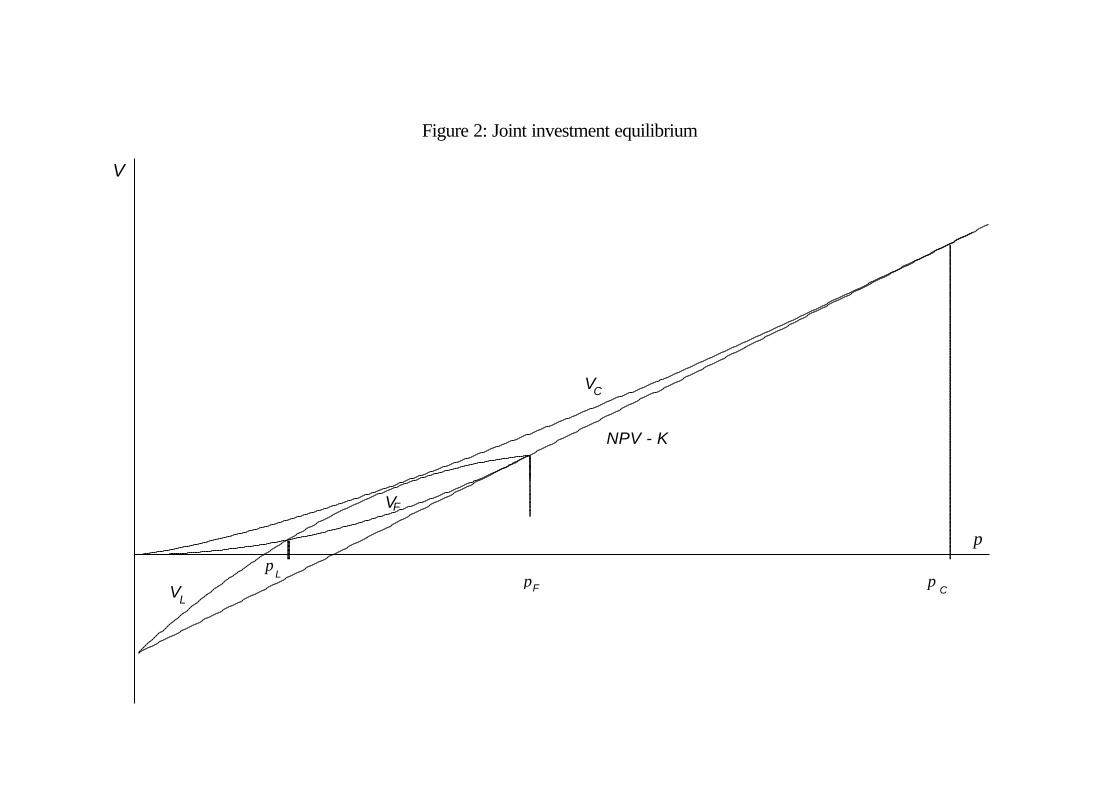
Figure 2: Joint investment equilibrium
π
V
NPV - K
VC
V L
VF
π ππ L
F C


37
References
CHOI, Jay Pil (1991), “Dynamic R&D competition under ‘hazard rate’ uncertainty,” RANDJournal of Economics, 22 (winter), 596-610.
DASGUPTA, Partha, and Joseph STIGLITZ (1980), “Uncertainty, industrial structure, andthe speed of R&D,” Bell Journal of Economics, 11, 1−28.
DIXIT, Avinash K. (1988), “A general model of R&D competition and policy,” RANDJournal of Economics, 19 (autumn), 317−326.
—— (1989), “Entry and exit decisions under uncertainty,” Journal of Political Economy,97 (June), 620-638.
—— (1991), “Irreversible investment with price ceilings,” Journal of Political Economy,99 (June), 541-557.
—— and Robert S. PINDYCK (1994), Investment Under Uncertainty, PrincetonUniversity Press.
DUTTA, Prajit K., and Aldo RUSTICHINI (1991), “A theory of stopping time games withapplications to product innovations and asset sales,” Columbia University DiscussionPaper Series no. 523.
FUDENBERG, Drew, Richard GILBERT, Joseph STIGLITZ and Jean TIROLE (1983),“Preemption, leapfrogging, and competition in patent races,” European EconomicReview, 22, 3-31.
FUDENBERG, Drew, and Jean TIROLE (1985), “Preemption and rent equalisation in theadoption of new technology,” Review of Economic Studies, 52, 383-401.
—— and —— (1986), “A theory of exit in duopoly,” Econometrica 54 (July), 943-960.
—— and —— (1991), Game Theory, MIT Press.
GHEMAWAT, Pankaj, and Barry NALEBUFF (1985), “Exit,” RAND Journal ofEconomics, 16, 184-194.
GRENADIER, Steven R. (1996), “The strategic exercise of options: Developmentcascades and overbuilding in real estate markets,” Journal of Finance, 51 (December),1653-1679.
HARRISON, J. Michael (1985), Brownian Motion and Stochastic Flow Systems, JohnWiley & Sons, New York.
KAMIEN, Morton I., and Nancy L. SCHWARTZ (1982), “Market Structure andInnovation,” Cambridge University Press, Cambridge.
KULATILAKA, Nalin, and Enrico C. PEROTTI (1998), “Strategic Growth Options,”Management Science, 44 (August), 1021-1031.
LAMBRECHT, Bart, and William PERRAUDIN (1997), “Real options and preemption,”University of Cambridge, JIMS Working paper no. 15/97.

38
LEE, Tom, and Louis L. WILDE (1980), “Market structure and innovation: Areformulation,” Quarterly Journal of Economics, 94 (March), 429−436.
LOURY, Glenn C. (1979), “Market structure and innovation,” Quarterly Journal ofEconomics, 93 (August), 395−410.
MASKIN, Eric, and Jean TIROLE (1988), “A theory of dynamic oligopoly I: Overviewand quantity competition with large fixed costs,” Econometrica, 56, 549-570.
McDONALD, Robert, and Daniel SIEGEL (1986), “The value of waiting to invest,”Quarterly Journal of Economics, 101 (November), 707-728.
PINDYCK, Robert S. (1988), “Irreversible investment, capacity choice, and the value ofthe firm,” American Economic Review, 79 (December), 969-985.
REINGANUM, Jennifer (1981), “On the diffusion of new technology: A game-theoreticapproach,” Review of Economic Studies, 153, 395-406.
—— (1983), “Uncertain innovation and the persistence of monopoly,” AmericanEconomic Review, 73 (September), 741-748.
SMETS, Frank (1991), “Exporting versus foreign direct investment: The effect ofuncertainty, irreversibilities and strategic interactions,” Working Paper, Yale University.

39
1 This value could be interpreted as the expected NPV of profits in the relevant product
market or, if further sunk costs are required, might itself be the value of the option to investin this market, making investment in the research stage a compound option problem.
2 The restriction that µ < r, commonly found in real options models, is necessary to ensurethat there is a strictly positive opportunity cost to holding the option, so that it will not be heldindefinitely. A large negative drift term would, ceteris paribus, encourage earlierinvestment to raise the probability of winning the prize before its value declines significantly,counteracting the option effects in the model. To avoid such an outcome we make theassumption that µ is non-negative. Since the model is concerned with the effects ofuncertainty, not expected trends, the conclusions from the analysis are unaffected by thisassumption.
3 Thus the cost of R&D is fixed, or contractual in the terminology of Kamien and Schwartz(1982).
4 To be precise, the statement that a firm invests at a trigger point π* means that the firminvests at the time when the stochastic process π first hits the value π*, approaching thislevel from below.
5 For further details see Fudenberg and Tirole (1985), section 4.6 If smooth-pasting were violated and instead a kink arose at Uπ , a deviation from the
supposedly optimal policy would raise the firm’s expected payoff. By delaying for a smallinterval of time after the stochastic process first reached Uπ , the next step dπ could beobserved. If the kink were convex, the firm would obtain a higher expected payoff byentering if and only if π has moved (strictly) above Uπ , since an average of points on eitherside of the kink give it a higher expected value than the kink itself. If the kink wereconcave, on the other hand, second order conditions would be violated. Continuation alongthe initial value function would yield a higher payoff than switching to the alternativefunction and switching at Uπ could not be optimal. More detailed explanation of thiscondition can be found in appendix C of chapter four in Dixit and Pindyck (1994). Note thatthis condition applies for all diffusion processes, not just a geometric Brownian motion suchas (1).
7 It is implicitly assumed that side payments may be used to ensure that neither firm has anincentive to deviate; alternatively, the two firms may be separate research units controlledby an integrated firm.
8 Smooth-pasting ensures that the first derivative of FLV + is continuous at 1π .9 An analogous effect is found in the duopoly models of Smets (1991) and Grenadier (1996).
The second, option value effect of rival investment is absent from these models, however.10 With K adjusted appropriately so that the project’s expected value remains constant.11 With µ adjusted in line so that the opportunity cost µδ −= r remains constant.12 Given that this proportion is determined largely by the duration of the patent and the degree
of monopoly power conveyed by the patent grant, this would not seem to be anunreasonable assumption.
13 All values and trigger points are scaled up by the same proportion, leaving the optimal timingof investment unchanged.