strain assessment in echo€¦ · · 2011-09-06strain assessment in echo joe m. moody, jr, md...
TRANSCRIPT

Strain Assessment in Echo
Joe M. Moody, Jr, MD
UTHSCSA and STVHCS
2010
Acknowledging many illustrations from Weyman’s text and others.
Echo-Doppler Basic Principles
• Background:
– Ultrasound physics (resolution,
attenuation)
– Doppler ultrasound (PW, CW, Color)
– Ventricular Strain
• Echo measurement of Strain

Ultrasound
physics
• Sound - waves of compression and rarefaction propagated through a medium
• Ultrasound - sound frequency above 20kHz
• Cardiac ultrasound - 1 - 20 mHz
• Intensity - watts/cm2 (joule/sec/cm2)

Sound
Wave
Diagram
Otto CM. Textbook of Clinical Echocardiography. 2000.
Wavelength times frequency equals propagation velocity
c=λ*f, and c=1540 m/s, so λ (mm)= 1.54/f (MHz)
λ for 2 MHz is 0.75mm
λ for 4 MHz is 0.38mm
c=λ*f

Piezoelectricity
• Mechanical stress applied to a crystal causes electrical charges bound in the crystal to shift to the surface where they can be measured as a voltage
• Electric current applied to a crystal changes the crystal shape, alternating current can cause vibration of crystal, producing sound wave
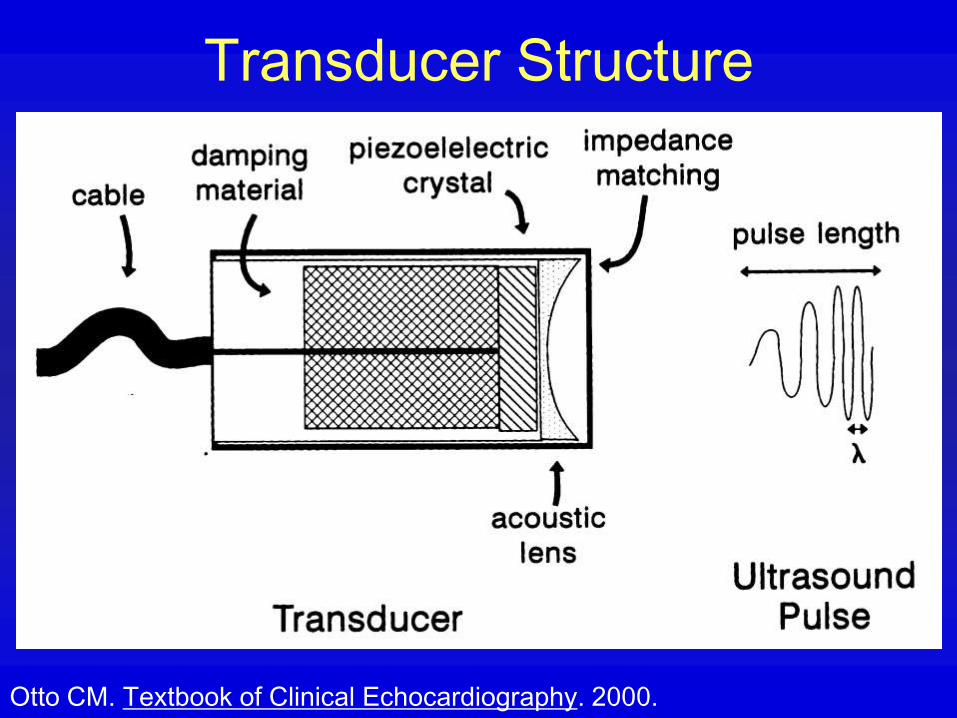
Transducer Structure
Otto CM. Textbook of Clinical Echocardiography. 2000.

Wavelength versus Penetration
Otto CM. Textbook of Clinical Echocardiography. 2000.
Coronary IVUS
Retinal

Echo Transducer
• Definitions of fields of transducer
performance

Echo
Transducer• Single crystal
• Effect of crystal diameter and frequency on near field and far field
• Larger diameter and higher frequency give longer near field and less divergent far field

Transducer Beam Zones
Otto CM. Textbook of Clinical Echocardiography. 2000.

Echo Transducer
• Effect of
focal length
and focusing
on near field
and far field

Graph: Transducer Beam Zones
Otto CM. Textbook of Clinical Echocardiography. 2000.
Solid line: length of near zone
Dashed line: divergence angle

Side Lobe Artifacts

Side Lobe Artifacts

Echo Transducer Lateral Variation

Side Lobe
Artifact in Single
Crystal
Transducer
Otto CM. Textbook of Clinical Echocardiography. 2000.
Position of side lobes at
locations where the distances
from each edge of the crystal
face differ by one wavelength

Grating Lobe
Artifact in
Phased-
Array
Transducer
Otto CM. Textbook of Clinical Echocardiography. 2000.
Position of grating lobes is
determined by spacing
between centers of
independent crystal elements
in the transducer.
S=spacing between elements
F=focal length
λ=wavelength

Echo Transducer Axial
Variation

Phased Array Echo
Transducer

Phased Array Echo
Transducer
• Effect of electronic focus

Destiny of Sound Wave
Otto CM. Textbook of Clinical Echocardiography. 2000.

Velocity of Sound in Air and
Various Tissues
• Air 330 m/s
• Fat 1450 m/s
• Water 1480 m/s
• Soft tissue 1540 m/s
• Kidney 1560 m/s
• Blood 1570 m/s
• Muscle 1580 m/s
• Bone 4080 m/s
Feigenbaum, 6th ed, 2005, p. 13.
Clinically, use
1500 m/s

Velocity and Time
Relation in
Echocardiography
• Distance = rate * time
• Time = distance/rate
• Distance/rate (for 15 cm)= – 0.15m/1500m/sec =
– .0001 sec, or 1/10,000 sec for one way trip
– .0002 sec or 2/10,000 sec for 2 way trip
– .0003 or 3/10,000 sec for 2 way trip of 20 cm

Display of Echo Signal
A = amplitude B = brightness M = motion

Echo Interfaces
• Velocity of sound in a medium depends on density (denser is faster) and elasticity of the medium
• Human tissue - 1540 m/sec, faster in bone
• Acoustic mismatch or change in acoustic impedance of an interface causes a reflection
• Interface perpendicular to beam is strongest

Echo Reflection
• Specular reflection - reflector is large
and smooth relative to ultrasound
wavelength - responsible for the echo
images, angle of incidence is important
• Scattered reflection - reflector is small
and rough relative to ultrasound
wavelength - responsible for some
images and critical for Doppler

Echo Resolution and Attenuation
• Axial resolution - better with higher frequency and fewer cycles/pulse (packet size) 3.5MHz=0.43mm wavelength
• Lateral resolution - varies with transducer size, shape, frequency, and focusing
• Attenuation - worse with high frequency
• Attenuation - half-value layer (35cm in blood, 3.6 cm in muscle)

Echo Attenuation – Half-power
Distance
• Water 380 cm
• Blood 15 cm
• Soft tissue (except muscle) 1-5 cm
• Muscle 0.6-1 cm
• Bone 0.2-0.7 cm
• Air 0.08 cm
• Lung 0.05 cm
Feigenbaum, 6th ed, 2005, p. 14.

Axial
Resolution
• Better with:
– high
frequency
– short packet
length

Time Constraint in Echo-Doppler
• 1540 m/sec in tissue
• 20 cm depth is 40 cm round trip
• 3850 round trips/sec (M-mode)
• 150 round trips for one image
• 25 images/sec
• Trade-off: temporal resolution, spatial resolution (line density) and depth

Time
Constraint
in Echo-
Doppler
• 1540 m/sec in tissue, 20 cm depth is 40 cm round trip, 3850 round trips/sec (M-mode), 150 round trips for one image, 25 images/sec
• Trade-off: temporal resolution, spatial resolution (line density) and depth
• In the “Res” mode, there is improved temporal resolution

Time Constraint in Echo-Doppler
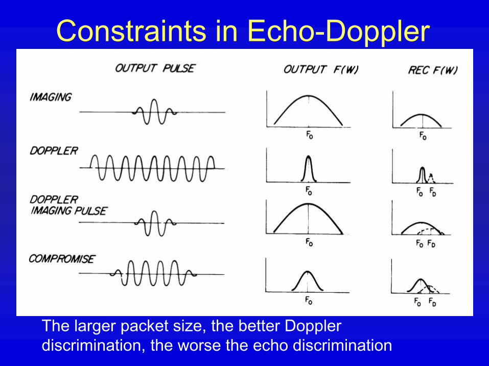
Constraints in Echo-Doppler
The larger packet size, the better Doppler
discrimination, the worse the echo discrimination

Time Constraint in Echo-Doppler
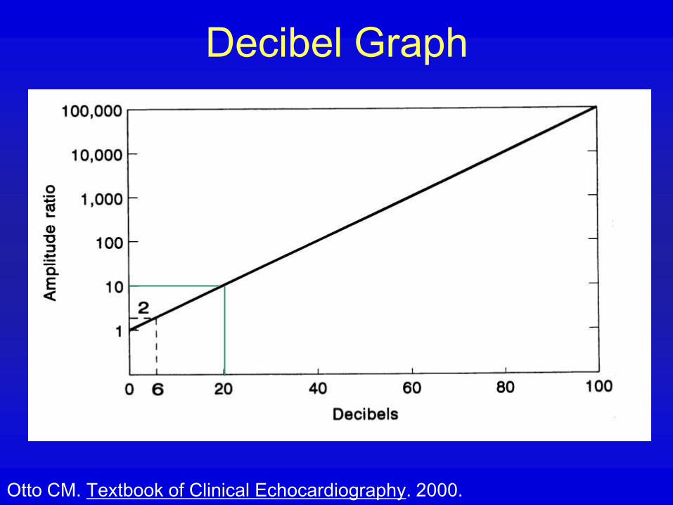
Decibel Graph
Otto CM. Textbook of Clinical Echocardiography. 2000.

Artifact From Scatter
Otto CM. Textbook of Clinical Echocardiography. 2000.

Artifact
From
Scatter
Otto CM. Textbook of Clinical Echocardiography. 2000.

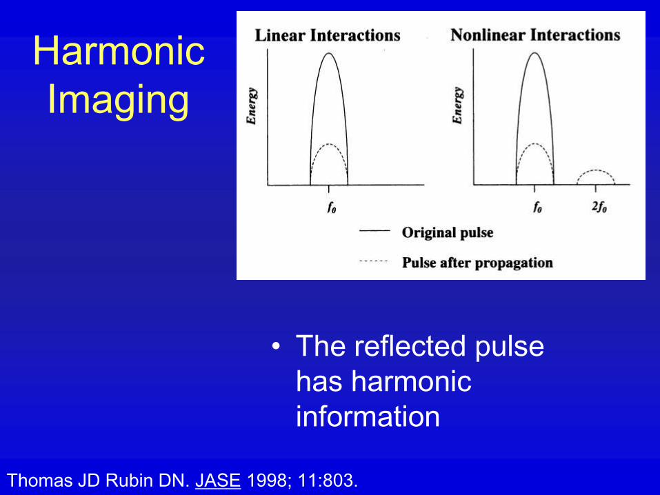
Breakthrough:
Harmonic Imaging
• Since about 1997 with the introduction of harmonic imaging, there has been a dramatic improvement in image quality
• Today, essentially all images are obtained with harmonic imaging
• Sound travels a little faster at the peak of the sound wave (more compressed) than the trough, so with each subsequent waveform a small amount of harmonic is generated (1962), similar to the breaking of the crest of a wave at the beach
Thomas JD Rubin DN. JASE 1998; 11:803.

2 Types of Harmonic Imaging
• Harmonic energy in reflection can occur
with echo-contrast agents which
resonate with ultrasound stimulation
and produce harmonic emission
• Harmonic energy in transmission occurs
due to the compressibility of the tissue
Thomas JD Rubin DN. JASE 1998; 11:803.

Harmonic Imaging
Classical ultrasound theory:
• Energy propagation is linear
• Different frequencies travel at the same speed in the same medium
• New frequencies should not appear
• Attenuation only reduces amplitude
Harmonics:
• Some objects in the path of
the beam may resonate
and emit higher
frequencies
• Transmission of ultrasound
through a compressible
medium yields harmonics
• Signal grows with distance
• Signal generation is
nonlinear
• Reduced backscatter
Thomas JD Rubin DN. JASE 1998; 11:803.
Harmonic
Imaging
• The reflected pulse
has harmonic
information
Thomas JD Rubin DN. JASE 1998; 11:803.
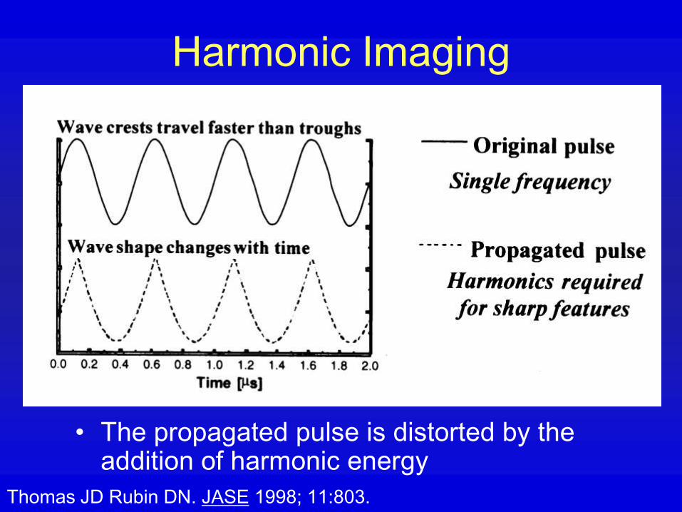
Harmonic Imaging
• The propagated pulse is distorted by the addition of harmonic energy
Thomas JD Rubin DN. JASE 1998; 11:803.

Harmonic Imaging
• The harmonic energy increases with depth
Thomas JD Rubin DN. JASE 1998; 11:803.

Harmonic Imaging
• Strength of harmonics increases as square of source energy, so weak reflections produce poor harmonics
Thomas JD Rubin DN. JASE 1998; 11:803.

Harmonic Imaging
• Boosting of harmonic information is required
Thomas JD Rubin DN. JASE 1998; 11:803.

Harmonic
Imaging
• Narrow band pulse is smoother in initiation and termination
Thomas JD Rubin DN. JASE 1998; 11:803.

Harmonic
Imaging
• The square pulse (wide band) has significant energy at many frequencies, including at the harmonic frequency
• In contrast, the smooth pulse (narrow band) has almost no energy at the harmonic frequency
Thomas JD Rubin DN. JASE 1998; 11:803.

Harmonic Imaging
• Narrow band pulse allows filtered signal to be essentially free of fundamental frequency reflection
Thomas JD Rubin DN. JASE 1998; 11:803.

New Instrumentation: High
PRF Equipment
• The classical time constraints explained
earlier are rendered nonconstraining by
the process of multiple simultaneous
scan line analysis
• I don’t understand it

Doppler Cardiography
• Primary source of ultrasonic reflection -
RBC
• Scattered reflector
• Motion with respect to transducer
causes shift in frequency of sound
wave, the measurement of which is
fundamental to the Doppler signal

Doppler Shift
Otto CM. Textbook of Clinical Echocardiography. 2000.
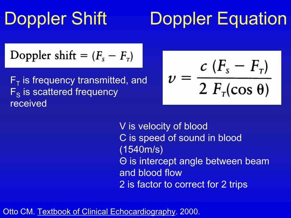
Doppler Shift Doppler Equation
Otto CM. Textbook of Clinical Echocardiography. 2000.
FT is frequency transmitted, and
FS is scattered frequency
received
V is velocity of blood
C is speed of sound in blood
(1540m/s)
Θ is intercept angle between beam
and blood flow
2 is factor to correct for 2 trips
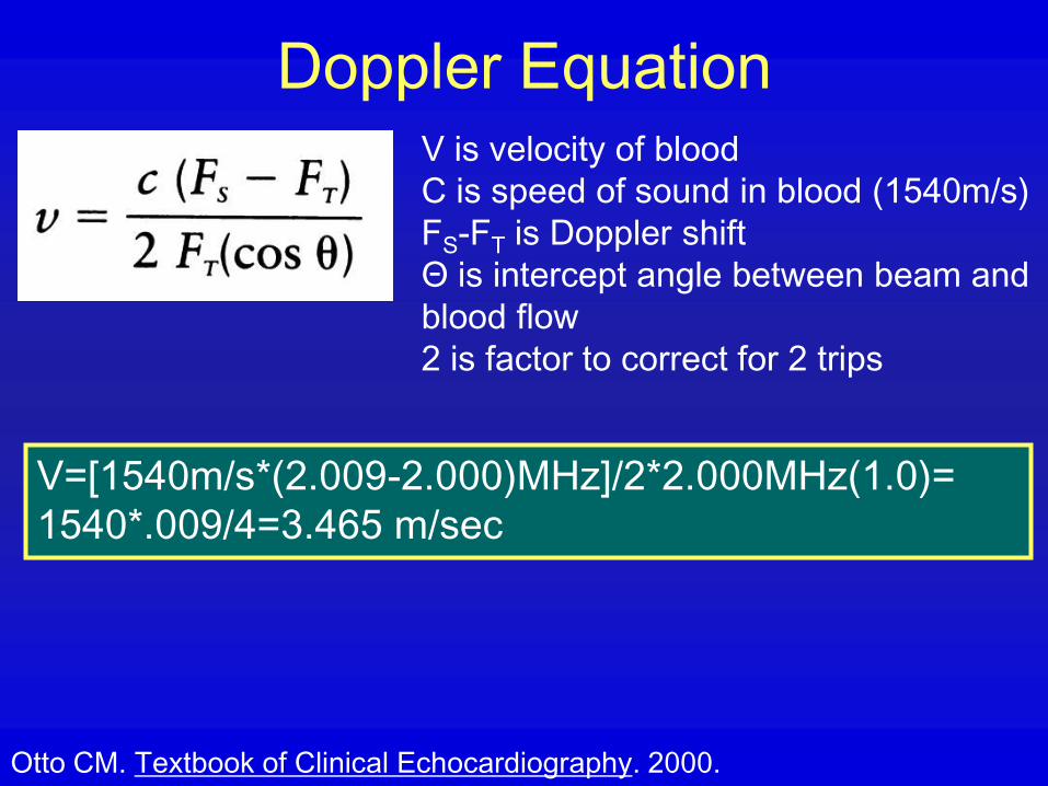
Doppler Equation
Otto CM. Textbook of Clinical Echocardiography. 2000.
V is velocity of blood
C is speed of sound in blood (1540m/s)
FS-FT is Doppler shift
Θ is intercept angle between beam and
blood flow
2 is factor to correct for 2 trips
V=[1540m/s*(2.009-2.000)MHz]/2*2.000MHz(1.0)=
1540*.009/4=3.465 m/sec
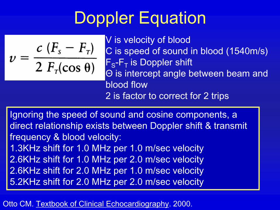
Doppler Equation
Otto CM. Textbook of Clinical Echocardiography. 2000.
V is velocity of blood
C is speed of sound in blood (1540m/s)
FS-FT is Doppler shift
Θ is intercept angle between beam and
blood flow
2 is factor to correct for 2 trips
Ignoring the speed of sound and cosine components, a
direct relationship exists between Doppler shift & transmit
frequency & blood velocity:
1.3KHz shift for 1.0 MHz per 1.0 m/sec velocity
2.6KHz shift for 1.0 MHz per 2.0 m/sec velocity
2.6KHz shift for 2.0 MHz per 1.0 m/sec velocity
5.2KHz shift for 2.0 MHz per 2.0 m/sec velocity

Timing in Pulsed Doppler: The PRF
Otto CM. Textbook of Clinical Echocardiography. 2000.
Pulse Cycle Consists of Three periods:
•Transmission (duration affects velocity resolution)
•Travel time (duration determines depth)
•Reception (duration determines sample volume)
PRF is
mainly
limited by
depth in
Pulsed
Doppler
Ultrasound

Timing in Pulsed Doppler
Otto CM. Textbook of Clinical Echocardiography. 2000.
A waveform must be sampled at least twice in each cycle for
accurate determination of wavelength.
Therefore, the maximum detectable frequency shift (the
Nyquist Limit) is one-half the PRF. But the maximal
detectable velocity depends on the equation.
A: Sampling at three
times the cycle rate,
apparent direction is
clockwise
B: With sampling at less
than twice the cycle rate,
apparent direction is
counterclockwise

Nyquist Limit
• The maximum detectable frequency
shift (the Nyquist Limit) is one-half
the PRF. But the maximal
detectable velocity depends on the
equation.
Let’s say the PRF is 5000.
Nyquist limit= (2500Hz or 2.5KHz=.0025MHz)=
[1540m/s*(PRF/2)MHz]/2*2.000MHz(1.0)=
[1540m/s*(0.0025)MHz]/2*2.000MHz(1.0)=
1540*.00025/4=0.9625 m/sec= 96cm/sec

High PRF Doppler
Otto CM. Textbook of Clinical Echocardiography. 2000.

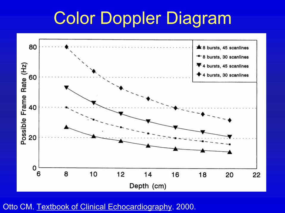
Color Doppler Diagram
Otto CM. Textbook of Clinical Echocardiography. 2000.

Color Doppler Diagram
Otto CM. Textbook of Clinical Echocardiography. 2000.
Color Doppler Diagram
Otto CM. Textbook of Clinical Echocardiography. 2000.
Type of Doppler Signal
• Pulsed wave Doppler
• Continuous wave Doppler
• Color flow Doppler (a form of pulsed
wave Doppler)
• (High pulse repetition frequency pulsed
wave Doppler is intermediate between
pulsed and continuous wave)

Types of Doppler Signal
Pulsed wave Continuous
wave
High PRF
Aliasing Yes No Yes, better
High velocity No Yes Yes
Range specific Yes No Some
ambiguity
Laminar
Resolution
Yes No Yes, somewhat

Principles of Imaging
• Reducing scan angle can increase line
density
• Side lobe artifacts can be generated by
the transducer
• Signal processing can alter relationship
between strength of received signal and
display strength

Principles of Imaging - 2
• Persistence of image on screen
smoothes discontinuities (temporal
image processing)
• Signal processing is complex
• Connection with video monitor is not
trivial, and can result in signal loss

Principles of Imaging• Persistenc
e of image on screen smoothes discontinuities (temporal image processing)
• Signal processing is complex
• Connection with video monitor is not trivial, and can result in signal loss
Big Otto, 1997

Principles of Imaging -
Contrast
• Contrast enhancement with specular
reflectors
– air microbubbles
– protein microparticles
• Contrast location
– bloodstream
– myocardial (experimental)

Imaging Advances
• Imaging traditionally looks for the
frequency transmitted
– Human tissue naturally causes increase in
frequency of returned signal, and can be
imaged at twice the transmitted frequency
– Native tissue harmonic imaging
• Tissue characterization

Echo Artifacts
• Incorrect persistence on screen - bright
object may last into subsequent frames
• Point spread function in far field
• Internal reverberations, projected at
twice the real distance
• Reverberations from highly reflective
interface may be a series of echoes
• Shadowing behind a strong reflector

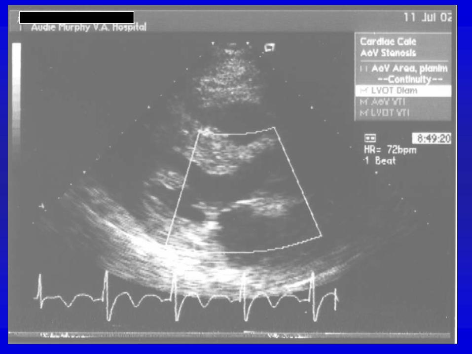
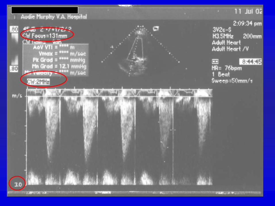
Uses of Doppler Information
• Analysis of velocity
• Analysis of turbulence
• Analysis of valve area
– MV - pressure half time
– Continuity Equation
• Analysis of pressure difference,
instantaneous or mean

Blood Flow
• The original and still most commonly used source of Doppler information
• Flow is generally either laminar or turbulent depending on whether Reynold’s number is exceeded (about 5,000-10,000)
• Reynolds: 2RVp/n where R=radius, V=velocity, p=density, n=viscosity
• Flow is usually at least somewhat pulsatile
Murgo, JP. J Am Coll Cardiol. 1998;32:1596-1602, Weyman AE text 1994, p. 191.

Doppler Pressure Gradient
)()(2/1
2
1
2
1
2
2
vR
sdtd
vdvvP
Convective acceleration
plus flow acceleration plus
viscous forces
Weyman AE Text, 2nd ed. 1994, p. 195.

Bernoulli Equation
)()(2/1
2
1
2
1
2
2
vR
sdtd
vdvvP
1. Convective acceleration – Velocity squared
Pressure energy kinetic energy
2. Flow acceleration – Derivative of velocity
Energy to impart momentum
3. Viscous forces – Velocity
Energy losses from friction between neighboring fluid
elements, more with turbulence
3.972 4
1. 2.3.

Bernoulli Equation
)()(2/1
2
1
2
1
2
2
vR
sdtd
vdvvP
1. Convective acceleration
2. Flow acceleration
3. Viscous forces
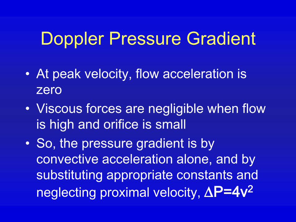
Doppler Pressure Gradient
• At peak velocity, flow acceleration is
zero
• Viscous forces are negligible when flow
is high and orifice is small
• So, the pressure gradient is by
convective acceleration alone, and by
substituting appropriate constants and
neglecting proximal velocity, P=4v2

Pulsed Doppler Limit
• Nyquist limit: Aliasing occurs when the
frequency of the Doppler shift exceeds
1/2 the PRF
– Doppler shift is proportional to transducer
frequency
– More with greater depth of sample volume
– Decrease effect by shift of baseline
– Decrease effect by increasing angle of
signal

Doppler Artifacts
• Aliasing (also range ambiguity)
• Mirroring - when Doppler shift is displayed as equal frequency and opposite direction (solve by decreasing gain)
• Display of external audible noise as Doppler
• Signal loss by data sharing
• Beam width artifact

Color Doppler Artifacts
• Color aliasing
• Reverberations
• Effects of wall shadowing
– usual suppression
– suppression by strong echo signal
• Effects of flow angle in the scan plane

Color Doppler M-Mode
From GE website

Doppler Advances
• Contrast Doppler for myocardial
perfusion
– Intracoronary
– Intravenous (perfluorocarbons)
• Doppler analysis of tissue
– Wall motion
– Strain
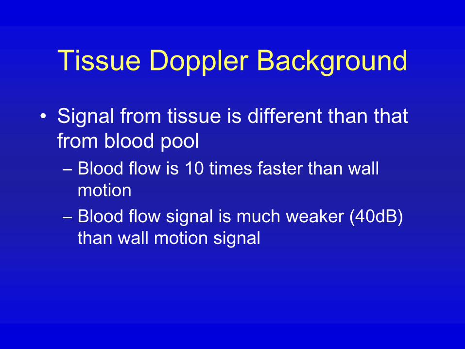
Tissue Doppler Background
• Signal from tissue is different than that
from blood pool
– Blood flow is 10 times faster than wall
motion
– Blood flow signal is much weaker (40dB)
than wall motion signal

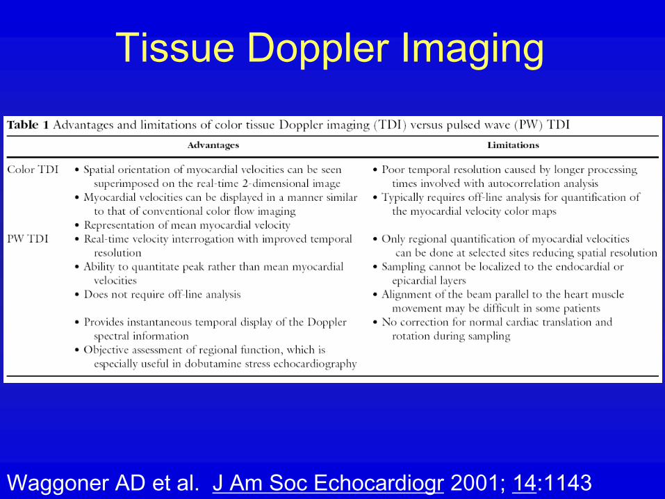
Tissue Doppler Imaging
Techniques
• High pass wall filter is disabled
• Gain amplification for low velocity or
reduction for myocardium
• Expanded scale (peak less than 25
cm/s)
• Small (2 mm) sample volume (“gate”)
Waggoner AD et al.
J Am Soc Echocardiogr 2001; 14:1143

Tissue
Doppler
Imaging
• Gate: lateral LV
base in A4C
• V1 – systolic
• V2 – early
diastolic
• V – late diastolic
Excessive gain
-0.12 -0.06
0.07
Waggoner AD et al.
J Am Soc Echocardiogr 2001; 14:1143

Tissue
Doppler
Imaging
• Gate:
midventricular
septum in A4C
• Large gate
(20mm) gives
inadequate
recording
Large gate
Tachycardia – merged flowsWaggoner AD et al.
J Am Soc Echocardiogr 2001;
14:1143
Tissue Doppler Imaging
Waggoner AD et al. J Am Soc Echocardiogr 2001; 14:1143

Tissue Doppler Imaging
Waggoner AD et al. J Am Soc Echocardiogr 2001; 14:1143

Normal Tissue Doppler Imaging
Waggoner AD et al. J Am Soc Echocardiogr 2001; 14:1143
A4C
A2C

Tissue
Doppler
Imaging
Waggoner AD et al. J Am Soc Echocardiogr 2001; 14:1143
• Normal tissue
Doppler signal
from basal lateral
wall in A4C

Tissue
Doppler
Imaging
Waggoner AD et al. J Am Soc Echocardiogr 2001; 14:1143
• Patient with prior
anteroseptal MI
• Top: septal base
• Bottom: lateral
base
• V1 systolic velocity
• V2 diastolic velocity
Tissue
Doppler
Imaging
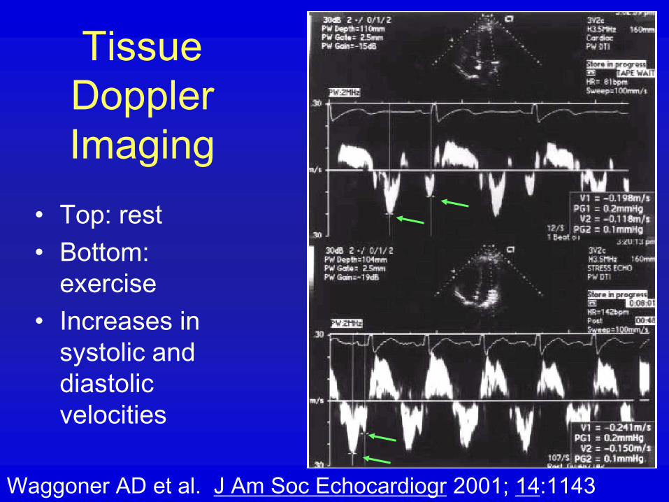
Waggoner AD et al. J Am Soc Echocardiogr 2001; 14:1143
• Top: rest
• Bottom:
exercise
• Increases in
systolic and
diastolic
velocities

Tissue
Doppler
Imaging
Waggoner AD et al. J Am Soc Echocardiogr 2001; 14:1143
• Htn and LVH
• Pseudonormalized
LVIT pattern
• Abnormal TDI of
lateral base with
decreased early
diastolic velocity and
normal late diastolic
velocityEm= 6
Nl = 13.3±3.3
LVIT
Am= 13

Color Tissue Doppler Imaging
Trambaiolo P et al. JASE 2001; 14:85
b=regional
isovolumic
contraction time
c=regional
isovolumic relaxation
time
s=systole
E=rapid filling
A=atrial contraction

Background: LV Stress
• Ventricular performance – pressure and
volume
• Myocardial performance – stress (pressure
and radius and also wall thickness)
– Laplace relation: σ = (P*r)/2h, where sigma is wall
stress, P is pressure, r is radius and h is wall
thickness
• Components of stress: circumferential,
meridional, and radial

Carroll JD and Hess OM. Ch 20,
“Assessment of Normal and
Abnormal Cardiac Function”
Braunwald’s Heart Disease, 7th ed.
2004.
Components of stress:
circumferential,
meridional, and
Radial
Stress: (P*r)/2h

LV Strain Background• LV strain is caused by stress – change in
pressure or force on the LV wall
• LV strain is a deformation of the wall shape
(length) related to stress
• LV strain can be due to shortening and
contractility (active) or relaxation and filling
• Normally LV strain in systole is negative
(shortening), and in diastole is positive
• Strain rate is just the rate of change in
dimension

Strain Rate Imaging
Hoffmann R et al. JACC 2002;39:443
Septal wall
More yellow in
the mid-anterior
segment
indicates
increase in
contractility,
indicating
viability

Tissue Doppler Applications
• Not widely used
• Diastolic function
• Regional systolic function
• Strain measurement using tissue
Doppler displayed as tissue velocity
imaging in color
For images to view and clips to see, try GE Medical Systems website
http://www.gemedicalsystems.com/rad/us/products/vivid_7/msuvivid7img.html