NAVAL POSTGRADUATE SCHOOLMonterey, California

THESISSTORE SEPARATION

METHODOLOGY ANALYSIS

byDarcy Michael Hansen

September, 1991

Thesis Advisor:Co-Advisor:

Prof. Oscar BiblarzProf. Louis Schmidt

Approved for public release; distribution is unlimited

T260851

Unclassified

security classification of this page

REPORT DOCUMENTATION PAGE

la REPORT SECURITY CLASSIFICATION

Unclassified

lb RESTRICTIVE MARKINGS

2a SECURITY CLASSIFICATION AUTHORITY

2b DECLASSlFiCATlON/DOWNGRADING SCHEDULE

3 DISTRIBUTION/AVAILABILITY OF REPORT

Approved for public release, distribution is unlimited

4 PERFORMING ORGANIZATION REPORT NUMBER(S) 5 MONITORING ORGANIZATION REPORT NUMBER(S)

6a NAME OF PERFORMING ORGANIZATION

Naval Postgraduate School

6b OFFICE SYMBOL(If applicable)

31

7a NAME OF MONITORING ORGANIZATION

Naval Postgraduate School

6c ADDRESS (City, State, and ZIP Code)

Monterey, CA 93943-5000

7b ADDRESS (City, State, and ZIP Code)

Monterey, CA 93943 5000

8a NAME OF FUNDING/SPONSORINGORGANIZATION

8b OFFICE SYMBOL(If applicable)

9 PROCUREMENT INSTRUMENT IDENTIFICATION NUMBER

8c ADDRESS (City. State, and ZIP Code) 10 SOURCE OF FUNDING NUMBERS

Program t lenient No Hroiea No Work unit Accev>ion

Number

1 1 TITLE (Include Security Classification)

Store Separation Methodology Analysis

12 PERSONAL AUTHOR(S) Hansen, Darcy M.

13a TYPE OF REPORT

Master's Thesis

13b TIME COVERED

From To

14 DATE OF REPORT (year, month, day)

1991, September

15 PAGE COUNT81

16 SUPPLEMENTARY NOTATION

The views expressed in this thesis are those of the author and do not reflect the official policy or position of the Department of Defense or the U.S.

Government.

17 COSATI CODES

FIELD GROUP SUBGROUP

18 SUBJECT TERMS (continue on reverse if necessary and identify by block number)

separation, store, trajectory

1 9 ABSTRACT (continue on reverse if necessary and identify by block number)

Various computational methods and operational computer codes used to predict the aerodynamic coefficients and separation trajectories of

aircraft stores are examined. The semi-empirical aeroprediction code Missile DATCOM is used to obtain the coefficients of a modeled store. These

coefficients, together with the modeled ejection forces, are used in free-stream state-space equations of motion to predict the store trajectory. The

results are compared with the Nielson Engineering and Research (NEAR) store separation code which provides accurate trajectory profiles, for

speeds below the subsonic Macb critical speed, by use of a vortex-lattice and panel method. Modification of the Missile DATCOM aerodynamic

coefficients provides single-point state-space prediction of the store pitch trajectory to within 30% of the NEAR code values. Store trajectories

were restricted to the first 0.2 seconds of free-flight.

20 DISTRIBUTION/AVAILABILITY OF ABSTRACT

F&JNCLASSIFIEO/UNLlMlTED j SAME AS REPORT J OTIC USERS

22a NAME OF RESPONSIBLE INDIVIDUAL

Prof. Oscar Biblarz

21 ABSTRACT SECURITY CLASSIFICATION

Unclassified

22b TELEPHONE (Include Area code)

(408)646-3096

22c OFFICE SYMBOLAA/BI

DD FORM 1473, 84 MAR 83 APR edition may be used until exhausted

All other editions are obsolete

SECURITY CLASSIFICATION OF THIS PAGE

Unclassified

Approved for public release; distribution is unlimited.

Store Separation

Methodology Analysis

by

Darcy M. Hansen

B.S., Arizona State University, 1983

Submitted in partial fulfillment

of the requirements for the degree of

MASTER OF SCIENCE IN AERONAUTICAL ENGINEERING

from the

NAVAL POSTGRADUATE SCHOOLSeptember 1991

n

ABSTRACT

Various computational methods and operational computer codes used to predict the

aerodynamic coefficients and separation trajectories of aircraft stores are examined. The

semi-empirical aeroprediction code Missile DATCOM is used to obtain the coefficients

of a modeled store. These coefficients, together with the modeled ejection forces, are

used in free-stream state-space equations of motion to predict the store trajectory. The

results are compared with the Nielson Engineering and Research (NEAR) store separation

code which provides accurate trajectory profiles, for speeds below the critical speed, by

use of a vortex-lattice and panel method. Modification of the Missile DATCOM

aerodynamic coefficients provides single-point state-space prediction of the store pitch

trajectory within 30% of the NEAR code results. Store trajectories were restricted to the

first 0.2 seconds of free flight.

iii

I

TABLE OF CONTENTS

I

.

STORE SEPARATION INTRODUCTION 1

A. BACKGROUND 1

B. MATHEMATICAL MODELING 2

C. METHODOLOGY 3

II. EJECTION FORCES AND MOMENTS 5

A. EJECTOR CHARACTERISTICS 5

B. FORCES 8

1

.

Theory 8

2

.

Example 8

C. MOMENTS 9

1

.

Theory 9

2

.

Example 9

D. PRELIMINARY OBSERVATION 10

III. AERODYNAMIC CALCULATION 11

A. THEORY 11

1. Longitudinal Equations 12

2. Lateral Equations 13

3. State Variable Representation 14

B. MISDATCOM 15

1 . Theory 15

IV

2. Procedure 17

C. AERODYNAMIC CALCULATION 20

1. Longitudinal 20

2. Lateral 23

D. PARAMETER VARIATION 23

E. PRELIMINARY OBSERVATION 24

IV. "NEAR" PROGRAM 25

A. BACKGROUND 25

B. THEORY 2 6

1. Source Program 26

2

.

Trajectory Program 27

3. Shape Modeling 28

C. PROCEDURE 31

1

.

Source Program 31

2

.

Trajectory Program 35

V. RESULTS AND COMPARISONS 40

A. EJECTOR FORCES AND MOMENTS 4

1. Vertical Velocity 40

2. Pitch Rate Q 40

B. TRAJECTORY COMPARISON 40

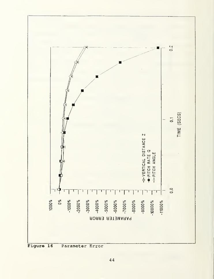
1. Vertical Separation Z 41

2. Pitch Angle 41

3. Pitch Rate 45

4. Vertical Velocity 45

v

C. AUGMENTED AEROPREDICTION 45

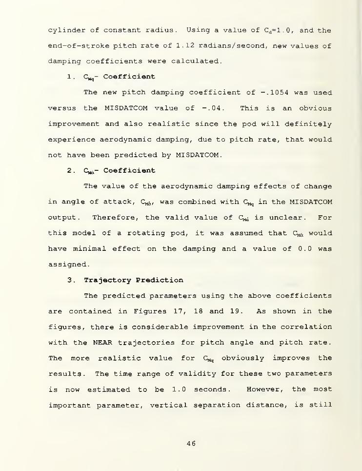
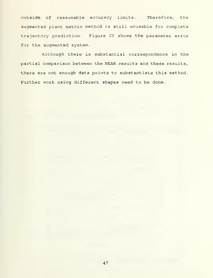
1. C„q- Coefficient 46

2. CMi~ Coefficient 46

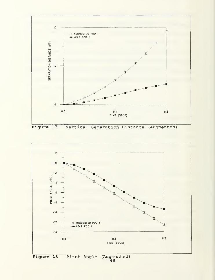
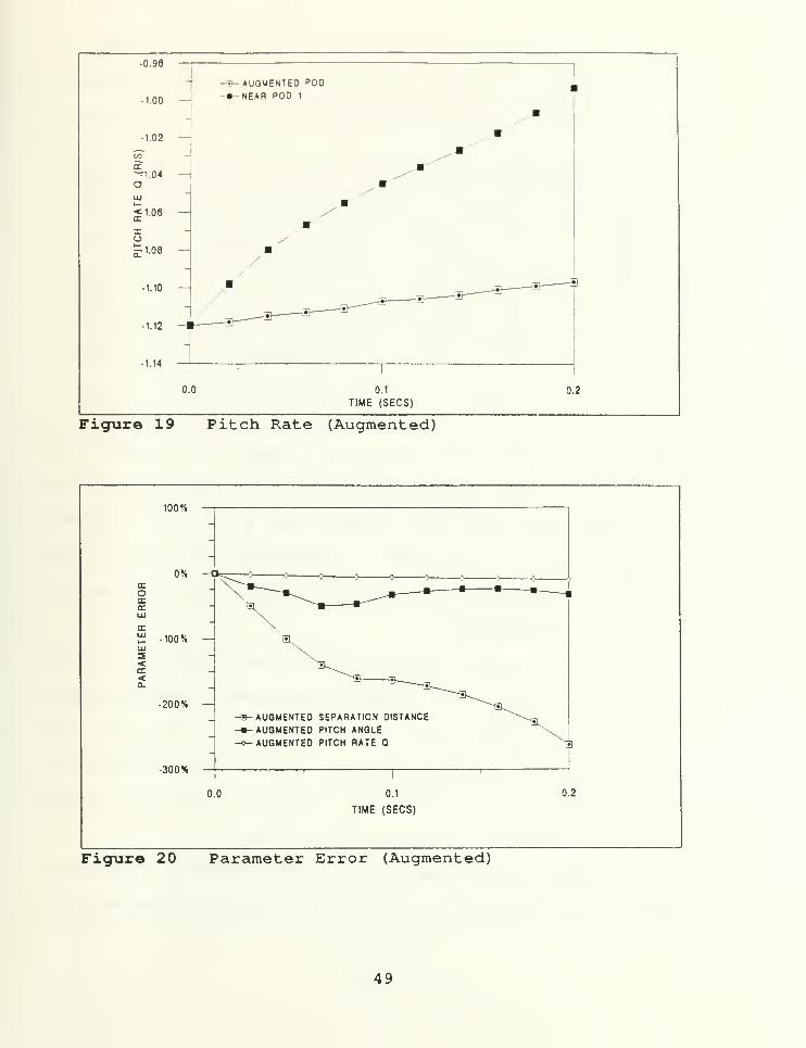
3. Trajectory Prediction 46

VI. CONCLUSIONS 50

APPENDIX A 52

APPENDIX B 53

APPENDIX C 55

APPENDIX D 60

APPENDIX E 61

LIST OF REFERENCES 66

INITIAL DISTRIBUTION LIST 68

VI

LIST OF FIGURES

Figure 1 Ejector Force 7

Figure 2 MISDATCOM Pod Shape 18

Figure 3 MISDATCOM Input 18

Figure 4 MISDATCOM Output 19

Figure 5 Pitch Angle Response 21

Figure 6 Pitch Rate Response 21

Figure 7 Vertical Separation Distance 22

Figure 8 Vertical Velocity 22

Figure 9 F/A18 NEAR Polynomials 2 9

Figure 10 Source Program Input 32

Figure 11 Source Program Output 34

Figure 12 Trajectory Program Partial Output 37

Figure 13 Trajectory Output (Cont) 38

Figure 14 Vertical Separation Distance 43

Figure 15 Pitch Angle 43

Figure 16 Parameter Error 44

Figure 17 Vertical Separation Distance (Augmented) . 48

Figure 18 Pitch Angle (Augmented) 4 8

Figure 19 Pitch Rate (Augmented) 4 9

Figure 20 Parameter Error (Augmented) 49

Figure 21 Store Reference Frame 55

Figure 22 Control-C Program For EOM Simulation ... 60

Figure 23 MISDATCOM INPUT/OUTPUT 61

VI i

Figure 24 MISDATCOM Input/Output (Cont) 62

Figure 25 MISDATCOM Input/Output (Cont) 63

Figure 26 MISDATCOM Input/Output (Cont) 64

Figure 27 MISDATCOM Input/Output (Cont) 65

Vlll

LIST OF ABBREVIATIONS AND ACRONYMS

axial force coefficient

drag coefficient

lift coefficient

yawing-moment coefficient

rolling-moment coefficient

normal-force derivative wrt to AOA

pitching-moment derivative wrt to AOA

side-force derivative wrt to beta

yawing-moment derivative wrt to beta

rolling-moment derivative wrt to beta

pitching-moment coefficient

pitching-moment derivative wrt to AOA rate

pitching-moment derivative wrt to pitch rate

yawing-moment coefficient

normal-force coefficient

normal-force derivative wrt to AOA rate

normal-force derivative wrt to pitch rate

side-force coefficient

maximum store diameter

g gravitational constant

I xx mass moment of inertia about the x-axis

I mass moment of inertia about the y-axis

I zz mass moment of inertia about the z-axis

IX

cA

c D

c L

^LN

ciL

^NA

c

C Y p

CinP

CilP

c m

c •

cmq

c n

c N

c .

^Nq

c Y

d

1 body (or store) length

1 R reference length

m body contour slope

M,„ free-stream Mach number

q.,, free-stream dynamic pressure

S local body cross-sectional area

S R reference area

t time (seconds)

VM free-stream velocity

x.r Y.r z « store coordinate system

xb> Ybf z b aircraft body coordinate system

a fuselage or store angle of attack

P fuselage or store sideslip angle

ACKNOWLEDGEMENT

I would like to thank the faculty of the Aeronautical and

Astronautical Department at the Naval Postgraduate School for

providing me with such professional insight into the field of

aeronautics. I especially want to thank my thesis advisors, Prof.

0. Biblarz and Prof. L. Schmidt, for continually providing guidance

and direction in my search for the elusive truth.

Rony Salama, a fellow student, was also instrumental in

validating my results by use of his practical knowledge in the

field of store separation.

In addition, my thesis work would have been impossible

without the able assistance of Tony Cricelli, who helped me

navigate the labyrinth of computer paths.

And most importantly, I want to thank my wife, Victoria, for

supporting her "ghost" husband for the duration of this thesis.

xi

I . STORE SEPARATION INTRODUCTION

A . BACKGROUND

The prediction of the trajectory of a store ejected from

an aircraft is of major concern to defense aviation. The

increasing requirement for aircraft to fulfill a multiple role

in the hostile environment demands that it also carry an ever-

increasing variety of stores. These stores range from

missiles and bombs stockpiled for many years to new,

aerodynamically complex stores with lifting bodies.

The aim of this work is to review current methods of

predicting store releases, compare results of two different

methods, and to present an easy-to-use methodology for

investigating the subsonic release of a unsophisticated store.

A non-axisymmetric pod ejected from the F/A-18 outboard

pylon is presented as an example. This store was chosen

because it is of practical value due to the extensive use of

these modified pods at the Pacific Missile Test Center, at

Point Mugu, California. Non-axisymmetrical stores are very

difficult to model and present a special problem in the store

separation field. This pod is, therefore, modeled as

axisymmetric and non-axisymmetric, and the results are

compared. In addition, the store lacks aerodynamic control

surfaces and is highly unstable. Application of the

methodology presented here should eventually provide the user

with accurate results for a minimal time and cost expenditure.

B. MATHEMATICAL MODELING

There are many ways to mathematically model store

separation. Economics and accuracy are always the main

considerations when exploring the codes and methods to be

used. For simple cases, intermediate approaches such as panel

methods and solutions of the Euler equations provide

sufficient accuracy. Calculations involving flow separation

and shock wave interference become too complex for

intermediate methods and acceptable results can only be

obtained using modern computational fluid dynamic (CFD)

techniques involving solutions of the Navier-Stokes equations

[Ref. l:p. 7-2]. For speeds below the subsonic Mach critical

speed, component buildup methods (empirical and semi-

empirical) , and panel methods provide the necessary accuracy

and are much easier to use. The codes chosen for this study

are explained in detail in their respective sections

.

The F/A-18 model was obtained from Mr. L. L. Gleason of

the Ordnance Systems Department, Naval Weapons Center, at

China Lake, California. The F/A-18 was chosen due to its wide

variety of store carriage and also because of its solid future

with Naval aviation.

The store model is based upon both the Missile Datcom

method [Ref 2] and also by the Nielson program [Ref 3] . These

will be discussed in Sections III and IV. Appendix A contains

the physical description of the pod and its inertial

characteristics

.

C . METHODOLOGY

The initial investigation (Section II) consisted of

looking at the ejector forces, combined with the store's

inertial characteristics, to give a sense of the magnitude of

initial velocities and moments. These forces and moments,

while easy to predict, were insufficient to provide real

evidence of a safe release or of a release problem. A large

pitch-down moment or a large vertical velocity may be off-set

by unforeseen aerodynamic forces . The velocities and moments

calculated will be used in Section III and compared with

results of Section IV for trajectory prediction.

Section III introduces a method of predicting the store's

longitudinal and lateral aerodynamic coefficients using a

missile code (Missile DATCOM) developed by McDonnell Douglas

Missile Systems Company for the Flight Dynamics Laboratory

(FDL) , Wright-Patterson Air Force Base (WFAFB) , Ohio [Ref . 2] .

These aerodynamic coefficients are then used in longitudinal

and lateral equations of motion to predict the free-stream

trajectory of the store. A brief explanation of the

derivation of these equations of motion is provided to the

reader. An accurate representation of the aerodynamic

characteristics is essential for the full prediction of the

shape's trajectory. Missile DATCOM is based on the body

buildup method and includes a number of prediction methods for

each component of the configuration. Other codes, such as

MISL3, are also available, each with its own relative

strengths

.

Section IV describes a computer prediction method

developed by Nielson Engineering and Research, Inc., (NEAR),

also under contract to the United States Air Force. This code

provides a six degree-of-freedom (6D0F) simulation which takes

into account the aircraft flowfield using vortex-lattice and

panel methods. The NEAR simulation provides a high fidelity

representation for the subsonic case, but also requires the

most effort and computer capability. An attempt has been made

to minimize the complexity of the input to the program. Once

a good data base has been developed the NEAR code should prove

easy to use. It has been used extensively throughout the

defense industry, and has undergone many modifications to

incorporate improvements and options.

Section V compares the trajectory results of the

linearized aerodynamic simulation method and the NEAR code.

A modification to the linear coefficients used in the linear

aerodynamic simulation is also discussed.

II. EJECTION FORCES AND MOMENTS

Although quite uncomplicated in nature, calculating the

ejection forces and moments provides the user with a feel for

the magnitude of the initial movement of the store. This

procedure should be done prior to using any other method as a

preliminary step in order to prepare for the simulation.

A. EJECTOR CHARACTERISTICS

The non-aerodynamic forces involved in the ejection of a

store depend upon the ejector cartridge, the ejector rack, the

weight of the store, and the rigidity of the wing. Each of

these parameters determine the resultant moments and forces

provided to the store. The store and the wing (or fuselage)

were considered as rigid, thus neglecting any aeroelastic or

structural bending effects. None of the methods discussed

here address aeroelastic bending due to the added complexity

of the problem.

The Douglas production BRU-32/A Bomb Ejector Rack combines

two sets of hooks, one set at 14-inch spacing and one set at

30-inch spacing, with an ejection system designed for carriage

of stores with suspension lugs per MIL-A-8591. Two

electrically initiated CCU-45B cartridges are used for store

release and ejection. The self-retracting ejector pistons,

spaced symmetrically 20 inches apart at each end of the rack,

have a piston stroke of six inches. These pistons are spring

loaded against the store during loading to prevent impact of

pistons during firing. The orifice sizes can be varied, by

replacement, to provide force and pitch control for store

separation. [Ref. 4]

The best source of ejector data is from the Aircraft

Ordnance Procedures (AOP) contained in the Aircraft Stores

Interface Manual, (Reference 4) . This manual contains a

complete description of the rack under consideration. Here,

the example separation uses two 14-inch spaced hooks and

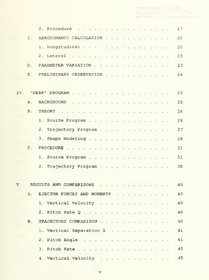
. 118-Diameter orifices. The force diagram corresponding to

this orifice, modeled from the AOP, is shown in Figure 1.

Sufficient data points were read from the AOP graph in order

to curve-fit the points using Computer Associates'

CricketGraph* software [Ref. 5]. This provided two things;

1 . ) integration of the polynomial equation gave the total

impulse value, and 2.) Nielson software in Section IV uses a

fifth-order polynomial for calculations. Note that the AOP

shows the total force provided by the ejector, while the NEAR

simulation requires a force-per-e jector-foot polynomial.

Given the shape of the force curve, a triangular

representation of the curve gave a value of 348 lb f-sec versus

the integrated value of 344.9 lb f-sec, which corresponds to an

error of only 1%. Therefore elementary estimates of the total

impulse are practical.

CO

UJOa:O

8000

7000

6000

5000

4000

3000

2000

1000

-j

0.000 0.010 0.020 0.030 0.040 0.050

TIME (SECS)

Figure 1 Ejector Force

B . FORCES

1

.

Theory

Using the conservation of linear momentum theory

presented in Appendix B, the pod was modeled as a simple beam.

The weight was concentrated at the center of gravity and the

resultant ejection forces were placed at the ejector feet

locations. The ejection force time histories are treated as

an equivalent force impulse which results in a change in

linear momentum as shown by the following equation:

JlF z dt = G2- G1

= (M*VS ) 2- (M*V.) J

The integral for representing the linear impulse is

based upon the fifth-order polynomial force time history shown

here

.

y= 280. 2-608022. 8x + 180688545 . 8x 2 - 10638451765 . 5x 3 +

234526098234. 3x 4 - 1783873760363 . 4x 5

2 . Example

For our example, the BRU-32A bomb rack used two CCU-

45B cartridge-activated devices (CADS) . The peak force was

14,500 lbf and the pulse duration was 50 msec. The total

linear impulse calculated was 345 lb f-sec . Using a weight of

371 pounds for the pod, the end-of-stroke velocity was 29.9

feet per sec (fps) . This value was used in Section III as the

initial velocity for the trajectory simulation.

The graphs contained in the AOP shows end-of-stroke

velocity for a 371 lb store to be approximately 24.5 fps

.

This graph is derived from empirical data and should provide

the most accurate representation of the actual release

velocity. The values of 24.5 and 29.9 fps are compared with

the end-of-stroke store velocity of 30.9 fps predicted from

the NEAR code in Section IV.

C . MOMENTS

1

.

Theory

The pod was modeled as a simple beam. The inert ial

characteristics of the store are listed in Appendix A. The

two ejector feet provide the beam with a moment. The

equations used are elementary, and with certain assumptions

the angular velocity can be calculated. The equations are

based on conservation of angular momentum. The equations and

assumptions are presented in Appendix B for completeness. The

resulting equation is shown here.

jlMy dt = iyy * (^

2 . Example

The center of gravity was offset aft of the center of

the ejector feet by 4.05 inches. The impulse thus provided

the pod with 1.12 radians per second (rps) or 64.1 deg/sec

initial angular velocity. The question now is, are these

reasonable values? At the end of 0.429 seconds, the shape

will be one body-length below the aircraft. At the same time,

the shape will have rotated 27.5 degrees nosedown. Therefore,

without considering the aerodynamics of the vehicle, the pod

seems to have cleared the wing. A good rule of thumb is 2-3

body lengths clearance, although exceptions do occur.

D. PRELIMINARY OBSERVATION

This initial calculation provides an approximate estimate

of the forces and moments involved. The values obtained are

of sufficient accuracy for calculations such as end-of-stroke

loading, etc. Excessively large separation velocities are

usually an indication of a miscalculation. Translational

velocities should range from 10-30 fps and pitching velocities

from 0-6 rps

.

10

III. AERODYNAMIC CALCULATION

A . THEORY

Many physical systems can be modeled by second-order

differential equations. The mathematical treatment of fixed-

wing flight vehicle motions was first developed by G.H. Bryan.

He laid the mathematical foundation for airplane dynamic

stability analysis, developed the concept of the aerodynamic

stability derivative, and recognized that the equations of

motion could be separated into a symmetric longitudinal motion

and an unsymmetric lateral motion. Experimental studies were

initiated by L. Bairstow and B.M. Jones of the National

Physical Laboratory in England, and by Jerome Hunsaker of the

Massachusetts Institute of Technology to determine estimates

of the aerodynamic stability derivatives in Bryan's theory.

In addition to determining stability derivatives from wind-

tunnel tests of scale models, Bairstow and Jones

nondimensionalized the equations of motion and showed that,

with certain assumptions, there were two independent

solutions, i.e., one longitudinal and one lateral. These two

solutions provide the free-stream trajectories we seek. [Ref

.

6:p. 113]

The dynamic stability characteristics of a pod can be

represented by six equations of motion, three for the forces

11

involved X, Y, and Z and three for the moments L, M and N.

The force equations relate the forces acting on the body to

the corresponding linear accelerations and the moment

equations relate the moments to the corresponding angular

accelerations. It is usually possible to consider the

longitudinal motions completely separately from the lateral-

directional motion, by neglecting the various coupling terms.

[Ref. 7:p. 14]

As a caveat to the use of this method, these equations are

the linearized version and are only valid up to approximately

10 degrees angle-of-attack . Treatment of the non-linear

aerodynamic coefficients, while not extremely difficult, does

require knowledge of the behavior of the coefficients. Since

the goal of this report is to predict the behavior of new

shape configurations, this knowledge is not presumed.

Therefore, the results obtained in this fashion are only valid

for estimating the motion in the first fractions of a second.

These results are compared with those obtained in the more

rigorous method of Section IV.

1 . Longitudinal Equations

The rigid-body, longitudinal equations of motion can

be developed from Newton's second law:

^Pitching moment3=2^^=1^*0

The assumption that body motion consists of small deviations

from its equilibrium flight condition allows us to use

12

perturbation theory to examine the aerodynamic force

derivatives in terms of angle-of-attack (AOA) , vertical

velocity, pitch angle, and pitch rate, by means of a Taylor

series expansion. The X-force, Z-force, and pitching moment

equations comprise the longitudinal equations . To separate

these equations from the lateral equations, they must not be

coupled. This is a reasonable assumption given the nominal

geometric shape of missiles or pods [Ref . 6] . The body is

constrained to move in a vertical plane and is free to pitch

about its center of gravity. For a comprehensive derivation

of the equations of motion, see Reference 6. The resulting

equations of motion are shown in Appendix C.

2 . Lateral Equations

The Y-force, rolling, and yawing moment equations

comprise the lateral equations of motion. Once again, these

equations are uncoupled from the longitudinal equations by the

assumption of small cross-component moments of inertia. That

is, I xy , I xz , I yx are small in comparison to the principal axis

moments. These equations are also valid assuming only small

variations in displacement and velocity. The lateral

equations are derived from the following Newton's laws:

ZRolling moment s=1^*0

ZYawing moment s= I „*\|/

The third equation is derived from the Taylor series expansion

of the side force derivative. The lateral motion of the pod

13

disturbed from its equilibrium state is a complicated

combination of rolling, yawing, and sideslipping motions.

Assuming the cross products of inertia are ignored, some of

the coupling terms can be simplified.

3 . State Variable Representation

The linearized longitudinal and lateral equations

developed above are simple, ordinary linear differential

equations with constant coefficients. The coefficients in the

differential equations are made up of the aerodynamic

stability derivatives, mass, and inertia characteristics of

the pod. These equations can be written as a set of first-

order differential equations in the state-space (state

variable) form:

{x} = [A]*{x} + [B]*{T1}

where {x} is the state vector, {T|} is the control vector and

the matrices [A] and [B] contain the pod's dimensional

stability derivatives. In our case the pod does not have any

active control surfaces. For missile launches, however, the

control vector and the B-matrix would be used to represent the

control surfaces and control input. The simplified state-

space representations of the longitudinal and lateral

equations of motion are shown in Appendix C. The required

14

coefficients listed in Appendix C are derived using the

procedures in Section III.B.

The state-space representation of the equations of

motion can be solved simultaneously using matrix software such

as MATLAB* [Ref . 8] or Control-C* [Ref . 9] . Given the

conditions of the ejection, namely, initial translational

velocities, initial angular velocities, and attitude angles,

solutions of the state-space equations can be used to predict

the trajectory of the pod. The initial angles and velocities

are the initial conditions imposed upon the state-space

equations. The Control-C* commands for this procedure are

contained in Appendix D

.

B. MISDATCOM

MISDATCOM was developed by McDonnell Douglas Astronautics

Company, St Louis, Missouri, for the Flight Dynamics

Laboratory of the Air Force Wright Aeronautical Laboratories,

Wright-Patterson AFB . The program was completed in December

1985. The Missile Datcom was created to provide an

aerodynamic design tool which has the predictive accuracy

suitable for preliminary design, and the capability for the

user to easily substitute methods to fit specific

applications. [Ref. 2:p. 1]

1 . Theory

There are many different methods to predict the

aerodynamic static, dynamic, and control characteristics of

15

missiles. Component build-up was chosen as the most suitable

for this program. Although panel methods are better suited

for arbitrary configurations, component build-up was chosen

due to the accuracy provided for conventional configurations

and for the ability to do parametric studies easier.

Basically, component build-up consists of using

various methods to compute the characteristics (skin friction,

force and moment coefficients, panel loading, . . .) of the

individual configuration components. The various methods are

chosen for their applicability to the configuration or flight

condition. Then the components are combined. Previous

methods of combining the components (fins, body, engine inlet)

consisted of adding the individual coefficients and then

multiplying the sum by some interference factor obtained using

slender body theory. The approach t~ken with MISDATCOM was to

use the "equivalent angle of attack method" developed by

Nielson Engineering and Research, Inc. (NEAR) . This method

assumes that the panel loading for a given panel angle-of-

attack is unique. With this method the panel angle of attack

is computed including the effect of panel roll orientation

with respect to the free stream velocity vector, panel

proximity to the fuselage or to other panels, and external

vortex flow field effects. Then the isolated panel

characteristics are interpolated at the panel equivalent angle

of attack to yield the panel load when mounted on a body in

combination with other surfaces. [Ref. 2]

16

2 . Procedure

The procedure for using MISDATCOM is straightforward.

The pod shape is modeled using simple geometric shapes. The

previous release of MISDATCOM software could only handle

axisymmetric shapes or forms with a vertical plane of

symmetry. Unfortunately, the pod under consideration is non-

axisymmetric and therefore the results are not entirely valid.

The latest version, however, can model some non-axisymmetry

through the use of a "protuberance" option. This is the April

1991 release and is now available.

For this investigation, a simulation run was made

using both versions and a comparison of the aerodynamic

coefficients was made. The pod radius was also varied from

the minimum pod to the maximum, and the resulting coefficients

compared. The MISDATCOM code coefficients were somewhat

insensitive to radius changes of this magnitude, therefore,

the minimum-radius, axisymmetric case was retained for

comparison with the minimum-radius non-axisymmetric case.

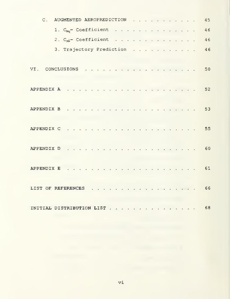
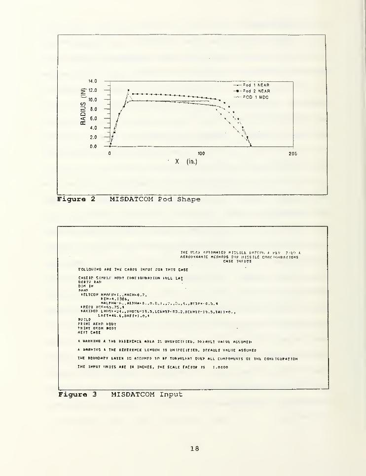
Figure 2 shows the pod semi-profile of the MISDATCOM procedure

alongside the pod semi-profile of the NEAR simulation. Figure

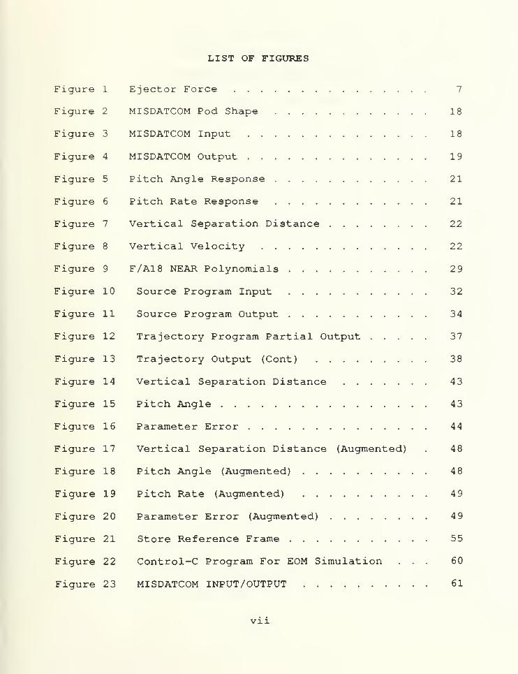
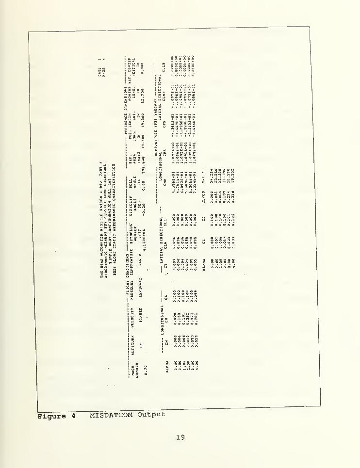
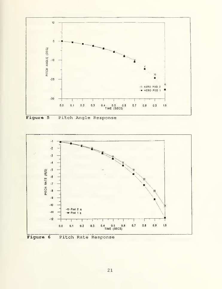
3 contains a sample input to the program and Figure 4 lists a

partial sample output. The actual input and output of the

program are contained in Appendix E. These aerodynamic

coefficients are next used in the longitudinal and lateral

state-space equations of motion to predict the store

trajectory

.

17

14.0

£-12.0

""10.0CO

3 8.0

Q< 6.0tr

4.0

2.0

0.0

— Pod 1 NEAR

-•-Pod 2 NEAP,

---POD 1 MDC

100 200

(in.)

Figure 2 MISDATCOM Pod Shape

THE U'.r.fc MIIONMEli MCLILL DAT/COfi * KtU 7/f'J *

AERUHYNAMIC MCIHOI'S F'tP MISSILE COHf WIRAT IOMScase mruis

FOLLOUING ARE THE CARDS INTUT fOR THIS CASE

caseit sinrt.i: mody cmhi igmraj ion hill lajDERIV RADDIM IN

DAMP•ELTCOH NMOf |t*l . ,HACH*0.7,

REN-.*. 13E&,N ALPHA- f..

, ALPHA* 0. ,0.8, J . ,H. , S. , 1. ,tl:tft»- O.b, •• RETO XCr, = »ib.75,«» AX I POD LNaSM'J4.,UM0rtM9.3,lCKNTr*n3.3,tlCFNlR>-|9.S,TAtl«0.

,

LAET>46.6,DArt*I.0,tIUILDHINT AEPO HOUYPRINT GFOM *OPYNEXT CASE

* WARNING A THE PIEEPENCE APfc.fi It UNSPEC IP 1EU. DUAULT vol ut A'J'.UHEI'

A UARNIMG A THE DEFERENCE LENGTH IS UNSPECIFIED, PTFAULT VALUE ASSUMED

ihe ioutmArr layer ic ArruMFi' to »f turhiilpnt over all components of the coni igupatioh

THE INPUT UNITS ape IN INCHES, IHE SCALE FACTOR IS 1.0000

Figure 3 MISDATCOM Input

18

I...I ui 4t M (J X OI x - - oI ui •-• o I :J

o o o o o oooooooooooooo o o o o o

a I Uto o -•

« —Jl M at

> 3 « Mu .J i I-

1 - u

w * »« e © o o o oX X 13 r o I t J

O UJ z VI 1 UJ X. UJ Uj** x C3 fv X •N JJ Jl * r« J)

VI o ~l -• ff- T- <T <r <r cdX c Wl n 1

1

O o O a o oMM -a Xc «

•I t i

a,

a<

--

Ulw z »-* X © v*

U H «t o < o O O o O ©x o «1 m -J 1 1

ut X UJ a jj UJ UJ MH Ul <r *- >- -o <r n cd OUJ -I 1

1

J3 ^ n J> -*It* Ml J) IN. «f n *

M W OHI SOI -J -1

I < «1 1U Ul « C9I Jl* I *I

a- «T -• O

5 I I I I I I

« — -4 -. M -. -.

D> © © © o © o- *M <1 w iiu jiui ji

j) j C r j; <n — n src<u (T o- <r tr x r-

X o o o o o o

© © o o © cI I I I I I

Ul -jJ Ul JJ U JJj-fir a*r« s cr o o rt

n tN o j> n o«* <r vi ^i «j) is

«r <jb <j) o onn J o * r o

O H /l T «r »o nj n n^© o o - ri no o o © o o

a t/> h *tn « <

ui -» X-i r 3 v-

m o an * - oHOhiN-j. i ji

c O «t

(A t JOS (JW O >• HH X a Hc *-• o «Cw*hOff tl

H ui

r u -i ui

< — •• xX K O

u. C - -I

3 a »-

o aUl M O

- w *- JJ

C • M ©I X ^>- 3 -* ui

< -IX -Io ->

o o o o © o© o o o o o© o © o o oo © © © o ©

« aj J> JJ aj m O—

-

(f» gl J* gft (fi |wj

©X oooooo•J

-JCJ oooooo

« V * r> tti

o © © © o O© © © o o oO 9 O © O ©

o o © o - «oooooooooooo

O o o -• ;i noooooooooooo

O o -+ f • n *

t uI a

I x uI uI « cI r 3

o o o o o <rO O O O O ff»-.-.-.-.-. ooooooo

-• © r» *- r • r« --•

O Oil (MDh Jl3K onnniiho o O O © ©

O Jl D f. n IT

oooooooooooo

ooHfin*

Figure 4 MISDATCOM Output

19

C. AERODYNAMIC CALCULATION

1 . Longitudinal

The aerodynamic coefficients derived from the

MISDATCOM were entered into the plant matrix [A] of the

longitudinal equations of motion. The initial conditions were

applied and time history of the pitch angle, pitch angular

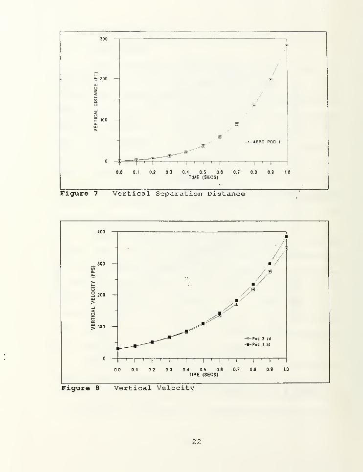
velocity, and vertical velocity was found. Figures 5-8 show

that the pod assumes a large nose-down, highly divergent

pitching motion. This is understandable since there are no

control surfaces to make the pod stable. Examination of the

roots of the plant matrix [A] indicates an unstable flight

vehicle. The pitch angle and pitch rate shown are in the

store body coordinate frame.

These results are valid only for the range of linear

values of the aerodynamic coefficients. This is approximately

up to 10-12 degrees angle-of-attack. Therefore, an estimate

of the non-linear behavior of the pod after an AOA of 10

degrees is reached is necessary. Due to the large pitch

angular velocity, it is obvious that this limit is reached

after only 0.2 seconds. Section V discusses the acceptable

time range where these results are valid.

To estimate the non-linear behavior, the dominating

terms in the [A] -matrix must be determined. This provides an

insight into the possible range of values to substitute into

the [A] -matrix. A discussion of a possible approach to this

20

C3LUQ

10 —

•20 —

•30

\

-- AERO POO 2

-•-AERO POD 1

1 r "ii

r"i——

r

0.0 0.1 0.2 0.3 0.4 0.5 0.6 0.7 0.8 0.9 1.0

TIME (SECS)

Figure 5 Pitch Angle Response

-i

•2 —

•3

•4

z •t—

2 -7

xg -8

Q.

-9

-10 —

-11 —

-12 —

a

-a?- Pod 2 q

-m-Poi 1 q

0.1 0.2 0.3 0.4 0.5 0.8

TIME (SECS)0.7 0.8 0.9

I

1.0

Figure 6 Pitch Rate Response

21

JUU

1?

/

i.200

/

/15

ill

oz<GO

a

//

/rsi

_i<K 100DC

—IE

>

_„^—(•/

S*Y

^®-J- AERO POO 1

__—T)—

~

—-—(•J'""'"'""

- T 1 1 1i

1

i i

'

I' I ' i

0.0 0.1 0.2 0.3 0.4 0.5 0.6 0.7 0.8 0.9 1.0

TIME (SECS)

Figure 7 Vertical Separation Distance

400

300 —

200 —

<

100 —

-™>-Pod 2 id

--Pod 1 zd

i 1 1 1 1 1 r -i—i—

r

0.0 0.1 0.2 0.3 0.4 0.5 0.6 0.7 0.8 0.9 1.0

TIME (SECS)

Figure 8 Vertical Velocity

22

problem is presented in Section V. To completely investigate

this area is beyond the scope of the method outlined here.

Comparison of the "linear" trajectory obtained here will be

made with the trajectory obtained in Section IV, which does

take into account the non-linearity of the coefficients.

2 . Lateral

Due to the nearly vertical forces and moments provided

by the ejection rack during straight and level flight, the

free-stream lateral equations of motion will not provide us

with any insight into the safe jettison of the shape.

However, if the pod were experiencing sideslip, then the

sideslip could be entered into the state-space equations as an

initial condition. For this pod a sideslip of -0.5 degrees

was assumed. The resulting lateral motion is not shown

because the main emphasis is on the longitudinal motion. The

pod is unstable laterally, also, but the initial movement is

small due to the relatively small initial conditions. In

addition to the yaw angle and rate, if the ejection rack

provided an initial roll rate, such as when the pod is loaded

off-center of the bomb rack, then that influence could also be

included.

D. PARAMETER VARIATION

The parameter variation due to non-axisymmetry is

difficult to handle. Comparison with shapes with known

23

(experimentally obtained) coefficients might provide some

degree of accuracy in predicting more accurate results

.

E. PRELIMINARY OBSERVATION

The results of the method in Section II were a vertical

velocity of 29.9 feet/sec and an angular velocity of 64.1

deg/sec. The aerodynamic method of Section III begins with a

vertical velocity of 29.9 fps, quickly diverging to an

extreme value. The pitch rate, q, also diverges quickly.

Because the pod is very unstable any linear approximation of

its behavior will have strict limits . The coefficients used

in this calculation, from the MISDATCOM code, are not valid

beyond a fraction of the trajectory. The valid time range of

prediction is presented in Section V.

24

IV. "NEAR" PROGRAM

A . BACKGROUND

A computer prediction method was developed by Nielsen

Engineering and Research, Inc., (NEAR) under contract to the

United States Air Force. The work was performed during the

period 1968 to 1972. The final result is a method for

predicting the six degree-of-freedom store separation

trajectory at speeds up to the subsonic critical Mach number.

After delivery of the program to the Government, many new

capabilities were added. The code used for this paper was

obtained from the Naval Weapons Center, China Lake, Ca. The

program has been widely accepted by industry and government.

The code encompasses 9, 900 lines of code and thus requires a

device with sufficient computer memory for operation. (This

also depends upon the program application.)

The aircraft fuselage, separated store body, and adjacent

stores are modeled using point sources and sinks. Angle of

attack effects are included using a cross-flow model . The

aircraft wing and wing pylons are modeled using planar vortex

lattice models which include dihedral, camber, and twist of

the aircraft wing. Thickness strips are used to model the

thickness of the aircraft wing and pylons. [Ref. 10 :p. 807]

25

The capability exists to install multiple sets of wings,

fins, or canards, and to use active control surfaces on the

store by inputting the control laws into the program. Powered

separations may be simulated by inputting the store thrust

characteristics

.

The NEAR program actually consists of two separate

programs: the source program and the trajectory program. Both

are described in Section IV. B below.

Alternate separation programs include USTORE and USSAERO

codes. USSAERO was developed by F . A. Woodward, of NASA, as

a lower-order panel method. USTORE was developed from USSAERO

by G. J. van den Broek, of the National Institute for

Aeronautics and Systems Technology, Pretoria, South Africa.

[Ref. ll:p. 309]

B . THEORY

The three principal tasks in the prediction of a store

trajectory are: first, the determination of the nonuniform

flow field in the neighborhood of the ejected store; second,

the determination of the forces and moments on the store in

this flow field; and third, the integration of the equations

of motion to determine the store trajectory [Ref. 3].

1 . Source Program

The source program is used to represent an

axisymmetric body as a distribution of sources along the axis

of the body. It provides point source-sink distributions to

26

represent the fuselage, rack, and store volumes. The program

calculates and prints the source strengths and locations.

These quantities are then used as input data to the trajectory

program.

The source program is used for the generation of an

aircraft or pylon model which is then used for the trajectory

program. These models are Mach number dependent and thus need

to be generated for each test case with different Mach number.

For ongoing store separation studies, a good database of

aircraft models is required and should be available from

appropriate Government facilities. The F/A-18 model was

obtained from China Lake along with the program code. This

model included pylon stations.

2. Trajectory Program

The trajectory program uses the source-sink

distributions from the source program, and additional

information to first determine the vorticity distribution

which represents the wing-pylon loading including interference

of the fuselage, rack, and stores, and then to calculate the

store trajectory. See Sections IV.C.3.d.(l) and (2) for

descriptions of the vortex lattice method and the panel

method.

Once the trajectory program input has been generated

for a single flight condition, it is relatively easy for the

user to input different stores. The major effort is to obtain

27

the initial aircraft fuselage, wing, and pylon models for this

input

.

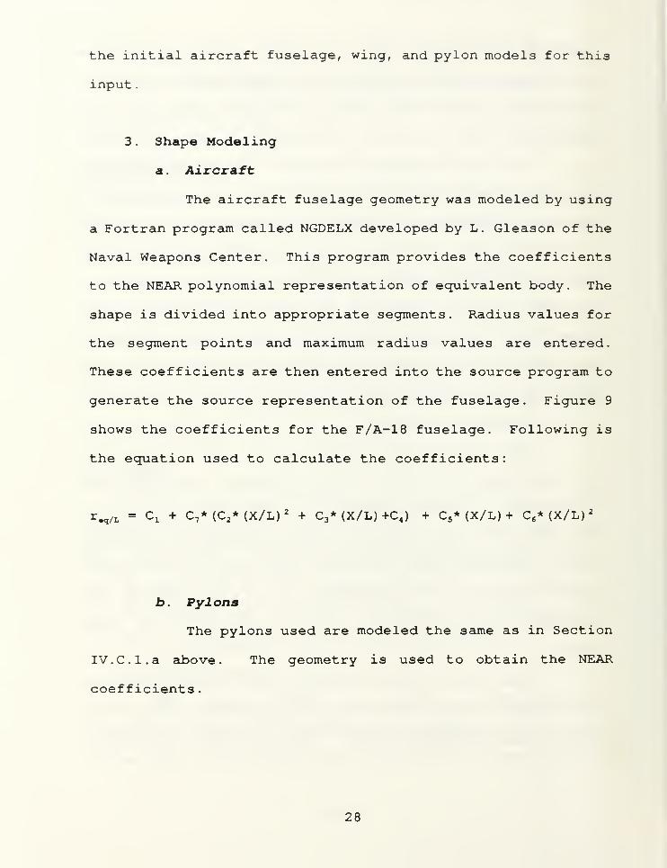
3 . Shape Modeling

a . Aircraft

The aircraft fuselage geometry was modeled by using

a Fortran program called NGDELX developed by L. Gleason of the

Naval Weapons Center. This program provides the coefficients

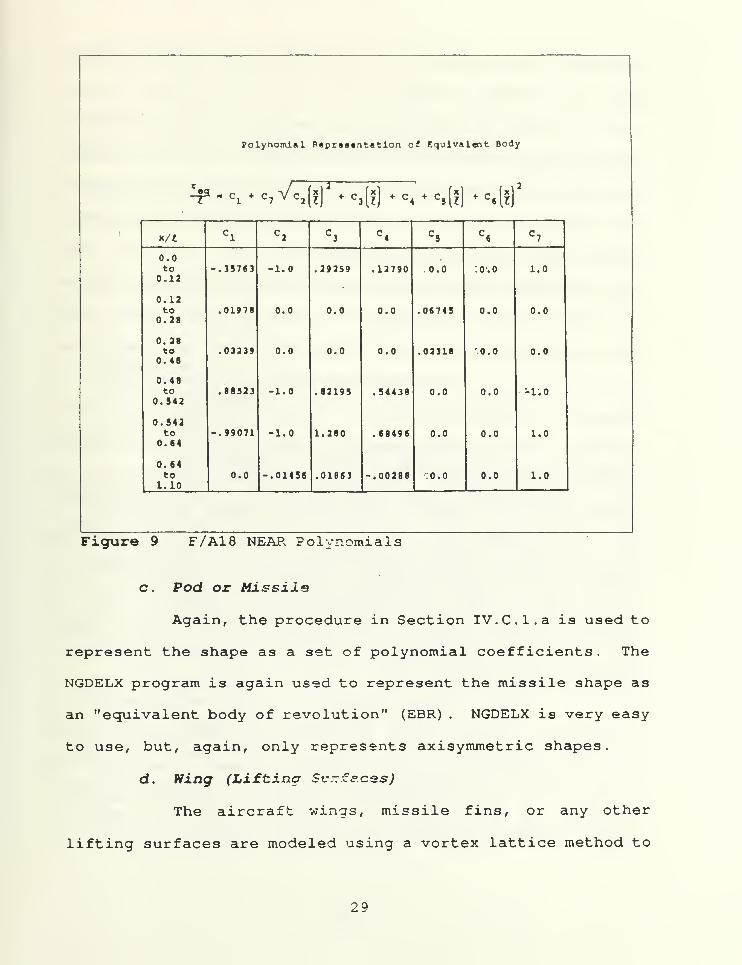
to the NEAR polynomial representation of equivalent body. The

shape is divided into appropriate segments. Radius values for

the segment points and maximum radius values are entered.

These coefficients are then entered into the source program to

generate the source representation of the fuselage. Figure 9

shows the coefficients for the F/A-18 fuselage. Following is

the equation used to calculate the coefficients:

r.q/L = Cj + C7 *(C 2 *(X/L)2 + C 3*(X/L)+C 4 ) + C 5

* (X/L) + C 6* (X/L) 2

Jb. Pylons

The pylons used are modeled the same as in Section

IV.C.l.a above. The geometry is used to obtain the NEAR

coefficients

.

28

Polynomial Rapraatntatlon of Equivalent Body

!p.c1+ c

7Vc

a (f)

a+ c

3 (|)+ c

4+ c

5 (|] >c<[i)

*/LCl

C2

C3

C4

C3

C6

C7

0.0to

0.12-.35763 -1.0 .29259 .12790 . 0.0 :o.o 1.0

0.12to

0.28.01978 0.0 0.0 0.0 .06745 0.0 0.0

0.28to

0. 4B.03239 0.0 0.0 0.0 .02318 0.0 0.0

0.48to

0.542.88323 -1.0 .82193 .54438 0.0 0.0 -1.0

0.542to

0.64-.99071 -1.0 1.260 .68496 0.0 0.0 1.0

0.64to

1.100.0 -.01436 .01863 -.00288 :0.0 0.0 1.0

Figure 9 F/A18 NEAR Polynomials

c. Pod or Missile

Again, the procedure in Section IV.C.l.a is used to

represent the shape as a set of polynomial coefficients. The

NGDELX program is again used to represent the missile shape as

an "equivalent body of revolution" (EBR) . NGDELX is very easy

to use, but, again, only represents axisymmetric shapes.

d. Wing (Lifting Sv~£e.ces)

The aircraft wings, missile fins, or any other

lifting surfaces are modeled using a vortex lattice method to

29

represent the loaded wing. The thickness is also modeled

using the lattice method.

(1) Vortex Lattice Methods. There are several

variations of the vortex lattice method that are presently

available and have proven to be very practical and versatile

theoretical tools for the aerodynamic analysis and design of

planar and non-planar configurations. [Ref. 12 p. 27] The

vortex lattice method represents the wing as a planar surface

on which a grid of horseshoe vortices is superimposed. The

velocities induced by each horseshoe vortex at a specified

control point are calculated using the law of Biot-Savart . A

summation is performed for all control points on the wing to

produce a set of linear algebraic equations for the horseshoe

vortex strengths that satisfy the boundary condition of no

flow through the wing. The vortex strengths are related to

the circulation and the pressure differential between the

upper and lower wing surfaces. The pressure differentials are

integrated to yield the total forces and moments. [Ref. 13

p. 261] For a rigorous introduction to the vortex lattice

method, see Reference 13.

(2) Panel Methods. The configuration is

modeled by a large number of elementary quadrilateral panels

lying either on the actual aircraft surface, or on some mean

surface, or on a combination thereof. To each elementary

panel, there is attached one or more types of singularity

30

distributions, such as sources , vortices, and doublets.

These singularities are determined by specifying some

functional variation across the panel (e.g., constant, linear,

quadratic, etc.), whose actual value is set by corresponding

strength parameters . These strength parameters are determined

by solving the appropriate boundary condition equations. Once

the singularity strengths have been determined, the velocity

field and the pressure field can be computed. [Ref . 13.*p. 258-

259]

C . PROCEDURE

1 . Source Program

a . Input

The program input consists of the polynomial

representation of the equivalent body of revolution (EBR)

values obtained in Section IV.B.3.a. The surface of the EBR

is approximated by these polynomials, which represent the EBR

x,r distribution. The source program is then run with a user-

specified finite distribution. The surface obtained from this

source distribution can then be compared with the polynomial

surface. Additional runs may be required to closely match the

surfaces. The aircraft fuselage, pylon (s), and the adjacent

store EBR values are input along with two variables, NRAT and

PERCR. NRAT is the number of segments which the body will be

divided for the specification of the source distribution.

31

PERCR is the source spacing for each NRAT segment and is input

as a fraction of the local body radius of the segment

.

Adjacent stores are included in the aircraft source

input. In this way it becomes part of the aircraft

configuration. The separated store is not input to the source

program since the trajectory program calls the source program

during its execution to model the store. this is due to the

fact the store changes position during the program run and the

sources/sinks will change values. Figure 10 lists a sample

format for the source program input

.

FILE: 2-F18S0U T Al

lf-18 AIRCRAFT

1

1

F-18 AIRCRAFT

« 0.70

0.12 0.28 0.68 0.542 0.64 1 .0

-.35763 -1.0 0.29259 0.12790 0.0 0.0 1 .0

0.01978 0.0 0.0 0.0 0.06745 0.0 0.0

0.03239 0.0 0.0 0.0 0.02318 0.0 0.0

0.88525 -1.0 0.82195 0. S4438 0.0 0.0 -1.0

-.99071 -1.0 1.28 0.68496 0.0 0.0 1.0

0.0 -0.01456 0.01863 -.00288 0.0 0.0 1.0

0.001 1.1 0.4400 0. 1. 0.02 0.0555

«

0.1004* 0.15525 0.28311 0.37443 0.97717 1.0

O.C 0.8 1.0 1.2 .8 .8

Figure 10 Source Program Input

32

b. Output

The source program output is used as input to the

trajectory program. However, it is not directly read into the

trajectory input and must be entered via keyboard. The form

of the output is shown as a partial output in Figure 11.

Source locations and strengths are listed.

33

F-H »l«c»wi

X/L OF IMO POINT OF EACH SECTION OF »00Y

SECTION

x/l'

1114• . 12000 0.20000 O.<0000 0. 54200

COEFFICIENT* OF POLYNOMIAL OESCRKIMO EACH SECTION

ION CI

0.1*711

t.tn r%

(.01277

0.10*21

0.»»0M0.00000

C2

-1.00000

•00000

0.00000

-1.00000

-I .00000

-•.014*4

CI

(.1*231

0.00000

0.00000

0211*

I .20000

0.01141

C4

». 12779

0.00000

0.00000

I.14411

0. IKM-0.00200

*

.44000

C*

0.00000

I OIH!

0. 02) 10

0.00000

0.00000

0.00000

c<

0.00000

0.00000

0.00000

0.00000

o.ooooo

0.00000'

C7

I .00000

•00000

0.00000

-I .00000

I .00000

I .00000

FIRST JOURCE AT X/L" 0.00100

LAST SOURCE AT K/L • 1.10000

FROM 00100 TO loo<4 SOURCE SPACINO IS 40000PROM 10044 TO 10*1* •OURCt •PACIHO IS 00000FROM 1**2* TO 20)11 SOURCE SPACIHO IS 1 00000FROM 2(111 TO 17441 SOURCE SFACIHO IS 1 20000PROM 17441 TO 77717 SOURCE SFACIHO IS • 0000FROM 11111 TO 1 00000 SOURCE SPACIHO IS • 0000

TIMES LOCAL RADIUS

TtHCl LOCAL RAOIUSTIHES LOCAL RADIUS

TIMES LOCAL RADIUS

TIME* LOCAL RADIUS

TIHES LOCAL RAOIUS

FOR THIS CASe THERE ARE 74 SOURCES

SOURCE LOCATIONS AND (OOY RADIUS AMD SURFACE SLOFE AT THESE LOCATIONS

X/L O.OOIIt (.0011* (.00112 •.00170 (.00224 (.00241R/L «.000«» (.000*4 0.00047 •.00077 •00071 •.00104DR/OX (.40524 (.404*7 (.40777 (.402(7 •.401(0 •.400*4

K/L (.00141 (.00424 (.00477 • . 004(2 •00777R/L (.•0144 0.00171 (.00177 0.00272 •00717DR/DK •.17714 0.11*17 0. 11210 0. )070* 0. !0)J«

K/L (.01072 (.0127* (.•KM •.02017 •.02142R/L 00110 (.00414* •.00*77 •.•0740 g. 00171DR/DH (.17404 (.74(10 •.74147 •.14*74 •.71*49

K/L (.•7142 0.0)42* •.04172 •0*474 •.0427*R/L •.01127 (.01277 •.•147* •.01774 0.011*4DR/DK (.111*7 (.27707 •.21112 •.24*70 •.222*7

K/L 0.07107 00171 10021 •.12477 •.14112R/L •.•2101 «.«244« •.02401 020)4 0.02147DR/OX •.174*7 (.14(0* •.1200* •.•4743 •.•4743

K/L O.IOI74 •. 20444 0. 22(42 •2(012 10700R/L •.01204 «.OI7*t «.«l*2« 01O00 •••71*7OR/OK 0.04747 (.0474* •••743 I.MIII 02)10

K/L 174)0 (.17777 (.427*7 (.47214 41110R/L (.04111 (.04144 •.04221 (.04177 •.(4*01DR/DK .021 10) (.027K *.022l( 0.02)10 •.10227

K/L 7*7011 (.37771 0.110)2 (47147 (.70*11

R/L (.0*141 (.0*174 0.«*30« (.0**14 •.0*447

DR/DK (.0(424 (.037(2 (.(2(l( -(.000*7 -0.00007 -(.01772

X/L 1.71447 (.74747 (.77774 (.(2771 (.(5413 00440 (.71144

Figure 11 Source Program Output

34

2 . Trajectory Program

The trajectory program uses the output of the source

program, and the input of the wing configuration and pylons,

along with store information to calculate the trajectory of

the separated store. It is not the intent of this report to

fully explain the aircraft modeling details of the program.

The assumption is made that the appropriate aircraft model is

available for the correct flight condition and configuration.

The applicable store inputs to the program are discussed and

the resulting trajectory examined. Nielson contains a

thorough description of the theory and input of the aircraft

model in Reference 3

.

a . Input

The example input to the trajectory program was

1064 lines in size. The store data entry begins at

approximately 980 lines, depending upon aircraft input. The

store input will vary according to the physical configuration

of the store. For the example separation, Input Items 35-43

and 48-51 were used to input store physical data. The ejector

information was input in Items 44A-47. This is where the

fifth-order polynomial representation of the ejector force was

used. Data concerning initial and final times, and

integration step sizes were entered in Input Item 72 . The

correct input form of the above data is contained in the NEAR

code users manual [Ref. 14] and is not presented here.

35

b . Output

The output of the trajectory program is dependent

upon the input conditions, i.e., the number of stores, number

of store segments, and number of integration steps, etc. The

example case output is 4,524 lines. The first 1,840 lines of

output are aircraft-specific output, such as the source and

vorticity information.

The last 2,650 lines of code contain the trajectory

data. The ejector force data is repeated as is the store

shape data, reference dimensions and inertial characteristics.

Proceeding the ejector data, a data block is

presented for each time integration step. This data block

contains the parameters which describe the store displacement,

velocity, and acceleration during the separation. A partial

sample output of this section of the output file is included

in Figure 12. Plotting routines can be developed to

facilitate data analysis of the simulation but have not been

developed for this study. The following are short

descriptions of some of these parameters . A comparison with

the results of the method of Section III follows in Section

IV. D.

The force and moment coefficients are listed by

their individual contributions. The effects of buoyancy,

slender body theory, crossflow, and empennage are totaled to

give an effective CN , CY , C^, and C ln .

36

OOOO JjfciOH B«l»

trool .^r„,, M net 1

1

IHttACIII ,....,,I I -I. »«ll t «« ... »n-.

iri>'BII.II l»»"Bll.tl TftHSII.fl lt|IIB||.4| IM"OII.1l•. ••••«-• •.•••••• I.IUIt'N •••(.• • 1...1 .!

TIMl It THt IHOtftUOtMr tJtCIOH VMIAM.I

IFOOT Mtrolvilt "in liflMlll lnrwflllt I •»«• I |t HI III!

tftlfjll.ll lftHOII.II lff"OI|.|> tffHOII.41 lffHOII.il"HI H I.IHICII l.lilll'll ».gooofg| Liiio-gi

MH1 It IHJ. IMOfftMOtHI tJlCTOH v»«l»nf

eotrfieiemt of iih ecsott pn.mgniH>i

reef I el et ci ci ci c«

I I t.ittifti -• iii»' h i.iiiii'ii -i.iiiii'ii i.iiiii'it -t.irtttMl

CI ei

t. unfit -t.iaiifii

i. iigil-gi -•••it'llt t I l»9?f«l -• nigf-fli i.iigii'gi -•••it'll l.iHU'lt -•IIKfll110*1 ««!« | It IK li«i f ;fc'fO

AOOITIOHM. IMTUI ton TMI1 110ft

llOflt MMt • II mo H.U0I

MOHtmj «im ftooucn of ihiiiu. ji_uo - to nIKX • t.it

lr» • It.tl

lit • If. ll

IT • • no

1*1 • titIKY • t.tt

trout MOHtMt ctMitt it -t.411 fttr rf'inio wonttOUt HtfCMHCI »»f» it t.tt! 1l.fl.

tlOMf MffMMCt ItMOTH It I. til fl.

• TOtlt CtNItt Of OUAVIIY OTfJtl ftOM HOMfMI CtNltt. fttf

fl»t • t.iooot

vt«t • l.lllll

j»a» • t.totot

tOLYiio»i|»it trtcirviiia eOHr»titin.e tiont JHArt

HA. Of IHO Of fACH ttCTIOH

ttCIION I/I irff fit It • MO. 1 • tOLYI

1 1. 11*11 •

t I iiiii i

1 I.MIIt i

4 l.lllll t

1 I.II4II •

t l.ntai t

etjtffieifHit Of tOI.YMOm»l.1 Dt1C*ll|M<l lACtt ItCIION

•Ml ION CI Cf ci e« CI c< cr

1 •.•»••• • .••••• • •••it •••«•• •••••1 • ttttl •.•ooot

1 l.lltlf -i .»•«»• • 1 1004 -•••III ••0001 • • •••• 1 . •••»•

1 -i.iurt -i .«•••• • MHI ••.••lit !.••••• • ••••• 1 "«'M

4 I.II44I -i .••••• • mil -I.III4I •.••••• • •«••• l.tttll

Figure 12 Trajectory Program Fartial Output

37

PILt 11X11

ii'f • imi iihcp • i oooo (iihi • i.otoi

IIH1 • •.lllll ICCC4IDI

Pone* amo H-fini coerptciiHtl iaip. amca • on pi«-i — Mr. lihoim • I. til pi.iCM CV CLM CLM CLL

i'"i""» -t lint i in" l.lttil -i.tiiMILCmdc* iooy linn -•.•tin i.miii -i.iiiii"""'!'« I 11101 -I •till 'I 111)1 I I'll)

("fini'oi i i inn i Din i ooooi • .••••• t imi'OT«L 1 lllll -I.IIIII •.!!••• -•.lllll • 00000

location op iioac ill fuulaoc cooaoimaic iyiiih. dihchiiomi or iktMLAtlvt 10 PUieLACI N05C AILAMVI 10 IMIIIAL P01MIOM

up yp ip ml mp oei. »p oil if

moic -iiinii -n.mii i.iiiii -•.•in i iiiii i.iiisi

XMOM -II. Kill -II. lllll I. 110(4 -••Illl I.IOOII I.IIIII

•All II lllll -II. lllll I.IIIII I.OIIII I.IIIII J lllll

IA.AM1LATIOHAL VUOCIIIM AMD ACCCLCAA1 IOH1 OP *IOAC IH PU1ILAGC COORDIHAtt lYUIM•PHIlve 10 PUJILAOt HOIIOM

«KP DYP DIP Blur OIYP D7IF

-I. 111*4 -I.IIIII II. lllll -I lllll -•.lllll II. lllll

AO1AI10NAL VELOCIIICI Alio ACCCLIBAI IOII1 OP IIOAt IH IIOAt COOADIMAII IYIIIH ,

P « II PDOI OCOI AOOt

I.HMI -I.IIIII -1.11111 1.10011 •.!<•!• -I.IIIII

110*1 AMOULAA OAICHIAIIOH IH PU1ILACI COOADIMAII IVItfM AMO AAIII OP CHAMOC OP IHCIC AHOLIIAHOt.ll IH OtOAeei. AAIII OP CHAMOI |M AAOIAMI P|A ICCOI'O

Pll IMIIA AMI DPII DIIKIA OPHI

-I. lllll -I.IIIII ••••111 - • 001 1 1 -I.IIIII I.IIIII

IIHC • I 1111 1IHIP • I. (Ill IIIMP .

IIHI • •.1110* (CCOHOS

POA.CI AMD HOHIMI COfPFICItHIl IAIP. MCA • 1. • II Pt"t — MP. LtMOlM • l.ffl PI

CH CY UN n.H eu.

•UOVAUCY -•.•ill! 1 »'»• I lllll -••4111

lltMOl* »OOY 1.14114 1 Hill • lllll -1. lllll

CAOI1PLOH ••III -I lllll -I till! •.lllll

tHPIHHAOI 1 I 10101 4 01100 1 lllll I.IIIII •1000010IAL I.IIIII -1.11141 •.till! -1. lllll •.lllll

LOCAIION OP llroe IN PUHLAOt COOADIHAII IrlTI". D|H(II1|0II| OP ' > « I

MLAMVt 10 PU1ILAOI MOlt III Alive lO IMIIIAL POIITIOll

KP YP IP OIL IIP OIL YP OIL IP

NO!! -II. lllll -II. 11141 I.IIIII * -I.IIIII -1.10111 I HillXMOH -II. lllll -II. lllll 1.11114 -••1411 -•.lllll I.IIIII

Alt -II. lllll -II. 11141 4.41111 •.1(441 I.IIIII 1.11441

TRAMlLAtlOMAL VtLOetlKI AMO ACCCLIAAIIOIU OP IIOAt IN PUItLACt COOADIIIAIt IYIICM

AriAMvt TO PUICLAOt MO II CM

BXP DYP DIP Dt«P D1YP 01IP

-•.lllll -•.lllll II. •III! -I. Illl* -I.I0II4 II. lllll

AOIAIIOHAL VtLOCIIItl AMD ACCtLlAAIIWrl OP 1IOKI IH 1T0«1 COOADIHAtt IvllCN

P • II PDOI 0001 ADO!

•.•••II -•.lllll -••••111 1. lllll 1.41441 -•.•Illl

• IOAI AMOULAII CHICHIAIIOH IH PVIILAOt COOADIMAII IvtICH AIIO AAIII OP CHAMOI OP IIAT1I AMCLII

unit IN DtOAIII. AAIII OP CHAMOI IH AAOIAMI PCA IICOHO

Pll TICTA PHI DPII DIHttA DPHI

-•••III* -I*. ••Ill •.••lit -•.••III -•.••III 1.00011

TINt • I Illl IIHEP • I. III! tllHt • 1 0101

TIMS • I. lllll ICCOHO*

POACl AMD MOHCNI COtrPtCltHtt IMP. AACA • I.IM Pfl — RIP. LIHOIN • I. Ill PI.I

CH CY CLN CLN O.L

•UOYAMCV -I.IIIII •.••III I 10114 -•.14411

Figure 13 Trajectory Output (Cont)

38

The ejector force and moment components are listed.

The vertical force history matches the force profile from

Section II very closely. The store's nose, inertial reference

center, and the base position in the fuselage coordinate

system is listed. The separation distance from the initial

position is also listed as output . Plots of these parameters

will indicate the miss distance of the shape from the wing.

The store translational and rotational velocities are output

in both the store's reference frame and the fuselage reference

frame

.

39

V. RESULTS AND COMPARISONS

A. EJECTOR FORCES AND MOMENTS

1 . Vertical Velocity

The predicted end-of-stroke vertical velocity from the

hand-calculation was 29.9 fps, comparing with the NEAR code

results of 30.84. This is a 3% difference. The predicted

value from the ejector graph of Reference 4 yields 24.5 fps.

The ejector graph is representative of the average store used

in the Naval inventory, which more than likely would have

control surfaces for stability reasons. These surfaces would

also provide aerodynamic damping which could be the source of

the discrepancy.

2 . Pitch Rate Q

The predicted pitch rate, q, of 1.12 radians/second

matches well with the NEAR end-of-stroke q of 1.08

radians/second. For most applications, this correlation of 4%

should have sufficient accuracy.

B. TRAJECTORY COMPARISON

The main consideration in determining the accuracy of

these trajectory methods is the safe separation (or jettison)

of the pod. Vertical distance and pitch attitude are

indications of the pod separation while velocity and angular

velocity are indications of the store loads. Therefore,

40

criteria for judging the correlation between the linear method

and the NEAR code must be based on the practical standpoint of

a reasonable assumption of safe separation. The individual

parameters are addressed below. For determining the valid

time range of the aerodynamic prediction method, the NEAR code

was used as reference

.

1 . Vertical Separation Z

Vertical distance z in the linear method is derived

from the vertical velocity term. Therefore the error

(deviation from NEAR results) will be slightly less due to the

integration effects. However, given the initial vertical

velocity, the NEAR code predicts a five foot separation. The

error limit must be set as an acceptable variation of this

distance. Based upon practical knowledge of store separation,

a 20% error limit was set. Figure 14 compares the linear

aerodynamic method results comparison with the NEAR results in

the amplified time region of the first 0.2 seconds.

2 . Pitch Angle

Since the pitch angle is used solely for determining

the safe separation and is not used for more accurate

applications, like rocket engine ignition, the effect of an

error in pitch will vary as the sine of the angle deviation.

This could result in an error, due to rotation about the

center of gravity, of an order of 7.2 feet times the sine of

the error angle. The pitch angle error must be fairly small

41

initially, but can grow as time increases due to increased

separation distance and its decreasing effect. Therefore, a

conservative error limit is set for 0.1 sec. At 0.1 seconds,

the NEAR pod has rotated 4.5 degrees. A 30% error would give

a vertical error of 0.2 feet, which is approximately 10% of

the actual separation. Figure 15 shows a comparison of the

linear method with the NEAR results. Figure 16 provides the

error between the methods as a function of time.

42

200

-5- AERO POO 1

-•-NEAR POD 1

t

u.

DISTANCE

oo /<O-ccID>

^——^

—

!

^— __ --•'

—

—

—

—

—

—

—

—

•

—•-

0.0

^— aI

0.1

TIME (SECS)

i

0.2

Figure 14 Vertical Separation Distance

100

o -t

®—

5UJoUJ- -100

z<

gi

XoBL

S

-200 —

- -ShAERO POO 1

-•-NEAR POO 1

[ ]

-300 . !

i

0.0 0.1 o

TIME (SECS)

2

Figure 15 Pitch Angle43

MUJuz<1—in (J

Q Hi _l1— (T

_i < Z<. rr <ro(— :n 3:

rr o oUJ »- h-

> Q. Q-

'I' t i

TTTTTTH

eg

o

COOLU

¥L

UJ

cdCD

CDOOCDCDCD

CDCDCDCM

CDCDCDCO

CDCDCD

CDCDCDto

CDCDCD<o

CDCDCDr--

CDCDCDCO

CD CD CDCD CD CDCD CD CDCT> CD ',—

U0UU3 d313WVyVd

Figure 16 Parameter Error

44

3

.

Pitch Rate

The required accuracy for pitch rate will be

determined by its application. For instance, navigational

considerations will require quite accurate predictions of the

angular loading of its components. However, for this case,

there is not a requirement of this kind. The divergent nature

of the pitch rate from the linear aerodynamic model does not

present a problem for this case, beyond the fact that the

pitch angle follows this trend. Therefore, an error limit is

not placed upon the pitch rate.

4 . Vortical Velocity

Vertical velocity is divergent and represents the lack

of aerodynamic damping in the linear model. Therefore, it

does not provide meaningful information beyond the phase

relationship with the vertical separation distance. For this

reason, an error limit is not placed upon the velocity.

C. AUGMENTED AEROPREDICTION

Due to the limited valid time limits on the aerodynamic

method, an alternative approach was investigated. Obviously,

the non-linear operating region is reached very quickly. The

two dominant terms of the A-matrix are the damping terms, C^

and C^. The unstable pod is shown from the NEAR code to

quickly reach a somewhat steady-state value of pitch rate as

it tumbles. An effort was made to calculate a new (and valid)

value of Cng. This approach modeled the tumbling store as a

45

cylinder of constant radius. Using a value of Cd=1.0, and the

end-of-stroke pitch rate of 1.12 radians/second, new values of

damping coefficients were calculated.

1 . C^- Coefficient

The new pitch damping coefficient of -.1054 was used

versus the MISDATCOM value of -.04. This is an obvious

improvement and also realistic since the pod will definitely

experience aerodynamic damping, due to pitch rate, that would

not have been predicted by MISDATCOM.

2 . C^- Coefficient

The value of the aerodynamic damping effects of change

in angle of attack, C^, was combined with C^ in the MISDATCOM

output. Therefore, the valid value of C^ is unclear. For

this model of a rotating pod, it was assumed that C^ would

have minimal effect on the damping and a value of 0.0 was

assigned.

3 . Trajectory Prediction

The predicted parameters using the above coefficients

are contained in Figures 17, 18 and 19. As shown in the

figures, there is considerable improvement in the correlation

with the NEAR trajectories for pitch angle and pitch rate.

The more realistic value for C^ obviously improves the

results. The time range of validity for these two parameters

is now estimated to be 1.0 seconds. However, the most

important parameter, vertical separation distance, is still

46

outside of reasonable accuracy limits. Therefore, the

augmented plant matrix method is still unusable for complete

trajectory prediction. Figure 20 shows the parameter error

for the augmented system.

Although there is substantial correspondence in the

partial comparison between the NEAR results and these results,

there are not enough data points to substantiate this method.

Further work using different shapes need to be done.

47

20

oz<i—tn

Q

o 10

AUGMENTED POO 1

NEAR POD 1

0.0 0.1

TIME (SECS)

0.2

Figure 17 Vertical Separation Distance (Augmented)

-14

-^AUGMENTED POD 1

-•-NEAR POD 1

0.0 0.1

TIME (SECS)

0.2

Figure 18 Pitch Angle (Augmented)48

•0.98

1.00 —AUGMENTED POD

NEAR POD 1

-1.02 —

i

co~ JDC—1.04oUJt—

<i.oecc

_Xotl.08 —

-

-1.10

-

/

-1.12

-1.14

0.0 0.1

TIME (SECS)

0.2

Figure 19 Pitch Rate (Augmented)

100%

0%ccoccocUJ

eeUJft -100% -<cc<a.

-200% —

-300%

-©-AUGMENTED SEPARATION OISTANCE

-•-AUGMENTED PITCH ANGLE-o- AUGMENTED PITCH RATE Q

0.0 0.1

TIME (SECS)

0.2

Figure 20 Parameter Error (Augmented)

49

VI . CONCLUSIONS

In the preliminary design application, MISDATCOM provides

an easy-to-use method to predict moderately accurate store

aerodynamic characteristics. These aerodynamic coefficients

can be used to model the store dynamics for design work.

However, their use in the linearized equations of motion for

an externally ejected store trajectory prediction is highly

limited.

Comparisons with the Nielson Engineering and Research

(NEAR) code show that trajectory values are outside of

reasonable accuracy limits for use in store separations. The

store separation vertical distance and pitch angle values

diverged within 0.1 seconds. Therefore, the use of the

linearized equations of motion cannot provide useful

trajectory information.

However, a modification to these coefficients to more

accurately reflect the existing aerodynamic damping does

provide correlations with the NEAR code of within 30% for

pitch angle and 10% for pitch rate. Use of these "augmented"

linear equations of motion for attitude prediction shows

sufficient accuracy for many applications.

The NEAR code is widely used for ejected store trajectory

prediction in the aviation field. Its use for safe separation

50

investigation should be considered as standard for obtaining

accurate results . The cost of the Nielson code in both

engineering time and computational time increases with the

level of information produced, but the need for safe

separation accuracy, aerodynamic load distributions, and

vortex-induced effects make the extra effort justified.

For limited applications requiring less accuracy, the

augmented linear equations of motion can provide some

information for the initial trajectory movement. A potential

application would be the investigation of the effects of small

weight or inertial modifications to existing stores

.

51

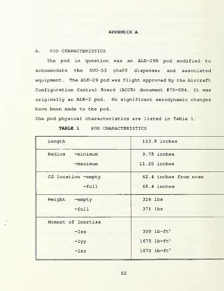
APPENDIX A

A. POD CHARACTERISTICS

The pod in question was an ALE-29B pod modified to

accommodate the SUU-53 chaff dispenser and associated

equipment. The ALE-2 9 pod was flight approved by the Aircraft

Configuration Control Board (ACCB) document #75-004. It was

originally an ALE-2 pod. No significant aerodynamic changes

have been made to the pod.

The pod physical characteristics are listed in Table 1.

TABLE 1 POD CHARACTERISTICS

Length 153. 8 inches

Radius -minimum 9.75 inches

-maximum 11.20 inches

CG location -empty 62.4 inches from nose

-full 65.4 inches

Weight -empty 326 lbs

-full 371 lbs

Moment of Inertias

-Ixx 300 lb-ft 2

-Iyy 1675 lb-ft 2

-Izz 1675 lb-ft 2

52

APPENDIX B

A. FORCE EQUATIONS

IF = M*V - d/dt (M*V) = G

Separating variables

IF X = G x lFy

= Gy

IFZ

= G z

Assuming £Fxy = 0,

Integrating the remaining equation,

JlF z dt = G 2- Gj = (M*V

Z ) 2- (M*V2 )i

Assuming straight and level flight, V zl= yields:

JlF z dt = M*AVZ

= M*VZ

Integrating the ejector force polynomial yields a total

impulse of 345 lb f-secs. Substituting (wt=371 lb),

345 lbf .secs = 371 lbm

* Vz

V z= 1.1773 (lb

f-sec/lbm )

* 32.174 (lbm-ft/lb f-sec 2

)

V z= 2 9.9 fps

53

B. MOMENT EQUATIONS

IM = r x IF = r x M*V = d/dt(r x M*V) = H

where H is the angular momentum about pt 0. Integrating the

moments,

JlM dt = H + r x H

Separating the component equations yields,

£MX = I xx *d)x - (Iyy

- I zz )*0)y *COz

ZMy

= Iyy*^ - (I„ - I xx ) *G)Z *CDX

IM Z= I zz *d)z

- (I xx - Iyy ) *caK *COy

Assuming the reference frame coincides with the principal

axes, I xy , xz , yz= 0, and assuming coxz = 0, yields the following:

JlMydt = I

yy* (by

toy =1.12 rad/sec

54

APPENDIX C

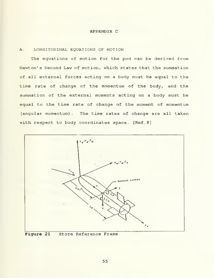
A. LONGITUDINAL EQUATIONS OF MOTION

The equations of motion for the pod can be derived from

Newton' s Second Law of motion, which states that the summation

of all external forces acting on a body must be equal to the

time rate of change of the momentum of the body, and the

summation of the external moments acting on a body must be

equal to the time rate of change of the moment of momentum

(angular momentum) . The time rates of change are all taken

with respect to body coordinates space. [Ref.8]

w ,c%1

y.. v .- cY

Figure 21 Store Reference Frame

55

£ AFx =/7?* (U+W*Q-V*R)

Y^ AFz=/7?* (W+V*P-U*Q)

£ &M=Q*Iy+ P*R* ilx"lg)

+ iP'-R 2) *JX

£ AFx=m* (C/+^*(?-V*i2)

£ AF2= m* (^+V*P-(7*0)

£AM=£)*Jy

By restricting the disturbances to small perturbations

about the equilibrium condition, the product of the variations

will be small in comparison with the variations and can be

neglected, and the small angle assumptions can be made

relative to the angles between the equilibrium and disturbed

axes .

J^ AFx=/n*ti

J^ AFz=m* (w-U*q) =m* (w-U*&)

£ AM=Iy*g=Iy *fc

Expanding the applied forces and moments in terms of the

changes in the aerodynamic and gravitation forces and moments

using the total differential form yields:

56

£ dFx= (dFjdu) *dl T+ (dFx/dw) *dw+ (dFx/dW) *dw+ (dFx/dG) *dS- {dFx/db[

£ dFz= idFjdu) *du+ (dFjdW) *dfV- {dFjdw) *dw+ (dF

z/d&) *dO~ (dFz/db[

Y, AM= idM/dU) *dU+ (dM/dW) *dW+ {dM/dW) *dW+ {dM/d&) *d&

Non-dimensionalizing the terms in the above equations

yield the aerodynamic coefficients. Following are the

definitions of the longitudinal stability coefficients and

derivatives

:

C xu Variation of drag and thrust with u.

C xa Lift and drag variations along the x-axis

.

Cw Gravity

C x(i Downwash lag on drag.

Cxq Effect of pitch rate on drag.

C zu Variation of normal force with u.

C xa Slope of the normal force curve.

Cxi Downwash lag on lift of tail.

C zq Effect of pitch rate on lift.

Cmu Effects of thrust, slipstream, and flexibility.

Cma Static longitudinal stability.

Cm<i Downwash lag on moment

.

Cmq Damping in pitch.

Arranging the linearized longitudinal equations into

matrix form yields the following matrix equation. The control

57

matrix B is not shown here but is included in the Control-C

program. Since there are no active control surfaces, the B-

raatrix is a zero matrix.

Au xu x. -g Au

Aw Zu Zw u Aw

Aq = MU+M„*Z U MW+MW*Z W Mq+M„*U Aq

AO. Ae

58

B. LATERAL EQUATIONS OF MOTION

In the same manner used to obtain the longitudinal

equations, the lateral equations are derived. The same

assumptions using perturbation theory apply. Following are

the equations in their developing order.

£ AFy=/77* ( V+U*R-W*P)

£ AL=P*IX-R*JXZ +Q*R* UM~Iy ) ~P*Q*JXZ£ AN=R*I

Z+P*JXZ +P*Q* (I

y-Ix ) +Q*R*JXZ

^T Afr=m* ( v+U*r+u*r)

Y,*N=r*I z-p*Jxz

^2 AFy=/77* ( v+U*r)

J2&L=p*Ix-r*JxzY;*N=r*I2-p*Jxz

£ dFy= {dFy/dB) *dB+ (dF

y/dlf) *dT+OFy/3*) *d«+ (8Fy/6$) *d*- (dF

y/-

Ap Yp/u Y

p/u -(l-Yr/u) g*cos0/u Af

Ap Lp

Lp

Lr Ap

Ar = Np

Np

Nr Ar

A<t> L1 A(D.

59

APPENDIX D

m- Input (' ente r m ( lbs ):

'

)/3 2 . 2

;

Uo-lnput ( ' ente r Uo (fpB)t')rS-input( 'enter S ( i n* * 2 )

t

*

)

/l 4

4

;

b-inpuM 'entet b (ln);')/12;Ro-lnput( 'enter Ro ( slugs/ft ** 3 ) t ') ;

cref-lnput (' enter c rtf I in )i

' J/12

;

Ix-input( 'enter Ixx ( ft-lb) j' )/32. 2|

Iy-input( 'enter IYY (

f

t-lb )i

' )/32 . 2

;

Iz-lnput( 'enter Izi ( ft-lb) t • )/32 . 2

|

g-32.174;Cn-lnput (' enter Cn (Normal force coefficient)!');Cm-1 nput (' enter Cm (Pitching Moment Coeff lclent ) I ' ) |

Ca-lnput (' enter Ca (Axial Force Coefficient)!'))Cy-tnput (' enter Cy (Side rorce Coefficient )

t' )

;

CLN-lnput( ' enter CLN (Yawing Moment Coeff):');CLL-lnput( ' enter CLL (Boiling Moment Coeff);');CNA-lnput (' enter CNA (Normal force Derlv wet AOA):');CMA-lnput (' enter CMA (Pitching Moment Derlv wrt AOA )

t' )

;

CYB-input( ' enter CYB (Side Force Derlv wrt Beta);');CLNB-lnput( ' enter CLN8 (yawing Moment derlv wrt Beta);');CLLB-lnput( ' enter CLLB (Rolling Moment deriv wrt Beta);');CL-input( 'enter CI (lift coeff);');CD-Input (' enter Cd (Drag coeff);');CNQ-lnput( 'enter CNQ (Normal Force Deriv wrt Q) ; '

) ;

CMQ-lnput( 'enter CMQ (Pitching Moment Derlv wrt 0);');CNAOADOT-lnput( 'enter CN AOAdot (Normal Force Derlv wrt AOAdot);');CMAOADOT-lnput( 'enter CM AOAdot (Pitching Mom Deriv wrt AOAdot);');q- . 5* ro*uo*uo;Xu--2*Cd*q*s/(m*uo) ;

Xw-Cl*q*s/(m*uo) ;

Zu

—

2*Cl*q*s/(m*uo) ;

Zw--Cd*q*s/(m*uo )

;

Zwd-Cnaoadot*cref*a*q/(2*uo»uo*m);Mw-Cma*q*B*cref/( Iy*uo) ;

Mu-0;Ma-uo*Mw;Mwd-Cmaoadot *cref *q*a*cre f/(2*uo*uo*Iy);Mad-uo*Mwd;Mq-Cmq*cref *q*S*cref/( 2*uo* Iy )

;

A-(Xu Xw -g;Zu Zw uo 0; ( Mu+Mwd*Zu )/( 1-Zwd ) ( Mw*Mwd*Zw)/( 1-Zwd) . .

.

(Mq+Mwd*uo)/( 1-Zwd) 0;0 1 0);B-(0 OjO 0J';C-10 1 0);D-[0 0);1C-10 0)' ;

IC(2)-input( 'enter initial vertical velocity (fps);');IC( 3)-input< 'enter initial pitching rate (rad/s);');ttt-input( ' enter end time (sec)');t-0; .001ittt|uuu-(ttt/.001)+l>u-0'ones ( 2 , uuu

)

;

simu( ' IC , IC) ;

y-slmu(a,br c,d,u,t) ;

erase ;

plot(t.y);

Figure 22 Control-C Program For EOM Simulation

60

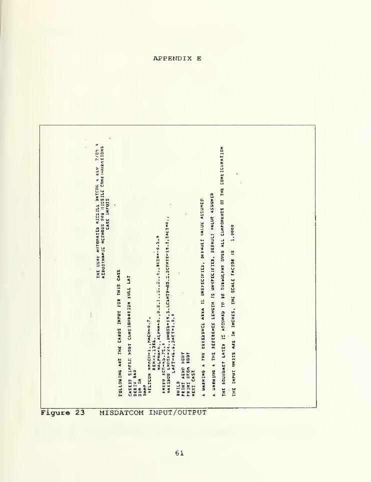
APPENDIX E

*r

•

VI rJ< X ou o •-•

X " *r* H «

c atat 3

:> r oM Iit — .k,

•

u. X« X oc ux oe UlUi Ul X- -I O ft*

« •"• Ula en in a c Uft

11 * Ul 3 oui ~« 3 c in-i = L. 3 VI inZ 1.1 < Hu ati r » « hi 5ft* u. Ul t 3 zc VI o M -i o

v> « • 3 < «- oa a «J H » c oui o * « 3 ei- X < 1> ft* u e« y M .Jc u ft M 3 -Io c .1 n -1 « -I»- 3 •m «- u o »< « U« ft*

1 a a » inc • > ai

Ml « c H a 3« X H H a O a*» S: X M o3 Q « K a ft* H M9 U uj u. X uw « 1*1 • a fit <x w VI *- » U _| Ul- « o

I/I

*<-1 11 n

?

UUl».

Ul•ft

v>X

3a*3

Ul

«-1 in 3 »* UX -J fl M X «n

»- 3 i H .

X3 in Ul

a Ul« ^ M 11 Xo X • (J X c *Ui O u -I

« 13»*

^

y> - o <n iJ X a VI3 < • • • at Ul K Ula. X. o» • « _l r XZ ~

t* <3 M O uft* o • 1 I • M V4 Ul X

<-* Q < * -• U U V.wt IftJ 1 X V) • X X «a X X X o »- Ul Ul Xat 3 u -1 X <-

3M It ft*

« u « < a « Ulo c sO • • a aw u> Ul

V- • M • » . . M ul M aui a • n c » V *» JU « Ul «X O -4 r* I al .•« 1 ft-

t- X I < ^ I J) *• ft- J* ul « VIT z • J. T a a X X -1 H

ui £j u 1 a. n m • o o ft* f* ft*

a ». c X -1 * 6 H X m >- X< L. r U < 1 X M hi < u 3

C z * z e -» « c c «~* a u J X o ui 19 o a H

X i/i « z x a u u. V) X 3ft* a o o « O < »* ft* 3 •.3 c X u o a o X X o Xo ft* » * M U. * a * ft- •• t. a_l u aa • -1 W X -J X Z * « «_l W a E C la K « •* ft* ft* X 3 3 hi . Ulo « U — « - • « 3 a a u X Xtu u a a a a a. «- z 41 *r a* a*

Figure 23 MISDATCOM INPUT/OUTPUT

61

n

u u</> a•t «

it. a.<J a.

*

•-

WI*oX

Xooeb*

ri

<

n-it

biV)oX

Xa

ooo10

ooCDT>

T

oo

en

fl o o& o m*o « ri

X X z z Z X oeOOoo

•Jl o on o oO --o n -< r> ori .1 * ^ ts. nen o •* en en nM o- »

-1 o r« en CD J CD* o r* en rt fl r**-• o a> o -o CD in o o o © oo*-

a» to ri o /i o o o co © in

n n* r i o O » r»o *]

CDCD in r.en -s f(

1 •» n n. O n sC1

1

t

" f* f*nn

^3 enri

urn

1 o o o en o ©o o o n o o

* o -1 a m m o(/>

* o —• PI S fl

fa

xo

>-

.3 u o tv n o V n* r> o O T* *

o en o CO o m<*.

JB Xa o

o0)r?

in•o

c09

eno r*

:>HIM

<*

-J

*-* o o o o O O ©o 'I r* n o Cf» cr» o o o o o o

Xa

f* o r* e? o o o ?OM•4, J 1

* —* di CD -• o *1 o *> -^

-«

r

Xa 3 •-•

1

1

1

;i o n- en #>

c z M<J <j X 3

I-j O 1 o o o o » o o<A •-

1

1

•-

z o o ©o s noo

en ii mi

- ^J >-1 o a r« » ri r. o

•1 C oO

>-

a m o tv e o u O o til

crCI

J en" JV) OB o w o -0 v o * r» e z*1 C m a o J> en o fl o oX O M X fl '• n -O en •i <o JE

Tou « w

j n n o J3 r* at a oooOoo 10 © ©

o o nMl1- X

t« far

XXMU

>•o a X en

o CD•*> .J

Oof 1 7* -^

r* *"> nfl fs en

xH OW X

X>• 1

r* r-- «:J

rfl en itf

o X v» 1N -n 13 (-1 J X %

*;X<

4. < o O O -. o oX o o o X © o1 o r ri en rt ©* in 1

1

m -3 n O r . en

=3 a 1 fal o CD a CD ri CO t^ 4 © J3 r> »» fv VIo 3- O ' O a r*> n |s. HM * itt o n «i o en r» zX Ul is. C9 o fl o ee o o f it-> 4 O o aX * ft n o o o O O © © o e.

1

1

n n.

oenenn o

onos0o

1-n © nft *t fi— r, to

V73Q

1 f 1 f« fl en eo 3n2 Z

a Ha < < z« a o o O O © o © © o

Vt u M o o c o o o © © U4 M a « H o o o o o r» /i o 1106 «X M

1* -*ZM

o o fl o ONM1QW X Z « U o < r* r» © en en ©

11 at w f i o %•» blX bl O u s u u A.

bl H itt Ul X X aa. O bl z « H 3 3 Wl j« z Z 1 •J H -> ~l X tnz bl -J M bt O o o aCA _J u* fl- < a 5 >

«

(A

-J

«X

aMoza-J

<m>-

ao

UlblV*

<(J

©z

«

1

biMOz

Figure 24 MISDATCOM Input/Output (Cont)

62

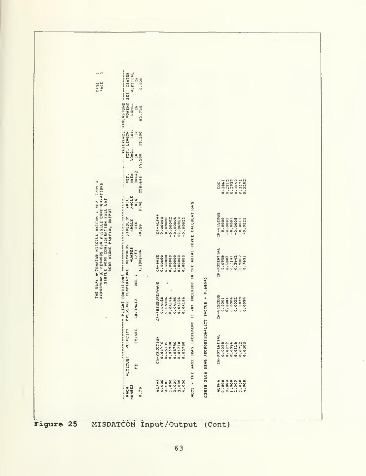
_ CI OC -1u «

z •-«

z oou (*i Ul M o

tn o U Of« * UJ ou *• • :>

Ul

ua

VI »-• •ZXO i oOU Z /»-co fs

l/> O -JZ c /I

ifl

c

a41 H x oU *• 4 oX 19 -J o-«- XAt Ul C*ti -i

jt • •

m m o11 z z oM 3 oJ

<•«

/l

J*

• « «tM Ul « 03Ul X z •r ^« UNM -• fl

ui

x o

Ot « tfl U sO — r» ,1 r- o>

o af 1

ceo — r i

M o o o o o o« UlJt H -J -4

> 3 < -J 13 u o tnU -1 a z a O zu •- at -t

U. -4 •-< o< Z -JO 3

C l-l .**

3ft.

H3a

a. X o — n 4 f tl

*-<

<x

JUl3C o —. *-» *-)

-* ui a. o o o o — n 3 (J o o o o — riUU1 -J -i tc kJ o 2 © o o o u -1 o © o © o oH»lQ ul o ijj 9 « O o O o o -1 o o o © o o<X »-• M _j u x o /I 1 o O o O O o <t >B'JIH <i O 4 -i o o © o © © ©

Ul 4 O U o o o o o o t 1 ) 1 1 1

-a -• jk u. tn 1 1 1 1 1 1 Ul o-J r 3 M U•"* C3 €(.1 M -« a. O

UiDI9 JH tr•- u* z itl a «n o Z -J u t~ -D jw u o o a u. 9 <ca a .J z c X o o o o o o H at r* «h m f• **y o >• < >• D Jl w o o o o o o M Z >n o * ** ** 0*>#-• X c ui z O c o o o o o o « a- CO «H J* CD ~D« v- o >• (M n X o o o o o o H o Hfin n r«C U X Q 1 o o o o o o M o3 X a « X © © © © O om Jig u (J o o o o © © MS U J « E* — ft. 1 3 M zc r ! : v* bl2tf « M ) « ID *«2|A * at '.U Ul Q o-1 !: I > ui O 9 jj 093 2 - ft. « 3 •4o i c a 3w <* ; : ta "N. kj ©X '< i ** Ul u V)** 4 i i Ot ti- 4 J> z 3 » -j ri a» ©

r* 3 cs cr co CO O CO O o ©on * 0"»• Ul « tn « U © © o © o ©

3 : ot 4 ^« O Ul o o o © o ©I I 3 Z w 3 o o o o © o V*« Ul oc z u > o o © o o oJ Ul a. o o o © © o « I

. Uloeft.

Hi-

uo

-I

Uw'.n

H

I

*j

zo

bi

*-•

zttl

X-J

Muz

u.

>~

zo

zCJ

-1

4-J u- o o o o © o 01 t-» X n>ia r* uui H c X u c z PI ."s C0 .1 r> ©> (_» r- fv r* fv tN o ft. u o o o -. ri n

D rt n r> /» *i € o M o o o o © ©0C o o o o o o * OB a

o © o o o ow 1 o o o © o © 1a « Ul o z3 t_> tl < (_)»"• H € at** |M X aM-1 fal 3< X

Ha

« o o o © o Ik € o O O O o ©X o o o o o o I o o o o o o« ft. o CD O © © © in A. o CO o © © ©

X W o -J Ul UlU ft) t-s 4 o o ~ ri n * M o « o O --II m *< r o «c 3 o Z uz

Figure 25 MISDATCOM Input /Output (Cont)

63

o o o o o Oi at -j1 Ul 4

X o— o _l

o o o o oUl Ul UJ jj Ulo © © o o

o

©Ul ui 1 UJ »-• o -1 O O O o o o(/» 19 1 1 . a» CJ o o © o o o4U •I 1 Ul

1 • ^o

_j o o © © © ©1 U* «1 Ul z1 JM oV) M • « © © © © o ©X X O z o (J +a ui z "• *1 JB Ul Ul Ul X Ul Ul~ x o r* « Z r --d -o * r i J3to o -J ff* ff^ 3s CT" ff" O)z cUl z

o U o o o o o oX 4 J

4 1a a CM

UJul x H z o H<-j t- « — o 1 © © © © © ©Ztf-« *i M J liltu z JOat Ul o« O. >• O O' !• D OUl -1 CJ •r> -o t i x —UiUJ • • VI

KI^MT 1 a

m ui oUl z z o

Ul1 1 1 1 1

1 31 3 — oto

3*4

© © © © ©,.rt Ul _i K n jiftH n x

1 • 4 * C 4 u s 0*1 CT1 a* X fs1 Ui Ul1 Ul «1 M <t

« az *

Z o o o o o o"

•> VIO3

<T* z u ao V*80 3 a» f 4 iA O O r<H r* (S p> «jj e * o* ©r* l-«

4V»

1 Ulzo

© © © © ©1 1 1 1 1

O1 u

ri n o ff» ^ n-» »- OK 1 -J -1 13 _l 4 '*l Ul Jj Ul i.' ul 1 * n n -• o 3*

3 3 <t UJ 1 -1 D Ul O Z J» — r o- j> * M m ri M ri f i ^V O -J •-• 1 O X a o (_> n a c © o .1at U 1 m i 'A N o 4 n o« X

-4 <-J M

o© O F* /l »• » "»*• * n a-i o rs.a 3 4 '_) © irt \J> n f i ^x (_) «* X i a. N OOOMfino (J 1 -* Ul -1u Ul X I J -i u> *J © © © © o ©

V- -J O (J 1 (.1 O Ul o« t Ul X o O 1a M C

« 4I a 4

o1

1w 0( z 1 V* I o o o o © © © © © e -• wpj i: 2 — -1 o o © o o o O o © o o o oa a 4 -1 o o © o o o un j» •- o Z -1crt a lu *1 i in 3 U © © o o o o © o © © © ©

X U| i a me

0)

o 4u

1 mm Ut1 C «

a u 1 Z X X Ulu o >- -•1 J- 3 -. UJ on ifl t0 sfl i0 in o © rt n9 * ,-> r«X © M 1 Ul Z e 0* 0> T1 3* C 3> J © © o ~* .-• n€ H 3 « 1 M m a Z © o o o o O LI o o o o © o

x Ul a i-CI *J j © © o © o ©o © o © © OH I Ul 4o -J ui en at

4£.

ft. Xx a

W 3X >-

M Ul

Ui C M _| O 4 13 4 * -r * rt O 4 © o o © © o< z (/) 4 ** J* Ul © © © o o © X o x © o o oVI >- H U. a >- © o o o o O a.3 a *U 0. 1 o -r © o +* tt r» ^a a a x 1 © © © o © © 4Ul at a X ui 1

X Ul a mM 4

V- ul

x atO 3

44z

© © o o o ««Ui Ul a o o © © o s>M 4 o

1 X1

1 -1

uo o o © o o

c »- U 41 M Ul Z1 ~* vt © n — n n1 U X. a © r> ff» co r» sG1 O1 -11 Ul

ou. £•X o -» -» rt n rv

o © o o © o1 >1

1

•DzO-J

1 X © JJ TO r- r* <ri a o o © -* r* n1 31 M1 -*

Hhi

X o © © © o o© © © © o o

1 H1 J1 11

1

1 4 o o o o o oI m1 x wI u

X-1

on ooo oIN. © © ~* r • n *

1 « c 41 X 3 ©l X

*

'

Figure 26 MISDATC0M Input/Output (Cont)

64

5 2

Vt V- •

z z u z oo ui Z ~ *1— CO ISIS) O -I •

z z nUl U)

JJ I M Z O(_) I- < ~ oZ 13 — *1- z

o o

«:• 3 -i w4i — >« I -J »-

u z z o

Ui Ul •« 00Ul jt Z Vat a "~

I I I | t

HI jj Ul J W |

o .i n -. rii

.o ^ r i — <rp* r» ff» v *

,

ts (p ^ a o|

W or* o n o .

r -p T

1/1 (J? W oUl z o «a 1 I

a 'il il U rfl U Ul« ^ O1 n f i .j j> .?•

u-Z ^ /> f I .i ?J *a. ._» T» o -* ri n m

If r c« C3 «

c i J> — Z- » C * »-

~ u, Z oc o

Wl -} Ula a zui o >- a<- i 3 -j« w o *CUT,a z »•- iia- u _j o•r — a. x

* C.*- a —< x tnM »-

-i (d H 4O A U* O

tfl 3Z *"•

a *

o o o o o ou o o o © © o-• »*CO Ul X 'il 41 u> J« Z ' X ^HN Jz (j * m o* -*i *r .s>- o ~+ r r ft oo -•

ft ri n <» ri vn

-J t/1

U. Ulo a> o o o oo o -* r i n *

X Ul oU A r-I c •

C 3 o

Figure 27 MISDATCOM Input/Output (Cont)

65

LIST OF REFERENCES

1. Mendenhall, M.R., Lesieutre, D.J., Caruso, S.C.,Dillinius, M.F.E., Kuhn, G.D., Aerodynamic Design of Pegasus,CP-4 93, paper presented at the AGARD Conference Proceedings#493, pages 7-1,2.

2. Air Force Flight Dynamics Laboratory, AFWAL-TR-8 6-30 91,Missile Datcom, Volume I- Final Report, Vukelich, S.R., Stoy,S.L., Bruns, K.A., Castillo, J. A., Moore, M.E., December 1988.

3. Air Force Flight Dynamics Laboratory, Technical ReportAFFDL-TR-72-83, Vol. I, 1972, Prediction of the Six-Degree-of-Freedom Store Separation Trajectories at Speeds up to theCritical Speed, Vol. I—Theoretical methods and Comparisonswith Experiment, by Dillenius, M.F.E., Goodwin, F.K., andNielsen, J.N., 1972.

4. Joint Ordnance Commander Subgroup For Aircraft/StoresCompatibility, AOP-12, Volume 3, Aircraft Stores InterfaceManual, pp. 2-(15-18), April, 1983.

5. CricketGraph* software, copyright 1990, ComputerAssociates

.

6. Nelson, R.C., Flight Stability and Automatic Control, page113, McGraw-Hill Book Co., 1989.

7. Dickenson, B., Aircraft Stability and Control for Pilotsand Engineers, p. 14, Pitman Publishing Corporation, 1968.

8. PC-MATLAB Version 3.2-PC software, copyright 1987, TheMathWorks, Inc.

9. Ctrl-C software, copyright 1986, Systems ControlTechnology, Inc.

10. Spahr, H. R. , Theoretical Store Separation Analysis of aPrototype Store, Journal of Aircraft, Volume 12, Number 10,page 807, October 1975.

11. van den Broek, G. J., The Use of a Panel Method in thePrediction of External Store Separation, Journal of Aircraft,Volume 21, Number 5, page 309, May 1984.

12. Miranda, L. R. , Extended Applications of the VortexLattice Method, Vortex Lattice Utilization, NASA SP-405, page27, 1984.

66

13. Bertin, J. J., Smith, M. L . , Aerodynamics for Engineers,Prentice-Hall, Incorporated, 1989.

67

INITIAL DISTRIBUTION LISTNo . Copies

1

.

Defense Technical Information Center 2

Cameron StationAlexandria, VA 22304-6145

2. Library, Code 52 2

Naval Postgraduate SchoolMonterey, CA 93943-5002

3

.

Chairman 1

Department of Aeronautics and AstronauticsNaval Postgraduate SchoolMonterey, CA 93943-5000

4

.

Commander 1

Pacific Missile Test CenterPoint Mugu, CA 93042

5

.

Naval Air Systems Command 1

AIR-530EWashington, D.C. 20361

6. Flight Dynamics Laboratory 1

Air Force Wright Aeronautical LaboratoriesAir Force Systems CommandATTN: Mr. William BlakeWright Patterson Air Force Base, OH 45433-6553

7

.

Naval Weapons Center 1

Code 3592ATTN: Mr. L. GleasonChina Lake, CA 93555

8

.

Pacific Missile Test Center 4

Code 9053Point Mugu, CA 93042

9. Prof. 0. Biblarz, Code AA/Bi 1

Department of Aeronautics and AstronauticsNaval Postgraduate SchoolMonterey, CA 93942-5000

10. Prof. L. Schmidt, Code AA/Si 1

Department of Aeronautics and AstronauticsNaval Postgraduate SchoolMonterey, CA 93942-5000

68

ThesisH201235 Hansen

I

l Store separation

methodology analysis,

TherisH201235 Hansenc.l Store separation

methodology analysis