stock returns and real activity: a structural approach - european
TRANSCRIPT

EUROPEAN
K%!x?Mc ELSEVIER European Economic Review 39 (1995) 981-1015
Stock returns and real activity: A structural approach
Fabio CanovaaTbpc3 * , Gianni De Nicolo’ d7e
a Department of Economics, Universitat Pompeu Fabra, Balmes 132, E-08008, Barcelona, Spain b Dipartimento di Economia e Commercio, Uniuersid di Catania, I-95100 Catania, Italy and CEPR
’ CEPR, London, UK ’ Department of Economics, Brandeis University, Waltham, MA 02254-9110, USA
e Dipartimento di Scienze Economiche, Uniuersita di Roma ‘La Sapienza’, Via Cesalpino 12/14,
I-00161 Rome, Italy
Received July 1994, final version received February 1995
Abstract
This paper analyzes the relationship between stock returns and real activity from the
point of view of a general equilibrium, multicountry model of the business cycle. The empirical evidence suggests that there is a relationship between domestic output growth and domestic stock returns which becomes stronger when foreign influences are considered. We study the properties of a model with two sources of disturbances and three mechanisms of transmission across countries. We show that the model can best reproduce the actual data when technology shocks drive the cycle and when there is a common international component to the shocks. The strength of association between stock returns and output growth depends on how future expected cash flows respond to the disturbances. Intema- tional linkages emerge because foreign variables contain information about the future path of domestic variables.
Keywords: Transmission; Business cycles; International stock returns; Financial markets
JEL classification: C15; E43
* Corresponding author.
0014-2921/95/$09.50 0 1995 Elsevier Science B.V. Ah rights reserved SSDI 0014-2921(95)00017-8

982 F. Canova, G. De Nicolo’/European Economic Review 39 (1995) 981-101.5
1. Introduction
Richard Roll (1988) in his presidential address to the AFA suggested that
“The immatnrity of our science is illustrated by the conspicuous lack of predictive content about some of its most interesting phenomena, particularly, changes in asset prices.”
In response to this challenge a number of authors, including Roll (1988), Fama
(19901, Schwert (19901, Cutler et al. (1989), Bekaert and Hodrick (1992) and Campbell and Ammer (19931, have tried to explain asset price changes using news events or proxies for expected returns and future cash flows. The approaches employed differ - some authors use aggregate stock market data in isolation while others use it in conjunction with other financial market data, such as bonds or
foreign exchange data. Moreover, some employ only contemporaneous informa- tion to predict asset price changes while others use leads of informational variables
as an informal way to allow for extra information that agents may have about future macroeconomic developments.
The simple contemporaneous regression or unrestricted VAR frameworks used
to explain asset price variability are appealing because of their simplicity, but they have little to say about more structural questions. For example, the techniques do not explicitly allow us to identify which source of disturbance is most likely to
drive asset price changes (e.g., demand or supply disturbances), nor the channels through which news affects, on one hand, the right-hand side variables of the regression used to explain asset price variability, and, on the other, asset prices themselves.
One way to tackle this problem is to build explicit behavioral models where the sources and propagation mechanisms can be clearly identified and examine whether the reduced form evidence they produce is consistent with the reduced
form evidence available in the actual data. This is the approach taken by e.g., Balvers et al. (19901, Rowenhorst (19911, Jermann (19941, Danthine and Donald- son (1994) and Canova and Marrinan (1995) which use general equilibrium models to interpret moments of the data and the predictability of excess returns in
various domestic and international markets. Another strand of literature, pioneered by Burns and Mitchell (19431, attempts
to predict changes in real activity using a set of leading indicators. Recent contributions by Stock and Watson (19891, Jeager (1991) and Plosser and Rowen- horst (1994) indicate that some financial variables, in particular term spreads, default spreads and stock returns, lead turning points of real activity and capture future developments of the real side of the economy. However, this literature also faces the same problems encountered by the previous one: because the exercise is statistical, structural questions concerning what induces financial variables to lead real activity and through what channels can not be asked.

F. Canova, G. De Nicolo ‘/ European Economic Review 39 (1995) 981-1015 983
In this paper we combine these two branches of literature within a structural
approach in order to provide some rationale for the otherwise uninterpretable reduced form evidence. We consider the relationship between asset returns and real activity within a general equilibrium model where there are multiple sources of shocks and multiple channels of domestic and international transmission. This type of model can be used to address three crucial questions: (a) what kind of shocks contribute to move both asset returns and real activity; (b) which channel of transmission links domestic financial markets and domestic real activity and (c) what international linkages are necessary to generate the relationship between asset returns and real activity we observe in international data.
The model we employ is similar to Canova (1993). It features three countries,
two types of disturbances and two sources of international interdependencies (trade in intermediate goods and final consumption goods). One type of distur- bance we consider takes the form of exogenous government expenditure shocks
(as e.g. in Christian0 and Eichenbaum (1992)). These shocks leave the instanta- neous marginal product of factors of production unchanged but generate dynamic responses of outputs and asset prices because they modify intertemporal labor supply decisions of domestic households, the expected cash flows accruing to stockholders and their discount factors. A second type of disturbance is modelled as exogenous technology disturbances, as is standard in the real business cycle literature. These shocks instantaneously affect the marginal product of factors of production, have a direct influence on investment opportunities and cash flows and an indirect influence on consumption and asset prices because of permanent income considerations. Although these two types of shocks imply different
cyclical behavior for several variables of the model, for the purposes of this paper the crucial difference is in the way they impact on dividend payments and on the pricing kernel. With government shocks dividends and asset prices are strongly
procyclical. With technology shocks dividends and asset prices are weakly coun- tercyclical or acyclical.
The framework of analysis employed differs from both the simple domestic business cycle models used by Balvers et al. (1990) Jermann (1994) or Danthine and Donaldson (1994) and the international real business cycle models existing in
the literature (see e.g. Mendoza, 1991; Backus et al., 1992; Baxter and Crucini, 1993; Stockman and Tesar, 1994) in several respects. First, each country special- izes in the production of one good while agents in each country consume an array of goods produced in various countries. This setup allows us to independently parameterize the dividend process of each country, a possibility which is not
available in one good models of the international business cycle. Second, prefer- ences and technologies are allowed to differ across countries. Heterogeneity may be a useful way to remedy well known failures of the versions of the consumption based CAPM and of the Q-theory of investment which are built into the model (see Constantinides and Duffie, 1992). Third, foreign capital goods are used in the production of domestic goods. Allowing for production interdependencies intro-

984 F. Canova, G. De Nicolo’/European Economic Review 39 (1995) 981-1015
duces a previously neglected channel through which idiosyncratic shocks may be propagated across countries.
We summarize the basic features of the relationship between output and stock returns using the same regression analysis popularized by Fama (1990) and
Schwert (1990). Fama concludes that real activity and stock returns are related by showing that proxies for shocks to future cash flows, time variation and shocks to discount rates explain about 59% of annual stock returns variability in the US. We examine the relationship between domestic output growth, stock returns and dividend yields using three-month returns for the period 1973-1991 for five
different countries, the US, the UK, Germany, France and Italy and for an aggregate we call Europe with two goals in mind. First, we would like to know whether European economies conform to the pattern that researchers have found in the US. To the best of our knowledge, no one has yet documented whether there exists a relationship between stock returns and real activity for these economies and, if so, the strength of the association. Second, we would like to measure the relationship between real activity and stock returns when specific international
links are allowed (as e.g. in Harris and Opler (1990)). Although for the US economy external shocks may play a minor role over this period, European economies are more open to foreign disturbances and this may weaken the strength of the domestic association between stock returns and cyclical activity. If
this is the case, it is interesting to study whether a foreign indicator of cyclical activity may be useful to predict domestic stock returns and whether foreign
financial variables act as leading indicators for domestic activity. To complete the description of the properties of the data, we also present
selected unconditional second moments of the variables of interest. Our data suggest that the association between stock returns and growth rates of
production is as strong in some European countries and Europe as a whole as it is in the US, but there are also important cross-country and cross-continent differ- ences. In particular, lagged European stock returns explain both US and European GNP growth, while US stock returns are significant only in explaining European GNP growth. Moreover, future European GNP growth explains European stock returns, but the explanatory power of future US GNP for stock returns in both continents is weak. In addition, we find that the US dividend yield, a variable which is very important to explain stock returns in the US, has also some predictive power for stock returns in major European countries, whereas the European dividend yield has no predictive power.
We simulate various versions of the model under different economic scenarios. We compare the outcomes of the model to the actual data informally by presenting unconditional second moments and regression coefficients using calibrated param- eters and drawing one time path for the exogenous variables. To examine the incremental explanatory power of alternative specifications of the model we compactly summarize the reduced form evidence by reporting the mean and the
F. Canoua, G. De Nicolo’/European Economic Reuiew 39 (1995) 981-1015 985
standard deviation of the adjusted R* of the regressions constructed by randomiz- ing the exogenous processes of the economy.
Our basic findings can be summarized as follows. First, the model can produce
the type of association between domestic stock returns and domestic real activity we see in the data but, with unlevered equities, its strength depends on the source of disturbances driving the cycle. With levered equities this qualitative distinction
fades. When government expenditure shocks drive the international cycle the association between real GNP growth and stock returns is primarily due to the strong positive effect that these disturbances have on dividend payments. When
technology shocks drive the cycle, dividend yields are less correlated with GNP because the effect of disturbances on dividends and on expected future payoffs of the assets is tempered by the change in investments occurring in response to changes in the productivity of capital. Second, we also demonstrated that our model produces some of the important cross country spillovers between stock returns and real activity we see in the data and that all the three possible channels
of international transmission that the model displays are crucial in generating the type of cross country linkages we see in the actual data. Finally, we show that the introduction of asymmetries in the primitives of the model does not quantitatively
help to match the asymmetries displayed by the data, even though, qualitatively, the model’s outcomes change in the right direction.
The rest of the paper is organized as follows: the next section reports the
empirical evidence. Section 3 presents the model and Section 4 discusses some of its features. Section 5 presents the basic parameterization of the model. Section 6 contains the results. Section 7 concludes.
2. Some empirical evidence
In this section we document the strength of the relationship between stock returns and real activity using a set of regressions similar to those employed by Fama (1990) and Schwert (1990). We present two types of regressions: one where
only domestic factors are included and one where we attempt to capture intema- tional linkages between stock returns and real activity. For completeness, we also present selected unconditional second moments of the variables of interest.
Ideally, one would like to run VAR or multivariate systems in order to study the linkages between financial markets and real activity. It is well known that VARs can approximate arbitrarily well the joint unconditional distribution of the variables of interest while regression analysis does not. However, two reasons discourage us from pursuing this approach. First, because the sample is short and the number of variables potentially important is large, a VAR analysis is likely to produce either uninterpretable or statistically insignificant results. Second, because our task is to provide a rationale for reduced form evidence a la Fama, we would

986 F. Canova, G. De Nicolo’/European Economic Review 39 (1995) 981-1015
like to retain as much as possible Fama’s approach even though measurement errors and data problems may lead to a misspecification of the relationship.
The data set consists of quarterly data on real stock returns, dividend yields and
real GNP, consumption and investment for the US, the UK, France, Germany and Italy for the period 1970-1991. Stock returns and GNP data are obtained from OECD economic outlook, dividend yields data are obtained from Datastream.
Quarterly data are used to reduce the extent of measurement error in production data. This choice of sampling interval may reduce the information content of stock returns. However, Fama shows that the qualitative features of the relationship are not altered when monthly data are used with industrial production replacing GNP.
Therefore, examining quarterly data should suffice. We consider the evidence for each of the five countries and for an aggregate we
call Europe. Real stock returns for Europe are computed as an average of the four component countries’ stock market returns weighted by market capitalization in
1993 US$. Europe stock market dividends are computed as an average of component countries’ yields weighted by market capitalization. Because the relative shares of these markets in total are approximately constant over time, the results are invariant to the date chosen to index market capitalization. Europe real
variables are obtained by averaging real growth rates of the four component countries weighted by the fraction of real GNP for each country in the aggregate, evaluated in 1980 US$. Following Fama and French (1988), Fama (1990) and others, we use dividend yields as proxies for expected returns, and future real
GNPs, as proxies for shocks to expected future cash flows, in regressions with
stock returns as right-hand side variables. It is well know that other measures such as the term spread or the default
spread between high and lower grade corporate bonds are important in capturing information about business cycle conditions. However, because of difficulties in finding comparable measures for these spreads for all countries, we exclude them from the regressions. In addition, results of Fama and Schwert suggest that,
because these two variables are forward looking, they tend to loose their informa- tional power when future GNP growth is included in the regressions. Other variables which are known to be good indicators for real activity, such as the Federal Funds rate or housing starts, are not considered because they have no counterpart in the model of Section 3.
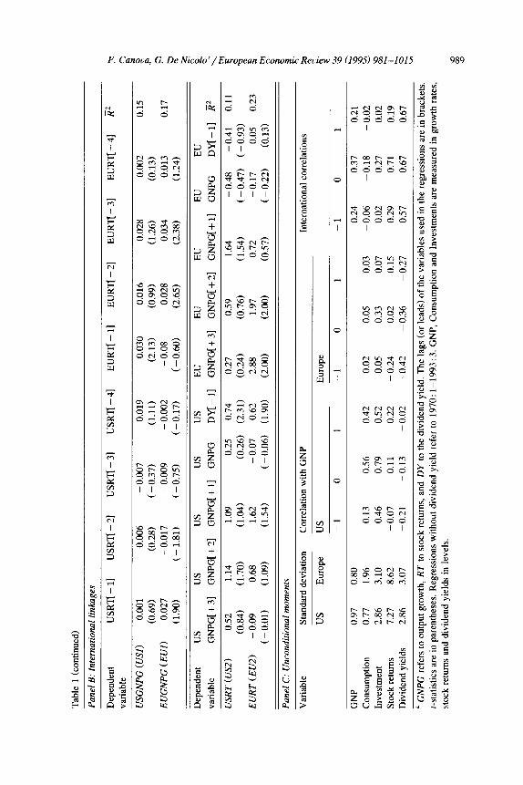
Table 1 contains our results. Panel A reports regression results obtained using a closed economy framework and panel B regressions results where some intema- tional influences are allowed. In each panel the first set of regressions with GNP as dependent variable and lagged stock returns as explanatory variables examines whether or not stock returns act as a leading indicator for real activity. In the second set of regressions we check whether lagged dividend yields and future GNP growths have any informational content for stock returns. Panel C contains measures of volatility and of domestic and international comovements for the variables of interest.

F. Canova, G. De Nicolo’/European Economic Review 39 (1995) 981-1015 987
There are several features of panel A which deserve attention. First, GNP
growth is predicted by at least one lagged return in the US, Germany, France and Europe, indicating some forward looking behavior of stock returns. The lack of predictive content of stock returns in the UK could be explained recalling that the value of national stock market is only partially a claim to national GNP as many stocks quoted in London are claims to foreign assets. Second, at least one
coefficient of future GNP growth is significant in predicting current stock returns in all countries except Italy. The adjusted R2 of both types of regression is higher
for aggregated Europe than for any of the four European countries and the US. Third, while the dividend yield explains stock returns in the US and in the UK, this is not the case in any of the other three countries and in Europe. The sign of the coefficient of dividend yield in all regressions, however, is consistent with the idea that expected returns are high when times have been poor (see e.g Fama,
1990). Fourth, the real and financial sides of the aggregate European economy closely track the real and financial sides of component economies but the association between stock returns and real activity for this aggregate appears to be stronger than for any of the individual European countries. For this reason, we consider Europe as a main block of interest in considering the interactions across
economies. Panel B indicates that there is additional explanatory power in foreign vari-
ables: the adjusted R2 of the regressions are larger here than in panel A, but the magnitude of the change is not dramatic. In addition the table shows several interesting asymmetries across the two continental blocks. First, in the regression with the US GNP growth as dependent variable, lagged European stock returns
become significant whereas the significance of lagged US stock returns wanes. On the other hand, stock returns in the US have some explanatory power for European GNP growth in addition to European stock returns. Second, the US dividend yield has predictive power for both the US and European stock returns, while the European dividend yield does not. Third, the point estimate of the contemporane- ous coefficient of domestic GNP growth in the stock return regressions is positive
for the US and negative for Europe. Note also that foreign future GNP growth does not seem to significantly affect domestic stock returns in both continental
blocks. Panel C shows that all variables are at least 2 to 3 times as volatile as output in
Europe, while in the US this is true for all variables but consumption. The correlation of European consumption with GNP is surprisingly low in our data set perhaps indicating the presence of measurement errors in consumption data for Europe. Stock returns are substantially more volatile than GNP in both continental blocks while dividend yields and investments have approximately the same variability. The domestic correlations indicate that dividend yields are counter- cyclical in both continents, even though the magnitude of the correlation is not very significant, and that stock returns are essentially acyclical. International correlations indicate that stock returns and dividend yields are more correlated

Tab
le 1
E
S
tock
ret
urn
, ou
tpu
t gro
wth
, di
vide
nd
yiel
d re
lati
onsh
ip a
Pan
el A
: In
diui
dual
ec
onom
ies
Dep
ende
nt
Rfl
-11
Rq-
21
Rfl
-31
Rfl
-41
GN
PG
[ + 3
1 G
NP
G[ +
21
GN
PG
[ + l
] G
NP
G
DY
[-11
R
2 3
vari
able
C
U
KG
NP
G
- 0.
005
0.00
1 0.
030
0.01
3 0.
01
B
C-0
.21)
(0
.53)
(1
.30)
“Q
(1
.31)
G
ER
GN
PG
9
- 0.
013
0.04
0 -
0.00
2 0.
032
0.05
2
(-
0.72
) (2
.50)
( -
0.2
2)
(2.0
4)
FR
AG
NP
G
- 0.
009
0.02
2 -
0.00
5 0.
003
2 0.
04
fi’
(-
1.28
) (2
.93)
(
- 0.
74)
(0.5
7)
%
ITA
GN
PG
0.
013
0.00
4 -
0.00
01
0.00
7 -0
.00
<
(1.2
8)
(0.6
1)
C-0
.13)
(1
.12)
P
a
US
GN
PG
(RI)
0.
026
0.03
3 ?i
0.
065
0.01
6 0.
09
3 (1
.68)
(2
.05)
(0
.49)
(1
.48)
E
IJG
NP
G (R
2)
0.00
8 0.
018
0.03
0 0.
011
0.16
R
(0.8
2)
(2.4
8)
$ (2
.57)
(1
.44)
8.
VK
RT
3.
30
1.11
1.
31
1.03
0.
31
:
(2.8
6)
(1.4
3)
(%
(1.4
3)
(3.4
8)
8.
GE
RR
T
0.98
1.
27
0.26
0.
62
0.25
0.
01
9
(1.7
2)
(2.2
2)
(0.3
7)
(0.8
5)
(0.5
9)
%
FR
AR
T
0.07
4.
23
- 1.
05
- 1.
01
0.31
0.
02
;:
(0.0
5)
(2.7
5)
(-0.
51)
( - 0
.99)
(1
.02)
z!
%
ITA
RT
0.
42
1.72
1.
11
0.12
-
0.03
(%
Z,
5 (0
.30)
(1
.02)
(0
.71)
(0
.24)
I
US
RT
(R3)
2
0.25
1.
35
0.55
0.
46
0.12
C
(0
.38)
&
(1
.41)
(0
.62)
(2
.01)
E
UR
T
(R4)
3.
41
2.49
1.
63
0.35
0.
58
0.22
(2.7
3)
(2.3
6)
(1.0
1)
(0.7
5)
(1.6
2)
F. Canoua. C. De Nicolo’/European Economic Review 39 (1995) 981-1015

990 F. Canova, G. De Nicolo’/European Economic Review 39 (1995) 981-1015
than outputs, suggesting the presence of either high financial capital mobility or common financial shocks. Finally, note the strong persistence of the international correlation of dividend yields. These qualitative features persist when UK or
German variables are used in place of European ones but the European economy as a whole interacts in a much stronger and interesting way with the US economy than any of the four individual economies taken separately.
To summarize, the reduced form evidence exhibits the following features: 0 For both continental blocks domestic stock returns lead real activity and future
domestic GNP growth has some informational content for stock returns. The
lagged dividend yields contain information about stock returns only in the US. 0 The strength of the association between stock returns and real activity increases
when international influences are allowed. 0 There are asymmetries between Europe and the US. In particular, (i) the US
dividend yield predicts both US and European stock returns whereas European dividend yield does not, (ii) European stock returns are significant in US GNP
regressions (making domestic stock returns insignificant) while US stock returns are significant in European GNP regressions in addition to European stock returns.
0 All variables but consumption in the US appear to be more volatile than output. In particular, the variability of stock returns in both continents is larger relative to the variability of GNP and the variability of dividend yields and investments is approximately the same.
0 Dividend yields are countercyclical and stock returns acyclical. In general, the correlation of financial variables with GNP is low. In addition stock returns and
dividend yields are more highly correlated across countries than GNP.
3. The model
The model we employ is similar to Canova’s (1993). It is a three-country model
with three consumption goods and each country specializing in the production of one good. We consider three ‘countries’ (say, US, Europe and the Rest of the World (ROW)) in order to maintain comparability with the empirical exercises of Section 2 where the two continental blocks we consider are only a part of a world economy.
The model abstracts from money, not because we believe that monetary aspects are unimportant in generating or transmitting business cycles to financial markets, but because we do not have simple general equilibrium models of money which can produce quantitatively interesting real cyclical effects (see e.g. Danthine and Donaldson, 1986).

F. Canova, G. De Nicolo’ / European Economic Review 39 (1995) 981-1015 991
Each country is populated by a large number of identical agents and labor is
immobile across countries. Preferences of the representative agent of country h = 1, 2, 3 are given by
(1)
where chjt is the consumption of good j by the representative agent of country h at time t. Agents value the services of up to three consumption goods: if good j is
not enjoyed by residents of country h, 8,j = 0. Consumption goods are produced according to the technology
Yhr =A,,, fiK$,~ ( XhtNhl)l-E:=lah~ i I
Vh, i, j=l
(2)
where X,,, = -y,,X,,_ 1 with y,, > 1 Vh represents a labor-augmenting Hicks-neu- tral deterministic technological progress. Production requires domestic labor and up to three intermediate capital inputs and is subject to a technological disturbance
All,. If intermediate input of country j is not used in producing the output of country h, ahj = 0. Capital goods are accumulated according to
&jr+ 1 = (1 - ‘j)K/zjt + 4hj( ‘hjt/Kh,t)Kh,r Vh, .i, (3)
where I+!J~~(Z~~,/K~ jt) satisfies I,!+,, > 0, I);~ > 0, I,$,‘~ G 0 for all h, j, and repre- sents the cost of installing (or moving) intermediate capital good j from the location where it is produced to country h.
Mendoza (19911, Backus et al. (1992) and Baxter and Crucini (19931 have shown that in a one good model of the international business cycle installation costs help to avoid unrealistic unidirectional capital flights in response to produc-
tivity disturbances. In this model unidirectional capital flights need not occur because of production interdependencies. Investments in the capital good produced in the country experiencing a positive productivity disturbance increase but there
may also be a contemporaneous flow in the opposite direction as investments in the other capital goods increase with the wealth of the country. However, the size of these flows may be very large in both directions and installation costs may help
to produce a more realistic variability of total investment across countries. The formulation adopted here extends that of Baxter and Crucini (1993) by allowing for asymmetric adjustment costs, and is chosen because it retains simplicity, while linking adjustment costs to Tobin’s Q. l/$’ is in fact Tobin’s Q, i.e. the price of existing capital in location h relative to the price of new capital imported from
location j. Note that absent adjustment costs Tobin’s Q is identically equal to one for all t and this closely ties together the returns to physical capital and to financial investments (see e.g. Danthine and Donaldson, 1994).
Leisure choices are constrained by
O<l,,+N,,<l Vh, (4)
992 F. Canova, G. De Nicolo’/European Economic Review 39 (1995) 981-1015
where we normalize the total endowment of time in each country to be equal to 1 for all 1.
To ensure that a balanced growth path with a stationary distribution of wealth
obtains we assume that p = p,,‘~,, and that y = yh p,, Vh where p,, is the growth rate of population in country h. Intuitively these conditions imply that, asymptoti- cally, the more impatient country will not accumulate all of the world wealth.
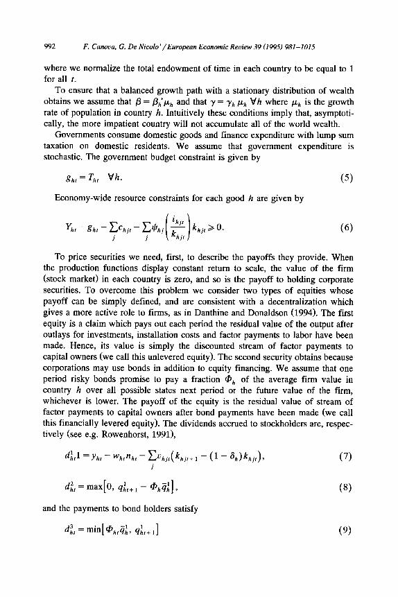
Governments consume domestic goods and finance expenditure with lump sum taxation on domestic residents. We assume that government expenditure is stochastic. The government budget constraint is given by
gh, = Tht Vh.
Economy-wide resource constraints for each good h are given by
yht - gh, - &hjr - &,j kh, > 0.
i j
(5)
(6)
To price securities we need, first, to describe the payoffs they provide. When the production functions display constant return to scale, the value of the firm (stock market) in each country is zero, and so is the payoff to holding corporate
securities. To overcome this problem we consider two types of equities whose payoff can be simply defined, and are consistent with a decentralization which gives a more active role to firms, as in Danthine and Donaldson (1994). The first
equity is a claim which pays out each period the residual value of the output after outlays for investments, installation costs and factor payments to labor have been made. Hence, its value is simply the discounted stream of factor payments to capital owners (we call this unlevered equity). The second security obtains because
corporations may use bonds in addition to equity financing. We assume that one period risky bonds promise to pay a fraction Gh of the average firm value in country h over all possible states next period or the future value of the firm, whichever is lower. The payoff of the equity is the residual value of stream of factor payments to capital owners after bond payments have been made (we call this financially levered equity). The dividends accrued to stockholders are, respec- tively (see e.g. Rowenhorst, 1991),
dial = Yhr - Whrnhr - CUhjt(khjt+l - t1 - 6h)khjt)j (7)
d;, = max[O, 41ft+ 1 - @,,q;] ,
and the payments to bond holders satisfy
F. Canova, G. De Nicolo’/ European Economic Review 39 (1995) 981-l 015 993
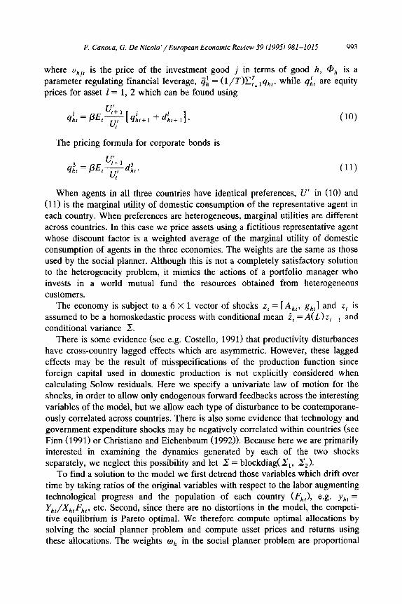
where uhjt is the price of the investment good j in terms of good h, ah is a
parameter regulating financial leverage, 4; = (l/TlXy= Iqht, while qit are equity prices for asset I = 1, 2 which can be found using
The pricing formula for corporate bonds is
U’ q;, = PE+d;,.
u: (11)
When agents in all three countries have identical preferences, U’ in (10) and (11) is the marginal utility of domestic consumption of the representative agent in each country. When preferences are heterogeneous, marginal utilities are different
across countries. In this case we price assets using a fictitious representative agent whose discount factor is a weighted average of the marginal utility of domestic consumption of agents in the three economies. The weights are the same as those used by the social planner. Although this is not a completely satisfactory solution to the heterogeneity problem, it mimics the actions of a portfolio manager who invests in a world mutual fund the resources obtained from heterogeneous
customers. The economy is subject to a 6 X 1 vector of shocks z, = [Ah!, gh,l and z, is
assumed to be a homoskedastic process with conditional mean f, = A(L)z,_~ , and conditional variance 2.
There is some evidence (see e.g. Costello, 1991) that productivity disturbances
have cross-country lagged effects which are asymmetric. However, these lagged effects may be the result of misspecifications of the production function since
foreign capital used in domestic production is not explicitly considered when calculating Solow residuals. Here we specify a univariate law of motion for the shocks, in order to allow only endogenous forward feedbacks across the interesting variables of the model, but we allow each type of disturbance to be contemporane-
ously correlated across countries. There is also some evidence that technology and government expenditure shocks may be negatively correlated within countries (see Finn (1991) or Christian0 and Eichenbaum (1992)). Because here we are primarily interested in examining the dynamics generated by each of the two shocks separately, we neglect this possibility and let _% = blockdiag(Z,, 2,).
To find a solution to the model we first detrend those variables which drift over time by taking ratios of the original variables with respect to the labor augmenting
technological progress and the population of each country (Fhrl, e.g. yh, = Y,,,/X,,,F,,,, etc. Second, since there are no distortions in the model, the competi- tive equilibrium is Pareto optimal. We therefore compute optimal allocations by solving the social planner problem and compute asset prices and returns using these allocations. The weights o,, in the social planner problem are proportional

994 F. Canova, G. De Nicolo ’ / European Economic Review 39 (I 995) 981-l 015
to the initial per-capita wealth of each of the three economic blocks. The optimality conditions are then approximated with a log-linear expansion around
the steady state as in King et al. (1988). Solutions for the variables of interest are computed analytically from the approximate optimality conditions.
It is feasible to construct a market structure which supports this planner’s problem (see e.g. Prescott and Mehra, 1980) and to give firms meaningful intertemporal decision problems. Danthine and Donaldson (1994) present an
ingenuous and simple way of doing so for a closed economy model. The extension of their approach to our open economy framework is straightforward. The only two additional assumptions that are required are that consumers can freely
purchase securities of all three countries (no capital controls are in place) and that firms freely trade capital goods at the price phjr.
With this model we will investigate three questions. First, we want to know under which generation mechanism (technology or government disturbances) the model comes closest to qualitatively reproducing the reduced form evidence In examining this question we will require that the data generated by the model does
not grossly violate the second moments of actual real and financial variables. Second, we want to study, under each generation mechanism, what are the channels inducing domestic and international comovements in stock returns and real activity. Third, we want to examine under each generation mechanism which channel of international transmission is crucial to allow foreign variables to add explanatory power to domestic regressions.
4. Discussion
The model we presented in Section 3 is sufficiently complex to make it
worthwhile to discuss why we need such a model for our purposes and what are the properties of the data that simpler frameworks can not explain. To do so we start by examining what one good models of the international business cycle tell us about the domestic and international stock return-real activity relationship.
4.1. One good model
4.1.1. Technology disturbances In a one good world with uncorrelated but persistent technology shocks, a
positive domestic disturbance raises the productivity of domestic factors, increases domestic investment, domestic output, domestic hours worked and, to a lesser extent, domestic consumption because of permanent income considerations. When installation costs are negligible, investment picks up the slack between production and consumption. Because of the one good assumption, capital flows to the most productive location (and the extent and the timing of this flow depend on the cost of installing capital) and induces a decline in investment, output and labor demand

F. Canova, G. De Nicolo’/ European Economic Review 39 (1995) 981-1015 99s
in the other countries. However, because of international risk sharing considera- tions, consumption profiles will be highly correlated across countries.
The effect of technology shocks on domestic equity prices depends on two contrasting factors: first, because output increases, firms’ earnings increase. Part of the increase will finance new investments (in the form of retained earnings) and
part will be distributed to shareholders (capital owners) in the form of increased dividend payments. In general, dividends payments will be only partially related to business cycle conditions since, unless installation costs are large, investment
increases to take advantage of the higher productivity of capital. In other words, we will observe some form of dividend smoothing over the business cycle. If shocks are persistent, future cash flows accruing to shareholders are expected to increase and this increases equity prices. The second effect comes about because
technology shocks influence consumption and hours decisions of agents and therefore the pricing kernels in the asset pricing equations. The direction and the magnitude of this effect depend on the persistence of the shocks. For highly
autocorrelated shocks, the pricing kernel is likely to decrease and this depresses asset prices. The strength of the domestic association between output growth, dividend yields and stock returns will therefore depend on the relative importance
of these two factors. Stock returns will be positively associated with current and future output growth if the effect of the disturbance on future cash flows is
stronger than the effect on the pricing kernel. In a model where agents are risk averse this is likely to be the case since the penalty for not smoothing consumption is large.
Future foreign output growth will help to predict domestic stock returns if it
carries information about future domestic output growth which is not entirely incorporated in domestic variables. For example, if future foreign output growth carries information about the extent of the feedbacks of technology disturbances, it
will be significant in the regressions with stock returns as right-hand side variable. However, because there is one good only and because there is perfect capital mobility, dividends and consumption will be perfectly correlated resulting in perfectly collinear stock returns in the two countries. Therefore, lagged foreign stock returns will not carry additional information for domestic GNP growth.
4.1.2. Government disturbances In a one good model a positive government shock, which yields no utility for
domestic consumers and leaves the marginal product of capital unchanged, crowds out domestic consumption, affects the intertemporal allocation of leisure and therefore future production possibilities (see e.g. Aiyagari et al., 1992) but has limited effects on the capital accumulation in any country (see e.g. Backus et al., 1993). Because of international risk sharing considerations, such a shock will also affect foreign consumption. The effect of this type of shocks on asset prices depends, once again, on the relative responsiveness of the pricing kernel and of future cash flows to the shocks. Because government shocks do not induce

996 F. Canoua, G. De Nicolo’/European Economic Review 39 (1995) 981-1015
significant variation in investment, dividend payments are likely to track very closely output variations. In other words, when government shocks drive the economy, retained earnings will be almost acyclical while dividend payments will
be strongly procyclical. In addition, because consumption is almost completely crowded out by government disturbances, changes in the discount factor are likely to be important, therefore resulting in equity prices which move countercyclically
relative to government shocks and, possibly, relative to future outputs. The strength of the association between output growth, dividend yields and stock returns depends on the relative importance of these two factors. As with technol-
ogy disturbances, international variables may be important in reduced form regressions if they carry information about the feedback of shocks while dividends and stock returns will be perfectly correlated across countries.
Regardless of the source of disturbance, one-good models of the international business cycle are ill suited to generate asymmetries in the international relation- ship of stock returns and real activity. In this model asymmetries may emerge only
when the size of the countries, both in terms of population and in terms of per-capita wealth differ substantially, which is not the case for the US and Europe.
4.2. Our model
The model we consider in this paper modifies the basic one good model in several directions in an attempt to eliminate some of its undesirable features.
First, we consider a model with multiple goods. In this framework dividends
become claims to the stock of domestic capital and are likely to inherit, at least partially, some of the properties of domestic output. This allows us to independ- ently parameterize the stochastic process for dividends in each country and therefore gain a better degree of approximation to the data.
Second, the model possesses three channels of international transmission of shocks which may account for the international features of the stock return-output growth relationship. Transmission may occur because (i) shocks may be contem- poraneously correlated across countries and capital is freely mobile as in the one good model, (ii) there are consumption interdependencies (as in Stockman and Tesar (1994)), (iii) there are production interdependencies. Canova (1993) studies the properties of transmission of each of these cases separately for both technology and government disturbances and concludes that, for the latter two cases, the sign of output comovements across countries depends on the relative strength of substitution and income effects. When there are production interdependencies, the net effect of these two opposing forces depends on the relative intensity of various capital goods in the production function. If the domestic inputs are more inten- sively used in domestic production, the substitution effect dominates and negative output comovements are generated. If foreign inputs are more intensively used, the wealth effect prevails generating positive, although lagged, foreign output co- movements. When there are consumption interdependencies, the net effect de-

F. Canova, G. De Nicolo’/European Economic Review 39 (1995) 981-1015 997
pends on the parameters of the utility function. The substitution effect dominates if the utility function heavily weighs domestic goods, while the income effect dominates if domestic consumers prefer foreign goods relative to the domestic one.
Third, we allow for heterogeneities across countries in preferences, technolo- gies and covariance matrix of shocks. In general, if there are asymmetries in preferences, technologies or the feedbacks of the shocks, we may hope to generate asymmetric international relationships between stock returns and real activity. In
addition, the introduction of heterogeneities seems to be an important channel to remedy the failures of the consumption CAPM theory which is built into the model (see Constantinides and Duffie, 1992).
Two additional features of our framework need to be emphasized. First, we assume that installation costs are nonnegligible. When government disturbances drive the cycle, the presence of installation costs does not alter the basic dynamics of the model because government shocks do not significantly affect investment. When technology disturbances drive the cycle and installation costs are high investment will be less procyclical and consumption volatility is likely to increase relative to a case where there are no installation costs. This has two effects: (i)
because investment is less volatile, dividend payments will be more volatile and procyclical; (ii) because consumption volatility increases, the volatility of the discount factor in the asset pricing equations increases. Both of these features appear to be important in matching the properties of the actual data: without installation costs, simulated dividends are too smooth and, for some parameteriza-
tion of utility and production functions countercyclical.
Installation costs, may also remedy another important deficiency of one good models of the international business cycle, namely, that with perfectly integrated capital markets the rate of return on comparable assets in different locations must
be the same. As we already mentioned, in one good models with no installation costs, domestic and foreign returns are perfectly collinear in regression with GNP growth as dependent variable. With multiple goods and asymmetric installation
costs (e.g. the cost of installing foreign capital is larger than the one for domestic capital), this perfect multicollinearity can be weakened bringing the correlation of
stock returns across countries within realistic levels. Note also that the presence of asymmetric installation costs may introduce additional sources of asymmetries in the international relationship between financial markets and real activity.
Second, we consider both levered and unlevered equities. Since from the point of view of stockholders leverage is a cost of the same type as labor or installation costs, levered equities are riskier than unlevered equities. This is likely to induce an increase in the volatility and in the procyclicality of dividends when technology disturbances drive the cycle and increase the volatility but decrease the procycli- cality of dividends when government disturbances drive the cycle. However, whether or not the return on financially levered equities is more or less correlated with the growth rate of output than the return on levered equities depends on the

998 F. Canova, G. De Nicolo ’ / European Economic Review 39 (1995) 981-1015
sources of disturbances in the economy. For technology disturbances the correla- tion is likely to be higher and for government disturbances the correlation is likely to be lower.
The combined effect of all these new features on stock return-real activity relationship depends, once again, on the relative magnitude of changes in future cash flows accruing to stockholders vs. changes in the pricing kernel in response to each of the shocks. Theoretically, it is hard to evaluate which effect will be stronger, as the final outcome depends on the type and the serial correlation of the shocks, on their cross country correlation, on the parameterization of utility and production functions and on the magnitude of adjustment costs. Therefore, we will present simulations using realistic values for as many parameters as possible and examine whether the strength of the association is substantially altered when some interesting parameters are modified.
5. The parameterization and the evaluation of the model
The parameters of the model are a,,, %j, ,& ?$,, %j, Ah(L), @h, ah> -% the steady-state value of Tobin’s Q, the elasticity of the investment-capital ratio to changes in Tobin’s Q, denoted by qhi, the steady-state ratios (s, = c/y; sg = g/y; si = i/y) and the social planner’s weights wh. The left-hand side of Table 2 reports estimates of the parameters and the right-hand side the values used when the world features symmetric countries.
As in all calibration exercises, the first test for a model trying to explain the cyclical properties of the data is that it fits long-run observations. This parameter selection procedure is equivalent to the method of moment approach suggested by Christian0 and Eichenbaum (1992) when only first moments of the data are used to form orthogonality conditions. Once the model fits the long-run properties of the data, the parameters which are specific to business cycle frequencies are selected on the basis of existing studies or, absent such literature, they are fmed a priori and sensitivity analysis is performed to assess the robustness of the results.
According to this logic we choose ehj, ffhj, yh, the steady-state ratios and the steady-state value of Tobin’s Q so that the steady states of the endogenous variables match the long-run averages in the data. We directly estimate Ah(L) and 2, select qhj to approximately reproduce the volatility of dividends yields present in the data while p, S,, ah, ah are fixed a priori or selected within a reasonable range of existing estimates.
Since the model represents the US, Europe and the ROW, we try as much as possible to choose parameters which match the evidence of these three economic blocks. For Europe we take an unweighted average of the parameters estimated for the four major countries (UK, Germany, France and Italy). The choice of weighting scheme in this case is not important as the parameters for these economies are pretty similar. For the US and ROW economy we use the

Table 2
F. Canova, G. De Nicolo’/European Economic Review 39 (1995) 981-1015 999
Parameters of the model a
Estimated parameters
us European variables variables
ROW variables
Symmetric parameters
Utility parameters
i3 ,I 0.29
931 0.01 B.3 0.01 0 A 0.69 ; 1.97
0.03 0.04
0.30 0.03 0.03 0.35 0.64 0.58 1.68 2.12
Production parameters
a.1 0.3200
Q.2 0.0245
(y.3 0.0245 (y.4 0.6310 ; 1.008
0.105 0.045 0.272 0.017 0.030 0.408 0.593 0.530 1.0077 1.016
Government parameters s8 0.170
Social planner weights 0
0.180 0.090
Adjustment cost parameters
11,; ’ -0.0001 -0.0001 7,; l - 0.0001 -0.0001 oj’ -0.0001 - 0.0001
Financial leverage
@
- 0.0001 - 0.0001 -0.0001
Parameters of the shocks
Pa 0.95 ps 0.98
v.1.
v.2,
yg1.
vg2. u0 0.0102 U8 0.0156
0.92 0.81
0.28
0.23
0.0097 0.0171
0.94 0.88 0.20 0.39 0.10 0.72 0.0133 0.0375
0.12 0.12 0.12 0.12 0.12 0.12 0.12 0.12 0.12 0.64 0.64 0.64 2.0 2.00 2.0 0.99 0.99 0.99
0.30 0.05 0.05 0.05 0.30 0.05 0.05 0.05 0.30 0.60 0.60 0.60 1.008 1.008 1.008 0.025 0.025 0.025
0.14
0.33
0.3
0.14
0.33
0.3
0.14
0.33
0.3
a When government expenditure shocks are considered, p0 = u0 = vohi = 0.0. When productivity disturbances are considered pg = us = vghi = 0.0. When there are no production interdependencies (I,, j = 0 for i # j, j = 1,2,3. When there are no consumption interdependencies Oi, j = 0 for i Z j, j = 1, 2, 3. When there are no contemporaneous correlations vohd = vghd = 0.0, Vh, j.
parameters estimated by Canova (1993) where we take the values of the parame- ters for Japan as representative of ROW economy, on the grounds that the Japanese economy constitutes the largest unit of the ROW.

1000 F. Canova, G. De Nicolo’/European Economic Review 39 (1995) 981-1015
Long-run averages are computed using data from several sources. Various issues of Eurostat External Trade Analytic Tables and the United Nations Intema- tional Trade Statistics Yearbook report data on the value of imports and exports
toward a particular country and on its composition by category of goods. The Yearbooks of Labor Statistics provide data on hours worked per week (Establish- ment Surveys). The Statistical Abstract of the US, the Japan Statistical Yearbook
and the Monthly Reports of the Bundesbank, Bank of England, Bank of France and Bank of Italy provide time series for the shares of labor compensation in GDP. These sources are used to construct the O,j and ‘Y,,~ parameters. The OECD Economic Outlook, Historical Statistics provide data on the average growth rate of GDP in the three countries for the sample 1960-1990, which is used to pin down
y,,. Various issues of the Statistical Abstract of the US, Japan Statistical Yearbook and the Monthly Reports of Central Banks provide the composition of GDP by
categories of absorption. Steady-state ratios are computed averaging the composi- tion of GDP by categories over the sample 1960-1990. The steady-state Tobin’s Q is set equal to 1 so that the model with adjustment costs has the same steady
state as a model without adjustment costs. The time-series properties of government expenditure are estimated using an
AR(l) model on OECD data for the period 1960:1-1990:4. The time series properties of the technology shocks are estimated using a univariate AR(l) model on the Solow residuals of the three economic blocks. It is worth noting that the government expenditure data we consider may contain a component which is
endogenously responding to the developments in the economy. In this situation it is typical to use military expenditure to proxy for the exogenous component of government expenditure (see e.g. Rotemberg and Woodford, 1992). This solution
does not seem appropriate here because military expenditure is only a very small fraction of total government expenditure (and of GDP) both in Japan and in Europe, so that the resulting properties for the g,, process may have very little to do with its truly exogenous component.
Several estimates of the coefficient of relative risk aversion exist for the US but evidence for the other nations is scant. The values reported in the table are from Canova and De Nicolo’ (19951, where the risk aversion parameter is estimated using Brown and Gibbons (1985) non-parametric procedure.
The values for @ are consistent with the numbers reported in Masulis (1988) which put financial leverage in the US anywhere between 0.15 and 0.75 and our own estimates of financial leverage in Europe. Finally, we assume that the three economic entities receive weights in the social planner problem which are approximately proportional to their relative per-capita wealth in 1960.
Many of the values for US parameters are standard. For the other two countries the values are similar to those previously employed in the literature (see e.g. Cardia (1991) and Stockman and Tesar (1994)). The new parameters concern the share of foreign capital in production and partially new are the estimates of the share of foreign consumption in total consumption. To construct the share of total

F. Canova, G. De Nicolo’/ European Economic Review 39 (1995) 981-1015 1001
intermediate foreign goods in total output, we add imports of industrial supplies, fuels and machinery equipment in each country and divide the total by current GDP. To decompose the total share by country of origin, we calculate the share of intermediate goods coming from each of the other two countries, normalize the
sum to one and divide the share of total intermediate goods using the relative weights obtained. This normalization is necessary because the percentage of intermediate imports from countries other than the two considered is, in general,
large. The share of foreign goods in total consumption is obtained by summing up the value of imports of food, beverages and nondurable consumption and dividing by the value of consumption of nondurable goods and services in each economy. The share of foreign goods by country of origin is computed using the same procedure used to obtain each country’s share of intermediate imports. Further
details on the construction of these shares are in Canova (1993).
6. Some results
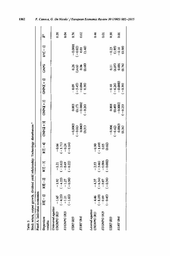
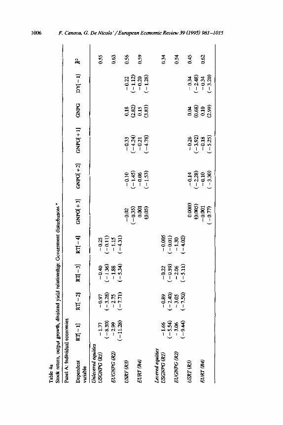
The results of our simulations appear in Tables 3-6. Tables 3 and 4 report the results of the basic simulations obtained using a symmetric specification for the model (with parameters given in the right-hand side of Table 2) and one draw for
the disturbances. Table 3 reports simulation results obtained when technology disturbances are present. Table 4 reports results when government disturbances
drive the cycle. Panels A present estimates of the regressions coefficients for domestic regressions, panels B estimates of the coefficients for international
regressions and panels C contain measures of volatility and comovements across variables.
Several features of the tables deserve attention. First, panels A show that under both specifications for the driving forces of the economy, stock returns have
predictive power for GNP growth and future GNP affects current stock returns in both countries. But in both cases, and contrary to what happens in the real data, the signs of the regressions are negative. Note also that the dividend yield is
insignificant in both stock return regressions. Second, panels B show that with both types of shocks the association of stock returns and real activity increases when international factors are included. As expected, this model specification has
a hard time to generate the asymmetries we observed in Table 1. If asymmetries are created, they are not the correct ones. Third, panels C show that the model can generate the qualitative observation that dividend yields and stock returns are more correlated than GNP across countries with both types of disturbances. However, quantitatively, the correlations are too high and, with both types of shocks, the volatility of financial variables is too low relative to the data, regardless of whether we consider unlevered or levered equities. Fourth, the dividend yield is acyclical with technology shocks and unlevered equities. With levered equities the dividend yield is too highly correlated with GNP regardless of the source of
Tab
le
3
Stoc
k re
turn
, ou
tput
gr
owth
, di
vide
nd
yiel
d re
latio
nshi
p:
Tec
hnol
ogy
dish
uban
ces
a
Pane
l A
: In
divi
dual
ec
onom
ies
Dep
ende
nt
Rfl
-l1
Rfl-
21
Rfl
--31
R
fl-4
1 G
NPG
[ +
31
GN
PG[
+ 21
G
NPG
[ +
11
GN
PG
DY
[-l]
i?
va
riab
le
Unl
ever
ed
equi
ties
USG
NP
G
(RI)
-
1.65
-
1.92
-
1.21
-0
.66
0.20
(-4.
23)
(-4.
22)
(-
2.62
) (-
1.
71)
EU
GN
PG
(R2)
-
1.21
-
1.27
-
0.49
-
0.24
0.
04
( -
1.83
) (
- 0.
58)
( -
0.22
) (-
0.14
)
USR
T
CR
.?)
-0.0
003
0.00
3 -0
.09
-0.0
001
0.76
( -
0.01
) (0
.17)
(-
5.45
) (
- 0.
02)
EU
RT
(R
4)
0.00
03
-0.0
002
- 0.
004
0.06
0.
01
0.02
(0.3
1)
( -
0.26
) (-
0.38
) (0
.68)
(1
.48)
Lev
ered
eq
uiti
es
USG
NP
G
(RI)
-
4.46
-
4.37
-
2.53
-0
.90
0.46
(-8.
19)
( -
6.34
) (-
3.66
) (-
1.
69)
EU
GN
PG
(R
2)
- 0.
89
- 0.
87
-0.0
06
0.05
0.
01
( -
0.45
) (-
0.
34)
( -
0.00
2)
(0.0
2)
USR
T
(R3)
-0
.006
0.
008
-0.1
0 0.
11
- 0.
23
0.50
( -
0.42
) (0
.49)
(-
6.26
) (6
.85)
(1
.95)
EU
RT
(R
4)
0.00
03
- 0.
0002
-
0.00
03
0.00
1 -0
.10
0.01
(0.3
6)
(-0.
25)
( -
0.39
) (0
.76)
(0
.58)

Tab
le 3
(co
nti
nu
ed)
Pan
el B
: In
tern
atio
nal
lin
kag
es
Dep
ende
nt
vari
able
U
SR
lJ -
l]
U
SR
’Ij
- 21
U
SR
’Ij
- 31
U
SR
’Ij
- 41
E
UR
fl -
l]
E
UR
’Ij -
21
EU
Rfl
-
31
EU
Rn
-
41
i?
Unl
ever
ed
equi
ties
US
GN
PG
(U
SI)
0.
33
- 1.
06
-0.1
0 -
0.01
-
3.55
-
1.63
-
1.63
-0
.66
0.30
(0.4
4)
(-
1.40
) (-
0.13
) ( -
0.
02)
(-3.
51)
(-
1.41
) (-
1.
42)
( -
0.59
)
EU
GN
PG
(E
UI)
-
2.08
-
1.70
-
1.41
-4
.15
1.43
0.
12
0.19
-0
.57
0.06
(-1.
84)
( -
0.68
) (
- 0.
59)
(-0.
18)
(0.4
3)
(0.0
3)
(0.0
5)
(-0.
15)
Leu
ered
equ
itie
s U
SGN
PG
(U
SI)
0.51
-
2.41
0.
12
0.04
-
1.98
-
2.00
-
1.52
-
0.07
0.
32
(0.7
7)
(-1.
12)
(0.9
4)
(0.5
2)
(-2.
19)
(-1.
88)
( -
1.40
) (0
.87)
EU
GN
PG
(E
UI)
-
1.99
-
1.53
1.
39
- 2.
77
C-0
.73)
(
- 0.
94)
(1.4
4)
( -
1.54
) k
:!,
0.39
0.
81
- 0.
67
0.03
(0.9
9)
(0.7
3)
(-
1.46
)
Dep
ende
nt
US
u
s u
s u
s u
s E
U
EU
E
U
EU
E
U
vari
able
G
NP
G(+
3]
GN
PG
[+2]
G
NP
G[+
l]
GN
PG
D
Y[-
I]
GN
PG
[+3]
G
NP
G[+
2]
GN
PG
[+l]
G
NP
G
Dfl
-l]
R*
Unl
ever
ed
equi
ties
USR
T (
US2
) 0.
01
(0.8
2)
EU
RT
(E
U2)
0.
006
(0.3
1)
Lev
ered
eq
uitie
s
USR
T (
lJS2
) 0.
0003
(0
.02)
EU
RT
(E
U2)
0.
0004
(0
.02)
0.01
(0.8
4)
0.01
(0
.91)
0.01
(0
.59)
0.
01
(0.5
9)
(~:~
, -0
.10
(-5.
20)
-0.1
0 0.
11
- 0.
22
0.00
01
( -
6.23
) (6
.60)
(-
1.
85)
(0.1
5)
-0.1
0 0.
11
- 0.
22
0.00
01
( -
6.23
) (6
.60)
(-
1.
85)
(0.1
5)
0.27
(15.
6)
0.13
(6.4
6)
0.11
(2
.70)
0.08
(1
.80)
- o.
ooo1
( -
0.28
)
- 0.
0002
( -
0.37
)
-0.0
01
( -
0.27
) -0
.000
1 ( -
0.2
7)
0.04
(0.1
3)
0.09
(0
.11)
0.04
(0.2
8)
0.01
(0
.28)
0.10
(1.5
2)
0.07
(0.9
7)
0.08
(1.1
9)
0.04
(1
.19)
- 0.
32
0.77
(-
2.73
) -
0.23
0.
44
(-1.
74)
- 0.
01
0.48
( -
0.03
) 0.
01
0.23
(0.1
1)

Tab
le
3 (c
ontin
ued)
.*
Pane
l C
: U
ncon
ditio
nal
mom
ents
E
B
Var
iabl
e St
anda
rd
devi
atio
ns
Cor
rela
tion
with
G
NP
Inte
rnat
iona
l co
rrel
atio
ns
.z
us
c,
Eur
ope
US
Eur
ope
,b
-1
0 1
-1
0 1
-1
0 1
2
GN
P 2.
52
1.71
0.
12
0.23
8
Con
sum
ptio
n 0.
94
-0.1
3 F
0.45
0.
06
0.16
-0
.04
0.05
0.
18
0.05
0.
02
0.06
6
Inve
stm
ent
4.13
2.
24
-0.2
2 -
0.08
0.
47
0.60
-
0.05
0.
21
0.43
0.
02
Stoc
k re
turn
s 0.
23
0.11
-
0.08
-
0.24
-
0.09
0.
82
4 -
0.03
-0
.21
0.77
-
0.01
-
0.33
0.
88
- 0.
55
4
(unl
ever
ed)
8 D
ivid
end
yiel
ds
4.46
3.
39
0.12
0.
15
0.18
-
0.03
-
0.03
-
0.02
0.
84
0.89
0.
84
(unl
ever
ed)
@
g St
ock
retu
rns
0.10
0.
11
-0.4
4 0.
51
-0.0
0 -0
.12
0.61
0.
00
- 0.
54
0.92
-0
.51
$.
(lev
ered
)
Div
iden
d yi
elds
0.
04
0.05
0.
03
0.69
-0
.07
-0.0
2 0.
02
;, 0.
09
-0.1
1 0.
94
-0.1
5 (l
ever
ed)
4.
i
a V
aria
bles
ar
e de
fine
d in
Tab
le
1; t
-sta
tistic
s ar
e in
par
enth
eses
. %
2 Y
! %

F. Canoua, G. De Nicolo’/European Economic Review 39 (1995) 981-1015 1005
disturbances. Finally, stock returns are highly positively correlated with GNP regardless of the type of disturbances driving the economy. This implies that, regardless of the type of equity employed, the effect of the two types of shocks on dividend payments is always more important than the effect on the discount factor since equity prices and returns are always positively contemporaneously associated with output fluctuations.
When we examine under which driving force the model comes closest in reproducing the data we find that the R2 of the regressions are very high when
government disturbances hit the economy while with technology disturbances the R2 are, in general, much lower. This is because, as expected, both dividend yields
and equity returns are too highly correlated with output when government shocks drive the cycle. This qualitative difference between the two types of shocks almost disappears when we consider financially levered equities because dividend yields and stock returns tend to be more procyclical when technology shocks hit the economy. This pattern persists when international regressions are considered even though the R* of the regressions with the two types of shock are more similar.
Finally, note that when the model is driven by government disturbances the domestic correlations of consumption and investment with output are too high relative to the data. In conclusion, it appears that, qualitatively, a model driven by technology disturbances is better suited to explain the data. Quantitatively, how- ever, even a model driven by technology disturbances fails to reproduce several features of the data.
Next we proceed to compare the results obtained with alternative model specifications to those of our basic setup. In particular, we are interested in
examining which source of international transmission is important in strengthening the domestic association between stock returns and real activity and whether alternative assumptions about some primitives of the model lead to different conclusions regarding the strength of the association between stock returns and real activity. To summarize the information we present a single measure of fit of
the regressions (the adjusted R2> and discuss substantial changes in other sum- mary statistics when they occur. Although this measure is clearly incomplete and may fail to capture important aspects of the data, it allows us to compactly indicate both the direction of the changes and the incremental value added by alternative features of the model.
Recall that the model displays three possible channels of international transmis- sion: first, international linkages may occur because shocks are contemporaneously correlated across countries. Second, stock returns and real activity may display international feedbacks because idiosyncratic shocks are transmitted to the world economy via production interdependencies. Third, foreign variables may carry information for domestic ones because country specific shocks are transmitted to the world economy via consumption interdependencies.
Table 5 presents the mean and the standard deviation of the adjusted R2 of international regressions for four different model specifications. The first two
Tab
le 4
a St
ock
retu
rn.
outu
ut e
row
th.
divi
dend
vie
ld r
elat
ions
hiu:
Gov
ernm
ent
dish
uban
ces
’
Pane
l A
: In
divi
dual
eco
nom
ies
Dep
ende
nt
vari
able
R
TI-
11
R7l
-21
RJI
-31
Rq-
41
GN
PGf +
31
GN
PG[ +
21
GN
PG[ +
l]
GN
PG
DY
[-11
E
2
Unl
ever
ed e
quiti
es
USG
NP
G
(RI)
-
1.77
-
0.97
-0
.40
-0.2
5 ( -
8.3
0)
(-3.
28)
(-
1.36
) (-
0.11
) E
UG
NPG
(R
2)
-2.9
9 -
2.75
-
1.88
-
1.15
(-
11.2
8)
(-7.
71)
(-5.
34)
(-4.
31)
USR
T (
R3l
) -
0.02
-0
.10
-0.3
3 0.
18
C-0
.35)
(-
1.
45)
(-
4.24
) (2
.82)
E
UR
T
(R4)
0.
001
-0.0
6 -
0.21
0.
15
(0.0
5)
(-
1.53
) (-
4.78
) (3
.83)
0.55
0.63
-0.2
2 0.
56
(-
1.12
) -0
.20
0.59
(-1.
28)
Lev
ered
eq
uitie
s
USG
NP
G
(RI)
-
1.66
-
0.89
-
0.22
-
0.00
5 0.
34
( -
5.54
) (
- 2.
40)
( -
0.59
) (-
0.01
) E
UG
NPG
(R
2)
-3.0
6 -3
.05
- 2.
06
- 1.
30
0.54
(-
9.44
) (-
7.50
) (-
5.11
) ( -
4.0
2)
USR
T t
R3)
0.
0003
-
0.14
-
0.26
0.
04
- 0.
34
0.45
(0.0
05)
(-2.
28)
(-3.
92)
(0.6
8)
(-
2.48
)
EU
RT
(R
4)
- 0.
001
-0.1
0 -0
.18
0.10
-
0.34
0.
62
( - 0
.77)
( -
3.3
0)
(-5.
25)
(2.9
9)
(-
3.20
)

Tab
le 4
(co
nti
nu
ed)
Pan
el B
: In
tern
atio
nal
lin
kag
es
Dep
ende
nt
US
R’lj
-
11
vari
able
U
SRfl
- 21
U
SR
q -
31
US
Rfl
- 41
EU
Rfl
-
l]
EU
Rl’j
-
21
EU
RT
f -
31
EU
Rd
- 41
R
2
USG
NP
G
ftiS
1,
EU
GN
PG
(E
lJl)
Un
leve
red
equi
ties
- 6.
04
- 2.
81
- 2.
69
- 1.
74
1.79
2.
56
1.92
0.
69
(-8.
19)
(-3.
55)
(-
3.46
) (
- 2.
54)
(2.2
2)
(3.2
5)
(2.5
2)
5.02
2.
48
1.23
1.
88
-8.1
9 -
4.97
-3
.14
- 3.
28
0.73
(5
.53)
(2
.54)
(1
.29)
(2
.23)
(
- 8.
53)
C-5
.01)
(-
3.23
) (-
3.51
)
Lev
ered
equ
itie
s V
SGN
PG
(U
SI)
PV
GN
PG
(133)
0.51
-2
.41
0.12
-
1.98
-2
.00
- 1.
52
- 0.
07
0.32
(0
.77)
(-
1.
12)
(0.9
4)
(-2.
19)
( -
1.88
) (-
1.
40)
(0.8
7)
- 1.
99
- 1.
53
1.39
-
2.77
0.
39
0.81
-
0.67
0.
03
(-
0.73
) (
- 0.
94)
(1.4
4)
(-
1.54
) (0
.99)
(0
873)
(-
1.
46)
.Y
Deo
ende
nt
US
u
s u
s u
s u
s E
U
EU
E
U
EU
E
U
vari
able
G
NP
G[+
31
GN
PG
[+21
G
NP
G[+
11
G
NP
G
DY
t-
11
GN
Pfl
+31
G
NP
a+2]
G
NP
G[+
l]
G
NP
G
DY
[ -
11
E2
_
Unl
ever
ed
equi
ties
U
SRT
0J
S2)
- 0.
02
0.00
1 -0
.21
0.22
-0
.42
- 0.
008
- 0.
03
-0.1
6 0.
12
0.26
0.
90
( -
0.82
) (0
.03)
(-
5.71
) (6
.98)
(
- 2.
44)
(0.4
8)
(-
1.55
) ( -
6.
98)
(5.8
5)
(1.7
1)
EV
RT
fE
U2)
-
0.01
0.
01
-0.1
9 0.
12
- 0.
25
- 0.
01
-0.0
4 -0
.17
0.15
0.
13
0.88
(
- 0.
39)
(0.4
4)
(-5.
17)
(3.8
4)
(-
1.44
) C
-0.8
1)
(-
1.87
) (-
7.
23)
(7.0
4)
(0.8
4)
Lev
ered
eq
uiti
es
USR
T
(US2
) -0
.004
-
0.03
-0
.14
0.10
-0
.15
- 0.
02
- 0.
07
-0.1
4 0.
11
- 0.
01
0.85
(-
0.15
) ( -
0.9
5)
( -
3.96
) (3
.27)
(-
1.
85)
(-
1.40
) (
- 3.
72)
(-6.
63)
(5.5
5)
( -
0.03
) E
UR
T
(EU
2)
- 0.
001
- 0.
03
-0.1
6 0.
10
-0.1
4 -
0.02
-
0.07
-0
.13
0.12
0.
01
0.86
(
- 0.
04)
(1.0
0)
( -
4.66
) (3
.14)
(-
1.
79)
(-
1.46
) (-
3.
56)
(-
6.26
) (5
.98)
(0
.23)

1008 F. Canova, G. De Nicolo’/European Economic Review 39 (1995) 981-1015
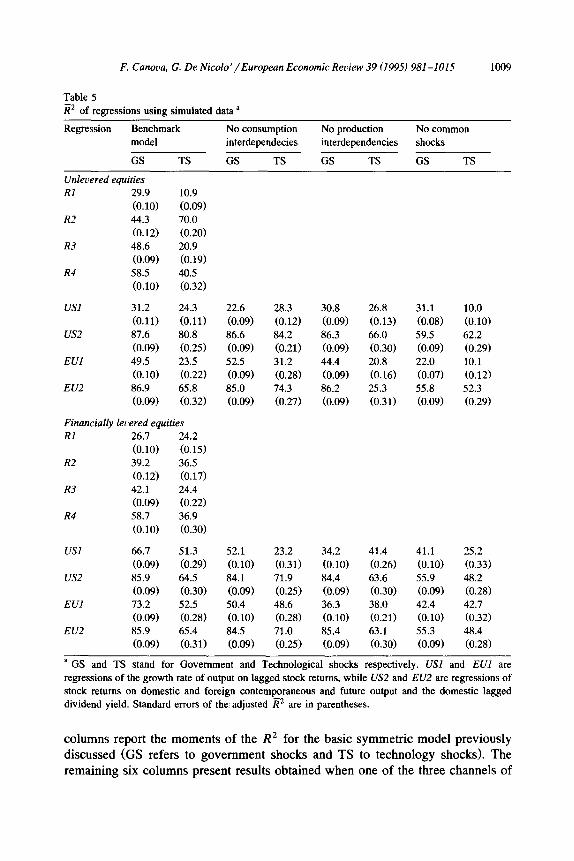
F. Canova, G. De Nicolo’/European Economic Review 39 (1995) 981-1015 1009
Table 5
i2 of regressions using simulated data a
Regression Benchmark
model
GS TS
No consumption
interdependecies
GS TS
No production No common
interdepcndencies shocks
GS TS GS TS
&levered equities
RI 29.9
(0.10)
R2 44.3
(0.12) R3 48.6
(0.09)
R4 58.5
(0.10)
10.9
(0.09)
70.0
(0.20)
20.9
(0.19)
40.5
(0.32)
US1 31.2 24.3
(0.11) (0.11)
us2 87.6 80.8
(0.09) (0.25)
EUl 49.5 23.5
(0.10) (0.22)
EU2 86.9 65.8
(0.09) (0.32)
22.6
(0.09)
86.6
(0.09) 52.5
(0.09) 85.0
(0.09)
28.3
(0.12)
84.2
(0.21)
31.2
(0.28)
74.3
(0.27)
30.8
(0.09) 86.3
(0.09)
44.4
(0.09)
86.2
(0.09)
26.8
(0.13)
66.0
(0.30) 20.8
(0.16) 25.3
(0.31)
31.1
(0.08)
59.5
(0.09)
22.0
(0.07)
55.8
(0.09)
10.0
(0.10)
62.2
(0.29)
10.1
(0.12)
52.3
(0.29)
Financially levered equities
RI 26.7 24.2
(0.10) (0.15)
R2 39.2 36.5
(0.12) (0.17) R3 42.1 24.4
(0.09) (0.22)
R4 58.7 36.9
(0.10) (0.30)
us1 66.7 51.3 52.1 23.2 34.2 41.4 41.1 25.2
(0.09) (0.29) (0.10) (0.31) (0.10) (0.26) (0.10) (0.33)
us2 85.9 64.5 84.1 71.9 84.4 63.6 55.9 48.2
(0.09) (0.30) (0.09) (0.25) (0.09) (0.30) (0.09) (0.28)
EUl 73.2 52.5 50.4 48.6 36.3 38.0 42.4 42.7
(0.09) (0.28) (0.10) (0.28) (0.10) (0.21) (0.10) (0.32)
EU2 85.9 65.4 84.5 71.0 85.4 63.1 55.3 48.4
(0.09) (0.31) (0.09) (0.25) (0.09) (0.30) (0.09) (0.28)
a GS and TS stand for Government and Technological shocks respectively. US1 and EVl are
regressions of the growth rate of output on lagged stock returns, while US2 and EV2 are regressions of
stock returns on domestic and foreign contemporaneous and future output and the domestic lagged
dividend yield. Standard errors of the adjusted E2 are in parentheses.
columns report the moments of the R2 for the basic symmetric model previously discussed (GS refers to government shocks and TS to technology shocks). The remaining six columns present results obtained when one of the three channels of

1010 F. Canova, G. De Nicolo ‘/ European Economic Review 39 (I 995) 9814015
international transmission is sequentially closed. In the third and fourth columns we eliminate consumption interdependencies (setting 8,j = 0 for h #i, h, i = 1, 2, 31, in the fifth and sixth columns we eliminate production interdependencies (setting czhj = 0 for h #i, h, j = 1, 2, 31, and in the last two columns we eliminate contemporaneous correlations across shocks (by requiring Z1 or Z2 to be diagonal). The mean and the standard deviations of the adjusted R* are obtained by drawing 1000 time series for each type of shock, constructing 1000 time series for the endogenous variables of the model using calibrated parameters and running 1000 times the regressions of interest.
When government expenditure shocks drive the economy, the three sources of transmission are equally important, regardless of the definition of equity consid- ered. However, the drop in the R* of the international regressions is larger when contemporaneous correlations are eliminated. When technology disturbances drive the cycle, we see that the elimination of each of the three sources of international interdependencies actually increases the adjusted R* of the regressions, indicating that, within the current parameterization of the model, the three effects do not all go in the same direction. In conclusion, the results suggest that international data help in strengthening the relationship between domestic stock returns and domestic GNP growth because they provide information about the likely magnitude of the feedbacks across countries. Overall all three channels of international transmission are important to explain the international linkages between stock returns and real activity we see in the data. Relatively speaking, the effect of production interde- pendencies is larger when technology shocks drive the international cycle, while the effect of consumption interdependencies is more important when government shocks drive the cycle.
The current parameterization of the model is incapable of reproducing the asymmetric international feedbacks we presented in Table 1. In principle, asymme- tries would have emerged if there were important differences in preferences, production possibilities, or per-capita wealth across countries. The current specifi- cation does allow for asymmetries in production possibilities (the share of domestic capital in production is larger than the share of foreign capital) but it makes preferences, installation costs and per-capita wealth perfectly symmetric across countries. However, the home-bias we have introduced in production does not seem to be to crucial to generate those asymmetries we care about.
For this reason, we next examine whether the introduction of these features alters the properties of our reduced form regressions. To do this we proceed in three steps. First, we would like to measure the effect of introducing asymmetric installation costs in the model, where by asymmetric we mean that the cost of installing foreign capital is larger than the cost of installing domestic capital. In principle, this should increase the strength of the association between domestic stock returns and domestic real activity when technology disturbances drive the cycle but have negligible effects when government shocks drive the cycle and decrease the association between domestic and foreign real variables. Second, we
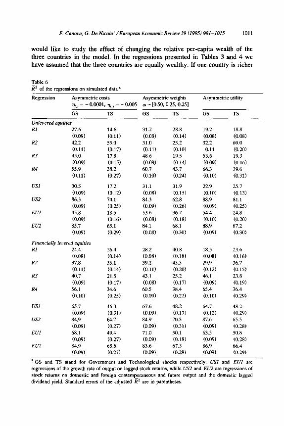
F. Canova, G. De Nicolo’/European Economic Review 39 (1995) 981-1015 1011
would like to study the effect of changing the relative per-capita wealth of the three countries in the model. In the regressions presented in Tables 3 and 4 we have assumed that the three countries are equally wealthy. If one country is richer
Table 6
R* of the regressions on simulated data a
Regression Asymmetric costs Asymmetric weights Asymmetric utility
rki = -0.0001, r$ , = - 0.005 o = [0.50, 0.25,0.25]
GS TS GS TS GS TS
Unlevered equities
RI 27.6
(0.09)
R2 42.2 (0.11)
R3 45.0
(0.09)
R4 55.9
(0.11)
US1 30.5
(0.09)
us2 86.3
(0.09)
EUl 45.8
(0.09) EU2 85.7
(0.09)
Financially levered equities
RI 24.4
(0.08)
R2 37.8
(0.11)
R3 40.7
(0.09)
R4 56.1
(0.10)
us1 65.7
(0.09)
us2 84.9 (0.09)
EUl 68.1
(0.09) EU2 84.9
(0.09)
14.6
(0.11)
55.0
(0.17)
17.8
(0.15)
38.2
(0.27)
17.2
(0.12)
74.1
(0.25)
18.5
(0.16)
65.1
(0.29)
26.4
(0.14)
35.1
(0.14)
21.5
(0.17)
34.6
(0.25)
46.3
(0.31)
64.7
(0.27)
49.4
(0.27)
65.6 (0.27)
31.2
(0.08)
31.0
(0.11)
48.6
(0.09) 60.7
(0.10)
31.1
(0.08)
84.3
(0.09) 53.6
(0.08)
84.1
(0.08)
28.2
(0.08)
39.2
(0.11)
43.1
(0.08)
60.5
(0.09)
67.6
(0.09) 84.9
(0.09) 71.0
(0.09)
83.6
(0.09)
28.8 19.2
(0.14) (0.08)
25.2 32.2
(0.10) 0.11
19.5 53.6
(0.14) (0.09)
43.7 66.3
(0.24) (0.10)
31.9
(0.15)
62.8
(0.26)
36.2
(0.18)
68.1
(0.30)
22.9
(0.10)
88.9
(0.09)
54.4
(0.10)
88.9
(0.09)
40.8
(0.18)
45.5
(0.20)
25.2
(0.17)
38.4
(0.22)
18.3
(0.08)
29.9
(0.12)
46.1
(0.09)
65.4
(0.10)
48.2
(0.17)
70.3
(0.31)
50.1
(0.18)
67.3 (0.29)
64.7
(0.12)
87.6
(0.09)
63.3
(0.09)
86.9 (0.09)
18.8
(0.08)
69.0
(0.20)
19.3
(0.16)
39.6
(0.31)
25.7
(0.13)
81.1
(0.25)
24.8
(0.20)
67.2
(0.30)
23.6
(0.16)
36.7
(0.15)
23.8
(0.19)
36.4
(0.29)
48.2
(0.29)
65.5
(0.28)
50.8
(0.28)
66.4
(0.29)
a GS and TS stand for Government and Technological shocks respectively. US1 and EUl are
regressions of the growth rate of output on lagged stock returns, while US2 and EU2 are regressions of
stock returns on domestic and foreign contemporaneous and future output and the domestic lagged
dividend yield. Standard errors of the adjusted R2 are in parentheses.

1012 F. Canova, G. De Nicolo’/European Economic Review 39 (1995) 981-1015
(or larger) than th e others, we should expect more asymmetries in international linkages and a better match with the actual data with both types of shocks. Third, we would like to examine the effect of introducing asymmetries in preferences across countries. In this case we assume that agents prefer to consume a larger share of their own produced good (cx,,~ = 0.30, (Y,,~ = 0.02, h # j> which is more in line with estimates of the share parameters presented in Table 2. Note that with asymmetries in utility, we price assets using the discount factor of the fictitious representative agent. This implies that the volatility of the discount factor we use may be higher and the effect of various disturbances on the discount factor may be larger relative to the one on dividend payments. It is therefore of interest to know, in particular when government shocks drive the cycle, if this feature is sufficient to produce countercyclical dividends and reduce the adjusted R2 of the regressions to the range of values observed in the data.
Table 6 presents the mean and the standard deviation of the adjusted R2 for regressions conducted with these alterations of the basic model. As before, GS indicates the case of a model driven by government disturbances and TS the case of a model driven by technology shocks. The results suggest that, although the changes induce the desired effect, the quantitative magnitude of the impact is small. Three features of the table are worth mentioning. First, with financially levered equities the effect of introducing asymmetric installation costs is negligible for both types of shocks. Second, changing the social planner weights has some effect in international regressions only when technology disturbances drive the cycle and primarily for the ‘small’ country (which, in our case is Europe). Third, the introduction of asymmetries in the utility function produces no changes when technology disturbances driving the cycle while with government disturbances the magnitude of the changes is small.
In conclusion, even with the three above modifications the model fails to generate the asymmetries in international regressions. To produce such a pattern it seems necessary to work with a model displaying a much more complicated asymmetric transmission mechanism of shocks.
7. Conclusions
In this paper we have examined the relationship between stock returns and real activity from the point of view of an international general equilibrium model where agents are rational and markets are complete. We focused on three questions: first, what kind of shocks are likely to move asset returns and real activity. Second, which channels of domestic transmission are crucial to link financial markets and real activity. Third, what type of international linkages are necessary to generate the relationship between asset returns and real activity we see in international data.
We show that the model can produce the type of association between domestic stock returns and domestic real activity we see in the data but, with unlevered
F. Canova, G. De Nicolo’ / European Economic Review 39 (1995) 981-l 015 1013
equities, the strength of the association depends on the source of disturbances driving the cycle. With financially levered equities this qualitative distinction fades. We find that when government expenditure shocks drive the international cycle the association between real GNP growth and stock returns is primarily due to the strong positive effect these disturbances have on dividend payments. When
technology shocks drive the cycle, the association is weaker because dividend yields are less correlated with GNP. We also demonstrated that our model produces some important cross country spillovers between stock returns and real activity and that all three possible channels of international transmission that the
model displays are crucial in generating the type of cross country linkages we see in the actual data. Finally, we show that the introduction of asymmetries in the
model does not quantitatively help to match the asymmetries we see in the data even though, qualitatively, the changes occurring are in the right direction.
Acknowledgment
We would like to thank three anonymous referees, Albert0 Giovannini, Bob
Hodrick, Anil Kashyap and Harald Uhlig for providing detailed and useful comments on earlier versions of the paper and Bernard Dumas, Mervin King, Pat Kehoe, Bill Branson and the participants of the Conference ‘International Stock
Returns and the Business Cycle’, London, UK and the 17th ‘ISOM Conference’, Paris, France and of seminars at Universitat Pompeu Fabra, Brandeis University
and Institute for Economic Analysis for suggestions.
References
Aiyagari, R., L. Christian0 and M. Eichenbaum, 1992, The output, employment and interest rate effects
of government consumption, Journal of Monetary Economics 30, 73-86.
Backus, D., P. Kehoe and F. Kydland, 1992, International business cycles, Journal of Political
Economy 100, 735-775.
Backus, D., P. Kehoe and F. Kydland, 1993, Dynamics of trade balance and the terms of trade: Is there
a J-curve?, American Economic Review 84, 84-103.
Balvers, J., T. Cosimano and B. McDonald, 1990, Predicting stock returns in an efficient market,
Journal of Finance XLV, 1109-1135.
Baxter, M. and M. Crucini, 1991, Business cycle and the asset structure of foreign trade, Manuscript
(University of Rochester, Rochester, NY).
Baxter, M. and M. Crucini, 1993, Savings and investment correlations, American Economic Review
83, 416-436.
Bekaert, G. and R. Hodrick, 1992, Characterizing predictable components in excess returns on equity
and foreign exchange markets, Journal of Finance XLVII, 467-509.
Brown, D. and M. Gibbons, 1985, A simple econometric approach for utility based asset pricing
models, Journal of Finance XL, 359-381.

1014 F. Canova, G. De Nicolo’/European Economic Review 39 (1995) 981-1015
Bums, A. and W. Mitchell, 1943, Measuring business cycles (NBER Press, Cambridge, MA).
Campbell, J. and ? Ammer, 1993, What moves the stock and bond markets? A variance decomposition
for long-term asset returns, Journal of Finance XLVIII, 3-37.
Canova, F., 1993, Sources and transmission of international business cycles, Working paper 781
(CEPR, London).
Canova, F. and G. De Nicolo’, 1995, The equity premium and the risk free rate: A cross country, cross
maturity investigation, Working paper 1015 (CEPR, London).
Canova, F. and J. Mar&an, 1995, Predicting excess returns in financial markets, European Economic
Review 39, 35-69.
Cardia, E. 1991, The dynamics of a small open economy in response to monetary, fiscal and
productivity shocks, Journal of Monetary Economics 28, 411-434.
Christiano, L. and M. Eichenbaum, 1992, Current real business cycle theories and aggregate labor
market fluctuations, American Economic Review 82, 430-450.
Constantinides, G. and D. Duffie, 1992, Asset prices with heterogeneous consumers, Manuscript
(University of Chicago, Chicago, IL).
Costello, D., 1991, Trade in intermediate goods and international business cycles, Manuscript.
(University of Florida, Gainesville, FL).
Cutler, D., J. Poterba and L. Summers, 1989, What moves stock prices, Journal of Portfolio
Management 15, 4-12.
Danthine, J.P. and J. Donaldson, 1986, Inflation and asset prices in an exchange economy, Economet-
rica 54, 585-605.
Danthine, J.P. and J. Donaldson, 1994, Asset pricing implications of real market frictions, Manuscript
(Columbia University, New York).
Fama, E., 1990, Stock returns, expected returns and real activity, Journal of Finance XLV, 1089-1108.
Fama, E. and K. French, 1988, Dividend yields and expected stock returns, Journal of Financial
Economics 22, 3-25.
Finn, M., 1991, Energy price shocks, capacity utilization and business cycle fluctuations, empirical
institute, Discussion paper 50 (Federal Reserve Bank of Minneapolis, Minneapolis, MN).
Harris, T. and T. Opler, 1990, Stock market returns and real activity: International evidence,
Manuscript (UCLA, Los Angeles, CA).
King, R., C. Plosser and S. Rebelo, 1988, Production, growth and business cycles I: The basic
neoclassical model, Journal of Monetary Economics 21, 195-232.
Jeager, A., 1991, The slope of the yield curve as predictor of business cycle fluctuations, Working
paper 46 (WIFO, Vienna).
Jermann, U., 1994, Asset pricing in production economies, Manuscript (Wharton School, Philadelphia,
PA).
Masulis, R., 1988, Debt-equity choice (Ballinger, Cambridge, MA).
Mendoza, E., 1991, Real business cycles in a small open economy, American Economic Review 81,
797-818.
Plosser, C. and G. Rowenhorst, 1994, International term structures and real economic growth, Journal
of Monetary Economics 33, 133-155.
Prescott, E. and R. Mehra, 1980, Recursive competitive equilibrium: The case of homogeneous
households, Econometrica 48, 1365-1379.
Reynolds, P., 1993, International comovements in production and consumption: Theory and evidence,
Manuscript (USC, Los Angeles, CA). Roll, R., 1988, R*, Journal of Finance 43, 541-566.
Rowenhorst, G., 1991, Asset returns and the business cycle, Unpublished Ph.D. Dissertation (Univer-
sity of Rochester, Rochester, NY).
Rotemberg, J. and M. Woodford, 1992, Oligopolistic pricing and the effect of aggregate demand on
economic activity, Journal of Political Economy 100, 1153-1207.

F. Canoua, G. De Nicolo’ / European Economic Review 39 (1995) 981-1015 1015
Schwert, W., 1990, Stock returns and real activity: A century of evidence, Journal of Finance XLV,
1237-1257.
Stock, J. and M. Watson, 1989, A new index of coincident and leading indicators, NBER Macroeco-
nomic Annual, 351-394.
Stockman, A. and L. Tesar, 1994, Tastes and technology in a two country model of the business cycles:
Explaining international comovements, American Economic Review, forthcoming.