stock market trend prediction using markov models

©ELECTRON Department of ECE, Amrita Vishwa Vidyapeetham, Coimbatore

Conference Proceedings RTCSP’09 285

Stock market trend prediction Using markov models

Prof. R. Sundararajan, Aswath Kumar P N, Badri Krishnan K N, Dinesh R, Karthikeyan S, Sridhar C

Department of Electronics and Communication Amrita School of Engineering, Coimbatore

[email protected], [email protected], [email protected]

Abstract: A Markov Chain is a special kind of Stochastic Process which is largely used to study the probability of the evolution of a system over a period of time. It is being extensively used in the field of physics, bio-informatics, mathematical theory of communication etc, rarely used in the field of stock market analysis. By using the first order Markov chain model, the returns are classified into bull and bear states and their transition between these two states are recorded by constructing a transition probability matrix, and their speed of convergence to the steady state is used as measure of market efficiency. The present study aims at predicting the stock market trend using a Stochastic Markov Chain Model. This model can be related to feed forward control loop where the error is already predicted before it affects the output. In addition to markov chain, prediction is also done using Hidden Markov Model and the results are compared. The data of various volume is taken as input and its influence on the prediction is analysed.

1. Introduction

A large number of research works are carried out to study the share price behavior and efficiency of Market. It must be admitted that every study provided new insights on the share price behavior. It can be seen that most of the studies on stock market predictability have used traditional statistical techniques. But there are exceptions Kaushik Bhattacharya (2002) specified a two state Markov Chain Model on the categorized returns and proposed a measure for financial market efficiency. The

model specified gives a new method for measuring market efficiency by borrowing concepts from the literature of mobility indices. There are various methods used in stock market Prediction such as Hidden Markov Model, Neural Networks, Rough Set Theory, Artificial Intelligence, Random Walk Hypothesis and Genetic Algorithm. Markov Model is basically the generation of any sequence. There are many states involved with any sequence. The value of the system switches between any of these states. The probability of the value to occupy a state depends on the previous states. The hidden Markov model (HMM) is a probabilistic method used to determine the behavior of a time varying system. Since this is a probabilistic method, more the data we consider for applying in the Markov model, more accurate are the results. The basic approaches employed in the Hidden Markov Model will be discussed in this paper.

2. Testing for dependency

This is necessary to check the data that is being given as input is dependent or not, since the independent/random data cannot be predicted using this model. Efficient Market Hypothesis, which is the underlying principle behind this, states that “All stock prices are independent provided the autocorrelation results of the series are within the acceptable range (95% confidence level), has been used here. Autocorrelation function which defines the relationship between the present value and the previous values of a time series data is used to check the dependency of the stock

Administrator

Highlight

Administrator

Highlight



price returns. Autocorrelation is done using a function available in MATLAB

autocorr(Series,Lags,M,nSTDs)

Series - vector of time series observations for which autocorrelation has to be performed.

Lags - positive scalar integer indicating the number of past data which has to be correlated with present data. Lags=min([230,length(series)-1])

M - Nonnegative integer scalar indicating the number of lags beyond which the theoretical ACF is effectively 0. M must be less than nLags.

nSTDs – confidence limit. The default is value is 2 (i.e. approximately 95% confidence interval).

3. Markov chain

To apply Markov process to share market behavior, share price can be view a system toggling between bullish and bearish state. The share price returns at time n is given as,

R= (sp (n)-sp (n-1))/sp (n-1),

Where

1) sp(n) is today’s closing price 2) sp(n-1) is yesterday’s closing price

We define a set of random variables.

Bull, R> 0,

Bear, R<0

Assuming that R follows a stationary first order Markov chain and future movement of R depends only on its current state. A 2X2 Transition probability matrix of R gives the probability of all possible transitions between all possible states. We construct the matrix from the past behavior of the system and the

transition probability matrix in conjunction with the probability values of the present.

States/States Bull Bear

Bull P11 P12

Bear P21 P22

Table1. Transition Probability Matrix (P)

Pij is the probability of moving from state i to state j.

0< Pij< 1 and Pil + Pi2 = 1 for i = 1, 2;

j = 1, 2

By considering the closing price of last and last before observations we fix the state probability vector

π = [1 0] for bullish and

π = [0 1] for bearish.

Using this notation, the steady state probabilities for period n+1 is obtained by multiplying the known state probabilities for period n by the transition probability matrix. Using the vector of state probabilities and the matrix of transition probabilities, the multiplication can be expressed.

The representation is,

π (future) = π (current) * P

(or)

π. (n+1) = π (n) * P

The state probabilities TI1 (1) = 0.49 and TI2 (1) = 0.51 are the probabilities that a bearish trend previous day will follow a bullish trend during the 1st day. Similarly using the same equation the state probabilities for the second day, third day can be computed as follows:

Administrator

Highlight



π (2) = π(1) * P

π (3) = π(2) * P

As we continue the Markov process, it can be seen that the probability of the system attains steady state within few days, implies the market is efficient/stable. The probability that is obtained after few transitions is referred to as the steady-state probabilities.

4. Hidden Markov Model (HMM)

The model requires two important parameters namely, Transition probability matrix and Emission/observation matrix. Transition probability matrix is same as that calculated in markov chain. A 2X4 emission matrix whose i,j entry gives the probability of emitting symbol sj given that the model is in state i.

States/Symbols p-p p-n n-p n-n

Bull P11 P12 P13 P14Bear P21 P22 P23 P24

Table2. Emission Matrix

The future sequence and the states to which it might jump are generated using function available in MATLAB.

[seq ,states]= hmmgenerate(len,trans,emis)

• trans - transition probability matrix • emis - emission probability matrix • len - length of both seq and states • seq – sequence of emission symbol • state - sequence of states

4.1 Advantages of HMM

• In this method accuracy is higher when compared to other methods (~65%).

• It has strong statistical foundation

• It is able to handle new data robustly

• Computationally efficient to develop and evaluate due to existence of established training algorithms.

5. Experimental Results

Stock data for about 1 year (Jan.1 2007 to Dec.15 2007) are taken for analysis and the working of the model is verified for the next 10 days. The closing price for each company is considered and the returns are calculated.

5.1 Tests for Dependency

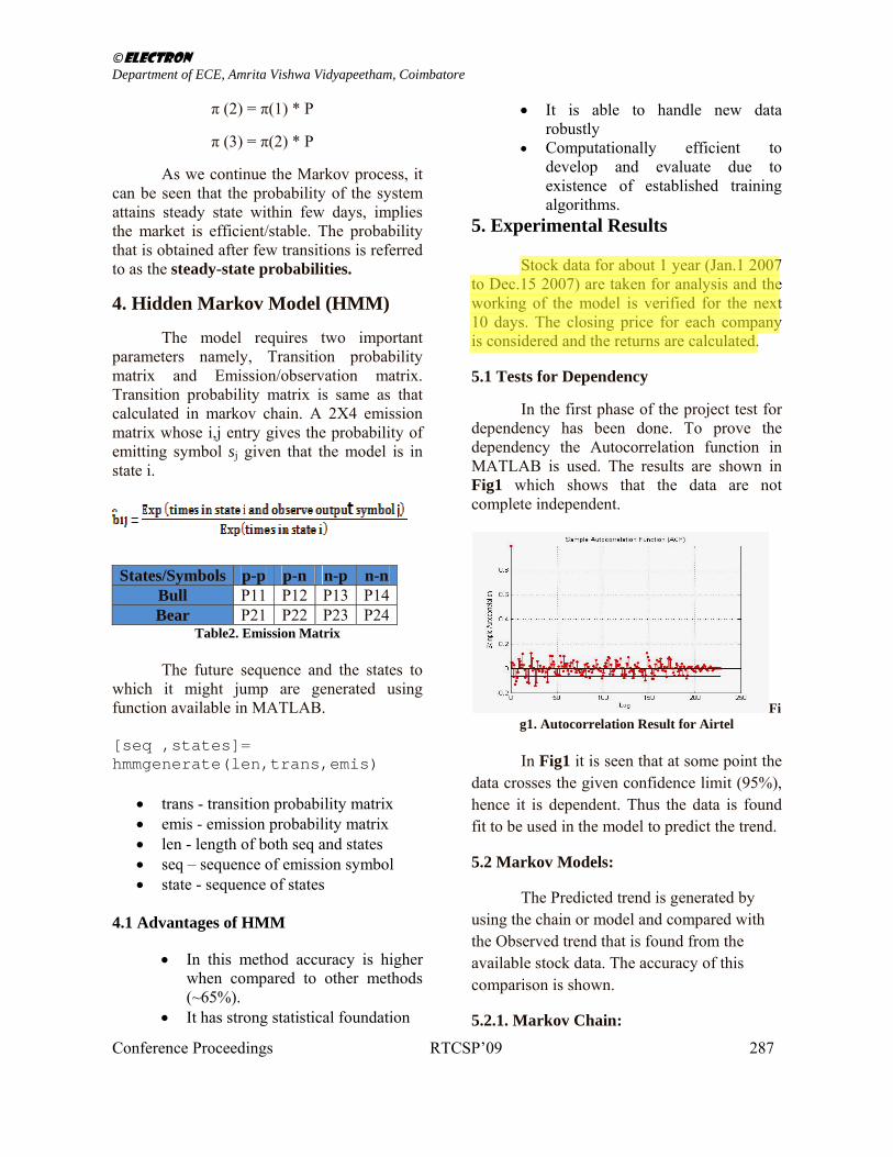
In the first phase of the project test for dependency has been done. To prove the dependency the Autocorrelation function in MATLAB is used. The results are shown in Fig1 which shows that the data are not complete independent.

Fig1. Autocorrelation Result for Airtel

In Fig1 it is seen that at some point the data crosses the given confidence limit (95%), hence it is dependent. Thus the data is found fit to be used in the model to predict the trend.

5.2 Markov Models:

The Predicted trend is generated by using the chain or model and compared with the Observed trend that is found from the available stock data. The accuracy of this comparison is shown.

5.2.1. Markov Chain:

Administrator

Highlight



The results of the Markov chain are shown in Table3. In general the trend prediction stabilizes in around 4 to 7 days.

Day Predicted Trend

Observed Trend

1 Bear Bull 2 Bull Bull 3 Bull Bear 4 Bull Bull 5 Bull Bull 6 ‐ Bull 7 ‐ Bear 8 ‐ Bear 9 ‐ Bull 10 ‐ Bear

Accuracy = 60% Table 3: Markov Chain Result

From Table3, for Airtel we found that the prediction converges in 5 days, which means the market is stable.

5.2.2. Markov Model:

The results of the Markov chain are shown in Table4.

Table 4: Markov Model Result

The trend for next 10 days is predicted for the same company Airtel, the accuracy matches with that of the markov chain method of prediction.

5.3 Value Prediction Results:

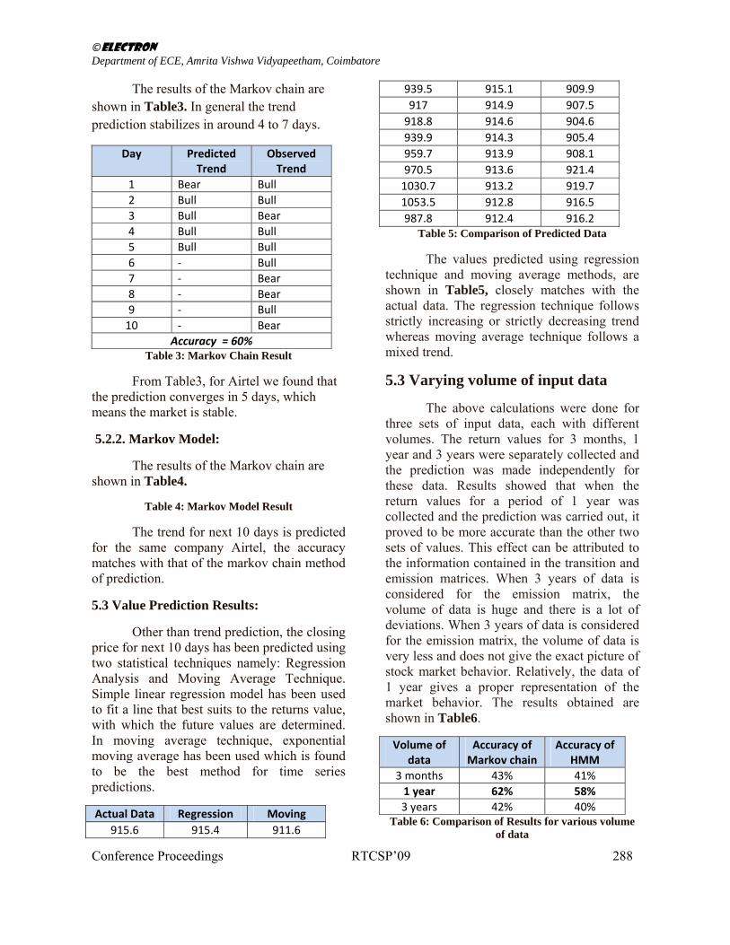
Other than trend prediction, the closing price for next 10 days has been predicted using two statistical techniques namely: Regression Analysis and Moving Average Technique. Simple linear regression model has been used to fit a line that best suits to the returns value, with which the future values are determined. In moving average technique, exponential moving average has been used which is found to be the best method for time series predictions.

Actual Data Regression Moving 915.6 915.4 911.6

939.5 915.1 909.9917 914.9 907.5 918.8 914.6 904.6 939.9 914.3 905.4 959.7 913.9 908.1970.5 913.6 921.41030.7 913.2 919.7 1053.5 912.8 916.5 987.8 912.4 916.2

Table 5: Comparison of Predicted Data

The values predicted using regression technique and moving average methods, are shown in Table5, closely matches with the actual data. The regression technique follows strictly increasing or strictly decreasing trend whereas moving average technique follows a mixed trend.

5.3 Varying volume of input data

The above calculations were done for three sets of input data, each with different volumes. The return values for 3 months, 1 year and 3 years were separately collected and the prediction was made independently for these data. Results showed that when the return values for a period of 1 year was collected and the prediction was carried out, it proved to be more accurate than the other two sets of values. This effect can be attributed to the information contained in the transition and emission matrices. When 3 years of data is considered for the emission matrix, the volume of data is huge and there is a lot of deviations. When 3 years of data is considered for the emission matrix, the volume of data is very less and does not give the exact picture of stock market behavior. Relatively, the data of 1 year gives a proper representation of the market behavior. The results obtained are shown in Table6.

Volume of data

Accuracy of Markov chain

Accuracy of HMM

3 months 43% 41%1 year 62% 58% 3 years 42% 40%

Table 6: Comparison of Results for various volume of data



6. Conclusion

The primary focus of the study is to predict the stock market trend and measure the stock market efficiency by applying the First Order Markov Chain Model. When the Markov Chain Model is applied to predict the trend of the stock prices, the result of the tests and comparison with other competitive methods show that the model could predict the trend only for a few days and the system attains a steady state within a few trials in case of majority of the shares implying that the stock market trend could not be predicted very accurately, which means that the market is stable.

7. References

[1] Study on Stock Market Trend Prediction and Market Efficiency Using First Order Markov Chain Model – M.V. Subha and S. Thirupparkadal Nambi. Second national conference on Management Science and Practice, March 9-11, 2007 in IIT-Madras.

[2] Introduction to Hidden Markov Model and Its Application, Dr. Sung-Jung Cho, Samsung Advanced Institute of Technology (SAIT), April 16, 2005.

[3] An Introduction to Hidden Markov Models, L. R.Rabiner and B. H. Juang, IEEE ASSP MAGAZINE JANUARY 1986.

[4] Financial Management theory and Practice, Prasanna Chandra, chapter 6, Second edition, TATA McGraw Hill, 1984.

[5] Fundamentals of STOCK MARKET by B. O'Neill Wyss, McGraw Hill, copyright 2001, chapters 1-5.

[6] Rough Sets by Lin Shang, Department of Computer Science and Technology, Nanjing University.

stock market trend prediction using markov models

Documents