Arnold Sommerfeld Center for Theoretical Physics Prof. Dr. E. FreyLudwig-Maximilians-Universitat Munchen M. Weber, C. Weig

Stochastic Processes in Physics and Biology – Exercise sheet 6Winter term 2011/2012

Exercise 13 Fluctuation Driven Ratchets

Download the paper: R.D.Astumian and M.Bier, “Fluctuation Driven Ratchets: Molecular Motors”, Phys. Rev.Lett., 1994, 72 (11), 1766–1769 from http://prl.aps.org/abstract/PRL/v72/i11/p1766 1.

a) Reading:

• Read the abstract and the introduction of the paper up to the end of the first page. Try to get an ideaabout the kind of models studied in the paper.

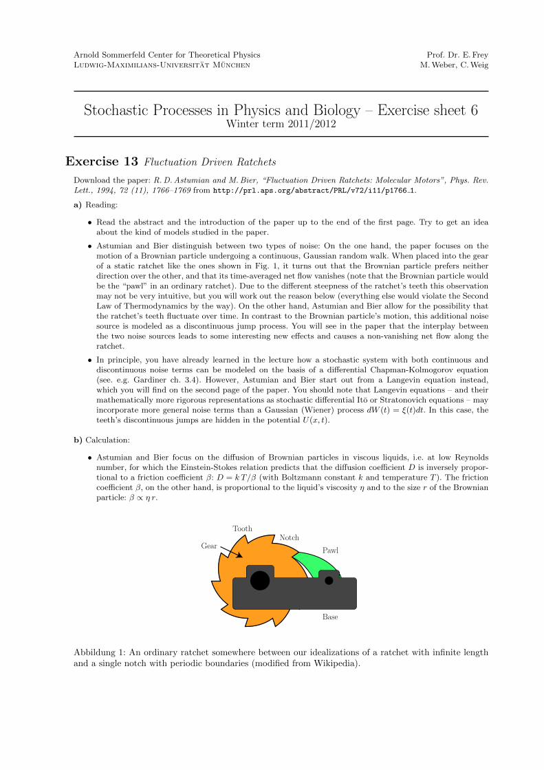
• Astumian and Bier distinguish between two types of noise: On the one hand, the paper focuses on themotion of a Brownian particle undergoing a continuous, Gaussian random walk. When placed into the gearof a static ratchet like the ones shown in Fig. 1, it turns out that the Brownian particle prefers neitherdirection over the other, and that its time-averaged net flow vanishes (note that the Brownian particle wouldbe the “pawl” in an ordinary ratchet). Due to the different steepness of the ratchet’s teeth this observationmay not be very intuitive, but you will work out the reason below (everything else would violate the SecondLaw of Thermodynamics by the way). On the other hand, Astumian and Bier allow for the possibility thatthe ratchet’s teeth fluctuate over time. In contrast to the Brownian particle’s motion, this additional noisesource is modeled as a discontinuous jump process. You will see in the paper that the interplay betweenthe two noise sources leads to some interesting new effects and causes a non-vanishing net flow along theratchet.

• In principle, you have already learned in the lecture how a stochastic system with both continuous anddiscontinuous noise terms can be modeled on the basis of a differential Chapman-Kolmogorov equation(see. e.g. Gardiner ch. 3.4). However, Astumian and Bier start out from a Langevin equation instead,which you will find on the second page of the paper. You should note that Langevin equations – and theirmathematically more rigorous representations as stochastic differential Ito or Stratonovich equations – mayincorporate more general noise terms than a Gaussian (Wiener) process dW (t) = ξ(t)dt. In this case, theteeth’s discontinuous jumps are hidden in the potential U(x, t).

b) Calculation:

• Astumian and Bier focus on the diffusion of Brownian particles in viscous liquids, i.e. at low Reynoldsnumber, for which the Einstein-Stokes relation predicts that the diffusion coefficient D is inversely propor-tional to a friction coefficient β: D = k T/β (with Boltzmann constant k and temperature T ). The frictioncoefficient β, on the other hand, is proportional to the liquid’s viscosity η and to the size r of the Brownianparticle: β ∝ η r.

Gear Pawl

Base

ToothNotch

Abbildung 1: An ordinary ratchet somewhere between our idealizations of a ratchet with infinite lengthand a single notch with periodic boundaries (modified from Wikipedia).

Consider the Langevin equation

˙x(t) = − ∂

∂xU(x, t) + ζ(t) ,

〈ζ(t)〉 = 0 ,

〈ζ(t) ζ(t′)〉 = 2Dδ(t− t′) ,

and rescale time by the diffusion constant, t = D t, to obtain the Langevin equation used by Astumian andBier with correlation function: 〈ξ(t) ξ(t′)〉 = 2δ(t− t′).

• Proceed to the models discussed under (i) and (ii) on the second page of the paper. Write down the equationsfor the potential U(x, t) for both cases and check your equations against the ratchets shown in Fig. 1. Notethat there are some minor sign errors in part (i). You should interpret the fluctuating terms ∆F (t) and∆E(t) as trajectories of a telegraph process, and compare the model with the switching genetic operatorsdiscussed by Kepler and Elston (see exercise sheets 2 and 3).

• (Bonus) Combine the Gillespie and Langevin algorithms from the previous exercises to generate sampletrajectories of the Langevin equation. Use the Gillespie algorithm to find the times at which the telegraphprocess switches between different states of the ratchet. You may then use an explicit Euler algorithm tointegrate over the Gaussian noise of the Ito SDE that corresponds to the Langevin equation. Note that yourtime step should be sufficiently small such that the particle cannot jump from one notch into another in asingle integration step (roughly ∆t = 0.00001 for the parameters used in the paper; you should, however,tune the amplitudes of the fluctuations to ∆F , ∆E ≈ 7 to get nice trajectories, as shown on the next side).

• Assume for a moment that the potential U(x, t) does not fluctuate over time, and that the Gaussian noiseterm η(t) is the only source of stochasticity. Derive a Fokker-Planck equation for the conditional probabilitydensity function P (x, t|x0, t0) of finding the particle around position x ∈ R. In principle, you could do so bymapping the Langevin equation to an Ito SDE first. But since most physics papers are written in terms ofLangevin equations, you should not do so. It is an important skill to deal with historical or sloppy notation(the noise term of Langevin equations is plagued by an infinite variance in contrast to SDEs). You maystart out from the Langevin equation’s integral representation

x(t+ ∆t) = x(t) +(− ∂

∂xU(x, t)

)∆t+

∫ t+∆t

t

ds ζ(s) ,

and derive the Fokker-Planck equation by considering the mean of a non-anticipatory test function f(x(t)),just as we did on the last exercise sheet.

• Since you probably did not encounter so many Fokker-Planck equations before (although quite a fewSchrodinger equations), let us consider a simple problem first. As warm-up, assume that the particle isdriven by a constant force F (x, t) = F :

∂tP (x, t|x0, t0) = −F∂xP (x, t|x0, t0) + ∂2xP (x, t|x0, t0) with P (x, t0|x0, t0) = δ(x− x0) .

Use the Fourier transformation

φ(k, t|x0, t0) =

∫Rdx eikxP (x, t|x0, t0)

to show that the Fokker-Planck equation is solved by a Gaussian with mean µ = x0 + F (t− t0) and varianceσ2 = 2(t− t0). Does the Fokker-Planck equation admit a stationary solution?

• Astumian and Bier’s model does not admit such a solution. In order to show that the ratchet’s fluctuatingteeth may cause a non-vanishing particle flow along the ratchet, they focus on a single notch and assu-me periodic boundary conditions. If this reduced model admits a stationary solution with non-vanishingprobability flow, such a flow may also assumed for the infinitely long ratchet (since particles crossing theboundary in the flow’s direction get trapped in the next notch). As a first step, show that a static ratcheton the interval x ∈ [0, 1] with periodic boundaries does not admit such a probability flow. For this purpose,rewrite the Fokker-Planck equation as a continuity equation by introducing the probability flux/flow J :

∂tP (x, t|·) + ∂xJ(x, t|·) = 0 ,

with J(x, t|·) = F (x)P (x, t|·)− ∂xP (x, t|·) .

By noting that the force F (x) is a piecewise constant function,

F (x) = −E0

αθ(0 ≤ x < a) +

E0

1− αθ(α ≤ x ≤ 1)

show that the stationary Fokker-Planck equation is solved by:

Pi(x) = eFi(x−α)Pi(α)− F−1i (eFi(x−α) − 1)Ji(x) ,

Ji(x) = Ji(α) ,

where i ∈ {0, 1} denotes the regions x ∈ [0, α), [α, 1), respectively. Use the assumed continuity of P and J atx = α and at the periodic boundary x = 0/1, and, furthermore, the normalization constraint

∫dxP (x) = 1,

to show that the solution reduces to:

P (x) = Z−1(e−E0xa θ(0 ≤ x < a) + e−E0

1−x1−a θ(a ≤ x < 1)

),

Z = E−10 (1− e−E0) ,

J(x) = 0 .

Do you recognize the form of P (x)? What is the name of such a distribution?

• Let us return to the paper. Argue that equation (2) of the paper is obtained by combining your previousresult for the Fokker-Planck equation with a telegraph process governing the motion of the ratchet’s teeth(you may compare the expression with equation (17) in the paper by Kepler and Elston).

• (Bonus) Unfortunately, it is somewhat more complicated to find a stationary distribution for the full model.It helps to ignore Astumian’s and Bier’s ansatz and to introduce the variables:

Pi = P+i + P−i , Ji = J+

i + J−i , Fi =1

2(F+i + F−i ) ,

Pi = P+i − P

−i , Ji = J+

i − J−i , Fi =

1

2(F+i − F

−i ) .

In this way you will easily see that the total flux J is constant over the full ratchet. The remaining equationsfor the variables P , P and J may be reduced to a form that exactly mirrors the equations you encounteredfor the static ratchet, albeit with the forces Fi replaced by matrices A(Fi, γ). Due to these matrices theresulting equations can only be solved numerically, for example with the help of Matlab or Mathematica.

c) Reading:

• Read the rest of the paper and try to understand the phenomenological discussions. You should especiallytry to follow Astumian’s and Bier’s phenomenological reasoning why ratchets with fluctuating barriersadmit a non-vanishing particle flow. This ratchet is discussed on the third page, on the one hand by theuse of time scale arguments, and on the other hand in terms of a simplified model.

−8 −6 −4 −2 0 20

5

10

15

20

25

30

35

40

45

50

Position x

Tim

e t

Abbildung 2: Sample trajectory of a particle in a ratchet with fluctuating barriers. The same parametersas in the paper have been used, although with a larger fluctuation amplitude ∆E = 7. The stepsize wasset to ∆t = 0.0000075. Note that the red color indicates time intervals over which the barriers were down,while the green color indicates time intervals over which they were up.

To be handed by Monday, 9th of January, at 12 o’clock in theboxes in front of office 333.