stochastic orders: a brief introduction and bruno’s contributions. · franco pellerey. stochastic...

Stochastic orders:a brief introduction and Bruno’s

contributions.

Franco Pellerey

Stochastic orders (comparisons)

Among his main interests in research activity

A field where his contributions are still highly considered and cited

In this presentation:

A short introduction to the subject

A description of some of his contributions

An example of recent applications of his studies

Stochastic orders (comparisons)

Among his main interests in research activity

A field where his contributions are still highly considered and cited

In this presentation:

A short introduction to the subject

A description of some of his contributions

An example of recent applications of his studies

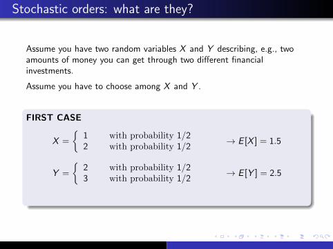
Stochastic orders: what are they?

Assume you have two random variables X and Y describing, e.g., twoamounts of money you can get through two different financialinvestments.

Assume you have to choose among X and Y .

FIRST CASE

{1 with probability 1/22 with probability 1/2

→ E [X ] = 1.5

→ E [Y ] = 2.5

Here Y is better than X .

FIRST CASE

→ E [X ] = 1.5

→ E [Y ] = 2.5

FIRST CASE

→ E [X ] = 1.5

→ E [Y ] = 2.5

FIRST CASE

→ E [X ] = 1.5

→ E [Y ] = 2.5

SECOND CASE

→ E [X ] = 1.5

→ E [Y ] = 1.5

Here X is better than Y (but nor for everybody, and not always).

THIRD CASE

X = 1 with probability 1 → E [X ] = 1

→ E [Y ] = 1.5

Here we can not immediately assert which one is the best choice.

SECOND CASE

→ E [X ] = 1.5

→ E [Y ] = 1.5

THIRD CASE

→ E [Y ] = 1.5

SECOND CASE

→ E [X ] = 1.5

→ E [Y ] = 1.5

THIRD CASE

→ E [Y ] = 1.5

SECOND CASE

→ E [X ] = 1.5

→ E [Y ] = 1.5

THIRD CASE

→ E [Y ] = 1.5

Thus, we have to introduce new criteria to choose among differentalternatives, taking into account our needs. → Stochastic orders

In fact, a long list of different stochastic orders have been defined, andapplied, in a variety of fields (economics and finance, engineering,medicine, etc.)

They are based on comparisons between:

• The location, or magnitude, of the random variables to be compared(mainly considered in reliability and survival analysis)

Ex: X is better than Y if P[X > t] ≥ P[Y > t] for all t ∈ R (usualstochastic order)

Thus, we have to introduce new criteria to choose among differentalternatives, taking into account our needs. → Stochastic orders

In fact, a long list of different stochastic orders have been defined, andapplied, in a variety of fields (economics and finance, engineering,medicine, etc.)

They are based on comparisons between:

• The location, or magnitude, of the random variables to be compared(mainly considered in reliability and survival analysis)

Ex: X is better than Y if P[X > t] ≥ P[Y > t] for all t ∈ R (usualstochastic order)

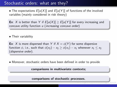
• The expectations E [u(X )] and E [u(Y )] of functions of the involvedvariables (mainly considered in risk theory)

Ex: X is better than Y if E [u(X )] ≥ E [u(Y )] for every increasing andconcave utility function u (increasing concave order)

• Their variability

Ex: X is more dispersed than Y if X = φ(Y ) for some dispersivefunction φ, i.e., such that φ(x2)− x2 ≥ φ(x1)− x1 whenever x1 ≤ x2(dispersive order).

• Moreover, stochastic orders have been defined in order to provide

comparisons in multivariate contexts;

comparisons of stochastic processes.

Stochastic comparisons of stochastic processes

• B.B. and Marco Scarsini. Convex orderings for stochasticprocesses. Comment. Math. Univ. Carolin. 32 (1991), no. 1, 115–118.

• B.B. and Marco Scarsini. On the comparison of pure jumpprocesses. RAIRO Rech. Oper. 26 (1992), no. 1, 41–55.

• B.B., Erhan Cinlar and Marco Scarsini. Stochastic comparisons ofIto processes. Stochastic Process. Appl. 45 (1993), no. 1, 1–11.

• B.B. and Marco Scarsini. Positive dependence orderings andstopping times. Ann. Inst. Statist. Math. 46 (1994), no. 2, 333–342.

Multivariate stochastic models

• B.B. and Fabio Spizzichino. Stochastic comparisons for residuallifetimes and Bayesian notions of multivariate ageing. Adv. in Appl.Probab. 31 (1999), no. 4, 1078–1094.

• B.B. and Fabio Spizzichino. Dependence and multivariate aging:the role of level sets of the survival function. System and Bayesianreliability, 229–242, Ser. Qual. Reliab. Eng. Stat., 5, World Sci. Publ.,2001.

• B.B., Subhash Kochar and Fabio Spizzichino. Some bivariate notionsof IFR and DMRL and related properties. J. Appl. Probab. 39(2002), no. 3, 533–544.

• B.B. and Fabio Spizzichino. Bivariate survival models with Claytonaging functions. Insurance Math. Econom. 37 (2005), no. 1, 6–12.

• B.B. and Fabio Spizzichino. Relations among univariate aging,bivariate aging and dependence for exchangeable lifetimes. J.Multivariate Anal. 93 (2005), no. 2, 313–339.

Lifetimes and stochastic orders

Let X and Y represent the lifetimes of two items, or individuals.

Recall: X is said to be smaller in the usual stochastic order than Y if andonly if P[X > t] ≤ P[Y > t] for all t ∈ R+, or, equivalently, if and onlyif E [φ(X )] ≤ E [φ(Y )] for every increasing function φ.

Apart the usual stochastic order, other comparisons are commonlyconsidered in survival analysis. In particular, different orders have beendefined and studied to compare residual lifetimes, i.e., to compare thevariables [X − t|X > t] and [Y − t|Y > t], for t ∈ R+.

Among them, the hazard rate order, the mean residual life order, thelikelihood ratio order, etc.

By means of these orders, it is possible to provide a list of alternativecharacterizations of aging, i.e., of the effect of the age in the residuallifetime of the items.

Ex: X has Increasing Hazard Rate (IHR) if[X − t1|X > t1] ≥st [X − t2|X > t2] for all 0 ≤ t1 ≤ t2, i.e., if theresidual lifetime of X stochastically decreases with the age.

Contributions by Bruno (and Fabio)

Analysis of lifetimes models and aging in multivariate contexts;

Criteria for the stochastic comparison of residual lifetimes based onsurvivals at different ages.

Thanks to their studies, now we have

A clear understanding of the effects of mutual dependencebetween items on their aging

A clear understanding of the relationships between univariateaging, multivariate aging and dependence

Ex: As a natural extension of the concept of univariate IHR aging to thebivariate case, one can consider the following:

• The random vector (X ,Y ) satisfies the Bivariate Increasing HazardRate (BIHR) property if, and only if, for all 0 ≤ t1 ≤ t2,

[(X−t1,Y−t1)|{X > t1,Y > t1}] ≥st [(X−t2,Y−t2)|{X > t2,Y > t2}].

• In a similar way, by reversing the inequality, one can define thecorresponding negative aging property Bivariate Decreasing Hazard Rate(BDHR).

• Let us say now that the lifetimes X and Y have positive dependence iflarge (respectively, small) values of X tend to go together (in somestochastic sense) with large (respectively, small) values of Y . Similarlydefine the negative dependence: if large (respectively, small) values of Xtend to go together (in some stochastic sense) with small (respectively,large) values of Y . [Formal definitions can be given by means of thecopula of the vector (X ,Y ).]

Bruno and Fabio formalized the following relationships (and similar ones).

positive dependence + univariate negative aging⇓

multivariate negative aging;

positive dependence + multivariate positive aging⇓

univariate positive aging;

multivariate positive aging + univariate negative aging⇓

negative dependence;

Bruno and Fabio formalized the following relationships (and similar ones).

positive dependence + univariate negative aging⇓

multivariate negative aging;

positive dependence + multivariate positive aging⇓

univariate positive aging;

multivariate positive aging + univariate negative aging⇓

negative dependence;

Recently....

Also, they shown, through counterexamples, but also clearly explainingwhy, we have

multivariate positive aging + univariate positive aging6⇓

positive dependence

Recently....

Also, they shown, through counterexamples, but also clearly explainingwhy, we have

multivariate positive aging + univariate positive aging6⇓

positive dependence

Recently....

Even if based on stochastic orders, Bruno and Fabio concentratedtheir studies on applications of comparisons in multivariate agingand survival models, without realizing the effects of their results inother fields. Like, for example, their possible applications in theanalysis of the properties of Joint Stochastic Orders.

Defined and studied for the first time by Shantikumar and Yao(1991), Bivariate characterization of some stochastic order relations.Adv. in Appl. Prob., 23, 642–659, the joint stochastic orders havebeen introduced in order to compare, marginally, univariate lifetimes,but taking into account their possible mutual dependence.

Recently....

Even if based on stochastic orders, Bruno and Fabio concentratedtheir studies on applications of comparisons in multivariate agingand survival models, without realizing the effects of their results inother fields. Like, for example, their possible applications in theanalysis of the properties of Joint Stochastic Orders.

Defined and studied for the first time by Shantikumar and Yao(1991), Bivariate characterization of some stochastic order relations.Adv. in Appl. Prob., 23, 642–659, the joint stochastic orders havebeen introduced in order to compare, marginally, univariate lifetimes,but taking into account their possible mutual dependence.

Recently....

Ex: Consider a pair (X ,Y ) of non-independent lifetimes. It is possible tocompare the corresponding residual lifetimes considering the inequalities[X − t|X > t] ≤st [Y − t|Y > t] for all t ∈ R+ (hazard rate order, ≤hr ).This is a comparison based on the marginal distributions of X and Y .

Otherwise, it is possible to compare their residual lifetimes taking intoaccount survivals of both, i.e., consider the following inequalities:

[X − t|{X > t,Y > t}] ≤st [Y − t|{X > t,Y > t}] for all t ∈ R+.

This is a joint stochastic order based on the joint distribution of (X ,Y )(joint weak hazard rate order, ≤hr :wj).

It can be shown that the stochastic orders above are not equivalent, i.e.,

X ≤hr Y 6⇔ X ≤wj :hr Y .

Actually, the equivalence holds if, and only if, X and Y are independent.

Recently....

Because of its properties, the joint weak hazard rate order has interestingapplications is different fields, like in reliability (optimal allocation ofcomponents), in actuarial sciences, in portfolio theory or in medicine(crossover clinical trials).

Ex: Let (X ,Y ) be such that X ≤hr :wj Y . It can be shown that in thiscase

E [g(X ,Y )] ≥ E [g(Y ,X )]

for all function g : R2 → R such that

∆g(x , y) = g(x , y)− g(y , x)

is supermodular in the set U = {(x , y) ∈ R2, x ≥ y}.

Recently....

Because of its properties, the joint weak hazard rate order has interestingapplications is different fields, like in reliability (optimal allocation ofcomponents), in actuarial sciences, in portfolio theory or in medicine(crossover clinical trials).

Ex: Let (X ,Y ) be such that X ≤hr :wj Y . It can be shown that in thiscase

E [g(X ,Y )] ≥ E [g(Y ,X )]

for all function g : R2 → R such that

∆g(x , y) = g(x , y)− g(y , x)

is supermodular in the set U = {(x , y) ∈ R2, x ≥ y}.

Recently....

Consider now a pair (X ,Y ) of non-independent financial returns, andconsider the two portfolios

Z1 = αY + (1− α)X and Z2 = (1− α)Y + αX , α ∈ [0, 1].

Because of the previous property, for α ≥ 1/2 one has

X ≤hr :wj Y =⇒ E [u(Z1)] ≥ E [u(Z2)]

for every logarithmic utility function u (like, e.g., u(t) = ln(1 + t)).

[The proof easily follows letting g(x , y) = u(αy + (1− α)x).]

Another interesting property of the joint weak hazard rate order is that itis closed with respect to mixtures (while the standard hazard rate order isnot)

Recently....

Z1 = αY + (1− α)X and Z2 = (1− α)Y + αX , α ∈ [0, 1].

X ≤hr :wj Y =⇒ E [u(Z1)] ≥ E [u(Z2)]

Recently....

Z1 = αY + (1− α)X and Z2 = (1− α)Y + αX , α ∈ [0, 1].

X ≤hr :wj Y =⇒ E [u(Z1)] ≥ E [u(Z2)]

Recently....

Studying the properties of this particular order, we verified that arelationship between the joint weak hazard rate order and the standardhazard rate order can be stated by making use of a notion defined andanalyzed by Bruno and Fabio in their works.

Definition

A bivariate copula C : [0, 1]2 −→ [0, 1] is called supermigrative(submigrative) if it is symmetric, i.e. C (u, v) = C (v , u) for every(u, v) ∈ [0, 1]2, and it satisfies

C (u, γv) ≥ (≤) C (γu, v)

for all u ≤ v and γ ∈ (0, 1).

Recently....

Studying the properties of this particular order, we verified that arelationship between the joint weak hazard rate order and the standardhazard rate order can be stated by making use of a notion defined andanalyzed by Bruno and Fabio in their works.

Definition

A bivariate copula C : [0, 1]2 −→ [0, 1] is called supermigrative(submigrative) if it is symmetric, i.e. C (u, v) = C (v , u) for every(u, v) ∈ [0, 1]2, and it satisfies

C (u, γv) ≥ (≤) C (γu, v)

for all u ≤ v and γ ∈ (0, 1).

Recently....

As shown by Bruno and Fabio, examples of copulas satisfying thesupermigrative property are the Archimedean ones having log-convexinverse generators. Thus, e.g., the Gumbel-Hougaard copula, and theFrank and Clayton copulas with positive value of the parameter θ. TheFarlie-Gumbel-Morgenstern copula, with posite value of the parameter,satisfies this property as well.

Recently....

It can be shown that the following holds.

Theorem

Let the survival copula C (X ,Y ) of (X ,Y ) be supermigrative. Then

X ≤hr Y =⇒ X ≤hr :wj Y . Viceversa, if the survival copula C (X ,Y ) of(X ,Y ) is submigrative, then X ≤hr :wj Y =⇒ X ≤hr Y .

Recently....

It can be shown that the following holds.

Theorem

Let the survival copula C (X ,Y ) of (X ,Y ) be supermigrative. Then

X ≤hr Y =⇒ X ≤hr :wj Y . Viceversa, if the survival copula C (X ,Y ) of(X ,Y ) is submigrative, then X ≤hr :wj Y =⇒ X ≤hr Y .

A final remark

Results similar to the previous one can be proved also for the otherwell-know joint orders.

Definition

Let D be the set of functions D = {g | g : R2 → R}. We denote:

Ghr = {g ∈ D | g(x , y)− g(y , x) is non-decreasing in x ∀y ≤ x};Glr = {g ∈ D | g(x , y) ≥ g(y , x) for all y ≤ x}.

Definition

Given two random variables X and Y as above, X is said to be greaterthan Y

in the joint hazard rate order (denoted X ≥hr :j Y ) ifE [g(X ,Y )] ≥ E [g(Y ,X )] for all g ∈ Ghr ;in the joint likelihood ratio order (denoted X ≥lr :j Y ) ifE [g(X ,Y )] ≥ E [g(Y ,X )] for all g ∈ Glr .

A final remark

Definition

A final remark

Definition

A final remark

Recall the definition of standard joint likelihood ratio:

X ≥lr Y ⇐⇒ [X − t| t ≤ X ≤ t + s] ≥st [Y − t| t ≤ Y ≤ t + s]

for all t ∈ R, s ∈ R+.

Theorem

Let (X ,Y ) be a random vector with an absolutely continuous survival

copula C(X ,Y ). Assume that

C(X ,Y ) is exchangeable (symmetric);

The density c(X ,Y )(u, v) is non-increasing in u and non-decreasing inv for all u ≥ v.

Then X ≥lr [≥hr ] Y implies X ≥lr :j [≥hr :j ] Y .

A final remark

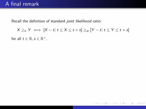
Recall the definition of standard joint likelihood ratio:

X ≥lr Y ⇐⇒ [X − t| t ≤ X ≤ t + s] ≥st [Y − t| t ≤ Y ≤ t + s]

for all t ∈ R, s ∈ R+.

Theorem

Let (X ,Y ) be a random vector with an absolutely continuous survival

copula C(X ,Y ). Assume that

C(X ,Y ) is exchangeable (symmetric);

The density c(X ,Y )(u, v) is non-increasing in u and non-decreasing inv for all u ≥ v.

Then X ≥lr [≥hr ] Y implies X ≥lr :j [≥hr :j ] Y .

A final remark

The second assumption appearing in this statement has an immediateinterpretation: it essentially means that for every point (u, v) below thediagonal and for any point (u, v) contained in the closed triangle withvertices (u, v), (u, u) and (v , v) it holds c(X ,Y )(u, v) ≥ c(X ,Y )(u, v) (andsimilarly for points above the diagonal).

A final remark

Roughly speaking, it is satisfied by copulas having probability massmainly concentrated around the diagonal, thus describing positivedependence, as the copulas having density uniformly distributed onregions like the ones shown in the following figure.

Such an assumption can be further weakened in order to let the relationX ≥lr Y ⇒ X ≥lr :j Y be satisfied also for survival copulas having asingularity on the diagonal v = u, like Cuadras-Auge copulas or Frechetcopulas.

A larger class of copulas satisfying this property has been defined andstudied in Durante (2006), A new class of symmetric bivariate copulas, Jof Nonparametrical Statistics, 18, 499–510.

A final remark

stochastic orders: a brief introduction and bruno’s contributions. · franco pellerey. stochastic...

Documents