stochastic modelling of structural elements -...

Chapter 5

© 2012 Opeyemi, licensee InTech. This is an open access chapter distributed under the terms of the Creative Commons Attribution License (http://creativecommons.org/licenses/by/3.0), which permits unrestricted use, distribution, and reproduction in any medium, provided the original work is properly cited.

Stochastic Modelling of Structural Elements

David Opeyemi

Additional information is available at the end of the chapter

http://dx.doi.org/10.5772/45951

1. Introduction

One of the primary goals of structural engineers is to assure proper levels of safety for the structures they design. This seemingly simple task is complicated by uncertainties associated with the materials with which the structure was designed and the loads they must resist, as well as our inaccuracies in analysis and design. Structural reliability and probabilistic analysis/design are tools which can be employed to quantify these uncertainties and inaccuracies, and produce designs and design procedures meeting acceptable levels of safety. Recent researches in the area of structural reliability and probabilistic analysis have centred on the development of probability-based design procedures. These include load modelling, ultimate and service load performance and evaluation of current levels of safety/reliability in design (Farid Uddim, 2000; Afolayan, 1999; Afolayan, 2003; Afolayan and Opeyemi, 2008; Opeyemi, 2009).

Deterministic methods are very subjective and are generally not based on a systematic assessment of reliability, especially when we consider their use in the entire structure. These methods can produce structures with some “over designed” components and perhaps some “under designed” components. The additional expense incurred in constructing the over designed components probably does not contribute to the overall reliability of the structure, so this is not a very cost-effective way to produce reliable structures. In other words, it would be better to redirect some of the resources used to build the over designed components toward strengthening the under designed ones. Therefore, there is increasing interest in adopting reliability-based design methods in civil engineering. These methods are intended to quantify reliability, and thus may be used to develop balance designs that are both more reliable and less expensive. Also, according to Coduto (2001), the methods can be used to better evaluate the various sources of failure and use this information to develop design and construction methods that are both more reliable and more robust - one that is insensitive to variations in materials, construction techniques, and environment.

Stochastic Modeling and Control 82

The reliability of an engineering system can be defined as its ability to fulfil its design purpose for some time period. The theory of probability provides the fundamental basis to measure this ability. The reliability of a structural element can be viewed as the probability of its satisfactory performance according to some performance functions under specific service and extreme conditions within a stated time period. In estimating this probability, system uncertainties are modelled using random variables with mean values, variances, and probability distribution functions. Many methods have been proposed for structural reliability assessment purposes, such as First Order Second Moment (FOSM) method, Advanced Second Moment (ASM) method, and Computer-based Monte Carlo Simulation (MCS) (e.g., Ang and Tang,1990;Ayyub and Haldar,1984; White and Ayyub,1985; Ayyub and McCuen,1997) as reported by Ayyub and Patev (1998).

The concept of the First-Order Reliability Method (FORM) is a powerful tool for estimating nominal probability level of failure associated with uncertainties and it is the method adopted for the reliability estimations in this text. The general problem to which FORM provides an approximate solution is as follows. The state of a system is a function of many variables some of which are uncertain. These uncertain variables are random

with joint distribution function 1

( ) ( { })n

x i ii

F x P X x

defining the stochastic model. For

FORM, it is required that XF (x), is at least locally continuously differentiable, i. e., that

probability densities exist. The random variables 1( ,... )TnX X X are called basic variables.

The locally sufficiently smooth (at least once differentiable) state function is denoted by g(X). It is defined such that g(X)>0 corresponds to favourable (safe, intact, acceptable) state. g(X) =0 denotes the so-called limit state or the failure boundary. Therefore, g(X) <0 (sometimes also g(X) ≤ 0) defines the failure (unacceptable, adverse) domain, F. The function g(X) can be defined as an analytic function or an algorithm (e.g., a finite element code). In the context of FORM it is convenient but necessary only locally that g(X) is a monotonic function in each component of X. Among other useful information FORM produces an approximation to:

( ) 0

( ) ( ( ) 0) ( ) ( )f X Rg x

P P X F P g X dF x

(1)

In which βR = the reliability or safety index (Melchers, 2002).

Mathematical models, be they deterministic or stochastic, are intended to mimic real world systems. In particular, they can be used to predict how systems will behave under specified conditions. In scientific work, we may be able to conduct experiments to see if model predictions agree with what actually happens in practice. But in many situations, experimentation is impossible. Even if experimentation is conceivable in principle, it may be impractical for ethical or financial reasons. In these circumstances, the model can only be tested less formally, for example by seeking expert opinion on the predictions of the model.

Stochastic Modelling of Structural Elements 83

The examples based on the author’s research work introduce a different collection of stochastic models on analysis of the carrying capacities of piles based on static and dynamic approaches with special consideration to steel and precast concrete as pile types in cohesive, cohesionless, and intermediate soils between sand and clay and layered soils. Steel and precast concrete piles were analysed based on static pile capacity equations under various soils such as cohesive, cohesionless, and intermediate soils between sand and clay and layered soils. Likewise, three (3) dynamic formulae, namely: Hiley, Janbu and Gates were closely examined and analysed using the first-order reliability concept (Afolayan and Opeyemi, 2008; Opeyemi, 2009).

2. General methods and procedures for modelling structural elements

Structural reliability is concerned with the calculation and prediction of the probability of limit state violation for an engineered structural system at any stage during its life. In particular, the study of structural safety is concerned with violation of the ultimate or safety limit states for the structure. In probabilistic assessments any uncertainty about a variable expressed in terms of its probability density function is taken into account explicitly. This is not the case in traditional ways of measuring safety, such as the “factor of safety” or “load factor”. These are “deterministic” measures since the variables describing the structure; its strength and the applied loads are assumed to take on known (if conservative) values about which there are assumed to be no uncertainty. The loads which are applied to a structure fluctuate with time and are of uncertain value at any one point in time. This is carried over directly to the load effects (or internal actions) S. Somewhat similarly the structural resistance R will be a function of time (but not a fluctuating one) owing to deterioration and similar actions. Loads have a tendency to increase, and resistances to decrease, with time. It is usual also for the uncertainty in both these quantities to increase with time. This means that the probability density functions fS ( ) and fR ( ) become wider and flatter with time and that the mean values of S and R also change with time. The safety limit state will be violated whenever, at any time t.

( )( ) – ( ) 0 or 1( )

R tR t S tS t

(2)

The probability that this occurs for any one load application (or load cycle) is the probability of limit state violation, or simply the probability of failure Pf.

2.1. Reliability analysis

For basic structural reliability problem only one load effect S resisted by one resistance R is considered. Each described by a known probability density function FS( ) and FR( ) respectively. S is obtained from the applied loading Q through a structural analysis, but R and S are expressed in the same units.


For convenience, but without loss of generality, only the safety of a structural element is considered and as usual, that structural element will be considered to have failed if its resistance R is less than the stress resultant S acting on it. The probability of failure, Pf of the structural element will be stated as follows:

Pf = P (G (R, S) 0) (3)

Where G ( ) is termed the “limit state function” and the probability of failure is identical with the probability of limit state violation.

In general, R is a function of material properties and element or structure dimensions, while S is a function of applied loads Q, material densities and perhaps dimensions of the structure, each of which may be a random variable. Also, R and S may not be independent, such as when some loads act to oppose failure (e.g. overturning) or when

f R sP P R – S 0 F x f x dx

(4)

2.1.1. Modeling procedures

The first step is to define the variables involved in the generalized reliability problem. The fundamental variables which define and characterize the behaviour and safety of a structure, termed “basic” variables, usually are variables employed in conventional structure analysis and design. Examples are dimensions densities or unit weights, materials, loads, material strengths, etc. It is very convenient to choose the basic variables such that they are independent, since dependence between basic variables usually adds some complexity to a reliability analysis.

The probability distributions will then be assigned to the basic variables, depending on the knowledge that is available. If it can be assumed that past observations and experience for similar structure can be used, validly, for the structure under consideration the probability distributions might be inferred directly from such observed data. More generally, subjective information may be employed or some combination of techniques is required. Sometimes physical reasoning may be used to suggest an appropriate probability distribution.

The parameters of the distribution are estimated from the data by using one of the usual methods viz: methods of moments, maximum likelihood, or order statistics.

Finally, when the model parameters have been selected, the model would be compared with the data. A graphical plot on appropriate probability paper is often very revealing, but analytical “goodness of fit” tests could be used also.

When or after the basic variables and their probability distributions have been established, the next step is to replace the simple R – S form of limit state function with a generalized version expressed directly in terms of basic variables.


The vector X will be used to represent all the basic variables involved in the problem. Then the resistance R will be expressed as R – GR(X) and the loading or load effect as S = GS(X). The limit state function G (R, S) can be generalized. When the functions GR(X) and GS(X) are used in G (R,S), the resulting limit state function will be written simply as G(X), where X is the vector of all relevant basic variables and G( ) is some function expressing the relationship between the limit state and the basic variables.

The limit state equation G(x) = 0 now defines the boundary between the satisfactory or ‘safe’ domain G>0 and the unsatisfactory or ‘unsafe’ domain G≤O in n-dimensional basic variable space.

Figure 1. The n-dimensional basic variable space.

With the limit state function expressed as G(x), the generalization of

f RSP P R – S 0 f r,s dr dsD

(5)

Becomes


f x( ) 0

P P G x 0 f x dxG x

(6)

Sidestepping the integration process completely by transforming fx(x) in (6) to a multi-normal probability density function and using some remarkable properties which may then be used to determine, approximately, the probability of failure – the so-called ‘First Order Second Moment’ methods.

Rather than use approximate (and numerical) methods to perform the integration required in the reliability integral; the probability density function fx ( ) in the integrand is simplified. In this case the reliability estimation with its each variable is represented only by its first two moments i.e. by its mean and standard deviation. This is known as the “Second – Moment” level of representation. A convenient way in which the second-moment representation might be interpreted is that each random variable is represented by the normal distribution. This continuous probability distribution is described completely by its first two moments.

Because of their inherent simplicity, the so-called “Second-moment” methods have become very popular. Early works by Mayer (1926), Freudenthal (1956), Rzhanitzyn (1957) and Basler (1961) contained second moment concepts. Not until the late 1960s, however, was the time ripe for the ideas to gain a measure of acceptance, prompted by the work of Cornell (1969) as reported by Melchers (1999).

When resistance R and load effects are each Second-moment random variables (i.e. such as having normal distributions), the limit state equation is the “safety margin” Z = R – R and the probability of failure Pf is

( ) zf

z

UP

(7)

Where β is the (simple) ‘safety’ (or ‘reliability’) index and φ( ) the standard normal distribution function.

2.1.2. First Order Reliability Method (FORM)

FORM has been designed for the approximate computation of general probability integrals over given domains with locally smooth boundaries but especially for probability integrals occurring in structural reliability. Similar integrals are also found in many other areas, for example, in hydrology, mathematical statistics, control theory, classical hardware reliability and econometrics which are the areas where FORM has already been applied.

The concept of FORM is, essentially, based on

f E X( ) 0

P P X F P g X 0 dF xG x

(8)


3. Example applications

Some examples are hereby introduced to show particular cases of stochastic modelling as applied to the study of structural analysis of the carrying capacities of piles based on static and dynamic approaches with special consideration to steel and precast concrete as pile types in cohesive, cohesionless, and intermediate soils between sand and clay and layered soils, taken from the author’s experience in research in the structural and geotechnical engineering field. Steel and precast concrete piles were analyzed based on static pile capacity equations under various soils such as cohesive, cohesionless, and intermediate soils between sand and clay and layered soils. Likewise, three (3) dynamic formulae (namely: Hiley, Janbu and Gates) were closely examined and analyzed using the first-order reliability concept.

Pile capacity determination is very difficult. A large number of different equations are used, and seldom will any two give the same computed capacity. Organizations which have been using a particular equation tend to stick to it especially when successful data base has been established. It is for this reason that a number of what are believed to be the most widely used (or currently accepted) equations are included in most literature.

Also, the technical literature provides very little information on the structural aspects of pile foundation design, which is a sharp contrast to the mountains of information on the geotechnical aspects. Building codes present design criteria, but they often are inconsistent with criteria for the super structure, and sometimes are incomplete or ambiguous. In many ways this is an orphan topic that neither structural engineers nor geotechnical engineers have claimed as their own.

3.1. Static pile capacity of concrete piling in cohesive soils

The functional relationship between the allowable design load and the allowable pile capacity can be expressed as follows:

G(X) = Allowable Design Load – Allowable Pile Capacity,

So that,

2 2 21 2 1

1

2 2 21 2 1 1

( ) 0.33 0.4 { (9 ) } /4 4 4

0.259 0.314 - 7.07 3.142

cu y u b u

ycu u b u

D D DG X f f S D L S SF

f D f D D S D L S SF

(9)

In which fcu= characteristic strength of concrete, D1= pile diameter, D2= steel diameter, fy = characteristic strength of steel, Su= cohesion, Lb= pile length, α= adhesion factor, and SF=factor of safety.


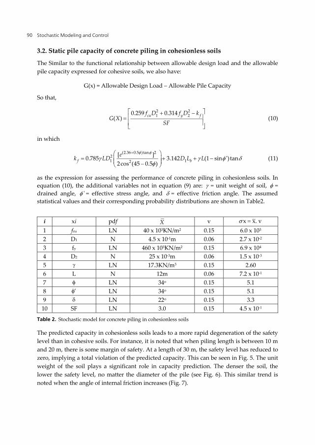
i xi pdf x v x x. v 1 fcu LN 40 x 103 0.15 6.0 x 103 2 D1 N 3 x 10-1m 0.06 1.8 x 10-2 3 fy LN 460 x

103KN/m2 0.15 6.9 x 104

4 D2 N 25 x 10-3m 0.06 1.5 x 10-3 5 Su LN 12KN/m2 0.15 1.8 6 LN 1.00 0.15 1.5 x 10-1 7 Lb N 23.0m 0.06 1.38 8 SF LN 3.0 0.15 4.5 x 10-1

Table 1. Stochastic model for concrete piling in cohesive soils.

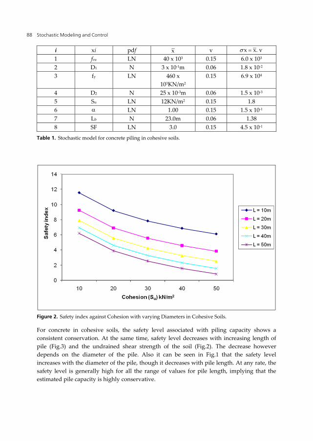
Figure 2. Safety index against Cohesion with varying Diameters in Cohesive Soils.

For concrete in cohesive soils, the safety level associated with piling capacity shows a consistent conservation. At the same time, safety level decreases with increasing length of pile (Fig.3) and the undrained shear strength of the soil (Fig.2). The decrease however depends on the diameter of the pile. Also it can be seen in Fig.1 that the safety level increases with the diameter of the pile, though it decreases with pile length. At any rate, the safety level is generally high for all the range of values for pile length, implying that the estimated pile capacity is highly conservative.


Figure 3. Safety index against Length of Pile with varying Diameters in Cohesive Soils.

Figure 4. Safety index against Factor of Safety with varying Lengths

0

2

4

6

8

10

12

14

10 20 30 40 50

Length of Pile

Safe

ty in

dex

D = 200mm

D = 300mm

D = 400mm

D = 500mm

D = 600mm


3.2. Static pile capacity of concrete piling in cohesionless soils

The Similar to the functional relationship between allowable design load and the allowable pile capacity expressed for cohesive soils, we also have:

G(x) = Allowable Design Load – Allowable Pile Capacity

So that,

2 21 20.259 0.314

( ) cu y ff D f D kG X

SF

(10)

in which

(2.36 0.5 ) tan 2

21 12

[ ]0.785 3.142 (1 sin ') tan2cos (45 0.5 )f bek LD D L L

(11)

as the expression for assessing the performance of concrete piling in cohesionless soils. In equation (10), the additional variables not in equation (9) are: = unit weight of soil, = drained angle, ' = effective stress angle, and = effective friction angle. The assumed statistical values and their corresponding probability distributions are shown in Table2.

i xi pdf X v x x. v 1 fcu LN 40 x 103KN/m2 0.15 6.0 x 103 2 D1 N 4.5 x 10-1m 0.06 2.7 x 10-2 3 fy LN 460 x 103KN/m2 0.15 6.9 x 104 4 D2 N 25 x 10-3m 0.06 1.5 x 10-3 5 LN 17.3KN/m3 0.15 2.60 6 L N 12m 0.06 7.2 x 10-1 7 LN 34o 0.15 5.1 8 LN 34o 0.15 5.1 9 LN 22o 0.15 3.3

10 SF LN 3.0 0.15 4.5 x 10-1

Table 2. Stochastic model for concrete piling in cohesionless soils

The predicted capacity in cohesionless soils leads to a more rapid degeneration of the safety level than in cohesive soils. For instance, it is noted that when piling length is between 10 m and 20 m, there is some margin of safety. At a length of 30 m, the safety level has reduced to zero, implying a total violation of the predicted capacity. This can be seen in Fig. 5. The unit weight of the soil plays a significant role in capacity prediction. The denser the soil, the lower the safety level, no matter the diameter of the pile (see Fig. 6). This similar trend is noted when the angle of internal friction increases (Fig. 7).


Figure 5. Safety index against Length of Pile with varying Diameters

Figure 6. Safety index against Unit weight of soil with varying Diameters


Figure 7. Safety index against Angle of internal friction with varying Diameters

3.3. Static pile static pile capacity of steel piling in cohesive soils


0.35 -y p p u s uf A A qS A S SF

0.35 -y p u p sf A S qA A SF (12)

i xi pdf X v x = X . v 1 Fy LN 460 x 103KN/m2 0.15 6.9 x 104 2 Ap N 1.4 x 10-1 m2 0.06 8.4 x 10-3 3 Su LN 28 KN/m2 0.15 4.2 4 LN 1.00 0.15 1.5 x 10-1 5 As N 48.84 m2 0.06 2.93 6 SF LN 2.0 0.15 3.0 x 10-1

Table 3. Stochastic model for steel piling in cohesive soils.


Figure 8. Safety index against Cohesion with varying Pile areas

Figure 9. Safety index against Adhesive factor with varying Pile areas


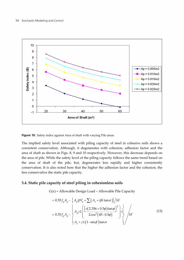
Figure 10. Safety index against Area of shaft with varying Pile areas

The implied safety level associated with piling capacity of steel in cohesive soils shows a consistent conservation. Although, it degenerates with cohesion, adhesion factor and the area of shaft as shown in Figs. 8, 9 and 10 respectively. However, this decrease depends on the area of pile. While the safety level of the piling capacity follows the same trend based on the area of shaft of the pile, but, degenerates less rapidly and higher consistently conservation. It is also noted here that the higher the adhesion factor and the cohesion, the less conservative the static pile capacity.

3.4. Static pile capacity of steel piling in cohesionless soils


2

2

0.35 - tan

2.356 0.5 tan

0.35 - 2cos 45 - 0.5

1 - sin tan

y p p q s

py p

s

f A A qN A qK SF

eA L

f A SF

A L

(13)


i xi pdf X v x x. v

1 Fy LN 460 x 103KN/m2 0.15 6.9 x 104

2 Ap N 1.60 x 10-1 m2 0.06 9.6 x 10-3

3 LN 17.3KN/m3 0.15 2.60

4 L N 12m 0.06 7.2 x 10-1

5 LN 34o 0.15 5.1

6 As N 16.96 m2 0.06 1.02

7 LN 34o 0.15 5.1

8 LN 22o 0.15 3.3

9 SF LN 3.0 0.15 4.5 x 10-1

Table 4. Stochastic model for steel piling in cohesionless soils.

Figure 11. Safety index against Angle of internal friction with varying Lengths

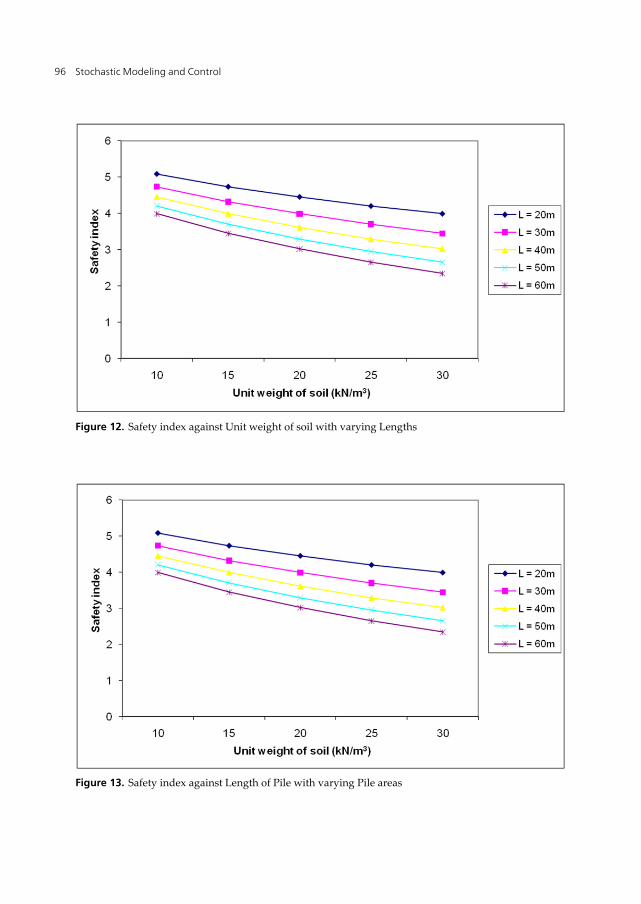
Piling reliability/safety level decreases as pile length, unit weight of soil and the angle of internal friction increases (Figs.11, 12 and 13) but the rate of decrease is more rapid for precast concrete than steel. For concrete piling, pile length greater than 30 m will result in catastrophe while much longer steel piles that economy will permit are admissible.


Figure 12. Safety index against Unit weight of soil with varying Lengths

Figure 13. Safety index against Length of Pile with varying Pile areas


3.5. Dynamic pile capacity using Hiley, Janbu and Gates formulae

Estimating the ultimate capacity of a pile while it is being driven in the ground at the site has resulted in numerous equations being presented to the engineering profession. Unfortunately, none of the equations is consistently reliable or reliable over an extended range of pile capacity. Because of this, the best means for predicting pile capacity by dynamic means consists in driving a pile, recording the driving history, and load testing the pile. It would be reasonable to assume that other piles with a similar driving history at that site would develop approximately the same load capacity.

Dynamic formulae have been widely used to predict pile capacity. Some means is needed in the field to determine when a pile has reached a satisfactory bearing value other than by simply driving it to some predetermined depth. Driving the pile to a predetermined depth may or may not obtain the required bearing value because of normal soil variations both laterally and vertically.

3.5.1. Dynamic pile capacity using Hiley formula


2p

y pp1 2 3

W n Weh Eh0.35f A - SF1 W WS K K K2

2

py p

pu1 3

W n Weh Eh0.35f A - SFW WP L

S 0.5 K KAE

(14)

i xi pdf X v x = X . v 1 Fy LN 460 x 103KN/m2 0.15 6.9 x 104 2 Ap N 1.60 x 10-2 m2 0.06 9.6 x 10-4 3 eh N 0.84 0.06 5.04 x 10-2 4 Eh LN 33.12 KN/m 0.15 4.97 5 S LN 1.79 x 10-2 m 0.15 2.69 x 10-3 6 K1 LN 4.06 x 10-3 m 0.15 6.09 x 10-4 7 Pu LN 950KN 0.15 1.425 x 102 8 L N 12.18m 0.06 7.31 x 10-1 9 E LN 209 x 106 KN/m2 0.15 3.14 x 107 10 K3 LN 2.54 x 10-3 m 0.15 3.81 x 10-4 11 W Gumbel 80 KN 0.30 24 12 n LN 0.5 0.15 7.5 x 10-2 13 Wp LN 18.5 KN 0.15 2.775 14 SF LN 4.0 0.15 6.0 x 10-1

Table 5. Stochastic model for dynamic pile using Hiley formula.


3.5.2. Dynamic pile capacity using Janbu frmula


y pu

eh Eh0.35f A - SFK S

2

Py p

Pr

r

W eh EhL AES0.35f A - eh Eh 0.75 0.15 1 1 S SFWW 0.75 0.15W

(15)

i xi pdf X v x = X . v 1 Fy LN 460 x 103KN/m2 0.15 6.9 x 104 2 Ap N 1.60 x 10-2 m2 0.06 9.6 x 10-4 3 eh N 0.84 0.06 5.04 x 10-2 4 Eh LN 33.12 KN/m 0.15 4.97 5 Wp LN 18.5 KN 0.15 2.78 6 Wr Gumbel 35.58 KN 0.30 1.07 x 101 7 L N 12.18m 0.15 7.31 x 10-1 8 E LN 209 x 106 KN/m2 0.06 3.14 x 107 9 S LN 1.79 x 10-2 m 0.15 2.69 x 10-3 10 SF LN 6.0 0.15 9.0 x 10-1

Table 6. Stochastic model for dynamic pile using Janbu formula.

3.5.3. Dynamic pile capacity using Gates formula


y p0.35f A - a eh Eh b-logS SF

1

2y p0.35f A - a eh Eh b-logS SF

(16)

i xi pdf X v x = X . v 1 Fy LN 460 x 103KN/m2 0.15 6.9 x 104 2 Ap N 1.60 x 10-2 m2 0.06 9.6 x 10-4 3 a N 1.05 x 10-1 0.06 6.3 x 10-3 4 eh N 0.85 0.06 5.1 x 10-2 5 Eh LN 33.12 KNm 0.15 4.97 6 b N 2.4 x 10-3 m 0.06 1.44 x 10-4 7 S LN 1.79 x 10-2 m 0.15 2.69 x 10-3 8 SF LN 3.0 0.15 4.5 x 10-1

Table 7. Stochastic model for dynamic pile using Gates formula.


Figure 14. Safety index against Factor of safety using Hiley, Janbu and Gates formulae

Figure 15. Safety index against Area of pile using Hiley, Janbu and Gates formulae


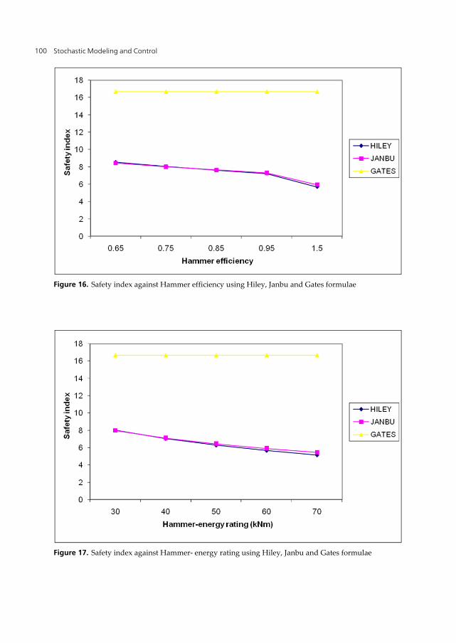
Figure 16. Safety index against Hammer efficiency using Hiley, Janbu and Gates formulae

Figure 17. Safety index against Hammer- energy rating using Hiley, Janbu and Gates formulae


The implied safety level associated with piling capacity using Gates’ formula is grossly conservative, even much more than Hiley and Janbu formulae. The safety level does not change with the area of pile, hammer efficiency and hammer-energy rating (Figs. 14 to 17). As is common in practice, the areas of piles, hammer efficiency, hammer energy rating and point penetration per blow are subjected to variations and the results of the assessment are as displayed in Figures 14 to 17.

Hiley formula generally and grossly provides a very conservative pile capacity as seen in Figs. 14 to 17. Nevertheless, the safety level does not change with area of pile (Fig. 15). As hammer efficiency and hammer energy rating increase, the safety level reduces significantly as in Fig. 16 and Fig.17 respectively. On the other hand, safety level grows with increasing factor of safety as normally expected (Fig. 14).

Just like the Hiley formula, Janbu formula leads to a grossly conservative pile capacity. However, Janbu’s prediction is not as conservative as Hiley’s with respect to hammer efficiency and hammer-energy rating. Generally Gates’ formula yields the most grossly conservative prediction compared to Hiley and Janbu. It is noted that safety level is not dependent on the area of pile, hammer efficiency and hammer-energy rating (Figs.14 to 17).

4. Conclusion

Reliability-based design methods could be used to address many different aspects of foundation design and construction. However, most of these efforts to date have focused on geotechnical and structural strength requirements, such as the bearing capacity of shallow foundations, the side friction and toe-bearing capacity of deep foundations, and the stresses in deep foundations. All of these are based on the difference between load and capacity, so we can use a more specific definition of reliability as being the probability of the load being less than the capacity for the entire design life of the foundation. Various methods are available to develop reliability-based design of foundations, most notably Stochastic methods, the First-Order Second-Moment Method, and the Load and Resistance Factor Design method.

Deterministic method is not a very cost-effective way to produce reliable structures; therefore, reliability-based design should be adopted to quantify reliability, and thus used to develop balance designs that are both more reliable and less expensive.

From all the preceding sections it is apparent how a stochastic modelling can contribute to the improvement of a structural design, as it can take into account the uncertainties that are present in all human projects.

Author details

David Opeyemi Rufus Giwa Polytechnic, Owo, Nigeria


Acknowledgement

I like to acknowledge my Supervisor, Professor J.O. Afolayan, for his guidance, teaching, patience, encouragement, suggestions and continued support, particularly for arousing my interest in Risk Analysis (Reliability Analysis of Structures).

5. References

Ayyub, B.M. and Patev, C.R. (1998).“Reliability and Stability Assessment of Concrete Gravity Structures”. (RCSLIDE): Theoretical Manual, US Army Corps of Engineers Technical Report ITL – 98 – 6.

Afolayan, J.O. (1999) “Economic Efficiency of Glued Joints in Timber Truss Systems”, Building and Environment: The International of Building Science and its Application, Vol. 34, No. 2, pp. 101 – 107.

Afolayan, J. O. (2003) “Improved Design Format for Doubly Symmetric Thin-Walled Structural Steel Beam-Columns”, Botswana Journal of Technology, Vol. 12, No.1, pp. 36 – 43

Afolayan, J. O. and Opeyemi, D.A. (2008) “Reliability Analysis of Static Pile Capacity of Concrete in Cohesive and Cohesionless Soils”, Research Journal of Applied Sciences, Vol.3, No. 5, pp. 407-411.

Bowles, J.E. (1988) Foundation Analysis and Design. 4th ed., McGraw-Hill Book Company, Singapore.

Coduto, D.P. (2001). Foundation Design: Principles and Practices. 2nd ed., Prentice Hall Inc., New Jersey.

Farid Uddin, A.K.M. (2000) “Risk and Reliability Based Structural and Foundation Design of a Water Reservoir (capacity: 10 million gallon) on the top of Bukit Permatha Hill in Malaysia”, 8th ASCE Specialty Conference on Probabilistic Mechanics and Structural Reliability.

Melchers, R.E. (2002). Structural reliability analysis and prediction, John Wiley & Sons, ISBN: 0-471-98771-9, Chichester, West Sussex, UK

Opeyemi, D.A. (2009) “Probabilistic Failure Analysis of Static Pile Capacity for Steel in Cohesive and Cohesionless Soils”, Electronic Journal of Geotechnical Engineering, Vol.14, Bund. F, pp. 1-12.

stochastic modelling of structural elements -...

Documents