stochastic modeling of single-hop cluster stability in...

0018-9545 (c) 2015 IEEE. Personal use is permitted, but republication/redistribution requires IEEE permission. Seehttp://www.ieee.org/publications_standards/publications/rights/index.html for more information.

This article has been accepted for publication in a future issue of this journal, but has not been fully edited. Content may change prior to final publication. Citation information: DOI10.1109/TVT.2015.2396298, IEEE Transactions on Vehicular Technology

1

Stochastic Modeling of Single-Hop Cluster Stabilityin Vehicular Ad Hoc Networks

Khadige Abboud, Student Member, IEEE, and Weihua Zhuang, Fellow, IEEE

Abstract—Node clustering is a potential approach to improvethe scalability of networking protocols in vehicular ad hocnetworks (VANETs). High relative vehicle mobility and frequentnetwork topology changes inflict new challenges on maintainingstable clusters. As a result, cluster stability is a crucial measureof the efficiency of clustering algorithms for VANETs. This paperpresents a stochastic analysis of the vehicle mobility impact onsingle-hop cluster stability. A stochastic mobility model is adoptedto capture the time variations of intervehicle distances (distanceheadways). Firstly, we propose a discrete-time lumped Markovchain to model the time variations of a system of distance head-ways. Secondly, the first passage time analysis is used to deriveprobability distributions of the time periods of invariant cluster-overlap state and cluster-membership as measures of clusterstability. Thirdly, queueing theory is utilized to model the limitingbehaviors of the numbers of common and unclustered nodesbetween neighbouring clusters. Numerical results are presentedto evaluate the proposed models, which demonstrate a closeagreement between analytical and simulation results.

I. INTRODUCTION

A vehicular ad hoc network (VANET) is a promising additionto our future intelligent transportation systems, which is provi-sioned to support various safety and infotainment applications[2], [3]. Urban roads and highways are highly susceptible to alarge number of vehicles and traffic jams. Therefore, network-ing protocols for VANETs should be scalable to support suchlarge scale networks. Node clustering is a network managementstrategy in which nearby nodes are grouped into a set calledcluster. In each cluster, a node, called cluster head (CH), iselected to manage the cluster. The remaining nodes are calledcluster members (CMs), each belonging to one or multipleclusters.

Node clustering, just as in traditional ad hoc networks, isa potential approach to improve the scalability of networkingprotocols such as for routing and medium access control inVANETs. For medium access control protocols, the CH canact as a central coordinator that manages the access of itsCMs to the wireless channel(s) [4]. For routing protocols, CHscan be made responsible for the discovery and maintenanceof routing paths, thus limiting the control-message overheadin these processes [5]. Despite the potential benefits of nodeclustering, forming and maintaining the clusters require explicitexchange of control messages. In VANETs, vehicles movewith high and variable speeds, causing frequent changes in thenetwork topology, which can significantly increase the clustermaintenance cost. Therefore, how to form stable clusters thatlast for a long time is a major issue in node clustering ofVANETs.

Copyright c©2015 IEEE. Personal use of this material is permitted. However,permission to use this material for any other purposes must be obtained fromthe IEEE by sending a request to [email protected].

K. Abboud and W. Zhuang are with the Center for Wireless Communications,Department of Electrical and Computer Engineering, University of Waterloo,200 University Avenue West, Waterloo, Ontario, Canada, N2L 3G1. E-mail:khabboud, [email protected]

This work is presented in part in a paper at the 2014 ACM MSWiM [1].

In a highly dynamic VANET, vehicles join and leave clustersalong their travel route, resulting in changes in cluster structure.The temporal changes in cluster structure are either internalor external [6]. An internal change in the cluster structureis concerned with a change inside the cluster such as whenvehicles join or leave the cluster, resulting in a change incluster-membership. Frequent changes in the internal clusterstructure consume network radio resources and cause servicedisruption for the cluster-based network protocols (e.g., inintracluster resource allocation, route discovery, and messagedelivery). Therefore, analyzing the impact of vehicle mobilityon the rate at which nodes enter and leave a cluster is animportant measure of internal cluster stability. This metric hasbeen adopted by researchers to evaluate the performance oftheir proposed clustering algorithms through simulations [7]–[9]. A higher rate of cluster-membership changes indicatesa smaller time period of invariant cluster-membership and,therefore, lower internal cluster stability.

On the other hand, an external change in the cluster structureis concerned with the relationship of a cluster with otherclusters in a network. One metric that evaluates the externalrelationship of a cluster is its overlapping ranges with neigh-boring clusters. The time variations of the distance betweentwo neighboring CHs, due to vehicle mobility, can cause thecoverage ranges of the clusters to overlap. As the overlappingrange between two clusters increases, the two clusters maymerge into a single cluster [4], [7], [10]. Frequent splitting andmerging of clusters increase the control overhead and drain theradio resources [9], [11], [12]. In general, a non-overlappingclustered structure produces a less number of clusters and low-ers the design complexity of network protocols that run on theclusters. For example, two clusters may utilize the same radioresources at the same time if they are non neighboring clusters[13] [14]. On the other hand, a highly overlapping clusteredstructure may cause complexity in the channel assignment,lead to broadcast storms, and form long hierarchical routes.Additional radio resources ought to be used to prevent inter-cluster interference due to overlapping, for example, assigningdifferent time frames for neighboring clusters [15] and assign-ing different transmission codes to CMs located in a possiblyoverlapping region [16]. Although researchers have favoredforming non-overlapping (or reduced overlapping) clusteredstructure [12] [11] [10] [16], encountering overlapping clustersduring the network runtime is inevitable, especially in a highlymobile network. Overlapping clusters have received significantattention since the work by Palla et al. [17]. It is shown thatreal networks are better characterized by well-defined statisticsof overlapping and nested clusters rather than disjoint clusters.Additionally, overlapping structure can provide a ground forcooperation among the overlapping clusters. For example, in[18], overlapping is used for cooperative interference manage-ment for small cell networks. Regardless of whether or notcluster overlapping is preferred, characterizing the overlappingstate between neighboring clusters and its changes over timebecomes crucial in the presence of node mobility. A higher rate



2

of cluster-overlap state change indicates a shorter time period ofunchanged cluster-overlap state and, therefore, lower externalcluster stability.

Despite the importance of cluster stability as a measureof clustering algorithm efficiency in VANETs, characterizingcluster stability has taken the form of simulations [7]–[9] orcase studies [19] in the literature.

In this paper, we present a stochastic analysis of two clusterstability metrics: the change rate in the overlap state betweenneighboring clusters as a measure of external cluster stabilityand the change rate in cluster-membership as a measure ofinternal cluster stability. We adopt a stochastic vehicle mo-bility model that describes the time variations of intervehicledistances and accounts for the realistic dependency of thesevariations at consecutive time steps. Firstly, the distance be-tween two vehicles, separated by a number of vehicles on ahighway, is modeled as a discrete-time Markov chain with areduced dimensionality. Using the first passage time analysis,we derive the probability distributions of the time before thefirst change in the cluster-overlap state and the time intervalbetween two successive changes in cluster-overlap state of twoneighboring clusters. Secondly, the distributions of the timebefore the first cluster-membership change and the time in-terval between two successive cluster-membership changes arederived. Thirdly, the overlapping region between overlappingclusters and the unclustered region between non-overlappingclusters are modeled as a storage buffer in a two-state randomenvironment. Using G/G/1 queuing theory, the steady-statedistributions of the numbers of common and unclustered nodesare approximated. Finally, we conduct MATLAB simulationsand demonstrate that the analytical results of our model matchwell with the simulation results.

II. SYSTEM MODEL

Consider a connected VANET on a multi-lane highway withno on or off ramps. We focus on a single lane with lane changesimplicitly captured in the adopted mobility model. We choose asingle lane from a multi-lane highway instead of a single-lanehighway, in order to be more realistic in a highway scenario.Assume that the highway is in a steady traffic flow conditiondefined by a time-invariant intermediate vehicle density. All thevehicles have the same transmission range, denoted by R. Anytwo nodes at a distance less than R from each other are one hopneighbours. Time is partitioned with a constant step size. LetXi be the distance headway between node i and node i + 1.The distance headway is the distance between two identicalpoints on two consecutive vehicles on the same lane. DefineXi = Xi(m),m = 0, 1, 2 . . . to be a discrete-time stochasticprocess of the ith distance headway, where Xi(m) is a randomvariable representing the distance headway of node i at themth time step, i = 0, 1, 2, . . . ,m = 0, 1, 2, . . . . Furthermore,assume that Xi’s are independent with identical statisticalbehaviors for all i ≥ 0. For notation simplicity, we omit indexi when referring to an arbitrary distance headway. Throughoutthis paper, FY (y), PY (y), and E[Y ] are used to denote thecumulative distribution function (cdf), the probability massfunction (pmf), and the expectation of random variable Y ,respectively.

A. Node ClustersWe assume that CHs are selected according to some clus-

tering scheme, so that all the network nodes are grouped into

CH

R

CM

0X

Xc

1X

2X

3X

CH

R

4X

Overlapping

range

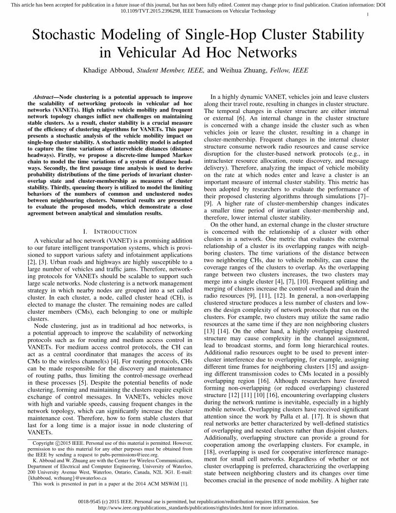
Figure 1. Two neighboring CHs separated by Nc = 4 nodes and Xc =(X0, X1, X2, X3, X4).

possibly-overlapping, single-hop clusters (e.g., [10]). The rangeof each cluster extends one hop on both sides of the CH. At theend of the cluster formation, the vehicles are distributed on thehighway according to a stationary probability distribution of thedistance headways. Let NCM be the number of CMs on oneside of a cluster and let Nc be the number of nodes betweentwo neighbouring CHs. The overlapping range between twoneighbouring clusters is the common distance covered by thetransmission range of both CHs. Define the cluster-overlap statebetween two neighbouring clusters to be i) overlapping, whenthe distance between the two CHs is less than 2R; or ii) non-overlapping, otherwise. In our analysis, the 0th time step refersto the time when the cluster formation has just completed. Weassume that the clusters are initially overlapping and the CHsremain the same over a time interval of interest.

B. Node MobilityThe vehicles move according to the microscopic mobility

model proposed in [20]. In this model, a distance headway,X, changes according to a discrete-time finite-state Markovchain. The Markov chain has Nmax states corresponding to Nmaxranges of a distance headway. Let Xi(m) ∈ si denote the eventthat the ith distance headway is in state si at the mth time step1,where si ∈ [0, Nmax − 1] and i,m ≥ 0. The distance headwaytransits from one state to another according to a tri-diagonalstate-dependent transition matrix, denoted by M . Within a timestep, a distance headway in state j can transit to the next state,the previous state, or remain in the same state with probabilitiespj , qj , or rj , 0 ≤ j ≤ Nmax − 1, respectively, where q0 =pNmax−1 = 0 and rj = 1− pj − qi.

III. EXTERNAL CLUSTER STABILITY

The cluster-overlap state is governed by the the distancebetween two neighboring CHs. As this distance decreases,the CHs approach each other causing the two clusters tooverlap. On the other hand, as the distance between CHsincreases, the CHs move apart from each other causing thetwo clusters to become disjoint. The distance between twoneighboring CHs is equal to the sum of the distance headwaysbetween the two nodes. Label the (Nc + 2) nodes with IDs0, 1, . . . , Nc + 1, where the following CH has ID 0 andthe leading CH has ID (Nc + 1). For notation simplicity,

1The length of the range covered by each state is a constant, denoted by Ls

in meters. The range is chosen such that Ls ≥ τ v where v is the maximumrelative speed between vehicles and τ is the constant time step size. Themobility model parameters are described in details in [20].



3

1OV 1NOV 2NOV

Ω1

Ω2

Ω3

Ω4

Ω5

Ω6

Ω8

Ω7

Ω10

Ω9

2OV

NOVOV

Intertransition between ΩOV

and ΩNOV

Intratransition in ΩOV (ΩNOV)

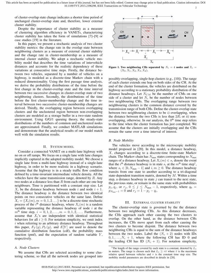
Figure 2. An illustration of a lumped markov chain for N = 2, Nth = 4, Nmax = 3. A line between two lumped states represents a non-zero two-waytransition probability in a single time step between the linked states. There exist non-zero transition probabilities between subsets of ΩOV 1

and ΩNOV 1.

let Xc = (Xi)Nci=0 be the sequence of distance headways

between the two CHs as illustrated in Figure 1, whereXc(m) = (Xi(m))Nc

i=0, and Xc(m) ∈ (s0, s1, . . . , sNc)

≡ Xi(m) ∈ si,∀i ∈ [0, Nc]. Consider initially overlappingclusters, i.e.,

∑Nc

i=0Xi(0) < 2R. Two neighboring CHs remainoverlapping until

∑Nc

i=0Xi (m) ≥ 2R at some time stepm. The sequence of (Nc + 1) independent and identicallydistributed (i.i.d.) distance headways is an (Nc+1)-dimensionalMarkov chain, where each headway, Xi, is a birth and deathMarkov chain as described in Subsection II-B. For clarity, theterm state refers to a state in the original Markov chain, X , theterm super state refers to a state in the (Nc + 1)-dimensionalMarkov chain, and the term lumped state refers to a set ofsuper states (to be discussed later in this section). Additionally,parentheses ( ) are used for a sequence, while curly brackets are used for a set. A super state in the (Nc + 1)-dimensionalMarkov chain is a sequence of size Nc + 1, in which the ithelement represents the state (in the 1-dimensional Markovchain) that the ith distance headway belongs to. That is, asuper state, (s0, s1, . . . , sNc), means that distance headway Xi

is in state si ∈ [0, Nmax − 1]. The sum of (Nc + 1) distanceheadways representing the distance between the two CHs canbe calculated from the (Nc + 1)-dimensional Markov chain.The state space size of the (Nc + 1)-dimensional Markovchain is equal to N (Nc+1)

max , making it subject to the state-spaceexplosion problem when Nc is large. However, since we areinterested in the sum of the (Nc + 1) distance headways, thestate space can be reduced according to the following theorem.

Theorem 1: Let X be a discrete-time, birth-death, irre-ducible Markov chain with Nmax finite states, and let setX = (Xi)

N−1i=0 represent a system of N independent copies

of chain X . The N -dimensional Markov chain that representsthe system, X, is lumpable with respect to the state spacepartition Ω = Ω0,Ω1 . . . ,ΩNL

, such that (s.t.) any two superstates in subset Ωi are permutations of the same set of states∀i ∈ [0, NL − 1], where NL = (Nmax+N−1)!

N !(Nmax−1)! is the state spacesize of the lumped Markov chain.

The proof of Theorem 1 and following corollariesare given in the Appendix. Since a lumped state,Ωi = (s0, s1, . . . , sN−1), 0 ≤ i ≤ NL − 1, contains

all super states that are permutations of the same set ofstates, we can write the lumped state as a set of those statesΩi = s0, s1, . . . , sN−1. Since the (Nc + 1)-dimensionalMarkov chain is irreducible, the lumped Markov chain is alsoirreducible [21]. The stationary distribution of the lumpedMarkov chain can be derived from the stationary distributionof the 1-dimensional Markov chain according to the followingCorollary.

Corollary 1: Consider a system of N independent copies ofa finite, discrete-time, birth-death, irreducible Markov chain,X , with stationary distribution (πi)

Nmax−1i=0 . The stationary

distribution of the lumped Markov chain of Theorem 1, rep-resenting the system, X = (Xi)

N−1i=0 , follows a multi-nomial

distribution with parameters (πi)Nmax−1i=0 .

A. Time to the first change of cluster-overlap stateConsider two overlapping clusters. At any time instant,

the overlapping range between two neighbouring clusters isequal to 2R −

∑Nc

i=0Xi(m), ∀m ≥ 0. Therefore, accordingto Theorem 1, the time variation of the overlapping rangebetween the two clusters can be described by a lumpedMarkov chain with lumped states Ω0,Ω1, . . . ,ΩNL−1 whichrepresents the system, Xc = (Xi)

Nci=0. Furthermore, divide

the lumped states into two sets, ΩOV and ΩNOV . A lumpedstate Ωi = s0, s1, . . . , sNc

belongs to ΩOV and to ΩNOV if∑Nc

i=0 si < 2NR and∑Nc

i=0 si ≥ 2NR, respectively, where NRis the integer number of the states that cover distance headwayswithin R in the distance headway’s 1-dimensional Markovchain. Let the system of the distance headways between thetwo CHs be initially in super state Ic, i.e., Xc(0) ∈ Ic, s.t.Ic ∈ Ωk ∈ ΩOV , 0 ≤ k ≤ NL − 1. Let the time perioduntil the clusters are no longer overlapping be Tov1(Ωk), giventhat the distance headways between them are initially in statesIc ∈ Ωk. Then, this time period is equal to the first passagetime for the system, Xc, to transit from the lumped state Ωk toany lumped state Ωk′ , s.t. Ωk′ ∈ ΩNOV . That is, Tov1(Ωk) =

minm > 0; Xc(m) ∈ (k0, k1, . . . , kNc

),∑Nc

i=0 ki ≥ 2NR |

Xc(0) ∈ Ic

. Let MNcbe the transition probability matrix of

the lumped Markov chain describing Xc. One way to find thefirst passage time is to force the lumped states in ΩNOV to



4

become absorbing, i.e., set the probability of returning to thesame lump state, Ωi, within one time step to one ∀Ωi ∈ ΩNOV .Furthermore, let all the lumped states in ΩNOV be merged intoone single absorbing state and let it be the last (NL − 1)th

state, where NL is the number of states in the new absorbinglumped Markov chain. The transition probability matrix ofthe new absorbing lumped Markov chain, MNc

, is derivedfrom MNc

as follows: MNc(Ωi,Ωj) = MNc

(Ωi,Ωj) ∀i, j, s.t.Ωi,Ωj ∈ ΩOV , MNc

(Ωi,ΩNL−1) =∑jMNc

(Ωi,Ωj) ∀i, j,s.t.Ωi ∈ ΩOV and Ωj ∈ ΩNOV . Let Tov1(Ωk) denote the timeinterval from the instant that the clusters are initially formedtill the first time instant that the cluster-overlap state changes,given that the distance headways are in super state Ic ∈ Ωk.The cdf of Tov1(Ωk) is given by

FTov1(Ωk)(m) = MNc(Ωk,ΩNL−1)

+∑j

Ωj∈ΩOV

MNc(Ωk,Ωj)FTov1(Ωj)(m− 1),

m ≥ 1 (1)

where FTov1(Ωk)(0) = 0. Equation (1) calculates thecdf of Tov1(Ωk) recursively. Since FTov1(Ωk)(m) =∑mn=1 PTov1(Ωk)(m), the first term in (1) corresponds to the

absorption probability within one time step given that thesystem is initially in lumped state Ωk, i.e., FTov1(Ωk)(1) =

MNc(Ωk,ΩNL−1). The second term in (1) corresponds to∑m

n=2 PTov1(Ωk)(m) which is the absorption probability within(m− 1) time steps given that the system transited from Ωk toΩj ∈ ΩOV within one time step.

The size of the state space of the lumped Markov chaincan still be large with an increased number of nodes betweenthe two CHs, since NL = (Nmax+Nc)!

(Nc+1)!(Nmax−1)! . However, thestate space of the absorbing lumped Markov chain, neededto compute the time period until the overlap state changesbetween the two neighboring CHs, is bounded according tothe following Corollary.

Corollary 2: Consider a system of N independent copiesof an irreducible Markov chain according in Theorem 1, andlet the event of interest be that the sum of the states of theN chains be larger than a deterministic threshold Nth. Theabsorbing lumped Markov chain, required to obtain the firstoccurrence time of the event of interest, has a state space thatis bounded by a deterministic function of Nth, when N > Nth.

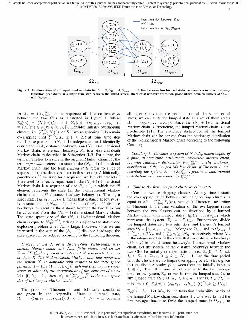
Consider the scalability of analyzing a system of N distanceheadways, XN , to an increased number of distance headways,N . Using the lumped Markov chain, the scalability of analyzingsystem XN is improved for: i) the steady-state analysis -The problem of finding the stationary distribution of a systemof distance headway is of constant computational complexitywith respect to N (according to Corollary 1); and ii) thetransient analysis (i.e, the first passage time analysis) - Thecomputational complexity of the first passage time analysis isdependent on the state space size of the considered Markovchain. According to Corollary 2, the state space size of theabsorbing lumped Markov chain is upper bounded by the totalnumber of integer partitions of all integer that are less than Nthas discussed in Appendix A.3. Figure 3 shows the state spacereduction using the proposed lumped Markov chain.

In this subsection, we focus on the time interval from theinstant that two partially overlapping neighboring clusters are

5 10 15 200

1

2x 10

19

(a)

NN

max

N−Dimensional Markov chain

5 10 15 200

2

4x 10

6

(b)

NL

Lumped Markov chain

5 10 15 200

20

40

NL

N (c)

Absorbing lumped Markov chain

Figure 3. The state space size of a Markov chain representing a systemof N Markov chains (distance headways), XN , with Nmax = 9when the system XN is represented by (a) an N-dimensionalMarkov chain, (b) a lumped Markov chain according to The-orem 1, and (c) an absorbing lumped Markov chain accordingto Corollary 2 with Nth = 8.

formed till the time instant that they no longer overlap. Givenan initial super state of the two neighboring clusters at theend of the cluster formation stage, consider the following: i)a proactive re-clustering procedure in which re-clustering istriggered after a fixed period of time, say ∆t seconds from thecluster formation; and ii) a reactive re-clustering procedure inwhich re-clustering is triggered when the cluster-overlap statechanges. In i), the probability that the overlap state changesbetween the two overlapping neighboring clusters before re-clustering is triggered is equal to FTov1(Ωk)(∆t). In ii), the re-clustering period is equal to Tov1(Ωk) with the cdf calculatedby (1). Up until now, we have considered a pair of neighboringclusters in a specific super state when they are initially formed.In reality, the initial state of a pair of neighboring clusters is arandom variable. For a given Nc, since the distance headwaysare stationary when the clusters are formed, the probability thattwo overlapping neighboring clusters are initially in lumped

state Ωi is given by fi/[ ∑

j,Ωj∈ΩOV

fj

]where fi is given by

(22) in Appendix A.2. Using the law of total probability, thecdf of the time for the first change in overlap state to occurbetween two initially overlapping clusters is given by

FTov1(m) =

∑j

Ωj∈ΩOV

fjFTov1(Ωj)(m)

∑i

Ωi∈ΩOV

fi, m = 1, 2, . . . . (2)



5

B. Time period between successive changes of cluster-overlapstate

In the preceding subsection, we have analysed the timeinterval during which two neighboring clusters remain over-lapping since the clusters are formed. During this time in-terval, the cluster-overlap state remains unchanged. Supposetwo neighboring clusters overlap in cluster formation and theoverlap state changes at time Tov1(< ∆t) and becomes non-overlapping. The cluster-overlap state may change again beforere-clustering is triggered. As a result, the time period betweentwo consecutive changes of cluster-overlap state equals i) thecluster-overlapping time period when the overlap state changesfrom overlapping to non-overlapping, plus ii) the cluster-non-overlapping time period when the overlap state changes fromnon-overlapping to overlapping. During a cluster-overlappingor cluster non-overlapping time periods, the cluster-overlapstate remains unchanged indicating how long the cluster re-mains externally stable.

1) Cluster-overlapping time period:The second cluster-overlapping time period may not be equalto Tov1, since the initial state may not be the same as thatwhen the clusters are initially formed. We refer to this periodas cluster overlapping period, denoted by Tov .

To derive the distribution of Tov , the same approach usedto find the distribution of Tov1 can be used. Notice that theabsorbing lumped Markov chain is the same as that usedto calculate the distribution of Tov1. The only difference isthe distribution of the initial state, Ic. One way to find thedistribution of Ic at the time when the second overlappingstate occurs is as follows:

• Make the lumped states in set ΩNOV absorbing, withoutcombining them into one absorbing state. The corre-sponding transition probability matrix, M ′′Nc , is equalto MNc with M ′′Nc(Ωj ,Ωi) = 0 and M ′′Nc(Ωj ,Ωj) =1∀i, j, s.t. Ωj ∈ ΩNOV ;

• Calculate the absorbing probability ψj for each absorbinglumped state Ωj ∈ ΩNOV by

ψj =∑i

Ωi∈ΩOV

fi∑k

Ωk∈ΩOV

fklimm→∞

M ′′(m)Nc

(Ωi,Ωj) (3)

where M ′′(m)Nc

(Ωi,Ωj) denotes the (Ωi,Ωj)th entry of the mth

power of matrix M ′′Nc;

• Form another absorbing Markov chain by making thelumped states in set ΩOV absorbing, without combiningthem into one absorbing state. The corresponding tran-sition probability matrix, M ′Nc , is equal to MNc withM ′Nc(Ωi,Ωj) = 0 and M ′Nc(Ωi,Ωi) = 1 ∀i, j, s.t.Ωi ∈ ΩOV ;

• Calculate the absorbing probability φi for each absorbinglumped state Ωi ∈ ΩOV by

φi =∑j

Ωj∈ΩNOV

ψj limm→∞

M ′(m)Nc

(Ωj ,Ωi). (4)

The probability that the distance headways between the twoneighboring clusters are in state Ωi ∈ ΩOV at the time whenthe second overlapping state occurs is equal to φi. Therefore,the cdf of the cluster-overlapping period is given by

FTov(m) =

∑i

Ωi∈ΩOV

φiFTov1(Ωi)(m),m = 1, 2, . . . (5)

where FTov1(Ωi)(m) is given by (1). However, using this ap-proach, we lose the advantage of having a single absorbing stateand, therefore, a bounded state space (according to Corollary 2).We propose to approximate the distribution of the system initialstate at the time when the second overlapping state occurs, φi,as follows

φi ≈fiMNc

(Ωi,ΩNL−1)∑i

Ωi∈ΩOV

fiMNc(Ωi,ΩNL−1). (6)

The approximated φi for lumped state Ωi(∈ ΩOV ) is equalto its stationary probability weighted with the absorptionprobability within one time step. Notice that this weighteliminates all the lumped states Ωi ∈ ΩOV that are notdirectly accessible from states in ΩNOV . Figure 2 illustratesan example for a lumped Markov chain, where the directlyaccessible lumped states are those connected by solid lines,i.e. ΩOV 1 and ΩNOV 1. When the overlapping state oftwo neighboring clusters changes from non-overlapping tooverlapping, the only possible states to be reached first arethose in ΩOV 1.

2) Cluster-non-overlapping time period:Consider two initially overlapping clusters, the cluster statecan change to become non-overlapping and again to becomeoverlapping. The time period between two consecutive changesof cluster-overlap state equals the cluster-non-overlapping timeperiod when the state changes from non-overlapping to over-lapping. Neighboring CHs may move apart from each other andthe clusters become disjoint. This may result in disruption tointercluster and/or intracluster communications and/or seizureof the cluster membership status from edge CMs. This producesunclustered nodes that may create their own cluster whichcan trigger re-clustering and increase the clustering cost. LetTnov denote the cluster non-overlapping time period. The sameprocedure used to calculate the cdf of Tov can be used to derivethe cdf of Tnov , which is given by

FTnov(m) =

∑j

Ωj∈ΩNOV

ψjFTnov1(Ωj)(m),m = 1, 2, . . . (7)

where FTnov1(Ωj)(m) = M ′Nc(Ωj ,ΩN ′L−1) +

∑k

Ωk∈ΩNOV

[M ′Nc

(Ωj ,Ωk)FTnov1(Ωk)(m − 1)],m ≥ 1, ψj ≈

fjM ′Nc (Ωj ,ΩN′L−1)∑

jΩj∈ΩNOV

fjM ′Nc (Ωj ,ΩN′L−1), and M ′Nc

is the probability

transition matrix that corresponds to the lumped Markovchain with all states in ΩOV combined into one absorbingstate. That is, M ′Nc

is derived from MNcas follows:

M ′Nc(Ωj ,Ωi) = MNc(Ωj ,Ωi) ∀i, j, s.t. Ωj ,Ωi ∈ ΩNOV ,

M ′Nc(Ωj ,ΩN ′L−1) =

∑jMNc

(Ωj ,Ωi) ∀i, j, s.t.Ωj ∈ ΩNOVand Ωi ∈ ΩOV . The average cluster-non-overlapping timeperiod is given by [22]

E[Tnov] = Ψ(I − M ′Nc

)−1

M1 (8)

where Ψ is a row vector of size N ′L in which the jth elementequals ψj , I is the identity matrix of size equal to that of N ′L,and M1 is a column vector of ones with size N ′L. The secondmoment of the cluster-non-overlapping time period is given by2

2The first and the second moments of the cluster-overlapping period can becalculated similarly by adjusting (8)-(9) to correspond to the absorbing lumpedMarkov chain with transition matrix MNc .



6

R

CH

R

loe

lie

roe rie

CM

Figure 4. Illustration of the events that cause changes in cluster-membership.

[22]

E[T 2nov] = 2ΨM ′Nc

(I − M ′Nc

)−2

M1 + E[Tnov]. (9)

IV. INTERNAL CLUSTER STABILITY

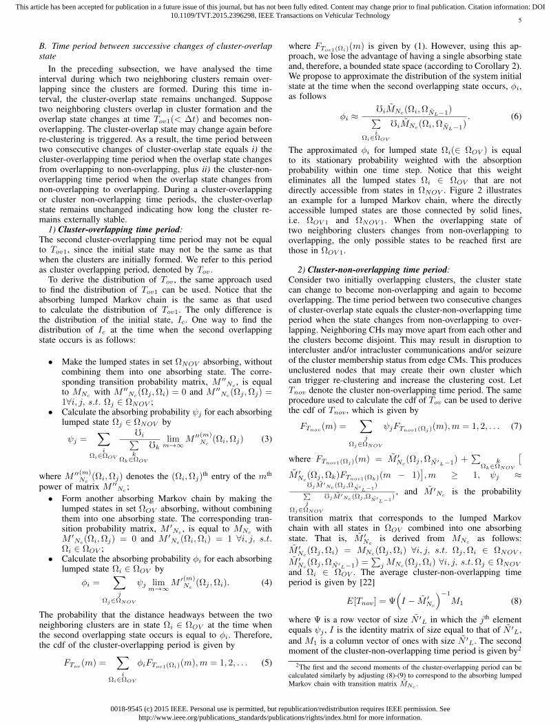
Due to relative vehicle mobility, two events result inchanges to the cluster-membership: i) a vehicle leaving thecluster, and ii) a vehicle entering the cluster. Let eor and eoldenote the events that a vehicle leaves the cluster from theright side and the left side of the CH, respectively. Let eirand eil denote the events that a vehicle enters the clusterfrom the right side and the left side of the CH, respectively.Figure 4 illustrates these events. Consider the time for thefirst change in cluster-membership to occur after clusterformation, and denote this time by TCM1. This time isequivalent to the first occurrence times of one of the fourevents, i.e., TCM1 = T (eor ∪ eir ∪ eol ∪ eil), where T (e)denotes the first occurrence time of event e. Furthermore, letTCM1r = T (eor ∪ eir ) and TCM1l

= T (eol ∪ eil) be the firstoccurrence time of the first change in cluster-membership (aftercluster formation) due to a vehicle leaving and entering thecluster from the right and the left side of the CH, respectively.Therefore, TCM1 = min TCM1r

, TCM1l. Since TCM1r

andTCM1l

are independent, the cdf of the time for the first changein cluster-membership to occur after cluster formation is givenby FTCM1

(m) = 1 − (1 − FTCM1r(m))(1 − FTCM1l

(m)).Notice that TCM1r and TCM1l

are i.i.d.. Therefore, we focuson calculating only one of them, say TCM1r .

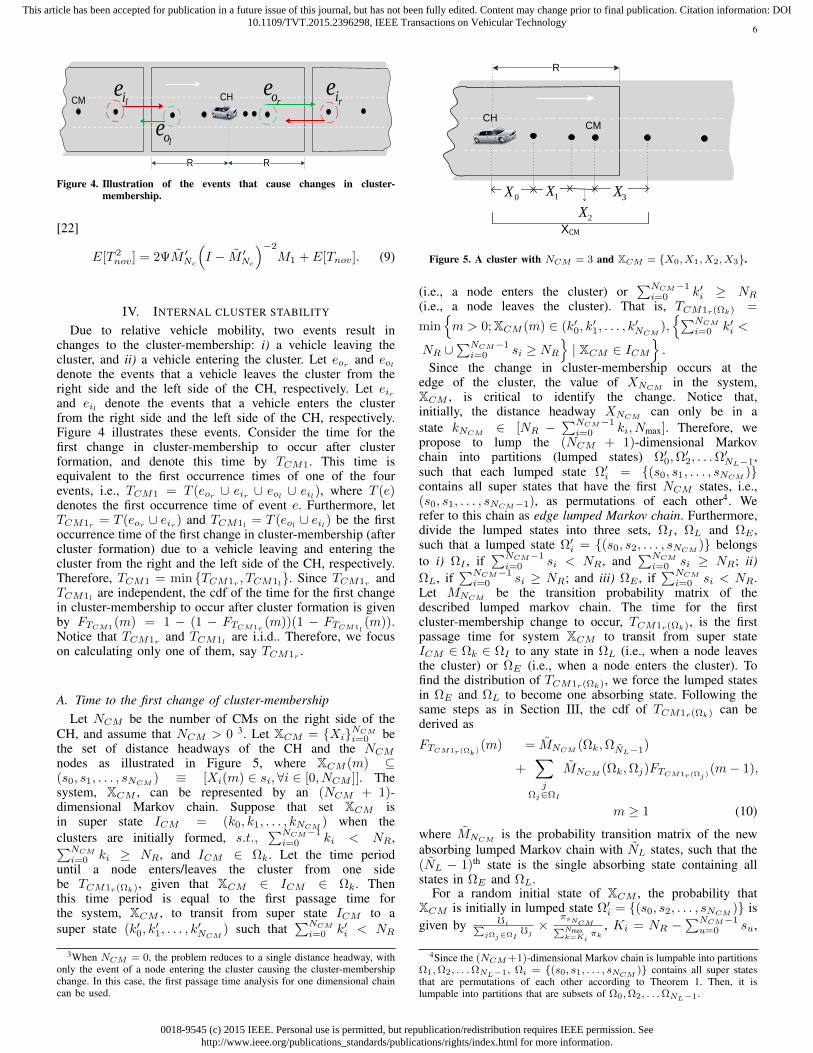
A. Time to the first change of cluster-membershipLet NCM be the number of CMs on the right side of the

CH, and assume that NCM > 0 3. Let XCM = XiNCMi=0 be

the set of distance headways of the CH and the NCMnodes as illustrated in Figure 5, where XCM (m) ⊆(s0, s1, . . . , sNCM

) ≡ [Xi(m) ∈ si,∀i ∈ [0, NCM ]]. Thesystem, XCM , can be represented by an (NCM + 1)-dimensional Markov chain. Suppose that set XCM isin super state ICM = (k0, k1, . . . , kNCM

) when theclusters are initially formed, s.t.,

∑NCM−1i=0 ki < NR,∑NCM

i=0 ki ≥ NR, and ICM ∈ Ωk. Let the time perioduntil a node enters/leaves the cluster from one sidebe TCM1r(Ωk), given that XCM ∈ ICM ∈ Ωk. Thenthis time period is equal to the first passage time forthe system, XCM , to transit from super state ICM to asuper state (k′0, k

′1, . . . , k

′NCM

) such that∑NCM

i=0 k′i < NR

3When NCM = 0, the problem reduces to a single distance headway, withonly the event of a node entering the cluster causing the cluster-membershipchange. In this case, the first passage time analysis for one dimensional chaincan be used.

CH

R

CM

0X

XCM

1X

2X3X

Figure 5. A cluster with NCM = 3 and XCM = X0, X1, X2, X3.

(i.e., a node enters the cluster) or∑NCM−1i=0 k′i ≥ NR

(i.e., a node leaves the cluster). That is, TCM1r(Ωk) =

minm > 0;XCM (m) ∈ (k′0, k

′1, . . . , k

′NCM

),∑NCM

i=0 k′i <

NR ∪∑NCM−1i=0 si ≥ NR

| XCM ∈ ICM

.

Since the change in cluster-membership occurs at theedge of the cluster, the value of XNCM

in the system,XCM , is critical to identify the change. Notice that,initially, the distance headway XNCM

can only be in astate kNCM

∈ [NR −∑NCM−1i=0 ki, Nmax]. Therefore, we

propose to lump the (NCM + 1)-dimensional Markovchain into partitions (lumped states) Ω′0,Ω

′2, . . .Ω

′NL−1,

such that each lumped state Ω′i = (s0, s1, . . . , sNCM)

contains all super states that have the first NCM states, i.e.,(s0, s1, . . . , sNCM−1), as permutations of each other4. Werefer to this chain as edge lumped Markov chain. Furthermore,divide the lumped states into three sets, ΩI , ΩL and ΩE ,such that a lumped state Ω′i = (s0, s2, . . . , sNCM

) belongsto i) ΩI , if

∑NCM−1i=0 si < NR, and

∑NCM

i=0 si ≥ NR; ii)ΩL, if

∑NCM−1i=0 si ≥ NR; and iii) ΩE , if

∑NCM

i=0 si < NR.Let MNCM

be the transition probability matrix of thedescribed lumped markov chain. The time for the firstcluster-membership change to occur, TCM1r(Ωk), is the firstpassage time for system XCM to transit from super stateICM ∈ Ωk ∈ ΩI to any state in ΩL (i.e., when a node leavesthe cluster) or ΩE (i.e., when a node enters the cluster). Tofind the distribution of TCM1r(Ωk), we force the lumped statesin ΩE and ΩL to become one absorbing state. Following thesame steps as in Section III, the cdf of TCM1r(Ωk) can bederived as

FTCM1r(Ωk)(m) = MNCM

(Ωk,ΩNL−1)

+∑j

Ωj∈ΩI

MNCM(Ωk,Ωj)FTCM1r(Ωj)

(m− 1),

m ≥ 1 (10)

where MNCMis the probability transition matrix of the new

absorbing lumped Markov chain with NL states, such that the(NL − 1)th state is the single absorbing state containing allstates in ΩE and ΩL.

For a random initial state of XCM , the probability thatXCM is initially in lumped state Ω′i = (s0, s2, . . . , sNCM

) isgiven by fi∑

jΩj∈ΩIfj×

πsNCM∑Nmaxk=Ki

πk, Ki = NR −

∑NCM−1u=0 su,

4Since the (NCM +1)-dimensional Markov chain is lumpable into partitionsΩ1,Ω2, . . .ΩNL−1, Ωi = (s0, s1, . . . , sNCM

) contains all super statesthat are permutations of each other according to Theorem 1. Then, it islumpable into partitions that are subsets of Ω0,Ω2, . . .ΩNL−1.



7

where fi is the stationary distribution of lumped state Ωi =(s0, s2, . . . , sNCM−1) of the NCM -dimensional Markovchain lumped according to Theorem 1. Hence, the cdf of thetime interval between the time instant when the cluster isinitially formed till the first cluster-membership change is givenby

FTCM1r(m) =

1∑j

Ω′j∈ΩI

fj

∑i

Ω′i∈ΩI

π(i,sNCM)fiFTCM1r(Ω′

i)(m)∑Nmax

k=Kiπk

(11)where (i, sNCM

) is the state index of the distance headway ofthe N th

CM CM in the ith lumped state.

B. Time period between successive changes of cluster-membership

In the previous subsection, we have analysed the time inter-val from initial cluster formation to the first cluster-membershipchange. In order to have a better measure of internal clusterstability, we analyse the time interval between two successivecluster-membership changes in this subsection. Let TCM de-note the time interval between two consecutive membershipchanges of a cluster. Notice that the cluster-membership changerate, i.e. the rate at which nodes enter or leave the cluster, isthe reciprocal of TCM . We focus on one side of the cluster inthis subsection, since a similar derivation for the other side canbe done.

To derive the distribution of TCM , the first step is to findthe distribution of ICM at the time when the first cluster-membership change occurs. In order to do this, first we makethe lumped states in sets ΩE and ΩL of the lumped Markovchain absorbing, without combining them into one state. Theresult is an absorbing markov chain and let M ′CM be itsprobability transition matrix. Then the probability of absorptionin lumped state Ωe ∈ ΩE and the probability of absorption inlumped state Ωl ∈ ΩL are given respectively by

ψEe=

1∑j

Ω′j∈ΩI

fj

∑i

Ω′i∈ΩI

π(i,sNCM )fi∑Nmax

k=Kiπk

limm→∞

M ′(m)NCM

(Ωi,Ωe)

and

ψLl=

1∑j

Ω′j∈ΩI

fj

∑i

Ω′i∈ΩI

π(i,sNCM )fi∑Nmax

k=Kiπk

limm→∞

M ′(m)NCM

(Ωi,Ωl)

where M ′(m)NCM

(Ωi,ΩE) denotes the (Ωi,ΩE)th entry of themth power of matrix M ′NCM

. Note that∑ψEee

Ωe∈ΩE

and∑ψLl

lΩl∈ΩL

are the probabilities that the first cluster-membership changeoccurs due to a vehicle entering the cluster and leaving thecluster, respectively. When calculating the time interval be-tween successive cluster-membership changes, the examinedsystem changes. Let XCME

and XCMLbe the systems of

distance headways of the CH and the nodes on one side ofthe cluster when the first cluster-membership change occursdue to a node entering the cluster and a node leaving thecluster, respectively. For example, if system XCM is absorbedin lumped state Ωi = (s0, s1, . . . sNCM

), then the initiallumped state for system XCML

is (s0, s1, . . . sNCM−1) ifΩi ∈ ΩL and the initial lumped state for system XCME

is(s0, s1, . . . sNCM

, sNCM+1) if Ωi ∈ ΩE , where sNCM+1 ∈

-1(seconds)

1

Figure 6. Illustration of the alternating renewal process between overlap-ping and non-overlapping time periods.

[NR−∑NCM

i=0 si, Nmax]. Let Ω′e be the lumped state for systemXCME

corresponding to lumped state Ωe for XCM , and let Ω′lbe the lumped state for system XCML

corresponding to lumpedstate Ωl for XCM . Additionally, let ψE′e equal ψEe weightedby the stationary distribution (21) to account for the addeddistance headway in the system, XCME

. The cdf of the timeinterval between two successive cluster-membership changes isapproximated by

FTCM(m) =

∑e

Ωe∈ΩE

ψE′eFTCM1e(Ω′e)(m)

+∑l

Ωl∈ΩL

ψLlFTCM1l(Ω

′l)(m). (12)

V. NUMBERS OF COMMON CMS AND UNCLUSTEREDNODES BETWEEN CLUSTERS

In Section III, the time for the first change in cluster-overlap state along with the cluster-overlapping and cluster-non-overlapping time periods are studied. Despite the impor-tance of the change in overlap-state as a measure of externalcluster stability, it is a binary metric. A quantitative metric thatdescribes in detail the level of external stability is desired. Onequantitative measure is the number of nodes located betweenthe clusters. That is, the number of nodes shared betweenoverlapping clusters and the number of nodes left unclus-tered between disjoint clusters. The number of common nodesbetween neighboring clusters is an indicator of the level ofintercluster communication interference that can occur duringthe overlapping period. On the other hand, during the non-overlapping period, the number of unclustered nodes betweendisjoint clusters is an indicator of the portion of network nodesthat are left unserved by the clustered structure.

Given initially overlapping neighboring clusters, vehicles canenter and leave the overlapping/unclustered region. Addition-ally, the cluster-overlap state may change over time. Therefore,in this section we investigate the system of two neighboringclusters in terms the change of the numbers of common CMsand unclustered nodes between the two clusters along with thechange in the cluster-overlap state. Since the system of distanceheadways between the neighboring clusters, Xc, constructs afinite irreducible lumped Markov chain, there exists an infinitesequence of cluster-overlapping and cluster-non-overlappingtime periods [22]. Therefore, the overlap state between clustersfluctuates between overlapping and non-overlapping scenarios.

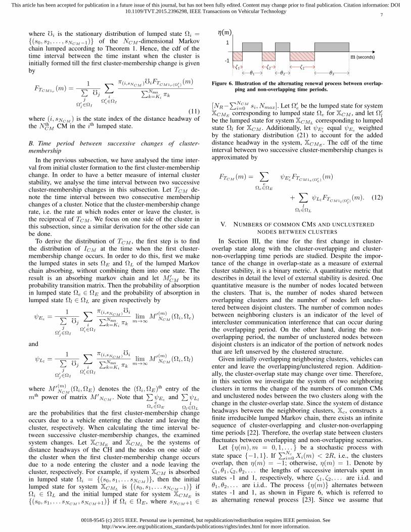
Let η(m),m = 0, 1, . . . be a stochastic process withstate space −1, 1. If

∑Nc

i=0Xi(m) < 2R, i.e., the clustersoverlap, then η(m) = −1; otherwise, η(m) = 1. Denote byζ1, θ1, ζ2, θ2, . . . the lengths of successive intervals spent instates -1 and 1, respectively, where ζ1, ζ2, . . . are i.i.d. andθ1, θ2, . . . are i.i.d.. The process η(m) alternates betweenstates -1 and 1, as shown in Figure 6, which is referred toas alternating renewal process [23]. Since we assume that



8

CH

R

CH

R

CM

unclustered node

Unclusteredregion

CH

R

CMCH

R

Overlapping region

(b)

(a)

common CM

Figure 7. Illustration of the events that cause a vehicle to (a) enter theoverlapping region and (b) leave the unclustered region betweenneighboring clusters.

the clusters are initially overlapping, then η(0) = −1 andζk = T kov , and θk = T knov , i.e., kth cluster-overlapping periodand the kth cluster-non-overlapping period, respectively. Weassume that the T kov’s are i.i.d. with cdf (5) and the T knov’stime periods are i.i.d. with cdf (7) and they are independent ofone another5. The kth cycle is composed of ζk and θk.

A. Node interarrival time during an overlapping/non-overlapping period

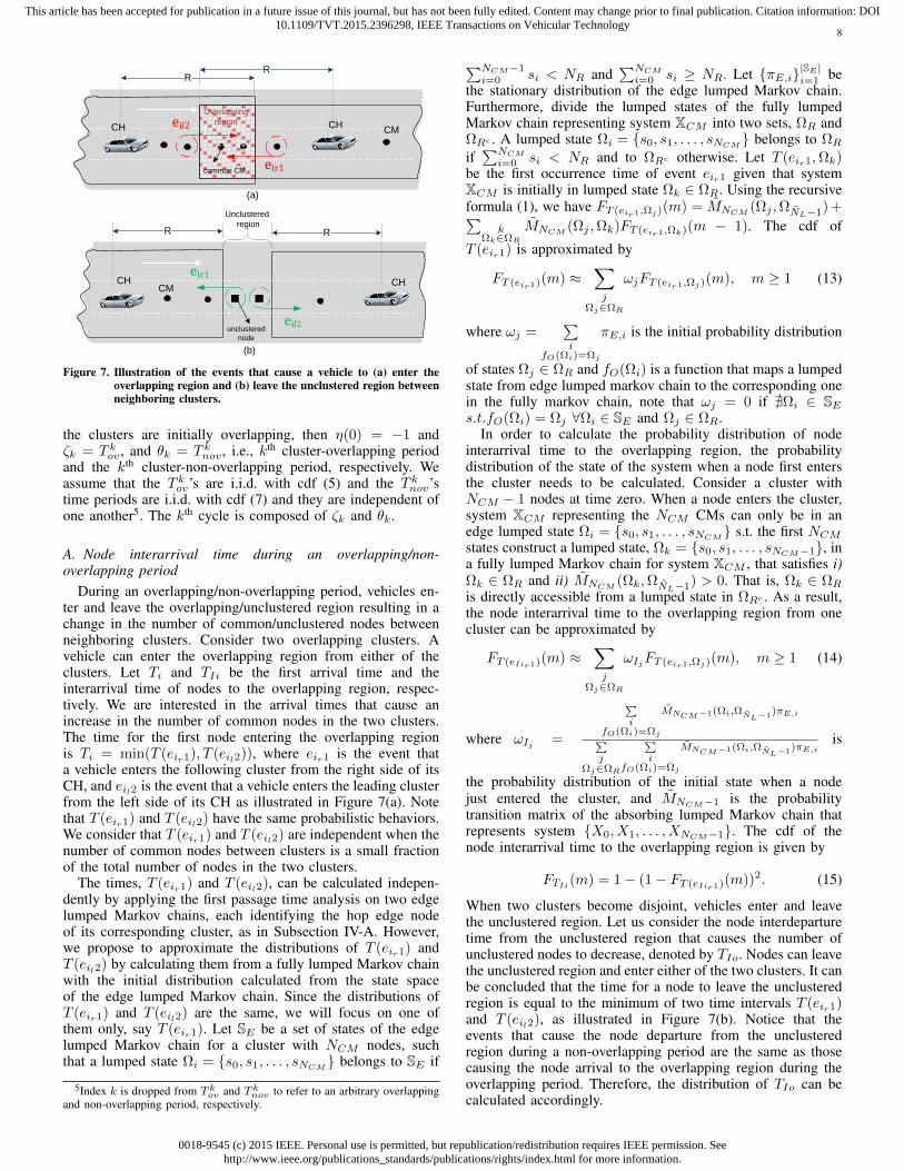
During an overlapping/non-overlapping period, vehicles en-ter and leave the overlapping/unclustered region resulting in achange in the number of common/unclustered nodes betweenneighboring clusters. Consider two overlapping clusters. Avehicle can enter the overlapping region from either of theclusters. Let Ti and TIi be the first arrival time and theinterarrival time of nodes to the overlapping region, respec-tively. We are interested in the arrival times that cause anincrease in the number of common nodes in the two clusters.The time for the first node entering the overlapping regionis Ti = min(T (eir1), T (eil2)), where eir1 is the event thata vehicle enters the following cluster from the right side of itsCH, and eil2 is the event that a vehicle enters the leading clusterfrom the left side of its CH as illustrated in Figure 7(a). Notethat T (eir1) and T (eil2) have the same probabilistic behaviors.We consider that T (eir1) and T (eil2) are independent when thenumber of common nodes between clusters is a small fractionof the total number of nodes in the two clusters.

The times, T (eir1) and T (eil2), can be calculated indepen-dently by applying the first passage time analysis on two edgelumped Markov chains, each identifying the hop edge nodeof its corresponding cluster, as in Subsection IV-A. However,we propose to approximate the distributions of T (eir1) andT (eil2) by calculating them from a fully lumped Markov chainwith the initial distribution calculated from the state spaceof the edge lumped Markov chain. Since the distributions ofT (eir1) and T (eil2) are the same, we will focus on one ofthem only, say T (eir1). Let SE be a set of states of the edgelumped Markov chain for a cluster with NCM nodes, suchthat a lumped state Ωi = s0, s1, . . . , sNCM

belongs to SE if

5Index k is dropped from Tkov and Tk

nov to refer to an arbitrary overlappingand non-overlapping period, respectively.

∑NCM−1i=0 si < NR and

∑NCM

i=0 si ≥ NR. Let πE,i|SE |i=1 bethe stationary distribution of the edge lumped Markov chain.Furthermore, divide the lumped states of the fully lumpedMarkov chain representing system XCM into two sets, ΩR andΩRc . A lumped state Ωi = s0, s1, . . . , sNCM

belongs to ΩRif∑NCM

i=0 si < NR and to ΩRc otherwise. Let T (eir1,Ωk)be the first occurrence time of event eir1 given that systemXCM is initially in lumped state Ωk ∈ ΩR. Using the recursiveformula (1), we have FT (eir1,Ωj)(m) = MNCM

(Ωj ,ΩNL−1) +∑k

Ωk∈ΩR

MNCM(Ωj ,Ωk)FT (eir1,Ωk)(m − 1). The cdf of

T (eir1) is approximated by

FT (eir1)(m) ≈∑j

Ωj∈ΩR

ωjFT (eir1,Ωj)(m), m ≥ 1 (13)

where ωj =∑i

fO(Ωi)=Ωj

πE,i is the initial probability distribution

of states Ωj ∈ ΩR and fO(Ωi) is a function that maps a lumpedstate from edge lumped markov chain to the corresponding onein the fully markov chain, note that ωj = 0 if @Ωi ∈ SEs.t.fO(Ωi) = Ωj ∀Ωi ∈ SE and Ωj ∈ ΩR.

In order to calculate the probability distribution of nodeinterarrival time to the overlapping region, the probabilitydistribution of the state of the system when a node first entersthe cluster needs to be calculated. Consider a cluster withNCM − 1 nodes at time zero. When a node enters the cluster,system XCM representing the NCM CMs can only be in anedge lumped state Ωi = s0, s1, . . . , sNCM

s.t. the first NCMstates construct a lumped state, Ωk = s0, s1, . . . , sNCM−1, ina fully lumped Markov chain for system XCM , that satisfies i)Ωk ∈ ΩR and ii) MNCM

(Ωk,ΩNL−1) > 0. That is, Ωk ∈ ΩRis directly accessible from a lumped state in ΩRc . As a result,the node interarrival time to the overlapping region from onecluster can be approximated by

FT (eIir1)(m) ≈∑j

Ωj∈ΩR

ωIjFT (eir1,Ωj)(m), m ≥ 1 (14)

where ωIj =

∑i

fO(Ωi)=Ωj

MNCM−1(Ωi,ΩNL−1)πE,i

∑j

Ωj∈ΩR

∑i

fO(Ωi)=Ωj

MNCM−1(Ωi,ΩNL−1)πE,iis

the probability distribution of the initial state when a nodejust entered the cluster, and MNCM−1 is the probabilitytransition matrix of the absorbing lumped Markov chain thatrepresents system X0, X1, . . . , XNCM−1. The cdf of thenode interarrival time to the overlapping region is given by

FTIi(m) = 1− (1− FT (eIir1)(m))2. (15)

When two clusters become disjoint, vehicles enter and leavethe unclustered region. Let us consider the node interdeparturetime from the unclustered region that causes the number ofunclustered nodes to decrease, denoted by TIo. Nodes can leavethe unclustered region and enter either of the two clusters. It canbe concluded that the time for a node to leave the unclusteredregion is equal to the minimum of two time intervals T (eir1)and T (eil2), as illustrated in Figure 7(b). Notice that theevents that cause the node departure from the unclusteredregion during a non-overlapping period are the same as thosecausing the node arrival to the overlapping region during theoverlapping period. Therefore, the distribution of TIo can becalculated accordingly.



9

B. Steady-state distributions of the numbers of common CMsand unclustered nodes

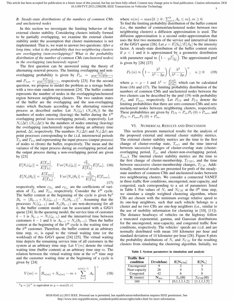
In this section we investigate the limiting behavior of theexternal cluster stability. Considering clusters initially formedto be partially overlapping, we examine the external clusterstability under the assumption that cluster maintenance is notimplemented. That is, we want to answer two questions: After along time, what is the probability that two neighboring clustersare overlapping (non-overlapping)? What is the probabilitydistribution of the number of common CMs (unclustered nodes)in the overlapping (unclustered) region?

The first question can be answered using the theory ofalternating renewal process. The limiting overlapping and non-overlapping probability is given by Pov = E[Tov ]

E[Tov ]+E[Tnov ]

and Pnov = E[Tnov ]E[Tov ]+E[Tnov ] , respectively [23]. For the second

question, we propose to model the problem as a storage bufferwith a two-state random environment [24]. The buffer contentrepresents the number of nodes in the overlapping/unclusteredregion between neighboring clusters. The two random statesof the buffer are the overlapping and the non-overlappingstates which fluctuate according to the alternating renewalprocess as described earlier. Let Ni(ζk) (No(θk)) be thenumbers of nodes entering (leaving) the buffer during the kth

overlapping period (non-overlapping period), respectively. LetNi(∆t) (No(∆t)) be the numbers of nodes entering (leaving)the overlapping (unclustered) region during an arbitrary timeperiod, ∆t, respectively. The numbers Ni(∆t) and No(∆t) arepoint processes corresponding to the i.i.d. interrenewal periodsTIi and TIo, and representing the input process (output process)of nodes to (from) the buffer, respectively. The mean and thevariance of the input process during an overlapping period andthe output process during a non-overlapping period are givenby [23]

E[Ni(ζk)] =E[Tov]

E[TIi], V ar[Ni(ζk)] =

c2TIi

E[TIi]E[Tov], (16)

E[No(θk)] =E[Tnov]

E[TIo], V ar[No(θk)] =

c2TIo

E[TIo]E[Tnov],

(17)respectively, where cTIi

and cTIoare the coefficients of vari-

ation of TIi and TIo, respectively. Consider the kth cycle.The buffer content at the beginning of the cycle is given by6

Bk = [Bk−1 +Ni(ζk−1)−No(θk−1)]+. Assuming that the

processes Ni(ζk−1) and No(θk−1) are non-decreasing for allk, the buffer content model can be associated with a G/G/1queue [24]. In the queueing model, the service time of customerk − 1 is Sk−1 = Ni(ζk−1) and the interarrival time betweencustomers k − 1 and k is Ak−1 = No(θk−1). Then the buffercontent at the beginning of the kth cycle is the waiting time ofthe kth customer. Therefore, the buffer content at an arbitrarytime step, m, is equal to the virtual waiting time (or theworkload) of this G/G/1 queue [24] [25]. The virtual waitingtime depicts the remaining service time of all customers in thesystem at an arbitrary time step. Let V (m) denote the virtualwaiting time (buffer content) at an arbitrary time step m. Therelation between the virtual waiting time at the mth time stepand the customer waiting time at the beginning of a cycle isgiven by [24]

V (m) =

Bn(m) + Sn(m) −m+

n(m)−1∑k=1

Ak

+

(18)

6y = [x]+ is equivalent to y = max(0, x)

where n(m) = maxk ≥ 0 :∑ki=1Ak ≤ m,m ≥ 0.

To find the limiting probability distribution of the buffer content(i.e., the number of common/unclustered nodes between twoneighboring clusters) a diffusion approximation is used. Thediffusion approximation is a second order-approximation thatuses the first two moments of the service and interarrival timesof the G/G/1 queue [26]. Let ρ = E[Sk]/E[Ak] be the intensityfactor. A steady-state distribution of the buffer content existsif ρ < 1 and it is approximated by a geometric distributionwith parameter equal to

(1− λ2

λ2−2µ

). The approximated pmf

is given by [26] [27]

PV (n) ≈(

1− λ2

λ2 − 2µ

)(λ2

λ2 − 2µ

)n, n ≥ 0 (19)

where µ = ρ − 1 and λ2 =E[S2

k]E[Ak] which can be calculated

from (16) and (17). The limiting probability distribution of thenumbers of common CMs and unclustered nodes between thetwo clusters can be described by the pmf (19) with probabilityPov and Pnov , respectively. Let PC0 and PU0 denote thelimiting probabilities that there are zero common CMs and zerounclustered nodes between neighboring clusters, respectively.These probabilities are given by PC0 = PovPV (0)+Pnov , andPU0 = PnovPV (0) + Pov .

VI. NUMERICAL RESULTS AND DISCUSSION

This section presents numerical results for the analysis ofthe proposed external and internal cluster stability metrics.The external cluster stability metrics are the time to the firstchange of cluster-overlap state, Tov1 and the time intervalbetween successive changes of cluster-overlap state (cluster-overlapping period, Tov and cluster-non-overlapping period,Tnov). The internal cluster stability metrics are the time tothe first change of cluster-membership, TCM1, and the timebetween successive cluster-membership changes, TCM . Addi-tionally, numerical results are presented for pmfs of the steady-state numbers of common CMs and unclustered nodes betweentwo neighbouring clusters. We consider a connected VANETin three traffic flow conditions, uncongested, near-capacity, andcongested, each corresponding to a set of parameters listedin Table I. For values of Nc and NCM at the 0th time step,we simulate a simple weighted clustering algorithm, whereCHs are chosen with the minimum average relative speed toits one-hop neighbors, such that each vehicle belongs to acluster and no two CHs are one-hop neighbors (i.e., similar tothe use of mobility information for clustering in [10], [11]).The distance headways of vehicles on the highway followa truncated exponential, gamma, and Gaussian distributionsfor the uncongested, near-capacity, and congested traffic flowconditions, respectively. The vehicles’ speeds are i.i.d. and arenormally distributed with mean 100 kilometer per hour andstandard deviation of 10 kilometer per hour [28]. Figure 8 plotsthe probability distributions of Nc and NCM for the resultingclusters from simulating the clustering algorithm. Initially, we

Table I. System parameters in simulation and analysis

Traffic flowcondition D(veh/km) E[NCM] E[Nc]

Uncongested 9 2 3Near-capacity 26 4 5

Congested 42 6 8R (meter) Nmax Xc(0) XCM(0)

160 9 0,1,1,1,1,2 1,1,1,1,5



10

Figure 8. The pmfs of (a) the number of nodes between two neighboringCHs, Nc and (b) the number of nodes in a cluster NCM ,calculated from simulating a simple weighted clustering ofvehicles.

0 50 100 150 200 2500

0.005

0.01

0.015

0.02

0.025

0.03

0.035

0.04

i

φ i

SimulationsTheoretical approximationTheoretical exact

Figure 9. The pmf, φi = P (Ic ∈ Ωi), of system Xc being in lumped stateΩi ∈ ΩOV at the instant when the second overlapping clusterstate occurs.

set Nc to its average value from the cluster formation results.For D = 42 vehicles per kilometer (veh/km), we set Ic andICM to the states with highest probability of occurrence at thecluster formation stage. The Markov-chain distance headwaymodel has the following parameters: Nmax = 9, each statecovers 20 meters range of distance headways, the time stepis equal to 2 seconds, and the transition probabilities are tunedaccording to the results in [20]. Based on these parameters, wegenerate time series of distance headway data according to themicroscopic mobility model, using MATLAB. Each simulationconsists of 20,000 iterations.

Figure 9 compares the distribution of the state of systemXc, when the second overlapping state occurs, calculated usingthe exact derivation (4) and the proposed approximation (6).The values on the x-axis represent arbitrary IDs given to thelumped states Ωi ∈ ΩOV . The results from the proposedapproximation shows close agreement with the exact and thesimulation results. Figure 10 plots the pmf of the time interval

Figure 10. The pmfs of (a) the time to the first change in cluster-overlapstate, Tov1(Ωk), for Ic = 0, 1, 1, 1, 1, 2 ∈ Ωk when theclusters are initially formed; (b) the time to the first changein cluster-overlap state Tov1; and (c) the cluster-overlappingtime period, Tov , when D = 26 veh/km.

for the first change in cluster overlapping state, for (a) a giveninitial state of Xc and (b) when averaging over random initialstates, respectively. The theoretical results for the pmfs of thecluster-overlapping period are calculated from the cdf in (5).The calculated pmf of Tov in Figure 10(c) is based on theapproximation given in Figure 9. The distribution of Tov1(Ωk)changes with Ic belonging to different lumped states Ωk. Thedistribution of Tov1 describes the average time before the firstcluster-overlap change for a randomly picked cluster in thenetwork. When clusters overlap, the cluster-overlapping periodis equal to the time period between two successive cluster-ovelap state changes (i.e., the time period of invariant cluster-overlap state). Note that the average time for the first changeof cluster-overlap state is larger than the average time periodbetween successive changes of cluster-overlap state. When thesecond overlapping state occurs between neighouring clusters,the clusters state is closer to non-overlapping than that when theclusters are initially formed, on average. That is, the clustersstate can only be in the accessible lumped states (ΩOV 1 inFigure 2).

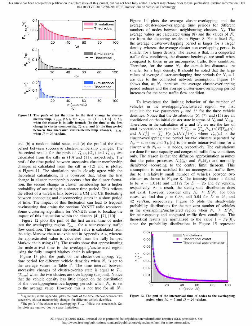
Figure 11 plots the pmf of the time period from the clusterformation till the time step that a first change in cluster-membership occurs for (a) a given initial state ICM ∈ Ωk



11

Figure 11. The pmfs of (a) the time to the first change in cluster-membership, TCM1(Ωk), for ICM = 1, 1, 1, 1, 5 ∈ Ωk

when the cluster is initially formed; (b) the time to the firstchange in cluster-membership, TCM1; and (c) the time periodbetween two successive cluster-membership changes, TCM ,when D = 26 veh/km.

and (b) a random initial state, and (c) the pmf of the timeperiod between successive cluster-membership changes. Thetheoretical results for the pmfs of TCM1(Ωk) and TCM1 arecalculated from the cdfs in (10) and (11), respectively. Thepmf of the time period between successive cluster-membershipchanges is calculated from the cdf in (12) and is plottedin Figure 11. The simulation results closely agree with thetheoretical calculations. It is observed that, when the firstchange in cluster membership occurs after the cluster forma-tion, the second change in cluster membership has a higherprobability of occurring in a shorter time period. This reflectsthe effect of a wireless link between a CM and CH fluctuatingbetween connecting and disconnecting states in a short periodof time. The impact of this fluctuation can lead to frequentre-clustering that drains the precious VANET radio resources.Some clustering algorithms for VANETs aims to localize theimpact of this fluctuation within the clusters [4], [7], [10]7.

Figure 12 plots the pmf of the first arrival time of nodesinto the overlapping region Teir1 , for a near-capacity trafficflow condition. The exact theoretical value is calculated fromthe edge Markov chain as explained in Appendix A.4, whereasthe approximated value is calculated from the fully lumpedMarkov chain using (13). The results show that approximatingthe node-arrival time to the overlapping/unclustered regionusing the fully lumped Markov chain is adequate.

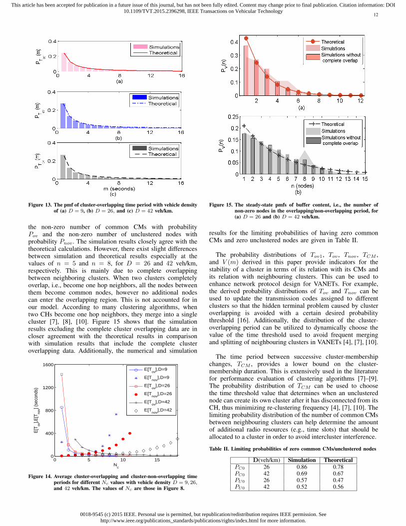
Figure 13 plot the pmfs of the cluster-overlapping, Tovtime period for different vehicle densities when Nc is set tothe average values in Table I8. The time interval betweensuccessive changes of cluster-overlap state is equal to Tov(Tnov) when the two clusters are overlapping (disjoint). Noticethat the vehicle density has little impact on the distributionof the overlapping/non-overlapping periods when Nc is setto the average value. However, this is not true for all Nc.

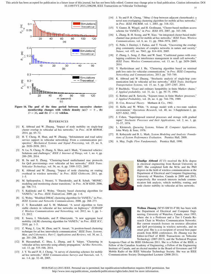
7Figure 16, in the appendix, plots the pmfs of the time interval between twosuccessive cluster-membership changes for different vehicle densities.

8The pmfs of the cluster-non-overlapping, Tnov , follow the same trends. So,the plots are omitted due to space limitations.

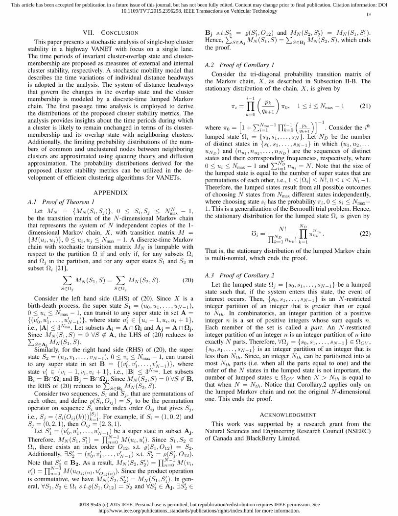
Figure 14 plots the average cluster-overlapping and theaverage cluster-non-overlapping time periods for differentnumbers of nodes between neighbouring clusters, Nc. Theaverage values are calculated using (8) and the values of Ncare from the clustering results in Figure 8. For a fixed Nc,the average cluster-overlapping period is larger for a largerdensity, whereas the average cluster-non-overlapping period issmaller for a larger density. The reason is that, in a congestedtraffic flow conditions, the distance headways are small whencompared to those in an uncongested traffic flow condition.Therefore, for the same Nc, the cumulative distances aresmaller for a high density. It should be noted that the largevalues of average cluster-overlapping time periods for Nc = 1are due to the connected network assumption. Figure 14shows that, as Nc increases, the average cluster-overlappingperiod reduces and the average cluster-non-overlapping periodincreases for the same traffic flow condition.

To investigate the limiting behavior of the number ofvehicles in the overlapping/unclustered region, we firstcalculate the two parameters µ and λ2 for the three vehicledensities. Notice that the distributions (5), (7), and (15) are allconditional on the initial cluster state in terms of Nc and NCM .Therefore, in the calculation of µ and λ2, we use the law oftotal expectation to calculate E[Tov] =

∑n PNc

(n)E[Tov(n)]and E[T 2

Ii] =∑n PNc

(n)E[T 2Ii(n)], where Tov(n) is the

cluster-overlapping time period for two clusters separated byNc = n nodes and TIi(n) is the node interarrival time for acluster with NCM = n nodes, respectively. The calculationsare done for near-capacity and congested traffic flow conditionsonly. The reason is that the diffusion approximation assumesthat the point processes Ni(ζk) and No(θk) are normallydistributed according to the central limit theorem. Thisassumption is not satisfied for an uncongested traffic flow,due to a relatively small number of vehicles between twoclusters as shown in Figure 8. The intensity factor is foundto be ρ = 1.0143 and 1.3172 for D = 26 and 42 veh/km,respectively. As a result, the steady-state distribution doesnot exist. However, consider only Nc ≥ E[Nc] for bothcases, we find that ρ = 0.33, and 0.64 for D = 26, and42 veh/km, respectively. Figure 15 plots the steady-stateprobability distributions for the non-zero number of vehiclesin the overlapping/unclustered region when Nc ≥ E[Nc]for near-capacity and congested traffic flow conditions. Thetheoretical results are normalized to the value 1 − PV (0),since the probability distributions in Figure 15 represent

0 20 40 60 80 1000

0.01

0.02

0.03

0.04

0.05

0.06

0.07

m (seconds)

P T Ii(m)

SimulationsTheoretical exactTheoretical approximation

Figure 12. The pmf of the interarrival time of nodes to the overlappingregion when Nc = 5 and D = 26 veh/km.



12

Figure 13. The pmf of cluster-overlapping time period with vehicle densityof (a) D = 9, (b) D = 26, and (c) D = 42 veh/km.

the non-zero number of common CMs with probabilityPov and the non-zero number of unclustered nodes withprobability Pnov . The simulation results closely agree with thetheoretical calculations. However, there exist slight differencesbetween simulation and theoretical results especially at thevalues of n = 5 and n = 8, for D = 26 and 42 veh/km,respectively. This is mainly due to complete overlappingbetween neighboring clusters. When two clusters completelyoverlap, i.e., become one hop neighbors, all the nodes betweenthem become common nodes, however no additional nodescan enter the overlapping region. This is not accounted for inour model. According to many clustering algorithms, whentwo CHs become one hop neighbors, they merge into a singlecluster [7], [8], [10]. Figure 15 shows that the simulationresults excluding the complete cluster overlapping data are incloser agreement with the theoretical results in comparisonwith simulation results that include the complete clusteroverlapping data. Additionally, the numerical and simulation

0 5 10 150

400

800

1200

1600

Nc

E[T

ov],E

[Tno

v] (se

cond

s)

E[T

ov],D=9

E[Tnov

],D=9

E[Tov

],D=26

E[Tnov

],D=26

E[Tov

],D=42

E[Tnov

],D=42

Figure 14. Average cluster-overlapping and cluster-non-overlapping timeperiods for different Nc values with vehicle density D = 9, 26,and 42 veh/km. The values of Nc are those in Figure 8.

Figure 15. The steady-state pmfs of buffer content, i.e., the number ofnon-zero nodes in the overlapping/non-overlapping period, for(a) D = 26 and (b) D = 42 veh/km.

results for the limiting probabilities of having zero commonCMs and zero unclustered nodes are given in Table II.

The probability distributions of Tov1, Tov , Tnov , TCM ,and V (m) derived in this paper provide indicators for thestability of a cluster in terms of its relation with its CMs andits relation with neighbouring clusters. This can be used toenhance network protocol design for VANETs. For example,the derived probability distributions of Tov and Tnov can beused to update the transmission codes assigned to differentclusters so that the hidden terminal problem caused by clusteroverlapping is avoided with a certain desired probabilitythreshold [16]. Additionally, the distribution of the cluster-overlapping period can be utilized to dynamically choose thevalue of the time threshold used to avoid frequent mergingand splitting of neighbouring clusters in VANETs [4], [7], [10].

The time period between successive cluster-membershipchanges, TCM , provides a lower bound on the cluster-membership duration. This is extensively used in the literaturefor performance evaluation of clustering algorithms [7]–[9].The probability distribution of TCM can be used to choosethe time threshold value that determines when an unclusterednode can create its own cluster after it has disconnected from itsCH, thus minimizing re-clustering frequency [4], [7], [10]. Thelimiting probability distribution of the number of common CMsbetween neighbouring clusters can help determine the amountof additional radio resources (e.g., time slots) that should beallocated to a cluster in order to avoid intercluster interference.

Table II. Limiting probabilities of zero common CMs/unclustered nodes

D(veh/km) Simulation TheoreticalPC0 26 0.86 0.78PC0 42 0.69 0.67PU0 26 0.57 0.47PU0 42 0.52 0.56



13

VII. CONCLUSION

This paper presents a stochastic analysis of single-hop clusterstability in a highway VANET with focus on a single lane.The time periods of invariant cluster-overlap state and cluster-membership are proposed as measures of external and internalcluster stability, respectively. A stochastic mobility model thatdescribes the time variations of individual distance headwaysis adopted in the analysis. The system of distance headwaysthat govern the changes in the overlap state and the clustermembership is modeled by a discrete-time lumped Markovchain. The first passage time analysis is employed to derivethe distributions of the proposed cluster stability metrics. Theanalysis provides insights about the time periods during whicha cluster is likely to remain unchanged in terms of its cluster-membership and its overlap state with neighboring clusters.Additionally, the limiting probability distributions of the num-bers of common and unclustered nodes between neighboringclusters are approximated using queuing theory and diffusionapproximation. The probability distributions derived for theproposed cluster stability metrics can be utilized in the de-velopment of efficient clustering algorithms for VANETs.

APPENDIXA.1 Proof of Theorem 1

Let MN = MN (Si, Sj), 0 ≤ Si, Sj ≤ NNmax − 1,

be the transition matrix of the N -dimensional Markov chainthat represents the system of N independent copies of the 1-dimensional Markov chain, X , with transition matrix M =M(ui, uj), 0 ≤ ui, uj ≤ Nmax − 1. A discrete-time Markovchain with stochastic transition matrix MN is lumpable withrespect to the partition Ω if and only if, for any subsets Ωiand Ωj in the partition, and for any super states S1 and S2 insubset Ωi [21],∑

S∈Ωj

MN (S1, S) =∑S∈Ωj

MN (S2, S). (20)

Consider the left hand side (LHS) of (20). Since X is abirth-death process, the super state S1 = (u0, u1, . . . , uN−1),0 ≤ ui ≤ Nmax − 1, can transit to any super state in set A =(u′0, u′1, . . . , u′N−1), where state u′i ∈ ui − 1, ui, ui + 1,i.e., |A| ≤ 3Nmax . Let subsets Ai = A∩Ωi and Aj = A∩Ωj.Since MN (S1, S) = 0 ∀S 6∈ A, the LHS of (20) reduces to∑S∈Aj

MN (S1, S).Similarly, for the right hand side (RHS) of (20), the super

state S2 = (v0, v1, . . . , vN−1), 0 ≤ vi ≤ Nmax − 1, can transitto any super state in set B = (v′0, v′1, . . . , v′N−1), wherestate v′i ∈ vi − 1, vi, vi + 1, i.e., |B| ≤ 3Nmax . Let subsetsBi = B∩Ωi and Bj = B∩Ωj. Since MN (S2, S) = 0 ∀S 6∈ B,the RHS of (20) reduces to

∑S∈Bj

MN (S2, S).Consider two sequences, Si and Sj , that are permutations of

each other, and define %(Si, Oij) = Sj to be the permutationoperator on sequence Si under index order Oij that gives Sj ,i.e., Sj = (Si(Oij(k)))

|Sj |k=1. For example, if Si = (1, 0, 2) and

Sj = (0, 2, 1), then Oij = (2, 3, 1).Let S′1 = (u′0, u

′1, . . . , u

′N−1) be a super state in subset Aj.

Therefore, MN (S1, S′1) =

∏N−1n=0 M(ui, u

′i). Since S1, S2 ∈

Ωi, there exists an index order O12, s.t. %(S1, O12) = S2.Additionally, ∃S′2 = (v′0, v

′1, . . . , v

′N−1) s.t. S′2 = %(S′1, O12).

Note that S′2 ∈ B2. As a result, MN (S2, S′2) =

∏N−1n=0 M(vi,

v′i) =∏N−1n=0 M(uO12(n), u

′O12(n)). Since the product operation

is commutative, we have MN (S2, S′2) = MN (S1, S

′1). In gen-

eral, ∀S1, S2 ∈ Ωi s.t.%(S1, O12) = S2 and ∀S′1 ∈ Aj, ∃S′2 ∈

Bj s.t.S′2 = %(S′1, O12) and MN (S2, S

′2) = MN (S1, S

′1).

Hence,∑S∈Aj

MN (S1, S) =∑S∈Bj

MN (S2, S), which endsthe proof.

A.2 Proof of Corollary 1Consider the tri-diagonal probability transition matrix of

the Markov chain, X , as described in Subsection II-B. Thestationary distribution of the chain, X , is given by

πi =

i−1∏k=0

(pkqk+1

)π0, 1 ≤ i ≤ Nmax − 1 (21)

where π0 =[1 +

∑Nmax−1i=1

∏i−1k=0

(pkqk+1

)]−1

. Consider the ith

lumped state Ωi = s0, s1, . . . , sN. Let ND be the numberof distinct states in s0, s1, . . . , sN−1 in which (u1, u2, . . .uND

) and (nu1 , nu2 , . . . , nND) are the sequences of distinct

states and their corresponding frequencies, respectively, where0 ≤ ui ≤ Nmax − 1 and

∑ND

i=1 nui= N . Note that the size of

the lumped state is equal to the number of super states that arepermutations of each other, i.e., 1 ≤ |Ωi| ≤ N !, 0 ≤ i ≤ NL−1.Therefore, the lumped states result from all possible outcomesof choosing N states from Nmax different states independently,where choosing state si has the probability πi, 0 ≤ si ≤ Nmax−1. This is a generalization of the Bernoulli trial problem. Hence,the stationary distribution for the lumped state Ωi is given by

fi =N !∏ND

k=1 nuk!

ND∏k=1

πnukuk . (22)

That is, the stationary distribution of the lumped Markov chainis multi-nomial, which ends the proof.

A.3 Proof of Corollary 2Let the lumped state Ωj = s0, s1, . . . , sN−1 be a lumped

state such that, if the system enters this state, the event ofinterest occurs. Then, s0, s1, . . . , sN−1 is an N -restrictedinteger partition of an integer that is greater than or equalto Nth. In combinatorics, an integer partition of a positiveinteger n is a set of positive integers whose sum equals n.Each member of the set is called a part. An N -restrictedinteger partition of an integer n is an integer partition of n intoexactly N parts. Therefore, ∀Ωj = s0, s1, . . . , sN−1 ∈ ΩOV ,s0, s1, . . . , sN−1 is an integer partition of an integer that isless than Nth. Since, an integer Nth can be partitioned into atmost Nth parts (i.e. when all the parts equal to one) and theorder of the N states in the lumped state is not important, thenumber of lumped states ∈ ΩOV when N > Nth is equal tothat when N = Nth. Notice that Corollary.2 applies only onthe lumped Markov chain and not the original N -dimensionalone. This ends the proof.

ACKNOWLEDGMENT

This work was supported by a research grant from theNatural Sciences and Engineering Research Council (NSERC)of Canada and BlackBerry Limited.



14

Figure 16. The pmf of the time period between successive cluster-membership changes with vehicle density (a)D = 9 , (b)D = 26, and (b) D = 42 veh/km.

REFERENCES

[1] K. Abboud and W. Zhuang, “Impact of node mobility on single-hopcluster overlap in vehicular ad hoc networks,” in Proc. ACM MSWiM,2014, pp. 65–72.

[2] H. T. Cheng, H. Shan, and W. Zhuang, “Infotainment and road safetyservice support in vehicular networking: From a communication per-spective,” Mechanical Systems and Signal Processing, vol. 25, no. 6,pp. 2020–2038, 2011.

[3] N. Lu, N. Cheng, N. Zhang, X. Shen, and J. Mark, “Connected vehicles:Solutions and challenges,” IEEE J. Internet of Things, vol. 1, no. 4, pp.289–299, 2014.

[4] H. Su and X. Zhang, “Clustering-based multichannel mac protocolsfor QoS provisionings over vehicular ad hoc networks,” IEEE Trans.Vehicular Technology, vol. 56, no. 6, pp. 3309–3323, 2007.

[5] K. Abboud and W. Zhuang, “Impact of node clustering on routingoverhead in wireless networks,” in Proc. IEEE Globecom, 2011, pp.1–5.

[6] M. Spiliopoulou, I. Ntoutsi, Y. Theodoridis, and R. Schult, “MONIC:modeling and monitoring cluster transitions,” in Proc. ACM KDD, 2006,pp. 706–711.

[7] S. Kuklinski and G. Wolny, “Density based clustering algorithm forVANETs,” in Proc. IEEE TridentCom, 2009, pp. 1–6.

[8] G. Wolny, “Modified DMAC clustering algorithm for VANETs,” in Proc.IEEE Systems and Networks Communications, 2008, pp. 268–273.

[9] Z. Y. Rawashdeh and S. M. Mahmud, “A novel algorithm to formstable clusters in vehicular ad hoc networks on highways,” EURASIPJ. Wireless Communications and Networking, vol. 2012, no. 1, pp. 1–13, 2012.

[10] E. Souza, I. Nikolaidis, and P. Gburzynski, “A new aggregate localmobility (ALM) clustering algorithm for VANETs,” in Proc. IEEE ICC,2010, pp. 1–5.

[11] Z. Wang, L. Liu, M. Zhou, and N. Ansari, “A position-based clusteringtechnique for ad hoc intervehicle communication,” IEEE Trans. Systems,Man, and Cybernetics, Part C: Applications and Reviews, vol. 38, no. 2,pp. 201–208, 2008.

[12] B. Hassanabadi, C. Shea, L. Zhang, and S. Valaee, “Clustering invehicular ad hoc networks using affinity propagation,” Ad Hoc Networks,vol. 13, pp. 535–548, 2014.

[13] J. Y. Yu and P. H. J. Chong, “A survey of clustering schemes for mobilead hoc networks.” IEEE Communications Surveys and Tutorials, vol. 7,no. 1-4, pp. 32–48, 2005.

[14] J. Yu and P. H. Chong, “3hbac (3-hop between adjacent clusterheads): anovel non-overlapping clustering algorithm for mobile ad hoc networks,”in Proc. IEEE PACRIM, vol. 1, 2003, pp. 318–321.

[15] Y. Gunter, B. Wiegel, and H. Großmann, “Cluster-based medium accessscheme for VANETs,” in Proc. IEEE ITS, 2007, pp. 343–348.

[16] L. Zhang, B.-H. Soong, and W. Xiao, “An integrated cluster-based multi-channel mac protocol for mobile ad hoc networks,” IEEE Trans. WirelessCommunications, vol. 6, no. 11, pp. 3964–3974, 2007.

[17] G. Palla, I. Derenyi, I. Farkas, and T. Vicsek, “Uncovering the overlap-ping community structure of complex networks in nature and society,”Nature, vol. 435, no. 7043, pp. 814–818, 2005.

[18] Z. Zhang, L. Song, Z. Han, and W. Saad, “Coalitional games with over-lapping coalitions for interference management in small cell networks,”IEEE Trans. Wireless Communications, vol. 13, no. 5, pp. 2659–2669,2014.

[19] Y. Harikrishnan and J. He, “Clustering algorithm based on minimalpath loss ratio for vehicular communication,” in Proc. IEEE Computing,Networking and Communications, 2013, pp. 745–749.

[20] K. Abboud and W. Zhuang, “Stochastic analysis of single-hop com-munication link in vehicular ad hoc networks,” IEEE Trans. IntelligentTransportation Systems, vol. 15, no. 5, pp. 2297–2307, 2014.

[21] P. Buchholz, “Exact and ordinary lumpability in finite Markov chains,”J. Applied probability, vol. 31, no. 1, pp. 59–75, 1994.

[22] G. Rubino and B. Sericola, “Sojourn times in finite Markov processes,”J. Applied Probability, vol. 26, no. 4, pp. 744–756, 1989.

[23] D. Cox, Renewal Theory. Methuen & Co., 1962.[24] O. Kella and W. Whitt, “A storage model with a two-state random

environment,” Operations Research, vol. 40, no. 3-Supplement-2, pp.S257–S262, 1992.

[25] J. Cohen, “Superimposed renewal processes and storage with gradualinput,” Stochastic Processes and their Applications, vol. 2, no. 1, pp.31–57, 1974.

[26] L. Kleinrock, Queueing Systems, Volume II: Computer Applications.John Wiely & Sons, 1976.

[27] H. Kobayashi and B. L. Mark, System Modeling and Analysis: Founda-tions of System Performance Evaluation. Prentice Hall, 2009.

[28] A. May, Traffic Flow Fundamentals. Prentice Hall, 1990.

Khadige Abboud (S’13) received the B.Sc degreein electrical engineering from Kuwait University in2007. She completed both the M.Sc and the PhDdegrees in the field of wireless communications at theDepartment of Electrical and Computer Engineering,University of Waterloo, Canada in 2009 and 2015,respectively. Her research interests include commu-nication link analysis, vehicle mobility, routing, andnode cluster stability in vehicular ad hoc networks.

Weihua Zhuang (M’93-SM’01-F’08) has been withthe Department of Electrical and Computer Engi-neering, University of Waterloo, Canada, since 1993,where she is a Professor and a Tier I Canada Re-search Chair in Wireless Communication Networks.Her current research focuses on resource allocationand QoS provisioning in wireless networks, and onsmart grid. She is a co-recipient of several best paperawards from IEEE conferences. Dr. Zhuang was theEditor-in-Chief of IEEE Transactions on VehicularTechnology (2007-2013), and the Technical Program

Symposia Chair of the IEEE Globecom 2011. She is a Fellow of the IEEE, aFellow of the Canadian Academy of Engineering, a Fellow of the EngineeringInstitute of Canada, and an elected member in the Board of Governors and VPMobile Radio of the IEEE Vehicular Technology Society. She was an IEEECommunications Society Distinguished Lecturer (2008-2011).

stochastic modeling of single-hop cluster stability in...

Documents