STOCHASTIC HYDROLOGY Lecture -26

Course Instructor : Prof. P. P. MUJUMDAR Department of Civil Engg., IISc.

INDIAN  INSTITUTE  OF  SCIENCE  

2  

Summary  of  the  previous  lecture  

•  Hydrologic data series for frequency analysis –  Complete duration series –  Partial duration series –  Annual exceedence series –  Extreme value series

•  Extreme value distributions •  Frequency factors

Frequency factor for Normal Distribution:

3  

Frequency Analysis

T T

TT

x KxK

µ σ

µσ

= +

−=

12

2

1lnwp

⎡ ⎤⎛ ⎞= ⎢ ⎥⎜ ⎟

⎝ ⎠⎣ ⎦0 < p < 0.5

2

2 3

2.515517 0.802853 0.0103281 1.432788 0.189269 0.001308T

w wK ww w w+ +

= −+ + +

Consider the annual maximum discharge Q in cumec, of a river for 45 years :

4  

Example – 1

Year Q Year Q Year Q Year Q 1950 804 1961 507 1972 1651 1983 1254 1951 1090 1962 1303 1973 716 1984 430 1952 1580 1963 197 1974 286 1985 260 1953 487 1964 583 1975 671 1986 276 1954 719 1965 377 1976 3069 1987 1657 1955 140 1966 348 1977 306 1988 937 1956 1583 1967 804 1978 116 1989 714 1957 1642 1968 328 1979 162 1990 855 1958 1586 1969 245 1980 425 1991 399 1959 218 1970 140 1981 1982 1992 1543 1960 623 1971 49 1982 277 1993 360

1994 348

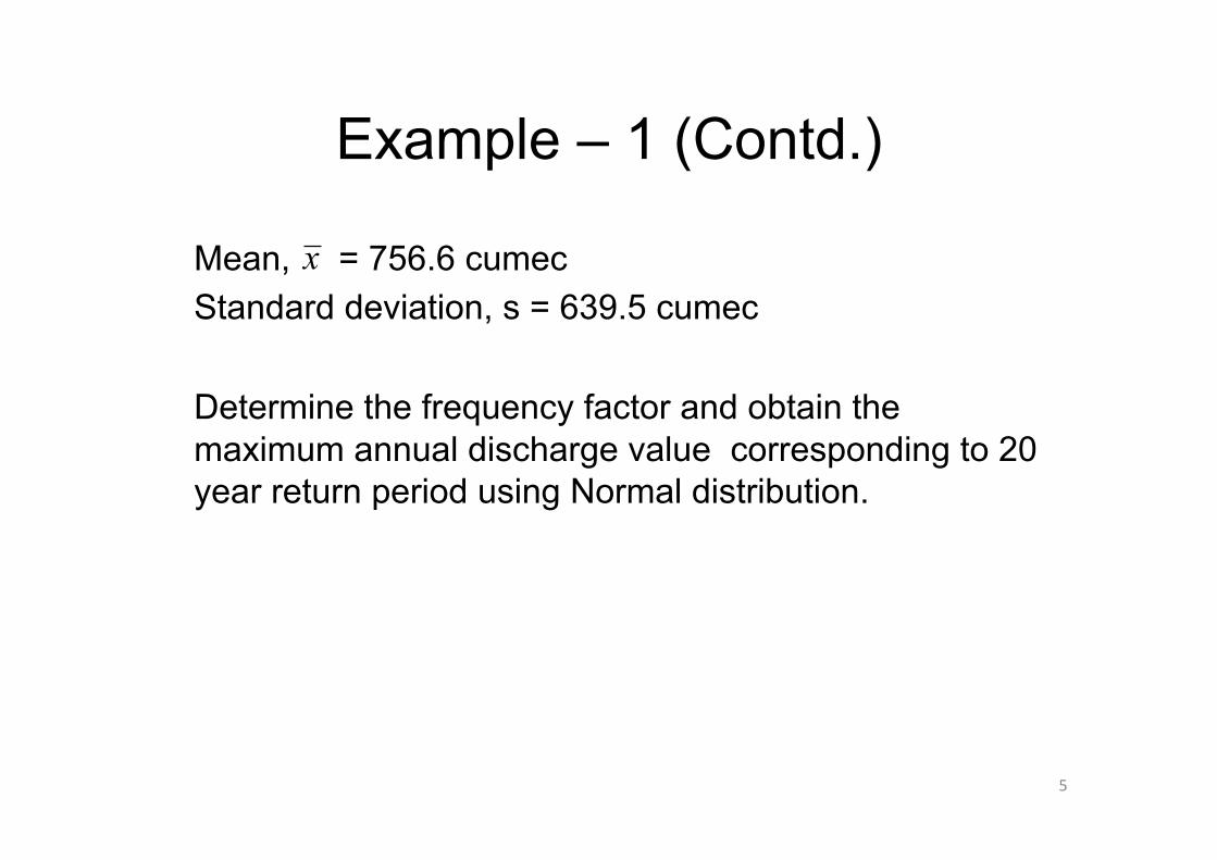
Mean, = 756.6 cumec Standard deviation, s = 639.5 cumec Determine the frequency factor and obtain the maximum annual discharge value corresponding to 20 year return period using Normal distribution.

5  

Example – 1 (Contd.)

x

T = 20 p = 1/20 = 0.05

6  

Example – 1 (Contd.)

12

2

12

2

1ln

1ln0.05

2.45

wp

⎡ ⎤⎛ ⎞= ⎢ ⎥⎜ ⎟

⎝ ⎠⎣ ⎦

⎡ ⎤⎛ ⎞= ⎜ ⎟⎢ ⎥⎝ ⎠⎣ ⎦

=

cumec

7  

Example – 1 (Contd.) 2

20 2 3

2

2 3

2.515517 0.802853 0.010321 1.432788 0.189269 0.001308

2.515517 0.802853 2.45 0.01032 2.452.451 1.432788 2.45 0.189269 2.45 0.001308 2.45

1.648

w wK ww w w+ +

= −+ + +

+ × + ×= −

+ × + × + ×=

20 20

756.6 1.648 639.51810.5

x x K s= +

= + ×

=

Frequency factor for Extreme Value Type I (EV I) Distribution:

•  To express T in terms of KT,

8  

Frequency Analysis

6 0.5772 ln ln1T

TKTπ

⎧ ⎫⎡ ⎤⎛ ⎞= − +⎨ ⎬⎜ ⎟⎢ ⎥−⎝ ⎠⎣ ⎦⎩ ⎭

1

1 exp exp 0.57726T

TKπ

=⎧ ⎫⎡ ⎤⎛ ⎞⎪ ⎪

− − − +⎨ ⎬⎢ ⎥⎜ ⎟⎝ ⎠⎪ ⎪⎣ ⎦⎩ ⎭

Ref: Applied Hydrology by V.T.Chow, D.R.Maidment, L.W.Mays, McGraw-Hill 1998

When xT = µ in the equation ; KT = 0 Substituting KT = 0, i.e., the return period of mean of a EV I is 2.33 years

9  

Frequency Analysis

TT

xK µσ−

=

101 exp exp 0.57726

2.33

Tπ

=⎧ ⎫⎡ ⎤×⎛ ⎞⎪ ⎪

− − − +⎨ ⎬⎢ ⎥⎜ ⎟⎝ ⎠⎪ ⎪⎣ ⎦⎩ ⎭

= years

T Tx Kµ σ= +

Consider the annual maximum discharge of a river for 45 years, given in the previous example. Mean, = 756.6 cumec Standard deviation, s = 639.5 cumec Determine the frequency factor and obtain the maximum annual discharge value corresponding to 20 year return period using Extreme Value Type I (EV I) distribution.

10  

Example – 2

x

T = 20 years

11  

Example – 2 (Contd.)

6 0.5772 ln ln1

6 200.5772 ln ln20 1

1.866

TTKTπ

π

⎧ ⎫⎡ ⎤⎛ ⎞= − +⎨ ⎬⎜ ⎟⎢ ⎥−⎝ ⎠⎣ ⎦⎩ ⎭

⎧ ⎫⎡ ⎤⎛ ⎞= − +⎨ ⎬⎜ ⎟⎢ ⎥−⎝ ⎠⎣ ⎦⎩ ⎭=

756.6 1.866 639.51949.9

T Tx x K s= +

= + ×

= cumec

Frequency factor for Log Pearson Type III Distribution: The PDF is

where y = log x

•  The data is converted to the logarithmic series by {y} = log {x}.

12  

Frequency Analysis

( ) ( ) ( )

( )

1 yy ef x

x

β λ εβλ ε

β

− − −−=

Γlog x ε≥

•  The mean , standard deviation sy, and the coefficient of skewness Cs are calculated for the converted logarithmic series {y}

•  The frequency factor for the log Pearson Type III distribution depends on the return period and coefficient of skewness

13  

Frequency Analysis

y

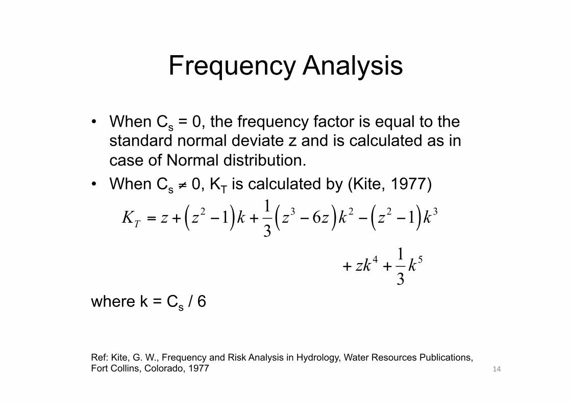
•  When Cs = 0, the frequency factor is equal to the standard normal deviate z and is calculated as in case of Normal distribution.

•  When Cs ≠ 0, KT is calculated by (Kite, 1977)

where k = Cs / 6

14  

Frequency Analysis

( ) ( ) ( )2 3 2 2 3

4 5

11 6 13

13

TK z z k z z k z k

zk k

= + − + − − −

+ +

Ref: Kite, G. W., Frequency and Risk Analysis in Hydrology, Water Resources Publications, Fort Collins, Colorado, 1977

Consider the annual maximum discharge of a river for 45 years given in the previous example. Calculate the frequency factor and obtain the maximum annual discharge value corresponding to 20 year return period using Log Person Type III distribution. The logarithmic data series is first obtained.

15  

Example – 3

Logarithmic values of the data given in the previous example:

16  

Example – 3 (Contd.)

Year Log Q Year Log Q Year Log Q Year Log Q 1950 2.905 1961 2.705 1972 3.218 1983 3.098 1951 3.037 1962 3.115 1973 2.855 1984 2.633 1952 3.199 1963 2.294 1974 2.456 1985 2.415 1953 2.688 1964 2.766 1975 2.827 1986 2.441 1954 2.857 1965 2.576 1976 3.487 1987 3.219 1955 2.146 1966 2.542 1977 2.486 1988 2.972 1956 3.199 1967 2.905 1978 2.064 1989 2.854 1957 3.215 1968 2.516 1979 2.210 1990 2.932 1958 3.200 1969 2.389 1980 2.628 1991 2.601 1959 2.338 1970 2.146 1981 3.297 1992 3.188 1960 2.794 1971 1.690 1982 2.442 1993 2.556

1994 2.542

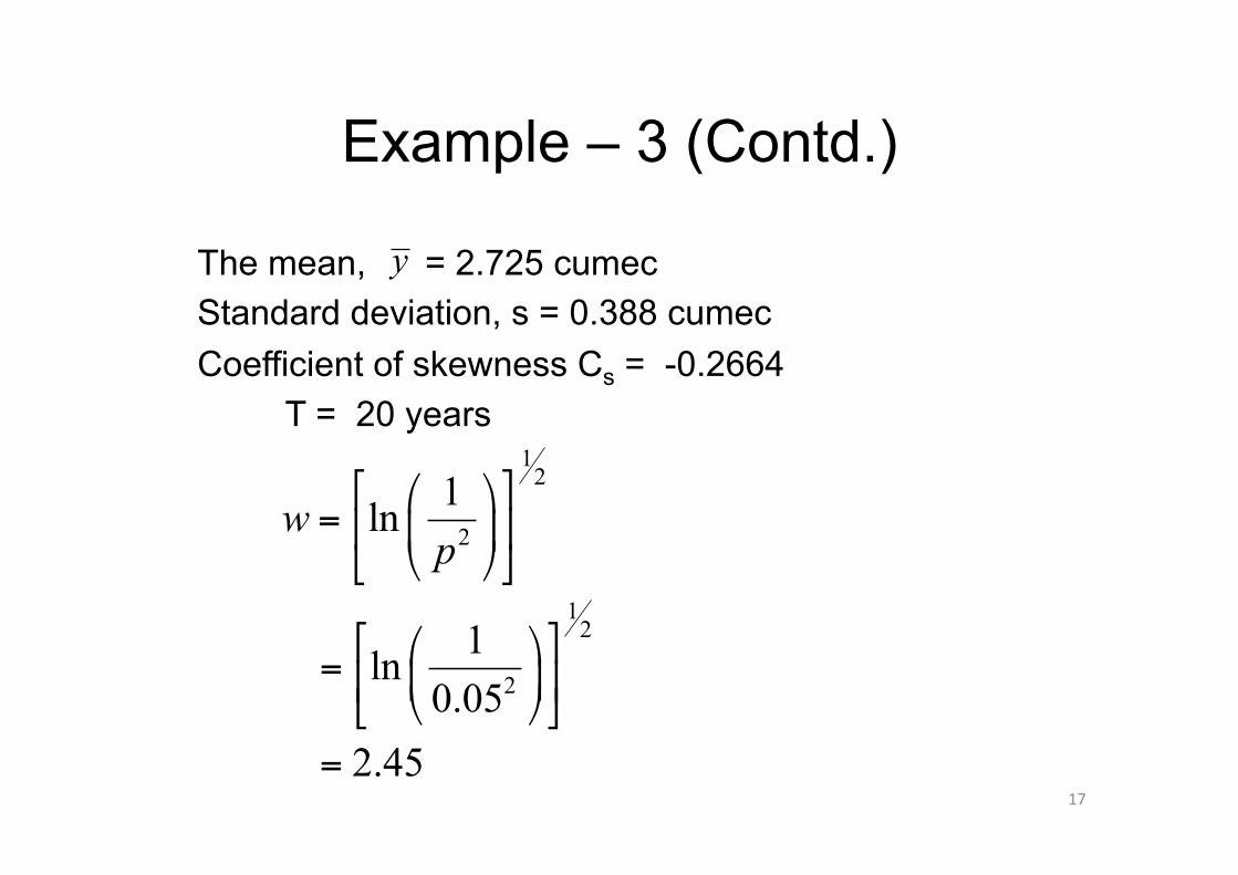
The mean, = 2.725 cumec Standard deviation, s = 0.388 cumec Coefficient of skewness Cs = -0.2664 T = 20 years

17  

Example – 3 (Contd.)

y

12

2

12

2

1ln

1ln0.05

2.45

wp

⎡ ⎤⎛ ⎞= ⎢ ⎥⎜ ⎟

⎝ ⎠⎣ ⎦

⎡ ⎤⎛ ⎞= ⎜ ⎟⎢ ⎥⎝ ⎠⎣ ⎦

=

18  

Example – 3 (Contd.) 2

2 3

2

2 3

2.515517 0.802853 0.010321 1.432788 0.189269 0.001308

2.515517 0.802853 2.45 0.01032 2.452.451 1.432788 2.45 0.189269 2.45 0.001308 2.45

1.648

w wz ww w w+ +

= −+ + +

+ × + ×= −

+ × + × + ×=

k = Cs / 6 = -0.2664/6 = -0.0377

= 1.581

19  

Example – 3 (Contd.)

756.6 1.581 639.51767.6

T Tx x K s= +

= + ×

= cumec

( )( ) ( )( )

( )( ) ( ) ( )

22 3

3 4 52

11.648 1.648 1 0.0377 1.648 6 1.648 0.03773

11.648 1 0.0377 1.648 0.0377 0.03773

TK = + − − + − × −

− − − + × − + −

PROBABILITY PLOTTING

•  Probability plotting is a method to check whether a probability distribution fits a set of data or not.

•  The data is plotted on specially designed probability paper.

•  When the cumulative distribution function (CDF) F(x), is plotted on arithmetic paper versus the value of RV X, usually a straight line does not result.

•  To obtain a straight line on arithmetic paper, F(x) would have to be given by expression F(x) = ax+b or f(x) = a; which is an uniform distribution

21  

Probability Plotting

i.e., if a CDF of a set of data plots a straight line on arithmetic paper, the data follows uniform distribution.

•  The probability paper for a given distribution can be developed so that the cumulative distribution plots as a straight line on the paper.

22  

Probability Plotting

•  Constructing probability paper is a process of transforming the arithmetic scale to the probability scale so that the resulting cumulative distribution plot is a straight line

•  The plot is prepared with exceedence probability or the return period ‘T’ on abscissa and the magnitude of the event on ordinate.

23  

Probability Plotting

Construction of Probability paper: •  Mathematical construction. •  Graphical construction

24  

Probability Plotting

Mathematical construction: •  For some probability distributions, probability paper

can be constructed analytically so that the cumulative distribution function plots a straight line, on the paper.

•  This can be achieved by transforming the cumulative distribution function to the form where Y is a function of parameters and F(x), Z is a function of parameters and x, a and b are functions of parameters.

25  

Probability Plotting

Y aZ b= +

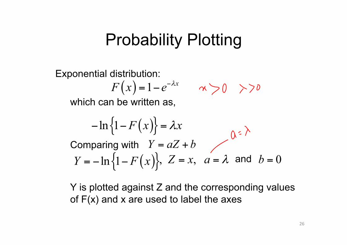
Exponential distribution: which can be written as, Comparing with and Y is plotted against Z and the corresponding values of F(x) and x are used to label the axes

26  

Probability Plotting

( ) 1 xF x e λ−= −

( ){ }ln 1 F x xλ− − =

Y aZ b= +

( ){ }ln 1Y F x= − − , , 0Z x a bλ= = =

Construct probability paper for exponential distribution with λ = 1/3 Soln: 1.  The values of F(x) are assumed and corresponding

x, Y and Z values are calculated. 2.  Y is plotted against Z and the Y axis is labeled with

the corresponding value of F(x) and the Z axis with corresponding value of x.

27  

Example – 4

28  

Example – 4 (Contd.) F(x) Y x = Z 0.01 0.010 0.030 0.05 0.051 0.154 0.1 0.105 0.316 0.2 0.223 0.669 0.3 0.357 1.070 0.4 0.511 1.532 0.5 0.693 2.079 0.6 0.916 2.749 0.7 1.204 3.612 0.8 1.609 4.828 0.9 2.303 6.908

0.95 2.996 8.987 0.99 4.605 13.816

Y is plotted against Z :

29  

Example – 4 (Contd.)

0  

1  

2  

3  

4  

5  

0   3   6   9   12   15  

Y  

Z  

Y axis labeled with F(x) and Z with x :

30  

Example – 4 (Contd.)

0.99  

0.7  0.8  

0.9  

0.95  

0.5  

0.1  

F(x)  

X  =  

Probability paper for exponential distribution:

31  

Example – 4 (Contd.)

0.99  

0.7  0.8  

0.9  

0.95  

0.5  

0.1  

F(x)  

X  

0   9   12   15  3   6  

Probability paper for exponential distribution:

32  

Example – 4 (Contd.)

0.99  

0.7  0.8  

0.9  

0.95  

0.5  

0.1  

F(x)  

X  

0   9   12   15  3   6  

λ1 λ2

•  Any exponential distribution data will plot as a straight line .

•  The slope of the line will change as λ changes. •  Slope of the line gives the λ value. •  For many probability distributions, the same graph

paper may be used for all values of the parameters of the distribution.

•  For some distributions like gamma, a separate graph paper is required for different values of the parameters.

•  Many types of probability papers are commercially available.

33  

Probability Plotting

Graphical construction: •  Graphical construction is done by transforming the

arithmetic scale to probability scale so that a straight line is obtained when cumulative distribution function is plotted

•  The transformation technique is explained with the normal distribution.

•  Consider the coordinates from the standardized normal distribution table.

34  

Probability Plotting

35  

z 0 2 4 6 8 0 0 0.008 0.016 0.0239 0.0319

0.1 0.0398 0.0478 0.0557 0.0636 0.0714 0.2 0.0793 0.0871 0.0948 0.1026 0.1103 0.3 0.1179 0.1255 0.1331 0.1406 0.148 0.4 0.1554 0.1628 0.17 0.1772 0.1844 0.5 0.1915 0.1985 0.2054 0.2123 0.219 0.6 0.2257 0.2324 0.2389 0.2454 0.2517 0.7 0.258 0.2642 0.2704 0.2764 0.2823 0.8 0.2881 0.2939 0.2995 0.3051 0.3106 0.9 0.3159 0.3212 0.3264 0.3315 0.3365 1 0.3413 0.3461 0.3508 0.3554 0.3599

Normal Distribution Tables

z

Normal distribution table:

36  

Probability Plotting

Z F(z)

-3 0.0013

-2.5 0.0062

-2 0.0227

-1.5 0.0668

-1 0.1587

-0.5 0.3085

Z F(z)

0 0.5

0.5 0.6915

1 0.8413

1.5 0.9332

2 0.9772

2.5 0.9938

3 0.9987

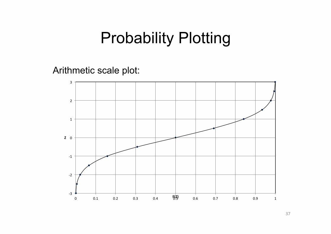
Arithmetic scale plot:

37  

Probability Plotting

-­‐3  

-­‐2  

-­‐1  

0  

1  

2  

3  

0   0.1   0.2   0.3   0.4   0.5   0.6   0.7   0.8   0.9   1  

Z  

F(Z)  

0.1   0.2   0.4   0.5   0.6  0.05   0.7   0.8   0.95  0.9   0.99  0.01  

Transformation plot:

38  

Probability Plotting

0.3  

F(Z)

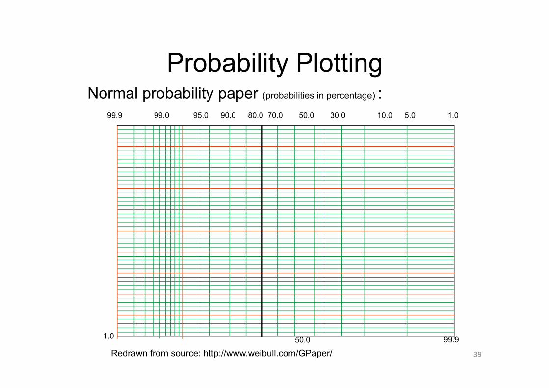
Normal probability paper (probabilities in percentage) :

39  

Probability Plotting

99.9 99.0 95.0 90.0 80.0 70.0 50.0 30.0 10.0 5.0 1.0

1.0 50.0 99.9

Redrawn from source: http://www.weibull.com/GPaper/

•  The purpose of using the probability paper is to linearize the probability relationship

•  The plot can be used for interpolation, extrapolation and comparison purposes.

•  The plot can also be used for estimating magnitudes with other return periods.

•  If the plot is used for extrapolation, the effect of various errors is often magnified.

40  

Probability Plotting

•  Plotting position is a simple empirical technique •  Relation between the magnitude of an event verses

its probability of exceedence. •  Plotting position refers to the probability value

assigned to each of the data to be plotted •  Several empirical methods to determine the plotting

positions. •  Arrange the given series of data in descending

order •  Assign a order number to each of the data (termed

as rank of the data)

41  

Plotting Position

•  First entry as 1, second as 2 etc. •  Let ‘n’ is the total no. of values to be plotted and ‘m’ is the rank of a value, the exceedence probability (p) of the mth largest value is obtained by various formulae.

•  The return period (T) of the event is calculated by T = 1/p

•  Compute T for all the events •  Plot T verses the magnitude of event on semi log or

log log paper

42  

Plotting Position

Formulae for exceedence probability: California Method: Limitations –  Produces a probability of 100% for m = n

43  

Plotting Position

( )mmP X xn

≥ =

Modification to California Method: Limitations –  Formula does not produce 100% probability –  If m = 1, probability is zero

44  

Plotting Position

( ) 1m

mP X xn−

≥ =

Hazen’s formula: Chegodayev’s formula: Widely used in U.S.S.R and Eastern European

countries 45  

Plotting Position

( ) 0.5m

mP X xn−

≥ =

( ) 0.30.4m

mP X xn−

≥ =+

Weibull’s formula: –  Most commonly used method –  If ‘n’ values are distributed uniformly between 0

and 100 percent probability, then there must be n+1 intervals, n–1 between the data points and 2 at the ends.

–  Indicates a return period T one year longer than the period of record for the largest value

46  

Plotting Position

( )1m

mP X xn

≥ =+

Most plotting position formulae are represented by:

Where b is a parameter

–  E.g., b = 0.5 for Hazen’s formula, b = 0.5 for Chegodayev’s formula, b = 0 for Weibull’s formula

–  b = 3/8 0.5 for Blom’s formula –  b = 1/3 0.5 for Tukey’s formula –  b = 0.44 0.5 for Gringorten’s formula

47  

Plotting Position

( )1 2mm bP X xn b

−≥ =

+ −

–  Cunnane (1978) studied the various available plotting position methods based on unbiasedness and minimum variance criteria.

–  If large number of equally sized samples are plotted, the average of the plotted points foe each value of m lie on the theoretical distribution line.

–  Minimum variance plotting minimizes the variance of the plotted points about the theoretical line.

–  Cunnane concluded that the Weibull’s formula is biased and plots the largest values of a sample at too small a return period.

48  

Plotting Position

–  For normally distributed data, the best formula is Blom’s plotting position formula (b = 3/8).

–  For Extreme Value Type I distribution, the Gringorten formula (b = 0.44) is the best.

49  

Plotting Position

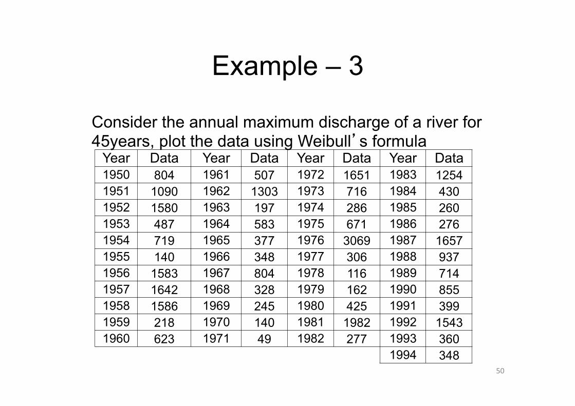
Consider the annual maximum discharge of a river for 45years, plot the data using Weibull’s formula

50  

Example – 3

Year Data Year Data Year Data Year Data 1950 804 1961 507 1972 1651 1983 1254 1951 1090 1962 1303 1973 716 1984 430 1952 1580 1963 197 1974 286 1985 260 1953 487 1964 583 1975 671 1986 276 1954 719 1965 377 1976 3069 1987 1657 1955 140 1966 348 1977 306 1988 937 1956 1583 1967 804 1978 116 1989 714 1957 1642 1968 328 1979 162 1990 855 1958 1586 1969 245 1980 425 1991 399 1959 218 1970 140 1981 1982 1992 1543 1960 623 1971 49 1982 277 1993 360

1994 348

•  The data is arranged in descending order •  Rank is assigned to the arranged data •  The probability is obtained using

•  Return period is calculated •  The maximum annual discharge verses the return

period is plotted

51  

Example – 3 (Contd.)

( )1m

mP X xn

≥ =+

52  

Example – 3 (Contd.) Year Annual

Max. Q Arranged

data Rank (m) P(X > xm) T

1950 804 3069 1 0.021739 46

1951 1090 1982 2 0.043478 23

1952 1580 1657 3 0.065217 15.33333

1953 487 1651 4 0.086957 11.5

1954 719 1642 5 0.108696 9.2

1955 140 1586 6 0.130435 7.666667

1956 1583 1583 7 0.152174 6.571429

1957 1642 1580 8 0.173913 5.75

1958 1586 1543 9 0.195652 5.111111

1959 218 1303 10 0.217391 4.6

1960 623 1254 11 0.23913 4.181818

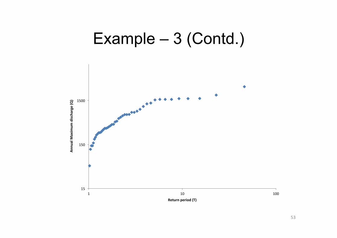
53  

Example – 3 (Contd.)

15  

150  

1500  

1   10   100  

Annu

al  M

axim

um  discharge  (Q

)  

Return  period  (T)