stochastic equations in hilbert space with l©vy noise and their
TRANSCRIPT

Stochastic Equationsin Hilbert Space with Levy Noiseand their Applications in Finance
Diplomarbeitvorgelegt von Stefan Stolze
im StudiengangWirtschaftsmathematik
Fakultaten furMathematik und Wirtschaftswissenschaften
Universitat BielefeldJuli 2005

ii
Contents
Introduction 1
1 Infinitely Divisible Measures 91.1 The Bochner Integral . . . . . . . . . . . . . . . . . . . . . . . 91.2 Definition of Infinitely Divisible Measures . . . . . . . . . . . 121.3 Exponents of Levy Measures . . . . . . . . . . . . . . . . . . 151.4 Levy-Khinchin Representation . . . . . . . . . . . . . . . . . 20
2 Levy Processes in Hilbert Space 252.1 Martingales in Hilbert Space . . . . . . . . . . . . . . . . . . 262.2 Gaussian Measures on Hilbert Space . . . . . . . . . . . . . . 292.3 Levy Processes and Poisson Random Measure . . . . . . . . . 312.4 The Levy Ito Decomposition . . . . . . . . . . . . . . . . . . 362.5 Martingale Measures . . . . . . . . . . . . . . . . . . . . . . . 41
3 Stochastic Integration 493.1 Strong Stochastic Integrals . . . . . . . . . . . . . . . . . . . 503.2 Weak Stochastic Integrals . . . . . . . . . . . . . . . . . . . . 573.3 Properties of the Stochastic Integral . . . . . . . . . . . . . . 62
4 Stochastic Equations with Levy Noise 694.1 The Stochastic Convolution . . . . . . . . . . . . . . . . . . . 714.2 Ornstein-Uhlenbeck Type Processes . . . . . . . . . . . . . . 794.3 Lipschitz Nonlinearities . . . . . . . . . . . . . . . . . . . . . 83
5 Applications in Finance 895.1 The classical Black-Scholes Model . . . . . . . . . . . . . . . . 905.2 Asset Price Models with Levy Processes . . . . . . . . . . . . 935.3 Generalized Hyperbolic Levy Motions . . . . . . . . . . . . . 955.4 Stochastic Volatility . . . . . . . . . . . . . . . . . . . . . . . 99
Symbols 103
Bibliography 105
iii

iv CONTENTS

Introduction
In this diploma thesis we will solve a stochastic partial differential equationwith Lipschitz nonlinearities where the noise is a Hilbert space valued Levyprocess. We will also present applications of Levy processes in Finance, inparticular in stochastic volatility models. The solution of the mentionedequation may be useful to further improve such models which are up to nowmainly based on Ornstein-Uhlenbeck type processes.
Levy process have in recent time become more and more important inFinance applications. They have for example been used to model the volatil-ity which is implicitly given in financial time series. In a model suggestedby O. E. Barndorff-Nielsen and N. Shepard [BN-S] the stochastic volatilityprocess is an Ornstein-Uhlenbeck type process, i.e. a solution to
dy(t) = ay(t)dt+ bdx(t)
on R1 (or finite combinations of those). Here a, b are real constants andx is a Levy process on R1. Due to the large number of influencing factorsit seems to be more appropriate to construct such processes on an infinitedimensional state space. We will therefore construct a weak solution of theanalogous equation on a separable Hilbert space H, i.e.
dY (t) = JY (t)dt+ CdX(t)Y (0) = Y0.
Here X is Levy process on H, C a bounded linear operator on H and J the,possibly unbounded, generator of a C0-semigroup on H. For a better fit toobserved implied volatility data it might be useful to add a nonlinear termin this equation (see the discussion in section 5.4). Therefore we will extendthe equation to
dY (t) = (JY (t) + F (Y (t)))dt+ CdX(t)Y (0) = Y0,
where F : H → H is a function that fulfills a Lipschitz condition. InTheorem 4.3.3 we will show that under condition (4.1) (cf. chapter 4) thisequation has a unique mild solution and furthermore that this mild solution
1

2 CONTENTS
is also a weak solution. This result is, as far as we know, new for noises thatare Levy processes with values in a separable Hilbert space. It is also thecentral result in this diploma thesis.
In the following chapters we will first give an overview of the theory ofLevy process and infinitely divisible distributions. Afterwards we present theconstruction of the stochastic integral with respect to a martingale measure.Then we turn to stochastic partial differential equations and prove the abovedescribed existence and uniqueness result. Finally we give an insight toapplications of Levy processes in Finance. A more detailed description ofthe single chapters and sections will follow further below.
The stochastic integral will be constructed with respect to a Hilbertspace-valued martingale measure. Levy processes as integrators are an im-portant special case. Real-valued martingale measures were introduced by J.B. Walsh [Wal] in order to solve stochastic partial differential equations. Amartingale measure is a mapping M : [0, t]×S×Ω → R where [0, t] is a timeinterval, (Ω,F , P ) some probability space and S a Lusin topological space.Simply speaking M is a martingale in the time component and a σ-finitemeasure in the S-component. N. El Karoui and S. Meleard [ElKMel] alsostudied vector-valued martingale measures. In [App b] by D. Applebauma corresponding definition of martingale measures with values in a separa-ble Hilbert space was given (therein called martingale-valued measures). Ofspecial interest are martingale measures that fulfill a certain orthogonalitycondition and have a covariance structure that can be described by a familyof trace class operators. (For further details and definitions see section 2.5).The Levy martingale measure, which corresponds to a Levy process, has allof these properties. We will focus on this example and show all importantresults for the Levy martingale measure. Moreover we give a detailed reviewof martingale measures in general (see section 2.5).
Real valued stochastic integrals with Hilbert space-valued martingales asintegrators were constructed by H. Kunita [Kun]. We will refer to this as theweak stochastic integral, since for simple functions it is a sum of inner prod-ucts of integrands with increments of the martingale. Consequently thereis also a strong stochastic integral : This integral takes values in the sameHilbert space as the integrator. The integrands are mappings with imagesin a certain class of linear operators. For the case where the martingales arecontinuous this kind of integral was constructed by B.L. Rozovskii [Roz].More general is the construction of M. Metivier [Met]. Here the integratorsare allowed to be semimartingales and discontinuous. Both types of stochas-tic integrals, the weak and the strong one, are Ito integrals in the sensethat they are defined as L2-limits of the integrals of simple functions whichapproximate the integrand in a proper L2-space. Another approach is todefine the stochastic integral as a limit in distribution. This was done by A.Chojnowska-Michalik [ChM] for the semimartingales being Levy processesand with deterministic integrands. A stochastic integral with respect to

CONTENTS 3
martingale measures has already been developed in [Wal] for the real-valuedcase. In [App b] this construction was carried forward to Hilbert spaces, i.e.martingale measures and integrands are both Hilbert space-valued.
We turn back to the equation from above and add a time dependentdrift:
dY (t) = (JY (t) + f(t))dt+ CdX(t) (1)Y (0) = Y0.
Again X is an H-valued Levy process, where H shall denote a Hilbert spacewhich will be our state space. For some ε > 0 we impose the condition
sup0≤t≤T
‖∆X(t)‖ ∈ L2+ε(R) = L2+ε(Ω → R)
on X, which is thereby in L2(H) = L2(Ω → H) at any time 0 ≤ t ≤ T . Jis the, possibly unbounded generator, of a C0-semigroup (S(t), t ≥ 0) on Hand C a bounded linear operator on H. f : [0, T ] → L2(H) is an adaptedstochastic process, which is Bochner integrable on [0, T ], and Y0 ∈ L2(H) isa random initial value. We will construct a weak solution of this equation.Y : [0, T ] → L2(H) is a weak solution of (1) if Y is Bochner integrable on[0, T ] and for each y ∈ D(J∗) and every t ∈ [0, T ]
(Y (t)− Y0, y)H
=∫ t
0((Y (s), J∗y)H + (f(s), y)H)ds+ (X(t), C∗y)H .
(Here (·, ·)H denotes the inner product in H).In the case that the integrator X is a Brownian motion this equation was
studied by G. Da Prato and J. Zabczyk in [DaPrZa], Chapter 5. They showexistence and uniqueness of a weak solution. For f ≡ 0 the solution of (1)is called Ornstein-Uhlenbeck process. A. Chojnowska-Michalik [ChM] hasfirst studied this equation for an integrator X being a Hilbert space-valuedLevy process. A unique weak solution (therein called mild solution) is con-structed. The same result was obtained by D. Applebaum [App b] usingalternative methods. As mentioned above the stochastic integral with re-spect to martingale measures is constructed there. The solution of equation(1) is then found based on this integration theory. It is worth to mentionthat this approach has the advantage that the Levy Ito decomposition is pre-served within the structure of the solution. We will pick up this constructionin this diploma thesis and fully work out the argumentation. Furthermorein our equation we will also allow the additional drift term f .
Now we discuss the fundamentally new result. Compared with equation(1) the situation is more complicated if non-linear drift terms are introduced.

4 CONTENTS
We consider the following equation with a Lipschitz drift:
dY (t) = (JY (t) + F (Y (t)))dt+ CdX(t) (2)Y (0) = Y0.
The mapping F : H → H is measurable and Lipschitz on [0, T ]. Again we areinterested in a weak solution, i.e. a stochastic process Y : [0, T ] → L2(H),Bochner integrable on [0, T ], such that for all y ∈ D(J∗) and all t ∈ [0, T ]
(Y (t)− Y0, y)H
=∫ t
0((Y (s), J∗y)H + (F (Y (s)), y)H)ds+ (X(t), C∗y)H .
The idea is, to show existence of a mild solution, i.e. a stochastic process Ywith
Y (t) = S(t)Y0 +∫ t
0S(t− s)F (Y (s))ds+
∫ t
0S(t− s)CdX(s). (3)
It is then obtained that in our case a mild solution is also a weak solution.For a Gaussian noise X problem (2) was also examined in [DaPrZa] (seeChapter 7). For non-Gaussian noise these equations have recently beenstudied, but mainly in the real-valued case. S. Albeverio, J.-L. Wu and T.-S. Zhang [AlWuZh] give the solution to an equation of the type (2) (alsoallowing a non-constant diffusion coefficient) driven by a pure Poisson noise.Poisson noise usually is a compensated Poisson random measure (which is anexample for a real-valued martingale measure; for the definition see section2.3). One should also mention C. Muller [Mul] and D. Applebaum and J.-L.Wu [AppWu], where the latter also allow for a Gaussian part in the noise.C. Knoche [Kno a] studies (2) (with non-constant diffusion coefficient) onan infinite dimensional Hilbert space where the integrator is a compensatedPoisson random measure (see also [Kno b]).
To our knowledge there are no results on the equation (2) on infinitedimensional Hilbert spaces where the integrator is a general Levy processwith values in the same Hilbert space. We will show in this diploma thesisthat this equation has a unique weak solution, which is the central result.This is done in the framework of [App b], where the stochastic integral isconstructed with respect to Hilbert space-valued martingale measures. Weare able to show existence and uniqueness of a weak solution to (2) undercertain condition. This condition is the already mentioned condition on thejumps of the Levy process X: For some ε > 0
sup0≤t≤T
‖∆X(t)‖ ∈ L2+ε(R) = L2+ε(Ω → R). (4)
Our proof (see section 4.3) uses a fixed point argument.

CONTENTS 5
We will now give an overview over the single chapters of this diplomathesis with special emphasis on contributions which are new compared tothe literature cited above. Apart from the description here we also referto the more detailed introductions at the beginning of every chapter. InChapter 1 the theory of infinitely divisible measures is developed. An un-derstanding of infinitely divisible measures is important in the study of Levyprocesses as such measures are the distributions of the increments of Levyprocesses. The results presented here are mainly taken from [Lin]. The mostimportant one is the Levy Khinchin Representation (section 1.4) by whichevery infinitely divisible measure can be decomposed into a Dirac measure,a Gaussian measure and a “jump”-part given by the generalized exponentof a Levy measure.
Levy processes on a separable Hilbert space H will be studied in Chap-ter 2. We will first give some useful properties of H-valued martingalesand mention some results for the Gaussian case before we come to generalLevy processes in section 2.3. Given a Levy process X we introduce thecorresponding Poisson random measure and the compensated Poisson ran-dom measure which in the time component is a martingale. Following theapproach of S. Albeverio and B. Rudiger [AlRu] we construct an integralwith respect to the compensated Poisson random measure with determin-istic functions as integrands. We will also cite their main result in thementioned paper: the Levy Ito decomposition on a separable Hilbert space(therein shown for general separable Banach spaces). In the final sectionof this chapter we will extend the definition of martingale measures to theHilbert space case. As mentioned this extension was first done in [App b]and therefore we have taken most of the definitions from there. Note that wewill use a slightly different definition of orthogonality for martingale mea-sures (compare the introduction to the chapter). A very important example- and we will show that it really is an example - is the Levy martingalemeasure, since it describes the martingale part of a Levy process. Of specialinterest are nuclear martingale measures which in the martingale compo-nent have covariance operators that are non-negative self-adjoint and traceclass. Each Levy martingale measure has this property which is also provedin detail.
In Chapter 3 stochastic integrals with respect to nuclear martingale mea-sures are introduced. For the real-valued case this was also done in [Wal].The construction in the H-valued situation follows the ideas of [App b].However some details were left out there and we will give the precise argu-mentation here. First we construct the strong stochastic integral, where theintegrands are certain operator-valued mappings, by an isometry. Next wewill also introduce the real-valued weak stochastic integral (in section 3.2)with H-valued integrands. The construction is quite similar to the one ofthe strong stochastic integral. However we are able to extend the result from[App b] and obtain a larger class of integrands. The weak stochastic integral

6 CONTENTS
is very useful to solve the stochastic equations in Chapter 4, since one caneasily “switch” between weak stochastic integrals and an inner product ofsome Hilbert space element with the strong stochastic integral. A Fubinitheorem was given in [App b] for a deterministic integral and a stochasticintegral with respect to a (real-valued) compensated Poisson random mea-sure. We allow for arbitrary Hilbert space-valued martingale measures asintegrators for the stochastic integral in our version of the theorem.
Stochastic partial differential equations with Levy process are then stud-ied in Chapter 4. We introduce the stochastic convolution corresponding tothe C0-semigroup (S(t), t ≥ 0). In section 4.2 existence and uniquenessof a weak solution to (1) is shown. As mentioned the result was obtainedin [App b] with methods similar to the ones in [DaPrZa]. We give a de-tailed proof of the existence and the uniqueness guided by the arguments of[DaPrZa] for the Gaussian case. In section 4.3 we come to the main resultof this diploma thesis which is stated in Theorem 4.3.3. We will prove theexistence of a unique weak solution to the following equation with Lipschitznonlinearity term F (Y ):
dY (t) = (JY (t) + F (Y (t)))dt+ CdX(t)Y (0) = Y0.
(Compare equation (2) above). As mentioned the result can be establishedunder condition (4). The solution is a fixed point of the contraction Y 7→ψ(Y ) given by
ψ(Y )(t) =∫ t
0S(t− s)F (Y (s))ds+ S(t)Y0 +XJ,C(t)
which is uniquely determined by Banach’s fixed point theorem.Levy processes have played an important role in Finance in recent time.
Whereas traditionally financial models use Brownian motions to model fi-nancial time series many newer models use Levy processes since they allowfor jumps. It is an observation that financial data, such as for examplestock prices, often contain bigger changes which can hardly be explainedby a normal distribution. These large changes can be seen as the result ofexternal shocks that force economic agents to sudden reactions at the mar-ketplace. Chapter 5 is therefore devoted to the use of Levy processes, whichmay have both a Gaussian and a jump part, in Finance. We will present anoption pricing model with pure jump Levy processes which was developedby E. Eberlein and U. Keller in [Ebe] and [EbeKel] and give an overviewover stochastic volatility modelling as it was carried out by O. E. Barndorff-Nielsen and N. Shepard [BN-S] as well as by E. Nicolato and E. Venardos[NicVen]. We will start with a review of the classical Black Scholes modelwhich was set up by F. Black and M. Scholes [BlaSch]. A motivation for the

CONTENTS 7
use of Levy processes follows which takes into account empirical and theo-retical results. In section 5.3 we will then present the model of E. Eberleinand U. Keller which is based on generalized hyperbolic Levy motions. Thefinal section deals with the stochastic volatility model from [BN-S]. As forthe generalized hyperbolic Levy motions we will give an option pricing for-mula, a result from [NicVen]. Special focus is on the modelling of stochasticvolatility itself by a stochastic process. O. E. Barndorff-Nielsen and N. Shep-ard suggest to represent stochastic volatility by an Ornstein-Uhlenbeck typeprocess. Since changes in volatility are interpreted as the result of externalshocks and these shocks can have various sources there are strong argumentsto consider processes in infinite dimensional state spaces. Here the resultsof section 4.2 turn out to be useful. Empirical results from G. Bakshi, N.Ju and H. Ou-Yang [BaJuYa] may give the motivation to introduce non-linearities in the dynamics of stochastic volatility processes. The stochasticequations studied in section 4.3 involve an additional Lipschitz drift termcompared to Ornstein-Uhlenbeck type processes in infinite dimension. Thismay give rise for further progress in the modelling of stochastic volatility onthe basis of Levy processes.
I would like to thank Prof. Dr. Michael Rockner who encouraged me tostudy stochastic partial differential equations with Levy noise. His lectures,which I have visited since my first semester in Bielefeld, gave me a deepinsight into modern mathematics. I have learnt very much about the con-cepts and methods of Stochastic Analysis from him. Moreover I am greatfulfor many helpful discussions and proposals in connection with my diplomathesis.
I also like to express my gratitude to Prof. Dr. Yuri Kondratiev forgiving a report on this thesis. During the visit of Prof. David Applebaumfrom the University of Sheffield in Bielefeld I had the opportunity to presenthim some of my results where I would like to thank him for. Dr. WilhelmStannat I thank for answering some of my questions. I am indebted toClaudia Knoche who was a very good support by making last correctionson the text. Special thanks go to Stefanie Julia Pajak, Sven Struckmeier,Lars Scheele and Sebastian Kohne. Lust but not least I thank my parents,Annelore and Herbert Stolze.

8 CONTENTS

Chapter 1
Infinitely Divisible Measures
In this chapter we review the theory of infinitely divisible measures. The re-sults presented here are mainly taken from [Lin]. Since we will introduce in-finitely divisible measures on general separable Banach spaces we will shortlyreview the construction and some useful properties of the Bochner integralin section 1.1. In the following section an infinitely divisible measure willbe defined as a probability measure which can for any n ∈ N be writtenas the n-fold convolution of another measure, the n-th root. Degeneratedmeasures and Gaussian measures are simple examples for infinitely divisiblemeasures. Section 1.3 gives the construction of exponents and generalizedexponents of so-called Levy measures. With this construction infinitely di-visible measures can be generated by a certain class of σ-finite measuresunder a one-to-one mapping. Such a σ-finite measure, the Levy measure,can be interpreted as the intensity of jumps for a process whose incrementsare distributed with the corresponding probability measure. The main resultof this chapter is then the Levy Khinchin Representation (section 1.4) bywhich every infinitely divisible measure can be decomposed in a degeneratedmeasure, a Gaussian measure and a “jump”-part given by the generalizedexponent of a Levy measure.
1.1 The Bochner Integral
Let (E, ‖ · ‖) be a Banach space over R (or C). By E′ we will denote the(topological) dual of E, i.e. the set of all linear continuous mappings fromE into R (or C). Let 〈 , 〉 : E × E′ → R (or C) denote the correspondingdualization. Let B(E) be the σ-algebra of Borel sets of E, i.e. the σ-algebragenerated by the open subsets of E.
We will shortly repeat the construction and some basic properties of theBochner integral. Let (X,A, µ) be a measure space. A function f : X → Eis said to be strongly measurable if it is measurable with respect to A andB(E) (for short: measurable) and has separable range f(X) ⊂ E. Note that
9

10 CHAPTER 1. INFINITELY DIVISIBLE MEASURES
if E is separable every E-valued measurable function is strongly measurable.
Lemma 1.1.1. Let (X,A) be a measurable space and E be a Banach space.Then
• the collection of all measurable functions from X to E is closed underthe formation of pointwise limits.
• the collection of all strongly measurable functions from X to E is closedunder the formation of pointwise limits.
Proof. (cf. [Coh] Prop. E.1.).
A function f : X → E is Bochner integrable iff f is strongly measurableand ∫
X‖f(x)‖dµ <∞.
Then there exist simple functions fn, i.e. strongly measurable functions withfinitely many values (cf. [Coh] Prop. E.2.), which are Bochner integrablesuch that
f(x) = limn→∞
fn(x) for all x ∈ X
and‖fn(x)‖ ≤ ‖f(x)‖ for all x ∈ X.
For such a simple function g =∑n
i=1 ai1Ai the Bochner integral can bedefined in the usual way by∫
Xgdµ =
n∑i=1
aiµ(Ai).
Then for the approximating sequence fn of f∥∥∥∥∫Xfndµ−
∫Xfmdµ
∥∥∥∥ ≤ ∫X‖fn − f‖dµ+
∫X‖fm − f‖dµ
and by the dominated convergence theorem for real functions this tends to0 for m,n → ∞. Hence
∫X fndµ is a Cauchy sequence in E and we can
define ∫Xfdµ = lim
n→∞
∫Xfndµ
independent of the chosen sequence.The Bochner integral has the following basic properties
Proposition 1.1.2. Let (X,A, µ) be a measure space and f : X → EBochner integrable, then ∥∥∥∥∫
Xfdµ
∥∥∥∥ ≤ ∫X‖f‖dµ.

1.1. THE BOCHNER INTEGRAL 11
Proof. (cf. [Coh] Prop. E.5.).
For 1 ≤ p <∞ we define
‖f‖p :=(∫
X‖f‖pdµ
) 1p
and for p = ∞‖f‖∞ := inf
µ(N)=0sup
x∈X\N‖f(x)‖.
One can show that ‖f‖p = 0 implies that f = 0 µ-a.s. (compare for example[Alt], 1.12 on p.45/46). Then we define for 1 ≤ p ≤ ∞
Lp((X,A, µ) → E) := f : X → E; f strongly measurable and ‖f‖p <∞
where by definition f = g in Lp((X,A, µ) → E) iff f = g µ-a.e.
Proposition 1.1.3 (Riesz-Fischer). Lp((X,A, µ) → E) is a Banachspace for every 1 ≤ p ≤ ∞. Let fn ⊂ Lp((X,A, µ) → E) with fn → f inLp((X,A, µ) → E) for some f . Then there exists a subsequence fn′ withfn′ → f µ-a.e.
Proof. The first assertion is the statement of [Alt] Lemma 1.13 and Propo-sition (Satz) 1.17. The second assertion follows directly from the proofs ofthese propositions.
Lemma 1.1.4 (Holder-Inequality). Let p, q ∈ [1,∞] with 1/p+ 1/q = 1(1/∞ := 0). Then for f ∈ Lp((X,A, µ) → E) and g ∈ Lq((X,A, µ) → E)we have fg ∈ L1((X,A, µ) → E) and
‖fg‖1 ≤ ‖f‖p‖g‖q.
Proof. (cf. [Alt] Lemma 1.14).
Lemma 1.1.5 (Minkowski-Inequality). Let f, g ∈ Lp((X,A, µ) → E).Then f + g ∈ Lp((X,A, µ) → E) and
‖f + g‖p ≤ ‖f‖p + ‖g‖p.
Proof. (cf. [Alt] Lemma 1.16).
Proposition 1.1.6 (Lebesgue’s dominated convergence Theorem).Let (X,A, µ) be a measure space and g be a real valued integrable functionon X. Suppose f and f1, f2, . . . are strongly measurable E-valued functionson X such that
f(x) = limn→∞
fn(x) for µ-a.e. x ∈ X
and ‖fn(x)‖ ≤ g(x) µ-a.e. Then f and f1, f2, . . . are Bochner integrableand ∫
Xfdµ = lim
n→∞
∫Xfndµ.

12 CHAPTER 1. INFINITELY DIVISIBLE MEASURES
Proof. (cf. [Coh] Thm. E.6.).
Proposition 1.1.7. Let (X,A, µ) be a measure space and f : X → EBochner integrable. Then for each a ∈ E′⟨∫
Xfdµ, a
⟩=∫
X〈f(x), a〉dµ(x).
Proof. (cf. [Coh] Prop. E.11.).
This can be generalized to closed linear operators:
Proposition 1.1.8. Let E be separable, A be a closed linear operator on Eand f : X → E Bochner integrable. If Af is also Bochner integrable then
A
∫Xf(x)dµ(x) =
∫XAf(x)dµ(x).
Proof. (cf. [DaPrZa], Prop. 1.6).
1.2 Definition of Infinitely Divisible Measures
Now let (E, ‖ · ‖) be a separable real Banach space, and E′ its topologicaldual.
By M(E) we will denote the set of all finite measures on E (i.e. on B(E))and by P(E) the set of all probability measures in M(E). For measures µ, νon E the convolution µ ∗ ν is defined by
(µ ∗ ν)(B) =∫
Eµ(B − x)dν(x) for all B ∈ B(E).
Recall that the characteristic function of µ is the function µ from E′ toC given by µ(a) =
∫E exp(i〈x, a〉)dµ(x).
Lemma 1.2.1. Let µ, ν ∈ M(E). Then µ = ν iff µ(a) = ν(a) for all a ∈ E′.
Proof. (cf. [Lin] Prop. 1.7.1.).
Lemma 1.2.2. Let µ, ν be measures on E. Then for each a ∈ E′ we have
(µ ∗ ν)(a) = µ(a)ν(a).
Proof.
(µ ∗ ν)(a) =∫
Eexp(i〈x, a〉)d(µ ∗ ν)(x)
=∫
E
∫E
exp(i〈x+ y, a〉)dµ(x)dν(y)
=∫
Eexp(i〈x, a〉)dµ(x)
∫E
exp(i〈y, a〉)dν(y) = µ(a)ν(a).

1.2. DEFINITION OF INFINITELY DIVISIBLE MEASURES 13
A probability measure µ ∈ P(E) is said to be infinitely divisible providedthat for each natural number n ∈ N there exists a measure µn ∈ P(E) suchthat
µ = (µn)n (1.1)
where µn is the n-fold convolution of µ with itself.
Lemma 1.2.3. µ ∈ P(E) is infinitely divisible iff for each n ∈ N thereexists a measure µn ∈ P(E) such that
µ(a) = (µn(a))n for all a ∈ E′.
Proof. Follows by Lemma 1.2.2.
Recall the definition of the weak topology on M(E). A basis of neigh-borhoods of µ ∈ M(E) in the weak topology is given by
ν ∈ M(E);∣∣∣∣∫
Efidµ−
∫Efidν
∣∣∣∣ < ε, 1 ≤ i ≤ n
,
where f1, . . . , fn ∈ Cb(E) (the set of all bounded continuous functions fromE to R). If a sequence of measures µn ⊂ M(E) converges with respect tothis topology, which is equivalent to∫
Efdµn →
∫Efdµ for all f ∈ Cb(E),
we write µn ⇒ µ.A set K ⊂ M(E) is weakly relatively compact if for every sequence
µn ⊂ K there exist a subsequence µn′ and a measure µ such thatµn′ ⇒ µ.
This concept can be moderated: We will call a set K ⊂ M(E) relativelyshift compact if there exist elements xµµ∈K ⊂ E such that µ∗δxµ ;µ ∈ Kis weakly relatively compact. If a sequence µn is relatively shift compactthen we call a sequence xn ⊂ E centralizing if µn∗δxn is weakly relativelycompact. In particular, every set K which is weakly relatively compact isrelatively shift compact since for any sequence in K the sequence which isconstantly equal to 0 is a centralizing sequence.
Lemma 1.2.4. A sequence µn in P(E) converges weakly iff µn is weaklyrelatively compact and for each a ∈ E′ the limit limn→∞ µn(a) exists in C.Moreover if µn ⇒ µ then µ(a) = limn→∞ µn(a) for every a ∈ E′.
Proof. (cf. [Lin] Prop. 1.8.2.).
Lemma 1.2.5. Let µ be an infinitely divisible measure. Then µ(a) 6= 0 forall a ∈ E′ and there exists a uniquely determined function h from E′ into Cwith the following properties:

14 CHAPTER 1. INFINITELY DIVISIBLE MEASURES
• h(0) = 0.
• h is continuous.
• µ(a) = exp(h(a)) for all a ∈ E′.
Moreover, the measures µn with (µn)n = µ are uniquely determined andtheir characteristic functions are given by
µn(a) = exp(h(a)/n), a ∈ E′.
Proof. µ(a) 6= 0 for all a ∈ E′ by [Lin] Prop. 5.1.1. Then by [Lin] Prop.1.9.1.h exists and is uniquely determined. Finally the uniqueness of µ and µ isshown in [Lin] Prop. 5.1.4.
Now since the measure µn in (1.1) is uniquely determined we write µ1/n
instead of µn and call it the n-th root of µ. Then µα can be easily definedfor every nonnegative rational α by µm/n := (µ1/n)m if α = m/n. Thisdefinition can be extended for any α ≥ 0 by approximation:
Lemma 1.2.6. Let µ be an infinitely divisible measure. Then for every α ≥0 there exists a measure µα with characteristic function µα(a) = (µ(a))α.For any sequence αn ⊂ Q+ which converges to α we have µαn ⇒ µα. µα
has the following properties:
µα+β = µα ∗ µβ for all α, β ≥ 0,µ0 = δ0.
Proof. (see [Lin] p.60/61: Remark and Prop. 5.1.7. and Corollary 5.1.8.).
A measure µ ∈ M(E) is said to be degenerated if there exists an elementx ∈ E with µ(x) = µ(E). Then we also write δx instead of µ.
Proposition 1.2.7. Let µ be a degenerated measure. Then µ is infinitelydivisible.
Proof. If µ = δx then choose µn := δ(1/n) x.
Let Q be a bounded linear operator from E′ into E, i.e. Q ∈ L(E′, E).It is said to be symmetric, if for all a1, a2 ∈ E′
〈Qa1, a2〉 = 〈Qa2, a1〉.
Q is called non-negative provided that 〈Qa, a〉 ≥ 0 for all a ∈ E′.A probability measure % ∈ P(E) is called Gaussian symmetric if there
exists a non-negative and symmetric operator Q ∈ L(E′, E) such that
%(a) = exp(−〈Qa, a〉/2) for all a ∈ E′.
1.3. EXPONENTS OF LEVY MEASURES 15
Q is then called the covariance operator of %. By G(E) denote the set ofall Gaussian symmetric measures defined on E. In section 2.2 we will give amore intuitive definition for Gaussian measures on Hilbert spaces. For themoment it may be helpful to observe that in the finite dimensional case ofRn the characteristic function of a Gaussian measure is formally given inthe same way as above, where Q can be represented by an n×n-matrix. Wehave:
Lemma 1.2.8. G(E) is closed under convolutions.
Proof. Let %, σ ∈ G(E) and R,S be the corresponding covariance operators.Then we have
%(a)σ(a) = exp(−(〈Ra, a〉+ 〈Sa, a〉)/2) = exp(−〈(R+ S)a, a〉/2).
As R+S is again non-negative and symmetric the result follows immediatelyfrom Lemma 1.2.2.
Proposition 1.2.9. Each Gaussian symmetric measure is infinitely divisi-ble.
Proof. (cf. [Lin] Prop. 5.2.2.).
1.3 Exponents of Levy Measures
Now for any finite measure λ ∈ M(E) we define a mapping e(λ) on B(E)by
e(λ)(B) := e−λ(E)∞∑
k=0
λk(B)/k! for each B ∈ B(E).
We call e(λ) the exponent of λ.
Lemma 1.3.1. For each λ ∈ M(E) the exponent e(λ) is a probability mea-sure on E. Moreover its characteristic function is given by
e(λ)(a) = exp(λ(a)− λ(0)) = exp(∫
E(ei〈x,a〉 − 1)dλ(x)
).
Proof. Define µn by
µn(B) :=
(n∑
k=0
λk(E)/k!
)−1 n∑k=0
λk(B)/k! for all B ∈ B(E).
Note that λk(E) = (λ(E))k, therefore we have limn→∞ µn(B) = e(λ)(B)for all B ∈ B(E). So, µn ⇒ e(λ) by Portmanteau’s theorem, hence for all
16 CHAPTER 1. INFINITELY DIVISIBLE MEASURES
a ∈ E′
e(λ)(a) = limn→∞
µn(a) = e−λ(E) limn→∞
(n∑
k=0
∫Eei〈x,a〉d(λk/k!)(x)
)
= e−λ(E)∞∑
k=0
λk(a)/k! = e−λ(E)∞∑
k=0
(λ(a))k/k!
= exp(λ(a)− λ(0)) = exp(∫
E(ei〈x,a〉 − 1)dλ(x)
).
Proposition 1.3.2. The probability measure e(λ) is infinitely divisible.
Proof. (cf. [Lin] Cor. 5.3.3.).
With degenerated measures, Gaussian symmetric measures and the ex-ponent of a measure constructed above we have already seen three examplesof infinitely divisible measures. As the infinitely divisible measures are bydefinition closed under convolution we get the following
Corollary 1.3.3. For x ∈ E, % ∈ G(E) and λ ∈ M(E) the convolutionδx ∗ % ∗ e(λ) is infinitely divisible.
We will now study limits of finite measures and their relation to limitsof the corresponding exponents. This will lead us to the central concept ofLevy measures introduced at the end of this section.
Proposition 1.3.4. If λn ⊂ M(E) is weakly relatively compact then sois e(λn) ⊂ P(E). Furthermore, if λn ⇒ λ in M(E) then e(λn) ⇒ e(λ) inP(E).
Proof. (cf. [Lin] Prop. 5.3.4. and Cor. 5.3.5.).
Proposition 1.3.5. Let λn ⊂ M(E) be a sequence of finite measures suchthat e(λn) is relatively shift compact. Then there exist a subsequence n′
and a σ-finite measure λ with the following properties:
1. For each δ > 0 we have λ‖x‖ > δ <∞.
2. λ(0) = 0.
3. For each δ > 0 such that λ‖x‖ = δ = 0 it follows that
λn′∣∣x∈E; ‖x‖>δ ⇒ λ
∣∣x∈E; ‖x‖>δ.
Proof. (cf. [Lin] Prop. 5.3.9.).

1.3. EXPONENTS OF LEVY MEASURES 17
Later on, λ will be interpreted as the intensity of jumps of a stochasticprocess. Notice that property 2. above is accompanied with the intuitionthat there might be no jumps of size zero. Property 1. means that “big”jumps have a certain finite intensity and therefore only occur “from timeto time”. If we restrict the intensity measure λ to these jumps, property 3.gives us that λ
∣∣x∈E; ‖x‖>δ is a weak limit of finite measures.
In order to find a centralizing sequence for λn this gives the idea thatone has to “compensate” small jumps. Usually this is done by setting δ = 1as an upper boundary. Then for λ ∈ M(E) we define
x(λ) := −∫‖x‖≤1
xdλ(x)
(where the integral is a Bochner integral).Defining the generalized exponent es(λ) of λ ∈ M(E) by
es(λ) := e(λ) ∗ δx(λ)
we have the following
Proposition 1.3.6. Let λn ⊂ M(E) be such that e(λn) is relativelyshift compact. Then the centralizing sequence for e(λn) is x(λn), i.e.e(λn) ∗ δx(λn) = es(λn) is weakly relatively compact.
Proof. (cf. [Lin] Prop. 5.3.11.).
Lemma 1.3.7. For λ ∈ M(E)
es(λ)(a) = exp(∫
EK(x, a)dλ(x)
),
where K(x, a) is defined by
K(x, a) := ei〈x,a〉 − 1− i〈x, a〉1‖x‖≤1(x) x ∈ E, a ∈ E′.
Proof. By Lemma 1.2.2 it is sufficient to prove that
e(λ)(a) = exp(∫
E(ei〈x,a〉 − 1)dλ(x)
)and
δx(λ)(a) = exp
(∫‖x‖≤1
−i〈x, a〉dλ(x)
).
18 CHAPTER 1. INFINITELY DIVISIBLE MEASURES
But the first statement follows by Lemma 1.3.1 and the second one by∫E
exp(i〈y, a〉)dδx(λ)(y) = exp(i〈x(λ), a〉)
= exp
(−i
⟨∫‖x‖≤1
xdλ(x), a
⟩)
= exp
(∫‖x‖≤1
−i〈x, a〉dλ(x)
)
(where the last step is justified by Lemma 1.1.7).
Proposition 1.3.8. If λn ⇒ λ and λ‖x‖ = 1 = 0 then es(λn) ⇒ es(λ).
Proof. (cf. [Lin] Prop. 5.3.15.).
Now we also want to define exponents of σ-finite measures. Therefore wewill define the following class of measures: A symmetric (i.e. λ(B) = λ(−B)for all B ∈ B(E)) σ-finite measure λ on E is called a Levy measure iff
1. λ(0) = 0 and
2. the function a 7→ exp(∫
E(cos〈x, a〉 − 1)dλ(x))
is the characteristicfunction of a probability measure ν.
For a measure µ define µ by µ(B) := µ(−B). Then it is easy to checkthat, if µ is finite, the characteristic function of µ is the complex conjugatedcharacteristic function of µ. So, for symmetric measures, i.e. µ = µ, thecharacteristic function only takes real values. Then the characteristic func-tion a 7→ exp
(∫E(cos〈x, a〉 − 1)dλ(x)
)is of the usual form for exponents of
finite symmetric measures and therefore we will denote the correspondingmeasure ν by e(λ) and call it the exponent of λ. An arbitrary σ-finite mea-sure λ is called a Levy measure iff the symmetric measure λ + λ is a Levymeasure. L(E) denotes the set of all Levy measures on E.
Proposition 1.3.9. Let λ be a σ-finite measure on E with λ0 = 0. Thenthe following statements are equivalent:
1. λ ∈ L(E).
2. For each a ∈ E′ the integral∫E |K(x, a)|dλ(x) is finite and the mapping
a 7→ exp(∫
EK(x, a)dλ(x)
)is the characteristic function of a probability measure.
3. There exists a sequence λn ⊂ M(E) such that λn ↑ λ and es(λn)is weakly relatively compact.
1.3. EXPONENTS OF LEVY MEASURES 19
4. For each δ > 0 we have λ‖x‖ > δ < ∞ and for some (for each)sequence δn ↓ 0 the sequence es(λ
∣∣x∈E; ‖x‖>δn) is weakly relatively
compact.
Proof. (cf. [Lin] Prop. 5.4.8.).
So, for any λ ∈ L(E) by Prop. 1.3.9 (2) we may define
es(λ)(a) := exp(∫
EK(x, a)dλ(x)
).
Proposition 1.3.10. 1. If λ1, λ2 ∈ L(E) then λ1 + λ2 ∈ L(E) andes(λ1 + λ2) = es(λ1) ∗ es(λ2)
2. If λ ∈ L(E) then λ ∈ L(E) and es(λ) = es(λ).
3. For each λ ∈ L(E) the generalized exponent is an infinitely divisiblemeasure and es(λ)α = es(αλ) for all α ≥ 0.
Proof. 1. We have to show that λ := λ1+λ2+λ1 + λ2 is a Levy measure.But λ(0) = 0 and
exp(∫
E(cos〈x, a〉 − 1)dλ(x)
)= exp
(∫E(cos〈x, a〉 − 1)d(λ1 + λ1)(x)
)exp
(∫E(cos〈x, a〉 − 1)d(λ2 + λ2)(x)
)= e(λ1 + λ1)(a) e(λ2 + λ2)(a) = (e(λ1 + λ1) ∗ e(λ2 + λ2))(a).
And then
(es(λ1) ∗ es(λ2))(a) = es(λ1)(a)es(λ2)(a)
= exp(∫
EK(x, a)dλ1(x) +
∫EK(x, a)dλ2(x)
)= [es(λ1 + λ2)](a) for all a ∈ E′.
2. Follows by taking the complex conjugation of the characteristic func-tion.
3. Let α ≥ 0 then with Lemma 1.2.6 we have
es(λ)α(a) =
(exp
(∫EK(x, a)dλ(x)
))α
= exp(∫
EK(x, a)αdλ(x)
)= es(αλ)(a) for all a ∈ E′.
Particularly es(λ) is infinitely divisible, since es(λ) = es(1/nλ)n.

20 CHAPTER 1. INFINITELY DIVISIBLE MEASURES
1.4 Levy-Khinchin Representation
In order to show that every infinitely divisible measure can be representedby the convolution of measures of the above mentioned types we first needa uniqueness statement:
Proposition 1.4.1. Let λ, σ ∈ L(E) and x ∈ E with
es(λ) = es(σ) ∗ δx
then λ = σ and x = 0.Moreover if for %1, %2 ∈ G(E), λ1, λ2 ∈ L(E) and x1, x2 ∈ E
%1 ∗ es(λ1) ∗ δx1 = %2 ∗ es(λ2) ∗ δx2 (1.2)
then %1 = %2, λ1 = λ2 and x1 = x2.
Proof. (cf. [Lin] Thms. 5.5.3. and 5.5.5.).
Note that in [Lin] Lemma 5.5.2., which is used to prove Thm. 5.5.3. thecondition λ(0) = 0 is necessary to obtain uniqueness. Therefore, we haveincluded this condition in our definition for Levy measures. The existenceof representation (1.2) is a consequence of the next two propositions.
Proposition 1.4.2. Suppose for µ ∈ P(E) there exists a sequence λn ⊂M(E) with e(λn) ⇒ µ. Then there are λ ∈ L(E), % ∈ G(E) and x ∈ E suchthat
µ = es(λ) ∗ % ∗ δx.
Proof. (cf. [Lin] Prop. 5.6.3.).
Proposition 1.4.3. Let µ be an infinitely divisible measure then
e(nµ1/n) ⇒ µ.
Proof. (cf. [Lin] Prop. 5.7.2.).
Now we obtain the Levy-Khinchin representation for infinitely divisiblemeasures:
Theorem 1.4.4. A measure µ ∈ P(E) is infinitely divisible iff there exist aLevy measure λ, a Gaussian symmetric measure % and an element x0 ∈ E,each uniquely determined, such that
µ = es(λ) ∗ % ∗ δx0
or equivalently
µ(a) = exp(∫
EK(x, a)dλ(x)− 1
2〈Qa, a〉+ i〈x0, a〉
),
where Q ∈ L(E′, E) is the covariance operator of the Gaussian measure %.

1.4. LEVY-KHINCHIN REPRESENTATION 21
Proof. Follows from propositions 1.4.2, 1.4.3 and 1.4.1.
With notations as above one often writes µ = [x0, %, λ]. Then [x0, %, λ]or equivalently [x0, Q, λ] is called the generating triplet of µ.
Corollary 1.4.5. Let µ ∈ P(E) be an infinitely divisible measure with gen-erating triplet [x0, Q, λ]. Then for any t ≥ 0 the probability measure µt isinfinitely divisible and has generating triplet [tx0, tQ, tλ].
Proof. Let % be the Gaussian symmetric measure with covariance operatorQ. By Proposition 1.3.10 we have
µt = (es(λ) ∗ % ∗ δx0)t = es(λ)t ∗ %t ∗ (δx0)
t = es(tλ) ∗ %t ∗ δtx0 .
But
%t = %t = exp(−1
2〈Qa, a〉〉
)t
= exp(−1
2〈tQa, a〉
),
hence %t is also Gaussian symmetric with covariance operator tQ.
The following Proposition is useful to calculate the Levy measure λ.
Proposition 1.4.6. Let µ = [x0, %, λ] and δ > 0 with λ‖x‖ = δ = 0.Then
(nµ1/n)|x∈E;‖x‖>δ ⇒ λ|x∈E;‖x‖>δ.
Proof. Together with 1.4.3 and part (i) of Thm. 5.6.2. from [Lin] the asser-tion follows.
Remark 1.4.7. Note that such a δ always exists. Let λ be a σ-finite measureon E and set
C(λ) = δ > 0;λ‖x‖ = δ = 0.
Then, according to [Lin] p. 65, we even have that R+ \ C(λ) is at mostcountable.
There is also the following form of the Levy-Khinchin representation,which is valid if E is a Hilbert space.
Theorem 1.4.8. Let H be a separable Hilbert space with inner product(·, ·)H and norm ‖ · ‖ and µ ∈ P(H). Then µ is infinitely divisible iff itscharacteristic function has the unique representation
µ(a) = exp(∫
EL(x, a)dλ(x)− 1
2(Qa, a)H + i(x0, a)H
)where x0 ∈ H, Q ∈ L(H) is the covariance operator of a Gaussian sym-metric measure and λ is a σ-finite measure with finite mass outside everyneighborhood of the origin and∫
‖x‖≤1‖x‖2dλ(x) <∞.

22 CHAPTER 1. INFINITELY DIVISIBLE MEASURES
Here L(x, a) is given by
L(x, a) := ei(x,a)H − 1− i(x, a)H
1 + ‖x‖2x, a ∈ H.
Proof. (cf. [Par], section VI, Thm. 4.10).
Below we will need a characterization for Levy measures on separableHilbert spaces. Therefore we introduce the following definitions (cf. [ArGi],p. 158, 186): A separable Banach space E is of type p if there exists aconstant c > 0 such that for all n ∈ N and any centered independent randomvariables X1, . . . , Xn in Lp(E) = Lp((Ω,F , P ) → E)
E
∥∥∥∥∥n∑
i=1
Xi
∥∥∥∥∥p
≤ c
n∑i=1
E‖Xi‖p.
E is of cotype p if there exists a constant c > 0 such that for all n ∈ N andany centered independent random variables X1, . . . , Xn in Lp(E)
E
∥∥∥∥∥n∑
i=1
Xi
∥∥∥∥∥p
≥ cn∑
i=1
E‖Xi‖p.
Lemma 1.4.9. Let H be a separable Hilbert space. Then H is of type 2 andcotype 2.
Proof. First observe that for any independent H-valued random variablesX,Y ∈ L2(H) we have E((X,Y )H) = (E(X),E(Y ))H since for independentelementary random variables X =
∑ni=1 αi1Ai , Y =
∑mj=1 βj1Bj we have
E((X,Y )H) = E
∑i,j
(αi, βj)H1Ai∩Bj
=∑i,j
(αi, βj)HP (Ai ∩Bj)
=∑i,j
(P (Ai)αi, P (Bj)βj)H = (E(X),E(Y ))H
and by approximation in L2(H) this follows for general X,Y . But then ifX, Y are also centered we obtain
E‖X + Y ‖2 = E‖X‖2 + 2E((X,Y )H) + E‖Y ‖2
= E‖X‖2 + 2(E(X),E(Y ))H + E‖Y ‖2
= E‖X‖2 + E‖Y ‖2.
By induction we have
E
∥∥∥∥∥n∑
i=1
Xi
∥∥∥∥∥2
=n∑
i=1
E‖Xi‖2

1.4. LEVY-KHINCHIN REPRESENTATION 23
for any centered independent random variables X1, . . . , Xn ∈ L2(H) andhence the assertion is shown.
Proposition 1.4.10. A separable Banach space E is of type 2 iff every σ-finite measure λ on E with
∫E(1 ∧ ‖x‖2)dλ(x) < ∞ and λ(0) = 0 is a
Levy measure.
Proof. (cf. [ArGi], chapter 3, Thm. 7.6.).
Note that the condition λ(0) = 0 was added to be consistent withthe definition of Levy measures given above, which gives a one-to-one cor-respondence of Levy measures with their generalized exponents (compareProp. 1.4.1).
Proposition 1.4.11. A separable Banach space E is of cotype 2 iff for everyLevy measure λ on E the integral
∫E(1 ∧ ‖x‖2)dλ(x) is finite.
Proof. (cf. [ArGi], chapter 3, Thm. 8.16.).
So we obtain the following property of Levy measures on separableHilbert spaces:
Corollary 1.4.12. Let H be a separable Hilbert space. Then a σ-finitemeasure λ with λ(0) = 0 is in L(H) iff∫
H(1 ∧ ‖x‖2)dλ(x) <∞. (1.3)
Proof. The assertion follows directly from Lemma 1.4.9 and Propositions1.4.10 and 1.4.11.

24 CHAPTER 1. INFINITELY DIVISIBLE MEASURES

Chapter 2
Levy Processes in HilbertSpace
Levy processes on a separable Hilbert spaceH will be studied in the followingsections. We will first give some useful properties of H-valued martingalesand mention some results for the Gaussian case before we come to generalLevy processes in section 2.3. Here, for a Levy process X, the Poissonrandom measure N(t, dx) is introduced which is for any A ∈ B(H \ 0)with 0 /∈ A given by
N(t, A) = #0 < s ≤ t;∆X(s) ∈ A =∑
0<s≤t
1A(∆X(s))
where ∆X(s) is the “jump” of the process X at time s. By centralizationone obtains the compensated Poisson random measure N with respect towhich we will construct an integral∫
Af(x)N(t, dx)
of H-valued functions. This construction is taken from [AlRu] and canbe found in section 2.4. Any Levy process can then (similar to the LevyKhinchin representation for distributions) be written as the sum of a de-terministic part, a Brownian motion part, an integral with respect to thecompensated Poisson random measure and an integral with respect to thePoisson random measure. This is the Levy Ito decomposition which wasshown in [AlRu] on general separable Banach spaces. In the final sectionof this chapter we will extend the definition of martingale measures to theHilbert space case. Martingale measures were first introduced in [Wal] asreal-valued set functions depending on a time component, a Borel set de-scribing a certain type of jumps and a random component. A martingalemeasure is in the time component a stochastic process and in the set com-ponent locally a measure. For a fixed Borel set the corresponding stochastic
25

26 CHAPTER 2. LEVY PROCESSES IN HILBERT SPACE
process is then a martingale. In [App b] this concept was generalized toH-valued martingales (where it was called martingale-valued measure; nev-ertheless we will keep the denomination martingale measure). Most of thedefinitions in this section are therefore taken from [App b]. As the centralexample we will treat the Levy martingale measure M given by
M(t, A) = BQ(t)δ0(A) +∫
A\0xN(t, dx)
for t ≥ 0 and A a Borel subset of the unity ball in H which “stays away”from zero. BQ denotes a Brownian motion with covariance operator Q.The example was already mentioned in [App b], but we will give a de-tailed proof that this is in fact a martingale measure. The Levy martingalemeasure corresponds to the martingale part of a Levy process as repre-sented in the Levy Ito decomposition. In [App b], section 2.2., an orthogo-nal martingale(-valued) measure is defined as a martingale measure where((M(t, A),M(t, B))H , t ≥ 0) for any disjoint A,B is a martingale. Howeverit seems that the stronger definition of orthogonality as given in section 2.5here is necessary to construct stochastic integrals with respect to martingalemeasures in sections 3.1 and 3.2. See in particular the proofs of Proposi-tion 3.1.3 and Proposition 3.2.4. Of special interest are nuclear martingalemeasures which in the martingale component have covariance operators thatare non-negative, self-adjoint and trace class. Each Levy martingale measurehas this property which is also proved in detail.
2.1 Martingales in Hilbert Space
Let (Ω,F , P ) be a complete probability space, i.e. for each N1 ⊂ Ω suchthat there exists some N ∈ F with N1 ⊂ N and P (N) = 0 it follows thatN1 ∈ F . We will take H as a real separable Hilbert space with inner product(·, ·)H and associated norm ‖ · ‖. From now on if not otherwise stated allrandom variables and stochastic processes shall be H-valued. (An H-valuedrandom variable is a strongly measurable function from Ω to H). Let G be aσ-field contained in F . Then we can define the conditional expectation withrespect to G using the following
Proposition 2.1.1. Let X be a Bochner integrable H-valued random vari-able. Then there exists a P -a.s. unique Bochner integrable random variableZ, measurable with respect to G such that∫
AXdP =
∫AZdP ∀A ∈ G.
Proof. A proof for random variables on general separable Banach spaces isgiven in [DaPrZa], Prop. 1.10.

2.1. MARTINGALES IN HILBERT SPACE 27
We will then write E(X|G) instead of Z.
Lemma 2.1.2. Let X, Y be Bochner integrable H-valued random variableswith E(‖X‖ · ‖Y ‖) <∞ and X is G-measurable. Then
E((X,Y )H |G) = (X,E(Y |G))H P -a.s..
Proof. Let en be an orthonormal basis of H. With Lemma 1.1.7 for everyA ∈ G ∫
AE((en, Y )H |G)dP =
∫A(en, Y )HdP =
(en,
∫AY dP
)H
=(en,
∫A
E(Y |G)dP)
H
=∫
A(en,E(Y |G))HdP.
Hence E((en, Y )H |G) = (en,E(Y |G))H . Then by Lebesgue’s dominated con-vergence theorem
E((X,Y )H |G) = E( ∞∑
n=1
(X, en)H(en, Y )H
∣∣∣G)=
∞∑n=1
E((X, en)H(en, Y )H |G) =∞∑
n=1
(X, en)HE((en, Y )H |G)
=∞∑
n=1
(X, en)H(en,E(Y |G))H = (X,E(Y |G))H .
Now let (Ft, t ≥ 0) be a filtration that is complete and rightcontinuous,i.e. Ft =
⋂s>tFs. The predictable σ-algebra P ⊂ B(R+) ⊗ F is the σ-
algebra generated by the strongly left continuous and adapted processes onH.A process X = (X(t), t ≥ 0), adapted to (Ft, t ≥ 0) is a martingale ifE(‖X(t)‖) < ∞ for each t ≥ 0 and E(X(t)|Fs) = X(s) P -a.s. for all0 ≤ s ≤ t <∞. We need the following
Proposition 2.1.3 (cf. [DaPrZa] Prop. 3.7.). Let M be a martingalethen:
1. (‖M(t)‖, t ≥ 0) is a submartingale.
2. For each increasing convex function g from R+ to R+ with
E(g(‖M(t)‖)) <∞ for each t ≥ 0
(g(‖M(t)‖), t ≥ 0) is a submartingale.

28 CHAPTER 2. LEVY PROCESSES IN HILBERT SPACE
Proof. Let xi; i ∈ N be a countably dense subset of ∂S := x ∈ H; ‖x‖ =1. Then supi∈N(x, xi)H = (x, x)H = 1 for every x ∈ ∂S, because of thecontinuity of y 7→ (x, y)H and since supi∈N(x, xi)H ≤ 1. Hence for generalx ∈ H
supi∈N
(x, xi)H = ‖x‖ supi∈N
(x
‖x‖, xi
)H
= ‖x‖.
Let s < t, then by Lemma 2.1.2
E(‖M(t)‖|Fs) = E(
supi∈N
(M(t), xi)H
∣∣∣∣Fs
)≥ sup
i∈NE((M(t), xi)H |Fs)
= supi∈N
(E(M(t)|Fs), xi)H = supi∈N
(M(s), xi)H = ‖M(s)‖.
The second assertion follows easily from the first one by Jensen’s inequality.
Hence if X is square-integrable, i.e. E(‖X(t)‖2) < ∞, then the real-valued process (‖X(t)‖2, t ≥ 0) is a submartingale. LetX be strongly cadlag.Then the Doob-Meyer decomposition gives us a unique adapted, increasing,predictable and rightcontinuous process (〈X〉(t), t ≥ 0) with 〈X〉(0) = 0such that (‖X(t)‖2 − 〈X〉(t), t ≥ 0) is a real-valued martingale.
If Y = (Y (t), t ≥ 0) is another strongly cadlag square-integrable martin-gale we will define 〈X,Y 〉 by polarization:
〈X,Y 〉(t) =14(〈X + Y 〉(t)− 〈X − Y 〉(t)).
By definition 〈X,Y 〉 is also rightcontinuous and since 〈X +Y 〉 and 〈X −Y 〉are both increasing it is of bounded variation.
Lemma 2.1.4. If X and Y are strongly cadlag square-integrable martingalesthen 〈X,Y 〉(0) = 0 and (X,Y )H − 〈X,Y 〉 is a martingale. And 〈X,Y 〉 isthe unique predictable and rightcontinuous process of bounded variation withthis property. In particular, (X,Y ) 7→ 〈X,Y 〉 is bilinear.
Proof. The first part follows as
(X(t), Y (t))H − 〈X,Y 〉(t)
=14((X(t) + Y (t), X(t) + Y (t))H − (X(t)− Y (t), X(t)− Y (t))H
)− 1
4(〈X + Y 〉(t)− 〈X − Y 〉(t)
)=
14(‖X(t) + Y (t)‖2 − 〈X + Y 〉(t)− (‖X(t)− Y (t)‖2 − 〈X − Y 〉(t))
).
The uniqueness can be seen as follows. Let Z be another process withthe same properties. Then 〈X,Y 〉 − Z is a real-valued rightcontinuous and

2.2. GAUSSIAN MEASURES ON HILBERT SPACE 29
predictable martingale. Hence by [vWeWin] Theorem 6.4.11 it is P -a.s.continuous. Since 〈X,Y 〉 and Z are both of bounded variation the same isvalid for 〈X,Y 〉 − Z and it is thereby constant. Hence for any t ≥ 0
〈X,Y 〉(t)− Z(t) = 〈X,Y 〉(0)− Z(0) = 0.
Lemma 2.1.5. If X and Y are strongly cadlag square-integrable martingalesthen
E((X(t)−X(s), Y (t)− Y (s))H |Fs) = E(〈X,Y 〉(t)− 〈X,Y 〉(s)|Fs).
Proof. By the martingale properties of X, Y and (X,Y )H − 〈X,Y 〉 we get
E((X(t)−X(s), Y (t)− Y (s))H |Fs)= E((X(t), Y (t))H − (X(s), Y (s))H |Fs)= E(〈X,Y 〉(t)− 〈X,Y 〉(s)|Fs).
2.2 Gaussian Measures on Hilbert Space
A probability measure µ on H is called Gaussian if for any h ∈ H thereexist m ∈ R and q ≥ 0 such that
µx ∈ H; (h, x)H ∈ A = N (m, q)(A) for all A ∈ B(R)
where N (m, q) denotes the normal distribution on R, with mean m andvariance q.
Proposition 2.2.1. For each Gaussian measure µ on H there exist m ∈ Hand a self-adjoint non-negative bounded linear operator Q such that for allh, h1, h2 ∈ H∫
H(h, x)Hµ(dx) = (h,m)H∫
H(h1, x)H(h2, x)Hµ(dx)− (h1,m)H(h2,m)H = (Qh1, h2)H .
Then the characteristic function of µ is given by
µ(a) =∫
Hexp(i(a, x)H)µ(dx) = exp
(i(a,m)H − 1
2(Qa, a)H
).
Proof. (cf. [DaPrZa] p.53-55).
30 CHAPTER 2. LEVY PROCESSES IN HILBERT SPACE
In the Proposition above m is called the mean and Q is called the co-variance operator of µ. As m and Q are uniquely determined one may alsowrite µ = N (m,Q). In the case that m = 0 we obtain
(Qh1, h2)H =∫
H(h1, x)H(h2, x)Hµ(dx)
and µ(a) = exp(−1
2(Qa, a)H
).
Hence this definition for Gaussian measures on Hilbert spaces is consistentwith the rather abstract definition of Gaussian symmetric measures whichwas made in section 1.2. Therefore we will also refer to measures of the kindN (0, Q) as Gaussian symmetric measures and denote the set of all Gaussiansymmetric measures by G(H).
We will need trace class operators and some of their properties. We referto [ReeSim], p.207-210. Let ek be an orthonormal basis of H. Then definethe trace of some bounded linear operator Q on H as
tr(Q) =∞∑
k=1
(ek, Qek)H
if the series converges. By Theorem VI.18 in [ReeSim] this definition isindependent of the chosen orthonormal basis. Let Q∗ be the adjoint operatorof Q then Q∗Q is non-negative since
(Q∗Qx, x)H = ‖Qx‖2 ≥ 0.
By the square root lemma (compare [ReeSim] Theorem VI.9) for every non-negative bounded linear operator R on H the square root
√R exists, i.e. a
unique non-negative bounded linear operator S with S2 = R. Then for anybounded linear operator Q we can define
|Q| =√Q∗Q.
A bounded linear operator Q on H is called trace class iff
tr|Q| <∞.
Proposition 2.2.2. Let µ ∈ G(H) with covariance operator Q. Then Q istrace class.
Proof. (cf. [DaPrZa] Prop. 2.15).

2.3. LEVY PROCESSES AND POISSON RANDOM MEASURE 31
2.3 Levy Processes and Poisson Random Measure
Now we will introduce the concept of Levy processes. A stochastic processX is said to be stochastically continuous if for every t ≥ 0 and ε > 0
lims→t
P (‖X(s)−X(t)‖ > ε) = 0.
We will call a stochastic process X = (X(t), t ≥ 0) with values in H andadapted to (Ft, t ≥ 0) a Levy process iff
• X(0) = 0.
• X has increments independent of the past, i.e. X(t) − X(s) is inde-pendent of Fs for all 0 ≤ s < t <∞.
• X has stationary increments, i.e. X(t)−X(s) has the same distributionas X(t− s) for all 0 ≤ s < t <∞.
• X is stochastically continuous.
• X has strongly cadlag paths.
The following proposition shows the relation between Levy processes andinfinitely divisible measures.
Proposition 2.3.1. Let X = (X(t), t ≥ 0) be a Levy process and µt be thedistribution of X(t). Then µt is infinitely divisible.
Proof. For any natural number n let µn be the distribution of the incrementX( 1
n t) − X(0). As the increments are stationary and independent we canwrite X(t) as sum of i.i.d. random variables:
X(t) =(X
(1nt
)−X(0)
)+ · · ·+
(X(t)−X
(n− 1n
t
)).
Hence for the distribution of X(t) we have µt = (µn)n.
Corollary 2.3.2. Let X = (X(t), t ≥ 0) be a Levy process. Then thereexists a unique exponent
b(a) = i(x0, a)H − 12(Qa, a)H +
∫Hei(x,a)H − 1− i(x, a)H1‖x‖≤1(x)dλ(x)
with x0 ∈ H, λ a Levy measure and Q the covariance operator of a Gaussiansymmetric measure, such that for every t ≥ 0, a ∈ H
E(exp(i(a,X(t))H)) = etb(a).
Or equivalently the distribution of X(t) has generating triplet [tx0, tQ, tλ].
32 CHAPTER 2. LEVY PROCESSES IN HILBERT SPACE
Proof. Denote the distribution of X(1) by µ and let a 7→ b(a) be such thatµ(a) = exp(b(a)) for each a ∈ E′. Then by the proof of Proposition 2.3.1µ1/n is the distribution of X(1/n) and hence for any α ∈ Q+ the distributionof X(α) is µα with characteristic function a 7→ exp(αb(a)). Since X isstochastically continuous µαn converges for each sequence αn ⊂ Q+
converging in R. But then by Lemma 1.2.6 the distribution of X(t) is µt forevery t ≥ 0. Hence the assertion follows from Corollary 1.4.5.
Example 2.3.3. For H = R let N = (N(t), t ≥ 0) be a Poisson process withintensity c, i.e. N(0) = 0 and
P (N(t)−N(s) = n) = e−c(t−s) (c(t− s))n
n!for all n ∈ N ∪ 0.
Then N is a Levy process adapted to (Ft = σ(N(t)), t ≥ 0): The indepen-dent and stationary increments property holds by definition. Also N hascadlag paths and N is stochastically continuous as for every m ∈ N ∪ 0
P (|N(t)−N(s)| > m) = 1− e−c(t−s)m∑
n=0
(c(t− s))n
n!
which converges to 0 for t → s. Note that Poisson processes have theproperty V ar(N(t)) = tV ar(N(1)).
For a Levy process X the “jump” at time t is given by ∆X(t) := X(t)−X(t−). Define for all t > 0 and A ∈ B(H \ 0) with 0 /∈ A
N(t, A) = #0 < s ≤ t;∆X(s) ∈ A =∑
0<s≤t
1A(∆X(s)). (2.1)
Proposition 2.3.4. Let A ∈ B(H \ 0) with 0 /∈ A be fixed. Then theprocess N(·, A) = (N(t, A), t ≥ 0) is a Poisson process. In particular,∑
0<s≤t 1A(∆X(s)) is a finite sum for every t ≥ 0 P -a.s..
Proof. (cf. [AlRu] Thm. 2.7, where the result is shown for arbitrary sepa-rable Banach spaces).
Proposition 2.3.5. Let ω ∈ Ω and t ≥ 0 be fixed. Then N(t, ·)(ω) can beinterpreted as a set function from A ∈ B(H \ 0); 0 /∈ A to R+ ∪ +∞.Then for P -a.e. ω there exists a unique σ-finite measure νt on B(H\0) orequivalently a σ-finite measure νt on B(H) with νt(0) = 0 which extendsthis set function.
Proof. (cf. [AlRu] Thm. 2.13, Cor. 2.14).
We will write N(t, dx) instead of νt(dx).

2.3. LEVY PROCESSES AND POISSON RANDOM MEASURE 33
Proposition 2.3.6. If we define ν(A) := E(N(1, A)) for all A ∈ B(H \0)with 0 /∈ A then ν can be uniquely extended to a σ-finite measure ν onB(H \ 0) or equivalently a σ-finite measure ν on B(H) with ν(0) = 0.
Proof. (cf. [AlRu] Thm. 2.17, Cor. 2.18).
Proposition 2.3.7. Let µ be the distribution of X(1) and [x0, Q, λ] be thegenerating triplet of µ (like in Corollary 2.3.2). Then the measure ν on Hfrom Proposition 2.3.6 is equal to the Levy measure λ.
Proof. Let δ > 0 with λ‖x‖ = δ = 0. Then Bδ := x ∈ H; ‖x‖ > δ ∈B(H \ 0) and by Proposition 1.4.6
(nµ1/n)|Bδ⇒ λ|Bδ
.
Let A be an open subset of Bδ. Then
ν(A ∩Bδ) = E(N(1, A ∩Bδ))
= E
∑0<s≤1
1A∩Bδ(∆X(s))
= E
(lim
n→∞
n−1∑k=0
1A∩Bδ
(X
(k + 1n
)−X
(k
n
)))
≤ lim infn→∞
n−1∑k=0
E(
1A∩Bδ
(X
(k + 1n
)−X
(k
n
)))= lim inf
n→∞nP
(X
(1n
)∈ A ∩Bδ
)= lim inf
n→∞(nµ1/n)(A ∩Bδ).
Hence by Portmanteau’s theorem (nµ1/n)|Bδ⇒ ν|Bδ
, thus λ|Bδ= ν|Bδ
. Asλ is σ-finite by Remark 1.4.7 there always exists a sequence δm fulfillingλ‖x‖ = δm = 0 and δm ↓ 0, i.e. Bδm ↑ H \ 0. Then we obtain identityof λ and ν on B(H \ 0), hence by λ(0) = 0 on B(H).
Adopting the terminology of [AlRu] we will call N a Poisson randommeasure. In the usual terminology a Poisson random measure is more thanwe have shown above (cf. for example [Kno b], p.5): Let (U,U) be a measur-able space. Let M be the space of non-negative (possibly infinite) integer-valued measures on (U,U) and
BM := σ(M → Z+ ∪ +∞, µ 7→ µ(B)|B ∈ U).
Then a random variable Π : (Ω,F) → (M,BM) is called Poisson randommeasure on (U,U) if the following conditions hold:

34 CHAPTER 2. LEVY PROCESSES IN HILBERT SPACE
• For all B ∈ U : Π(B) : Ω → Z+ ∪ +∞ is Poisson distributed withparameter E(Π(B)), i.e.:
P (Π(B) = n) = exp(−E(Π(B)))(E(Π(B)))n/n!, n ∈ N ∪ 0.
If E(Π(B)) = +∞ then Π(B) = +∞ P -a.s.
• If B1, . . . , Bm ∈ U are pairwise disjoint then Π(B1), . . .Π(Bm) areindependent.
However we will keep our first definition for the remainder of the text.Set N(t, A) = N(t, A) − tλ(A). Then N is called compensated Poissonrandom measure.
Lemma 2.3.8. For every A ∈ B(H \0) with 0 /∈ A the process N(·, A) =(N(t, A), t ≥ 0) is a martingale and E(N(t, A)) = 0.
Proof. By Proposition 2.3.4 N(·, A) is a Poisson process and for s < t
E(N(t, A)|Fs) = E(N(t, A)− tλ(A)|Fs)= N(s,A)− sλ(A) + E(N(t, A)−N(s,A)− (t− s)λ(A)|Fs)= N(s,A) + E(N(t− s,A))− (t− s)λ(A) = N(s,A).
As E(N(0, A)) = 0 the second part follows.
Lemma 2.3.9. Let A,B ∈ B(H \ 0) be disjoint with 0 /∈ A and 0 /∈ B.Then
E(N(t, A)N(t, B)) = 0 for every t ≥ 0.
Proof. The proof follows the idea of the proof for Theorem 38 (p.28/29) in[Pro]. Let τn be a sequence of partitions 0 = t
(n)0 < · · · < t
(n)n = t of [0, t]
for which the mesh tends to 0. Then by the martingale property of N(·, A)and N(·, B)
E(N(t, A)N(t, B))
= E
∑t(n)j ∈τn,j<n
(N(t(n)j+1, A)− N(t(n)
j , A))
∑t(n)k ∈τn,k<n
(N(t(n)k+1, B)− N(t(n)
k , B))
= E
∑t(n)j ∈τn,j<n
(N(t(n)j+1, A)− N(t(n)
j , A))(N(t(n)j+1, B)− N(t(n)
j , B))
.

2.3. LEVY PROCESSES AND POISSON RANDOM MEASURE 35
We have ∑t(n)j ∈τn,j<n
∣∣∣(N(t(n)j+1, A)− N(t(n)
j , A))(N(t(n)j+1, B)− N(t(n)
j , B))∣∣∣
≤
∑t(n)j ∈τn,j<n
(N(t(n)j+1, A)− N(t(n)
j , A))2
12
∑t(n)k ∈τn,k<n
(N(t(n)k+1, B)− N(t(n)
k , B))2
12
.
Since N(·, A) and t 7→ tλ(A) (and the same for B) are increasing it is easyto deduce that
limn→∞
∑t(n)j ∈τn,j<n
(N(t(n)j+1, A)− N(t(n)
j , A))(N(t(n)j+1, B)− N(t(n)
j , B))
= limn→∞
∑t(n)j ∈τn,j<n
(N(t(n)j+1, A)−N(t(n)
j , A))(N(t(n)j+1, B)−N(t(n)
j , B))
+ limn→∞
∑t(n)j ∈τn,j<n
(N(t(n)j+1, A)−N(t(n)
j , A))(t(n)j+1 − t
(n)j )λ(B)
+ limn→∞
∑t(n)j ∈τn,j<n
(t(n)j+1 − t
(n)j )λ(A)(N(t(n)
j+1, B)−N(t(n)j , B))
+ limn→∞
∑t(n)j ∈τn,j<n
(t(n)j+1 − t
(n)j )λ(A)(t(n)
j+1 − t(n)j )λ(B)
=∑
0<s≤t
∆N(s,A)∆N(s,B)
= 0,
where the last equation is valid, because A and B are disjoint. But since∑t(n)j ∈τn,j<n
(N(t(n)j+1, A)− N(t(n)
j , A))2 ≤ 3(N(t, A)2 + t2λ(A)2)
and the same for N(t, B) we can apply Lebesgue’s dominated convergencetheorem and obtain
E(N(t, A)N(t, B)) = E
∑0<s≤t
∆N(s,A)∆N(s,B)
= 0.

36 CHAPTER 2. LEVY PROCESSES IN HILBERT SPACE
2.4 The Levy Ito Decomposition
The goal of this section is to define integrals with respect to Poisson randommeasures and compensated Poisson random measures and to give a repre-sentation of the non-Gaussian part of a Levy process by such integrals. Thisrepresentation will give us the so-called Levy Ito decomposition. Let X bea Levy process and N the corresponding Poisson random measure, N thecorresponding compensated Poisson random measure.
Let A ∈ B(H \ 0) with 0 /∈ A and f : A→ H measurable. Define thefollowing integral∫
Af(x)N(t, dx) =
∑0<s≤t
f(∆X(s))1A(∆X(s)) (2.2)
This is a finite sum P -a.s. since the number of summands is finite P -a.s.For f ∈ L1(A, λ|A;H) = L1((A,B(A), λ|A) → H) one could define the
integral with respect to the compensated Poisson random measure as follows∫Af(x)N(t, dx) =
∫Af(x)N(t, dx)− t
∫Af(x)λ(dx). (2.3)
However we will choose a different definition which allows us to showsome useful properties for the integral. We will then observe that this def-inition is compatible with the one given in (2.3). This construction of theintegral is taken from [AlRu].
Let S(H) be the set of all simple functions f of the form
f(x) =N∑
k=1
ak1Ak(x), (2.4)
where ak ∈ H and the Ak are disjoint sets in B(H \ 0) with 0 /∈ Ak.The integral with respect to N(t, dx) on any set A ∈ B(H \ 0) can
then by Proposition 2.3.5 be defined for f ∈ S(H), given by (2.4), as∫Af(x)N(t, dx) :=
N∑k=1
akN(t, Ak ∩A).
Note that this is a strongly cadlag process.Now let f be in L2
λ := L2(H \ 0, λ|H\0;H). Then it is said to bestrongly 2-integrable on some set A ∈ B(H \ 0) with respect to N(t, dx)if for any sequence fn ⊂ S(H) with fn → f in L2
λ the limes∫Af(x)N(t, dx) := lim
n→∞
∫Afn(x)N(t, dx) (2.5)
exists in L2(H) = L2((Ω,F , P );H) and does not depend on the chosen se-quence fn. Note that by Doob’s inequality and the Borel-Cantelli Lemmait follows that this process has a strongly cadlag modification.

2.4. THE LEVY ITO DECOMPOSITION 37
Lemma 2.4.1. Let f ∈ L2λ. Then there exists a sequence fn ⊂ S(H)
approximating f in L2λ.
Proof. (cf. [AlRu] Proposition 3.8.).
Proposition 2.4.2. If f ∈ L1λ ∩ L2
λ then f is strongly 2-integrable on allA ∈ B(H \ 0) with respect to N(t, dx).
Proof. (cf. [AlRu] Theorem 3.22).
The next Proposition shows the consistency with the “natural” definitionof the integral:
Proposition 2.4.3. Let f be strongly 2-integrable with respect to N(t, dx)and f ∈ L2
λ. Then for any A ∈ B(H \ 0) with 0 /∈ A the strong integralfrom (2.5) coincides with the “natural” definition from (2.3), i.e. P -a.s.∫
Af(x)N(t, dx) =
∑0<s≤t
f(∆X(s))1A(∆X(s))− t
∫Af(x)λ(dx). (2.6)
Proof. (cf. [AlRu] Prop. 3.26).
Proposition 2.4.4. Let f ∈ L2λ be strongly 2-integrable on some A ∈ B(H \
0) and t ≥ 0 then for any y1, y2 ∈ H
E((∫
Af(x)N(t, dx), y1
)H
(∫Af(x)N(t, dx), y2
)H
)= t
∫A(f(x), y1)H(f(x), y2)Hλ(dx).
Proof. First we will prove the assertion for f ∈ S(H). So let f be given by
f(x) =N∑
k=1
ak1Ak(x)
with disjoint Ak, k ∈ 1, . . . , N. We will need the fact that N(·, A) forgiven A ∈ B(H \ 0) with 0 /∈ A is a Poisson process (Prop. 2.3.4). Fromthis it is easy to deduce that
E(N(t, A)2) = V ar(N(t, A)) + E(N(t, A))2 = V ar(N(t, A))= tV ar(N(1, A)) = tλ(A).

38 CHAPTER 2. LEVY PROCESSES IN HILBERT SPACE
But then by Lemma 2.3.9 for any y1, y2 ∈ H
E((∫
Af(x)N(t, dx), y1
)H
(∫Af(x)N(t, dx), y2
)H
)= E
((N∑
k=1
akN(t, A ∩Ak), y1
)H
(N∑
k=1
akN(t, A ∩Ak), y2
)H
)
=N∑
j,k=1
(aj , y1)H(ak, y2)HE(N(t, A ∩Aj)N(t, A ∩Ak))
=N∑
k=1
(ak, y1)H(ak, y2)HE(N(t, A ∩Ak)2)
=N∑
k=1
(ak, y1)H(ak, y2)Htλ(A ∩Ak)
= t
N∑j,k=1
(aj , y1)H(ak, y2)H
∫A
1Aj (x)1Ak(x)λ(dx)
= t
∫A
N∑j=1
(aj , y1)H1Aj (x)
( N∑k=1
(ak, y2)H1Ak(x)
)λ(dx)
= t
∫A
N∑j=1
aj1Aj (x), y1
H
(N∑
k=1
ak1Ak(x), y2
)H
λ(dx)
= t
∫A(f(x), y1)H(f(x), y2)Hλ(dx).
Now let f ∈ L2λ be arbitrary. There exists a sequence fn ⊂ S(H) with
fn → f ∈ L2λ. Set Xn :=
∫A fn(x)N(t, dx) and X :=
∫A f(x)N(t, dx). Then
Xn converges to X in L2(H). Hence by the Cauchy-Schwartz and Holder’sinequality we obtain
limn→∞
|E((Xn, y1)H(Xn, y2)H)− E((X, y1)H(X, y2)H)|
≤ limn→∞
(E(|(Xn −X, y1)||(Xn, y2)H |) + E(|(X, y1)||(Xn −X, y2)|))
≤ ‖y1‖‖y2‖ limn→∞
(E(‖Xn −X‖‖Xn‖) + E(‖Xn −X‖‖X‖))
≤ ‖y1‖‖y2‖ limn→∞
E(‖Xn −X‖2)12 (E(‖Xn‖2)
12 + E(‖X‖2)
12 )
= 0
and by the same arguments
limn→∞
∣∣∣∣∫A(fn(x), y1)H(fn(x), y2)H − (f(x), y1)H(f(x), y2)Hλ(dx)
∣∣∣∣

2.4. THE LEVY ITO DECOMPOSITION 39
≤ ‖y1‖‖y2‖ limn→∞
(∫A‖fn(x)− f(x)‖2λ(dx)
) 12
((∫A‖fn(x)‖2λ(dx)
) 12
+(∫
A‖f(x)‖2λ(dx)
) 12
)= 0.
So, we have shown the equation for general strongly 2-integrable f ∈ L2λ.
Proposition 2.4.5 (cf. [AlRu] Theorem 3.25). Let f ∈ L2λ then for any
A ∈ B(H \ 0) the integral ∫Af(x)N(t, dx)
exists and
E
(∥∥∥∥∫Af(x)N(t, dx)
∥∥∥∥2)
= t
∫A‖f(x)‖2λ(dx) <∞.
Proof. Let f ∈ S(H) then by definition f is strongly 2-integrable with re-spect to N(t, dx). Let ek be an orthonormal basis of H then with Prop.2.4.4 it follows
E
(∥∥∥∥∫Af(x)N(t, dx)
∥∥∥∥2)
= E
( ∞∑k=1
∣∣∣∣(∫Af(x)N(t, dx), ek
)H
∣∣∣∣2)
=∞∑
k=1
E
(∣∣∣∣(∫Af(x)N(t, dx), ek
)H
∣∣∣∣2)
=∞∑
k=1
t
∫A|(f(x), ek)H |2λ(dx)
= t
∫A
∞∑k=1
|(f(x), ek)H |2λ(dx) = t
∫A‖f(x)‖2λ(dx).
Now let f ∈ L2λ be arbitrary and fn ⊂ S(H) be a sequence with fn → f ∈
L2λ. Then
E
(∥∥∥∥∫A(fn(x)− fm(x))N(t, dx)
∥∥∥∥2)
= t
∫A‖fn(x)− fm(x)‖2λ(dx).
−−−−−→n,m→∞
0
Hence the sequence of the integrals∫A fn(x)N(t, dx) forms a Cauchy se-
quence in L2(H) and we can thereby define∫A f(x)N(t, dx) as the limit in
L2(H). It can be checked that this limit does not depend on the chosensequence. Therefore every f ∈ L2
λ is strongly 2-integrable and the integralfulfills the given equation.

40 CHAPTER 2. LEVY PROCESSES IN HILBERT SPACE
Let S = x ∈ H; ‖x‖ < 1 and A0 = A ∈ B(S); 0 /∈ A, A = A0 ∪A∪0;A ∈ A0. Note that id|S ∈ L2
λ by Corollary 1.4.12.
Proposition 2.4.6. Let f ∈ L2λ and A ∈ A0 then M = (M(t), t ≥ 0) with
M(t) =∫
Af(x)N(t, dx)
is a strongly cadlag square integrable martingale with M(0) = 0.
Proof. By Prop. 2.4.5 M(t) is square-integrable and obviously M(0) = 0.Let s < t. There exists a sequence fn ⊂ S(H) which converges to f inL2
λ. For fn like in (2.4) we have∫Af(x)N(t, dx) = lim
n→∞
Nn∑k=1
ankN(t, A ∩An
k)
and ∫Af(x)N(s, dx) = lim
n→∞
Nn∑k=1
ankN(s,A ∩An
k),
where the limits are in L2(H). Then by Lemma 2.3.8 for every B ∈ Fs
E(1BM(t)) = limn→∞
Nn∑k=1
ank
∫B
(N(t, A ∩Ank))dP
= limn→∞
Nn∑k=1
ank
∫B
(N(s,A ∩Ank))dP = E(1BM(s)).
By [Kun] Proposition 3 every square-integrable martingale is strongly cadlagP -a.s..
A very important representation for Levy processes is the so-called Levy-Ito decomposition:
Theorem 2.4.7. Let X = (X(t), t ≥ 0) be a Levy process (on H) wherethe distribution of X(t) has generating triplet [tx0, tQ, tλ] for each t ≥ 0(compare Corollary 2.3.2). Then for every t ≥ 0
X(t) = tx0 +BQ(t) +∫‖x‖<1
xN(t, dx) +∫‖x‖≥1
xN(t, dx), (2.7)
where BQ = (BQ(t), t ≥ 0) is a Brownian motion with covariance operatorQ independent of N(·, A) for all A ∈ B(H \ 0) with 0 /∈ A.
Proof. This follows from [AlRu] Thm. 4.1 where the result is shown forany separable Banach space of type 2 and Levy measures for which (1.3) isfulfilled. Notice that a Hilbert space is also of cotype 2 and therefore thiscondition is fulfilled by every Levy measure.

2.5. MARTINGALE MEASURES 41
Corollary 2.4.8. For each A ∈ A the process M(·, A) given by
M(t, A) = BQ(t)δ0(A) +∫
A\0xN(t, dx)
is a strongly cadlag square-integrable martingale.
Proof. Follows from Prop. 2.4.6.
2.5 Martingale Measures
Let (S,Σ) be a Lusin topological space, i.e. a continuous one-to-one imageof a Polish space and Σ a sub-σ-algebra of B(S). Furthermore, let A ⊂ Σbe a ring and Sn, n ∈ N ⊂ A with Sn ↑ S and Σn := Σ|Sn ⊂ A for alln ∈ N.
The definition given now is generalizing the definition of real-valued mar-tingale measures in [Wal], p. 287, to such with values in Hilbert space. Amartingale measure is a set function M : R+ × A × Ω → H fulfilling thefollowing properties: M(0, A) = M(t, ∅) = 0 a.s., for all A ∈ A, t ≥ 0. Fort > 0 M(t, ·) is
1. finitely additive, i.e. M(t, A ∪ B) = M(t, A) + M(t, B) a.s., for alldisjoint A,B ∈ A,
2. σ-finite, i.e. supE(‖M(t, A)‖2), A ∈ Σn <∞ for all n ∈ N,
3. countably additive on each Σn, n ∈ N, i.e. if Aj ⊂ Σn is a sequencedecreasing to the empty set then limj→∞ E(‖M(t, Aj)‖2) = 0.
Finally M(·, A) = (M(t, A), t ≥ 0) is a strongly cadlag square-integrablemartingale for each A ∈ A. In particular, the zero set in 1. is independentof t.
We call a martingale measure M orthogonal (compare the definition in[Wal], p. 288) iff for any disjoint A,B ∈ A and any orthonormal basis enof H the process
((M(t, A), en)H(M(t, B), em)H , t ≥ 0)
is a martingale for all n,m ∈ N. In particular ((M(t, A),M(t, B))H , t ≥ 0)then is a martingale.
Now for each t ≥ 0 the set function 〈M〉(t, ·) given by 〈M〉(t, A) =〈M(·, A)〉(t) is well defined and for disjoint sets A,B ∈ A by Lemma 2.1.4and since M is orthogonal
〈M〉(t, A ∪B) = 〈M(·, A ∪B)〉(t) = 〈M(·, A) +M(·, B)〉(t)= 2〈M(·, A),M(·, B)〉(t) + 〈M〉(t, A) + 〈M〉(t, B)= 〈M〉(t, A) + 〈M〉(t, B).

42 CHAPTER 2. LEVY PROCESSES IN HILBERT SPACE
A martingale measure M is said to have independent increments iffM((s, t], A) is independent of Fs for all A ∈ A, 0 ≤ s < t < ∞, whereM((s, t], ·) := M(t, ·)−M(s, ·).
The following definitions are all taken from [App b], section 2.2.Let T = TA, A ∈ A be a family of bounded non-negative self-adjoint
operators on H. We call T a positive-operator valued measure on (S,Σ) iff
• T∅ = 0,
• TA∪B = TA + TB for all disjoint A,B ∈ A.
If every TA, A ∈ A, is trace class, we will say that T is trace class.T is said to be decomposable iff there exist a σ-finite measure ν on (S,Σ)
and a family Tx, x ∈ S of bounded non-negative self-adjoint operators onH such that for all y ∈ H x 7→ Txy is measurable and
TAy =∫
ATxyν(dx) for all A ∈ A, y ∈ H.
LetM be a martingale measure and T = TA, A ∈ A a positive-operatorvalued measure which is trace class. Moreover let % be a Radon measure on(0,∞). M is nuclear with (T, %) iff
E((M((s, t], A), x)H(M((s, t], A), y)H) = (x, TAy)H%((s, t]) (2.8)
for all 0 ≤ s < t <∞, A ∈ A, x, y ∈ H.If T is decomposable then we call M decomposable.
Proposition 2.5.1 (cf. [App b] Proposition 2.1). Let M be an orthog-onal martingale measure, nuclear with (T, %). Then
E(〈M〉(t, A)) = tr(TA)%((0, t]) for all t ≥ 0, A ∈ A.
Proof. Let en be an orthonormal basis of H. Then
E(〈M〉(t, A)) = E(‖M(t, A)‖2) = E
( ∞∑n=1
|(M(t, A), en)H |2)
=∞∑
n=1
E(|(M((0, t], A), en)H |2) =∞∑
n=1
(en, TAen)H%((0, t])
= tr(TA)%((0, t]).
Now as above let S = x ∈ H; ‖x‖ < 1 and A0 = A ∈ B(S); 0 /∈ A,A = A0 ∪ A ∪ 0;A ∈ A0. Note that (S,Σ) with Σ := B(S) is a Lusintopological space and for Sn := x ∈ S; 1
n ≤ ‖x‖ < 1 we have
S =⋃n∈N
Sn

2.5. MARTINGALE MEASURES 43
andΣn := B(Sn) ⊂ A.
Theorem 2.5.2. Let X be a Levy process and consider its Levy Ito decom-position (2.7). The set function M given by
M(t, A) = BQ(t)δ0(A) +∫
A\0xN(t, dx) (2.9)
for all t ≥ 0, A ∈ A is an orthogonal martingale measure with independentincrements.
For the proof we need the following Lemma
Lemma 2.5.3. Let A,B ∈ A be disjoint and X,Y be given by
X(t) = BQ(t)δ0(A) +∫
A\0f(x)N(t, dx)
Y (t) = BQ(t)δ0(B) +∫
B\0g(x)N(t, dx)
for some f, g ∈ L2λ and BQ, N as given in Theorem 2.5.2. Then for all
t ≥ 0 and an orthonormal basis en of H
E((X(t), en)H(Y (t), em)H) = 0 for all n,m ∈ N.
In particular,E((X(t), Y (t))H) = 0.
Proof. Fix n,m ∈ N. Define
X1(t) := BQ(t)δ0(A)
X2(t) :=∫
A\0f(x)N(t, dx)
and in the same way Y1, Y2. First let f, g ∈ S(H). Then X1 is indepen-dent of Y2 and Y1 independent of X2. But then since A,B are disjoint,(X1(t), en)H(Y1(t), em)H = 0 and thereby
E((X(t), en)H(Y (t), em)H)= E((X1(t) +X2(t), en)H(Y1(t) + Y2(t), em)H)= E((X1(t), en)H)E((Y2(t), em)H) + E((X2(t), en)H)E((Y1(t), em)H)+ E((X2(t), en)H(Y2(t), em)H)= E((X2(t), en)H(Y2(t), em)H).

44 CHAPTER 2. LEVY PROCESSES IN HILBERT SPACE
But for f and g of the form (2.4) by Lemma 2.3.9 we have
E((X2(t), en)H(Y2(t), em)H)
= E
N∑j=1
(aj , en)HN(t, Aj ∩A)N∑
k=1
(ak, em)HN(t, Ak ∩B)
=
N∑j,k=1
(aj , en)H(ak, em)HE(N(t, Aj ∩A)N(t, Ak ∩B)) = 0.
Now let f, g ∈ L2λ be arbitrary. Then there exist sequences fN ⊂ S(H)
and gN ⊂ S(H) with fN → f and gN → g in L2λ. Hence if we write
XN2 (t) :=
∫A\0
fN (x)N(t, dx)
Y N2 (t) :=
∫B\0
gN (x)N(t, dx),
then XN2 (t) converges to X2(t) and Y N
2 (t) to Y2(t) in L2(H). With the samearguments as in the proof of Prop. 2.4.4 (Cauchy-Schwartz and Holder’sinequality) we obtain
E((X2(t), en)H(Y2(t), em)H) = limN→∞
E((XN2 (t), en)H(Y N
2 (t), em)H) = 0
and also
E((X(t), en)H(Y (t), em)H)= E((X1(t), en)H)E((Y2(t), em)H) + E((X2(t), en)H)E((Y1(t), em)H)= 0.
Proof of Theorem 2.5.2. By Corollary 1.4.12 λ|A\0 is again a Levy mea-sure and the Levy process with generating triplet [0, δ0(A)tQ, tλ|A\0] canby the Levy Ito decomposition be written as M(·, A). Hence M(·, A) hasindependent increments.
We are going to show that M is a martingale measure:
1. Clearly M(0, A) = M(t, ∅) = 0 for all A ∈ A, t ≥ 0.
2. M is finitely additive since for disjoint sets A,B ∈ A one obtains
M(t, A) +M(t, B)
= BQ(t)δ0(A ∪B) +∫
A\0xN(t, dx) +
∫B\0
xN(t, dx)
= M(t, A ∪B).
2.5. MARTINGALE MEASURES 45
3. Next we will show that M is σ-finite. Simply because A \ 0 and 0are disjoint we can apply Lemma 2.5.3 to
M1(t, A) := BQ(t)δ0(A)
M2(t, A) :=∫
A\0xN(t, dx).
We have
E(‖M(t, A)‖2) = E(‖M1(t, A) +M2(t, A)‖2)= E(‖M1(t, A)‖2) + 2E((M1(t, A),M2(t, A))H) + E(‖M2(t, A)‖2)= E(‖M1(t, A)‖2) + E(‖M2(t, A)‖2).
But by Proposition 2.2.1
supE(‖BQ(t)δ0(A)‖2), A ∈ Σn ≤ E(‖BQ(t)‖2)
=∞∑
k=1
(tQek, ek)H = tr(tQ) <∞.
And by Proposition 2.4.5 for each A ∈ A
E
∥∥∥∥∥∫
A\0xN(t, dx)
∥∥∥∥∥2 = t
∫A\0
‖x‖2λ(dx)
≤ t
∫S‖x‖2λ(dx) <∞.
4. M is also countably additive. Let n ∈ N and Aj ⊂ Σn be a sequencedecreasing to ∅. Then
limj→∞
E(‖M(t, Aj)‖2)
= limj→∞
(E(‖M1(t, Aj)‖2) + E(‖M2(t, Aj)‖2))
= limj→∞
(δ0(Aj) tr(tQ) + t
∫Aj\0
‖x‖2λ(dx)
)≤ lim
j→∞(δ0(Aj) tr(tQ) + tλ(Aj \ 0)) = 0.
5. By Corollary 2.4.8 M(·, A) is a strongly cadlag square-integrable mar-tingale for every A ∈ A.
Let en be an orthonormal basis of H. With M(·, A) also (M(·, A), en)H isa martingale for every n ∈ N. As a Levy process M(·, A) has stationary and

46 CHAPTER 2. LEVY PROCESSES IN HILBERT SPACE
independent increments and therefore (M(·, A), en)H has the same property.Then M is also orthogonal since by Lemma 2.5.3
E((M(t, A), en)H(M(t, B), em)H − (M(s,A), en)H(M(s,B), em)H |Fs)= E((M(t, A)−M(s,A), en)H(M(t, B)−M(s,B), em)H |Fs)= E((M(t, A)−M(s,A), en)H(M(t, B)−M(s,B), em)H)= E((M(t− s,A), en)H(M(t− s,B), em)H) = 0,
if A,B ∈ A disjoint.
The orthogonal martingale measure in (2.9) is called Levy martingalemeasure.
Proposition 2.5.4. Let M be a Levy martingale measure given by
M(t, A) = BQ(t)δ0(A) +∫
A\0xN(t, dx) for all t ≥ 0, A ∈ A.
Then M is nuclear with (T, %) where % is the Lebesgue measure on R+ andT = TA;A ∈ A with
TAy = Qyδ0(A) +∫
A\0(x, y)Hxλ(dx).
In particular, T is decomposable with ν = λ+ δ0 and
Tx =Q if x = 0(x, ·)Hx if x 6= 0.
Proof. Let the family F = FA;A ∈ A0 of linear operators on H be givenby
FAy =∫
A(x, y)Hxλ(dx).
First we will show that F with F∅ = 0 and F0 = 0 is a positive-operatorvalued measure on (S,Σ). For any A ∈ A0 the operator FA is bounded since
‖FA‖ = sup‖y‖≤1
∥∥∥∥∫A(x, y)Hxλ(dx)
∥∥∥∥ ≤ sup‖y‖≤1
∫A|(x, y)H |‖x‖λ(dx)
≤∫
A
∣∣∣∣(x, x
‖x‖
)H
∣∣∣∣ ‖x‖λ(dx) =∫
A‖x‖2λ(dx) <∞.
Moreover, it is non-negative:
(FAy, y)H =(∫
A(x, y)Hxλ(dx), y
)H
=∫
A|(x, y)H |2λ(dx) ≥ 0.
2.5. MARTINGALE MEASURES 47
And for any y, z ∈ H
(FAy, z)H =(∫
A(x, y)Hxλ(dx), z
)H
=∫
A(x, y)H(x, z)Hλ(dx)
=(y,
∫A(x, z)Hxλ(dx)
)H
= (y, FAz)H ,
hence FA is self-adjoint. Clearly FA∪B = FA + FB for disjoint A,B ∈ A0.By Propositions 2.2.1 and 2.2.2 Q is non-negative, self-adjoint and trace
class.Observing that
TA = Qδ0(A) + FA\0 for all A ∈ A,
we obtain that T is a positive-operator valued measure.We will now find that T is trace class. Since we already know that Q is
trace class we only have to show this for FA. Let en be an orthonormalbasis of H then by Corollary 1.4.12
tr(FA) =∞∑
n=1
(en, FAen)H =∞∑
n=1
∫A|(x, en)H |2λ(dx)
=∫
A‖x‖2λ(dx) <∞.
The decomposability of T follows as T0 = Q and
FA\0y =∫
A\0(x, y)Hxλ(dx) =
∫A\0
Txyλ(dx).
It remains to show that M fulfills (2.8), i.e. for every y1, y2 ∈ H andA ∈ A
E((M((s, t], A), y1)H(M((s, t], A), y2)H) = (t− s)(y1, TAy2)H .
As M(·, A) has stationary increments it is sufficient to show this for s = 0.By Lemma 2.5.3 for M1(t) := BQ(t)δ0(A) and M2(t) :=
∫A\0 xN(t, dx)
E((M(t, A), y1)H(M(t, A), y2)H)
=∑
i,j=1,2
E((Mi(t, A), y1)H(Mj(t, A), y2)H)
= E((M1(t, A), y1)H(M1(t, A), y2)H)+ E((M2(t, A), y1)H(M2(t, A), y2)H).
But by Prop. 2.2.1 and Corollary 2.3.2
E((BQ(t), y1)H(BQ(t), y2)H) = t(y1, Qy2)H ,
48 CHAPTER 2. LEVY PROCESSES IN HILBERT SPACE
and with Prop. 2.4.4 for every A ∈ A0
E((∫
AxN(t, dx), y1
)H
(∫AxN(t, dx), y2
)H
)= t
∫A(x, y1)H(x, y2)Hλ(dx)
= t
(y1,
∫A(x, y2)Hxλ(dx)
)H
= t(y1, FAy2)H .
Hence (2.8) follows.

Chapter 3
Stochastic Integration
We will now introduce stochastic integrals with respect to nuclear martingalemeasures. For the real-valued case this was done in [Wal]. The constructionin the H-valued situation follows the ideas of [App b]. However, not all theproofs are given there which we will therefore state in this diploma thesis. Insection 3.1 we begin with the strong stochastic integral. This is an H-valuedstochastic integral where the integrands are operator-valued mappings. Asusual the stochastic integral is first defined for simple functions by an isome-try. These simple functions are dense in a certain space N2(T ) on which thestochastic integral can be defined by L2-limits. The proof that these simplefunctions are dense in N2(T ) is not given in [App b] and therefore a proofis given here. We are able to show this by a Hilbert space argument. Bya linear extension of the isometry the integral is then defined on the wholespace. Finally, we show that the obtained stochastic integral process is astrongly cadlag martingale.
In section 3.2 the weak stochastic integral is defined as a real valued pro-cess. The construction is quite similar to the one for the strong integral. Theintegrands are H-valued functions and for simple functions the integral isan inner product in the Hilbert space H. We show that the weak stochasticintegral can also be defined by an isometry and thereby obtain a larger classof integrands than in [App b]. There the integral was constructed with acontracting mapping into a smaller space of integrands instead of the isome-try. The last section of this chapter is devoted to properties of the stochasticintegral. Very central is the connection between weak and strong stochas-tic integrals which will be very useful in Chapter 4. Moreover, we showa Fubini theorem for strong stochastic and deterministic integrals. If theintegrands are compensated Poisson random measures, such a theorem canalso be found in [App b]. We prove the result more generally for arbitrarymartingale measures.
In the whole chapter let M be an orthogonal martingale measure withindependent increments, nuclear with (T, %) and decomposable with TAy =
49
50 CHAPTER 3. STOCHASTIC INTEGRATION
∫A Txyν(dx). (One could for example keep in mind the Levy martingale
measure). Note that then (S,Σ) is some Lusin topological space. Let thetime T > 0 be fixed.
3.1 Strong Stochastic Integrals
Next we will define the H-valued strong stochastic integral of some operator-valued mapping with respect to the martingale measure M .
By L(H) we denote the space of all bounded linear operators on Hwith operator norm ‖T‖ := sup‖x‖≤1 ‖Tx‖. (L(H), ‖ · ‖) is a Banach space(compare [ReeSim] Thm. III.2.). However the norm topology generated by‖ · ‖ is too strong for our purposes. Therefore we will consider the strongtopology on L(H), i.e.
Rns→ R iff Rnh→ Rh for all h ∈ H.
The corresponding Borel σ-algebra L is generated by sets of the form
R ∈ L(H);Rh ∈ A with h ∈ H,A ∈ B(H).
Let (G,G) be a measurable space. Then an operator-valued mapping R :G → L(H) is G/L-measurable or strongly measurable iff R(·)h is G/B(H)-measurable for all h ∈ H. Given a measure µ on (G,G) we can constructa Bochner integral for such operator-valued mappings: (compare [DaPrZa],p.24) R : G → L(H) is Bochner integrable iff for any h ∈ H the functionR(·)h is Bochner integrable and there exists an operator S ∈ L(H) suchthat ∫
GRhdµ = Sh for all h ∈ H.
Then we write ∫GRdµ := S.
Since H is separable we have (with ek being an orthonormal basis of H)∥∥∥∥∫GRdµ
∥∥∥∥ = supk∈N
∥∥∥∥∫GRekdµ
∥∥∥∥ ≤ ∫G
supk∈N
‖Rek‖dµ =∫
G‖R‖dµ.
We will also consider the following class of operators: An operatorS is Hilbert-Schmidt iff tr(S∗S) < ∞. The space L2(H) of all Hilbert-Schmidt operators with inner product (S1, S2)2 := tr(S∗1S2) and inducednorm ‖S‖2 =
√tr(S∗S) is a separable Hilbert space and a two sided L(H)-
ideal (cf. [Wei] p.133/34): Let C ∈ L2(H), S1, S2 ∈ L(H) then
‖S1CS2‖2 ≤ ‖S1‖‖S2‖‖C‖2.

3.1. STRONG STOCHASTIC INTEGRALS 51
Moreover ‖C‖ ≤ ‖C‖2. L2(H) is a strongly measurable subset of L(H) (cf.[DaPrZa] p.25). For simplicity we will also denote the trace σ-algebra of Lon L2(H) by L. For 1 ≤ p <∞ we can now define
Lp((G,G, µ) → (L2(H),L)):= R : G→ L2(H);R is L-measurable and ‖R‖p <∞,
where
‖R‖p :=(∫
G‖R‖p
2dµ
) 1p
and R1 = R2 in Lp((G,G, µ) → (L2(H),L)) iff R1h = R2h for all h ∈ Hµ-a.s. Of course the Riesz-Fischer Theorem is also valid for Lp((G,G, µ) →(L2(H),L)).
For 0 ≤ t ≤ T define N2(T ; t) := N2(T ; ν, %; t) as the space of all operatorvalued mappings R on [0, t]×Ω×S such that (s, ω, x) 7→ R(s, ω, x)y is P⊗Σ-measurable for every y ∈ H and
‖R‖N2(T ;t) := E(∫ t
0
∫S
∥∥∥R(s, x)√Tx
∥∥∥2
2ν(dx)%(ds)
) 12
<∞.
(The square root of the bounded non-negative and self-adjoint operators Tx
exists as described on page 30 and is also selfadjoint, cf. [Wei] p.186, Satz7.20a). Two mappings R1, R2 ∈ N2(T ; t) are defined to be equal in N2(T ; t)if ∥∥∥(R1(s, x)−R2(s, x))
√Tx
∥∥∥2
= 0 %⊗ P ⊗ ν-a.e..
For N2(T ; T ) just write N2(T ).
Lemma 3.1.1. N2(T ) with inner product
(R1, R2)N2(T ) := E
(∫ T
0
∫Str(R1(s, x)TxR2(s, x)∗)ν(dx)%(ds)
)
is a Hilbert space.
Proof. Let Rn be a Cauchy sequence in N2(T ). Then by the Riesz-FischerTheorem there exist some S ∈ L2(([0, T ] × Ω × S,P ⊗ Σ, % ⊗ P ⊗ ν) →(L2(H),L)) and a subsequence Rn′ such that Rn′(s, ω, x)
√Tx converges
to S(s, ω, x) in ‖ · ‖2 %⊗P ⊗ν-a.e. For (s, ω, x) fixed choose an orthonormalbasis ek of H where each ek is either in ker(
√Tx) or in its orthogonal
complement (ker(√Tx))⊥ (where ker(
√Tx) := y ∈ H;
√Txy = 0). Now
define
R(s, ω, x)h :=
S(s, ω, x)
√Tx
−1h if h ∈
√Tx(H)
0 if h ∈(√Tx(H)
)⊥,
52 CHAPTER 3. STOCHASTIC INTEGRATION
where√Tx
−1:√Tx
((ker(
√Tx))⊥)
=√Tx(H) →
(ker
(√Tx
))⊥is the pseudo inverse of
√Tx. But then∥∥∥(Rn(s, ω, x)−R(s, ω, x))
√Tx
∥∥∥2
2
=∞∑
k=1
∥∥∥(Rn(s, ω, x)−R(s, ω, x))√Txek
∥∥∥2
=∞∑
k=1
∥∥∥Rn(s, ω, x)√Txek − S(s, ω, x)
√Tx
−1√Txek
∥∥∥2
=∑
ek∈(ker(√
Tx))⊥
∥∥∥Rn(s, ω, x)√Txek − S(s, ω, x)ek
∥∥∥2
≤∞∑
k=1
∥∥∥(Rn(s, ω, x)√Tx − S(s, ω, x))ek
∥∥∥2
=∥∥∥Rn(s, ω, x)
√Tx − S(s, ω, x)
∥∥∥2
2.
Hence Rn′(s, ω, x)√Tx converges to R(s, ω, x)
√Tx in ‖ · ‖2 %⊗ P ⊗ ν-a.e.
and therefore Rn converges to R in N2(T ).
The construction of the integral is started from simple functions. LetS2(T ) := S2(T ; ν, %) be the subspace of all R ∈ N2(T ) which are of the form
R =N1∑i=0
N2∑j=0
Rij1(ti,ti+1]1Aj , (3.1)
whereN1, N2 ∈ N and 0 = t0 < t1 < · · · < tN1+1 = T . Here A0, . . . , AN2+1 ∈A are disjoint sets (which by being in A have finite measure) and each Rij isan Fti/L-measurable random variable taking values in L(H) (equivalentlyRijh is Fti-measurable for each h ∈ H).
Lemma 3.1.2. The subspace S2(T ) is dense in N2(T ).
Proof. Let en be an orthonormal basis of H and for k, l ∈ N the operatorSkl ∈ L(H) shall be defined by
Sklen =el if n = k0 if n 6= k.
Then the adjoint of Skl is S∗kl = Slk. Note that
tr(SklTxSlk) ≤ tr(Tx)

3.1. STRONG STOCHASTIC INTEGRALS 53
and hence the mapping with constant value Skl is in N2(T ). Consider thesimple function S ∈ S2(T ) given by
S(s, ω, x) = 1B(s)1F (ω)1A(x)Skl,
where B = (t1, t2] with t1, t2 ∈ [0, T ], A ∈ A and F ∈ Fti . Now choose amapping R ∈ (S2(T ))⊥ (which shall denote the orthogonal complement ofS2(T ) in N2(T )). Then (R,S)N2(T ) = 0 and thereby
E
(∫ T
0
∫Str(R(s, x)TxS(s, x)∗)ν(dx)%(ds)
)
= E
(1F
∫B
∫A
∞∑n=1
(R(s, x)TxSlken, en)Hν(dx)%(ds)
)
= E(
1F
∫B
∫A(R(s, x)Txek, el)Hν(dx)%(ds)
)= 0.
For any G ∈ P ⊗ Σ set
µ(G) :=∫
G(R(s, x)Txek, el)Hd(%⊗ P ⊗ ν).
Then this defines a signed measure µ on P ⊗ Σ. Now µ(G) = 0 for everyG ∈ P ⊗ Σ of the type B × F ×A. Since the system of all sets of this typeis closed against intersection and generates the σ-algebra P ⊗ Σ we obtainµ = 0 on P⊗Σ. Hence (R(s, x)Txek, el)H = 0 %⊗P ⊗ν-a.e. for any k, l ∈ Nand therefore R(s, x)Tx = 0 %⊗ P ⊗ ν-a.e. But then
‖R‖2N2(T ) = E
(∫ T
0
∫S‖R(s, x)
√Tx‖2
2ν(dx)%(ds)
)
= E
(∫ T
0
∫Str(R(s, x)TxR(s, x)∗)ν(dx)%(ds)
)= 0
and S2(T )⊥ = 0.
Now define for 0 ≤ t ≤ T and every R ∈ S2(T ) (like in (3.1))
Jt(R) =N1∑i=0
N2∑j=0
RijM((t ∧ ti, t ∧ ti+1], Aj). (3.2)
It is easy to show that Jt(R) is independent of the representation of R.Obviously, all results from above are also valid for N2(T ; t) for 0 ≤ t ≤ T
and R|(0,t]×S×Ω ∈ N2(T ; t) for every R ∈ N2(T ).
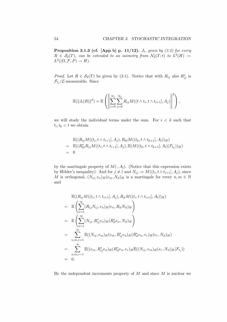
54 CHAPTER 3. STOCHASTIC INTEGRATION
Proposition 3.1.3 (cf. [App b] p. 11/12). Jt, given by (3.2) for everyR ∈ S2(T ), can be extended to an isometry from N2(T ; t) to L2(H) :=L2((Ω,F , P ) → H).
Proof. Let R ∈ S2(T ) be given by (3.1). Notice that with Rij also R∗ij is
Fti/L-measurable. Since
E(‖Jt(R)‖2) = E
∥∥∥∥∥∥N1∑i=0
N2∑j=0
RijM((t ∧ ti, t ∧ ti+1], Aj)
∥∥∥∥∥∥2 ,
we will study the individual terms under the sum. For i < k such thatti, tk < t we obtain
E((RijM((ti, t ∧ ti+1], Aj), RklM((tk, t ∧ tk+1], Al))H)= E((R∗
klRijM((ti, t ∧ ti+1], Aj),E(M((tk, t ∧ tk+1], Al)|Ftk))H)= 0
by the martingale property of M(·, Al). (Notice that this expression existsby Holder’s inequality). And for j 6= l and Nij := M((ti, t∧ ti+1], Aj), sinceM is orthogonal, (Nij , en)H(em, Nil)H is a martingale for every n,m ∈ Nand
E((RijM((ti, t ∧ ti+1], Aj), RilM((ti, t ∧ ti+1], Al))H)
= E
( ∞∑n=1
(RijNij , en)H(en, RilNil)H
)
= E
( ∞∑n=1
(Nij , R∗ijen)H(R∗
ilen, Nil)H
)
=∞∑
n,m,r=1
E((Nij , em)H(em, R∗ijen)H(R∗
ilen, er)H(er, Nil)H)
=∞∑
n,m,r=1
E((em, R∗ijen)H(R∗
ilen, er)HE((Nij , em)H(er, Nil)H |Fti))
= 0.
By the independent increments property of M and since M is nuclear we

3.1. STRONG STOCHASTIC INTEGRALS 55
have
E(‖RijM((ti, t ∧ ti+1], Aj)‖2)
=∞∑
n,m,r=1
E((em, R∗ijen)H(R∗
ijen, er)H)E((Nij , em)H(er, Nij)H)
=∞∑
n,m,r=1
E((em, R∗ijen)H(R∗
ijen, er)H)(er, TAjem)H%((ti, t ∧ ti+1])
=∞∑
m=1
E((Rijem, RijTAjem)H)%((ti, t ∧ ti+1])
= E(tr(R∗ijRijTAj ))%((ti, t ∧ ti+1]).
Moreover, for every A ∈ A and some operator S ∈ L(H)
tr(STA) =∞∑
n=1
(en, STAen)H =∞∑
n=1
(S∗en,
∫ATxenν(dx)
)H
=∫
Atr(STx)ν(dx).
Using these calculations we find
E(‖Jt(R)‖2) = E
∥∥∥∥∥∥N1∑i=0
N2∑j=0
RijM((t ∧ ti, t ∧ ti+1], Aj)
∥∥∥∥∥∥2
=N1∑i=0
N2∑j=0
E(‖RijM((t ∧ ti, t ∧ ti+1], Aj)‖2)
=N1∑i=0
N2∑j=0
E(tr(R∗ijRijTAj ))%((t ∧ ti, t ∧ ti+1])
=N1∑i=0
N2∑j=0
E
(∫Aj
tr(R∗ijRijTx)ν(dx)
)%((t ∧ ti, t ∧ ti+1])
= E
(∫ T
0
∫S‖1(0,t](s)R(s, x)
√Tx‖2
2ν(dx)%(ds)
)= ‖R|(0,t]×Ω×S‖2
N2(T ;t).
Now let R ∈ N2(T ). Then R can be approximated in N2(T ) by a sequenceRn ⊂ S2(T ). Hence
limn,m→∞
E(‖Jt(Rn)− Jt(Rm)‖2) = limn,m→∞
‖(Rn −Rm)|(0,t]×Ω×S‖2N2(T ;t) = 0,
and therefore Jt(Rn) is a Cauchy sequence in L2(H). Now we can defineJt(R) as the limit of Jt(Rn) in L2(H).

56 CHAPTER 3. STOCHASTIC INTEGRATION
Now for any R ∈ N2(T ) = N2(T ; T ) the strong stochastic integral of Rwith respect to the orthogonal and nuclear martingale measure M is definedas ∫ t
0
∫SR(s, x)M(ds, dx) := Jt(R)
for any 0 ≤ t ≤ T .
Remark 3.1.4. A sufficient condition for R with (s, ω, x) 7→ R(s, ω, x)y isP ⊗ Σ-measurable for every y ∈ H to be in N2(T ) is
‖R‖N2(T ) = E
(∫ T
0
∫S
∥∥∥R(s, x)√Tx
∥∥∥2
2ν(dx)%(ds)
) 12
≤ E
(∫ T
0
∫S‖R(s, x)‖2 tr(Tx)ν(dx)%(ds)
) 12
<∞.
Theorem 3.1.5. The process (∫ t0
∫S R(s, x)M(ds, dx), t ≥ 0) is an H-valued
strongly cadlag square-integrable martingale. Furthermore
E
(∥∥∥∥∫ t
0
∫SR(s, x)M(ds, dx)
∥∥∥∥2)
(3.3)
= E
(∫ T
0
∫S
1(0,t](s)R(s, x)√Tx‖2
2ν(dx)%(ds)
).
Proof. Let R ∈ S2(T ) be given by (3.1). For s ≤ t set i0 := maxi; ti ≤ s.Without loss of generality we can assume that tN1 < t and have
E(∫ t
0
∫SR(s, x)M(ds, dx)
∣∣∣∣Fs
)=
N1∑i=0
N2∑j=0
E(RijM((ti, t ∧ ti+1], Aj)|Fs)
=N1∑i=0
N2∑j=0
∞∑n=1
E((M((ti, t ∧ ti+1], Aj), R∗ijen)Hen|Fs)
=N1∑i=0
N2∑j=0
∞∑n=1
E((M((ti, t ∧ ti+1], Aj), R∗ijen)H |Fs)en
=N2∑j=0
i0−1∑i=0
∞∑n=1
(M((ti, ti+1], Aj), R∗ijen)Hen
+N2∑j=0
∞∑n=1
(E(M((ti0 , t ∧ ti0+1], Aj)|Fs), R∗i0jen)Hen

3.2. WEAK STOCHASTIC INTEGRALS 57
+N2∑j=0
N1∑i=i0+1
∞∑n=1
E((E(M((ti, t ∧ ti+1], Aj)|Fti), R∗ijen)H |Fs)en
=N2∑j=0
(i0−1∑i=0
RijM((ti, ti+1], Aj) +Ri0jM((ti0 , s], Aj)
)
=∫ s
0
∫S(F (s, x),M(ds, dx))H .
Now the result can be extended to any R ∈ N2(T ): R can be written as thelimit of some Rn ⊂ S2(T ) in N2(T ). Then the corresponding integral canby Prop. 3.1.3 be written as a limes of martingales in L2(H), hence it isalso a martingale. Again by Proposition 3 in [Kun] every square-integrablemartingale is strongly cadlag P -a.s..
3.2 Weak Stochastic Integrals
Apart from the strong stochastic integral another (real-valued) stochasticintegral can be constructed. The weak stochastic integral of an H-valuedfunction F with respect to M will be written as∫ t
0
∫S(F (s, x),M(ds, dx))H .
Remark 3.2.1. Alternatively to the construction which we will give in thissection, the weak stochastic integral can also be obtained as a special caseof the strong stochastic integral. In the last section we have constructed thestrong stochastic integral for integrands R for which R(s, ω, x) is a linearoperator from H into the same space. If the construction is generalizedto integrands for which R(s, ω, x) is a linear operator from H to anotherHilbert space H then in particular, one can choose H = R. Hence bythe Riesz isomorphism one can construct a stochastic integral for H-valuedfunctions which takes values in R. For such a function F : [0, T ]×Ω×S → Hwe can identify F (s, ω, x) ∈ H with the operator SF (s,ω,x) defined by
SF (s,ω,x)y = (F (s, ω, x), y)H
for any y ∈ H. Let L2(H,R) denote the space of all Hilbert-Schmidt opera-tors from H to R and ‖ · ‖L2(H,R) the corresponding Hilbert-Schmidt norm.Then for an orthonormal basis ek of H we have
‖SF (s,ω,x)
√Tx‖2
L2(H,R) =∞∑
k=1
∣∣∣(F (s, ω, x),√Txek)H
∣∣∣2=
∞∑k=1
∣∣∣(√TxF (s, ω, x), ek)H
∣∣∣2 = ‖√TxF (s, ω, x)‖2.
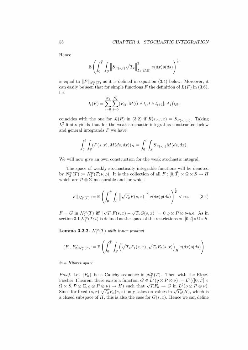
58 CHAPTER 3. STOCHASTIC INTEGRATION
Hence
E
(∫ T
0
∫S
∥∥∥SF (s,x)
√Tx
∥∥∥2
L2(H,R)ν(dx)%(ds)
) 12
is equal to ‖F‖Nw2 (T ) as it is defined in equation (3.4) below. Moreover, it
can easily be seen that for simple functions F the definition of It(F ) in (3.6),i.e.
It(F ) =N1∑i=0
N2∑j=0
(Fij ,M((t ∧ ti, t ∧ ti+1], Aj))H ,
coincides with the one for Jt(R) in (3.2) if R(s, ω, x) = SF (s,ω,x). TakingL2-limits yields that for the weak stochastic integral as constructed belowand general integrands F we have
∫ t
0
∫S(F (s, x),M(ds, dx))H =
∫ t
0
∫SSF (s,x)M(ds, dx).
We will now give an own construction for the weak stochastic integral.
The space of weakly stochastically integrable functions will be denotedby Nw
2 (T ) := Nw2 (T ; ν, %). It is the collection of all F : [0, T ]× Ω× S → H
which are P ⊗ Σ-measurable and for which
‖F‖Nw2 (T ) := E
(∫ T
0
∫S
∥∥∥√TxF (s, x)∥∥∥2ν(dx)%(ds)
) 12
<∞. (3.4)
F = G in Nw2 (T ) iff ‖
√TxF (s, x) −
√TxG(s, x)‖ = 0 % ⊗ P ⊗ ν-a.e. As in
section 3.1Nw2 (T ; t) is defined as the space of the restrictions on [0, t]×Ω×S.
Lemma 3.2.2. Nw2 (T ) with inner product
(F1, F2)Nw2 (T ) := E
(∫ T
0
∫S
(√TxF1(s, x),
√TxF2(s, x)
)Hν(dx)%(ds)
)
is a Hilbert space.
Proof. Let Fn be a Cauchy sequence in Nw2 (T ). Then with the Riesz-
Fischer Theorem there exists a function G ∈ L2(%⊗ P ⊗ ν) := L2(([0, T ]×Ω × S,P ⊗ Σ, % ⊗ P ⊗ ν) → H) such that
√T·Fn → G in L2(% ⊗ P ⊗ ν).
Since for fixed (s, x)√TxFn(s, x) only takes on values in
√Tx(H), which is
a closed subspace of H, this is also the case for G(s, x). Hence we can define

3.2. WEAK STOCHASTIC INTEGRALS 59
F (s, x) :=√Tx
−1G(s, x). But then
E
(∫ T
0
∫S
∥∥∥√Tx(Fn(s, x)− F (s, x))∥∥∥2ν(dx)%(ds)
)
= E
(∫ T
0
∫S
∥∥∥√TxFn(s, x)−√Tx
√Tx
−1G(s, x)
∥∥∥2ν(dx)%(ds)
)
= E
(∫ T
0
∫S
∥∥∥√TxFn(s, x)−G(s, x)∥∥∥2ν(dx)%(ds)
).
Hence Fn → F in Nw2 (T ).
As before the construction of the stochastic integral will be done forsimple functions first. As Sw
2 (T ) define the subspace of all F ∈ Nw2 (T )
which are of the form
F =N1∑i=0
N2∑j=0
Fij1(ti,ti+1]1Aj (3.5)
with N1, N2 ∈ N, 0 = t0 < t1 < · · · < tN1+1 = T , each Fij being a boundedFti-measurable random variable and A0, . . . , AN2+1 ∈ A disjoint.
Lemma 3.2.3. The subspace Sw2 (T ) is dense in Nw
2 (T ).
Proof. The proof can be given along the lines of the proof of Lemma 3.1.2.Let en be an orthonormal basis of H. For some k ∈ N define G(s, ω, x) :=ek1B(s)1C(ω)1A(x) where B = (t1, t2] with t1, t2 ∈ [0, T ], A ∈ A and C ∈Fti . Choose some F ∈ (Sw
2 (T ))⊥. Then
0 = (F,G)Nw2 (T )
= E
(∫ T
0
∫S
(√TxF (s, x),
√TxG(s, x)
)Hν(dx)%(ds)
)
= E(
1C
∫B
∫A(TxF (s, x), ek)Hν(dx)%(ds)
).
Again
µ(G) :=∫
G(TxF (s, x), ek)Hd(%⊗ P ⊗ ν), G ∈ P ⊗ Σ
defines a signed measure on P ⊗Σ. As in Lemma 3.1.2 (TxF (s, x), ek)H = 0for all k ∈ N %⊗ P ⊗ ν-a.s. Then
‖F‖2Nw
2 (T ) = E
(∫ T
0
∫S(TxF (s, x), F (s, x))Hν(dx)%(ds)
)
= E
(∫ T
0
∫S
∞∑k=1
(TxF (s, x), ek)H(ek, F (s, x))Hν(dx)%(ds)
)= 0,
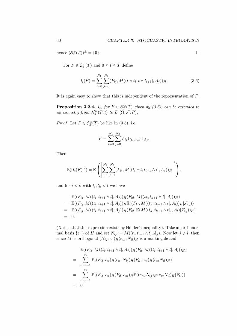
60 CHAPTER 3. STOCHASTIC INTEGRATION
hence (Sw2 (T ))⊥ = 0.
For F ∈ Sw2 (T ) and 0 ≤ t ≤ T define
It(F ) =N1∑i=0
N2∑j=0
(Fij ,M((t ∧ ti, t ∧ ti+1], Aj))H . (3.6)
It is again easy to show that this is independent of the representation of F .
Proposition 3.2.4. It, for F ∈ Sw2 (T ) given by (3.6), can be extended to
an isometry from Nw2 (T ; t) to L2(Ω,F , P ).
Proof. Let F ∈ Sw2 (T ) be like in (3.5), i.e.
F =N1∑i=0
N2∑j=0
Fij1(ti,ti+1]1Aj .
Then
E(|It(F )|2) = E
∣∣∣∣∣∣N1∑i=1
N2∑j=1
(Fij ,M((ti ∧ t, ti+1 ∧ t], Aj))H
∣∣∣∣∣∣2 ,
and for i < k with ti, tk < t we have
E((Fij ,M((ti, ti+1 ∧ t], Aj))H(Fkl,M((tk, tk+1 ∧ t], Al))H)= E((Fij ,M((ti, ti+1 ∧ t], Aj))HE((Fkl,M((tk, tk+1 ∧ t], Al))H |Ftk))= E((Fij ,M((ti, ti+1 ∧ t], Aj))H(Fkl,E(M((tk, tk+1 ∧ t], , Al)|Ftk))H)= 0.
(Notice that this expression exists by Holder’s inequality). Take an orthonor-mal basis en of H and set Nij := M((ti, ti+1 ∧ t], Aj). Now let j 6= l, thensince M is orthogonal (Nij , en)H(em, Nil)H is a martingale and
E((Fij ,M((ti, ti+1 ∧ t], Aj))H(Fil,M((ti, ti+1 ∧ t], Al))H)
=∞∑
n,m=1
E((Fij , en)H(en, Nij)H(Fil, em)H(emNil)H)
=∞∑
n,m=1
E((Fij , en)H(Fil, em)HE((en, Nij)H(emNil)H |Fti))
= 0.

3.2. WEAK STOCHASTIC INTEGRALS 61
Since M has independent increments
E(|(Fij ,M((ti, ti+1 ∧ t], Aj))H |2)
=∞∑
n,m=1
E((Fij , en)H(Fij , em)H)E((en, Nij)H(emNij)H)
=∞∑
n,m=1
E((Fij , en)H(Fij , em)H)(en, TAjem)H%((ti, ti+1 ∧ t])
=∞∑
m=1
E((Fij , TAjem)H(Fij , em)H)%((ti, ti+1 ∧ t])
= E((TAjFij , Fij)H)%((ti, ti+1 ∧ t])
= E
(∫Aj
(TxFij , Fij)Hν(dx)
)%((ti, ti+1 ∧ t]).
Hence with the calculations from above
E(|It(F )|2)
= E
∣∣∣∣∣∣N1∑i=1
N2∑j=1
(Fij ,M((ti ∧ t, ti+1 ∧ t], Aj))H
∣∣∣∣∣∣2
=N1∑i=1
N2∑j=1
E(|(Fij ,M((ti ∧ t, ti+1 ∧ t], Aj))H |2
)
=N1∑i=1
N2∑j=1
E
(∫Aj
(TxFij , Fij)Hν(dx)
)%((ti ∧ t, ti+1 ∧ t])
= E
(∫ T
0
∫S
∥∥∥1(0,t](s)√TxF (s, x)
∥∥∥2ν(dx)%(ds)
)= ‖F|(0,t]×Ω×S‖2
Nw2 (T ;t).
But then for arbitrary F ∈ Nw2 (T ) there exists a sequence Fn ⊂ Sw
2 (T )which converges to F in Nw
2 (T ) and
limn,m→∞
E(|It(Fn)− It(Fm)|2) = limn,m→∞
‖(Fn − Fm)|(0,t]×Ω×S‖2Nw
2 (T ;t) = 0.
So we can define It(F ) to be the limit of It(Fn) in L2(Ω,F , P ) and of coursethe equality still holds.
Let F ∈ Nw2 (T ). Then define the weak stochastic integral of F with
respect to the orthogonal martingale measure M as∫ t
0
∫S(F (s, x),M(ds, dx))H := It(F ). (3.7)

62 CHAPTER 3. STOCHASTIC INTEGRATION
Proposition 3.2.5. Let F ∈ Nw2 (T ). Then (
∫ t0
∫S(F (s, x),M(ds, dx))H ,
t ≥ 0) is a centered square-integrable martingale.
Proof. First let F ∈ Sw2 (T ) be like in (3.5). Let s ≤ t and set i0 :=
maxi; ti ≤ s. Without loss of generality assume tN1 < t. Then
E(∫ t
0
∫S(F (s, x),M(ds, dx))H
∣∣∣∣Fs
)=
N1∑i=0
N2∑j=0
E((Fij ,M((ti, t ∧ ti+1], Aj))H |Fs)
=N2∑j=0
i0−1∑i=0
(Fij ,M((ti, ti+1], Aj))H
+N2∑j=0
(Fi0j ,E(M((ti0 , t ∧ ti0+1], Aj)|Fs))H
+N2∑j=0
N1∑i=i0+1
E((Fij ,E(M((ti, t ∧ ti+1], Aj)|Fti))H |Fs)
=N2∑j=0
(i0−1∑i=0
(Fij ,M((ti, ti+1], Aj))H + (Fi0j ,M((ti0 , s], Aj))H
)
=∫ s
0
∫S(F (s, x),M(ds, dx))H .
Now if F ∈ Nw2 (T ) then it can be approximated by a sequence Fn ⊂
Sw2 (T ) in Nw
2 (T ). Then by Proposition 3.2.4 the weak stochastic inte-gral
∫ t0
∫S(F (s, x),M(ds, dx))H can be approximated by the weak integrals∫ t
0
∫S(Fn(s, x),M(ds, dx))H in L2(Ω,F , P ). Hence it is also a martingale. It
is obvious that this martingale is centered and square-integrable.
3.3 Properties of the Stochastic Integral
In this section we will show some useful properties of the weak and thestrong stochastic integral which were constructed above.
Proposition 3.3.1 (cf. [App b] Theorem 3). Let C ∈ L(H) and R ∈N2(T ). Then CR ∈ N2(T ) and for every 0 ≤ t ≤ T
C
∫ t
0
∫SR(s, x)M(ds, dx) =
∫ t
0
∫SCR(s, x)M(ds, dx) P -a.s..

3.3. PROPERTIES OF THE STOCHASTIC INTEGRAL 63
Proof. CR ∈ N2(T ) since
E
(∫ T
0
∫S‖CR(t, x)
√Tx‖2
2ν(dx)%(dt)
) 12
≤ E
(∫ T
0
∫S‖C‖2‖R(t, x)
√Tx‖2
2ν(dx)%(dt)
) 12
= ‖C‖‖R‖N2(T ).
Moreover, for R ∈ S2(T ) like in (3.1) we have
C
∫ t
0
∫SR(s, x)M(ds, dx) = C
N1∑i=0
N2∑j=0
RijM((t ∧ ti, t ∧ ti+1], Aj)
=∫ t
0
∫SCR(s, x)M(ds, dx).
Now let Rn ⊂ S2(T ) with Rn → R in N2(T ). Then by Proposition 3.1.3
E
(∫ T
0
∫S‖1(0,t](s)C(R(s, x)−Rn(s, x))
√Tx‖2
2ν(dx)%(dt)
)
≤ ‖C‖2E
(∫ T
0
∫S‖1(0,t](s)(R(s, x)−Rn(s, x))
√Tx‖2
2ν(dx)%(dt)
),
and by definition the sequence of the integrals∫ t0
∫S CRn(s, x)M(ds, dx)
converges to∫ t0
∫S CR(s, x)M(ds, dx) in L2(H). Also
E
(∥∥∥∥C ∫ t
0
∫S(Rn(s, x)−R(s, x))M(ds, dx)
∥∥∥∥2)
≤ ‖C‖2E
(∫ T
0
∫S‖1(0,t](s)(Rn(s, x)−R(s, x))
√Tx‖2
2ν(dx)%(dt)
).
Hence
E
(∥∥∥∥∫ t
0
∫SCR(s, x)M(ds, dx)− C
∫ t
0
∫SR(s, x)M(ds, dx)
∥∥∥∥2) 1
2
≤ limn→∞
E
(∥∥∥∥∫ t
0
∫SC(R(s, x)−Rn(s, x))M(ds, dx)
∥∥∥∥2) 1
2
+ limn→∞
E
(∥∥∥∥C ∫ t
0
∫S(Rn(s, x)−R(s, x))M(ds, dx)
∥∥∥∥2) 1
2
= 0.

64 CHAPTER 3. STOCHASTIC INTEGRATION
Proposition 3.3.2 (Compatibility of weak and strong integration;cf. Thm. 4 in [App b]). Let R ∈ N2(T ). Then R∗y ∈ Nw
2 (T ) for everyy ∈ H and for each 0 ≤ t ≤ T(
y,
∫ t
0
∫SR(s, x)M(ds, dx)
)H
=∫ t
0
∫S(R(s, x)∗y,M(ds, dx))H (3.8)
P -a.s..
Proof. Let R ∈ N2(T ) and y ∈ H, then
‖R∗y‖2Nw
2 (T )
= E
(∫ T
0
∫S
∥∥∥√TxR(s, x)∗y∥∥∥2ν(dx)%(ds)
)
≤ ‖y‖2E
(∫ T
0
∫S
∥∥∥√TxR(s, x)∗∥∥∥2ν(dx)%(ds)
)
≤ ‖y‖2E
(∫ T
0
∫S
∥∥∥R(s, x)√Tx
∥∥∥2
2ν(dx)%(ds)
)= ‖y‖2‖R‖2
N2(T ) <∞.
Hence both integrals exist. Now (3.8) can be shown for every R ∈ S2(T ):(y,
∫ t
0
∫SR(s, x)M(ds, dx)
)H
=N1∑i=0
N2∑j=0
(y,RijM((t ∧ ti, t ∧ ti+1], Aj))H
=N1∑i=0
N2∑j=0
(R∗ijy,M((t ∧ ti, t ∧ ti+1], Aj))H
=∫ t
0
∫S(R(s, x)∗y,M(ds, dx))H .
But for R ∈ N2(T ) there can be chosen a sequence Rn ⊂ S2(T ) withRn → R in N2(T ). Obviously R∗
ny ⊂ Sw2 (T ). Then for
It(R∗y) =∫ t
0
∫S(R(s, x)∗y,M(ds, dx))H
and
Jt(R) =∫ t
0
∫SR(s, x)M(ds, dx),

3.3. PROPERTIES OF THE STOCHASTIC INTEGRAL 65
we have
E(|(y, Jt(R))H − It(R∗y)|2
) 12
≤ limn→∞
(E(|(y, Jt(R)− Jt(Rn))H |
2) 1
2 + E(|It(R∗
ny)− It(R∗y)|2) 1
2
)≤ ‖y‖ lim
n→∞E(‖Jt(R)− Jt(Rn)‖2
) 12 + lim
n→∞‖R∗y −R∗
ny‖Nw2 (T )
≤ 2‖y‖ limn→∞
‖R−Rn‖N2(T ) = 0.
Remark 3.3.3. Using a slightly generalized version of Prop. 3.3.1 and withthe notations from Remark 3.2.1 we can give an alternative proof:(
y,
∫ t
0
∫SR(s, x)M(ds, dx)
)H
= Sy
(∫ t
0
∫SR(s, x)M(ds, dx)
)=
∫ t
0
∫SSyR(s, x)M(ds, dx) =
∫ t
0
∫SSR(s,x)∗yM(ds, dx)
=∫ t
0
∫S(R(s, x)∗y,M(ds, dx))H .
Now a useful stochastic version of the Fubini theorem will be shown.Introduce a measure space (W,W, µ) with µ finite. By G2(W ) denote thespace of all operator valued mappings R on [0, T ] × Ω × S ×W such that(s, ω, x, w) 7→ R(s, ω, x, w)y is P ⊗ Σ⊗W-measurable for each y ∈ H and
‖R‖G2(W ) :=
[E
(∫W
∫ T
0
∫S‖R(s, x, w)
√Tx‖2
2ν(dx)%(ds)µ(dw)
)] 12
<∞.
Again two mappings are identified in G2(W ) if they are equal %⊗P ⊗ ν⊗µ-a.e..
Theorem 3.3.4 (Stochastic Fubini). Let R ∈ G2(W ). Then for each0 ≤ t ≤ T ∫
W
(∫ t
0
∫SR(s, x, w)M(ds, dx)
)µ(dw)
=∫ t
0
∫S
(∫WR(s, x, w)µ(dw)
)M(ds, dx)
where the left hand side is meant as an L2(H)-valued Bochner integral.
Proof. Note that by Jensen’s inequality∥∥∥∥∫WR(s, x, w)µ(W )−1µ(dw)
∥∥∥∥2
≤∫
W‖R(s, x, w)‖2µ(W )−1µ(dw).
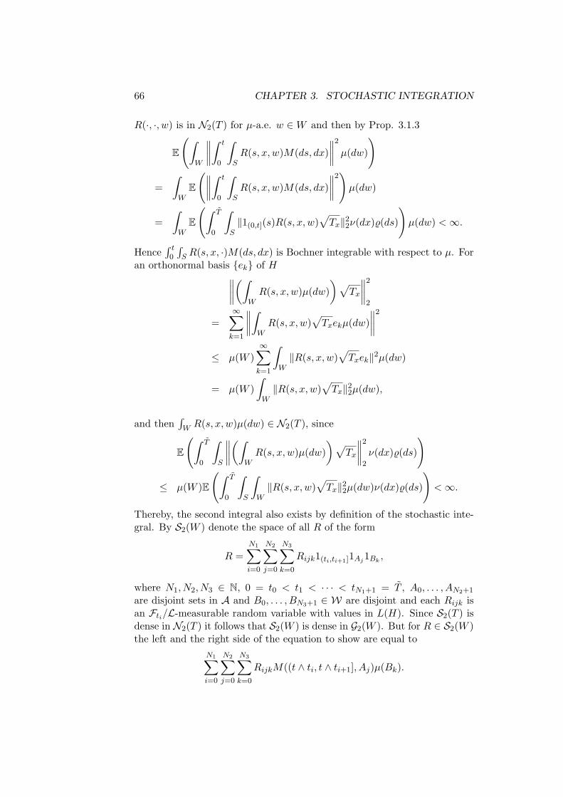
66 CHAPTER 3. STOCHASTIC INTEGRATION
R(·, ·, w) is in N2(T ) for µ-a.e. w ∈W and then by Prop. 3.1.3
E
(∫W
∥∥∥∥∫ t
0
∫SR(s, x, w)M(ds, dx)
∥∥∥∥2
µ(dw)
)
=∫
WE
(∥∥∥∥∫ t
0
∫SR(s, x, w)M(ds, dx)
∥∥∥∥2)µ(dw)
=∫
WE
(∫ T
0
∫S‖1(0,t](s)R(s, x, w)
√Tx‖2
2ν(dx)%(ds)
)µ(dw) <∞.
Hence∫ t0
∫S R(s, x, ·)M(ds, dx) is Bochner integrable with respect to µ. For
an orthonormal basis ek of H∥∥∥∥(∫WR(s, x, w)µ(dw)
)√Tx
∥∥∥∥2
2
=∞∑
k=1
∥∥∥∥∫WR(s, x, w)
√Txekµ(dw)
∥∥∥∥2
≤ µ(W )∞∑
k=1
∫W‖R(s, x, w)
√Txek‖2µ(dw)
= µ(W )∫
W‖R(s, x, w)
√Tx‖2
2µ(dw),
and then∫W R(s, x, w)µ(dw) ∈ N2(T ), since
E
(∫ T
0
∫S
∥∥∥∥(∫WR(s, x, w)µ(dw)
)√Tx
∥∥∥∥2
2
ν(dx)%(ds)
)
≤ µ(W )E
(∫ T
0
∫S
∫W‖R(s, x, w)
√Tx‖2
2µ(dw)ν(dx)%(ds)
)<∞.
Thereby, the second integral also exists by definition of the stochastic inte-gral. By S2(W ) denote the space of all R of the form
R =N1∑i=0
N2∑j=0
N3∑k=0
Rijk1(ti,ti+1]1Aj1Bk,
where N1, N2, N3 ∈ N, 0 = t0 < t1 < · · · < tN1+1 = T , A0, . . . , AN2+1
are disjoint sets in A and B0, . . . , BN3+1 ∈ W are disjoint and each Rijk isan Fti/L-measurable random variable with values in L(H). Since S2(T ) isdense in N2(T ) it follows that S2(W ) is dense in G2(W ). But for R ∈ S2(W )the left and the right side of the equation to show are equal to
N1∑i=0
N2∑j=0
N3∑k=0
RijkM((t ∧ ti, t ∧ ti+1], Aj)µ(Bk).
3.3. PROPERTIES OF THE STOCHASTIC INTEGRAL 67
If R ∈ G2(W ) is arbitrary, it can be approximated by a sequence Rn ⊂S2(W ). But then
E
(∥∥∥∥∫W
(∫ t
0
∫S(R(s, x, w)−Rn(s, x, w))M(ds, dx)
)µ(dw)
∥∥∥∥2)
≤ µ(W )‖R−Rn‖2G2(W ) → 0
for n→∞ and
E
(∥∥∥∥∫ t
0
∫S
(∫W
(R(s, x, w)−Rn(s, x, w))µ(dw))M(ds, dx)
∥∥∥∥2)
≤ µ(W )‖R−Rn‖2G2(W ) → 0
for n→∞.
68 CHAPTER 3. STOCHASTIC INTEGRATION

Chapter 4
Stochastic Equations withLevy Noise
Now we apply the developed integration theory from the last chapter andconsider stochastic partial differential equations driven by a Levy process.If (S(t), t ≥ 0) is a C0-semigroup (S(t), t ≥ 0) with generator J and Ca bounded linear operator acting on H then we can define the stochasticconvolution
XJ,C(t) :=∫ t
0S(t− s)CdX(s)
for any H-valued Levy process X (see section 4.1). In the subsequent section4.2 we will find a weak solution to the following Ornstein-Uhlenbeck typestochastic differential equation
dY (t) = (JY (t) + f(t))dt+ CdX(t)Y (0) = Y0.
Here f is an adapted process and Y0 some initial value. In [DaPrZa] existenceand uniqueness is shown for the case where X is a Brownian motion withdrift. [App b] has generalized the result (in the case f ≡ 0) to Levy processeswith similar methods. We show existence of a weak solution following theapproach of [DaPrZa]. The compatibility of weak and strong integration aswell as the stochastic Fubini theorem, which were shown before, are veryuseful tools.
In section 4.3 a non-linear drift term is added to the Ornstein-Uhlenbeckequation. For a function F : H → H fulfilling a Lipschitz condition we havethe equation
dY (t) = (JY (t) + F (Y (t)))dt+ CdX(t)Y (0) = Y0.
The idea of section 4.3 is to prove existence and uniqueness of a weak solutionby a fixed point argument as in Chapter 7 of [DaPrZa]. However, this is not
69

70 CHAPTER 4. STOCHASTIC EQUATIONS WITH LEVY NOISE
straightforward. Since for a Levy process first and second moments may notexist we have to impose an additional condition on the jumps of the Levyprocess X: For some ε > 0
sup0≤t≤T
‖∆X(t)‖ ∈ L2+ε(R) = L2+ε(Ω → R).
We find that a stochastic process Y is a weak solution of the consideredequation if and only if Y is a fixed point under the mapping Y 7→ ψ(Y ) with
ψ(Y )(t) =∫ t
0S(t− s)F (Y (s))ds+ S(t)Y0 +XJ,C(t)).
Existence and uniqueness is then proved by an application of Banach’s fixedpoint theorem on a suitable space. Different from [DaPrZa] we do not haveto put together the solution from solutions on single subintervals of [0, T ] byusing a weighted norm on the corresponding Banach space, as in [Kno b].
Assumption 4.0.1. In the whole chapter we take the following objects andproperties as given:
• Let X be a Levy process with Levy Ito decomposition (2.7) and forsome ε > 0
sup0≤t≤T
‖∆X(t)‖ ∈ L2+ε(R) = L2+ε(Ω → R). (4.1)
• (S(t), t ≥ 0) shall be a C0-semigroup with infinitesimal generator J .
• C ∈ L(H).
• f : [0, T ] → L2(H) = L2(Ω → H) a stochastic process, adapted to(Ft; t ≥ 0) which is (as L2(H)-valued function) Bochner integrable on[0, T ].
• Y0 ∈ L2(H) = L2(Ω → H) and F0-measurable.
Remark 4.0.2. Let N = (N(t), t ≥ 0) be a real-valued Poisson process withintensity c > 0. Then for any 1 ≤ p < ∞ we have N(t) ∈ Lp(R) for t ≥ 0and t 7→ N(t) is continuous in Lp(R): Since for n ∈ N with n ≥ p
E(|N(t)−N(s)|p) ≤ E(|N(t)−N(s)|n)
it is sufficient to consider p = n ∈ N. But the moment generating functionof a random variable Y which is Poisson distributed with parameter α > 0is
ϕα(t) = E(etY)
=∞∑
k=0
e−ααketk
k!= exp(α(et − 1)).
4.1. THE STOCHASTIC CONVOLUTION 71
Since ϕα ∈ C∞(R) all moments E(Y n) = ϕ(n)α (0), n ∈ N exist. Moreover for
any n ∈ N the n-th derivative of ϕα is of the form
ϕ(n)α (t) = αgn(α, t)
where α 7→ gn(α, t) is continuous and therefore bounded in α on each com-pactum [−ε, ε]. Hence
limα→0
ϕ(n)α (0) = lim
α→0αgn(α, 0) = 0.
Now the continuity of N in Ln(R) for every n ∈ N follows, because
lims→t
E((N(t)−N(s))n) = lims→t
E((N(t− s))n) = lims→t
(t− s)gn(t− s, 0) = 0.
We obtain that by (4.1) X(t) ∈ L2(H) for any 0 ≤ t ≤ T : Let p > 1be given with 1/p + 1/(2 + ε) = 1/2. Then by the generalized Holder’sinequality
E
∥∥∥∥∥∥∑
0<s≤t
∆X(s)1‖x‖≥1(∆X(s))
∥∥∥∥∥∥2
12
≤ E
( sup0≤t≤T
‖∆X(t)‖
)2
N(t, ‖x‖ ≥ 1)2 1
2
≤ E
( sup0≤t≤T
‖∆X(t)‖
)2+ε 1
2+ε
E (N(t, ‖x‖ ≥ 1)p)1p
< ∞
since N(·, ‖x‖ ≥ 1) is a Poisson process and therefore in Lp(R). But themartingale part in the Levy Ito decomposition is in L2(H) by construction.Therefore we will treat X as a mapping X : [0, T ] → L2(H).
4.1 The Stochastic Convolution
First we will define the stochastic convolution. Some preparations on C0-semigroups are needed (compare [Paz] sections 1.1. and 1.2.):
A strongly continuous semigroup of bounded linear operators or a C0-semigroup is a one parameter family (S(t), t ≥ 0) of bounded linear operatorsS(t) ∈ L(H) with
• S(0) = Id, where Id is the identity operator on H,
• S(s+ t) = S(t)S(s) for every s, t ≥ 0 (semigroup property),

72 CHAPTER 4. STOCHASTIC EQUATIONS WITH LEVY NOISE
• limt↓0 S(t)x = x for every x ∈ H (strong continuity).
Lemma 4.1.1. Let (S(t), t ≥ 0) be a C0-semigroup. Then there exist con-stants β ≥ 0 and M ≥ 1 such that
‖S(t)‖ ≤Meβt for all t ≥ 0. (4.2)
Proof. (cf. [Paz] Ch. 1, Theorem 2.2.).
Lemma 4.1.2. If (S(t), t ≥ 0) is a C0-semigroup then for every x ∈ H,t 7→ S(t)x is a strongly continuous function from R+ into H.
Proof. (cf. [Paz] Ch. 1, Cor. 2.3.).
Define the infinitesimal generator of a C0-semigroup (S(t), t ≥ 0) as theoperator J with domain
D(J) =x ∈ H; lim
t↓0
S(t)x− x
texists
and
Jx = limt↓0
S(t)x− x
tfor all x ∈ D(J).
Proposition 4.1.3. Let (S(t), t ≥ 0) be a C0-semigroup with infinitesimalgenerator J . Then
• for every x ∈ H and t ≥ 0
limh→0
1h
∫ t+h
tS(s)xds = S(t)x,
• for every x ∈ H and t ≥ 0∫ t
0S(s)xds ∈ D(J)
and
J
(∫ t
0S(s)xds
)= S(t)x− x,
• for every x ∈ D(J) and t ≥ 0
S(t)x ∈ D(J)
andd
dtS(t)x = JS(t)x = S(t)Jx,

4.1. THE STOCHASTIC CONVOLUTION 73
• for every x ∈ D(J) and s, t ≥ 0
S(t)x− S(s)x =∫ t
sS(τ)Jxdτ =
∫ t
sJS(τ)xdτ.
Proof. (cf. [Paz] Ch. 1, Thm. 2.4.).
Proposition 4.1.4 (Properties of the infinitesimal generator). Theinfinitesimal generator J of a C0-semigroup (S(t), t ≥ 0) is densely defined,i.e. D(J) is dense in H, and J is a closed linear operator.
Proof. (cf. [Paz] Ch. 1, Cor. 2.5.).
Proposition 4.1.5 (The dual semigroup and its generator). Givena C0-semigroup (S(t), t ≥ 0) with infinitesimal generator J , (S(t)∗, t ≥ 0)is a C0-semigroup with infinitesimal generator J∗ which therefore is againdensely defined and closed.
Proof. (cf. [Paz] Ch. 1, Cor. 10.6.).
Proposition 4.1.6. Let (S(t), t ≥ 0) and (T (t), t ≥ 0) be C0-semigroupswith infinitesimal generators J and K respectively. If J = K then S(t) =T (t) for each t ≥ 0.
Proof. (cf. [Paz] Ch. 1, Thm. 2.6.).
Given the objects from Assumption 4.0.1 we are going to define thestochastic convolution XJ,C as
XJ,C(t) :=∫ t
0S(t− s)CdX(s) for every t ≥ 0. (4.3)
If XJ,C shall be well-defined we have to give sense to the stochastic integralin (4.3). By the Levy Ito decomposition (Theorem 2.4.7) the Levy processX can be written as
X(t) = tx0 +BQ(t) +∫‖x‖<1
xN(t, dx) +∫‖x‖≥1
xN(t, dx) (4.4)
Recall that here S = x ∈ H; ‖x‖ < 1, A0 = A ∈ B(S); 0 /∈ A andA = A0 ∪ A ∪ 0;A ∈ A0. We will define the stochastic integral in (4.3)by ∫ t
0S(t− s)CdX(s) :=
∫ t
0S(t− s)Cx0ds (4.5)
+∫ t
0S(t− s)CdBQ(s) (4.6)
+∫ t
0
∫‖x‖<1
S(t− s)CxN(ds, dx) (4.7)
+∫ t
0
∫‖x‖≥1
S(t− s)CxN(ds, dx), (4.8)

74 CHAPTER 4. STOCHASTIC EQUATIONS WITH LEVY NOISE
where the individual terms in (4.5), (4.6), (4.7) and (4.8) are defined asfollows:
We can define the integral in (4.5) as a Bochner integral. By (4.2) thisexists since∫ t
0‖S(t− s)Cx0‖ds ≤ ‖Cx0‖
∫ t
0‖S(t− s)‖ds
≤ ‖Cx0‖M∫ t
0eβ(t−s)ds <∞.
The integrators in (4.6) and (4.7) are Levy martingale measures like in(2.9). By Theorem 2.5.2 and Proposition 2.5.4 a Levy martingale measureis an orthogonal martingale measure with independent increments which isnuclear and decomposable. Hence one can construct the strong stochasticintegral with respect to such a Levy martingale measure. Set for A ∈ A
M1(t, A) = BQ(t)δ0(A)
andM2(t, A) =
∫A\0
xN(t, dx).
Now define∫ t
0S(t− s)CdBQ(s) :=
∫ t
0
∫‖x‖<1
S(t− s)CM1(ds, dx). (4.9)
Usually the stochastic integral with respect to a Brownian motion is defineddifferent from (4.9). See for example [DaPrZa], section 4.2., for the con-struction. We believe that for our class of integrands (i.e. the ones fromN2(T )) both integrals coincide. In any case in this text we will always usethe definition from (4.9). This is well defined since by Proposition 2.5.4(where ν = δ0, T0 = Q and % the Lebesgue measure on R+)
‖S(t− ·)C‖2N2(T ;t) =
∫ t
0
∫‖x‖<1
‖S(t− s)C√Tx‖2
2δ0(dx)ds
≤ tr(Q)∫ t
0‖S(t− s)C‖2ds
≤ ‖C‖2M2tr(Q)∫ t
0e2β(t−s)ds <∞.
By Lemma 4.1.2 t 7→ S(t)y is strongly continuous for every y ∈ H. Hencet 7→ S(t)y is P-measurable. So S(t− ·)C ∈ N2(T ; δ0, ds; t).
In the same way set∫ t
0
∫‖x‖<1
S(t− s)CxN(ds, dx) :=∫ t
0
∫‖x‖<1
S(t− s)CM2(ds, dx),

4.1. THE STOCHASTIC CONVOLUTION 75
where, with ν = λ, Tx = (x, ·)Hx and % the Lebesgue measure on R+,
‖S(t− ·)C‖2N2(T ;t) =
∫ t
0
∫‖x‖<1
‖S(t− s)C√Tx‖2
2λ(dx)ds
≤∫ t
0
∫‖x‖<1
‖S(t− s)C‖2‖x‖2λ(dx)ds
≤ ‖C‖2M2
∫ t
0e2β(t−s)
∫‖x‖<1
‖x‖2λ(dx)ds <∞,
hence S(t− ·)C ∈ N2(T ;λ, ds; t).Finally, the term in (4.8) will be defined as a random sum:
∫ t
0
∫‖x‖≥1
S(t− s)CxN(ds, dx)
:=∑
0<s≤t
S(t− s)C∆X(s)1‖x‖≥1(∆X(s)).
This is in L2(H) since
E
∥∥∥∥∥∥∑
0<s≤t
S(t− s)C∆X(s)1‖x‖≥1(∆X(s))
∥∥∥∥∥∥2
≤ M2e2βT ‖C‖2E
( sup0≤t≤T
‖∆X(t)‖
)2
N(t, ‖x‖ ≥ 1)2
< ∞.
Theorem 4.1.7 (cf. [App b] Thm. 6). For a Levy process X, C ∈L(H) and (S(t), t ≥ 0) a C0-semigroup with infinitesimal generator J thestochastic convolution XJ,C : [0, T ] → L2(H) given by
XJ,C(t) :=∫ t
0S(t− s)CdX(s) for every t ≥ 0
exists. Furthermore under Assumption 4.0.1 t 7→ XJ,C(t) is (as an L2(H)-valued mapping) continuous.
Proof. The existence follows from the construction above. We will investi-gate the continuity for the individual integrals from equations (4.5) to (4.8).First the continuity of t 7→
∫ t0 S(t − s)Cx0ds is obvious since this is con-
tinuous as an H-valued Bochner integral. Consider t 7→∫ t0
∫‖x‖≥1 S(t −

76 CHAPTER 4. STOCHASTIC EQUATIONS WITH LEVY NOISE
s)CxN(ds, dx). We have
E
(∥∥∥∥∥∫ t
0
∫‖x‖≥1
S(t− r)CxN(dr, dx)
−∫ s
0
∫‖x‖≥1
S(s− r)CxN(dr, dx)
∥∥∥∥∥2 1
2
≤ E
∥∥∥∥∥∥∑
0<r≤t
(S(t− r)− S(s− r ∧ s))C∆X(r)1‖x‖≥1(∆X(r))
∥∥∥∥∥∥2
12
+E
∥∥∥∥∥∥∑
t∧s<r≤t∨s
S(s− r ∧ s)C∆X(r)1‖x‖≥1(∆X(r))
∥∥∥∥∥∥2
12
.
But t 7→ S(t)y is strongly continuous for any y ∈ H and∥∥∥∥∥∥∑
0<r≤t
(S(t− r)− S(s− r ∧ s))C∆X(r)1‖x‖≥1(∆X(r))
∥∥∥∥∥∥≤ 2MeβT ‖C‖ sup
0≤t≤T
‖∆X(t)‖ (N(t, ‖x‖ ≥ 1)) ∈ L2(R)
which can be seen as in Remark 4.0.2 by the generalized Holder’s inequality(sup0≤t≤T ‖∆X(t)‖ ∈ L2+ε(R)). Hence we can apply Lebesgue’s dominatedconvergence theorem and obtain that the first summand vanishes for s→ t.The second summand can be estimated by
MeβT ‖C‖E
( sup0≤t≤T
‖∆X(t)‖
)2+ε 1
2+ε
E((N(t ∨ s, ‖x‖ ≥ 1)−N(t ∧ s, ‖x‖ ≥ 1))p)1p
for p with 1/p + 1/(2 + ε) = 1/2. But the Poisson process N(·, ‖x‖ ≥ 1)is (as an Lp(R)-valued mapping) continuous.
Set
M(t, A) = BQ(t)δ0(A) +∫
A\0xN(t, dx)
for any A ∈ A. We will show the continuity of t 7→∫ t0
∫‖x‖<1 S(t −
4.1. THE STOCHASTIC CONVOLUTION 77
r)CM(dr, dx) in L2(H). For 0 ≤ s, t ≤ T and ν = λ+ δ0 we have
E
(∥∥∥∥∥∫ t
0
∫‖x‖<1
S(t− r)CM(dr, dx)
−∫ s
0
∫‖x‖<1
S(s− r)CM(dr, dx)
∥∥∥∥∥2 1
2
≤ E
∥∥∥∥∥∫ t
0
∫‖x‖<1
(S(t− r)− S(s− r ∧ s))CM(dr, dx)
∥∥∥∥∥2 1
2
+E
∥∥∥∥∥∫ t∨s
t∧s
∫‖x‖<1
S(s− r ∧ s)CM(dr, dx)
∥∥∥∥∥2 1
2
=
(∫ t
0
∫‖x‖<1
‖(S(t− r)− S(s− r ∧ s))C√Tx‖2
2ν(dx)dr
) 12
+
(∫ t∨s
t∧s
∫‖x‖<1
‖S(s− r ∧ s)C√Tx‖2
2ν(dx)dr
) 12
.
But
lims→t
∫ t∨s
t∧s
∫‖x‖<1
‖S(s− r ∧ s)C√Tx‖2
2ν(dx)dr
≤ lims→t
M2e2βT ‖C‖2
∫ t∨s
t∧s
(trQ+
∫‖x‖<1
‖x‖2λ(dx)
)dr = 0.
For fixed x ∈ ‖x‖ < 1 let ek be an eigenbasis of the Hilbert-Schmidtoperator
√Tx with eigenvalues αk. Then we obtain
‖(S(t− r)− S(s− r ∧ s))C√Tx‖2
2
=∞∑
k=1
α2k‖(S(t− r)− S(s− r ∧ s))Cek‖2.
Since∑∞
k=1 α2kδek
is a finite measure on ek ⊂ H and for any k ∈ N‖(S(t − r ∧ t) − S(s − r ∧ s))Cek‖ ≤ MeβT ‖C‖ we can apply Lebesgue’sdominated convergence theorem:
lims→t
∫ t
0
∫‖x‖<1
‖(S(t− r)− S(s− r ∧ s))C√Tx‖2
2ν(dx)dr
≤ lims→t
∫ T
0
∫‖x‖<1
∞∑k=1
α2k‖(S(t− r ∧ t)− S(s− r ∧ s))Cek‖2ν(dx)dr

78 CHAPTER 4. STOCHASTIC EQUATIONS WITH LEVY NOISE
=∫ T
0
∫‖x‖<1
∞∑k=1
α2k lim
s→t‖(S(t− r ∧ t)− S(s− r ∧ s))Cek‖2ν(dx)dr
= 0
by the strong continuity of the semigroup (S(t), t ≥ 0).
Proposition 4.1.8. Given property (4.1) we have
sup0≤t≤T
E(‖XJ,C(t)‖2) <∞.
In particular, with Theorem 4.1.7 it follows that XJ,C is Bochner integrableon [0, T ].
Proof. Again consider the Levy Ito decomposition and set
M(t, A) = BQ(t)δ0(A) +∫
A\0xN(t, dx)
for any A ∈ A. Then
E
∥∥∥∥∥∫ t
0
∫‖x‖<1
S(t− s)CM(ds, dx)
∥∥∥∥∥2 1
2
= ‖1(0,t]S(t− s)C‖N2(T ) ≤MeβT ‖C‖N2(T ) <∞.
For the deterministic part we have∥∥∥∥∫ t
0S(t− s)Cx0ds
∥∥∥∥ ≤MeβT T‖Cx0‖ <∞.
Finally, again by the generalized Holder’s inequality for p with 1/p+1/(2+ε) = 1/2
E
∥∥∥∥∥∫ t
0
∫‖x‖≥1
S(t− s)CxN(ds, dx)
∥∥∥∥∥2 1
2
≤ MeβT ‖C‖E
( sup0≤t≤T
‖∆X(t)‖
)2+ε 1
2+ε
E(N(t, ‖x‖ ≥ 1)p)1p
≤ MeβT ‖C‖E
( sup0≤t≤T
‖∆X(t)‖
)2+ε 1
2+ε
E(N(T , ‖x‖ ≥ 1)p)1p
< ∞.

4.2. ORNSTEIN-UHLENBECK TYPE PROCESSES 79
4.2 Ornstein-Uhlenbeck Type Processes
Given Assumption 4.0.1 the following stochastic differential equation will besolved:
dY (t) = (JY (t) + f(t))dt+ CdX(t) (4.10)Y (0) = Y0.
A stochastic process Y : [0, T ] → L2(H), adapted to (Ft; t ≥ 0) withY (0) = Y0 is a weak solution of (4.10) iff Y (as L2(H)-valued function) iscontinuous and Bochner integrable on [0, T ] and for every y ∈ D(J∗) andevery t ∈ [0, T ]
(Y (t)− Y0, y)H (4.11)
=∫ t
0((Y (s), J∗y)H + (f(s), y)H)ds+ (X(t), C∗y)H .
(This equation is meant to be in L2(R) = L2(Ω → R)).
Theorem 4.2.1 (Existence and uniqueness of a weak solution). Un-der Assumption 4.0.1 the stochastic differential equation (4.10) has a uniqueweak solution Y given by
Y (t) = S(t)Y0 +∫ t
0S(t− s)f(s)ds+
∫ t
0S(t− s)CdX(s). (4.12)
The result will be shown with methods similar to the ones in [DaPrZa]Theorem 5.4, which deals with the case where X is Gaussian with drift.For X being a Levy process and f ≡ 0 this result was obtained in [App b],Theorem 7.
For the proof we will use the following proposition on differential equa-tions on the Hilbert space L2(H):
Proposition 4.2.2. For each U0 ∈ L2(H) there exits a unique weak solutionto
dU(t) = (JU(t) + f(t))dt (4.13)U(0) = U0
given by
U(t) = S(t)U0 +∫ t
0S(t− s)f(s)ds.
Proof. (cf. [Bal] where the result is shown on general Banach spaces).

80 CHAPTER 4. STOCHASTIC EQUATIONS WITH LEVY NOISE
Proposition 4.2.3. The stochastic convolution XJ,C , i.e. the process givenby
XJ,C(t) =∫ t
0S(t− s)CdX(s)
is a weak solution of (4.10) for Y0 = 0 and f ≡ 0.
Proof. Let y ∈ D(J∗). We will find an expression for (y,XJ,C(t))H −(C∗y,X(t))H which will give us that XJ,C is a weak solution. By the LevyIto decomposition we can write X as the sum of two processes X1 and X2
with
X1(t) = tx0 +∫‖x‖≥1
xN(t, dx)
and
X2(t) = BQ(t) +∫‖x‖<1
xN(t, dx).
Define a Levy martingale measure M by
M(t, A) = BQ(t)δ0(A) +∫
A\0xN(t, dx), A ∈ A.
Then the stochastic convolution can be written as
XJ,C(t) =∫ t
0S(t− s)CdX1(s) +
∫ t
0S(t− s)CdX2(s)
=∫ t
0S(t− s)Cx0ds+
∑0<s≤t
S(t− s)C∆X(s)1‖x‖≥1(∆X(s))
+∫ t
0
∫‖x‖<1
S(t− s)CM(ds, dx).
We will also use that
(S(t− r)C − C)∗y = C∗(S(t− r)∗y − y) = C∗∫ t−r
0S(s)∗J∗yds
= C∗∫ t
rS(s− r)∗J∗yds =
∫ t
01[0,s](r)C
∗S(s− r)∗J∗yds
=(∫ t
01[0,s](r)S(s− r)Cds
)∗J∗y.
Now by the compatibility of weak and strong stochastic integration (Prop.

4.2. ORNSTEIN-UHLENBECK TYPE PROCESSES 81
3.3.2) and by the stochastic Fubini Theorem (cf. Thm. 3.3.4) we obtain(y,
∫ t
0S(t− r)CdX2(r)
)H
− (C∗y,X2(t))H
=(y,
∫ t
0S(t− r)CdX2(r)
)H
−
(y, C
∫ t
0
∫‖x‖<1
M(dr, dx)
)H
=
(y,
∫ t
0
∫‖x‖<1
(S(t− r)C − C)M(dr, dx)
)H
=∫ t
0
∫‖x‖<1
((S(t− r)C − C)∗y,M(dr, dx))H
=∫ t
0
∫‖x‖<1
((∫ t
01[0,s](r)S(s− r)Cds
)∗J∗y,M(dr, dx)
)H
=
(J∗y,
∫ t
0
∫‖x‖<1
(∫ t
01[0,s](r)S(s− r)Cds
)M(dr, dx)
)H
=
(J∗y,
∫ t
0
(∫ t
0
∫‖x‖<1
1[0,s](r)S(s− r)CM(dr, dx)
)ds
)H
=∫ t
0
(J∗y,
∫ s
0S(s− r)CdX2(r)
)H
ds.
Using once again that
(S(t− r)C − C)∗y =(∫ t
01[0,s](r)S(s− r)Cds
)∗J∗y
and by the (deterministic) Fubini Theorem we have(y,
∫ t
0S(t− r)CdX1(r)
)H
− (C∗y,X1(t))H
=∫ t
0((S(t− r)C − C)∗y, x0)H dr
+∑
0<r≤t
((S(t− r)C − C)∗y,∆X(r)1‖x‖≥1(∆X(r))
)H
=∫ t
0
((∫ t
01[0,s](r)S(s− r)Cds
)∗J∗y, x0
)H
dr
+∑
0<r≤t
((∫ t
01[0,s](r)S(s− r)Cds
)∗J∗y,∆X(r)1‖x‖≥1(∆X(r))
)H
=∫ t
0
∫ t
01[0,s](r)(J
∗y, S(s− r)Cx0)Hdsdr

82 CHAPTER 4. STOCHASTIC EQUATIONS WITH LEVY NOISE
+
J∗y, ∑0<r≤t
(∫ t
01[0,s](r)S(s− r)Cds
)∆X(r)1‖x‖≥1(∆X(r))
H
=∫ t
0
∫ t
01[0,s](r)(J
∗y, S(s− r)Cx0)Hdrds
+
J∗y,∫ t
0
∑0<r≤t
1[0,s](r)S(s− r)C∆X(r)1‖x‖≥1(∆X(r))
ds
H
=∫ t
0
(J∗y,
∫ s
0S(s− r)CdX1(r)
)H
ds.
Hence
(y,XJ,C(t))H − (C∗y,X(t))H
=(y,
∫ t
0S(t− s)CdX1(s) +
∫ t
0S(t− s)CdX2(s)
)H
− (C∗y,X(t))H
=∫ t
0
(J∗y,
∫ s
0S(s− r)CdX1(r) +
∫ s
0S(s− r)CdX2(r)
)H
ds
=∫ t
0(J∗y,XJ,C(s))Hds,
and thereby XJ,C is a weak solution of (4.10) with Y0 = 0 and f ≡ 0.
Proof of Theorem 4.2.1. Let y ∈ D(J∗) and Y be given as in (4.12), i.e.
Y (t) = S(t)Y0 +∫ t
0S(t− s)f(s)ds+XJ,C(t).
By Prop. 4.2.3 XJ,C is a weak solution of
dY (t) = JY (t)dt+ CdX(t)Y (0) = 0.
But
Y (t)−XJ,C(t) = S(t)Y0 +∫ t
0S(t− s)f(s)ds
is the unique weak solution of (4.13) for U0 = Y0. Hence
(Y (t)−XJ,C(t), y)H − (Y0, y)H
=∫ t
0((Y (s)−XJ,C(s), J∗y)H + (f(s), y)H)ds,

4.3. LIPSCHITZ NONLINEARITIES 83
and therefore by Proposition 4.2.3 and (4.11)
(Y (t), y)H − (Y0, y)H
=∫ t
0((Y (s)−XJ,C(s), J∗y)H + (f(s), y)H)ds
+ (XJ,C(t), y)H
=∫ t
0((Y (s)−XJ,C(s), J∗y)H + (f(s), y)H)ds
+∫ t
0(XJ,C(s), J∗y)Hds+ (X(t), C∗y)H
=∫ t
0((Y (s), J∗y)H + (f(s), y)H)ds+ (X(t), C∗y)H .
Hence Y as given in (4.12) is a weak solution of (4.10) and it is unique: Forany solutions Y, Z and 0 ≤ t ≤ T we have by (4.11)
(Y (t)− Z(t), y)H =∫ t
0(Y (s)− Z(s), J∗y)Hds.
Hence Y − Z is the weak solution of (4.13) for U0 = 0 and f ≡ 0, but thenY − Z ≡ 0.
The weak solution of (4.10) with f ≡ 0, i.e. Y given by
Y (t) = S(t)Y0 +∫ t
0S(t− s)CdX(s)
is called Ornstein-Uhlenbeck process.
4.3 Lipschitz Nonlinearities
We will now solve a type of stochastic differential equation which has anadditional nonlinear term. In section 7.1 of [DaPrZa] these equations withLipschitz nonlinearities are treated in the case where the integrator is aBrownian motion.
Again given Assumption 4.0.1 we introduce the following equation:
dY (t) = (JY (t) + F (Y (t)))dt+ CdX(t) (4.14)Y (0) = Y0,
where F : H → H is measurable and Lipschitz, i.e. there exists a constantL > 0 such that
‖F (x)− F (y)‖ ≤ L‖x− y‖ for all x, y ∈ H.

84 CHAPTER 4. STOCHASTIC EQUATIONS WITH LEVY NOISE
A stochastic process Y : [0, T ] → L2(H), adapted to (Ft; t ≥ 0) withY (0) = Y0 is a weak solution of (4.14) iff Y (as L2(H)-valued function) iscontinuous and Bochner integrable on [0, T ] and for all y ∈ D(J∗) and allt ∈ [0, T ]
(Y (t)− Y0, y)H (4.15)
=∫ t
0((Y (s), J∗y)H + (F (Y (s)), y)H)ds+ (X(t), C∗y)H .
(Again we interpret this equation as an equation in L2(R) = L2(Ω → R)).
Proposition 4.3.1. Let Y with Y (0) = Y0 (as L2(H)-valued function) becontinuous and Bochner integrable on [0, T ]. Then Y is a weak solution of(4.14) iff it is a mild solution, i.e. Y fulfills
Y (t) = S(t)Y0 +∫ t
0S(t− s)F (Y (s))ds+XJ,C(t) (4.16)
for every 0 ≤ t ≤ T .
Proof. Set
γ(Y )(t) =∫ t
0S(t− s)F (Y (s))ds.
Let Y satisfy (4.16) and 0 ≤ t ≤ T . Then
Y (t)− γ(Y )(t) = S(t)Y0 +XJ,C(t).
Hence by Theorem 4.2.1 Y − γ(Y ) is a weak solution of (4.10) with f ≡ 0.Now by (4.11) for each y ∈ D(J∗) :
(Y (t)− γ(Y )(t), y)H − (Y0, y)H
=∫ t
0(Y (s)− γ(Y )(s), J∗y)Hds+ (X(t), C∗y)H .
And ∫ t
0(γ(Y )(s), J∗y)Hds
=∫ t
0
∫ t
0(1[0,s](r)S(s− r)F (Y (r)), J∗y)Hdrds
=∫ t
0
((∫ t−r
0S(s)ds
)F (Y (r)), J∗y
)H
dr
=∫ t
0
(F (Y (r)),
∫ t−r
0S(s)∗J∗yds
)H
dr
= (γ(Y )(t), y)H −(∫ t
0F (Y (r))dr, y
)H
.

4.3. LIPSCHITZ NONLINEARITIES 85
Hence for every y ∈ D(J∗)
(Y (t)− Y0, y)H
= (γ(Y )(t), y)H +∫ t
0(Y (s)− γ(Y )(s), J∗y)Hds+ (X(t), C∗y)H
=∫ t
0(Y (s), J∗y)Hds+
(∫ t
0F (Y (s))ds, y
)H
+ (X(t), C∗y)H ,
thus Y is a weak solution of (4.14).Now let Y be a weak solution. Then for every y ∈ D(J∗):
(Y (t), y)H − (Y0, y)H
=∫ t
0(Y (s), J∗y)Hds+
∫ t
0(F (Y (s)), y)Hds+ (X(t), C∗y)H
= (γ(Y )(t), y)H +∫ t
0(Y (s)− γ(Y )(s), J∗y)Hds+ (X(t), C∗y)H .
Hence (Y − γ(Y )) fulfills (4.11) with f ≡ 0. Thereby we obtain that (Y −γ(Y )) is a weak solution of (4.10) with f ≡ 0. But then Theorem 4.2.1implies (4.16).
To find a weak solution of (4.14) we will construct a contraction on thefollowing space
Z := Z : [0, T ] → L2(H) continuous;Z(t)Ft-measurable for all t ∈ [0, T ], ‖Z‖Z <∞
with
‖Z‖Z :=
(sup
0≤t≤T
e−ctE(‖Z(t)‖2)
) 12
and c := 2(M2L2T + β).
Proposition 4.3.2. (Z, ‖ · ‖Z) is a Banach space.
Proof. Note that ‖ · ‖Z is equivalent to the supremum norm on the spaceof all bounded mappings from [0, T ] to L2(H) = L2((Ω,F , P ) → H). Thisspace is complete (cf. for example [Die] (7.1.3.)). Therefore, for the limit Zof a Cauchy sequence Zn ⊂ Z it remains to show that Z is adapted. Butsince for every t ∈ [0, T ] Zn(t) converges in L2(H) it converges P -a.s. for asubsequence, hence the limit Z(t) is Ft-measurable again.
Theorem 4.3.3 (Weak solution of SDE with Lipschitz nonlinear-ities). Under Assumption 4.0.1 the stochastic equation (4.14) has exactlyone weak solution Y .

86 CHAPTER 4. STOCHASTIC EQUATIONS WITH LEVY NOISE
Proof. For Z ∈ Z set
ψ(Z)(t) :=∫ t
0S(t− s)F (Z(s))ds+ S(t)Y0 +XJ,C(t).
Now ψ(Z) is adapted and ψ maps Z into itself: By Proposition 4.1.8 wehave ‖XJ,C‖Z < ∞. Also ‖S(·)Y0‖Z < ∞, since ‖S(t)‖ ≤ M exp(βT ) andY0 ∈ L2(H). It remains to show that ‖γ(Y )‖Z <∞ for
γ(Z)(t) =∫ t
0S(t− s)F (Z(s))ds.
But
‖γ(Y )‖2Z = sup
0≤t≤T
e−ctE(‖γ(Z)(t)‖2)
≤ sup0≤t≤T
e−ctE(t
∫ t
0‖S(t− s)‖2‖F (Z(s))‖2ds
)≤ sup
0≤t≤T
e−ctE(t
∫ t
0M2e2β(t−s)‖F (Z(s))‖2ds
)= M2 sup
0≤t≤T
te(2β−c)t
∫ t
0e−2βsE(‖F (Z(s))‖2)ds
≤ M2 sup0≤t≤T
te(2β−c)t
∫ t
0e−2βsE((L‖(Z(s))‖+ ‖F (0)‖)2)ds
≤ M2 sup0≤t≤T
te(2β−c)t
(∫ t
0e(c−2β)s3L2‖Z‖2
Zds+ 3‖F (0)‖2
∫ t
0e−2βsds
)< ∞.
Now we will show that ψ is strongly contracting: Let Z1, Z2 ∈ Z. Then
‖ψ(Z1)− ψ(Z2)‖2Z = sup
0≤t≤T
e−ctE(‖ψ(Z1)(t)− ψ(Z2)(t)‖2)
≤ sup0≤t≤T
e−ctE
(t
∫ t
0‖S(t− s)‖2‖F (Z1(s))− F (Z2(s))‖2ds
)
≤ sup0≤t≤T
e−ctE(t
∫ t
0M2e2β(t−s)L2‖Z1(s)− Z2(s)‖2ds
)= M2L2 sup
0≤t≤T
te(2β−c)t
∫ t
0e−2βsE(‖Z1(s)− Z2(s)‖2)ds
≤ M2L2 sup0≤t≤T
te(2β−c)t
∫ t
0e(c−2β)s‖Z1 − Z2‖2
Zds
= M2L2
(sup
0≤t≤T
t
c− 2β
(1− e(2β−c)t
))‖Z1 − Z2‖2
Z
4.3. LIPSCHITZ NONLINEARITIES 87
≤ 12‖Z1 − Z2‖2
Z .
By Banach’s Fixed Point Theorem there exists one and only one adaptedprocess Y ∈ Z which is (as L2(H)-valued function) continuous such thatψ(Y )(t) = Y (t) for all t ∈ [0, T ]. Hence we obtain a process which fulfills(4.16). Then by Proposition 4.3.1 Y is a weak solution of (4.14).
88 CHAPTER 4. STOCHASTIC EQUATIONS WITH LEVY NOISE

Chapter 5
Applications in Finance
This final chapter presents some applications of Levy processes in Finance.In particular, we will see that the results of Chapter 4 and especially section4.3 can be useful. First we give a review of the classical Black Scholesmodel which is the basis of all option pricing formulas that are presentedafterwards. In section 5.2 a motivation for the use of Levy processes infinancial modelling is given. While the imagination that prices are the resultof a large number of market actions is an argument for the normality of logprice returns, empirical findings do not support this. The results of [Fam]suggest to model log prices by a Levy process. It is then the idea of [Gem]we pick up and point out that a Levy process can be written as a timechanged Brownian motion and the stochastic time change can be interpretedas a measure of economic activity. A certain class of Levy processes, thegeneralized hyperbolic Levy motion is studied in [Ebe] and [EbeKel]. Some ofthe main results of these papers are given here, including an option pricingformula. The final section introduces stochastic volatility in the modelling.While in the Black Scholes model and also in the model of [Ebe] the volatilityof the stock was constant it is now described itself by a stochastic process.We present the model of [BN-S] where the log-price dynamics are given by
dX(t) = (µ+ βσ2(t))dt+ σ(t)dW (t) + %dZ(t)
with W being a standard Brownian motion and Z a (pure jump) Levyprocess. Here the volatility σ2 is the solution of an Ornstein-Uhlenbecktype stochastic differential equation:
dσ2(t) = −λσ2(t)dt+ dZ(λt).
Since the volatility may be influenced by a large number of factors we willnow go over to the infinite dimensional case. This leads to the well-knownequation
dY (t) = JY (t)dt+ CdZ(t)
89

90 CHAPTER 5. APPLICATIONS IN FINANCE
and we can construct an Ornstein-Uhlenbeck process with the methods ofChapter 4. The stochastic volatility process can now be obtained by choosingL2([0, 1], dx) as state space and then simply integrating over [0, 1]. Theempirical findings of [BaJuYa] on the dynamics of implied volatility suggestto introduce an additional non-linear term in the drift. In our context thisgives the equation
dY (t) = (JY (t) + F (Y (t)))dt+ CdZ(t).
For non-linear functions F that fulfill a Lipschitz condition we can nowapply the new results from section 4.3 where we have shown existence anduniqueness of a weak solution to this equation.
5.1 The classical Black-Scholes Model
Before we turn to applications of general Levy processes in Finance Theorywe will (heuristically) review the classical option pricing formula by FischerBlack and Myron Scholes which was first introduced in [BlaSch]. Apart from[BlaSch] which gives the microeconomic foundation of the formula we alsorefer to [Bjo] and [Irl].
Consider the stock of a firm. We will derive a pricing formula for aEuropean call option. This option gives the owner of the option the right tobuy one share of the stock at a certain time T , the so-called maturity date,for a fixed price K, the striking price. Of course the holder does not need toexercise the option, so he or she will only do this if the stock price at timeT is greater than K.
Again let (Ω,F , P ) be a complete probability space with a complete andrightcontinuous filtration (Ft, t ≥ 0). In the sequel all processes shall beadapted to (Ft, t ≥ 0). The price of the stock, at different times t ≥ 0 shallbe modelled as a real-valued stochastic process S = (S(t), t ≥ 0). In theset-up of the Black Scholes model “the distribution of stock prices at theend of any finite interval is log-normal”. Hence it is convenient to define Sby
S(t) = S(0) exp(X(t)) for all t ≥ 0 (5.1)
where S(0) is some initial value and X is a Brownian motion with drift andstart in X(0) = 0. If we set X(t) = µt− σ2
2 t+σW (t) (with W being a stan-dard Brownian motion) then S is the solution of the stochastic differentialequation
dS(t) = S(t)(µdt+ σdW (t)) (5.2)
which is also called stochastic exponential. (For the relation between ordi-nary and stochastic exponential see also [ConTan] section 8.4). The param-eter µ, the drift, is the expected return on the stock, σ is the volatility, whichmeasures “how risky” an investment in this stock is.

5.1. THE CLASSICAL BLACK-SCHOLES MODEL 91
Later on we will extend this model to price processes for which X withX(0) = 0 is a Levy process. Since for Levy processes the stochastic expo-nential might be negative we will usually define the stock price process by(5.1) and refer to X as the log-price (the logarithm of the price).
The short-term interest rate r shall for simplicity be constant over time.In order to derive a price for the call option we can calculate what the netpresent value of the corresponding claim would be if it could be observed attime t = 0. Since the option will only be exercised if S(T ) > K and the stockcould immediately be sold for S(T ) by the owner of the option the discountedvalue of the claim (with interest rate r) is exp(−rT )(S(T )−K) ∧ 0.
So far we have investigated the price process S on the probability space(Ω,F , P ) where P is the “real-world” probability measure. Suppose alleconomic agents where risk neutral : Then they would not distinguish be-tween a safe (deterministic) payment of some amount c and an uncertain(stochastic) payment which has the expectation c. In this case the price ofthe option would just be given by the expectation of the net present valueexp(−rT )(S(T )−K) ∧ 0. But for most agents it can not be expected thatthey are risk-neutral - many of them might be risk-averse, some of themmight be risk-loving.
However we can find a probability measure Q equivalent to P underwhich the option price can be derived as if agents were risk-neutral. This isnot the “real-world” probability measure, but an implicit probability mea-sure that one would obtain if it was derived from the prices of financialassets. Usually risk-adjustments will be made in the prices of financial as-sets, in our case the stock and the option. If these adjustments are alreadymade with the measure Q, which has by the Radon-Nykodym Theorem adensity with respect to P , all agents should behave risk-neutral under thismeasure. But in this case the price of the option should be the expectationof the net present value of the claim (under Q), i.e.
EQ(exp(−rT )(S(T )−K) ∧ 0).
Otherwise speculators could gain arbitrage profits: If the price of the optionwould for example be lower than this expectation then they could buy theoption from borrowed money and the expected payout at time T would belarger than the amount they will have to pay back at time T . Vice versathey could short-sale the option and put the money on a savings accountwith interest rate r and in expectation the claim at time T will be lowerthan the deposit on the account.
Absence of such arbitrage strategies under Q can only be achieved if(exp(−rt)S(t); t ≥ 0) is a martingale under Q, since then the expectationwith respect to Q is constant over time. As we shall see now it is a conse-quence of Girsanov’s theorem that such a probability measure Q which isequivalent to P exists. Q is then often called the risk-neutral measure or a
92 CHAPTER 5. APPLICATIONS IN FINANCE
martingale measure (the latter name we will not use to avoid confusion withthe martingale measure as defined in section 2.5). For S given by (5.2) therisk-neutral measure Q has Radon-Nykodym density
dQ
dP= exp
(r − µ
σW (T )− (r − µ)2
2σ2T
).
We obtain
S(t) = S(0) exp(σW (t) +
(µ− σ2
2
)t
)P -a.s.
and
S(t) = S(0) exp(σW (t) +
(r − σ2
2
)t
)Q-a.s.
where W = (W (t); t ≥ 0) = (W (t) − r−µσ t; t ≥ 0) is a standard Brownian
motion under Q. This means that S solves (5.2) under Q for µ = r, hence itbehaves like a stock with drift equal to the interest rate. Now we calculatethat the price of the option is
EQ(exp(−rT )(S(T )−K) ∧ 0)
= exp(−rT )EQ
((S(0) exp
(σW (T ) +
(r − σ2
2
)T
)−K
)∧ 0).
But for Z with distribution N(a, γ2) one can calculate (cf. for example [Irl],p.155):
E((b exp(Z)−K) ∧ 0)
= b exp(a+
γ2
2
)Φ
(log(
bK
)+ a+ γ2
γ
)−KΦ
(log(
bK
)+ a
γ
)
where Φ is the distribution function of N(0, 1). Hence for b = S(0), a =(r − σ2
2 )T and γ = σ√T we obtain that the price of the option is
pBS(S(0), 0, σ2)
:= e−rT EQ
((S(0) exp
(σW (T ) +
(r − σ2
2
)T
)−K
)∧ 0)
= S(0)Φ
log(
S(0)K
)+ (r + σ2
2 )T
σ√T
(5.3)
−Ke−rT Φ
log(
S(0)K
)+ (r − σ2
2 )T
σ√T
.

5.2. ASSET PRICE MODELS WITH LEVY PROCESSES 93
This formula is the famous Black-Scholes formula (which is equation (13) in[BlaSch]). Notice that the price of the option is independent of the expectedreturn on the stock µ. The parameters are the initial value of the stockS(0), its volatility σ, the striking price K, the maturity date T of the optionand the constant short-term interest rate r. The price of the European calloption on S is then at any time 0 ≤ t ≤ T given by
p(S(t), t) := pcall(S(t), t) := EQ
(e−r(T−t)(S(T )−K) ∧ 0
∣∣∣Ft
)= S(t)Φ
log(
S(t)K
)+ (r + σ2
2 )(T − t)
σ√T − t
(5.4)
−Ke−r(T−t)Φ
log(
S(t)K
)+ (r − σ2
2 )(T − t)
σ√T − t
.
A European put option gives its holder the right to sell one share of the stockat maturity date T for the striking price K. Similar arguments as above orjust the put-call-parity
S(t) + pput(S(t), t) = pcall(S(t), t) +Ke−r(T−t)
lead to the pricing formula
pput(S(t), t) := EQ
(e−r(T−t)(K − S(T )) ∧ 0
∣∣∣Ft
)= Ke−r(T−t)Φ
− log(
S(t)K
)+ (r − σ2
2 )(T − t)
σ√T − t
(5.5)
−S(t)Φ
− log(
S(t)K
)+ (r + σ2
2 )(T − t)
σ√T − t
.
More generally, one may derive a pricing formula for claims that can beexpressed by a measurable function H applied to S(T ):
pclaim(S(t), t) := EQ
(e−r(T−t)H(S(T ))
∣∣∣Ft
).
5.2 Asset Price Models with Levy Processes
One of the assumptions in the Black-Scholes model is that the log-prices ofstocks shall be described by a Brownian motion. It can be asked if this isthe proper class of processes to model such prices or if it might be moreappropriate to represent log-prices by a Levy process. There are severalempirical studies about the distributions of the increments of log-prices.

94 CHAPTER 5. APPLICATIONS IN FINANCE
Many of these conclude that not the normal distribution but others lead toa much better representation.
In [Fam] time series of daily prices for the thirty titles in the Dow-JonesIndustrial Average of some five years were taken for the research. Thefrequency of changes of certain sizes in log-prices were compared to the fre-quency predicted by a normal distribution. Also the independence of suchincrements was tested. The result was that the assumption of independentincrements can be justified, but the log-prices do not seem to behave likea Brownian motion. For each single stock the empirical distributions “con-tained more relative frequency in the central bell than would be expectedunder a normality hypothesis” and “in every case the extreme tails of thedistributions contained more relative frequency than would be expected un-der the Gaussian hypothesis.” This means that very small and very largechanges in the log-prices are more likely to occur than it would be under anormal distribution. Hence the results are a strong argument to departurefrom the normal distribution and to use other infinitely divisible distribu-tions, i.e. log-prices should be modelled by a Levy process.
Very soon after the release of [BlaSch] a pricing formula for discontinu-ous processes with a certain kind of jumps was developed in [Mer]. Manyother publications from various authors which described log-prices by Levyprocesses followed, especially in recent years. It has to be emphasized thatthis does not decrease the importance of the findings in [BlaSch]. The for-mula given therein was the first pricing formula for derivatives of stocks andthe basis for further developments later on.
Normal distributed log-price returns by the central limit theorem can beinterpreted as the result of infinitely many - or a large number of - inde-pendent market transactions. But this intuitive argument for the normalityassumption in the Black Scholes model does not stand in contradiction tothe empirical results mentioned above: Every local semimartingale can indistribution be described by a time changed Brownian motion as was shownin [Mon]. It is pointed out in [Gem] that the existence of a risk-neutral mea-sure under which the discounted stock prices are martingales implies thatthese stock prices and also the log-prices have to be semimartingales underthe real world probability measure P . Log-prices can therefore be describedby a time changed Brownian motion. One may write
logS(t) = X(t) = W (T (t)) (5.6)
where W is a Brownian motion. The stochastic time change can be inter-preted as a measure of economic activity. [Gem] writes that (5.6) “illumi-nates how asset prices respond to the arrival of information. Some days,very little news, good or bad is released; trading is typically slow and pricesbarely fluctuate. In contrast, when new information arrives and tradersadjust their expectations accordingly, trading becomes brisk and the price

5.3. GENERALIZED HYPERBOLIC LEVY MOTIONS 95
evolution accelerates.” Two classes of pure jump Levy processes are inves-tigated in [Gem], the generalized hyperbolic Levy motion and the CGMYprocess. A nice special case is the normal inverse Gaussian process (NIG)which can be written as
X(t) = W (T (t))
where W is a Brownian motion and T is an inverse Gaussian process in-dependent of W , i.e. T (t) is the first arrival time of a Brownian motionindependent of W at the level t. The class of generalized hyperbolic Levymotions, where the normal inverse Gaussian process belongs to, was inves-tigated in detail in [Ebe] which we will review in the next section.
5.3 Generalized Hyperbolic Levy Motions
The results of this section are taken from [Ebe]. A generalized hyperbolicdistribution is a probability distribution on R which has a density withrespect to the Lebesgue measure - depending on parameters λ, α, β, δ, µ -given by
dGH(x) := dGH(x;λ, α, β, δ, µ)
:= a(λ, α, β, δ)(δ2 + (x− µ)2
)(λ− 12)/2Kλ− 1
2
(α√δ2 + (x− µ)2
)eβ(x−µ)
where
a(λ, α, β, δ) =(α2 − β2)λ/2
√2παλ− 1
2 δλKλ(δ√α2 − β2)
is a normalizing constant and Kν is a so-called modified Bessel function withindex ν which has integral representation
Kν(z) =12
∫ ∞
0yν−1 exp
(−1
2z(y + y−1
))dy.
Note that Kν cannot always be expressed explicitly and therefore has to betreated numerically. (For the exact definition of modified Bessel functions,representations and approximation results see [AbrSte], section 9.6). Theparameters of dGH have the following properties: α > 0 determines theshape, β with 0 ≤ |β| < α the skewness and µ ∈ R the location. δ > 0 is ascaling parameter, λ ∈ R characterizes certain subclasses. µ and δ can becompared to the parameters µ, σ of N(µ, σ).
[Ebe] defines a generalized hyperbolic Levy motion as the Levy processX = (X(t), t ≥ 0) generated by a generalized hyperbolic distribution (whichis infinitely divisible) for which the distribution of X(1) has density dGH .

96 CHAPTER 5. APPLICATIONS IN FINANCE
A normal inverse Gaussian distribution (NIG) is a distribution belong-ing to the subclass for λ = −1/2. The density of an NIG can also beexpressed as
dNIG(x) =α
πexp
(δ√α2 − β2 + β(x− µ)
) K1
(αδ
√1 +
(x−µδ
)2)√
1 +(x−µ
δ
)2 .
In [Gem] it is shown that the generated process can be written as a timechanged Brownian motion as described in section 5.2. The characteristicfunction ϕNIG is derived in [Ebe]:
ϕNIG(u) = exp(iµu)exp(δ
√α2 − β2)
exp(δ√α2 − (β + iu)2)
.
It follows that for any t ≥ 0 the distribution of X(t) is also an NIG withparameters α, β, tδ, tµ.
Now we will describe the asset pricing model. Let X = (X(t), t ≥ 0) bea generalized hyperbolic Levy motion. The price process is then given by
S(t) = S(0) exp(X(t)) (5.7)
for some initial value S(0) = s ∈ R and X(0) = 0. In general the risk-neutralmeasure for this model is not unique, but in [EbeKel] at least the existenceof such a measure is shown. We will shortly repeat the construction here.
With d∗tGH denote the density of the distribution of X(t) (which is thedensity of the t-fold convolution of the distribution with density dGH). Forany θ ∈ R with
E(exp(θX(t))) <∞ for all t ≥ 0
define a new density d∗tGH(·; θ) by
d∗tGH(x; θ) =exp(θx)d∗tGH(x)∫∞
−∞ exp(θy)d∗tGH(y)dy. (5.8)
Under the corresponding probability measure P θ, for which the distributionof X(t) has density d∗tGH(·; θ), the process X is again a Levy process, theso-called Esscher transform of X. Let the short term interest rate be r > 0.If we choose θ such that
S(0) = exp(−rt)EP θ(S(t)) (5.9)
for every t ≥ 0 then the discounted price process (exp(−rt)S(t); t ≥ 0) is amartingale under P θ. Since for any independent random variables Y1, . . . , Yn
E
(exp
(n∑
k=1
Yk
))=
n∏k=1
E(exp(Yk))
5.3. GENERALIZED HYPERBOLIC LEVY MOTIONS 97
and with similar arguments like in [Lin] Corollary 5.1.8. (compare Lemma1.2.6) we have by the independence and stationarity of the increments of X∫ ∞
−∞exp(ux)d∗tGH(x; θ)dx = EPθ
(exp(uX(t)))
= EPθ(exp(uX(1)))t =
(∫ ∞
−∞exp(ux)dGH(x; θ)dx
)t
.
Hence (5.9) translates to
exp(r) = EP θ(exp(X(1))) =∫ ∞
−∞exp(x)dGH(x; θ)dx
=(∫ ∞
−∞exp(θy)dGH(y)dy
)−1 ∫ ∞
−∞exp(x) exp(θx)dGH(x)dx
and
r = log(∫ ∞
−∞exp((θ + 1)x)dGH(x)dx
)− log
(∫ ∞
−∞exp(θx)dGH(x)dx
)= log E
(e(θ+1)X(1)
)− log E
(eθX(1)
). (5.10)
According to [EbeKel] there exists a unique solution θ∗ for θ in (5.10) whichcan be derived by numerical methods.
By [Ebe] equation (3.5), we know that∫ ∞
−∞exp(ux)dGH(x)dx
= exp(µu)(
α2 − β2
α2 − (β + u)2
)λ/2 Kλ
(δ√α2 − (β + u)2
)Kλ
(δ√α2 − β2
) .
In the case where X is an NIG process this can be reduced to a simple form.By equations 9.6.2 and 9.6.10 in [AbrSte] it follows that
K−1/2(z) =π
2
( ∞∑k=0
(z/2)2k+1/2
k! + Γ(k + 3/2)−
∞∑k=0
(z/2)2k−1/2
k! + Γ(k + 1/2)
)
=π
2
√2z
( ∞∑k=0
(z/2)2k+1
Γ(2k + 2)√π/(22k+1)
−∞∑
k=0
(z/2)2k
Γ(2k + 1)√π/(22k)
)
=√
π
2z(sinh z − cosh z) = −
√π
2zexp(−z).
Hence∫ ∞
−∞exp(ux)dGH(x)dx = exp
(µu− δ
(√α2 − (β + u)2 −
√α2 − β2
))

98 CHAPTER 5. APPLICATIONS IN FINANCE
and
r = µ+ δ(√
α2 − (β + θ)2 −√α2 − (β + θ + 1)2
)if X is an NIG.
Now for any generalized hyperbolic Levy motion and corresponding θ∗
we can derive a pricing formula for a European call option with maturitydate T and striking price K. Set γ := log( K
S(0)). Then with (5.10) we obtain
p(S(0)) := EP θ∗(e−rT (S(T )−K) ∧ 0
)= EP θ∗
(e−rT
(S(0)eX(T ) −K
)1X(T )≥γ
)= e−rTS(0)
∫ ∞
γexd∗TGH(x; θ∗)dx− e−rTK
∫ ∞
γd∗TGH(x; θ∗)dx
= e−rTS(0)E(eθ
∗X(T ))−1
∫ ∞
γe(θ
∗+1)xd∗TGH(x)dx
−e−rTK
∫ ∞
γd∗TGH(x; θ∗)dx
= exp(−T
(r + log E
(eθ
∗X(1))))
S(0)∫ ∞
γe(θ
∗+1)xd∗TGH(x)dx
−e−rTK
∫ ∞
γd∗TGH(x; θ∗)dx
= exp(−T log E
(e(θ
∗+1)X(1)))
S(0)∫ ∞
γe(θ
∗+1)xd∗TGH(x)dx
−e−rTK
∫ ∞
γd∗TGH(x; θ∗)dx
= E(e(θ
∗+1)X(T ))−1
S(0)∫ ∞
γe(θ
∗+1)xd∗TGH(x)dx
−e−rTK
∫ ∞
γd∗TGH(x; θ∗)dx
and the pricing formula is
p(S(0))
= S(0)∫ ∞
γd∗TGH(x; θ∗ + 1)dx− e−rTK
∫ ∞
γd∗TGH(x; θ∗)dx. (5.11)
In [EbeKel] the fit of a certain class of generalized hyperbolic Levy mo-tions to financial data is tested. Ten titles from the German DAX indexwere investigated. The hypothesis of a hyperbolic distribution could be ac-cepted for all stocks at the level 0.01. An estimation of parameters α, β, δ, µfor theses stocks can also be found there.

5.4. STOCHASTIC VOLATILITY 99
The NIG process also gives a good fit to financial data as it is pointedout in [Ryd]. An algorithm for the simulation of NIG processes and anapproximation procedure is given.
5.4 Stochastic Volatility
So far we have dealt with models in which the volatility of the stock, i.e.σ is constant over time. From an economical point of view this is a veryrestricting assumption. It seems more realistic that the volatility may changeover time depending on several factors of influence. The crucial point willthen be to find an adequate stochastic process representing the volatility.
We will assume that Q is a given risk-neutral measure. This could forexample be obtained by the construction via an Esscher transform as it wasdescribed in section 5.3.
Again consider a European call option on a given stock with strikingprice K and maturity date T . A method to derive a price for this option inthe case that the stock price process has stochastic volatility is developed in[HulWhi]. The stock price S is there described by
dS(t) = µS(t)dt+ σ(t)S(t)dW (t)
where σ(t) =√σ2(t) and σ2 is a certain non-negative stochastic process
modelling the volatility, which we will therefore call the stochastic volatilityprocess. If σ was constant we would be back in the context of section 5.1.The mean variance over the time period [0, T ] is defined as
V =1T
∫ T
0σ2(s)ds. (5.12)
Now in the model of [HulWhi] the price of the option is given by
p(S(0)) = EQ(pBS(S(0), 0, V )) (5.13)
where pBS(S(0), 0, V ) is the Black Scholes price of the option as derived in(5.3) for σ2 = V . Hence the option price under stochastic volatility may bederived as a mixture of Black Scholes prices.
Ole E. Barndorff-Nielsen and Neil Shepard have introduced a modelwhere the stochastic volatility is the solution of a stochastic differentialequation driven by a Levy process. We will describe the so-called BN-Smodel following the ideas of [BN-S]. The log-price X shall be given by
dX(t) = (µ+ βσ2(t))dt+ σ(t)dW (t) + %dZ(t) (5.14)
and the stochastic volatility process shall be the solution of
dσ2(t) = −λσ2(t)dt+ dZ(λt). (5.15)

100 CHAPTER 5. APPLICATIONS IN FINANCE
Here W is a standard Brownian motion. The parameter µ can be interpretedas the drift of the stock if β = −1/2 like in the Black Scholes model. Toobtain more flexibility β can be any real value. By Z we denote the so-calledbackground driving Levy process (BDLP) and set Z(t) = Z(t)− E(Z(t)) asa centered version of Z. We choose λ > 0 and % any real number.
Equation (5.15) is of Ornstein-Uhlenbeck type, i.e. the same type ofstochastic differential equation as (4.10) for f ≡ 0 where the Hilbert spaceH is in this case R. The solution σ2 is therefore given by
σ2(t) = e−λtσ2(0) +∫ t
0e−λ(t−s)dZ(λs).
In order to have that σ2 is non-negative we assume that Z is a non-GaussianLevy process with non-negative increments, a so-called subordinator.
Now (5.15) can be interpreted as follows. Caused by external shocks thevolatility of the stock increases suddenly. The proportion of the increase isgiven by a jump of the BDLP. This can be seen as an immediate reactionof the market on new relevant information. Depending on how importantinvestors valuate the information the jump may be of different sizes. Whentime is elapsing the activity of the market becomes lower again. Thereforevolatility decays exponentially, where the rate is determined by the param-eter λ.
Following the approach of [HulWhi] a pricing formula for European calloptions in the context of the BN-S model is constructed in [NicVen]. Hereequation (5.14) was modified: Now Z is equal to the subordinator Z and% ≤ 0. By M′ denote the set of all risk-neutral measures Q, such that thelog-price and the stochastic volatility may under Q again be described by(5.14) and (5.15), perhaps with different parameters and another law for Z.
Let Q ∈M′. We define the effective log-price by
Seff = S(0) exp(XT + %Z(λT )− λTκQ(%))
where κQ is given by
κQ(θ) =∫
R+
(eθx − 1)λQ(dx)
with λQ denoting the Levy measure of Z under Q. According to [NicVen]the price of the option can now be derived as
p(S(0)) = EQ(pBS(Seff ), 0, V )). (5.16)
[NicVen] also determine the range of prices depending on the risk-neutralmeasure Q.
It is suggested in [BN-S] and [NicVen] to use stochastic volatility pro-cesses given by (5.15) as “building blocks” for more general processes.

5.4. STOCHASTIC VOLATILITY 101
The approach taken there is to define the stochastic volatility process σ2
as a weighted sum of independent Ornstein-Uhlenbeck processes where eachof these may represent the volatility changes caused by a single influencingfactor:
σ2(t) =N∑
j=1
σ2j (t)
dσ2j (t) = −λjσ
2j (t)dt+ dZj(λjt).
By this set-up the stochastic volatility is the result of external shockscoming from different sources. As the number of such sources, which maybe macroeconomic developments or actions of individual agents, can be as-sumed to be very large it seems appropriate to choose an infinite dimensionalmodel.
In the situation described in section 4.2, i.e. on any separable HilbertspaceH (and under Assumption 4.0.1), Theorem 4.2.1 gives the unique weaksolution of the Ornstein-Uhlenbeck type stochastic differential equation
dY (t) = JY (t)dt+ CdZ(t) (5.17)
where Z is an H-valued Levy process. The solution is given by
Y (t) = S(t)Y0 +∫ t
0S(t− s)CdZ(s). (5.18)
(Recall that (S(t), t ≥ 0) is a C0-semigroup with infinitesimal generatorJ and C ∈ L(H)). Now much richer stochastic volatility processes canbe constructed by choosing for example H = L2([0, 1], dx) (dx denotingthe Lebesgue measure). If Y is an L2([0, 1], dx)-valued Ornstein-Uhlenbeckprocess we can define a real valued process σ2 by
σ2(t) =∫ 1
0Y (t)(x)dx (5.19)
for any t ≥ 0.In [BN] stochastic volatility processes are constructed by integration over
a continuum of real-valued Ornstein-Uhlenbeck processes. Hence the ap-proach there is similar to the one suggested above. However the singleOrnstein-Uhlenbeck processes there have to fulfil a certain independencecondition. This indicates that the model described here might be moreflexible as the influencing factors are allowed to interact with each other.
Recent empirical results indicate that a non-linear drift term should beadded in the dynamics of the stochastic volatility process. In [BaJuYa] it hasbeen tried to estimate the dynamics of stochastic volatility. The authors ex-amined the Chicago Board Option Exchange Market Volatility Index (VIX).

102 CHAPTER 5. APPLICATIONS IN FINANCE
This index represents implied volatilities, i.e. volatilities derived from real-ized option prices and prices of the corresponding stocks by the Black Scholesformula. Underlyings are eight stocks from the S&P 100 index and corre-sponding options. The VIX is the average of the eight implied volatilities.[BaJuYa] use the index as a proxy for stochastic volatility. Different modelsfor the dynamics of stochastic volatility are ranked by their goodness of fitto the data of the VIX in an empirical survey. One of the results is thatmodels which include non-linear drift terms are preferred against modelsfrom the same model class without any non-linear term in the drift.
If we incorporate these results in the infinite dimensional context fromabove this leads to equations of the type
dY (t) = (JY (t) + F (Y (t)))dt+ CdZ(t) (5.20)
for a non-linear function F : H → H.If in addition F fulfills a Lipschitz condition then we are in the context
of section 4.3. For a Levy process Z such that condition (4.1) is valid thereexists a solution to (5.20) by Theorem 4.3.3. From the solution Y one maynow obtain the stochastic volatility process σ2 like in (5.19).

Symbols
B(E) Borel σ-algebra of a Banach space E p.9Lp((X,A, µ) → E) L2-space of E-valued functions p.11M(E) set of all finite measures on E p.12P(E) set of all probability measures on E p.12L(E,F ) space of bounded linear operators from E to
Fp.14
G(E) set of all Gaussian symmetric probabilitymeasures on E
p.15
e(λ) the exponent of a finite measure λ p.15es(λ) the generalized exponent of a finite measure
λp.17
λ a Levy measure p.18L(E) set of all Levy measures on E p.18[x0, Q, λ], [x0, %, λ] generating triplets of an infinitely divisible
measurep.21
K(x, a) kernel p.17L(x, a) classical kernel p.22Lp(E) Lp((Ω,F , P ) → E) p.22E(X|G) conditional expectation of a real- or H-
valued random variable X with respect toG
p.27
P the predictable σ-algebra on R+ × Ω p.27trQ trace of a bounded linear operator Q p.30√R square root of a non-negative bounded lin-
ear operator Rp.30
N(t, A) Poisson random measure p.33N(t, A) compensated Poisson random measure p.34L2
λ L2(H \ 0, λ|H\0;H) p.36BQ Brownian motion with covariance operator
Qp.40
(S,Σ) a Lusin topological space p.41A0,A rings on (S,Σ) p.41A0,A in the case S = x ∈ H; ‖x‖ < 1 see p.40M(t, A) martingale measure p.41
103

104 CHAPTER 5. APPLICATIONS IN FINANCE
T a positive-operator valued measure p.42L(H) L(H,H) p.50L Borel σ-algebra generated by the strong
topology on L(H)p.50
N2(T ) space of strongly integrable mappings p.51S2(T ) subspace of the simple functions in N2(T ) p.52Nw
2 (T ) space of weakly integrable functions p.58Sw
2 (T ) subspace of the simple functions in Nw2 (T ) p.59
G2(W ) space of functions integrable with respect to“M(ds, dx)⊗ µ(dw)”
p.65
D(J) domain of an operator J p.72XJ,C stochastic convolution p.73

Bibliography
[AbrSte] Milton Abramowitz, Irene Stegun. Handbook of MathematicalFunctions. Dover Publications Inc., New York 1965.
[AlRu] Sergio Albeverio, Barbara Rudiger. Stochastic integrals and theLevy-Ito decomposition theorem on separable Banach spaces. To ap-pear in Stoch An. and Appl.
[AlWuZh] Sergio Albeverio, Jiang-Lun Wu and Tu-Sheng Zhang. ParabolicSPDEs driven by Poisson white noise. Stochastic Processes Appl. 74(1998), 21-36
[Alt] Hans Wilhelm Alt. Lineare Funktionalanalysis. Springer-Verlag, Ber-lin-Heidelberg-New York 1999
[App a] David Applebaum. Levy Processes and Stochastic Calculus. Cam-bridge University Press 2004
[App b] David Applebaum. Martingale-valued Measures, Ornstein-Uhlenbeck Processes with Jumps and Operator Self-Decomposabilityin Hilbert Space. To appear in Seminaire de Probabilites
[AppWu] David Applebaum, Jiang-Lun Wu. Stochastic partial differentialequations driven by Levy space-time white noise. Random Oper. andStoch. Eq. 8 (2000), No.3, 245-261
[ArGi] Aloisio Araujo, Evarist Gine. The Central Limit Theorem for Realand Banach Valued Random Variables. John Wiley & Sons, New York-Chichester-Brisbane-Toronto 1980
[BaJuYa] Gurdip Bakshi, Nengjiu Ju, Hui Ou-Yang. Estimation ofcontinuous-time models with an application to equity volatility dynam-ics. Working paper University of Maryland / Duke University, see f.ex.www.rhsmith.umd.edu/faculty/gbakshi/
[Bal] J. M. Ball. Strongly continuous semigroups, weak solutions, and thevariation of constants formula. In: Proc. Amer. Math. Soc. Vol.63(1977), p.370-73
105

106 BIBLIOGRAPHY
[BN] O. E. Barndorff-Nielsen. Superposition of Ornstein-Uhlenbeck typeprocesses. Theory Probab. Appl. Vol. 45 (2001), No.2, 175-194
[BN-S] O.E. Barndorff-Nielsen and N. Shephard. Modelling by Levy pro-cesses for financial econometrics. In: Levy Processes: Theory and Ap-plications, O.E. Barndorff-Nielsen, T. Mikosch and S. I. Resnick (Eds.),Birkhauser Verlag (2001), 283-318
[Bau] Heinz Bauer. Wahrscheinlichkeitstheorie und Grundzuge der Maß-theorie. de Gruyter, Berlin-New York 1974.
[Ber] Jean Bertoin. Levy Processes. Cambridge University Press 1996
[Bil] Patrick Billingsley. Convergence of probability measures. Wiley, NewYork 1999.
[BlaSch] Fischer Black, Myron Scholes. The Pricing of Options and Corpo-rate Liabilities. The Journal of Political Economy, Vol.81, No.3 (1973),637-654.
[Bjo] Tomas Bjork. Arbitrage Theory in Continuous Time. Oxford Univer-sity Press, Oxford 1998
[ChM] Anna Chojnowska-Michalik. On Processes of Ornstein-UhlenbeckType in Hilbert Space. Stochastics Vol. 21 (1987), 251-86
[Coh] Donald L. Cohn. Measure Theory. Birkhauser, Boston-Basel-Stutt-gart, 1980.
[ConTan] Rama Cont, Peter Tankov. Financial Modelling With Jump Pro-cesses. Chapman & Hall / CRC Press, London 2003.
[DaPrZa] Guiseppe Da Prato, Jerzy Zabczyk. Stochastic Equations in Infi-nite Dimensions. Cambridge University Press, 1992
[DelMey] Claude Dellacherie, Paul-Andre Meyer. Probabilities and Poten-tial. North-Holland, Amsterdam-New York-Oxford, 1978.
[Die] J. Dieudonne. Foundations of modern Analysis. Academic Press, NewYork and London, 1969.
[Ebe] Ernst Eberlein. Application of Generalized Hyperbolic Levy Mo-tions to Finance. In: Levy Processes: Theory and Applications, O.E.Barndorff-Nielsen, T. Mikosch and S. I. Resnick (Eds.), Birkhauser Ver-lag (2001), 319-336
[EbeKel] Ernst Eberlein, Ulrich Keller. Hyperbolic distributions in finance.Bernoulli 1(3), 1995, 281-299

BIBLIOGRAPHY 107
[ElKMel] N. El Karoui and S. Meleard. Martingale Measures and StochasticCalculus. Probab. Th. Rel. Fields 84, 83-101 (1990)
[Fam] Eugene F. Fama. The behaviour of stock-market prices. Journal ofBusiness 38 (1965), 34-105
[Gem] Helyette Geman. Pure jump Levy processes for asset price modelling.Journal of Banking and Finance 26 (2002), 1297-1316
[HulWhi] John Hull, Alan White. The Pricing of Options on Assets withStochastic Volatilities. The Journal of Finance, Vol. XLII, No.2, June1987.
[Irl] Albrecht Irle. Finanzmathematik: Die Bewertung von Derivaten. Teub-ner, Stuttgart 1998.
[Kno a] Claudia Knoche. SPDEs in infinite dimension with Poisson noise.C. R. Acad. Sci. Paris, Ser. I 339 (2004), 647-652
[Kno b] Claudia Knoche. Stochastic integrals and stochastic differen-tial equations with respect to compensated Poisson random mea-sures in infinite dimensional Hilbert spaces. Preprint No. 03-06-119Forschungszentrum BiBoS (Bielefeld-Bonn Stochastics), UniversitatBielefeld, 2003.
[KnoFri] Claudia Knoche, Katja Frieler. Solutions of Stochastic DifferentialEquations in Infinite Dimensional Hilbert Spaces and their Dependenceon Initial Data. Diploma thesis. Fakultat fur Mathematik, UniversitatBielefeld, 2001.
[Kun] Hiroshi Kunita. Stochastic integrals based on martingales taking val-ues in Hilbert space. In: Nagoya Math. J. Vol.38 (1970), p.41-52.
[Lin] Linde, Werner. Probability in Banach Spaces - Stable and InfinitelyDivisible Distributions. Teubner Verlagsgesellschaft, Leipzig 1983.
[MaRo] Zhi-Ming Ma, Michael Rockner. Introduction to the Theory of(Non-Symmetric) Dirichlet Forms. Springer-Verlag, Berlin-Heidelberg-New York 1992.
[Mer] Robert C. Merton. Option pricing when underlying stock returns arediscontinuous. Journal of Financial Economics 3 (1976), 125-144.
[Met] Michel Metivier. Semimartingales - a Course on Stochastic Processes.Walter de Gruyter, Berlin-New York, 1982.
[Mon] Itrel Monroe. Processes that can be embedded in Brownian motion.The Annals of Probability, 1978, Vol. 6, No.1, 42-56
108 BIBLIOGRAPHY
[Mul] C. Muller. The heat equation with Levy noise. Stochastic ProcessesAppl. 74 (1998), 67-82
[NicVen] Elisa Nicolato, Emmanouil Venardos. Option pricing in Stochas-tic volatility models of the Ornstein-Uhlenbeck type. Mathematical Fi-nance, Vol.13, No.4 (2003), 445-466
[Par] K. R. Parthasarathy. Probability Measures on Metric Spaces. Aca-demic Press, New York and London 1967
[Paz] Amnon Pazy. Semigroups of Linear Operators and Applications toPartial Differential Equations. Springer-Verlag, New York, 1983.
[Pro] Philip Protter. Stochastic Integration and Differential Equations. Anew Approach. Springer-Verlag, Berlin-Heidelberg-New York 1992
[ReeSim] Michael Reed, Barry Simon. Methods of Modern MathematicalPhysics - I: Functional Analysis. Revised and Enlarged Edition. Aca-demic Press Inc., New York 1980.
[Roz] B.L. Rozoskii. Stochastic Evolution Systems. Linear Theory and Ap-plications to Non-linear filtering. Kluwer Academic Publishers, Dor-drecht 1990. Original version in Russian: Nauka Publishers, Moscow1983.
[Ryd] Tina Hviid Rydberg. The Normal Inverse Gaussian Levy Process:Simulation and Approximation. Commun. Statist. - Stochastic Models,13(4), 887-910(1997)
[Sat] Ken-Iti Sato. Levy Processes and Infinitely Divisible Distributions.Cambridge University Press, 1999.
[Wal] John B. Walsh. An Introduction to Stochastic Partial DifferentialEquations. In: Ecole d’ete de Probabilites de Saint-Flour XIV-1984,p.266-439. Springer, Berlin Heidelberg New York 1986.
[Wei] Joachim Weidmann. Lineare Operatoren in Hilbertraumen. B. G.Teubner, Stuttgart, 1976.
[vWeWin] Heinrich von Weizsacker, Gerhard Winkler. Stochastic Integrals- An Introduction. Friedr. Vieweg & Sohn, Branunschweig 1990.