SANDIA REPORT SAND2017-12578 Unlimited Release October 2017

Stochastic Characterization of Communication Network Latency for Wide Area Grid Control Applications

Dan Selorm Kwami Ameme Ross Guttromson

Prepared by Sandia National Laboratories Albuquerque, New Mexico 87185 and Livermore, California 94550

Sandia National Laboratories is a multimission laboratory managed and operated by National Technology and Engineering Solutions of Sandia, LLC., a wholly owned subsidiary of Honeywell International, Inc., for the U.S. Department of Energy’s National Nuclear Security Administration under contract DE-NA0003525.

Approved for public release; further dissemination unlimited.

2

Issued by Sandia National Laboratories, operated for the United States Department of Energy by Sandia Corporation.

NOTICE: This report was prepared as an account of work sponsored by an agency of the United States Government. Neither the United States Government, nor any agency thereof, nor any of their employees, nor any of their contractors, subcontractors, or their employees, make any warranty, express or implied, or assume any legal liability or responsibility for the accuracy, completeness, or usefulness of any information, apparatus, product, or process disclosed, or represent that its use would not infringe privately owned rights. Reference herein to any specific commercial product, process, or service by trade name, trademark, manufacturer, or otherwise, does not necessarily constitute or imply its endorsement, recommendation, or favoring by the United States Government, any agency thereof, or any of their contractors or subcontractors. The views and opinions expressed herein do not necessarily state or reflect those of the United States Government, any agency thereof, or any of their contractors.

Printed in the United States of America. This report has been reproduced directly from the best available copy.

Available to DOE and DOE contractors from U.S. Department of Energy Office of Scientific and Technical Information P.O. Box 62 Oak Ridge, TN 37831

Telephone: (865) 576-8401Facsimile: (865) 576-5728E-Mail: reports@adonis.osti.gov Online ordering: http://www.osti.gov/bridge

Available to the public from U.S. Department of Commerce National Technical Information Service 5285 Port Royal Rd. Springfield, VA 22161

Telephone: (800) 553-6847Facsimile: (703) 605-6900E-Mail: orders@ntis.fedworld.govOnline order: http://www.ntis.gov/help/ordermethods.asp?loc=7-4-0#online

3

SAND2017-12578Unlimited Release

October 2017

Stochastic Characterization of Communication Network Latency for Wide Area Grid Control Applications

Dan Selorm Kwami Ameme, and Ross Guttromson Electric Power Systems Research

Sandia National Laboratories P.O. Box 5800

Albuquerque, New Mexico 87185-MS1033

Abstract

This report characterizes communications network latency under various network topologies and qualities of service (QoS). The characterizations are probabilistic in nature, allowing deeper analysis of stability for Internet Protocol (IP) based feedback control systems used in grid applications. The work involves the use of Raspberry Pi computers as a proxy for a controlled resource, and an ns-3 network simulator on a Linux server to create an experimental platform (testbed) that can be used to model wide-area grid control network communications in smart grid. Modbus protocol is used for information transport, and Routing Information Protocol is used for dynamic route selection within the simulated network.

4

ACKNOWLEDGMENTS

We will like to acknowledge the following people for their support during this project.

Adam Summers, has been of immense help in building this testbed. He assisted with making the server ready for use, providing IP addressing and network connectivity and testing the electrical connection between the Raspberry Pi computers to confirm that the voltage pulses were being sent and received over the wires.

Jay Johnson, provided insight and source code for wide area network control of Photovoltaic Inverter which served as the basis for building this platform. He also provided valuable information on real world processing time of control devices which provided the motivation for us to use Raspberry Pi computers for the fast control we intended to simulate.

Professor Satyajayant Misra, has provided critical guidance in the development of this experimental platform. His strong research experience and feedback helped to steer the project in the right direction. His contribution and ideas were invaluable inputs in the development of this testbed.

Birk Jones, helped in this project by providing very useful insight regarding previous work he has done in the area of smart grid communication. By tapping into his rich research experience, we were able to build a testbed that is fit for its purpose.

5

CONTENTS

1. Introduction ................................................................................................................................ 72. Physical locations ....................................................................................................................... 9

3. platform architecture ................................................................................................................. 104. Raspberry pi configuration ...................................................................................................... 14

5. installation and configuration of NS-3 ..................................................................................... 156. Experimental Setup and objectives .......................................................................................... 17

6.1 Experiment #1- Fixed Network Topology, Random Link Latencies ........................... 196.2 Experiment #2 - Random Network Topology with Random Link Delays ................... 21

7. Summary and fuTURE work ................................................................................................... 238. Conclusion ............................................................................................................................... 24

References ..................................................................................................................................... 25Appendix ....................................................................................................................................... 27

Distribution ................................................................................................................................... 46

FIGURES

Figure 1. Platform architecture for our experimental set-up. ........................................................ 10Figure 2. Raspberry Pi board GPIO pins. ..................................................................................... 12Figure 3. Raspberry Pi wiring diagram showing input/output and grounds connection. ............. 14Figure 4. Fixed network topology used in ns-3 simulator for Experiment #1. ............................. 18Figure 5. Time series progression of a control message’s round-trip latency. ............................. 19Figure 6. CDF and PDF plots of measured round-trip latencies for Experiment #1. ................. 20Figure 7. CDF and PDF plots of measured round-trip latencies for Experiment #2. ................. 21Figure 8. Latency distribution comparison between Experiments 1 and 2. ................................. 22

TABLES

Table 1 Summary of experimental assumptions and reasoning .................................................... 17

6

NOMENCLATURE

DOE Department of Energy SNL Sandia National Laboratories CONET Control and Optimization of Networked Energy Technologies DETL Distributed Energy Technologies Laboratory DoS Denial of Service ns-3 Discrete Event Network Simulator X-Net External Network GPIO General Purpose Input Output RIP Routing Information Protocol QoS Quality of Service Python General Purpose Programming Language API Application Programming Interface

7

1. INTRODUCTION Wide-area grid control management plays a crucial role in grid modernization effort. In order to meet energy and other ancillary demands in smart grids, energy consumers and producers need to be able to establish reliable feedback control systems, which requires effective and secure network communication. With the establishment of two-way communication, electric power can be more efficiently managed to enable the demands of consumers to be met during both peak and off-peak periods. The achievement of this grid modernization implies the use of IP based communications systems for feedback controls. The primary purpose of this project is to characterize stochastic system latency, which requires research into current communication networks and the development of useful testbeds that can be used to model proposed future wide-area grid control applications. This project is focused on developing capability that will enable characterization of communication network latencies for wide area control applications in smart grids. To achieve this objective, there is the need to develop a system for modeling and experimentation. This need led us to undertake this project in which we accomplished two main tasks. Firstly, we built a simulation platform for modeling network communications. Secondly, we conducted experiments using the experimental platform to stochastically characterize network latency under various network conditions. This work provided an opportunity to cost-effectively conduct network communications and control research in smart grids. By making the source code openly available (refer to Appendix), other researchers can further pursue and enhance this work. Using physical devices (Raspberry Pi computers) as the hardware under control, together with a ns-3 network simulator, the extent to which experimentation can be performed is greatly enhanced. Also, the results obtained will be much more representative of what to expect in practical deployment. Communication networks can be affected by various factors such as network congestion, link failures and changes to network architectures. Our platform enables research to be conducted using a probabilistic approach to understand what network latency could be under various conditions. By stochastically characterizing these latencies, control systems can be designed for stability across the spectrum of network quality of service (QoS). The information provided in this document outlines the work done in developing capability for research into smart grid communications. This document also presents experimental results of network latency estimation for wide-area grid controls. It provides a basis for further work in relation to modeling wide-area grid control network communications. The rest of the document is presented as follows. In Section 2, we describe physical locations involved in this project. In Section 3, we describe the architecture of the simulation platform. Section 4 describes the configurations done on the Raspberry Pi computers. In Section 5, the installation and configuration of the ns-3 network simulator is discussed. In Section 6, we discuss the experiments performed and their results. Summary and future work is discussed in Section 7. We conclude the report in Section 8.

8

9

2. PHYSICAL LOCATIONS This platform is located and research was accomplished in the Control and Optimization of Networked Energy Technologies (CONET) laboratory located in building 6585 at Sandia National Laboratories (Sandia). The CONET lab is used by Electric Power Systems Research group at SNL to study evolving technologies such as smart grid. All the devices used in this project are connected to Sandia’s research network known as X-Net. During the initial phase of the project, we controlled 3kVA SMA Sunny Boy photovoltaic inverter located in Distributed Energy Technologies Laboratory (DETL) from the CONET laboratory over X-Net. We did not continue the project with this device due to the device’s intentionally slow processing time. The choice of X-Net allows for the capability to physically relocate the Raspberry Pi computers to another building inside Sandia that has X-Net subnet access so that experiments can be conducted over an actual wide area network as well. It is a practical choice of networks, as the extension of this work will progress to networks and wide-area grid control activities outside of SNL using the X-Net system.

10

3. PLATFORM ARCHITECTURE The experimental platform has been created with the purpose of generalizing communications network and controls performance as it is used in wide-area grid control applications. The integration of any other controllable device, hereinafter referred to as smart grid device, can be done with minimal configuration changes to this platform. The platform consists of a server, Modbus [9] master acting as a device controller, Modbus slave, ns-3 simulator [1] and two Raspberry Pi [3] computers. The architecture of the experimental platform is shown in Figure 1 below.

Figure 1. Platform architecture for our experimental set-up. Modbus is an application layer protocol designed to allow for communication between a master and slave end-points. The Modbus master, which generates the control signal being sent to the Raspberry Pi, is software residing on the sole server being used in this platform. The same server also hosts the ns-3 simulator. Control commands were sent from the Modbus master, routed through ns-3 topology and sent out of the server’s physical network interface, via X-Net, to reach the Raspberry Pi computers, which acted as a proxy for a smart grid device. The photovoltaic inverter located at DETL took about 2.6 seconds to process control commands that it received via X-Net. Due to our need to provide a realistic framework with a fast response, we chose to use the Raspberry Pi computers as a proxy for a smart grid device and utilize their built-in General-Purpose Input Output (GPIO) pins for sending and receiving voltage pulses. The ns-3 network simulator has the capability to model simple to very complex communication networks. It is used in this project as a cost-effective solution to simulate wide area networks. The network models embedded within ns-3 for this project are connected network topologies

11

representative of real world networks. The topologies have dynamic routing implemented using the Routing Information Protocol (RIP). RIP is a distance-vector routing protocol which chooses best paths in a network based on the smallest hop count [9]. In distance-vector routing protocols, routers periodically inform only their neighbors of network topology changes. This is in contrast to link-state routing protocols where network topology changes are propagated to all routers in the network. Routing protocols are configured specifically on network routers to be used for route selection. Without a routing protocol, routers in a network are not able to determine how to route packets. Though RIP is not typically used in wide-area networks due to its slow convergence, it was chosen for this platform because it is the only available open-standard routing protocol available in the version of ns-3 used. For wide-area networks under the control of a single administrative domain, Open Shortest Path First (OSPF) is the routing protocol typically used due to its fast convergence and its ability to propagate network topology changes immediately. For wide-area networks under the control of different administrative domains (e.g., the Internet), Border Gateway Protocol (BGP) is the routing protocol of choice. Neither OSPF nor BGP were natively supported in ns-3 at the time of this writing, but these protocols could be implemented by using additional software integration. The slow re-convergence time of RIP would have produced some very large round-trip latencies if we had simulated link failure scenarios in the experiments, because packets would have been able to reach their destinations only after a new path is chosen by RIP. We did not simulate link failures scenarios thus, our choice of using RIP has no effect on the experiments we conducted. All nodes in the ns-3 simulator are virtual. However, one of the ns-3 nodes is dedicated to receiving the Modbus commands and sending them on to the Raspberry Pi 1 (see Figure 1) via X-Net. This dedicated node serves as the interface between the physical network and the simulated ns-3 network. To achieve the interconnection to the physical network from the simulated network, tap devices (virtual network devices implemented in software) were created on the server and linked to a Linux bridge. The dedicated ns-3 node was then linked to the tap devices on the host server to allow for network packets to be routed between the simulated network and the physical network and via versa. Modbus protocol was used to send the control commands between the Raspberry Pi and the Modbus master. Even though Distributed Network Protocol 3 (DNP3) was also a viable candidate for the control protocol, our choice of Modbus was based on its simplicity and the availability of a wide range of its open-source implementations. Thus, a Python based open-source Modbus library called uModbus [2] that implements both master and slave functionalities was used to send the control commands. The server hosts the Modbus master software whiles Raspberry Pi 1 computer acts as slave. The two Raspberry Pi computers are connected via their GPIO pins to send and receive voltage pulses. Figure 2 shows GPIO pins on a Raspberry Pi board [3]. The two Raspberry Pi computers shown in Figure 1 represent a single network-connected smart-grid device. The use two Raspberry Pi computers was necessitated by the need to have a verification mechanism which shows that the control commands were being sent and received. Raspberry Pi 1 acts as the controlled device’s communication interface to send and receive Modbus commands whiles the second acts as the actual smart grid device that is being

12

controlled. When a voltage pulse is received on Raspberry Pi 1 from Raspberry Pi 2, it provides verification that the command was successfully processed. Only Raspberry Pi 1 is connected to the X-Net network since it acts as the communication network interface of the smart grid device. Raspberry Pi 2 is not connected to the IP network but represents the controlled device actuator to which the control signals are sent to. The actuator (Raspberry Pi 2) replies using a digital output voltage pulse and the network interface (Raspberry Pi 1) in turn replies to the controller/server using the IP network. The intent of using Raspberry Pi 2 is not to model the smart grid device latency, but rather to ensure a successful completion of a communication request.

Figure 2. Raspberry Pi board GPIO pins. Below are the various components used to build the experimental platform:

1. Server (Quantity = 1) • Ubuntu 16.04 LTS (64-bit) • Intel(R) Xeon(R) CPU E5-2609 v3 @ 1.90GHz x6 • 32GB RAM • 800GB Hard Disk Drive

2. Raspberry Pi 3 Model B (Quantity = 2) • Raspbian 8.0 • ARMv7 Processor rev 4 (v7l) x4 • 1GB RAM • 32GB Hard Disk Drive

3. NS-3 simulator 4. Modbus master software 5. Modbus slave software

13

14

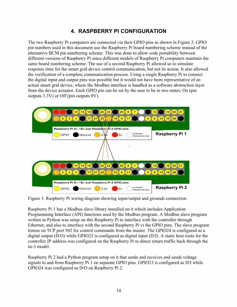
4. RASPBERRY PI CONFIGURATION The two Raspberry Pi computers are connected via their GPIO pins as shown in Figure 3. GPIO pin numbers used in this document use the Raspberry Pi board numbering scheme instead of the alternative BCM pin numbering scheme. This was done to allow code portability between different versions of Raspberry Pi since different models of Raspberry Pi computers maintain the same board numbering scheme. The use of a second Raspberry Pi allowed us to simulate response time for the smart grid device control communication, but not its action. It also allowed the verification of a complete communication process. Using a single Raspberry Pi to connect the digital input and output pins was possible but it would not have been representative of an actual smart grid device, where the Modbus interface is handled as a software abstraction layer from the device actuator. Each GPIO pin can be set by the user to be in two states; On (pin outputs 3.3V) or Off (pin outputs 0V).

Figure 3. Raspberry Pi wiring diagram showing input/output and grounds connection. Raspberry Pi 1 has a Modbus slave library installed on it which includes Application Programming Interface (API) functions used by the Modbus program. A Modbus slave program written in Python was setup on this Raspberry Pi to interface with the controller through Ethernet, and also to interface with the second Raspberry Pi vi the GPIO pins. The slave program listens on TCP port 502 for control commands from the master. The GPIO24 is configured as a digital output (D/O) while GPIO23 is configured as digital input (D/I). A static host route for the controller IP address was configured on the Raspberry Pi to direct return traffic back through the ns-3 model. Raspberry Pi 2 had a Python program setup on it that sends and receives and sends voltage signals to and from Raspberry Pi 1 on separate GPIO pins. GPIO23 is configured as D/I while GPIO24 was configured as D/O on Raspberry Pi 2.

15

5. INSTALLATION AND CONFIGURATION OF NS-3 The ns-3 network simulator (version 3.26) was downloaded and configured on the host server. When the simulator was bridged to the X-Net network, a packet length interpretation logic in the default ns-3 source code caused the ns-3 simulator to crash when packets were sent and received via the server’s bridged Ethernet adapter. This crash was caused by an internal software glitch in ns-3. The default ns-3 source code records the packet’s payload and checks to see if the payload is less than 1500 bytes in order to classify it as an IEEE 802.3 Ethernet packet. An IEEE 802.3 packet will also have an additional IEEE 802.2 Logical Link Control header. If it is an IEEE 802.3 packet, the logic then removes the header and trailer from the packet and checks to see if the resulting packet size is greater or equal to the payload size recorded. If this check fails, the simulator crashes. ns-3 does this check on packets received on Ethernet links to be able to distinguish IEEE 802.3 Ethernet protocol from other link layer protocols so as to apply the appropriate forwarding logic. The ns-3 source code was therefore modified to allow packets of any size to be exchanged between the external network and the simulated network. The modification does not affect packet processing in the ns-3 simulator but is a required workaround for the simulator to work with an actual physical Ethernet network. A topology generator written in Python (Appendix A) was installed on the host server. This program generates a random partial mesh topology which allows for network latency characterization under different topologies. A partially mesh network allows for some amount of redundant links to be in the topology but differs from a fully connected network topology. In a fully connected network topology, each node is redundantly connected to every other node in the topology which produces (n(n-1))/2 links where n is the number of nodes. Since RIP protocol uses hop count to choose best paths, partial mesh network topology was chosen to allow a sizable number of nodes to be traversed in the ns-3 network. This prevents the situation where a large portion of the network might become un-utilized. A partially connected network also presents a sparse edge network which is more representative of a real-world network. First, a 10-node circular connected graph is generated and 5 random nodes were selected and linked to form extra edges. For each of the two experiments conducted, the same number of nodes and links were used for the randomly generated topologies. This number is user-configurable and allows for flexibility in creating various topologies. To allow for the same topology and latencies to be generated in any future experiments, the program uses seed values that can be configured by a user. A seed value of 1 was used to generate the topologies used in the two experiments. The same seed values will produce the same topologies so that the same experiments can be repeated at later times. A network model was developed in ns-3 that utilizes randomly generated network topology. One node is always chosen from the ns-3 simulated network to be used for bridging to the external network; this effectively reduces the active nodes in the topology by one. The Modbus master client software is hosted on the server and utilizes the same Modbus library used on Raspberry Pi 1. This software serves as the Modbus master and sends a series of binary outputs to the Modbus slave. A single physical output bit is referred to as a coil in Modbus

16

protocol. A binary 1 signifies an “On” operation while a binary 0 signifies and “Off” operation on the Raspberry Pi computers. A static route for Raspberry Pi 1’s IP address is configured on the server to direct the control commands through the ns-3 model. This is required since there is no dynamic routing between the host server and the ns-3 network and ensures that traffic to and from the Raspberry Pi 1 is symmetrical. The symmetric nature of the routing is required to ensure that return traffic from the Modbus slave to the master goes through the ns-3 network so that latency can be more accurately characterized.

17

6. EXPERIMENTAL SETUP AND OBJECTIVES With the system setup in place, Monte Carlo simulations were conducted to estimate expected network latency on the wide-area grid control traffic. The experiment models direct load control [4] in demand response where Raspberry Pi 2 acts as a load that can be controlled by the electric utility. The utility sends control signals based on power demand and supply needs. The objective of the experiment is to probabilistically characterize network latency for wide-area grid control applications under various network assumptions. Based on link latencies in a specific topology, the experiments are expected to produce a range of round trip latencies from which a mean value can be estimated. As the testbed is flexible enough to be used to simulate various network topologies, experiments were conducted under several topologies as outlined in Table 1. The network topologies can be changed to model different scenarios. Table 1 Summary of experimental assumptions and reasoning Experiment #

Assumptions Reason for Assumption Resulting Round Trip Latency

1 Fixed network topology Mean latency on links set equal to N(µ = 6ms, s = 2ms). Bandwidth for all links set equal to 100Mbps

This mean latency was chosen to produce a round-trip latency similar to what is observed on wide-area networks [6]. Link bandwidth was chosen to be sufficiently large to avoid bandwidth limitations from interfering with our latency modeling methodology.

Average latency = N(µ = 204ms, s = 37ms) over 6 hops.

2 Randomly reconstruct a new topology with 10 nodes and 15 links for each Monte Carlo draw. In each draw, Modbus commands are sent over a specific network topology with link latencies described as follows: Mean latency on links set equal to N(µ = 8ms, s=3ms). Bandwidth for all links set equal to 100Mbps

Changing network paths based on instabilities in wide-area networks. Link bandwidth was chosen to be sufficiently large to avoid bandwidth limitations from interfering with our latency modeling methodology.

Average latency = N(µ = 321ms, s = 86ms) over variable number of hops. Min hop count is 5 and max hop count is 10.

In conducting the experiments, we assumed all links have large enough capacities as described in Table 1, with their respective latencies being a random variable sampled from a normal distribution, N(µ,s). This characterizes the link latency values of all links as a normal random variable chosen from the N(µ,s) distribution. However, actual wide-area networks are heterogeneous in nature and link latencies are not necessarily distributed normally around a

18

particular mean and standard deviation. But rather, it is more common to have each link latency normally distributed around a different mean and standard deviation based on the link type. If needed, this type of distribution can be modeled with minimal changes to the topology generation software. Another assumption used in this work is that no other traffic is traversing the network apart from the control traffic. However, most wide-area networks are used for transporting various types of data, which can impact latency based on queueing mechanisms used on routers. To make the emulation more realistic, additional traffic other than control traffic should be injected into the simulated network to make the modeling more realistic.

Figure 4. Fixed network topology used in ns-3 simulator for Experiment #1. The round-trip time for each control message was measured as shown in Figure 5. To measure the round-trip time, the Modbus master uses the server’s clock to first record the timestamp at which a control command was sent. When the Modbus master receives a response for the command, it again records the timestamp. The round-trip time is then measured by subtracting the command sent timestamp from the response received timestamp. For each control command sent, the round-trip latency was recorded and used to evaluate the latency distribution for the network topology used. The time series progression of a randomly selected single control message is shown in Figure 5.

19

From the time a control command is sent to the time a confirmation of command execution is received. It is observed that, regardless of the latency within the ns-3 topology, it typically takes less than 1ms for Raspberry Pi 1 to receive confirmation from Raspberry Pi 2 that a control command has been successfully processed. Such a processing time provides an opportunity to simulate fast IP-based network control. The system time for the Raspberry Pi 1 computers as well as the ns-3 server were synchronized to an external clock located on the same local area network using Network Time Protocol (NTP). Since NTP is precise to a few tens of milliseconds [8], the command processing times shown provide a rough estimate only.

Figure 5. Time series progression of a control message’s round-trip latency. 6.1 Experiment #1- Fixed Network Topology, Random Link Latencies This experiment assumed a fixed network topology to help characterize network latency under fixed topologies. Using the network topology generator, a 10-node partial mesh network was generated with 15 links. On each link in the topology, samples from a normal distribution (as described in Table 1) were used to specify the link latency. All links were configured with a very high bandwidth of 100 Mbps to avoid bandwidth limitations from affecting the modeling method, which is based on Probability Distribution Functions (PDFs). The topology in Figure 4 was used for Experiment #1. The arrows in Figure 4 show the path taken by the control messages

20

through the simulated ns-3 network. Return traffic from Raspberry Pi 2 flows symmetrically in the opposite direction of the arrows. In performing the Monte Carlo analysis on the topology shown in Figure 4, latencies for each link were generated according to a normal distribution, N(µ = 6ms, s = 2ms), as outlined in Experiment #1 of Table 1. This creates a probability distribution for the latencies on each link which, when sampled, produces different possible latency outcomes. The experiment was repeated using 100 sample sets of latencies and it took about 7hours to complete. For each sample set, the controller sent 200 control messages to the Raspberry Pi 2 through the simulated network. This makes a total of 20,000 (100 x 200) control messages for the entire experiment. Figure 6 shows the latency Cumulative Distribution Function (CDF) and PDF for all the latencies measured in Experiment #1. From the latency PDFs shown in Figure 6, the mean round-trip communication latency of 204ms with a standard deviation of 37ms. This gives a good estimation of latency range within which the smart grid device can be controlled given the network topology used. This result can be used as input in building a stable control system. Furthermore, when the monitoring of latency is done in real-time in an operational control system, the results can be used to detect abnormal network performance, and subsequent control system performance. Such abnormal performance can result from cyber security attacks in the network, link congestion issues or sub-optimal performance of the routers in the network.

Gaussian PDF Fit and Normalized Histogram of Experiment 1 Network LatenciesN( =0.20398 sec, =0.036985 sec), n=20,000, 250 bins

0.05 0.1 0.15 0.2 0.25 0.3 0.35 0.4 0.45Latency [sec]

0

5

10

15

20

25

Prob

abilit

y

Gaussian CDF Fit and Normalized Data of Experiment 1 Network LatenciesN( =0.20398 sec, =0.036985 sec), n=20,000

0.05 0.1 0.15 0.2 0.25 0.3 0.35 0.4 0.45Latency [sec]

0

0.2

0.4

0.6

0.8

1

Cum

ulat

ive D

ensit

y

Figure 6. CDF and PDF plots of measured round-trip latencies for Experiment #1.

21

6.2 Experiment #2 - Random Network Topology with Random Link Delays This experiment assumed network topology changes for each sampled link latency set to help characterize network latency under unstable topologies. A randomly generated 10-node partial mesh network with 15 links was used for each run. On each link in the topology, latency values were generated according to a normal distribution with chosen mean and standard deviation as described in Table 1. All links were configured with a bandwidth of 100Mbps to avoid bandwidth restrictions from affecting our modeling method which is based on latency. By performing Monte Carlo experiments, different latencies on the links were generated according to a normal distribution, N(µ = 8ms, s = 3ms), as outlined in Experiment #2 of Table 1. This creates a probability distribution for the latencies on each link which produces different possible latency outcomes. The experiment was repeated for 85 times with the controller sending 200 control messages to the Raspberry Pi 2 for each run through the simulated network. This represents a total of 17,000 control messages for the entire experiment. It took approximately 7hours for this experiment to complete. The round-trip latency for each control message was measured. Figure 7 shows the latency CDF and PDF for all the latencies measured in Experiment #2.

Gaussian PDF Fit and Normalized Histogram of Experiment 2 Network LatenciesN( =0.32136sec, =0.086183 sec), n=17,000, 250 bins

0 0.1 0.2 0.3 0.4 0.5 0.6 0.7 0.8 0.9 1Latency [sec]

0

2

4

6

8

Prob

abilit

y

Gaussian CDF Fit and Normalized Data of Experiment 2 Network LatenciesN( =0.32136sec, =0.086183 sec), n=17,000

0 0.1 0.2 0.3 0.4 0.5 0.6 0.7 0.8 0.9 1Latency [sec]

0

0.5

1

1.5

Cum

ulat

ive

Den

sity

Figure 7. CDF and PDF plots of measured round-trip latencies for Experiment #2.

22

From the latency PDFs shown in Figure 7, it can be observed that by varying the topologies for each sample set of latency distribution, the mean round-trip communication latency is 321 ms with a standard deviation of 86 ms. A comparison of the latency distributions for the two experiments, depicted in Figure 8, shows a much larger standard deviation for Experiment #2, where random topologies were reconstructed for each sampled link latency set.

Figure 8. Latency distribution comparison between Experiments 1 and 2.

23

7. SUMMARY AND FUTURE WORK

This project developed capability to support research in network latency characterization in wide–area network [6] grid control applications. We built a testbed that can be used to model and probabilistically characterize network latency under various conditions. Latency information is needed to support the design of IP based feedback control systems over wide-area networks. We performed two main tasks in this project. The first task was to develop an experimental platform (testbed). The second task was to use the testbed to conduct stochastic characterization of network latency through experimentation. The experiments were conducted under various conditions based on assumptions described in Table 1. By undertaking this project, we aimed to develop the capability to enable the effective design of IP-based feedback control systems for the smart grid. Without the ability to properly design a control system quantifying feedback delays, it will not be possible to predict system stability under the operation of that control system. The use of a simulator provides a cost-effective way of conducting experiments that model simple as well as complex network topologies. As shown in the results of Experiment #2, randomization of network topology links result in a much larger standard deviation of network latency. This is expected since modifying topologies will result in routing changes where packets will have to take other paths which might inadvertently have shorter or longer round-trip latencies. In future work, the effect of cyber-attack scenarios such as Denial of Service (DoS) could be incorporated in the simulation, while using more comprehensive network architectures. Also, simulations could be conducted using Named Data Networking (NDN) [5] architecture based on Information Centric Networking (ICN). The experimental results could be compared with host-centric IP architecture. Additionally, link failures and subsequent network convergence scenarios could be modeled to evaluate their effect on grid traffic. Another future work could entail setting up time synchronization between all the devices in the testbed to millisecond accuracy so that control command processing and action times can be determined with more granularity and accuracy. Due the use of hardware (Raspberry Pi), the testbed is limited to the design of a control system where the controller is able to control only a single smart grid device. As it is quite inexpensive to expand the testbed with additional Raspberry Pi computers, it would not take a large investment to experiment with more smart grid devices so as to be able to characterize latency under such a condition.

24

8. CONCLUSION

Grid modernization presents new research challenges to determine how various sub-systems of the electric grid can interact to provide effective and enhanced services. The manner in which grid sub-systems communicate over the network affects the efficacy of controls systems for the electric grid. Combining software-based network simulation with hardware devices creates unique research platform for smart grid communications research, including the stochastic modeling of network latency. Researchers are able to model network communication systems and gain valuable information to aid them in the design of control systems; including the ability to stochastically quantify network latency. Such information is fundamental toward quantitatively bounding the stability of a closed loop feedback control system connected to an IP-based network.

25

REFERENCES

[1] Discrete-event network simulator for Internet systems. https://www.nsnam.org [2] Python implementation of the Modbus protocol. http://umodbus.readthedocs.io/en/latest/ [3] Raspberry Pi: Single-board computer. http://umodbus.readthedocs.io/en/latest/ [4] Demand response. https://energy.gov/oe/activities/technology-development/grid-modernization-and-smart-grid/demand-response [5] Spyridon Mastorakis, Alexander Afanasyev, Ilya Moiseenko, and Lixia Zhang. 2016. ndnSIM 2: An updated NDN simulator for ns-3. Technical Report NDN-0028, Revision 2. NDN. [6] Carter, Robert L., and Mark E. Crovella. "Server selection using dynamic path characterization in wide-area networks." In INFOCOM'97. Sixteenth Annual Joint Conference of the IEEE Computer and Communications Societies. Driving the Information Revolution., Proceedings IEEE, vol. 3, pp. 1014-1021. IEEE, 1997. [7] Network Time Protocol Version 4. https://www.ietf.org/rfc/rfc5905.txt [8] Modbus protocol. http://www.modbus.org/specs.php [9] J. F. Kurose and K. W. Ross, Computer Networking: A Top-Down Approach. Addison Wesley, 7th edition.

26

27

APPENDIX

A. SERVER SETUP

i) ns-3 Installation and Compilation

1. Open a new terminal window on the Ubuntu server 2. Create a new directory to host ns-3: mkdir ns3 (you can use any name for directory) 3. Switch to the new directory created: cd ns3 4. Download ns-3 source code (version 2.6): wget https://www.nsnam.org/release/ns-allinone-3.26.tar.bz2 5. Extract the contents of the downloaded file: tar -jxvf ns-allinone-3.26.tar.bz2 6. Switch directory: cd ns-allinone-3.26/ns-3.26 7. Configure the ns-3 source code: ./waf configure --enable-examples --enable-tests --enable-sudo

This process should show 'configure' finished successfully when done. Ignore other errors. If you don't see this message, it means configuration failed. Analyze the logs to see which packages may have filed during compilation and install them.

8. Compile ns-3: ./waf This will take some time to complete. Test if installation is successful by running ./waf --run hello-simulator. You should see the output "Hello Simulator".

ii) Modify ns-3 for External Network Bridging

1. Open ns-3 source code the file: nano src/csma/model/csma-net-device.cc 2. On line 756 or the line starting with "if (header.GetLengthType () <= 1500)", comment out the whole True block logic of the "if statement" 3. Copy the line "protocol = header.GetLengthType ();" from the Else block and put it in the True block.

Save file using Ctrl+O and press enter Exit file editing using Ctrl+S Use this same save and exit instruction for all files modified using "nano" editor

iii) Install Bridge Utilities for External Network Connectivity

1. Install Linux bridge utilities: sudo apt-get install bridge-utils 2. Install tunctl: sudo apt-get install uml-utilities 3. Backup the network original configuration: sudo cp /etc/network/interfaces /etc/network/interfaces.original 4. Create a new file named /etc/network/interfaces.ns3.bridge as below (eno1 is the network adaptor name, change to the name of the one you want to use on your server): sudo nano /etc/network/interfaces.ns3.bridge 5. Enter the following into the file, this create a Linux bridge used to connect the ns-3 network to the external network: auto eno1

28

iface eno1 inet manual auto br-trigger iface br-trigger inet manual bridge_ports eno1

iv) Linux Bridge Setup Scripts

Files names should be spelled correctly otherwise scripts will not work, if you change any file name ensure the corresponding references to the names changed also. 1. Change directory: cd ns3/ns-allinone-3.26/ns-3.26/src/tap-bridge/examples 2. Using nano or other text editor, create file named "demand-response-setup.sh" with below: #!/bin/sh brctl addbr br-outif tunctl -t tap-outif tunctl -t tap-inif ifconfig tap-outif 0.0.0.0 promisc up ifconfig tap-inif 0.0.0.0 promisc up brctl addif br-outif tap-outif brctl addif br-outif tap-inif ifconfig br-outif up 3. Create file named "demand-response-teardown.sh" with below: #!/bin/sh ifconfig br-outif down brctl delif br-outif tap-outif brctl delif br-outif tap-inif brctl delbr br-outif ifconfig tap-outif down ifconfig tap-inif down tunctl -d tap-outif tunctl -d tap-inif 4. For both files, enable executable permission on them using: sudo chmod 777 <filename>

v) Script to Automatically Bridge ns-3 to External Network 1. Create a directory called “Project-218” in the home directory of the server 2. Switch to this directory. This script consigures static IP of 10.1.8.41 on server. The ns-3 node bridged to this subnet has IP 10.1.8.42 3. Create file "bridge-to-ns3.sh" with below contents and give it executable permission

29

../ns3/ns-allinone-3.26/ns-3.26/src/tap-bridge/examples/demand-response-setup.sh cp /etc/network/interfaces.ns3.bridge /etc/network/interfaces sudo ifconfig eno1 0.0.0.0 sudo ifconfig br-outif 10.1.8.41/24 route add -net 0.0.0.0/0 gw 10.1.8.254 route add -host 10.1.8.45 gw 10.1.8.42

vi) Script to Automatically Remove ns-3 Bridge from External Network 1. Create file "unbridge-from-ns3.sh" with below contents and give it executable permission ../ns3/ns-allinone-3.26/ns-3.26/src/tap-bridge/examples/demand-response-teardown.sh cp /etc/network/interfaces.original /etc/network/interfaces sudo ifconfig eno1 down sudo service network-manager stop sudo ifconfig eno1 up sudo service network-manager start

vii) Install Modbus Library sudo pip install uModbus

viii) Create Modbus Master Application 1. Create file named "master-modus.py" with below content #!/usr/bin/env python import socket import datetime import time from umodbus import conf from umodbus.client import tcp # Enable values to be signed (default is False). conf.SIGNED_VALUES = True sock = socket.socket(socket.AF_INET, socket.SOCK_STREAM) sock.connect(('10.1.8.45', 502)) # Build on/off load commands control_cmd = [] switchon = True for i in range(0,200): if switchon:

30

control_cmd.append(1) switchon = False else: control_cmd.append(0) switchon = True outfile = open('/home/conet1502/Project-218/results/timestamps_modbus_master_' + str(time.time()) + '.csv','w') outfile.write('timestamp,round_trip_time,control_command,command_status,type\n') latsum = 0.0 latcount = 0 for j in range(0,len(control_cmd)): # Returns a message or Application Data Unit (ADU) specific for doing # Modbus TCP/IP. coil_write_msg = tcp.write_multiple_coils(slave_id=1, starting_address=0, values=control_cmd[j:j+1]) start_time = time.time() print datetime.datetime.now().strftime('%Y-%m-%d %H.%M.%S.%f'), '', control_cmd[j], '','write' outfile.write(str(datetime.datetime.now().strftime('%Y-%m-%d %H.%M.%S.%f')) + ',' + '' + ',' + str(control_cmd[j]) + ',' + '' + ',write\n') # Response depends on Modbus function code. This particular returns the # amount of coils written, in this case it is. coil_write_rsp = tcp.send_message(coil_write_msg, sock) #Read received voltage on pin 16 coil_read_msg = tcp.read_coils(slave_id=1, starting_address=0, quantity=1) coil_read_rsp = tcp.send_message(coil_read_msg, sock) rtt = time.time() - start_time print datetime.datetime.now().strftime('%Y-%m-%d %H.%M.%S.%f'), rtt, '', coil_read_rsp[0],'read' outfile.write(str(datetime.datetime.now().strftime('%Y-%m-%d %H.%M.%S.%f')) + ',' + str(rtt) + ',' + '' + ',' + str(coil_read_rsp[0]) + ',read\n') latsum += rtt latcount += 1 expfile = open('/home/conet1502/Project-218/results/temp_exp.csv','a')

31

expfile.write(str(latsum/latcount) + '\n') expfile.close() outfile.close() sock.close()

ix) Create Topology Generator Script 1. Create file named "topogen.py" with below content import random import sys import numpy as np random.seed(1) numofnodes = 10 link_bw = 100 edgecounter = 1 edgeproperty = '' tap1_subnet = '10.1.8.40' tap2_subnet = '10.1.8.44' edge_subnet = '192.168.1.0' subnet_mask = '255.255.255.252' ip_octets = [] next_subnet = '' ns3extnode1 = 0 ns3extnode2 = 0 skipedge = False minlatency = 1 maxlatency = 10 maxextraedges = 5 outfile = open('demand-response-topo.txt','w') outfile.write(str(numofnodes) + ' x ' + ' x ' + ' x ' + ' x ' + ' x \n') print str(numofnodes) + ' x ' + ' x ' + ' x ' + ' x ' + ' x' graphedges = [] graphedges.append((0,1)) graphedges.append((0,2)) for i in range(2,numofnodes): if i == (numofnodes - 1): graphedges.append((1,numofnodes-1)) else: graphedges.append((i,i+1))

32

#Randomly attach up to 'maxextraedges' variable set above extraedgecounter = 0 extraedgecount = numofnodes - 4 for k in range(0,(((extraedgecount*(extraedgecount-1))/2) - (extraedgecount-1))): if extraedgecounter < maxextraedges: randnode1 = random.randint(3,numofnodes-2) randnode2 = random.randint(3,numofnodes-2) if randnode1 == randnode2: pass elif randnode1 + 1 == randnode2: pass elif randnode1 - 1 == randnode2: pass else: if randnode1 < randnode2: if not ((randnode1,randnode2) in graphedges): graphedges.append((randnode1,randnode2)) extraedgecounter += 1 else: if not ((randnode2,randnode1) in graphedges): graphedges.append((randnode2,randnode1)) extraedgecounter += 1 else: #Do not connect any extra edges break for edge in graphedges: if edgecounter == 1: edgeproperty = str(edge[0]) + ' ' + str(edge[1]) + ' ' + str(0) + ' ' + str(link_bw) + ' ' + tap1_subnet + ' ' + subnet_mask ns3extnode1 = edge[1] edgecounter += 1 elif edgecounter == 2: edgeproperty = str(edge[0]) + ' ' + str(edge[1]) + ' ' + str(0) + ' ' + str(link_bw) + ' ' + tap2_subnet + ' ' + subnet_mask ns3extnode2 = edge[1] edgecounter += 1 else: if (int(edge[0]) == int(ns3extnode1) and int(edge[1]) == int(ns3extnode2)) or (int(edge[0]) == int(ns3extnode2) and int(edge[1]) == int(ns3extnode1)): #Skip the interconnection between the ns-3 nodes bridged to the LAN (allows remaining topology to be traversed) skipedge = True

33

elif int(edge[0]) == 0: #Skip all other connectons to node 0 skipedge = True else: ip_octets = edge_subnet.split('.') if int(ip_octets[3]) <= 252: #Fourth octet has usable subnet next_subnet = ip_octets[0] + '.' + ip_octets[1]+ '.' + ip_octets[2] + '.' + str(ip_octets[3]) edgeproperty = str(edge[0]) + ' ' + str(edge[1]) + ' ' + str(0) + ' ' + str(link_bw) + ' ' + next_subnet + ' ' + subnet_mask edge_subnet = ip_octets[0] + '.' + ip_octets[1]+ '.' + ip_octets[2] + '.' + str(int(ip_octets[3]) + 4) else: #Increase third octet IP by 1 if int(ip_octets[2]) < 255: next_subnet = ip_octets[0] + '.' + ip_octets[1]+ '.' + str(int(ip_octets[2]) + 1) + '.' + '0' edgeproperty = str(edge[0]) + ' ' + str(edge[1]) + ' ' + str(0) + ' ' + str(link_bw) + ' ' + next_subnet + ' ' + subnet_mask edge_subnet = ip_octets[0] + '.' + ip_octets[1]+ '.' + str(int(ip_octets[2]) + 1) + '.' + '4' else: #Stop subnet allocation!!! You've run out of private class C address print 'You have run out of private class C address: 192.168.x.x Too many edges in graph' sys.exit() if skipedge == True: skipedge = False else: print edgeproperty outfile.write(edgeproperty + '\n') outfile.close() #Generate latency file according to random normal distribution latdist = [] numofexp = 100 latfile = open('latencies.txt','w') #Generate random uniform edge latencies for edge in range(0, (numofnodes+maxextraedges)): mean = 6 stddev = 2 #print mean, stddev latdist.append(np.random.normal(mean,stddev,numofexp)) #Generate edges for number of experiments to run for i in range(0,numofexp):

34

for j in range(0,len(latdist)): latfile.write(str(int(latdist[j][i]))) if j < len(latdist) - 1: latfile.write(',') latfile.write('\n') latfile.close()

x) Create ns-3 Scenario File 1. Switch to ns-3 directory: cd ns3/ns-allinone-3.26/ns-3.26/scratch 2. Create the scenario file named "demand-response-sim.cc" with below contents // This is network model used as a backbone network for sending control commands. // It is bridged to the physical network as the packets are source from external computer and destined to an external device // Routing is first done through this network model and may be handed off to WAN to destinations outside the LAN #include <iostream> #include <fstream> #include <sstream> #include "ns3/core-module.h" #include "ns3/network-module.h" #include "ns3/csma-module.h" #include "ns3/tap-bridge-module.h" #include "ns3/internet-module.h" #include "ns3/netanim-module.h" #include "ns3/point-to-point-module.h" #include "ns3/point-to-point-net-device.h" #include "ns3/olsr-helper.h" #include "ns3/rip-helper.h" using namespace ns3; NS_LOG_COMPONENT_DEFINE ("DemandResponseSimulation"); //Declare global variables NodeContainer nodes; CsmaHelper csma; PointToPointHelper p2p; Ipv4StaticRoutingHelper ipv4RoutingHelper; int nodecount = 0, tapnode1 = 0, tapnode2 = 0; std::string topologyfile = "/home/conet1502/Project-218/demand-response-topo.txt"; int

35

main (int argc, char *argv[]) { std::vector<std::string> edgelatencies; std::string strLatency = ""; // Create command line argument (these are the latencies on the links, comma separated) CommandLine cmd; cmd.AddValue("strLatency", "Latencies of the various edges", strLatency); cmd.Parse (argc, argv); //Split the latencies by the comma separator std::istringstream ss(strLatency); std::string token; while(std::getline(ss, token, ',')) { edgelatencies.push_back(token); } // // We are interacting with the outside, real, world. This means we have to // interact in real-time and therefore means we have to use the real-time // simulator and take the time to calculate checksums. // GlobalValue::Bind ("SimulatorImplementationType", StringValue ("ns3::RealtimeSimulatorImpl")); GlobalValue::Bind ("ChecksumEnabled", BooleanValue (true)); // Get node count as well as tap-bridge nodes std::string srcnode, dstnode, latency, bw, subnet, netmask; int edgecounter = 1, edgenum = 0; std::ifstream inpfile1 (topologyfile, std::ios::in); if (inpfile1.is_open ()) { while (inpfile1 >> srcnode >> dstnode >> latency >> bw >> subnet >> netmask ) { if (edgecounter == 1) { nodecount = stoi(srcnode); edgecounter += 1; } else if (edgecounter == 2) { tapnode1 = stoi(dstnode); edgecounter += 1; } else if (edgecounter == 3) {

36

tapnode2 = stoi(dstnode); //Reset edge counter, used same variable in next file iteration edgecounter = 1; break; } } } else { std::cout << "Error::Cannot open topology file!!!" << std::endl; return 1; } inpfile1.close(); //NodeContainer nodes; nodes.Create (nodecount); // Enable RIP NS_LOG_INFO ("Enabling RIP Routing."); ns3::RipHelper ripRouting; //Exclude bridged interfaces from exchanging RIP updates ripRouting.ExcludeInterface (nodes.Get(tapnode1), 1); ripRouting.ExcludeInterface (nodes.Get(tapnode2), 1); Ipv4ListRoutingHelper listRH; listRH.Add (ipv4RoutingHelper, 0); listRH.Add (ripRouting, 10); InternetStackHelper internet; internet.SetRoutingHelper (listRH); internet.Install (nodes); Ipv4AddressHelper addresses; NetDeviceContainer devices1; NetDeviceContainer devices2; std::ifstream inpfile2 (topologyfile, std::ios::in); if (inpfile2.is_open ()) { while (inpfile2 >> srcnode >> dstnode >> latency >> bw >> subnet >> netmask ) { if (edgecounter == 1) { //Ignore first line, countains number of nodes in graph edgecounter += 1; }

37

else if (edgecounter == 2) { NodeContainer tappair1; tappair1.Add (nodes.Get(0)); tappair1.Add (nodes.Get(tapnode1)); csma.SetChannelAttribute ("DataRate", DataRateValue (stoi(bw)*1000000)); csma.SetChannelAttribute ("Delay", TimeValue (MilliSeconds (stoi(edgelatencies[edgenum])))); devices1 = csma.Install (tappair1); addresses.SetBase (Ipv4Address (subnet.c_str()), Ipv4Mask(netmask.c_str())); Ipv4InterfaceContainer interfaces1 = addresses.Assign (devices1); edgecounter += 1; edgenum += 1; } else if (edgecounter == 3) { NodeContainer tappair2; tappair2.Add (nodes.Get(0)); tappair2.Add (nodes.Get(tapnode2)); csma.SetChannelAttribute ("DataRate", DataRateValue (stoi(bw)*1000000)); csma.SetChannelAttribute ("Delay", TimeValue (MilliSeconds (stoi(edgelatencies[edgenum])))); devices2 = csma.Install (tappair2); addresses.SetBase (Ipv4Address (subnet.c_str()), Ipv4Mask(netmask.c_str())); Ipv4InterfaceContainer interfaces2 = addresses.Assign (devices2); edgecounter += 1; edgenum += 1; } else { //Connect ns-3 edges only from now NodeContainer nodepair; nodepair.Add (nodes.Get(stoi(srcnode))); nodepair.Add (nodes.Get(stoi(dstnode))); p2p.SetDeviceAttribute ("DataRate", StringValue (bw + "Mbps")); p2p.SetChannelAttribute ("Delay", StringValue(edgelatencies[edgenum] + "ms")); NetDeviceContainer devices = p2p.Install (nodepair); addresses.SetBase (Ipv4Address (subnet.c_str()), Ipv4Mask(netmask.c_str())); Ipv4InterfaceContainer interfaces = addresses.Assign (devices); edgenum += 1; } }

38

} inpfile2.close(); //Configure default route on exit node ripRouting.SetDefaultRouter (nodes.Get(tapnode2), Ipv4Address ("10.1.8.45"), 1); //Bridge node 0 to the physical NIC of server TapBridgeHelper tapBridge; tapBridge.SetAttribute ("Mode", StringValue ("UseBridge")); tapBridge.SetAttribute ("DeviceName", StringValue ("tap-outif")); tapBridge.Install (nodes.Get (0), devices1.Get (0)); tapBridge.SetAttribute ("DeviceName", StringValue ("tap-inif")); tapBridge.Install (nodes.Get (0), devices2.Get (0)); //Print out the routing table on all nodes Ipv4GlobalRoutingHelper globalRouting; Ptr<OutputStreamWrapper> routingStream = Create<OutputStreamWrapper> ("routing-tables.routes", std::ios::out); globalRouting.PrintRoutingTableAllAt (Seconds(180.0), routingStream ); // // Run the simulation for one hour to give the user time to play around // Simulator::Stop (Seconds (120.)); Simulator::Run (); Simulator::Destroy (); }

xi) Create Experiment Automation Script 1. Create a file name “automate.py” with contents import sys import os import multiprocessing import time latfile = open("/home/conet1502/Project-218/latencies.txt","r") def start_ns3(line): print 'Starting ns3 with edge latencies', line os.system('./waf --run "demand-response-sim --strLatency=' + line + '"') def start_modbus(counter): print 'Starting modbus master...'

39

os.system('python /home/conet1502/Project-218/master-modbus.py') print '\nCompleted experiment', counter, 'Waiting 50sec to start next one...\n' #Timer waits for ns3 to automatically terminate time.sleep(120) def clean_up(): p1.terminate() p1.join() if __name__=='__main__': global p1 try: expcount = 1 for line in iter(latfile): p1 = multiprocessing.Process(target=start_ns3, args =(line.strip(),)) p1.start() #Timer waits for ns3 to completely start before sending control signals time.sleep(20) start_modbus(expcount) clean_up() expcount += 1 finally: os.system('mv /home/conet1502/Project-218/results/temp_exp.csv /home/conet1502/Project-218/results/average_latencies_' + str(time.time()) + '.csv') print 'Simulation completed successfully'

B. RASPBERRY PI 1 SETUP

i) Installation of Modbus Library 1. sudo pip install --upgade pip (This is required else the uModbus will not install via pip) 2. sudo pip install uModbus

ii) Create the Modbus Slave Application 1. Create a file name “slave-modbus.py” with contents #!/usr/bin/env python import logging from SocketServer import TCPServer from collections import defaultdict from umodbus import conf

40

from umodbus.server.tcp import RequestHandler, get_server from umodbus.utils import log_to_stream import RPi.GPIO as GPIO import datetime import time import multiprocessing import sys import os #Declare Raspberry Pi GPIO board numbering GPIO.setmode(GPIO.BOARD) #Set intial GPIO pin modes GPIO.setup(18, GPIO.OUT, initial=GPIO.LOW) GPIO.setup(16, GPIO.IN, pull_up_down = GPIO.PUD_UP) # Add stream handler to logger 'uModbus'. log_to_stream(level=logging.DEBUG) # A very simple data store which maps addresses against their values. data_store = defaultdict(int) # Enable values to be signed (default is False). conf.SIGNED_VALUES = True filetimstamp = time.time() outfile = open('results/timestamps_modbus_slave_' + str(filetimstamp) + '.csv','w') outfile.write('timestamp,control_command,type\n') TCPServer.allow_reuse_address = True app = get_server(TCPServer, ('10.1.8.45', 502), RequestHandler) print "Slave is ready and waiting for commands..." @app.route(slave_ids=[1, 2], function_codes=[1, 2], addresses=list(range(0, 10))) def read_data_store(slave_id, function_code, address): """" Return value of address. """ return GPIO.input(16) #data_store[address] @app.route(slave_ids=[1, 2], function_codes=[5, 15], addresses=list(range(0, 10))) def write_data_store(slave_id, function_code, address, value): """" Set value for address. """ print 'Command received from master, value = ', value, datetime.datetime.now() outfile.write(str(datetime.datetime.now().strftime('%Y-%m-%d %H.%M.%S.%f')) + ',' + str(value) + ',command_received_from_master\n')

41

# Send output voltage via Raspberry1 GPIO if value == 1: print 'Voltage sent to load, set pin 18 output to', value, datetime.datetime.now() outfile.write(str(datetime.datetime.now().strftime('%Y-%m-%d %H.%M.%S.%f')) + ',' + str(value) + ',command_sent_to_rp2\n') GPIO.output(18, GPIO.HIGH) else: print 'Voltage sent to load, set pin 18 output to', value, datetime.datetime.now() outfile.write(str(datetime.datetime.now().strftime('%Y-%m-%d %H.%M.%S.%f')) + ',' + str(value) + ',command_sent_to_rp2\n') GPIO.output(18, GPIO.LOW) def check_input_pin_status(pinvalue): try: tmpfile = open('results/z_temp_file.csv','w') while True: if GPIO.input(16) != pinvalue: print 'Successfully set voltage to', GPIO.input(16), datetime.datetime.now() tmpfile.write(str(datetime.datetime.now().strftime('%Y-%m-%d %H.%M.%S.%f')) + ',' + str(GPIO.input(16)) + ',response_received_from_rp2\n') pinvalue = GPIO.input(16) except: tmpfile.close() finally: tmpfile.close() if __name__ == '__main__': global p1 try: #Start separate process to check when input pin status changes p1 = multiprocessing.Process(target=check_input_pin_status, args=(GPIO.input(16),)) p1.start() #Main program process receives master commands app.serve_forever() except KeyboardInterrupt: pass except: pass finally: p1.terminate() p1.join() app.shutdown() app.server_close()

42

outfile.close() os.system('more results/z_temp_file.csv >> ' + ' results/timestamps_modbus_slave_' + str(filetimstamp) + '.csv') os.system('rm results/z_temp_file.csv') GPIO.output(18, GPIO.LOW) GPIO.setup(16, GPIO.IN, pull_up_down = GPIO.PUD_UP) GPIO.cleanup() print 'Program exited by user!!! - Raspberry Pi1'

iii) IP Configuration 1. Disable dhcpcd service: systemctl disable dhcpcd.service 2. Assign static IP to the network interface. Edit the file “/etc/network/interfaces” with below content. The ns-3 node bridged to this subnet has IP 10.1.8.46 auto eth0 iface eth0 inet static address 10.1.8.45 netmask 255.255.255.0 gateway 10.1.8.254 dns-nameservers 10.255.255.2 3. Reboot the Raspberry Pi for configuration changes to take effect. NB: re-add static route each time you reboot, as this configuration is lost after every reboot 4. Configure static route through ns-3 topology: sudo route add -host 10.1.8.41 gw 10.1.8.46

C. RASPBERRY PI 2 SETUP

i) Create Application for the Controlled Device 1. Create a file name “voltage-signals.py” with below contents. This sends and receives voltage pulses from Raspberry Pi 1 over the GPIO pins. import RPi.GPIO as GPIO import time import datetime def voltage_send_receive(): GPIO.setmode(GPIO.BOARD) GPIO.setup(18, GPIO.OUT, initial=GPIO.LOW) GPIO.setup(16, GPIO.IN, pull_up_down = GPIO.PUD_UP)

43

inputpinvalue = GPIO.input(16) while True: if GPIO.input(16) != inputpinvalue: print 'Pin 16 received ', GPIO.input(16), datetime.datetime.now() GPIO.output(18, GPIO.input(16)) print 'Pin 18 set to', GPIO.input(18), datetime.datetime.now() inputpinvalue = GPIO.input(16) if __name__ == '__main__': try: print 'Waiting to receive signals' voltage_send_receive() except KeyboardInterrupt: pass except: pass finally: GPIO.output(18, GPIO.LOW) GPIO.setup(16, GPIO.IN, pull_up_down = GPIO.PUD_UP) GPIO.cleanup() print 'Program exited by user!!! - Raspberry Pi2'

D. EXPERIMENTS, USER CONFIGURATIONS AND MISCELLANEOUS

i) How to Run Experiments 1. Generate the network topology on server by changing directory to “Project-218” and running the script: python topogen.py 2. Logon to Raspberry Pi 2 and start the application that sends and receive the voltage pulses: python voltage-signals.py 3. Logon to Raspberry Pi 1 and start the Modbus slave application sudo python slave-modbus.py 4. On the server, switch to below directory and execute the automation script to run repeated experiments based on the number specified by the user in the topology generation script cd /ns3/ns-allinone-3.26/ns-3.26 python automate.py 5. The average latencies for each run of the experiment are saved on the server with a file name starting with “average_latencies_” and a system generated timestamp. This file is located in the directory “Project-218/results”

44

ii) User Configurable Parameters

1. Number of nodes in topology. In the file “topogen.py” change the value of the variable named "numofnodes" 2. Number times to repeat experiment with different latencies. In the file “topogen.py” change the value of the variable named "numofexp" 3. Mean value for the latency distribution on links. In file “topogen.py” change the value of the variable named "mean" 4. Standard deviation for latency distribution on links. In file “topogen.py” change the variable name "stddev" 5. How long to run each run of ns-3 topology with specific link latencies.

In the ns-3 scenario file “scratch/demand-response-sim.cc” change the decimal value in the line “Simulator::Stop (Seconds (120.));”

iii) MATLAB Code For PDF and CDF

load latencydata.mat ndist_lf=fitdist(latency_fixed,'Normal') x_values = 0.05:.001:.5; y = pdf(ndist_lf,x_values); subplot(2,1,1); plot(x_values,y,'LineWidth',2); hold; histogram(latency_fixed,50,'Normalization','pdf'); title(['Gaussian PDF Fit and Normalized Histogram of Network Latencies' char(10) 'N(\mu=' num2str(ndist_lf.mu) ', \sigma=' num2str(ndist_lf.sigma) ')']) xlabel('Latency [sec]');ylabel('Probability'); grid on;hold off subplot(2,1,2);histogram(latency_fixed,50,'Normalization','cdf'); hold;grid on; subplot(2,1,2);%cdfplot(latency_fixed); y=cdf('Normal',x_values,ndist_lf.mu,ndist_lf.sigma); subplot(2,1,2);plot(x_values,y,'LineWidth',2) title(['Gaussian CDF Fit and Normalized Data of Network Latencies' char(10) 'N(\mu=' num2str(ndist_lf.mu) ', \sigma=' num2str(ndist_lf.sigma) ')']) xlabel('Latency [sec]');ylabel('Cumulative Density'); hold off

45

46

DISTRIBUTION 1 MS1033 Ross Guttromson Org. Number 08812 (electronic copy) 1 MS1033 Jay Johnson Org. Number 08812 (electronic copy) 1 MS1033 Abe Ellis Org. Number 08812 (electronic copy) 1 MS10xx Ray Byrne Org. Number 08813 (electronic copy) 1 MS0899 Technical Library 9536 (electronic copy)

47