stochastic channel model for dense urban line-of … · stochastic channel model for dense urban...

1

EUROPEAN COOPERATION

IN THE FIELD OF SCIENTIFIC

AND TECHNICAL RESEARCH

—————————————————

EURO-COST

—————————————————

COST 2100 TD(07)041 Lisbon, Portugal 2007/Febr/26-28

SOURCE: Department of International Development Engineering, Tokyo Institute of Technology, Japan

Stochastic Channel Model for Dense Urban Line-of-Sight Street Microcell

Mir Ghoraishi 214, S6 Bldg, 2-12-1-S6-4 Ookayama, meguro-ku Tokyo, 152-8550 JAPAN Phone: + 81-3 5734 3288 Fax: + 81-3 5734 3288 Email: [email protected]

Stochastic Channel Model for Dense UrbanLine-of-Sight Street Microcell

Mir Ghoraishi Jun-ichi Takada

Department of International Development EngineeringTokyo Institute of Technology

Tokyo, 152-8550, [email protected], [email protected]

Tetsuro Imai

R&D CenterNTT DoCoMo Inc.

Kanagawa, 239-8536, [email protected]

ABSTRACT

A stochastic channel model for line-of-sight (LoS) street microcell scenarios in dense urbanareas is proposed. The scattering power distribution (SPD)in the channel seen from the mobileterminal (MT) based on the physical phenomenon is obtained.The coefficients of the distributionare derived by approximation to the measurements performedin urban street microcell scenarios.The azimuth-power spectrum (APS) and the power-delay profile (PDP) predicted by the proposedmodel is compared to those for conventional model as well as to the experimental results. It isshown that the proposed model in contrast to the conventional models produces results that closelyagree with the experiments.

I. I NTRODUCTION

Characterization and modeling of the radio propagation channel are essential for mobile andwireless systems design. A detailed knowledge about mobilecommunication propagation channelleads to a more successful design of the communication system. Especially to design and evaluatethe multi-antenna systems understanding the spatial properties of the channel is a prerequisite. Oneof the most commonly used directional channel models is based on a geometrical description of thescattering process, which focuses on the detailed internalconstruction or realization of the channel.The major advantage of geometrical channel model is its simplicity for simulation. The shape andsize of the scattering power distribution (SPD), or equivalently scattering distribution plus scatteringcoefficients, required to achieve a reliable simulation of the propagation phenomenon however issubject to debate [1]. Geometrical modeling of the propagation channel has always been attractivefor the researchers due to its advantages. The very well known Jakes model is a geometricalchannel model itself [2]. In this model the scatterers are assumed to be uniformly distributed overa circular ring. The model proposed in [3] is circular as wellhowever the scatterers are assumedto be uniformly distributed within a circular disk while [4]proposes a circular gaussian scatteringdistribution around mobile terminal (MT). In the models suggested in [5], [6] the scatterers areconsidered to be distributed over an elliptical disk. The major axis of the ellipse is assumed to bealong the base station (BS) to the MT axis in [5] while in [6] it has aligned to the street whereMT is located. In all of these models only the local scattering cluster which is located around theMT is taken into account. Therefore these models are suitable for macrocell environments where

BS antenna heights are relatively large and therefore there is no signal scattering from locationsnear the BS. As a result, for scenarios where scatterers are located around BS as well as MT, themodel’s performance degrades. For the small cells with relatively low height antennas the ellipticalmodel called geometrically based single bounce ellipticalmodel (GBSBEM) is more attractive [7],[8]. The model assumes a uniform distribution of the scatterers within an ellipse where the BSand the MT are foci of the ellipse and therefore scattering near the BS is as likely as near theMT. Nonuniform distribution of the scatterers over the ellipse was suggested in [9] by dividing themain ellipse into a number of elliptical subregions where each subregion correspond to one rangeof excess delay. The elliptical models are particularly attractive for consideration of the locus ofthe scatterers with the same delay. They have been widely used for modeling and simulation ofthe microcell and even macrocell scenarios (e.g. in [10]).The main drawback of the geometrical channel models is that only a single interaction is accountedfor each path and multiple-bounces are not considered. In particular, for a street microcell, thesingle-bounce assumption is rather restrictive as by no means the street width is sufficient tomatch the ellipse of the maximum delay. To overcome this shortage the concept ofeffective streetwidth was introduced in [11]. In a street microcell scenario, the BSand the MT are not far fromeach other. Moreover the antenna heights are lower than the surrounding buildings. In such ascenario the propagation channel is experiencing severe multiscatterings. Considering the locus ofthe scatterers with equal delays, as in the conventional elliptical models, is not sufficient. In fact,the prime importance in a propagation channel is the scattering power or path gain.In this paper we introduce an SPD based on major propagation mechanisms in the street microcell.By the termscattering we mean any kind of interaction of the propagation path to thechannelincluding specular reflection, diffuse scattering or diffraction, and accordinglyscatterer means theinteracting object. In the proposed model the multiscatterings are taken into account however wevisualize them as single-bounce scatterings. By this we can provide the distribution of the scatteringpower to develop the model. However as this is not according to the definition of the geometricalmodeling, we call the proposed model a pseudo-geometrical channel model.In the following, first the physical description of the wireless channel in street microcell scenariois described in II. In section III the SPD based on the presented descriptions of the channelare proposed. The power-delay profile (PDP) from the proposed model is compared to that ofGBSBEM and the measurement data in section IV. Section V is the summary.

II. STREET M ICROCELL CHANNEL DESCRIPTION

The presumptions for the model are as follows:

a) BS and MT are in the same street, that is the line-of-sight (LoS) scenario.

b) Channel is two dimensional, that is BS, MT and the scatterersare in the same plane. Thisis a regular assumption for most geometrical models.

c) BS and MT antenna heights are lower than surrounding buildings.

The schematic of such a scenario is shown in Fig. 1 in which forclarity an ellipse according tothe conventional model is sketched as well. Obviously the scattering points2 in Fig. 1 can notbe inside the building zone and pathp2 might be a multiscattering. However to make the analysissimpler and to obtain a pseudo-geometrical model we presentthe scattererings as single-bounce.By this assumption, the scattering point for pathp2 is identified ats2 located on the cross point

2

Fig. 1. The street microcell scenario and the conventional ellipse with BS (Tx) and MT (Rx) locations as its foci.

Fig. 2. Some single-scatterings. The locus of the scattering points are the street sidewalls.

of the ellipse with the path length equal to that ofp2 and the radial line from the MT with anazimuth equal to the azimuth-of-arrival ofp2. Next we observe that even though boths1 and s2

make equilength paths and therefore undergo equal free space path losses, the actual loss eachpath experiences can be very different. This is becausep2 is a multiscattering butp1 is not. Infact, in small scenarios due to the small distance between BS and the MT, the dominant paths arenot so long. On the other hand because of lower height of both link ends antennas compared tothe surrounding buildings, the channel endures severe multiscatterings which means the scatteringloss for each path is large. Therefore the dominant loss in such scenarios is the scattering loss.Consequently the ellipse with BS and MT as its foci may not be theright choice for the geometricallocus of the scatterers. Instead, we are looking for the locus of the scattering points of pathsexperiencing an equal number of scatterings. Fig. 2 illustrates a few single-scatterings. The locusof the scattering points for these paths are two sidewalls ofthe street. It has to be noted that thesymmetry axis for the distribution of these points is not theBS-MT axis, as it is in the conventionalelliptical models, but thex axis. On the other hand, Fig. 3 shows two triscatterings. Thelocus ofthe single-bounce equivalent scattering points for these paths are two lines of3Ws apart parallel tothe street walls. It is also clear that the symmetry axis for the locus is again thex axis. A similardescription can be provided for all odd-number-scatterings and it can be observed that the axis ofsymmetry is always thex axis.Fig. 4 illustrates a double-scattering. Obviously the single-bounce scattering point for this path liessomewhere between single- and triscattering locus. The single-bounce scattering point for double-scattering can be obtained by first identifyingsl, the last scattering point of the path, using itsazimuth-of-arrival and then drawing the ellipse with foci of BS andsl and the major axis equal to

3

Fig. 3. Two triscatterings and the locus of the corresponding single-bounce scattering points.

Fig. 4. A double-scattering and the equivalent single-bounce scatteringpoint.

the path length up to thesl. The single-bounce scattering point will be obtained usingthis ellipseand the azimuth-of-arrival. By similar argument it can be understood that any evenn-scatteringpoint lies between(n − 1)-scattering and(n + 1)-scattering locus.The physical description argued in previous paragraphs indicates that the scattering loss in thebuilding zone is linearly increasing, or in other words scattering power decreases linearly, alongthe y axis in both directions. This is because as the scattering point is considered deeper intothe building zone the path experiences a larger number of scatterings. In the street zone however,even though due to existence of objects scattering happens,but as the scatterer density is lowerthe scattering loss is expected to be much lower compared to the building zones. It is also logicalto assume that the scattering power decreases upon moving away from BS and MT. That is thescattering power decreases along thex axis proportional to the distance from both link ends.Fig. 5 illustrates the single-bounce SPD of the measured data in a street microcell scenario in adense urban area. The measurement campaign will be introduced in the next section (experiment I).This figure and other SPDs obtained from similar measurements of small street microcell scenariosin urban dense areas show that the single-bounce SPD in such scenarios exhibit a shape similar

4

y [m]

x [m

]

−50 0 50

150

100

50

0

−50

−100

−150

−60

−50

−40

−30

−20

−10

ScatteringPower [dB]

Fig. 5. The single-bounce SPD obtained from measured data in a street microcell scenario, street width=26 m.

to an ellipse whose major axes is along the middle line of the street but is longer than BS-MTdistance. This agrees with the inference presented in this section which indicates that the SPDdiminishes more rapidly along they axis compared to those alongx axis.

III. PROPOSEDMODEL DEFINITION

In this section a SPD is introduced for street LoS scenarios in the urban areas. Consistent to thephysical and experimental interpretations we consider different SPDs for the street zone and thebuilding zone. The model is not complete however before taking into account the LoS componentwhich is the most significant propagation micromechanism inthe LoS scenarios. Here the LoS ismodeled as a small region around the BS (assumed transmitter)in the two dimensional channel,and not a single strongest path, due to the finite delay and angular resolution of the receiver (MT)system and antennas. Thus the region should be the spatial resolution bin including the BS location.We approximate the LoS zone as a circular disc whose center isBS in which the scattering powerdecreases exponentially from a maximum value along the radial lines. The exponential powerdistribution approximates the directive antenna beam pattern and we assume that similar trendexists for the delay domain as well. The model is illustratedin Fig. 6 and the SPD in the LoSzonePL, SPD for the street zonePS and the SPD for the building zonePB are provided as:

PL = e−

{

αL

(√(x−xB)2+(y−yB)2−rL

)

+CL

}

PS = e−

{√αx(x−xB)2+

√αx(x−xM )2+CD

}

PB = e−

{√αx(x−xB)2+αyy2+

√αx(x−xM )2+αyy2+CD

}

5

Fig. 6. The SPD in the building and street zones. The LoS zone is considered as a circle.

in which αL is the loss coefficient contributed to the LoS component andrL is the radius of thecircle considered as the LoS zone,xB andyB are the BS coordinates,xM is the MT abscissa,αx

and αy are loss coefficients alongx and y axes respectively andCL and CD are constants. TheSPDs give the power degradation due to scattering only, pathloss will be added in the channelsimulations and parameter computations.

IV. EVALUATION OF THE MODEL-POWER DELAY PROFILES

To evaluate the proposed SPD, the spatio-temporal characteristics of the model shall be comparedto the experimental results. For this purpose, the predicted APS from the proposed model wascompared to the measurement results as well as those of the conventional models and it wasshown that the proposed model has a superior performance compared to the conventional models[12]. In this technical document, we compare the PDPs obtained from the proposed model to themeasured data from two sets of experiments and investigate the dependency of the SPD coefficientsto the antenna height, cell size and street width.First we discuss the results of the experiment I, a set of measurements accomplished in a smallmicrocell LoS scenario in dense urban areas of Yokohama, Japan [13]. In these measurements, aPN-9 sequence with center frequency of 3.35 GHz and a correlator was employed to sound thechannel. Both the BS and MT antennas were installed at equal height of 3 meters from the groundlevel and the average building height was around 30 m. The measurements were performed in 3streets with different widths of 26, 18 and 10 m for which the distance of the BS and MT antennasfrom the walls of the same side was 5, 5, and 3 m respectively. The parameters of the experimentscan be found in Table I and the details of the measurement campaign are presented in [13].Experiment II was accomplished in the campus of Tokyo Institute of Technology in a streetmicrocell scenario. RUSK channel sounder was employed withthe center frequency of 5.2 GHzto measure the channel response in several MT locations and 3different BS heights. It is thereforeexpected to confirm the effect of BS antenna height and BS to MT distant on the SPD coeffients.The set-up parameters are presented in Table II and the scenario of this measurement is shownin Fig. 7. The transmitter antenna was installed on different heights for BS1, BS2, and BS3 atthe point marked by BS in Fig. 7. Three different locations of the MT (receiver) discussed in thisdocument are marked in Fig. 7 as well.

6

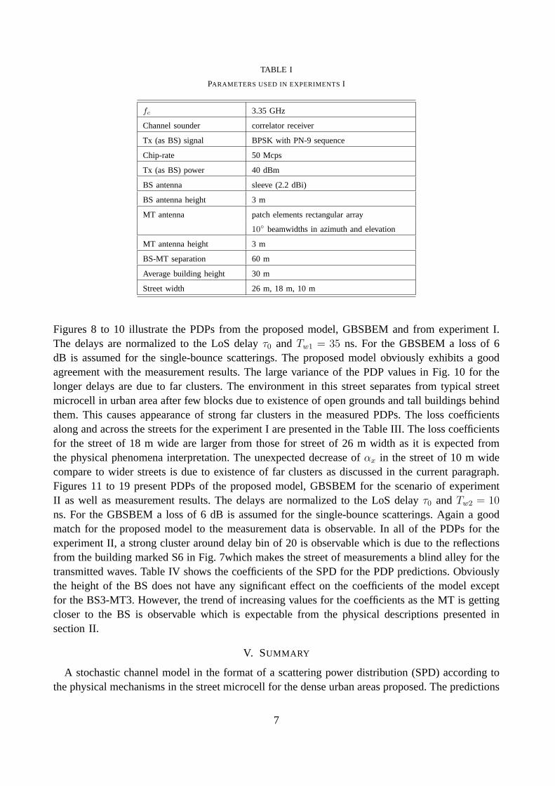
TABLE I

PARAMETERS USED IN EXPERIMENTSI

fc 3.35 GHz

Channel sounder correlator receiver

Tx (as BS) signal BPSK with PN-9 sequence

Chip-rate 50 Mcps

Tx (as BS) power 40 dBm

BS antenna sleeve (2.2 dBi)

BS antenna height 3 m

MT antenna patch elements rectangular array

10◦ beamwidths in azimuth and elevation

MT antenna height 3 m

BS-MT separation 60 m

Average building height 30 m

Street width 26 m, 18 m, 10 m

Figures 8 to 10 illustrate the PDPs from the proposed model, GBSBEM and from experiment I.The delays are normalized to the LoS delayτ0 and Tw1 = 35 ns. For the GBSBEM a loss of 6dB is assumed for the single-bounce scatterings. The proposed model obviously exhibits a goodagreement with the measurement results. The large varianceof the PDP values in Fig. 10 for thelonger delays are due to far clusters. The environment in this street separates from typical streetmicrocell in urban area after few blocks due to existence of open grounds and tall buildings behindthem. This causes appearance of strong far clusters in the measured PDPs. The loss coefficientsalong and across the streets for the experiment I are presented in the Table III. The loss coefficientsfor the street of 18 m wide are larger from those for street of 26 m width as it is expected fromthe physical phenomena interpretation. The unexpected decrease ofαx in the street of 10 m widecompare to wider streets is due to existence of far clusters as discussed in the current paragraph.Figures 11 to 19 present PDPs of the proposed model, GBSBEM for the scenario of experimentII as well as measurement results. The delays are normalizedto the LoS delayτ0 andTw2 = 10

ns. For the GBSBEM a loss of 6 dB is assumed for the single-bouncescatterings. Again a goodmatch for the proposed model to the measurement data is observable. In all of the PDPs for theexperiment II, a strong cluster around delay bin of 20 is observable which is due to the reflectionsfrom the building marked S6 in Fig. 7which makes the street ofmeasurements a blind alley for thetransmitted waves. Table IV shows the coefficients of the SPDfor the PDP predictions. Obviouslythe height of the BS does not have any significant effect on the coefficients of the model exceptfor the BS3-MT3. However, the trend of increasing values for the coefficients as the MT is gettingcloser to the BS is observable which is expectable from the physical descriptions presented insection II.

V. SUMMARY

A stochastic channel model in the format of a scattering power distribution (SPD) according tothe physical mechanisms in the street microcell for the dense urban areas proposed. The predictions

7

TABLE II

PARAMETERS USED IN EXPERIMENTSII

fc 5.2 GHz

Channel sounder RUSK DoCoMo

Tx (as BS) signal multitone

Bandwidth 100 MHz

Tx (as BS) power 40 dBm

BS antenna sleeve (2.2 dBi)

BS antenna height BS1=9.6 m, BS2=5.9 m, BS3=2.1 m

MT antenna patch elements cylindrical array

96 dual polarization port elements

MT antenna height 1.6 m

BS-MT horizontal separa-tion

MT1=59 m, MT2=30 m, MT3=21 m

Average building height 12 m

Street width 22 m (10.5 m)

Fig. 7. The scenario of experiment II.

of the proposed model for power-delay profiles (PDP) of the received signals compared to the dataobtained from two sets of measurements. The PDPs from the proposed model exhibits an excellentmatch to the experimental results, the azimuth-power spectrum (APS) were evaluated in [12] andpresented similar superior performance compared to the conventional models. The coefficients ofthe model were derived and compared for different street widths, BS antenna heights and BS-MTseparations. The loss coefficients increase as the BS-MT distance decreases and as the street widthdecreases, as it expected. No significant change in the loss coefficients due to the BS antennaheights were observed.

REFERENCES

[1] Y. Chen, V. Dubey, “Accuracy of geometric channel-modeling methods,”IEEE Trans. VT,Vol.53, No.1, pp. 82-93, Jan. 2004.

8

0 5 10 15 20 25 30 35−50

−40

−30

−20

−10

0

Nor

mal

ized

Rec

eive

d P

ower

[dB

]

Normalized Delay [(τ−τ0)/T

w1]

Measurement 1Measurement 2GBSBEMProposed

Fig. 8. The PDP from experiment I and predicted by the proposed model and GBSBEM. Street width=26 m.

0 5 10 15 20 25 30 35−50

−40

−30

−20

−10

0

Nor

mal

ized

Rec

eive

d P

ower

[dB

]


w1]

Measurement 1Measurement 2Measurement 3GBSBEMProposed


[2] W. Jakes,Microwave Mobile Communications, IEEE Press, 1974.[3] P. Petrus, J. Reed, T. Rappaport, “Geometrical-based statistical macrocell channel model for

mobile environments,”IEEE Trans. Comm., Vol.50, No.3, pp. 495-502, March 2002.[4] R. Janaswamy, “Angle and time of arrival statistics for the Gaussian scatter density model,”

IEEE Trans. Wireless Comm., Vol. 1, No. 3, pp. 488-497, July 2002.[5] T. Fujii, H. Omote, “Time-spatial path modeling for wideband mobile propagation,”VTC’04

Fall, Vol. 1, pp. 120-124, Sep. 2004.[6] T. Imai, T. Taga, “Statistical scattering model in urbanpropagation environment,”IEEE

Transactions on Vehicular Technology, Vol. 55, pp. 1081-1093, July, 2006.

9

0 5 10 15 20 25 30 35−50

−40

−30

−20

−10

0

Nor

mal

ized

Rec

eive

d P

ower

[dB

]


w1]

Measurement 1Measurement 2Measurement 3GBSBEMProposed


TABLE III

LOSSCOEFFICIENTS

Street Width [m] αx αy

26 8.0× 10−5

8.0× 10−4

18 1.0× 10−4

2.0× 10−3

10 7.0× 10−5

2.0× 10−3

[7] R. Ertel, P. Cardieri, K. Sowerby, T. Rappaport, J. Reed, “Overview of spatial channel modelsfor antenna array communication systems,”IEEE Pers. Comm. Mag., Vol. 5, No. 1, pp. 10 -22, Feb. 1998.

[8] J. Liberti, T. Rappaport, “A geometrically based model for line-of-sight multipath radiochannels,”VTC’96, Vol.2, pp. 844-848, May 1996.

[9] M. Lu, T. Lo, J. Litva, “A physical spatio-temporal modelof multipath propagation channels,”VTC 97, Vol. 2, pp. 810 - 814, May 1997.

[10] C. Oestges, V. Erceg, A. Paulraj, “A physical scatteringmodel for MIMO macrocellularbroadband wireless channels,”IEEE JSAC, Vol. 21, No. 5, pp. 721-729, June 2003.

[11] M. Marques, L. Correia, “A wideband directional channelmodel for UMTS microcells,”PIMRC’01, Vol. 1, pp. B-122-B-126, Sept. 2001.

[12] M. Ghoraishi, J. Takada, T. Imai, “A pseudo-geometrical channel model for dense urban line-of-sight street microcell,”Proceedings of the 17th Annual IEEE International Symposium onPersonal, Indoor and Mobile Radio Communications (PIMRC’06), Sept. 11-14, 2006 (Helsinki,Finland).

[13] Mir Ghoraishi, Junichi Takada, Tetsuro Imai, “Identification of Scattering Objects in MicrocellUrban Mobile Propagation Channel,”IEEE Transactions on Antennas and Propagation, Vol.54,No. 11, pp 3473-3480, Nov. 2006.

10

0 10 20 30 40 50−40

−30

−20

−10

0

Nor

mal

ized

Rec

eive

d P

ower

[dB

]


w2]

MeasurementGBSBEMProposed

Fig. 11. The measured PDP at experiment II, BS1-MT1, and PDPs predicted by the proposed model and GBSBEM.

0 10 20 30 40 50−40

−30

−20

−10

0

Nor

mal

ized

Rec

eive

d P

ower

[dB

]


w2]



TABLE IV

LOSSCOEFFICIENTS FORSCENARIO OFMEASUREMENT II

MT1 MT2 MT3

αx αy αx αy αx αy

BS1 1.0× 10−4

1.2× 10−3

1.7× 10−4

1.3× 10−3

1.7× 10−4

1.5× 10−3

BS2 1.0× 10−4

1.2× 10−3

1.7× 10−4

1.3× 10−3

1.7× 10−4

1.5× 10−3

BS3 1.0× 10−4

1.2× 10−3

1.7× 10−4

1.3× 10−3

0.5× 10−4

1.5× 10−3

11

0 10 20 30 40 50−40

−30

−20

−10

0

Nor

mal

ized

Rec

eive

d P

ower

[dB

]


w2]

MeasurementGBDBEMProposed


0 10 20 30 40 50−40

−30

−20

−10

0

Nor

mal

ized

Rec

eive

d P

ower

[dB

]


w2]



12

0 10 20 30 40 50−40

−30

−20

−10

0

Nor

mal

ized

Rec

eive

d P

ower

[dB

]


w2]



0 10 20 30 40 50−40

−30

−20

−10

0

Nor

mal

ized

Rec

eive

d P

ower

[dB

]


w2]



13

0 10 20 30 40 50−40

−30

−20

−10

0

Nor

mal

ized

Rec

eive

d P

ower

[dB

]


w2]



0 10 20 30 40 50−40

−30

−20

−10

0

Nor

mal

ized

Rec

eive

d P

ower

[dB

]


w2]



14

0 10 20 30 40 50−40

−30

−20

−10

0

Nor

mal

ized

Rec

eive

d P

ower

[dB

]


w2]



15

stochastic channel model for dense urban line-of … · stochastic channel model for dense urban...

Documents