stochastic approximation in monte carlo computation

Stochastic Approximation in Monte Carlo ComputationAuthor(s): Faming Liang, Chuanhai Liu and Raymond J. CarrollSource: Journal of the American Statistical Association, Vol. 102, No. 477 (Mar., 2007), pp.305-320Published by: American Statistical AssociationStable URL: http://www.jstor.org/stable/27639841 .

Accessed: 16/06/2014 09:43

Your use of the JSTOR archive indicates your acceptance of the Terms & Conditions of Use, available at .http://www.jstor.org/page/info/about/policies/terms.jsp

.JSTOR is a not-for-profit service that helps scholars, researchers, and students discover, use, and build upon a wide range ofcontent in a trusted digital archive. We use information technology and tools to increase productivity and facilitate new formsof scholarship. For more information about JSTOR, please contact [email protected].

.

American Statistical Association is collaborating with JSTOR to digitize, preserve and extend access to Journalof the American Statistical Association.

http://www.jstor.org

This content downloaded from 193.105.154.127 on Mon, 16 Jun 2014 09:43:35 AMAll use subject to JSTOR Terms and Conditions

http://www.jstor.org/action/showPublisher?publisherCode=astata

http://www.jstor.org/stable/27639841?origin=JSTOR-pdf

http://www.jstor.org/page/info/about/policies/terms.jsp


Stochastic Approximation in Monte Carlo Computation

Faming Liang, Chuanhai Liu, and Raymond J. Carroll

The Wang-Landau (WL) algorithm is an adaptive Markov chain Monte Carlo algorithm used to calculate the spectral density for a physical system. A remarkable feature of the WL algorithm is that it is not trapped by local energy minima, which is very important for systems

with rugged energy landscapes. This feature has led to many successful applications of the algorithm in statistical physics and biophysics; however, there does not exist rigorous theory to support its convergence, and the estimates produced by the algorithm can reach only a

limited statistical accuracy. In this article we propose the stochastic approximation Monte Carlo (SAMC) algorithm, which overcomes the

shortcomings of the WL algorithm. We establish a theorem concerning its convergence. The estimates produced by SAMC can be improved continuously as the simulation proceeds. SAMC also extends applications of the WL algorithm to continuum systems. The potential uses

of SAMC in statistics are discussed through two classes of applications, importance sampling and model selection. The results show that SAMC can work as a general importance sampling algorithm and a model selection sampler when the model space is complex.

KEY WORDS: Importance sampling; Markov chain Monte Carlo; Model selection; Spatial autologistic model; Stochastic approximation; Wang-Landau algorithm.

1. INTRODUCTION

Suppose that we are interested in sampling from a distribu tion that, for convenience, we write in the following form:

pix) = cpoix), xeX, (1)

where c is a constant and X is the sample space. As known

by many researchers, the Metropolis-Hastings (MH) sampler (Metropolis, Rosenbluth, Rosenbluth, Teller, and Teller 1953;

Hastings 1970) is prone to becoming trapped in local energy minima when the energy landscape of the distribution is rugged. [In terms of physics,

? log{/?n(x)} is called the energy func

tion of the distribution.] Over the last two decades, a various advanced Monte Carlo algorithms have been proposed to over

come this problem, based mainly on the following two ideas. The first idea is the use of auxiliary variables. Included in this

category are the Swendsen-Wang algorithm (Swendsen and

Wang 1987), simulated tempering (Marinari and Parisi 1992; Geyer and Thompson 1995), parallel tempering (Geyer 1991; Hukushima and Nemoto 1996), evolutionary Monte Carlo

(Liang and Wong 2001), and others. In these algorithms, the

temperature is typically treated as an auxiliary variable. Sim

ulations at high temperatures broaden sampling of the sample space and thus are able to help the system escape from local

energy minima.

The second idea is the use of past samples. The multicanon

ical algorithm (Berg and Neuhaus 1991) is apparently the first work in this direction. This algorithm is essentially a dynamic importance sampling algorithm in which the trial distribution is learned dynamically from past samples. Related works include the l//c-ensemble algorithm (Hesselbo and Stinchcombe 1995),

Faming Liang is Associate Professor, Department of Statistics, Texas A&M University, College Station, TX 77843 (E-mail: [email protected]). Chuanhai Liu is Professor, Department of Statistics, Purdue University, West

Lafayette, IN 47907 (E-mail: [email protected]). Raymond J. Carroll is Distinguished Professor, Department of Statistics, Texas A&M University, College Station, TX 77843 (E-mail: [email protected]). Liang's research was supported by grants from the National Science Foundation (DMS-04 05748) and the National Cancer Institute (CA104620). Carroll's research was

supported by a grant from the National Cancer Institute (CA57030) and by the Texas A&M Center for Environmental and Rural Health through a grant from the National Institute of Environmental Health Sciences (P30ES09106). The authors thank Walter W. Piegorsch, the associate editor, and three referees for their suggestions and comments, which led to significant improvement of this article.

the Wang-Landau (WL) algorithm (Wang and Landau 2001), and the generalized Wang-Landau (GWL) algorithm (Liang 2004, 2005). These differ from the multicanonical algorithm only in the specification and/or the learning scheme for the trial distribution. Other work included in this category is dynamic weighting (Wong and Liang 1997; Liu, Liang, and Wong 2001;

Liang 2002), where the acceptance rate of the MH moves is ad

justed dynamically with an importance weight that carries the information of past samples.

Among the algorithms described here, the WL algorithm has received much recent attention in physics. It can be de

scribed as follows. Suppose that the sample space X is fi nite. Let U(x) = ?

\og{po(x)} denote the energy function, let

{u\,..., um] be a set of real numbers containing all possible values of ?/(x), and let g(u) = #{x: U(x) ? u) be the number of states with energy equal to u. In physics, g(u) is called the

spectral density or the density of states of the distribution. For

simplicity, we also denote g(uj) by g? in what follows. The WL

algorithm is an adaptive Markov chain Monte Carlo (MCMC) algorithm designed to estimate g

= (g\,..., gm). Let g? be the

working estimate of g?. A run of the WL algorithm consists of several stages. The first stage starts with the initial estimates

?? j ? =

*gm = 1 and a sample drawn from X at random, and

iterates between the following steps:

The WL algorithm. 1. Simulate a sample x by a single Metropolis update with

the invariant distribution /?(x) oc \fg(U(x)). 2. Set g; ^-g^W(x)=M') for i = 1,..., m, where 8 is a gain

factor > 1 and /( ) is an indicator function.

The algorithm iterates until a flat histogram has been pro duced in the space of energy. Once the histogram is flat, the al

gorithm will restart by passing on ?>(w) as the initial value of the new stage and reducing 8 to a smaller value according to a pre

specified scheme, say, 8 <r- ^J~8. The process is repeated until 8

is very close to 1, say, log(5) < 10~8. Wang and Landau (2001) considered a histogram flat if the sampling frequency for each

energy value is not <80% of the average sampling frequency.

? 2007 American Statistical Association Journal of the American Statistical Association

March 2007, Vol. 102, No. 477, Theory and Methods DOI 10.1198/016214506000001202

305



306 Journal of the American Statistical Association, March 2007

Liang (2005) generalized the WL algorithm to continuum

systems. This generalization is mainly in terms of three re

spects: the sample space, the working function, and the estimate

updating scheme. Suppose that the sample space X is continu

ous and has been partitioned according to a chosen parameteri

zation, say, the energy function ?/(x), into m disjoint subregions denoted by E\ = {x: C/(x) < u\], E2 ? [x\u\ < i/(x) < u2), ..., Em-\

= {x:um-2 < Uix) <

um-\], and Em ?

{x: U(x) >

um-\], where u\,..., um-\ are m ? 1 specified real numbers.

Let \?f ix) be a nonnegative function defined on the sample space with 0 < fx\?/ix)dx<

oo. In practice, f(x) is often set to

po(x) defined in (1). Let g? = J?. t/t(x) ?fo. One iteration of GWL consists of the following steps:

The GWL algorithm. 1. Simulate a sample x by a number, k , of MH steps of which

the invariant distribution is defined as m . . .

pfxlaV^xGO. (2)

2. Set g>(X)+jt <-

g>(x)+* + oQk^gJ{x)+k for fc = 0, ..., m -

/(x), where 7(x) is the index of the subregion to which x belongs and q > 0 is a parameter that controls the sam

pling frequency for each of the subregions.

The extension of g? from the density of states to the integral

fE. Va (x) dx is of great interest to statisticians, because this leads to direct applications of the algorithm to model selection high est posterior density (HPD) region construction, and many other

Bayesian computational problems. Liang (2005) also studied the convergence of the GWL algorithm; as k becomes large, g? is consistent for g?. However, when k is small, say k = 1?the

choice adopted by the WL algorithm?there is no rigorous the

ory to support the convergence of g/. In fact, some deficiencies

of the WL algorithm have been observed in simulations. Yan and de Pablo (2003) noted that estimates of gi can only reach a

limited statistical accuracy that will not be improved with fur ther iterations, and the large number of configurations generated

toward the end of the simulation make only a small contribution to the estimates.

We find that this deficiency of the WL algorithm is caused by the choice of the gain factor 6. This can be explained as follows.

Let ns be the number of iterations performed in stage 5 and let os

be the gain factor used in stage s. Let n\ ? = ns = = n,

where n is large enough such that a flat histogram can be reached in each stage. Let logos

? ^ log?^-i decrease geomet

rically as suggested by Wang and Landau (2001). Then the tail sum n X^s+i l?g &s < ?? f?r any value of S. Note that the tail sum represents the total correction to the current estimate in the

iterations that follow. Hence the numerous configurations gen

erated toward the end of the simulation make only a small con

tribution to the estimates. To overcome this deficiency, Liang (2005) suggested that ns should increase geometrically with the rate log8s+\/log8s. However, this leads to an explosion in the total number of iterations required by the simulation.

In this article we propose a stochastic approximation Monte

Carlo (SAMC) algorithm, which can be considered a stochas tic approximation correction of the WL and GWL algorithms. In SAMC, the choice of the gain factor is guided by a condi tion given in the stochastic approximation algorithm (Andrieu,

Moulines, and Priouret 2005), which ensures that the estimates of g can be improved continuously as the simulation proceeds.

It is shown that under mild conditions, SAMC will converge. In addition, SAMC can bias sampling to some subregions of

interest, say the low-energy region, according to a distribution

defined on the subspace of the partition. This is different from

WL, where each energy must be sampled equally. It is also dif ferent from GWL, where the sampling frequencies of the sub

regions follow a certain pattern determined by the parameter ?.

Hesselbo and Stinchcombe (1995) and Liang (2005) showed

numerically that biasing sampling to low-energy regions often results in a simulation with improved ergodicity. This makes SAMC attractive for difficult optimization problems. In addi

tion, SAMC is user-friendly; it avoids the requirement of his

togram checking during simulations. We discuss the potential use of SAMC in statistics through two classes of examples: im

portance sampling and model selection. It turns out that SAMC can work as a general importance sampling method and a model

selection sampler when the model space is complex.

The article is organized as follows. In Section 2 we describe the SAMC algorithm and study its convergence theory. In Sec tion 3 we compare WL and SAMC through a numerical exam

ple. In Section 4 we explore the use of SAMC in importance sampling, and in Section 5 we discuss the use of SAMC in

model selection. In Section 6 we conclude the article with a

brief discussion.

2. STOCHASTIC APPROXIMATION MONTE CARLO

Consider the distribution defined in (1). For mathematical

convenience, we assume that X is either finite (for a discrete

system) or compact (for a continuum system). For a contin

uum system, X can be restricted to the region {x :po(x) > pm\n], where/?min is sufficiently small such that the region {x :po(x) <

Anin) is not of interest. As in GWL, we let E\,...,Em de

note m disjoint regions that form a partition of X. In practice, suPxeAf Po(x) is often unknown. An inappropriate specification of w/'s may result in that some subregions are empty. A sub

region Ej is empty if gi = fE, i?/(x) dx = 0. SAMC allows the

existence of empty subregions in simulations. Let gf denote the estimate of g? obtained at iteration t. For convenience, we

let Qti = log(gf}) and 0t = (0tU ..., 0tm). The distribution (2) can then be rewritten as

l m l ( \ PoM) -E ^7(x

G Ei), i = 1,..., m. (3) z=l

For theoretical simplicity, we assume that 0t e 0 for all t, where 0 is a compact set. In this article we set 0 = [-10100, 10100]m for all examples, although as a practical matter this is essentially equivalent to setting 0 = Rm. Because pot(x) is invariant with

respect to a location transformation of Gt?that is, adding to or

subtracting a constant vector from 0t will not change pot(x)?0t can be kept in the compact set in simulations by adjusting with a

constant vector. Because X and 0 are both assumed to be com

pact, an additional assumption is that pet(x) is bounded away from 0 and oo on X. Let the proposal distribution q(x, y) sat

isfy the following condition: For every xe X, there exist \ > 0 and 62 > 0 such that

|x-y|<6i =? q(x,y)>e2. (4)



Liang, Liu, and Carroll: Stochastic Approximation in Monte Carlo Computation 307

This is a natural condition in a study of MCMC theory (Roberts and Tweedie 1996). In practice, this kind of proposal can be

easily designed for both continuum and discrete systems. For a continuum system, g(x, y) can be set to the random-walk

Gaussian proposal y ~

N(x, a2/), with a2 calibrated to have a desired acceptance rate. For a discrete system, g(x, y) can be

set to a discrete distribution defined on a neighborhood of x by assuming that the states have been ordered in a certain way.

Let 71 = (7ZT,..., 7im) be an m-vector with 0 < iX[ < 1 and

Y^JLi^i ? 1> which defines the desired sampling frequency

for each of the subregions. Henceforth, ix is called the desired

sampling distribution. Let {yt} be a positive, nondecreasing se

quence satisfying oo oo

(a) 2_\ Yt ? oo and (b) >J y{ < oo (5) t=\ t=i

for some ? e (1, 2). For example, in this article we set

Y, =-??,

r=l,2,..., (6) max(?o, 0

for some specified value of io > 1. With the foregoing notation, one iteration of SAMC can be described as follows:

The SAMC algorithm. 1. Simulate a sample x(i+1) by a single MH update, of which

the proposal distribution is qix^\ ) and the invariant dis tribution ispotix).

2. Set 6>* = 0t + yi+i(ef+i -

n), where er+i =

(ef+i,i,...,

et+[,m) and et+\j = 1 if x^ e E? and 0 otherwise. If 0* e 0, then set 0t+[

= 0*\ otherwise, set 6t+\ = 0* + c*,

where c* = (c*,..., c*) can be an arbitrary vector that sat

isfies the condition 9* + c* e 0.

Remark. The explanation for condition (5) can be found in advanced books on stochastic approximation (e.g., Nevel'son

and Has'minskii 1973). The first condition is necessary for the convergence of 0t. If E??i Yt < ??> then, as follows from

step (b) (assuming that adjustment of 0t does not occur),

E~i I0H-U -

0ti\ < Er=i Yt\en ~

*i\ < E~i Yt < oo, where the second inequality follows from the fact 0 < etu ̂i S I Thus the value of 6ti does not reach log(g/) if, for example, the ini tial point Ooi is sufficiently far away from log(g?). On the other

hand, yt cannot be too large; an overly large yt will prevent

convergence. It turns out that the second condition in (5) as

ymptotically damps the effect of the random errors introduced

by et. When it holds, we have yt\eti ?

tt;| < Yt ?> 0 as t ?> 0.

SAMC falls into the category of stochastic approximation algorithms (Benveniste, M?tivier, and Priouret 1990; Andrieu et al. 2005). Theoretical results on the convergence of SAMC are given in the Appendix. The theory states that under mild

conditions, we have

Oh (L

C-r-logl / ifix)dx\-log?JTi + d) ifEi^i

?oo if ?7 = I

(7) as t -> 00, where d =

E/ {r?;=0} njlim ?

rno), mo is the num

ber of empty subregions, and C is an arbitrary constant. Because

pet ix) is invariant with respect to a location transformation of 0t, C cannot be determined by the samples drawn from pot (x). To

determine the value of C, extra information is needed; for exam

ple, J2?=\ e?tl is equal to a known number. Let nti denote the re alized sampling frequency of the subregion E? at iteration t. As t -+ oo, 7tti converges to n\ + d if E? / 0 and 0 otherwise. Note that for a nonempty subregion, the sampling frequency is inde

pendent of its probability, fE.p(x) dx. This implies that SAMC is capable of exploring the whole sample space, even for the

regions with tiny probabilities. Potentially, SAMC can be used to sample rare events from a large sample space. In practice, SAMC tends to lead to a "random walk" in the space of non

empty subregions (if each subregion is considered a "point") with the sampling frequency of each nonempty subregion be

ing proportional to 7r? + d. The subject area of stochastic approximation was founded

by Robbins and Monro (1951). After five decades of continual

development, it has developed into an important area in sys

tems control and optimization and has also served as a proto

type for the development of recursive algorithms for on-line estimation and control of stochastic systems. (See Lai 2003 for an overview.) Recently, it has been used with MCMC to solve maximum likelihood estimation problems (Younes 1988, 1999; Moyeed and Baddeley 1991 ; Gu and Kong 1998; Gelfand and Banerjee 1998; Delyon, Lavielle, and Moulines 1999; Gu and Zhu 2001). The critical difference between SAMC and other stochastic approximation MCMC algorithms lies in sam

ple space partitioning. With our use of partitioning, many new

applications can be established in Monte Carlo computation, for example, importance sampling and model selection, as de

scribed in Sections 4 and 5. In the same spirit, SAMC can also be applied to HPD interval construction, normalizing constant

estimation, and other problems, as discussed by Liang (2005). In addition, sample space partitioning improves its performance in optimization. Control of the sampling frequency effectively prevents the system from getting trapped into local energy min ima in simulations. We will explore this issue further elsewhere. It is noteworthy that Geyer and Thompson (1995) and Geyer (1996) mentioned that stochastic approximation can be used to determine the "pseudopriors" for simulated tempering (i.e., de

termining the normalizing constants of a sequence of distribu

tions scaled by temperature), although they provided no details. In Geyer's applications, the sample space is partitioned auto

matically according to the temperature variable.

For effective implementation of SAMC, several issues must be considered:

Sample space partition. This can be done according to our

goal and the complexity of the given problem. For exam

ple, if we aim to construct a trial density function for im

portance sampling (as illustrated in Sec. 4) or to minimize the energy function, then the sample space can be parti tioned according to the energy function. The maximum

energy difference in each subregion should be bounded by a reasonable number, say 2, to ensure that the local MH

moves within the same subregion have a reasonable ac

ceptance rate. Note that within the same subregion, sam

pling from the working density (3) is reduced to sampling from \?/ (x). If our goal is model selection, then the sample space can be partitioned according to the index of models, as illustrated in Section 5.




The desired sampling distribution. If we aim to estimate g, then we may set the desired distribution to be uniform, as is done in all examples in this article. However, if our goal is optimization, then we may set the desired distribution biased to low-energy regions. As shown by Hesselbo and Stinchcombe (1995) and Liang (2005), biasing sampling to low-energy regions often improves the ergodicity of the simulation. Our numerical results on BLN protein mod

els (Honeycutt and Thirumalai 1990) also strongly support this point. Due to space limitations, we will report these results elsewhere.

Choice of to and the number of iterations. To estimate g,

yt should be very close to 0 at the end of simulations. Oth

erwise, the resulting estimates will have a large variation.

The speed of yt going to 0 can be controlled by in. In prac tice, in can be chosen according to the complexity of the

problem. The more complex the problem, the larger the value of in that should be chosen. A large in will force the

sampler to reach all subregions quickly, even in the pres ence of multiple local energy minima. In our experience, in is often set to between 2m and 100m, with m being the number of subregions.

The appropriateness of the choice of to and the number of iterations can be determined by checking the convergence of

multiple runs (starting with different points) through examinat

ing for the variation of g or tt, where g and n denote the esti

mates of g and 71 obtained at the end of a run. A rough exam

ination for g is to check visually whether or not the g vectors

produced in the multiple runs follow the same pattern. Exis

tence of different patterns implies that the gain factor is still

large at the end of the runs, or that some parts of the sample

space are not visited in all runs. The examination for g" can also

be done by a statistical test under the assumption of multivari ate normality. (See Jobson 1992, pp. 150-153, for the testing

methods for multivariate outliers.)

To examine the variation of 5r, we define the statistic f(E?), which measures the deviation of 777, the realized sampling fre

quency of subregion E[ in a run, from its theoretical value. The statistic is defined as

f(Ei) :

TCi ?

(71/ + d) -^? x 100% if E; is visited /Cx

0 otherwise,

for / = 1, . . . , m, Where 2 =

?^{/:/r. is not visited} *j/(m

- m'o)

and mf0

is the number of subregions that are not visited. Note

that d can be considered an estimate of d in (7). It is said that

{ f(Ei)}9 output from all runs and for all subregions, matches well if the following two conditions are satisfied: (a) There does not exist such a subregion that is visited in some runs but not in others, and (b) max ^ \ef(E?)\ is less than a threshold value, say 10%, for all runs. A group of {e/(E;)} that does not match

well implies that some parts of the sample space are not vis

ited in all runs, in is too small (the self-adjusting ability is thus

weak), or the number of iterations is too small. We note that the

idea of monitoring convergence of MCMC simulations using multiple runs was discussed by Gelman and Rubin (1992) and

Geyer (1992). In practice, to have a reliable diagnostic for the convergence,

we may check both g and n. In the case where a failure of

multiple-run convergence is detected, SAMC should be rerun with more iterations or a larger value of to. Determining io and

the number of iterations is a trial-and-error process.

3. TWO DEMONSTRATION EXAMPLES

Example 1. In this example we compare the convergence and

efficiency of the WL and SAMC. The distribution of the exam

ple consists of 10 states with the unnormalized mass function

Pix) as given in Table 1. It has two modes that are well sepa rated by low-mass states.

The sample space was partitioned according to the mass

function into the following five subregions: E\ = {8}, E2 ?

{2}, E3 = {5,6}, E4 = {3,9}, and E5 = {1,4,7,10}. In sim

ulations, we set V ix) = 1. The true value of g is then g =

(1, 1, 2, 2, 4), which is the number of states in the respective subregions. The proposal used in the MH step is a stochas tic matrix of which each row is generated independently from the Dirichlet distribution Dir il,..., 1). The desired sampling distribution is uniform, that is, n\ = = tt^

? 1/5. The se

quence {yt} is as given in (6) with to = 10. SAMC was run for 100 times independently. Each run consists of 5 x IO5 it erations. The estimation error of g was measured by the func

tion eit) = y Es^f?/0 -

gi)2/gi at 10 equally spaced time

points, t = 5 x IO4,..., 5 x 105. Figure 1(a) shows the curve

of eeit) obtained by averaging over the 100 runs. The statistic

/ (?;) was calculated at time t = 105 for each run. The results show that they match well. Figure 1(b) shows boxplots of the

e/(E?)'s of the 100 runs. The deviations are <3%. This indicates that SAMC has achieved the desired sampling distribution and the choice of io and the number of iterations are appropriate. Other choices of to, including to = 20 and 30, were also tried, and the results were similar.

We applied the WL algorithm to this example with the same

proposal distribution as that used in SAMC. In the runs, the gain factor was set as done by Wang and Landau (2001); it started with ?o = 2.718 and then decreased in the scheme 8s+\ -> y/8?. Let ns denote the number of iterations performed in stage s. For

simplicity, we set ns to a constant that was large enough such

that a flat histogram can be formed in each stage. The choices of

ns that we tried included ns = 1,000, 2,500, 5,000, and 10,000. The estimation error was also measured by ee(t) evaluated at

t = 5 x IO4,..., 5 x 105, where t is the total number of itera

tions made so far in the run. Figure 1(a) shows the curves of

eit) for each choice of ns, where each curve was obtained by

averaging over 100 independent runs.

The comparison shows that for this example, SAMC pro duces more accurate estimates for g and converges much faster

than WL. More importantly, in SAMC the estimates can be im

proved continuously as the simulation proceeds, whereas in WL

the estimates can reach only a certain accuracy depending on

the value ofns.

Example 2. As pointed out by Liu (2001), umbrella sam

pling (Torrie and Valleau 1977) can be seen as a precursor of

Table 1. The Unnormalized Mass Function of the 10-State Distribution

x 1 234567 89 10 P(x) 1 100 2 1 3 3 1 200 2 1



Liang, Liu, and Carroll: Stochastic Approximation in Monte Carlo Computation

(a)

309

S3 d

S3 ?

d

d

o d

t.H.H-.*.+.*.t.*

A-?to?4^-??+???f?J?*

L

CM H

?

? ^

f f

100000 200000 300000 400000 500000 ? Numbered energy evaluations subregions

Figure 1. Comparison of the WL and SAMC Algorithms, (a) Average e(t) curves obtained by SAMC and WL. The vertical bars show the ? ) standard deviation of the average of the estimates (-SAMC;.WL, n = 1,000;-WL, n = 2,500;-WL, n = 5,000;-WL, n = 10,000). (b) Boxplots of { f(E,)} obtained in 100 runs of SAMC.

many advanced Monte Carlo algorithms, including simulated

tempering, multicanonical, and thus WL, GWL, and SAMC.

Although umbrella sampling was proposed originally for esti

mating the ratio of two normalizing constants, it also can be used as a general importance sampling method. Recall that the basic idea of umbrella sampling is to sample from an "umbrella distribution" (i.e., a trial distribution in terms of importance sampling), which covers the important regions of both target distributions. Torrie and Valleau (1977) proposed two possible schemes for construction of umbrella distributions. One is to

sample intermediate systems of the temperature-scaling form

pS}(x) a [po(x)]l/Ti for Tm > Tm-\ > > T\ = 1. This leads

directly to the simulated tempering algorithm. The other one is to sample a weighted distributionpu(x) oc co{U(x)}po(x), where the weight function co(-) is a function of the energy variable and can be determined by a pilot study. Thus umbrella sampling can be seen as a precursor of multicanonical, WL, GWL, and

SAMC. Sample space partitioning, motivated by discretization of continuum systems, provides a new methodology for apply ing umbrella sampling to continuum systems. Although SAMC and simulated tempering both fall in the

class of umbrella sampling algorithms, they have quite different

dynamics. This can be illustrated by an example. The distribu tion is defined as p(x) oc e~U(-x\ where x e [?1.1, l.l]2 and

?/(x) = ~{x\ sin(20jc2) + JC2sin(20jci)}2cosh{sin(10jci)xi} -

{jci cos(10x2) ?

X2sin(10jci)}2cosh{cos(20;c2)JC2}. This exam

ple is modified from example 5.3 of Robert and Casella

(2004). Figure 2(a) shows that ?/(x) has a multitude of lo cal energy minima separated by high-energy barriers. When

applying SAMC to this example, we partitioned the sample space into 41 subregions with an equal energy bandwidth, Ei = {x: i/(x) < -8.0}, E2 = {x: -8.0 < t/(x) < -7.8}, and ?41 = {x: ?.2 < ?/(x) < 0}, and set other parameters as follows: V(x) = e~U(x\ t0 = 200, n\ = = tt4i = 1/41, and a random-walk proposal, qixtt ) = N2(x,, .252I2). SAMC was run for 20,000 iterations, and 2,000 samples were collected at

equally spaced time points. Figure 2(b) shows the evolving path of the 2,000 samples. For comparison, MH was applied to sim ulate from the distribution pstix) oc e~u(x)/5, MH was run for

20,000 iterations with the same proposal N2ixt, .252I2), and

2,000 samples were collected at equally spaced time points. Figure 2(c) shows the evolving path of the 2,000 samples, which characterizes the performance of simulated tempering at high temperatures.

The result is clear. In the foregoing setting, SAMC samples almost uniformly in the space of energy [i.e., the energy band width of each subregion is small, and the sample distribution

closely matches the contour plot of t/(x)], whereas simulated




-1.0 -0.5 0.0 0.5 1.0

Figure 2. (a) Contour of U(x), (b) Sample Path of SAMC, and (c) Sample Path of MH.

tempering tends to sample uniformly in the sample space X when the temperature is high. Because we usually do not know where the high-energy and low-energy regions are and how much the ratio of their "volumes" is a priori, we cannot control the simulation time spent on low-energy and high-energy re

gions in simulated tempering. However, we can control almost

exactly, up to the constant d in (7), the simulation time spent on

low-energy and high-energy regions in SAMC by choosing the desired sampling distribution n. SAMC can go to high-energy regions, but it spends only limited time there to help the sys tem to escape from local energy minima, and also spends time

exploring low-energy regions. This smart simulation time dis tribution scheme makes SAMC potentially more efficient than simulated tempering in optimization. Due to the space limita

tions, we do not explore this point in this article. But we note that Liang (2005) reported a neural network training example in which it was shown GWL is more efficient than simulated

tempering in locating global energy minima.

4. USE OF STOCHASTIC APPROXIMATION MONTE CARLO IN IMPORTANCE SAMPLING

In this section we illustrate the use of SAMC as an impor tance sampling method. Suppose that because of its rugged en

ergy landscape, the target distribution /?(x) is very difficult to simulate from with conventional Monte Carlo algorithms. Let

xi,..., xn denote the samples drawn from a trial density /?*(x), and let wi,..., wn denote the associated importance weights, where w? =p(x,-)/p*(X|) for i = 1,..., n. The quantity Ephix) then can be estimated by

?^)=^J^l. (9) Although this estimate converges almost surely to Eph(x), its variance is finite only if

Ep*h2ix)(^)2dx= f h\x)P^dx <oo.

\p*ix)J Jx />*(*) If the ratio p(x)//?*(x) is unbounded, then the weight /?(x?)/ p*ix?) will vary widely, and thus the resulting estimate will be unreliable. A good trial density should necessarily satisfy the

following two conditions:

a. The importance weight is bounded; that is, there exists a number M such that/?(x)/p*(x) < M for all x X.

b. The trial density /?*(x) can be easily simulated from using conventional Monte Carlo algorithms.




In addition, the trial density should be chosen to have a similar

shape to the true density. This will minimize the variance of the resulting importance weights. Of course, how to specify an

appropriate trial density for a general distribution has been a

long-standing and difficult problem in statistics. The defensive mixture method (Hesterberg 1995) suggests

the following trial density:

p*(x) = Xp(x) + (\-\)p(x), (10)

where 0 < X < 1 and p(x) is another density. However, in prac tice, p*(x) is rather poor. Although the resulting importance weights are bounded above by 1/?, it cannot be easily sam

pled from using conventional Monte Carlo algorithms. Because

p*(x) contains p(x) as a component, if we can sample from

p*(x), then we can also sample from p(x). In this case we do

not need to use importance sampling! Stavropoulos and Titter

ington (2001), Warnes (2001), and Capp?, Giullin, Marin, and Robert (2004) suggested constructing the trial density based on

previous Monte Carlo samples, but the trial densities result

ing from their methods cannot guarantee that the importance

weights are bounded. We note that these methods are similar to

SAMC in the spirit of learning from historical samples. Other trial densities based on simple mixtures of normals or t distri butions also may result in unbounded importance weights, al

though they can be sampled from easily. Suppose that the sample space has been partitioned accord

ing to the energy function, and that the maximum energy dif ference in each subregion has been bounded by a reasonable number such that the local MH move within the same subre

gion has a reasonable acceptance rate. It is then easy to see that

the distribution defined in (2) or (3) satisfies the foregoing two conditions and can work as a universal trial density even in the

presence of multiple local minima on the energy landscape of the true density. Let

^ v^ w(x) p00(x)cxT^r?I(xeEl) (11)

ti Si denote the trial density constructed by SAMC with \j/(x) =

Po(x), where g; =

lim^oo e9ti. Assuming that^- has been nor

malized by an additional constraint (e.g., ̂A=\Si *s a known

constant), the importance weights are then bounded above by

max^j *gi < Jx ir(x) dx < oo. As shown in Section 2, sampling from j?oo(x) will lead to a "random walk" in the space of non

empty subregions. Hence the whole sample space can be well

explored. Besides satisfying the conditions (a) and (b), Poo(x) has two

additional advantages over other trial densities. First, the simi

larity of the trial density to the target density can be controlled to some extent by the user. For example, instead of ( 11), we can

sample from the following density:

to(x)ay^/(x6?,), (12) t?x^

where the parameters Xl-, i = 1,..., m, control the sampling fre

quency of the subregions. Second, resampling can be made on

line if we are interested in generating equally weighted samples from p(x). Let coi = gz/max^j g) denote the resampling prob ability from the subregion ?;, and xt denote the sample drawn

from poo (x) at iteration t. The resampling procedure consists of the following three steps:

The SAMC importance-resampling algorithm. 1. Draw a sample xr ^/?oo(x) using a conventional Monte

Carlo algorithm, say, the MH algorithm. 2. Draw a random number U ?

uniform(0, 1). If U < cok,

then save xr as a sample of p(x), where k is the index of the subregion xr belongs to.

3. Set t <<? t + 1 and go to step 1, until sufficient samples have been collected.

Consider the following distribution:

pix) = ^N

1

-N

-N

1 -0.9

1 0 0 1

-.9

which is identical to that given by Gilks, Roberts, and Sahu

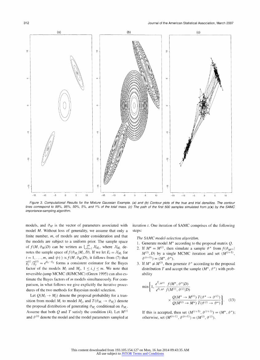
(1998), except that the mean vectors are separated by a larger distance in each dimension. Figure 3(a) shows its contour

plot, which contains three well-separated components. The MH

algorithm has been used to simulate fromp(x) with a random walk proposal N(x, I2), but it failed to mix the three compo nents. However, an advanced MCMC sampler, such as sim

ulated tempering, parallel tempering, or evolutionary Monte

Carlo, should work well for this example. Our purpose in study ing this example was just to illustrate how SAMC can be used in

importance sampling as a universal trial distribution constructor

and how SAMC can be used as an advanced sampler to sample from a multimodal distribution. We applied SAMC to this example with the same proposal as

used in the MH algorithm. Let X = [-10100, IO100]2 be com

pact. It was partitioned with an equal energy bandwidth Au = 2 into the following subregions: E\ = {x:

? log/?(x) < 0}, E2 ?

{x : 0 < -

logpix) < 2}, ..., and En = {x : -

logp(x) > 20}. Set i^(x) =/?(x), to ? 50 and the desired sampling distribution to be uniform. In a run of 500,000 iterations, SAMC produced a trial density with the contour plot as shown in Figure 3(b). On the plot there are many contour circles formed due to the den

sity adjustment by g/'s. The adjustment means that many points of the sample space have the same density value. The SAMC

importance-sampling algorithm was then applied to simulate

samples from pix). Figure 3(c) shows the sample path of the first 500 samples generated by the algorithm. All three compo nents had been well mixed. Later, the run was lengthened, and

the mean and variance of the distribution were estimated ac

curately using the simulated samples. The results indicate that SAMC can indeed work as a general trial distribution construc tor for importance sampling and an advanced sampler for sim

ulation from a multimodal distribution.

5. USE OF STOCHASTIC APPROXIMATION MONTE CARLO IN MODEL SELECTION PROBLEMS

5.1 Algorithms

Suppose that we have a posterior distribution denoted by /(M, #a/|D), where D denotes the data, M is the index of




(a)

Figure 3. Computational Results for the Mixture Gaussian Example, (a) and (b) Contour plots of the true and trial densities. The contour lines correspond to 99%, 95%, 50%, 5%, and 1% of the total mass, (c) The path of the first 500 samples simulated from p(x) by the SAMC

importance-sampling algorithm.

models, and ?m is the vector of parameters associated with

model M. Without loss of generality, we assume that only a

finite number, m, of models are under consideration and that

the models are subject to a uniform prior. The sample space

of f(M, &m\D) can be written as U?=i ^m?, where Xm? de notes the sample space of f(UM? Wi, D). If we let E? = Xm? for / = 1,..., ra, and \?/(-) ex f(M, ?M\D), it follows from (7) that

g: fg- = eeti~6tJ forms a consistent estimator for the Bayes

factor of the models M; and My, 1 < i,j < m. We note that

reversible-jump MCMC (RJMCMC) (Green 1995) can also es

timate the Bayes factors of m models simultaneously. For com

parison, in what follows we give explicitly the iterative proce dures of the two methods for Bayesian model selection.

Let Q(Mi -> Mj) denote the proposal probability for a tran

sition from model Mz to model My, and T(um? ~^ &M-) denote

the proposal distribution of generating ?mj conditional on ?m? Assume that both Q and T satisfy the condition (4). Let M^ and ?(r) denote the model and the model parameters sampled at

iteration t. One iteration of SAMC comprises of the following steps:

The SAMC model-selection algorithm. 1. Generate model M* according to the proposal matrix Q. 2. If M* = M(f), then simulate a sample #* from/(#M(o|

M(r),D) by a single MCMC iteration and set (M(r+1), #('+!)) = (M*,#*).

3. If M* 7^ Mw, then generate ?* according to the proposal distribution T and accept the sample (M*, #*) with prob ability

f e*M{t) fiM*,?*\D) mm { 1, ?a-?-?

\ ee<M* fiM?\?^\D)

QjM^M^Tj?*-*^)] x ?(M^ -> m*) r(#w ->#*) J

'

If this is accepted, then set (M(r+1), #(r+1)) = (M*, #*); otherwise, set (M(m), ??+V) = (M(?), #(0).




4. Set 0* =9t + yr+i(e,+ 1 -

7r), where er+! =

(er+u,...,

^i+i,m) and et+\,i = 1 if M(r+1) = M? and 0 otherwise. If 69* g 0, then set 0t+\

= #*; otherwise, set 0t+\

= 0* + c*,

where c* is chosen such that 6* + c* G 0.

Let S;(r) = #{M(/:) = Mi : A; = 1, 2,..., t] be the sampling fre

quency of model Mz during the first ? iterations in a run of RJMCMC. With the same proposal matrix Q, the same proposal distribution T and the same MH step (or Gibbs cycle) as those used by SAMC, one iteration of RJMCMC can be described as

follows:

The RJMCMC algorithm. 1. Generate model M* according to the proposal matrix Q. 2. If M* = M(r), then simulate a sample ?* from f(?M(o\

M{?\D) by a single MCMC iteration and set (M(r+1), #('+1)) = (M*,#*).

3. If M* 7^ M^\ then generate ?* according to the proposal density T and accept the sample (M*, ?*) with probabil ity

. f /(M*,iT|D) min< 1,-?-? I /(Mtt,#(f)|D)

?(M* -> M(i)) r(#* -> #(i)) 1 x

?(M^) -> M*) T(^W -> #*) J '

If it is accepted, then set (M(r+1), #(i+1)) = (M*,#*); otherwise, set (M(r+1), #(r+1)) = (M(t\ Mf)).

4. Set Sf+1) =

sf)+/(M(i+1)=Ml-)for/= l,...,m.

The standard MCMC theory (Tierney 1994) implies that as

t -> oo, 3Z 7 3 forms a consistent estimator for the Bayes

factor of model M, and model My. We note that the form of the RJMCMC algorithm just de

scribed is not the most general one, where the proposal dis

tribution T(- -> ) is assumed such that the Jacobian term in

(14) is reduced to 1. This observation is also applicable to the SAMC model-selection algorithm. The MCMC algorithm used in step 2 of the foregoing two algorithms can be the MH al

gorithm, the Gibbs sampler (Geman and Geman 1984), or any other advanced MCMC algorithms, such as simulated temper

ing, parallel tempering, evolutionary Monte Carlo, and SAMC

importance-resampling (discussed in Sec. 3). When the distri

bution/(M, ?m\D) is complex, an advanced MCMC algorithm may be chosen and multiple iterations may be used in this step.

SAMC and RJMCMC are different only at steps 3 and 4, that is, in the manner of acceptance for a new sample and esti

mation for the model probabilities. In SAMC, a new sample is accepted with an adjusted probability. The adjustment al

ways works in the reverse direction of the estimation error of

the model probability or, equivalently, the frequency discrep ancy between the realized sampling frequency and the desired one. Thus it guarantees convergence of the algorithm. In sim

ulations, we can see that SAMC can overcome any difficulties

in dimension-jumping moves and provide a full exploration for all models. Recall that the proposal distributions have been as

sumed to satisfy the condition (4). Because RJMCMC does not

have the self-adjusting ability, it samples each model in a fre

quency proportional to its probability. In simulations, we can see that RJMCMC often stays on a model for a long time if that

model has a significantly higher probability than its neighbor ing models. In SAMC, the estimates of the model probabilities are updated in the logarithmic scale; this makes it possible for SAMC to work for a group of models with huge differences in

probability. This is beyond the ability of RJMCMC, which can

work only for a group of models with comparable probabilities. Finally, we point out that for a problem that contains only

several models with comparable probabilities, SAMC may not

be better than RJMCMC, because in this case its self-adjusting ability is no longer crucial for mixing of the models. SAMC is essentially an importance sampling method (i.e., the samples are not equally weighted); hence its efficiency should be lower than that of RJMCMC for a problem in which RJMCMC suc

ceeds. In summary, we suggest using SAMC when the model

space is complex, for example, when the distribution fiM\D) has well-separated multiple modes or when there are probabil

ity models that are tiny but of interest to us.

5.2 Numerical Results

The autologistic model (Besag 1974) has been widely used for spatial data analysis (see, e.g., Preisler 1993; Augustin,

Mugglestone, and Buckland 1996). Let s = {si :i G D] denote a configuration of the model in which the binary response Si e {?1, +1} is called a spin and D is the set of indices of the spins. Let \D\ denote the total number of spins in D, and let Nii) denote a set of the neighbors of spin /. The probability

mass function of the model is

Ty MJ l ieD ieD JeN(i) 7 J

ia,?)eQ, (15)

where Q is the parameter space and cpia, ?) is the normalizing constant defined by

(pia,?)= Yl exP \aJlSi+2^ Si

for all possible s l ieD ieD yjeN(i)

The parameter a determines the overall proportion of s? with a

value of +1, and the parameter ? determines the intensity of the interaction between s? and its neighbors.

A major difficulty with this model is that the function cpia, ?) is generally unknown analytically. Evaluating cpia, ?) exactly is prohibitive even for a moderate system, because it requires

summary over all 2'D' possible realizations of s. Because

cpia, ?) is unknown, importance sampling is perhaps the most

convenient technique if we aim at calculating the expectation

Ea.?his) over the parameter space. This problem is a little dif ferent than conventional importance sampling problems dis

cussed in Section 4, where we have only one target distribution, whereas here we have multiple target distributions indexed by their parameter values. A natural choice for the trial distribution is a mixture distribution of the form

I m*

pS?x(s) = ^tE^sI^?')' (16)

7=1

where the values of the parameters ia\, ?\),..., (am*, ?m*) are prespecified. We note that this idea has been suggested



314

O CO

O

o

o CO

o CM

o J

Journal of the American Statistical Association, March 2007

(b) CD

O m

o

o CO

o CM

o J

20 40 60 20 40 60

Figure 4. U.S. Cancer Mortality Rate Data, (a) The mortality map of liver and gallbladder cancer (including bile ducts) for white males during the decade 1950-1959. The black squares denote the counties of high cancer mortality rate, and the white squares denote the counties of low cancer mortality rate, (b) Fitted cancer mortality rates. The cancer mortality rate of each county is represented by the gray level of the corresponding square.

by Geyer (1996). To complete this idea, the key is to esti mate

(p(cij, ?j),..., (p(otm*,?m*). The estimation can be up to

a common multiplicative constant that will be canceled out in calculation of Ea^h(s) in (9). Geyer (1996) also suggested stochastic approximation as a feasible method for simultane

ously estimating (p(ci\, ?\),..., (p(um*,?m*), but gave no de

tails. Several authors have based their inferences for a distri bution like (15) on the estimates of the normalizing constant function at a finite number of points. For example, Diggle and Gratton (1984) proposed estimating the normalizing constant function on a grid, smoothing the estimates using a kernel

method, and then substituting the smooth estimates into (15) as known for finding maximum likelihood estimators (MLEs) of the parameters. A similar idea was also been proposed by Green and Richardson (2002) for analyzing a disease-mapping example.

In this article we explore the idea of Geyer (1996) and give details about how SAMC can be used to simultaneously es timate (p(ct\, ?\),..., (p(am*,?m*) and how the estimates can

be further used in estimation of the model parameters. The dataset considered is the U.S. cancer mortality rate, as shown in Figure 4(a). Following Sherman, Apamasovich, and Carroll

(2006), we modeled the data by a spatial autologistic model. The total number of spins is |D| =2,293. Suppose that the para meter points used in (16) form a 21 x 11 lattice (m* = 231) with a equally spaced between ?.5 and .5 and ? between 0 and .5. Because (pia, ?) is a symmetric function about a, we only need to estimate it on a sublattice with a between 0 and .5. The sub lattice consists of m = 121 points. Estimating the quantities ^(?i, ?\),.. , <piotm, ?m) can be treated as a Bayesian model selection problem, although no observed data are involved. This is because (p(ct\,?\),..., (piotm, ?m) correspond to the normal

izing constants of different distributions. In what follows, the S AMC model-selection algorithm and the RJMCMC algorithm were applied to this problem by treating each grid point (a/, ?j) as a different model andp(s|a/, ?j)<p(cij, ?j) as the posterior dis tribution used in (13) and (14).

SAMC was first applied to this problem. The proposal ma

trix g, the proposal distribution 7\ and the MCMC sampler used in step 2 are specified as follows. Let the m models be coded as a matrix (Af,y) with / = 0,..., 10 and j = 0,..., 10. The proposal matrix Q is then defined as

Q(M9^Mff) = q%>q$>,




where $>_,

= 9g>

= q%

= 1/3 for i = 1,.... 9, *?g =

9g10 = 2/3, and ^

= q 9 = 1/3; and ?^, =

c/ff =

A, = 1/3 for /= 1,.... 9, 9$

= ?(,g10

= 2/3, and q =

q^9 = 1/3. For this example, ? corresponds to the configu

ration s of the model. The proposal distribution T(?^ -? #*) is an identical mapping, that is, keeping the current configu ration unchanged when a model is proposed to be changed to another one. Thus we have T(?(t) -> ?*) = T(?* -> ?{t)) = 1. The MCMC sampler used in step 2 is the Gibbs sampler (Ge man and Geman 1984), sampling spin / from the conditional distribution

p(Si = +i |iv(o) = ?z??ET?7)> (17)

P(si = -1 \N(i)) = 1 - P(S? = +1 \N(i)),

for all i G D in a prespecified order. SAMC was run five times independently. Each run consisted

of two stages. The first stage estimated the function cp(a, ?) on

the sublattice. In this stage, SAMC was run with in = 104 and for 108 iterations. The second stage drew importance samples from the trial distribution,

1 m* 1 m*

?^<p((Xk,?k)

xexpUkJ2Si + Y^Si\ ^ Sj)l (18)

* ieD ieD \eN(i) ' '

which represents an approximation to (16), with (p(a.j,?j) re

placed by its estimate obtained in the first stage. In this stage SAMC was run with 8t

= 0 and for 107 iterations, and a total of

105 samples were harvested at equally spaced time points. Each run cost about 115 minutes of CPU time in a 2.8-GHz computer. In the second stage, SAMC is reduced to RJMCMC by setting 8t = 0. Figure 5(a) shows one estimate of (p(a, ?) obtained in a run of SAMC.

Using the importance samples collected earlier, we estimated

the probability P(s? = +l|a, ?), which is a function of (a, ?). The estimation can be done in (9) by setting h(s) ? J2ieD^si +

1)/(2|D|). By averaging over the five runs, we obtained one

estimate of the function, as shown in Figure 5(b). To assess the variation of the estimate, we calculated the standard deviation

of the estimate at each grid point of the lattice. The average of the standard deviations is 3 x 10-4. The estimate is fairly stable.

Using the importance samples collected earlier, we also esti

mated the parameters ia, ?) for the cancer data shown in Fig ure 4(a). The estimation can be done using the Monte Carlo maximum likelihood method (Geyer and Thompson 1992;

Geyer 1994) as follows. Let p*(s) ?

c*/?q(s) denote an ar

bitrary trial distribution for (15), where p^is) is completely specified and c* is an unknown constant. Let i/>(a, ?,s) =

cpia, ?)pis\a, ?) and let Lia, ?\s) denote the log-likelihood function of an observation s. Thus

Ln(a,?\s)

iogi -

> ;r vt:;~ /1 m 1 "xl/ia,?,s(k)) "^ P%i*{k)) k=\

(1) M are approaches Lia, ?\s) as n -> oo, where s1

MCMC samples simulated from p*(s). The estimate (a,

?) ?

argmaxa)jgLn(a, )?|s) is called the Monte Carlo MLE

(MCMLE) of ia, ?). The maximization can be done using a

conventional optimization procedure, say the conjugate gradi

ent method. Setting p*(s) =/%lix(s), the five runs of SAMC resulted in five estimates of ia, ?). The mean and standard de viation vectors of these estimates were (?.2994, .1237) and

(.00063, .00027). Henceforth, these estimates are called mix

MCMLEs, because they are obtained based on a mixture trial distribution. Figure 4(b) shows the fitted mortality map based on one mix-MCMLE (-.2999, .1234).

In the literature, p*(s) is often constructed based on a single parameter point, that is, setting

p*(s) oc expL* J^si + y X>( Y sj) f ' (20)

ieD ieD

(a) (b)

Figure 5. Computational Results of SAMC. (a) Estimate of logy (c?, ?) on a 21 x 11 lattice with a {-.5, -.45, ..., .5} and ? e {0, .05, ..., .5}.

(b) Estimate of P(s? = + 11a, ?) on a 50 x 25 lattice with a e {-.49, -.47, ..., .49} and ? e {.01, .03, ..., .49}.




where (a*, ?*) denotes the parameter point. The point (o?*, ?*) should be chosen to be close to the true parameter point; other

wise, a large value of n would be required for the convergence of (19). Sherman et al. (2006) set (a*, ?*) to be the maximum

pseudolikelihood estimate (Besag 1975) of (a, ?), which is the MLE of the pseudolikelihood function

PL(a,j8|s)

_i-r_expfai? +

?lljeNioSj)}_ " JeD eXp{a + ? ?/ *(0 SJ} + exP{~a

- ? T,jeN(i) sj} '

(21)

We repeated the procedure of Sherman et al. for the cancer data five times with n = 105 and the MCMC samples collected at

equally spaced time points in a run of the Gibbs sampler of 107 iteration cycles. The mean and standard deviation vectors of the

resulting estimates are (-.3073, .1262) and (.00837, .00946). These estimates have a significantly higher variation than the mix-MCMLEs. Henceforth, these estimates are called single MCMLEs, because they are obtained based on a single-point trial distribution.

To compare the accuracy of the mix-MCMLEs and single MCMLEs, we conducted the following experiment based on the

principle of the parametric bootstrap method (Efron and Tibshi rani 1993). Let T, =

E,eD*/ and T2 = \ E?6WE,eW) sj). It is easy to see that T = (Ti, T2) forms a sufficient statistic of (a, ?). Given an estimate (c?, ?), we can reversely estimate

Table 2. Comparison of the Accuracy of the Mix-MCMLEs and

Single-MCMLEs for the U.S. Cancer Data

Estimate Single-MCMLE Mix-MCMLE

RMSE(t'im) 59.51 2.90

RMSE(t2im) 114.91 4.61

NOTE: RMSE(tfm) is calculated as ^ELi (tf"'* -*?bs)2/5, where /' = 1,2, and tf",fc denotes

the value of tfm calculated based on the frth estimate of (a, ?).

the quantities Ti and T2 by drawing samples from the dis

tribution/(s|a, ?). If (a, ?) is accurate, then we should have

tobs ̂ tsim? where tobs and tsim denote me yalues of T caku_ lated from the true observation and from the simulated sam

ples. To calculate tsim, we generated 1,000 independent config urations conditional on each estimate, with each configuration generated by a short run of the Gibbs sampler. The Gibbs sam

pler started with a random configuration and was iterated for

1,000 cycles. A convergence diagnostic shows that 1,000 iter ation cycles were long enough for the Gibbs sampler to reach

equilibrium for simulation of/(s|c?, ?). Table 2 compares the root mean squared errors (RMSEs) of tsim's calculated from the mix-MCMLEs and single-MCMLEs. The comparison shows that the mix-MCMLEs are much more accurate than the single

MCMLEs for this example. For comparison, RJMCMC was also run for this example

for 108 iterations. The simulation started with model Mo,o, moved to model Mio,io very fast, and then got stuck there.

2*10*7 4*10*7 6*10*7 8*10*7

iteration

(c)

10*8 2*10*7 4*10*7 6*10*7 8*10*7 10*8

iteration

(d)

a ? .Q

d

d

d CM d

0 2*10*7 4*10*7 6*10*7 8*10*7 10*8

iteration

0 2*10*7 4*10*7 6*10*7 8*10*7 10*8

iteration

Figure 6. Comparison of SAMC and RJMCMC. (a) and (b) The sample paths of a and ? in a run of SAMC. (c) and (d) The sample paths of a and ? in a run of RJMCMC.




This is shown in Figures 6(c) and 6(d), where the parame ter vector ia, ?) = (0, 0) corresponds to model Mo and (.5, .5) corresponds to model Min,io- RJMCMC failed to esti

mate cpia\, ?\),..., cpiam, ?m) simultaneously. This phenom enon can be easily understood from Figure 5(a), which shows that model Miojo has a dominated probability over other mod els. Fives runs of SAMC produced an estimate of the log odds ratio logP(Afio,io)/^Wo,o)- The estimate is 1,775.7 with standard deviation .6. Making transitions between models with

such a huge difference in probability is beyond the ability of RJMCMC. It is also beyond the ability of other advanced MCMC samplers, such as simulated tempering, parallel tem

pering, and evolutionary Monte Carlo, because the strength of

these advanced MCMC samplers is at making transitions be tween different modes of the distribution instead of sampling from low probability models. However, it is not difficult for SAMC due to its ability to sample rare events from a large sam

ple space. For comparison, Figures 6(a) and 6(b) plot the sam

ple paths of a and ? obtained in a run of SAMC. This figure in dicates that even though the models have very large differences in probabilities, SAMC can still mix them well and sample each

model equally. Note that the desired sampling distribution has been set to the uniform distribution for this example and other

examples of this section.

6. DISCUSSION

In this article we have introduced the SAMC algorithm and studied its convergence. SAMC overcomes the shortcomings of the WL algorithm. It can improve the estimates continu

ously as the simulation proceeds. Two classes of applications?

importance sampling and model selection?are discussed.

SAMC can work as a general importance sampling method and a model selection sampler when the model space is complex.

As with many other Monte Carlo algorithms, such as slice

sampling (Neal 2003), SAMC also suffers from the curse of

dimensionality. For example, consider the modified witch's hat distribution studied by Geyer and Thompson (1995),

il, xe[0,l]*\[0,a]*,

where k = 30 is the dimension of x, a ? 1/3, and ? % 1014, which is chosen such that the probability of the peak is 1/3 ex

actly. For this distribution, the small hypercube is called the

peak, and the rest are called the brim. It is easy to see that SAMC is not better than MH for sampling from this distribution if the sample space is partitioned according to the energy func tion. The peak is like an atom, so SAMC will make a random walk in the brim just like MH. The likelihood of SAMC jump ing into the peak from the brim is decreasing geometrically as the dimension increases. One way to overcome this difficulty is to include an auxiliary variable in (22) and to work on the joint distribution,

p(x,,/) = {1+?' X'e[0'ai; , (23)

where / is the dimension of x/ with I e {1,..., 30} and ?j is chosen such that the peak probability is 1/3 exactly. To sam

ple from (23), we can make a joint partition on / and energy Let E\\,E\2,..., Ek\,Ek2 denote the partition, where En anc

E[2 denote the peak and brim sets of p(x?, i). SAMC can then work on the distribution with this partition and appropriate pro posal distributions (dimension jumping will be involved). As shown by Liang (2003), working on such a sequence of trial distributions indexed by dimension can help the sampler reduce the curse of dimensionality. We note that the auxiliary variable used in constructing the joint distribution is not necessarily the dimension variable; the temperature variable can be used as in

simulated tempering for some problems for which the dimen sion change is not sensible.

In our theoretical results on convergence, we assume that the

sample space X and the parameter space 0 are both compact. At least in principle, these restrictions can be removed as was

done by Andrieu et al. (2005). If the restrictions are removed, then we may need to put some other constraints on the tails of

the target distribution p(x) and the proposal distribution q(x, y) to ensure the minorization condition holds (see Roberts and Tweedie 1996; Rosenthal 1995; Roberts and Rosenthal 2004 for more discussions on the issue). Our numerical experience indi

cates that SAMC should have some type of convergence even when the minorization condition does not hold, in a manner

similar to the MH algorithm (Mengersen and Tweedie 1996). A further study in this direction is of some interest.

APPENDIX: THEORETICAL RESULTS ON STOCHASTIC APPROXIMATION MONTE CARLO

The appendix is organized as follows. In Section A.l we describe a

theorem for the convergence of the SAMC algorithm. In Section A.2

we briefly review the published results on the convergence of a general stochastic approximation algorithm. In Section A.3 we give a proof for

the theorem described in Section 1.

A.1 A Convergence Theorem for SAMC

Without loss of generality, we show only the convergence presented in (7) for the case where all subregions are nonempty or, equivalently, d = 0. Extension to the case d ^ 0 is trivial, because changing step (2) of the SAMC algorithm to (2)' will not change the process of simula

tion:

(2)' Set 6r = 6t + yt(et ? tc ? d), where d is an m-vector of d.

Theorem A.l. Let ?[,..., Em be a partition of a compact sam

ple space X and \//(x) be a nonnegative function defined on X with

0 < fE. if(x) dx < oo for all Efs. Let jt = (tt\ ,..., TZm) be an m

vector with 0 < iz[ < 1 and Y^L\ 7li = L Let 0 be a compact set of

m dimensions, and let there exist a constant C such that 6 e 0, where

0 = (0X,. , 0m) and 0/ = C + log(/?. f(x) dx) -

logfo). Let 60 e ? be an initial estimate of 6 and let 6t e 0 be the estimate of 6 at itera

tion t. Let {yt} be an nonincreasing, positive sequence as specified in

(6). Suppose that/?0r(x) is bounded away from 0 and oo on A', and the

proposal distribution satisfies the condition (4). As t ?> oo, we have

Km^ 0ti = C + log (? f(x)dx)- log(7r/) = 1,

i=l,...,m, (A.l)

where C is an arbitrary constant.

A.2 Existing Results on the Convergence of a General Stochastic Approximation Algorithm

Suppose that our goal is to solve the following integration equation for the parameter vector 6 :

h(0)= H(0,x)p(dx)=0, 6eS.




The stochastic approximation algorithm with MCMC innovations

(noise) works iteratively as follows. Let K(xt, ) be a MCMC transi

tion kernel, for example, the MH kernel of the form

Kixt,dy)=sixt,dy)+Iixtedy) 1 ? / s(xt, z)dz Jx

where j(xf, dy) = qixt, dy) min{l, [p(y)qiy, xt)]/[p(x)q(x, y)]}, q{-, ) is the proposal distribution, and pi-) is the invariant distribution. Let

0 C 0 be a compact subset of 0. Let {yr}^0

be a monotone nonin

creasing sequence governing the step size. In addition, define a func

tion <&:Xx@^Xx?, which reinitializes the nonhomogeneous Markov chain {(xr,0/)}. For instance, the function O can generate a

random or fixed point, or project (xr+i, 9t+\) onto X x 0. An itera

tion of the algorithm is as follows:

1. Generate y ~

Kgt (xr, ). 2. SetO*=et + Yt+iH(Ot,y). 3. If 0* 0, then set (xr+1,0r+1)

= (y, 0*); otherwise, set

(xf+i,0f+1) =

<D(y,0*).

This algorithm is actually a simplified version of the algorithm

given by Andrieu et al. (2005). Let PXo,#o

denote the probability mea

sure of the Markov chain {(Xf, 6t)}, started in (xq, 0rj), and implicitly defined by the sequences {yt}. Define Dix, A) =

infy^ |x ?

y|.

Theorem A.2 (Thm. 5.5 and prop. 6.1 of Andrieu et al. 2005). As

sume that the conditions (A\) and (A4) hold, and there exists a drift

function V(x) such that supxe^ ^(x) < ?? and the drift condition

holds (see Andrieu et al. 2005 for descriptions of the conditions). Let

the sequence {0n} be defined as in the stochastic approximation algo rithm. Then for all (x0, 0O) e X x 0,

lim D(0,,?)=O, Pxo,0b-a.e.

A.3 Proof of Theorem A.2

To prove Theorem A.2, it suffices to verify that (A\), (A4), and the

drift condition hold for the SAMC algorithm. To simplify notation, in the proof we drop the subscript t by denoting xt by x and 0t =

i6t\,..., 9tm) by 0 = (0i,..., 0m). Because the invariant distribution

of the MH kernel is pq (x), for any fixed 0, we have

E(e<P-m / (4? -7ti)peix)dx

fEiifix)dx/e6i

ÊLl^V^x/^r71' Si

=-ii[, i?\,...,m, (A.2)

where S? = ?Ej i/(x) dx/ee> and S = Y!k=\ sk- Thus

h(0) =

f HiO,x)pidx)=(^-nh...,Sj-7Tm Condition A\. It follows from (A.2) that h{6) is a continuous func

tion of 0. Let w(0) = \ Y!k=\ i^s ~

nk)2- As shown later, w(0) has continuous partial derivatives of the first order. Because 0 < w(0) <

j\-T!k=ii^)2 + ̂ )] ^ l for a11 ? e 0' and e itself is compact, the level set Wm

? {0 e S, w(0) < M} is compact for any positive inte

ger M. Condition (A^-b) is satisfied.

Solving the system of equations formed by (A.2), we have

?= j(0i,...,0m):?/

= c + logN if(x)dx\-\og(7Ti),

i= l,...,ra;0 G0 ,

where c = log (S) can be determined by imposing a constraint on S. For

example, setting S ? 1 leads to c = 0. It is obvious that C is nonempty and that w(6)

? 0 for every 0 e ?.

To verify the conditions (A?-a), (Aj-c), and (Apd), we have the

following calculations:

ds _ dSi _

3& ~

30^ "" ~ ''

35/ =^=0

30/ 30/

^ = -*(l-*\ and

30/ S\ SJ d(Sj/S) _ d(Sj/S) _ SjSj

30/ ~

30/ "

S2

(A3)

for i, j ?

1,..., m and / /y, and

dw(0) ^ i d(Sk/S -

xk)2 d6? 2

?j 30,

./?<'

/ \ ̂i^j I ̂ i \ ̂i s "V s2 V s n'J s

=?4 -(*-")? IA'4)

for / = 1,..., m, where it is defined as ?i^ =

JÎLi (~i ~

nj) ~s Thus

(Vw(0),/z(0)>

E( î \ s? ^-^ / S? \ Si

i=l\s~nih~^\s'ni) s

2 5. _ 2

5 "V 5 "^

= -^2

< 0, (A.5)

where a2 denotes the variance of the discrete distribution defined by the following table:

State (r]) ?- -

7ix ^f -7Tm

Probability s '"

S

If 0 e ?, then (Vw(0),/z(0)) = 0; otherwise, (Vw(0),/z(0)) < 0. For any M0 6 (0, 1], it is true that ? c {0 0, w(0) < M0}. Hence condition (A ?-a) is satisfied.

It follows from (A.5) that (Vw(0),h(0)) < 0 for all 0 G 0. The

w(C) forms a line in space 0, because it contains only one free para meter c. Therefore, the interior set of w(C) is empty. Conditions (A\ -c) and (A\-d) are satisfied.

Condition A4. Let p be arbitrarily large, ? = 1, a = 1, and

? e ( j, 2). Thus conditions J^ yf = 00 and Y, \ Yt < ?? hold Because \H(6,x)\ is bounded above by c\, as shown in (A.8),

\ytH(0t_\,xt)\ < c\yt < ciy/7 holds. Condition (A4) is satisfied by choosing C ? c\ and 77 g [(f

? l)/a, (p

? f )/p] = [?

? L !)




Drift Condition. Theorem 2.2 of Roberts and Tweedie (1996) shows that if the target distribution is bounded away from 0 and oo

on every compact set of its support X, then the MH chain with a pro

posal distribution satisfying the condition (4) is irreducible and ape

riodic, and every nonempty compact set is small. Hence Kq, the MH

kernel used in each iteration of SAMC, is irreducible and aperiodic for any 0 G 0. Because X is compact, X is a small set, and thus the

minorization condition is satisfied; that is there exists an integer / such

that

inf K?(x,A)>8v(A), Vx g Af, VA g 23. (A.6)

Define Kq V(x) = f% Kq (x, y) V(y) dy. Because C = X is small, the

following conditions hold:

sup KlQ Vp(x) <XVp(x) + bl(x G C), Vx G X; 6e@o

(A.7) sup KeVp(x) < kVp(x), Vx g X,

OeQo

by choosing the drift function V(x) = 1, 0O = 0, 0 < X < \, b ?

1 ? A., k > 1, p G [2, oo) and any integer /. Equations (A.6) and (A.7)

imply that (DRI1) is satisfied. Let H^ (0, x) be the ?th component of the vector H(6, x)

? (ex

?

7i). By construction, \H^l\0,x)\ =

\e? -

7T/| < 1 for all x G X and

i = 1,..., m. Therefore, there exists a constant c\ ?

^fm such that for

all xeX,

sup|#(0,x)| <c\. (A.8)

In addition, H(6, x) does not depend on 0 for a given sample x. Hence

H(6, x) -

H(6r, x) = 0 for all (0, 6f) G 0 x 0, and the following con

dition holds for the SAMC algorithm:

sup \H(6, x) - H(6\ x)| < c\ |0 -

0'\. (A.9) (6,6')eQxQ

Equations (A.8) and (A.9) imply that (DRI2) is satisfied by choosing ? = l and V(x) = l.

Let se(x, y) =

q(x, y) min{l, r(0, x, y)}, where r(0, x, y) =po(y) x

q(y, x)/pQ(x)q(x, y). Thus we have

dsQ(x,y) -q(x, y)/(r(0, x, y) < l)/(/(x)

= i or J(y) - /)

x/(7(x)^7(y))r(0,x,y)| < tf(x,y),

where /( ) is the indicator function and J(x) denotes the index of the

subregion to which x belongs to. The mean-value theorem implies that

there exists a constant c2 such that

|^(x,y)-5^(x,y)|<^(x,y)c2|0-0/|, (A.10)

which implies that

sup||j0(x, -)-ser(x, .)||i =sup / \se(x,y)-ser(x,y)\dy x x Jx

<c2\e-e'\. (A.ii)

In addition, for any measurable set A c X, we have

|^(x,A)-%(x,A)|

/ [s0(x,y)-s0>(x,y)]dy Ja

-I(xeA) [se,(x,z)-sd(x,z)]dz JX

<-L \sQ(x,y)-se,(x,y)\dy

X

|?0'(x,z) -se(x,z)\dz + /(xgA) f | Jx

<2? \se(x,y)-se,(x,y)\dy<2c2\e-6f\. (A.12) JX

lg(x)| For g : A' -> M", define the norm ||g||y =

supx ^ vR)- Then, for any

function g e Cy =

{g : X - \\g\\v < co}> we have

ii/f?g-%giiv

(/fe(x,dy)-%(x,dy))g(y)

(Ke(x,dy)-K9,(x,dy))g(y)

f {K9(x,dy)-Ke,(x,dy))g(y) J X

?axj ? +(Are(x,dy)-Jfe?(x.dy))g(y)

f (K?(x,dy)-%(x,rfy))g(y) 1/ A AT

< ||g||vmax{|^(x, X+)

- %(x, #+)|,

|tf?(x,Ar)-tf?,(x,#-)l} < 2c2||g|| v|0

- 0'| [following from (A.12)],

where X+= {y:yeX,(Ke (x, dy) -

Ke, (x, dy))g(y) > 0} and X~ =

X \ X+. This implies that condition (DRI3) is satisfied by choosing V(x) = 1 and ?

? \. The proof is completed.

[Received June 2005. Revised July 2006.]

REFERENCES Andrieu, C, Moulines, ?., and Priouret, P. (2005), "Stability of Stochastic Ap

proximation Under Verifiable Conditions," SI AM Journal of Control and Op timization, 44, 283-312.

Augustin, N., Mugglestone, M., and Buckland, S. (1996), "An Autologistic Model for Spatial Distribution of Wildlife," Journal of Applied Ecology, 33, 339-347.

Besag, J. E. (1974), "Spatial Interaction and the Statistical Analysis of Lattice

Systems" (with discussion), Journal of the Royal Statistical Society, Ser. B, 36,192-236.

- (1975), "Statistical Analysis of Non-Lattice Data," The Statistician,

24,179-195. Benveniste, A., M?tivier, M., and Priouret, P. (1990), Adaptive Algorithms and

Stochastic Approximations, New York: Springer-Verlag. Berg, B. A., and Neuhaus, T. (1991), "Multicanonical Algorithms for lst-Order

Phase-Transitions," Physics Letters B, 267, 249-253.

Capp?, O., Guillin, A., Marin, J. M., and Robert, C. P. (2004), "Popula tion Monte Carlo," Journal of Computational and Graphical Statistics, 13, 907-929.

Delyon, B., Lavielle, M., and Moulines, E. (1999), "Convergence of a Stochas tic Approximation Version of the EM Algorithm," The Annals of Statistics, 27,94-128.

Diggle, P. J., and Gratton, R. J. (1984), "Monte Carlo Methods of Inference for

Implicit Statistical Models" (with discussion), Journal of the Royal Statistical

Society, Ser. B, 46, 193-227.

Efron, B., and Tibshirani, R. J. (1993), An Introduction to the Bootstrap, Lon don: Chapman & Hall.

Gelfand, A. E., and Banerjee, S. (1998), "Computing Marginal Posterior Modes

Using Stochastic Approximation," technical report, University of Connecti

cut, Dept. of Statistics.

Gelman, A., and Rubin, D. B. (1992), "Inference From Iterative Simulation

Using Multiple Sequences" (with discussion), Statistical Science, 1,457-472. Geman, S., and Geman, D. (1984), "Stochastic Relaxation, Gibbs Distribu

tions and the Bayesian Restoration of Images," IEEE Transactions on Pattern

Analysis and Machine Intelligence, 6, 721-741.

Geyer, C. J. (1991), "Markov Chain Monte Carlo Maximum Likelihood," in Computing Science and Statistics: Proceedings of the 23rd Symposium on the Interface, ed. E. M. Keramigas, Fairfax, VA: Interface Foundation,

pp.156-163.




- (1992), "Practical Monte Carlo Markov Chain" (with discussion), Sta tistical Science, 7, 473-511.

- (1994), "On the Convergence of Monte Carlo Maximum Likelihood

Calculations," Journal of the Royal Statistical Society, Ser. B, 56, 261-274. - (1996), "Estimation and Optimization of Functions," in Markov Chain

Monte Carlo in Practice, eds. W. R. Gilks, S. Richardson, and D. J. Spiegel halter, London: Chapman & Hall, pp. 241-258.

Geyer, C. J., and Thompson, E. A. (1992), "Constrained Monte Carlo Maxi mum Likelihood for Dependent Data," Journal of the Royal Statistical Soci

ety, Ser. B, 54, 657-699. -

(1995), "Annealing Markov Chain Monte Carlo With Applications to Ancestral Inference," Journal of the American Statistical Association, 90, 909-920.

Gilks, W. R., Roberts, R. O., and Sahu, S. K. (1998), "Adaptive Markov Chain Monte Carlo Through Regeneration," Journal of the American Statistical As

sociation, 93, 1045-1054.

Green, R J. (1995), "Reversible-Jump Markov Chain Monte Carlo Computation and Bayesian Model Determination," Biometrika, 82, 711-732.

Green, R J., and Richardson, S. (2002), "Hidden Markov Models and Disease

Mapping," Journal of the American Statistical Association, 97, 1055-1070.

Gu, M. G., and Kong, F. H. (1998), "A Stochastic Approximation Algo rithm With Markov Chain Monte Carlo Method for Incomplete Data Esti mation Problems," Proceedings of the National Academy of Sciences USA, 95, 7270-7274.

Gu, M. G., and Zhu, H. T. (2001), "Maximum Likelihood Estimation for Spatial Models by Markov Chain Monte Carlo Stochastic Approximation," Journal

of the Royal Statistical Society, Ser. B, 63, 339-355.

Hastings, W. K. (1970), "Monte Carlo Sampling Methods Using Markov Chains and Their Applications," Biometrika, 57, 97-109.

Hesselbo, B., and Stinchcombe, R. B. (1995), "Monte Carlo Simulation and Global Optimization Without Parameters," Physical Review Letters, 74, 2151-2155.

Hesterberg, T. (1995), "Weighted Average Importance Sampling and Defensive Mixture Distributions," Technometrics, 37, 185-194.

Honeycutt, J. D., and Thirumalai, D. (1990), "Metastability of the Folded States of Globular Proteins," Proceedings of the National Academy of Sciences USA, 87,3526-3529.

Hukushima, K., and Nemoto, K. (1996), "Exchange Monte Carlo Method and

Application to Spin Glass Simulations," Journal of the Physics Society of Japan, 65,1604-1608.

Jobson, J. D. (1992), Applied Multivariate Data Analysis, Vol. II: Categorical and Multivariate Methods, New York: Springer-Verlag.

Lai, T. L. (2003), "Stochastic Approximation," The Annals of Statistics, 31, 391-406.

Liang, F. (2002), "Dynamically Weighted Importance Sampling in Monte Carlo

Computation," Journal of the American Statistical Association, 97, 807-821. -

(2003), "Use of Sequential Structure in Simulation From High Dimensional Systems," Physical Review E, 67, 56101-56107.

- (2004), "Annealing Contour Monte Carlo for Structure Optimiza

tion in an Off-Lattice Protein Model," Journal of Chemical Physics, 120, 6756-6763.

- (2005), "Generalized Wang-Landau Algorithm for Monte Carlo Com

putation," Journal of the American Statistical Association, 100, 1311-1327.

Liang, F., and Wong, W. H. (2001), "Real Parameter Evolutionary Monte Carlo With Applications in Bayesian Mixture Models," Journal of the American Statistical Association, 96, 653-666.

Liu, J. S. (2001), Monte Carlo Strategies in Scientific Computing, New York:

Springer-Verlag. Liu, J. S., Liang, E, and Wong, W. H. (2001), "A Theory for Dynamic Weight

ing in Monte Carlo," Journal of the American Statistical Association, 96, 561-573.

Marinari, E., and Parisi, G. (1992), "Simulated Tempering: A New Monte Carlo

Scheme," Europhysics Letters, 19, 451^-58.

Mengersen, K. L., and Tweedie, R. L. (1996), "Rates of Convergence of the

Hastings and Metropolis Algorithms," The Annals of Statistics, 24, 101-121.

Metropolis, N., Rosenbluth, A. W., Rosenbluth, M. N., Teller, A. H., and

Teller, E. (1953), "Equation of State Calculations by Fast Computing Ma

chines," Journal of Chemical Physics, 21, 1087-1091.

Moyeed, R. A., and Baddeley, A. J. (1991), "Stochastic Approximation of the MLE for a Spatial Point Pattern," Scandinavian Journal of Statistics, 18, 39-50.

Neal, R. M. (2003), "Slice Sampling" (with discussion), The Annals of Statis

tics, 31, 705-767.

Nevel'son, M. B., and Has'minskii, R. Z. (1973), Stochastic Approximation and Recursive Estimation, Providence, RI: American Mathematical Society.

Preisler, H. K. (1993), "Modeling Spatial Patterns of Trees Attacked by Bark

Beetles," Applied Statistics, 42, 501-514.

Robbins, H., and Monro, S. (1951), "A Stochastic Approximation Method," The Annals of Mathematical Statistics, 22, 400-407.

Robert, C. P., and Casella, G. (2004), Monte Carlo Statistical Methods

(2nd ed.), New York: Springer-Verlag. Roberts, G. O., and Rosenthal, J. S. (2004), "General State-Space Markov

Chains and MCMC Algorithms," Probability Surveys, 1, 20-71.

Roberts, G. O., and Tweedie, R. L. (1996), "Geometric Convergence and Cen tral Limit Theorems for Multidimensional Hastings and Metropolis Algo rithms," Biometrika, 83, 95-110.

Rosenthal, J. S. (1995), "Minorization Conditions and Convergence Rate for Markov Chain Monte Carlo," Journal of the American Statistical Association, 90, 558-566.

Sherman, M., Apanasovich, T. V., and Carroll, R. J. (2006), "On Estimation in

Binary Autologistic Spatial Models," Journal of Statistical Computation and

Simulation, 16, 167-179.

Stavropoulos, P., and Titterington, D. M. (2001), "Improved Particle Filters and

Smoothing," in Sequential MCMC in Practice, eds. A. Doucet, N. deFreitas, and N. Gordon, New York: Springer-Verlag, pp. 295-318.

Swendsen, R. H., and Wang, J. S. (1987), "Nonuniversal Critical Dynamics in Monte Carlo Simulations," Physical Review Letters, 58, 86-88.

Tierney, L. (1994), "Markov Chains for Exploring Posterior Distributions"

(with discussion), The Annals of Statistics, 22, 1701-1762.

Torrie, G. M., and Valleau, J. P. (1977), "Non-Physical Sampling Distributions in Monte Carlo Free Energy Estimation: Umbrella Sampling," Journal of Computational Physics, 23, 187-199.

Wang, F., and Landau, D. P. (2001), "Efficient, Multiple-Range Random-Walk

Algorithm to Calculate the Density of States," Physical Review Letters, 86, 2050-2053.

Warnes, G. R. (2001), "The Normal Kernel Coupler: An Adaptive Markov Chain Monte Carlo Method for Efficiently Sampling From Multi-Modal Dis

tributions," Technical Report 395, University of Washington, Dept. of Statis tics.

Wong, W. H., and Liang, F. (1997), "Dynamic Weighting in Monte Carlo and

Optimization," Proceedings of the National Academy of Sciences USA, 94, 14220-14224.

Yan, Q., and de Pablo, J. J. (2003), "Fast Calculation of the Density of States of a Fluid by Monte Carlo Simulations," Physics Review Letters, 90, 035701.

Younes, L. (1988), "Estimation and Annealing for Gibbsian Fields," Annales de l'Instut Henri Poincar?, 24, 269-294.

- (1999), "On the Convergence of Markovian Stochastic Algorithms

With Rapidly Decreasing Ergodicity Rates," Stochastics and Stochastics Re

ports, 65,177-228.



stochastic approximation in monte carlo computation

Documents