STK4900/9900 - Lecture 8

Program1. Poisson distribution2. Poisson regression3. Generalized linear models

• Chapter 8 (except 8.2 and 8.4)• Supplementary material on Poisson distribution

1

2

Example: Emission of alpha particles

In an experiment from 1910 Ernest Rutherford and Hans Geiger recorded the number of alpha-particles emitted from a polonium source in each of 2608 eighth-minute intervals

We need a distribution that describes such counts

Example: Occurrence of anencephaly in Edinburgh 1956-66 Anencephaly is a serious disorder which causes the brain of a fetus not to develop properly. The number of children born with anencephaly in Edinburgh in the 132 months from 1955 to 1966 were:

# months

0

18

# anencephaly 1

42

2

34

3

18

4

11

5

6

6

0

7

2

81

9+0

Poisson distribution

3

A random variable Y is Poisson distributed with parameter λ if

Short we may write:

We have that:

The Poisson distribution arises as:

4

5

Poisson approximation to the binomial distribution

When n is large and p is small, we have with λ = np

Illustration:

( ) (1 )!

yy n yn p p ey y

ll- -- »

The Poisson distribution is often an appropriate model for "rare events"

6

Poisson processWe are observing events (marked by x) happening over time:

Assume that:0 2 4 6 8 10

0.00

0.04

0.08

cumsum(rexp(20, 1))

rep(

0, 2

0)

0 1 2 3 4 5 6 7 8 9 10

• the rate of events λ is constant over time(rate = expected number of events per unit of time)

• the number of events in disjoint time-intervals are independent

• events do not occur together

Let Y be the number of events in an interval of length t

Then: ~ Po( )Y tl

Then we have a Poisson process

The Poisson process is an appropriate model for events that are happening "randomly over time"

7

In a similar manner we may have a Poisson process in the plane:

0 2 4 6 8 10

02

46

810

sample(cumsum(rexp(100, l)))

sam

ple(

cum

sum

(rex

p(10

0, l)

))

Assume that:

• the rate of points λ is constant over the region (rate = expected number of points in an area of size one)

• the number of points in disjoint areas are independent

• points do not coincide

Then we have a Poisson process in the plane (spatial process)

Let Y be the number of events in an area of size a

Then: ~ Po( )Y al

This is a model for "randomly occurring" points

One way of checking whether the Poisson distribution is appropriate for a sample is to compare

8

For a Poisson distribution, the expected value and the variance are equal

Overdispersion

1 2, ,...., ny y y

1

1 n

ii

y yn =

= å with 2 2

1

1 ( )1

n

ii

s y yn =

= -- å

For a Poisson distribution both and are estimates of λ , so they should not differ too much

y 2s

We may compute the coefficient of dispersion: 2sCDy

=

If CD is (substantially) larger than 1, it is a sign of overdispersion

9

For the alpha particles we have

and

which gives

3.88y = 2 3.70s =

3.70 0.953.88

CD = =

For the anencephaly data we have

and

which gives

1.97y = 2 2.41s =

2.41 1.221.97

CD = =

The two examples do not show signs of overdispersion

Null hypothesis H0: data are Poisson distributed

10

Data:

Test of Poisson distribution

1 2, ,...., ny y y

Procedure:

• Estimate (MLE): ˆ yl =

• Compute expected frequencies under H0 : ( ) ˆˆ !jjE n j e ll -= ×

• Compute observed frequencies: number of equal to j iO y j=

• Aggregate groups with small expected numbers, so that all Ej's areat least five. Let K be the number of groups thus obtained

• Under H0 the Pearson statistic is approximately chi-squareddistributed with K – 2 degrees of freedom

• Compute Pearson chi-squared statistic: ( )22c

-=å j j

j

O EE

11

Example: Emission of alpha particles

There is a good agreement between observed and expected frequencies:

We aggregate the three last groups, leaving us with K = 12 groups

Pearson chi-squared statistic: 2 10.42 ( 10)dfc = =

P-value: 40.4%

The Poisson distribution fits nicely to the data

Example: Occurrence of anencephaly in Edinburgh 1956-66

# observed

0

18

# anencephaly 1

42

2

34

3

18

4

11

5

6

6

0

7

2

8

1

9+

0

Here as well there is a good agreement between observed and expected frequencies:

# expected 18.4 36.3 35.7 23.5 11.5 4.5 1.5 0.4 0.1 0.03

12

We aggregate the five last groups, leaving us with K = 6 groups

Pearson chi-squared statistic: 2 3.3 ( 4)dfc = =

P-value: 50.9%

The Poisson distribution fits nicely to the data

Example: Mite infestations on orange trees

# observed

0

55

# infestations 1

20

2

21

3

1

4

1

5

1

6

0

7

18+0

A mite is capable of damaging the bark of orange treesAn inspection of a sample of 100 orange trees gave the following numbers of mite infestations found on the trunk of each tree:

# expected 44.5 36.0 14.6 3.9 0.8 0.13 0.02 0.00 0.00

13

We aggregate the six last groups, leaving us with K = 4 groups

Pearson chi-squared statistic: 2 12.6 ( 2)dfc = =

P-value: 0.2%

The Poisson distribution does not fit the data

Poisson regression

14

So far we have considered the situation where the observations are a sample from a Poisson distribution with parameter λ (which is the same for all observations)

We will now consider the situation where the Poisson parameter may depend on covariates, and hence is not the same for all observations

We assume that we have independent data for each of n subjects:

a count for subject no.iy i=predictor (covariate) no. for subject no.jix j i=

1 2, , ,..., 1,...,i i i piy x x x i n=

In general we assume that the responses are realizations of independent Poisson distributed random variables where is a function of the covariates

~ Po( )i iY liy

1 2( , ,...., )i i i pix x xl l=

15

We will consider regression models for the rates of the form:

( )0 1 1 2 2exp ....i i p pix x xb b b b= + + + +1 2( , ,...., )i i i pix x xl l=

This ensures that the rates are positive, as they should

If we consider two subjects with values and x1 , for the first covariate and the same values for all the others, their rate ratio (RR) becomes

1 2

1 2

( , ,...., )( , ,...., )

p

p

x x xx x x

ll+ D 0 1 1 2 2

0 1 1 2 2

exp( ( ) .... )exp( .... )

p p

p p

x x xx x x

b b b bb b b b+ + D + + +

=+ + + +

1eb D=

In particular is the rate ratio corresponding to one unit's increase in the value of the first covariate holding all other covariates constant

1eb

1x +D

16

Example: Insurance claimsWe consider data on accidents in a portfolio of private cars in an English insurance company during a three months period

The variables in the data set are as follows:• Age of the driver (1=less than 30 year, 2= 30 years or more)• Motor volume of the car (1=less than 1 litre, 2=1-2 litres, 3=more than 2 litres)• Number of insured persons in the group (defined by age and motor volume)• Number of accidents in the group

age vol num acc1 1 846 1371 2 2421 4441 3 207 522 1 4101 4022 2 14412 18692 3 1372 247

In many applications we have data on an aggregated form

We then record counts for groups of individuals who share the same values of the covariates

17

When our observations are aggregated counts, an observation is a realization of

where the weight is the number of subjects in group i

~ Po( ) (*)i i iY wl

iw

iy

When we combine (*) with the regression model on slide 14, we may write:

( ) ii iE Y w l=

( )0 1 1 2 2exp ....i i pi p ix x xw b b b b= + + + +

( )0 1 1 2 2exp .log( ...) i i p pii x xw xb b b b= + + + + +

Formally is a "covariate" where the regression coefficient is known to equal 1. Such a "covariate" is called an offset

log( )iw

• is expected number of claims for a driver younger than 30 years with a small car

18

R commands: car.claims=read.table("http://www.uio.no/studier/emner/matnat/math/STK4900/data/car-claims.txt", header=T)fit.claims=glm(acc~offset(log(num))+factor(age)+factor(vol), data=car.claims,family=poisson)summary(fit.claims)

R output (edited):

Estimate Std. Error z value Pr(>|z|) (Intercept) -1.916 0.055 -34.83 < 2e-16factor(age)2 -0.376 0.044 -8.45 < 2e-16 factor(vol)2 0.244 0.048 5.09 3.57e-07 factor(vol)3 0.570 0.072 7.90 2.85e-15

Example: Insurance claims

1.916 0.147e- =

Note e.g. that

• is the rate ratio for a driver 30 years or oldercompared with a driver younger than 30 years (with same type of car)

0.376 0.687e- =

Maximum likelihood estimation

19

We have : ( )( ) exp( )

!

iyi i

i i i ii

wP Y y wyl l= = -

The likelihood is the simultaneous distribution

considered as a function of the parameters for the observed values of the yi

0 1, ,...., pb b b

1

( ) exp( )!

iyni i

i ii i

wL wyl l

=

= -Õ

The maximum likelihood estimates (MLE) maximize the likelihood, or equivalently the log-likelihood

0 1ˆ ˆ ˆ, ,...., pb b b

logl L=

20

Wald tests and confidence intervals

95% confidence interval for : ˆ ˆ1.96 ( )j jseb b± ×jb

is the rate ratio for one unit's increase in the value of the j-th covariate holding all other covariates constant

exp( )j jRR b=

We obtain a 95% confidence interval for RRj by transforming the lower and upper limits of the confidence interval for jb

ˆ MLE for j jb b• =

ˆ ˆ( ) standard error for j jse b b• =

To test the null hypothesis we use the Wald test statistic:0 : 0j jH b =ˆˆ( )j

j

zsebb

=

0 jHwhich is approximately N(0,1)-distributed under

21

R command (using the function from slide 10 of Lecture 7): expcoef(fit.claims)

Rate ratios with confidence intervals for the insurance example

R output (edited):

expcoef lower upper(Intercept) 0.15 0.13 0.16factor(age)2 0.69 0.63 0.75factor(vol)2 1.28 1.16 1.40factor(vol)3 1.77 1.53 2.04

• Deviances and

Deviance and likelihood ratio tests

Procedure:

22

We want to test the null hypothesis H0 that q of the are equal to zero, or equivalently that there are q linear restrictions among the

'sjb'sjb

ˆ2( )D l l= -

• is the maximum possible value of the log-likelihood, obtained for the saturated model with no restrictions on the l

il

• is the log-likelihood for the full Poisson regression modelˆ ˆlogl L=

• is the log-likelihood under H00 0ˆ ˆlogl L=

0 0̂2( )D l l= -

• Test statistic 0G D D= - ( )0ˆ ˆ2 log L L= -•

is chi-squared distributed with q df under H0

23

R commands: fit.null=glm(acc~offset(log(num)), data=car.claims,family=poisson)fit.age=glm(acc~offset(log(num))+factor(age), data=car.claims,family=poisson)fit.age.vol=glm(acc~offset(log(num))+factor(age)+factor(vol), data=car.claims,family=poisson)fit.interaction=glm(acc~offset(log(num))+factor(age)+factor(vol) +factor(age):factor(vol),

data=car.claims,family=poisson)anova(fit.null,fit.age,fit.age.vol,fit.interaction,test="Chisq")

R output (edited):Analysis of Deviance Table

Model 1: acc ~ offset(log(num))Model 2: acc ~ offset(log(num)) + factor(age)Model 3: acc ~ offset(log(num)) + factor(age) + factor(vol)Model 4: acc ~ offset(log(num)) + factor(age) + factor(vol) + factor(age):factor(vol)

Resid. Df Resid. Dev Df Deviance P(>|Chi|) 1 5 126.11 2 4 63.93 1 62.18 3.132e-153 2 1.98 2 61.95 3.534e-144 0 0.00 2 1.98 0.371

Example: Insurance claims

We end up with model 3 with no interaction (cf slides 17 and 19)

Generalized linear models

24

The models for• Multiple linear regression• Logistic regression• Poisson regression

are the most common generalized linear models (GLMs)

A GLM consists of three parts• A family of distributions

• A linear predictor

• A link function

Example GLM: (standard) Poisson-regression The three parts are for Poisson-regression

• Family: The observations are independent and Poisson distributed with means

( ) log( )i i igh µ µ= =

0 1 1 2 2 ....i i i p pix x xh b b b b= + + + +

iY( )i iE Yµ =

iµ ih

For the multiple linear regression model the family is normal andthe link function is an identity function ( )i i igh µ µ= =

( ) log1

ii i

i

g µh µµ

æ ö= = ç ÷-è ø

• The linear predictor: A linear expression in regression parameters and covariates

• The link function: Linking and

For logistic regression: binary / binomial family and link function is the logit function

26

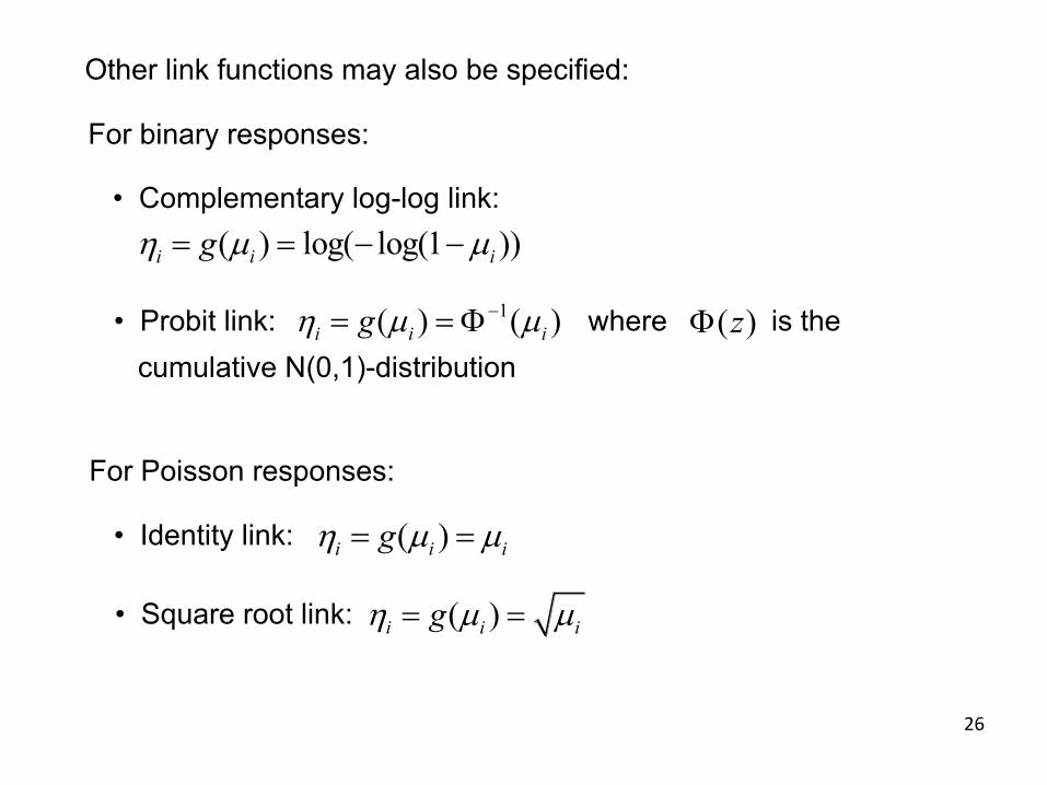
Other link functions may also be specified:

For binary responses:

• Complementary log-log link:( ) log( log(1 ))i i igh µ µ= = - -

• Probit link: where is the cumulative N(0,1)-distribution

1( ) ( )i i igh µ µ-= =F ( )zF

For Poisson responses:

• Identity link: ( )i i igh µ µ= =

• Square root link: ( )i i igh µ µ= =

27

Statistical inference in GLMs is performed as illustrated for logistic regression and Poisson regression

Estimation:

• Maximum likelihood (MLE)

Testing:

• Wald tests

• Deviance/likelihood ratio tests

28

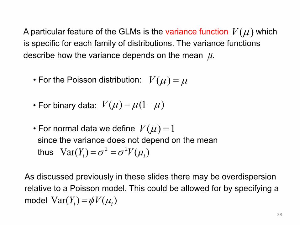
A particular feature of the GLMs is the variance function which is specific for each family of distributions. The variance functions describe how the variance depends on the mean .

• For the Poisson distribution:

( )V µ

µ

( )V µ µ=

( ) (1 )V µ µ µ= -

( ) 1V µ =

2 2Var( ) ( )s s µ= =i iY V

As discussed previously in these slides there may be overdispersionrelative to a Poisson model. This could be allowed for by specifying a model Var( ) ( )f µ=i iY V

• For binary data:

• For normal data we definesince the variance does not depend on the meanthus

Example: Number of sexual partnersStudy of sexual habits, Norwegian Institute of Public Health, 1988

29

no. sex-partners,

• Age, being single, having had HIV-test and was higher for men

However, the data was overdispersed. A “Pearson X2” statistic is

iY = 1,..., 8553i n= =A Poisson-regression found that the expected value increased with

22

1

ˆ( ) 51927ˆ

ni i

i i

YX µµ=

-= =å

which is large compared with residual degrees of freedom 8544.

2

1

ˆ( )1 51927ˆ 6.08ˆ 8544

ni i

i i

Yn p

µfµ=

-= = =

- åand should have been close to 1 if the Poisson model was correct.

An overdispersion term is estimated as

Standard errors and inference needs correction for overdispersion!

Correction for overdispersion

30

A overdispersed Poisson model is given by

•

•

0 1 1 2 2log( ) ....i i i p pix x xµ b b b b= + + + +

Var( ) fµ=i iY

This model can be fitted as a standard Poisson-regression, but the standard errors must be corrected to

* ˆse se f=where is the standard error from the Poisson-regression and the overdispersion is estimated as on the previous slide. Similarly the z-values become

sef̂

* ˆ/z z f=and p-values must be corrected correspondingly

Count data with over-dispersion – Quasi-likelihood

31

Although the corrections for overdispersion shown on the previous slide should be simple to carry out it is convenient that it is already implemented in R through a so-called

• Quasi-likelihood

The family-specification in the glm-command is given as “quasi” with arguments

• var=“mu”• link=log

glm(partners~Gender+Married+factor(HIVtest)+factor(agegr),family=quasi(link=log,var="mu"),data=part)

32

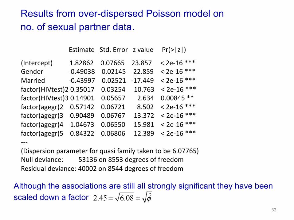
(Intercept) 1.82862 0.07665 23.857 < 2e-16 ***Gender -0.49038 0.02145 -22.859 < 2e-16 ***Married -0.43997 0.02521 -17.449 < 2e-16 ***factor(HIVtest)2 0.35017 0.03254 10.763 < 2e-16 ***factor(HIVtest)3 0.14901 0.05657 2.634 0.00845 **factor(agegr)2 0.57142 0.06721 8.502 < 2e-16 ***factor(agegr)3 0.90489 0.06767 13.372 < 2e-16 ***factor(agegr)4 1.04673 0.06550 15.981 < 2e-16 ***factor(agegr)5 0.84322 0.06806 12.389 < 2e-16 ***---(Dispersion parameter for quasi family taken to be 6.07765)Null deviance: 53136 on 8553 degrees of freedomResidual deviance: 40002 on 8544 degrees of freedom

Estimate Std. Error z value Pr(>|z|)

Results from over-dispersed Poisson model on no. of sexual partner data.

Although the associations are still all strongly significant they have been scaled down a factor ˆ2.45 6.08 f= =

33

Heteroscedastic linear model

Assume that the linear structure

0 1 1 2 2( ) ....i i i i p piE Y x x xµ b b b b= = + + + +

was found acceptable, but that the variance depended on as iµVar( ) fµ»i iY

One way to handle the non-constant variance could then be to specify a quasi-likelihood model with identity link and variance function “mu”

R can also handle variance structures and 3fµ2fµ

34

Generalized additive models (GAM)

We have encountered GAMs for• Multiple linear regression• Logistic regression

Any generalized linear model (GLM) can be extended to a GAM including Poisson regression models

A GAM consists of three parts• A family of distributions• A link function• An additive predictor

35

GAM, continued

Thus the first two components of a GAM are the same as for a GLM,but for the last component we replace the linear predictor

0 1 1 2 2 ....i i i p pix x xh b b b b= + + + +

with an additive predictor

0 1 1 2 2( ) ( ) .... ( )i i i p pif x f x f xh b= + + + +

where the linear terms are replaced by smooth functions j jixb ( )j jif x

Before fitting and plotting a GAM-model the library gam must be invoked (and installed).

Examples of use of GAM is found in Lecture 5, slide 19 and Lecture 7, slide 35.