sticky prices and volatile output

qWe thank an anonymous referee, Robert King and seminar participants at the Bank of England,CEPR/MMF workshop and the London Business School for comments.

*Corresponding author. Tel.: #44-171-706-6780; fax: #44-171-402-0718.E-mail address: [email protected] (A. Scott).

Journal of Monetary Economics 46 (2000) 621}632

Sticky prices and volatile outputq

Martin Ellison!, Andrew Scott",*!Department of Economics, European University Institute, Badia Fiesolana, Via dei Roccettini 9,

50016 S. Domenico di Fiesole (FI), Italy"Department of Economics, London Business School, Sussex Park, Regents Park, London NW1 4SA, UK

and CEPR

Received 12 February 1998; received in revised form 3 January 2000; accepted 3 February 2000

Abstract

We examine the e!ect of introducing a speci"c type of price stickiness into a stochasticgrowth model, subject to a cash in advance constraint. As in previous studies, we "nd theintroduction of price rigidities provides a substantial source of monetary non-neutralitywhich contributes signi"cantly to output volatility. We show that the introduction of thisform of sticky prices improves the model's performance at explaining in#ation butworsens it for output. The most dramatic failure of the model is the extremely high-frequency #uctuations in output that it generates. Sticky prices not only fail to producepersistent business cycle #uctuations but they generate extreme volatility at very highfrequencies. ( 2000 Elsevier Science B.V. All rights reserved.

JEL classixcation: E31; E32

Keywords: Business cycles; Cash in advance; Sticky prices

1. Introduction

A number of recent studies (e.g. Rotemberg and Woodford, 1992; King andWatson, 1996; King and Wolman, 1996; Yun, 1996) have introduced price

0304-3932/00/$ - see front matter ( 2000 Elsevier Science B.V. All rights reserved.PII: S 0 3 0 4 - 3 9 3 2 ( 0 0 ) 0 0 0 3 9 - 8

rigidities into a stochastic dynamic macroeconomic model. The motivation forthis work is clear: to try and explain the apparent impact that monetary shockshave on the business cycle (see, inter alia Sims, 1992; Christiano et al., 1995;Strongin, 1995) and the observed correlations between real and nominal vari-ables. While these studies have achieved some successes and suggested fruitfulareas for future research they have also revealed a potential problem with thesticky price assumption. As shown in Ball and Romer (1990) and Chari et al.(1996), sticky prices alone fail to account for the observed persistence of outputover the business cycle. The purpose of this paper is to reveal an additionalproblem with a particular class of sticky price models. Sticky price models failnot just because they do not generate enough output #uctuations at businesscycle frequencies but because they generate far too much volatility at very highfrequencies. The volatility induced at these high frequencies is far in excess ofthat observed in the data.

To establish our result, we use a standard monetary model (essentially that ofYun, 1996) which combines a stochastic growth model with a cash in advanceconstraint (Cooley and Hansen, 1995) and sticky prices (Calvo, 1983) solvedusing Parameterised Expectations (den Haan and Marcet, 1990) and show thatthis model:

(i) has the ability to o!er a better explanation of in#ation behaviour at allfrequencies;

(ii) generates short-run output #uctuations way in excess of that observed inthe data;

(iii) worsens the ability of the stochastic growth model to explain output#uctuations at business cycle frequencies.

While (i) and (iii) have been stressed in the literature (ii) has not beenemphasised to date.

The plan of the paper is as follows: In Section 2, we outline the modeleconomies we investigate while Section 3 discusses our calibration and solutionmethods. Section 4 then examines the performance of our simulated models inmatching the data while a "nal section concludes.

2. The model

We focus on a stochastic growth model consisting of a continuum of imper-fectly competitive "rms (distributed over the interval (0,1)) where consumers aresubject to a cash in advance constraint. We examine two assumptions about"rms: in our central case, "rms can change prices whenever they so desire andthe model is characterised by #exible prices; in the other case we follow Calvo(1983) and assume that in every period only a randomly selected group of "rmscan alter prices. This combination of stochastic growth model, cash in advance

622 M. Ellison, A. Scott / Journal of Monetary Economics 46 (2000) 621}632

1Ctactually represents a measure of total consumption and is de"ned by the aggregator function

(:10c(i)(e~1)@e di)e@(1~e) where e is the elasticity of demand.

constraint and sticky prices makes our model essentially a variant of Yun (1996).Readers wanting a more detailed economic explanation of the model shouldconsult Yun (1996) as in what follows we o!er only a mathematical outline.

Consumers are in"nitely lived and have preferences given by the utility function:

E0

=+t/0

btG[Cr

t(1!H

t)1~r]1~q

1!q H, (1)

where Ct

is consumption,1 Ht

the hours worked, b is the discount factor,u measures the weight of utility from consumption relative to utility from leisureand q is the coe$cient of relative risk aversion. Households are endowed withone unit of time each period and supply labour to "rms who produce intermedi-ate goods. Households are also engaged in accumulating capital which they rentto "rms. It is assumed that households enter period t with nominal moneybalances, m

t~1, carried over from the previous period. In addition, these bal-

ances are augmented with a lump sum transfer equal to (gt!1)M

t~1, where

Mt~1

is the aggregate money supply in period t!1 which, because of ourrepresentative agent model, equals m

t~1. The money stock then follows the law

of motion

Mt"g

tM

t~1, (2)

where we assume gtfollows the autoregressive process

ln(gt`1

)"ogln(g

t)#m

t`1, (3)

where mt`1

&iid(ln(g)(1!og),p2m ) and we assume g

tis revealed to all agents at

the beginning of period t. Household purchases are subject to the cash inadvance constraint:

PtC

t4m

t~1#(g

t!1)M

t~1, (4)

where Pt

is the aggregate price level (de"ned explicitly in (7) below) andassuming g

t'b,∀t is su$cient to ensure that this constraint always binds. The

capital stock obeys the law of motion kt"(1!d)k

t~1#x

twhere x

tdenotes

investment and d is the depreciation rate. The consumers' period by periodbudget constraint is

Ct#x

t#

mt!m

t~1P

t

4wtH

t#r

tK

t~1#Ph

t#(g

t!1)

Mt~1Pt

, (5)

where Phtrepresents the consumers share of pro"ts received from share holdings

and wtand r

tdenote the real wage and the rental price of capital, respectively.

M. Ellison, A. Scott / Journal of Monetary Economics 46 (2000) 621}632 623

2This is our main di!erence from the model of Yun (1996) who allows those who do not changeprices to their new optimal level to adjust prices by the rate of in#ation. As a result our modelcontains a greater degree of price rigidity.

The demand for intermediate good i is given by standard Dixit and Stiglitz(1977) preferences, namely

Dit"A

Pit

PtB

~eD

t, (6)

where Dtis the demand for the composite good at time t(:1

0D

t(i)(e~1)@edi)e@(e~1), e

is the elasticity of demand for good i and Ptis an aggregate of individual prices

de"ned by

Pt"AP

1

0

Pt(i)1~ediB

1@(1~e). (7)

The "rm produces output of good i, >itaccording to the production technology:

>it"h

tKi

a

t~1Hi

1~a

t!Fi, (8)

where Fitdenotes the "rm's "xed cost of production which we assume so as to

ensure long-run industry pro"ts are zero and where htis a stochastic productiv-

ity term following the process:

ln ht"oh ln h

t~1#c#e

t`1, (9)

where e&iid(0,p2e ). Firms are assumed to minimise costs which leads to "rst-order conditions:

wt"(1!a)mc

thtKa

t~1H~a

t,

rt"amc

thtKa~1

t~1H1~a

t,

(10)

where mctis the real marginal cost of production (MC

t/P

t) and period pro"ts

are de"ned as

Pit"A

Pit

Pt

!mctBA

Pit

PtB

~ehtKi

a

t~1Hi

1~a

t!Fi. (11)

In the case of #exible prices the "rm has to choose prices so as to maximise(11) subject to (6)}(10).

2.1. Inyexible prices

We assume, following Calvo (1983), that every period a proportion of "rms(1!u) are allowed to change their prices to a new optimal level while theremainder keep their prices "xed.2 The average duration of a price the "rm sets


is given by (1!u)/u. Denoting the new optimal price that "rms set by Pt,t

thisprice adjustment rule implies

P1~et

"(1!u)P1~et,t

#uP1~et~1

. (12)

A "rm will set its optimal price by maximising the present discounted value ofexpected future pro"ts with respect to P

t,twhere expected future pro"ts are

de"ned by

=+k/0

(ub)kEt

Kt`kK

tA

Pt,t

Pt`k

!mct`kBA

Pt,t

Pt`kB

~eht`k

Kia

t`k~1Hi

1~a

t`k, (13)

where Kt"E

t(bP

tjt`1

) and jt

denotes the consumer's marginal utility ofwealth. This de"nition of future pro"ts takes into account, both the stochasticnature of whether the "rm will change prices (u) and that the "rm will have tohold prices "xed during periods when it cannot change prices. Under in#exibleprices the "rm maximises (13) subject to (6)}(10). This leads to a "rst-ordercondition for P

t,tof

Pt,t"

e+=k/0

(ub)kEt[K

t`kPet`k

ht`k

Kia

t`k~1Hi

1~a

t`kmc

t`k]

(e!1)+=k/0

(ub)kEt[K

t`kPe~1t`k

ht`k

Kia

t`k~1Hi

1~a

t`k]. (14)

In the case of perfect price #exibility (u"0) this expression collapses to themore familiar P

t,t"eMC

t/(e!1).

3. Calibration and solution

We calibrate the model using UK quarterly data assuming a discount factorof 0.99 and a depreciation rate of 2.5%. Following the empirical analysis ofHolland and Scott (1998) we set a in the production function to 0.4436 andassume that the productivity shock follows the process

ln ht"0.0021#ln h

t~1#e

t, (15)

where pe"0.00925. Based on the panel data estimates of Attanasio and Weber(1993), we set the coe$cient of relative risk aversion equal to one so that utility islogarithmic. We set the weight of leisure with respect to consumption in theutility function such that the steady-state supply of labour is equal to 1

3. Using

the results of Garratt and Scott (1996), we used M0 (narrow money) to calibratethe money supply process such that

ln gt"0.011#0.3633 ln g

t~1#m

t, (16)

where pm"0.0122.


3The Hall et al. (1996) paper also reveals that only 20% of "rms change their prices once a quarterwhich suggests u"0.5 may overstate price #exibility. We therefore also performed simulations foru"0.25. These results are available upon request but the main "ndings of our paper remainunaltered.

Crucial to our simulation properties are the elasticity of demand and thedegree of price stickiness. Haskel et al. (1995) estimate the price to marginal costratio for the UK to be 1.94 which gives us a value of 2.64 for the elasticity ofdemand, e. A study of pricing policy in UK companies (Hall et al., 1996) "ndsthat approximately 6% of companies do not change their price over a year,suggesting u4"0.06 so that u+0.5 } only 50% of "rms are able to changetheir prices in a quarter.3

To solve the model we utilised the Parameterised Expectations Algorithm ofden Haan and Marcet (1990) which has the advantage of being able to capturenon-linearities present in the model which are normally excluded via the use ofquadratic approximations around the steady state. We used a second-orderpolynomial in the state variables (k

t~1,P

t~1,et, g

t) and included the cross-

products kt~1

etand P

t~1gtin order to arrive at an &accurate' solution. To gauge

accuracy we used the test statistic proposed by den Haan and Marcet (1994) andfor the #exible (in#exible) price model found 5.6% (4.2%) of simulations in thelower tail and 3.2% (6%) in the upper tail which we interpreted as stronggrounds for accuracy given the stringency of this test.

4. Results

Table 1 shows the stylised facts from UK data as well as from simulations ofour #exible and in#exible price (u"0.5) model. The data is for the UK over theperiod 1965}1995 and is explained in the Data Appendix. The relatively smallchanges in calibration that result from using US data do not alter the implica-tions of our analysis for sticky prices.

Both the #exible and in#exible price model do a reasonable job of reproduc-ing the observed volatility of prices and in#ation. The #exible price model,however, fails to reproduce the observed volatility of output and also fails toreplicate enough persistence. However, the problems with the sticky price modelare also apparent from Table 1 } it generates a huge increase in output volatilityin excess of that observed in the data and dramatically reduces the persistence ofoutput #uctuations. The explanation of these results can be seen in Fig. 1 whichshows estimated impulse-response functions of output with respect to a mone-tary shock. We estimate these impulse response functions using the methodo-logy of Blanchard and Quah (1989) and bivariate VARs and identify monetaryshocks by assuming they have no long-run impact on output. In the #exible


Table 1Stylised facts for output and in#ation

Cross-correlation of output with:Std.

Variable dev. t!3 t!2 t!1 t t#1 t#2 t#3

UK data

Output 1.66 0.434 0.624 0.810 1.000 0.810 0.624 0.434Prices 2.32 !0.439 !0.545 !0.605 !0.611 !0.524 !0.391 !0.216In#ation 1.03 !0.244 !0.240 !0.144 !0.019 0.171 0.266 0.360

Flexible price model

Output 1.12 0.267 0.462 0.700 1.000 0.700 0.462 0.267Prices 2.34 0.007 !0.035 !0.091 !0.177 !0.137 !0.108 !0.092In#ation 1.61 !0.030 !0.058 !0.078 !0.121 0.059 0.040 0.025

Inyexible price model

Output 3.72 !0.048 0.001 0.142 1.000 0.142 0.001 !0.048Prices 1.91 !0.302 !0.336 !0.300 0.359 0.357 0.300 0.238In#ation 1.33 !0.066 !0.042 0.062 0.925 0.004 !0.079 !0.084

Fig. 1. Impulse response function of monetary shocks on output.

price model the cash in advance constraint generates only a small non-neutralitysuch that the impulse response function rarely deviates from the horizontal axis.The sticky price model generates an impulse response function similar in shapeto that obtained from the data. However, the peak in the impulse response


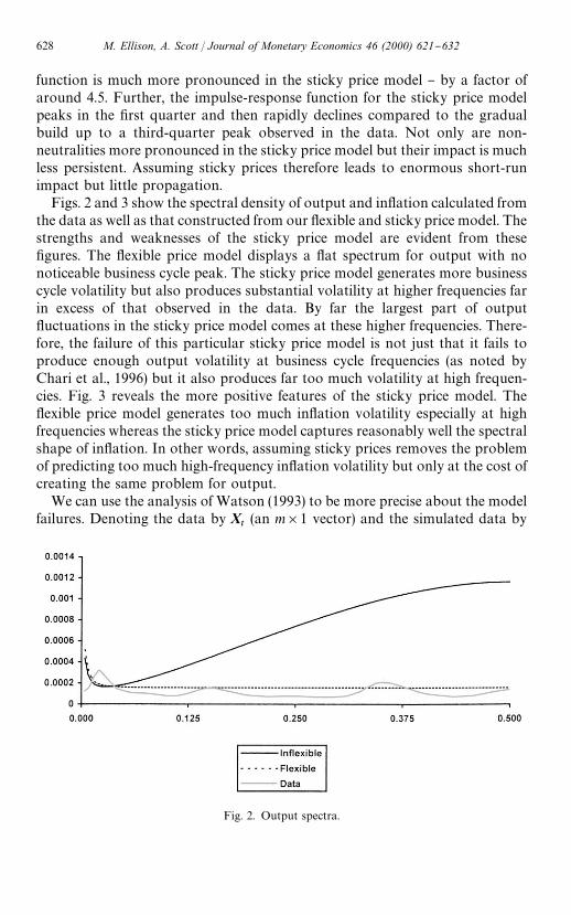
Fig. 2. Output spectra.

function is much more pronounced in the sticky price model } by a factor ofaround 4.5. Further, the impulse-response function for the sticky price modelpeaks in the "rst quarter and then rapidly declines compared to the gradualbuild up to a third-quarter peak observed in the data. Not only are non-neutralities more pronounced in the sticky price model but their impact is muchless persistent. Assuming sticky prices therefore leads to enormous short-runimpact but little propagation.

Figs. 2 and 3 show the spectral density of output and in#ation calculated fromthe data as well as that constructed from our #exible and sticky price model. Thestrengths and weaknesses of the sticky price model are evident from these"gures. The #exible price model displays a #at spectrum for output with nonoticeable business cycle peak. The sticky price model generates more businesscycle volatility but also produces substantial volatility at higher frequencies farin excess of that observed in the data. By far the largest part of output#uctuations in the sticky price model comes at these higher frequencies. There-fore, the failure of this particular sticky price model is not just that it fails toproduce enough output volatility at business cycle frequencies (as noted byChari et al., 1996) but it also produces far too much volatility at high frequen-cies. Fig. 3 reveals the more positive features of the sticky price model. The#exible price model generates too much in#ation volatility especially at highfrequencies whereas the sticky price model captures reasonably well the spectralshape of in#ation. In other words, assuming sticky prices removes the problemof predicting too much high-frequency in#ation volatility but only at the cost ofcreating the same problem for output.

We can use the analysis of Watson (1993) to be more precise about the modelfailures. Denoting the data by X

t(an m]1 vector) and the simulated data by


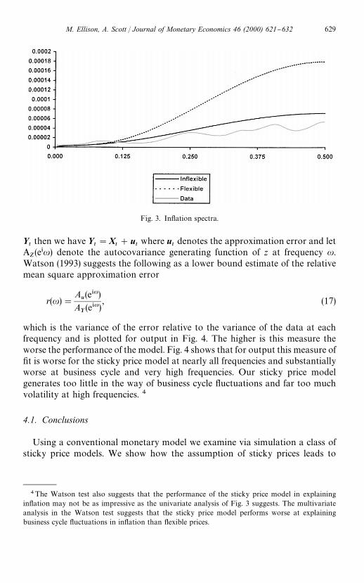
Fig. 3. In#ation spectra.

4The Watson test also suggests that the performance of the sticky price model in explainingin#ation may not be as impressive as the univariate analysis of Fig. 3 suggests. The multivariateanalysis in the Watson test suggests that the sticky price model performs worse at explainingbusiness cycle #uctuations in in#ation than #exible prices.

Ytthen we have Y

t"X

t#u

twhere u

tdenotes the approximation error and let

AZ(e*u) denote the autocovariance generating function of z at frequency u.

Watson (1993) suggests the following as a lower bound estimate of the relativemean square approximation error

r(u)"A

u(e*u)

AY(e*u)

, (17)

which is the variance of the error relative to the variance of the data at eachfrequency and is plotted for output in Fig. 4. The higher is this measure theworse the performance of the model. Fig. 4 shows that for output this measure of"t is worse for the sticky price model at nearly all frequencies and substantiallyworse at business cycle and very high frequencies. Our sticky price modelgenerates too little in the way of business cycle #uctuations and far too muchvolatility at high frequencies. 4

4.1. Conclusions

Using a conventional monetary model we examine via simulation a class ofsticky price models. We show how the assumption of sticky prices leads to


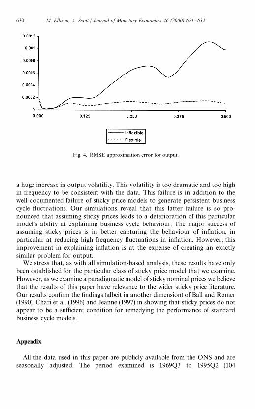
Fig. 4. RMSE approximation error for output.

a huge increase in output volatility. This volatility is too dramatic and too highin frequency to be consistent with the data. This failure is in addition to thewell-documented failure of sticky price models to generate persistent businesscycle #uctuations. Our simulations reveal that this latter failure is so pro-nounced that assuming sticky prices leads to a deterioration of this particularmodel's ability at explaining business cycle behaviour. The major success ofassuming sticky prices is in better capturing the behaviour of in#ation, inparticular at reducing high frequency #uctuations in in#ation. However, thisimprovement in explaining in#ation is at the expense of creating an exactlysimilar problem for output.

We stress that, as with all simulation-based analysis, these results have onlybeen established for the particular class of sticky price model that we examine.However, as we examine a paradigmatic model of sticky nominal prices we believethat the results of this paper have relevance to the wider sticky price literature.Our results con"rm the "ndings (albeit in another dimension) of Ball and Romer(1990), Chari et al. (1996) and Jeanne (1997) in showing that sticky prices do notappear to be a su$cient condition for remedying the performance of standardbusiness cycle models.

Appendix

All the data used in this paper are publicly available from the ONS and areseasonally adjusted. The period examined is 1969Q3 to 1995Q2 (104


observations), which we choose due to the unavailability of data on narrowmoney prior to 1969. Data and solution programs are available upon request. Thedata are:

(i) Real aggregate output is GDP at factor cost (C Million, 1990 prices); CSOcode CAOP.

(ii) Prices are measured using the GDP De#ator (1990"100); CSO codeDJCM.

(iii) In#ation is measured as the quarterly rate of change in the GDP de#ator.(iv) Narrow money M0 (C Million); CSO code AVAE.

References

Attanasio, O., Weber, G., 1993. Consumption growth, the interest rate and aggregation. Review ofEconomic Studies 60, 631}649.

Ball, L., Romer, D., 1990. Real rigidities and the non-neutrality of money. Review of Economic Studies57 (2), 183}203.

Blanchard, O., Quah, D., 1989. The dynamic e!ects of aggregate demand and supply disturbances.American Economic Review 79, 655}673.

Calvo, G.A., 1983. Staggered prices in a utility-maximising framework. Journal of Monetary Econ-omics 12, 383}398.

Chari, V., Kehoe, P., McGrattan, E., 1996. Sticky price models of the business cycle: can the contractmultiplier solve the persistence problem? Federal Reserve Bank of Minneapolis Research Depart-ment Sta! Report No. 217.

Christiano, L., Eichenbaum, M., Evans, C., 1995. The e!ects of monetary policy shocks: some evidencefrom the #ow of funds. Review of Economics and Statistics 78, 16}34.

Cooley, T., Hansen, G.D., 1995. Money and the business cycle. In: Cooley, T.F. (Ed.), Frontiers ofBusiness Cycle Research. Princeton University Press, Princeton, NJ, pp. 1}38.

Dixit, A., Stiglitz, J., 1977. Monopolistic competition and optimum product diversity. AmericanEconomic Review 67, 297}308.

den Haan, W., Marcet, A., 1990. Solving the stochastic growth model by parameterising expectations.Journal of Business and Economic Statistics 8, 31}34.

den Haan, W., Marcet, A., 1994. Accuracy in simulations. Review of Economic Studies 61, 3}17.Garratt, A., Scott, A., 1996. Money and Output: A Reliable Predictor or Intermittent Signal?

Cambridge University, Cambridge, Mimeo.Hall, S., Walsh, M., Yates, T., 1996. How do UK companies set prices?. Bank of England Quarterly

Bulletin 36, 2.Haskel, J., Martin, C., Small, I., 1995. Price, marginal cost and the business cycle. Oxford Bulletin of

Economics and Statistics 57, 25}41.Holland, A., Scott, A., 1998. The determinants of UK business cycles. Economic Journal 108,

1067}1092.Jeanne, O., 1997. Generating real persistent e!ects of monetary shocks: how much nominal rigidity

do we really need? NBER working paper no. 6258.King, R., Watson, M., 1996. Money, prices, interest rates and the business cycle. Review of Economics

and Statistics 78 (1), 35}53.King, R., Wolman, A., 1996. In#ation targeting in a St. Louis model of the 21st century. Federal

Reserve Board of St. Louis Review 78 (3), 83}107.


Rotemberg, J., Woodford, M., 1992. Oligopolistic pricing and the e!ects of aggregate demand oneconomic activity. Journal of Political Economy 100, 1153}1207.

Sims, C.A., 1992. Interpreting the macroeconomic time series facts: the e!ects of monetary policy.European Economic Review 36, 975}1011.

Strongin, S., 1995. The identi"cation of monetary policy disturbances: explaining the liquidity puzzle.Journal of Monetary Economics 35, 463}497.

Watson, M., 1993. Measures of "t for calibrated models. Journal of Political Economy 101, 1011}1041.Yun, T., 1996. Nominal price rigidity, money supply endogeneity and business cycles. Journal of

Monetary Economics 37, 345}370.


sticky prices and volatile output

Documents