STICKY-PRICE MONETARY MODEL OF EXCHANGE RATE: A COINTEGRATION ANALYSIS

A. Tarkan Çavuşoğlu Middle East Technical University and Mersin University

Department of Economics, 06531, Ankara, Turkey E-mail: b060404@orca.cc.metu.edu.tr

ABSTRACT

This study attempts to investigate empirically the presence of any identifiable and plausible long-run relationships among the variables of a system which is expected to reflect the exchange rate (TL/$) dynamics in Turkey. In this context, “the sticky-price monetary model of exchange rate” developed by Dornbusch (1976) is utilized. The study is limited to long-run analysis based on the maximium likelihood approach by Johansen (1988). The cointegration analyses with quarterly data for the period 1984:1-1996:3 result in three long-run relationships explaining inflation, uncovered interest parity condition and depreciation of nominal exchange rate. Inflation seems to be stationary around minor influences from aggregate demand and real reserve money balances, while depreciation of the nominal exchange is explained through inflation, nominal interest rate and velocity of money in circulation. Inflation appears to be the most influential factor on the depreciation of the domestic currency and has no feedback from the nominal depreciation. Key Words: Cointegration, identification, exchange rate, Turkey. JEL Classification: C32, F43 Acknowledgement: I am grateful to Dr.Erdal Özmen for his guidance and helpful comments for the improvement of this paper.

1

I. INTRODUCTION

The collapse of the Bretton Wood system of fixed exchange rates in March 1973 gave way to

the development of monetary models of exchange rate determination. Monetary approach has become

quite popular and is widely used in forecasting the nominal exchange rate in an open economy

operating under a floating exchange rate system. In this regard, recent studies testing the forecasting

performance of the monetary models have found evidence supporting the presence of long-run

equilibrium relationships between the exchange rate and its fundamentals.

Turkey experienced a fixed exchange rate system until the introduction of market-oriented

structural policies in 1980. The external financial liberalization process has accelerated significantly

since 1984 when most of the barriers for international trade were abolished. The domestic banks were

allowed to accept foreign currency deposits, and in this way a formal foreign exchange market was

allowed to be institutionalized. However, in the market, the exchange rate was not floating freely until

the end of June 1985, because the commercial banks were required to determine their rates within a 6

% band around the Central Bank’s official foreign exchange rate, rather than to determine them freely

(Altınkemer and Ekinci, 1992: 89-97).

This study attempts to investigate empirically the presence of any identifiable long-run

relationships among the variables of a system that is expected to reflect the exchange rate dynamics

for the 1984:1- 1996:3 periods in Turkey with quarterly data. As mentioned above, the year 1984 is

assumed to be the beginning of the major attempts to liberalize international trade, the exchange and

payment system. The analysis is based on the sticky-price monetary model of exchange rate

introduced by Dornbusch (1976).

The study is limited to the long-run analysis that is performed by employing the maximum

likelihood approach proposed by Johansen (1988). Throughout the study, the empirical analyses

exploit several issues of the theory of cointegration.

2

II. THE THEORETICAL MODEL

The monetary exchange rate determination models formulated under the assumption of the

validity of the Purchasing Power Parity (PPP) condition may not reflect the dynamics of a small

inflationary economy. Dornbusch (1976), retaining the long-run PPP hypothesis, developed a model

in which the relevant balance of payments equilibrium condition is reflected by the Uncovered Interest

Parity (UIP) and the domestic price level is a slowly-adjusting variable. The basic equations of the

simplified version of this model1 are

yt = a1 (∆et - ∆pt) - a2 rt (1)

(m-p)t = b1 yt - b2 Rt - b3 ∆pt (2)

rt = Rt - ∆pt (3)

Rt = Rt* + ∆et (4)

yt = y t (5)

All variables, except for Rt, are in natural logarithms. yt , (m-p)t , rt , Rt , ∆pt , ∆et and Rt* denote,

respectively, the real income which is proxied by the industrial production index, the real reserve

money stock, the real interest rate, the nominal interest rate proxied by the three-month time deposit

rate, the rate of inflation in the wholesale price index, the change in the nominal exchange rate

(Turkish Lira/ US Dollar) and the foreign nominal interest rate proxied by the three-month commercial

paper rate2.

Note that, in equation (1), which denotes the goods market equilibrium, (∆et - ∆pt) is the

change in the log of EP/P* where ∆pt* is normalized to unity. Furthermore, utilizing (∆et -∆pt) rather

than (et - pt) in equation (1) and formulating the money market equilibrium as in equation (2) by

using (m-p)t and including ∆pt, are all done for eliminating the I(2) components3 (this will be clarified

in the following part of the study). The equations (3), (4) and (5) show respectively the real interest

rate, the UIP hypothesis and the long-run equilibrium condition of the real domestic output.

1 See McCallum (1996), Isard (1995) and MacDonald (1988) for the details of the model. 2 Industrial production index (yt) data (quartely averages) are taken from the State Institute of Statistics data base. Data on nominal exchange rate (et), wholesale price index (pt) and three-month time deposit rates (Rt) are taken from the data base of the Central Bank of the Republic of Turkey. Reserve money (mt) and US three-month commercial paper rates (Rt*) are from the International Financial Statistics, CD-ROM. 3 See Johansen (1992) and Hendry and Mizon (1993) for the utilization of this form of money market equilibrium condition.

3

III. EMPIRICAL RESULTS

Integration characteristics of the series

Our first step in the cointegration analysis is to investigate the individual characteristics of the

series used in the model by utilizing the augmented Dickey-Fuller (1981) test, for a sample period

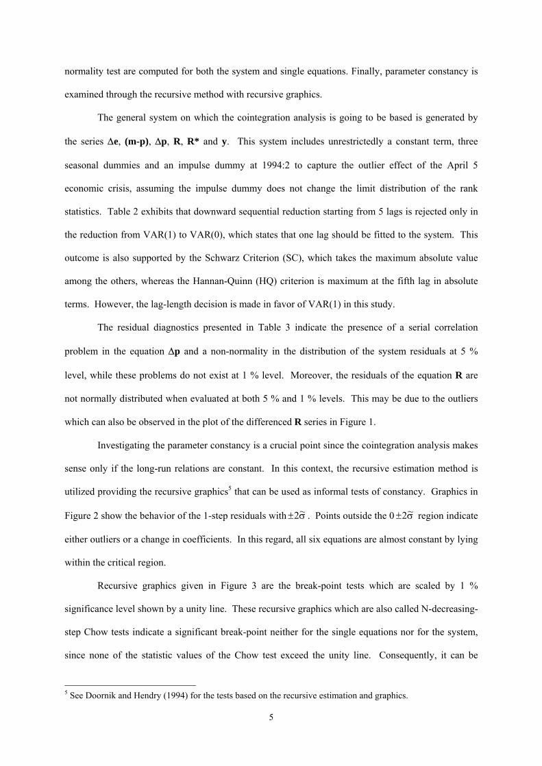
1984:1-1996:3. The plots of the series in levels and differences, exhibited in Figure 1, may give some

idea about the stationarity and non-stationarity of these series. The plots of the differenced nominal

exchange rate and price index series seem to indicate that these series are generated by the I(2)

process, while the others seem to be generated by the I(1) process. Moreover, the plots clearly show

the outlier effect of the economic crisis of April 5, 1994 in Turkey. However, the formal conclusion

about the integration properties of the series can be arrived at using the unit root tests (see Table 1).

All series, except for the price index p and e, appear to be generated by the I(1) process at the

5% significance level. In the cointegration analysis, which is going to be carried out next, the series

∆e and ∆p are treated as I(1) series. In this regard, equations (1) and (2) given in part II are modified

with respect to this outcome. Therefore, the real exchange rate expression (e-p) rather appears to be

indicated by a change in the real exchange rate (∆e-∆p) in equation (1) and moreover, the money

market equilibrium condition, mt - pt = b1yt - b2Rt , is modified as it appears in equation (2), so that it is

possible to observe the real reserve money stock effects.

The system tests of congruency

The essential step to develop a structural model of a system is to achieve a congruent

representation of the data. In this regard, congruency requires a correctly specified lag-structure for

the system of which the residuals are well-behaved and the parameter constancy is satisfied. In

determining the lag-structure of the VAR(s) system, two information criteria, those of Schwarz and

Hannan-Quinn, and a sequential reduction procedure4 are utilized. For the residual analysis, an F-

version of the LM test for autocorrelation and ARCH, White test for heteroskedasticity and a

4 See Doornik and Hendry (1994) for the computation of the sequential reduction testing procedure.

4

normality test are computed for both the system and single equations. Finally, parameter constancy is

examined through the recursive method with recursive graphics.

The general system on which the cointegration analysis is going to be based is generated by

the series ∆e, (m-p), ∆p, R, R* and y. This system includes unrestrictedly a constant term, three

seasonal dummies and an impulse dummy at 1994:2 to capture the outlier effect of the April 5

economic crisis, assuming the impulse dummy does not change the limit distribution of the rank

statistics. Table 2 exhibits that downward sequential reduction starting from 5 lags is rejected only in

the reduction from VAR(1) to VAR(0), which states that one lag should be fitted to the system. This

outcome is also supported by the Schwarz Criterion (SC), which takes the maximum absolute value

among the others, whereas the Hannan-Quinn (HQ) criterion is maximum at the fifth lag in absolute

terms. However, the lag-length decision is made in favor of VAR(1) in this study.

The residual diagnostics presented in Table 3 indicate the presence of a serial correlation

problem in the equation ∆p and a non-normality in the distribution of the system residuals at 5 %

level, while these problems do not exist at 1 % level. Moreover, the residuals of the equation R are

not normally distributed when evaluated at both 5 % and 1 % levels. This may be due to the outliers

which can also be observed in the plot of the differenced R series in Figure 1.

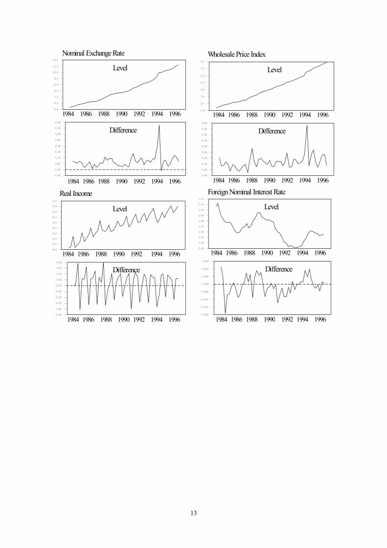
Investigating the parameter constancy is a crucial point since the cointegration analysis makes

sense only if the long-run relations are constant. In this context, the recursive estimation method is

utilized providing the recursive graphics5 that can be used as informal tests of constancy. Graphics in

Figure 2 show the behavior of the 1-step residuals with ±2~σ . Points outside the 0 ±2~σ region indicate

either outliers or a change in coefficients. In this regard, all six equations are almost constant by lying

within the critical region.

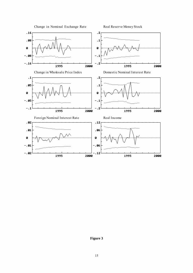
Recursive graphics given in Figure 3 are the break-point tests which are scaled by 1 %

significance level shown by a unity line. These recursive graphics which are also called N-decreasing-

step Chow tests indicate a significant break-point neither for the single equations nor for the system,

since none of the statistic values of the Chow test exceed the unity line. Consequently, it can be

5 See Doornik and Hendry (1994) for the tests based on the recursive estimation and graphics.

5

concluded that 1-lag VAR representation is data congruent and indicates no evidence of mis-

specification against constructing a structural model of the system.

Cointegration Analysis

The cointegration analysis is based on a maximum likelihood approach proposed by Johansen

(1988, 1991 and 1995) and Johansen and Juselius (1990). The system utilized for cointegration can be

represented by a vector error correction mechanism (VECM) for the long-run endogenous variables:

, t =1,....,T (6) ∆ Π Γ ∆ ΦZ Z Z Dt t ii

s

t t= + + + + +−=

−

−∑11

1

1 µ ψ ε I 94 t

n

Π= +1

where is, now, a 6×1 vector of the endogenous variables ∆e, (m-p), ∆p, R, R*

and y. , µ is a constant term, D

Z z zt = ′( , ,..., )1 2 z

= is

iΠ Π Γ− = −=∑ ∑I

i jj i

s

1, t are three seasonal dummies, I94 is

an impulse dummy and εt is an independent identically distributed error term. Π6×6 is the long-run

coefficient matrix, which can be decomposed into r distinct cointegrating vectors of and an

adjustment (feedback or loading) matrix

′×β r 6

α 6× r (Π = ′αβ ). In this respect, testing for cointegration is

investigating the number of r linearly independent columns in Π. The elements of α indicate the speed

of adjustment of a particular variable when there is a disturbance in the equilibrium relation, while the

elements of β indicate the long-run responses of the variables in the equilibrium relationship.

Part (1) of Table 4 exhibits the cointegration test results of the VAR(1) system. These results

indicate the presence of r=3 cointegrating vectors in the system since the maximal eigenvalue (λ-max)

and trace eigenvalue (λ-trace) statistics reject the null hypothesis of r=2, but do not reject the null that

there are at most three cointegrating vectors, r ≤ 3.

In the second part of Table 4, these three cointegrating vectors and their adjustment

coefficients are computed by standardizing the first one with respect to ∆p, and the other two with

respect to ∆e. The individual long-run exclusion test statistics which are computed and given in

parentheses under each β-coefficient are utilized as an informal test statistic6 in order to test whether

6 See Juselius and Hargreaves (1992) for the usage of this test statistic.

6

or not the variables have any explanatory power in each of the cointegrating vectors. Later, this test

statistic is going to be used for imposing exclusion restrictions in identifying the cointegration vectors.

On the other hand, individual test statistics for weak-exogeneity (or speed of adjustment) given in

parentheses under each α-coefficient, tests whether or not there is an adjustment towards the stationary

state when there are short-run deviations from the long-run path of a given series. In this respect, at

first glance, standardizing the third eigen-vector with respect to ∆e (see the second part of Table 4),

which does not adjust to a shock since its adjustment coefficient is positive and insignificant, seems to

be inconsistent theoretically. However, a negative and significant adjustment coefficient can be

achieved when an economic structure is imposed through the identification restrictions. Therefore, the

interpretation of these coefficients is left to the next part of the study.

The third part of Table 4 exhibits that all of the six variables are statistically significant in the

cointegration space, owing to the rejection of the long-run exclusion hypothesis and, therefore, they all

contribute to the determination of the long-run equilibrium solution. Moreover, all of the variables

entering the cointegration space are non-stationary with respect to the rejection of the stationarity

hypothesis, as expected. Finally, according to the weak-exogeneity test statistics7 given in the third

part of Table 4, the weak-exogeneity status of (m-p) and R* are not rejected, which is a consistent

outcome with the economic model presented in part II. Thus, ∆e, ∆p, R and y are determined within

the system, while (m-p) and R* are weakly-exogenous for the parameters of the system.

Identifying the long-run structure of the system

Developing a parsimonious model from a data-congruent statistical system involves imposing

a structure on it by exploiting economic theory8. In this regard, in Doornik and Hendry’s (1994: 172)

words, “a test of over-identifying restrictions is equivalent to a test of whether the restricted reduced

form parsimoniously encompasses the unrestricted reduced form”. Moreover, since conditioning a

model on the weakly exogenous variables may improve its statistical specification, it is better to

impose the over-identification restrictions on the conditional model.

7 See Engle et al. (1983) and Johansen (1992) for the weak-exogeneity concept.

7

Depending on the weak-exogeneity results reported in table 4, the model is conditioned on the

series (m-p) and R*. The exclusion restrictions imposed on each of the three cointegrating vectors are

based on the individual exclusion test statistics attached to the β-coefficients computed in the second

part of Table 4. According to these statistics, in the first cointegration vector, ∆e, R and R* have no

statistical significance. In the second one, (m-p), R and y, and in the third one, only R* should be

excluded from the vectors. As for further restrictions, to impose the UIP structure on the second

cointegrating vector, the coefficients of ∆e and R* are restricted to be equal and to have a sign

opposite to the coefficient of ∆p. In the third vector, the coefficients of (m-p) and y are restricted to

denote the velocity of circulation of money9. Consequently, the relevant restricted β matrix and

design matrices will be as follows:

0 1 1 0 0 0 1 1 0 0 0 * 0 c 1 0 0 0 0 0 1 0

β= 1 -1 * H1= 0 1 0 H2= -1 H3= 0 1 0 0 0 0 * 0 0 0 0 0 0 0 1 0 1 0 0 0 0 1 0 0 0 0 * 0 -c 0 0 1 0 0 0 -1 0

The corresponding likelihood ratio test of over-identifying restrictions is χ2(4) = 7.36 (0.12). Since,

according to this statistic, the over-identifying restrictions imposed on the conditional model are not

rejected, the model constitutes a valid reduction of the system and allows for plausible economic

interpretations. According to the identified vectors given in Table 5, the first vector indicates that

inflation is stationary, but influenced by the aggregate demand and real reserve money balances, even

though these influences are minor in magnitude. The second vector represents an equation that

explains the rate of depreciation (or its expectation) through the difference between the domestic rate

of inflation and foreign nominal interest rate. Such a long-run relationship may be considered as the

indication of the uncovered interest parity condition when the domestic nominal interest rate is

expected to converge to the domestic rate of inflation in the long-run through the Fisher equation, i.e.

(R-∆p) ∼ I(0) and hence, ∆p=R*+∆e. The third vector is considered to be a long-run relationship

8 See Johansen and Juselius (1994) for the application of the identification of a long-run structure. 9 See Hendy and Doornik (1994) and Hendry (1995) for the usage of inverse velocity (m-p-y).

8

explaining the nominal depreciation of the domestic currency by the domestic rate of inflation ∆p, the

nominal interest rate R and the (inverse) velocity (m-p)-y. The negative coefficient of R in this vector

may reflect the appreciation of the domestic currency when financial capital inflows are maintained

through higher nominal interest rates. The negative coefficient of inverse velocity (m-p-y) indicates

that there is a direct relationship between velocity and exchange rates. On the determination of the

nominal exchange rate inflation appears to be more influential than the effects of the nominal interest

rate and velocity.

Note that each of these three long-run relationships identified through an economic structure

adjusts to short-run deviations from the long-run equilibrium, indicating the long-run stability of the

variables. Moreover, the adjustment coefficients of the third vector indicate that there is a strong feed-

back between ∆e and R, so that depreciation has a significant role in restoring the equilibrium in the

money market through its effects on the nominal interest rates, whereas the adjustment coefficient of

∆p indicates that inflation is an exogenous factor in determining the rate of depreciation, inconsistent

with some claims that depreciation feeds inflation.

IV. CONCLUSION

The data-congruent statistical system generated by the variables of the sticky-price monetary

model provides a parsimonious model which consists of plausible long-run economic relationships for

the small inflationary Turkish economy. The unrestricted cointegration estimation provides weak-

exogeneity test results which are consistent with the theoretical model presented in the second part of

the study. Next, conditioning the model on these weakly exogenous variables and imposing an

economic structure through over-identification restrictions are not rejected and provide three long-run

relations to be explained. The first relation indicates that the rate of inflation is stationary through

minor influences from the aggregate demand and real reserve money balances. The second one shows

that the uncovered interest parity condition holds. The last restricted vector explains the change in the

nominal exchange rate through price inflation, nominal interest rates and velocity of money. The rate

of inflation appears to be more influential on the nominal depreciation of the domestic currency than

9

the direct effects from the money market, and has no feedback from the rate of depreciation.

Moreover, there seems to be a feedback relationship between the rate of depreciation and nominal

interest rate.

Table 1 Unit Root Test Statistics

Levels 1st Differences 2nd Differences ADF(s) ADF(s) ADF(S)

series no trend trend no trend no trend e 1.91 (4) -0.96 (4) -2.73 (4) -7.32**(1)

(m-p) -2.82 (1) -2.63 (1) -9.68**(0) - p 2.99 (0) -1.38 (0) -2.10 (2) -9.56**(1) R -0.88 (2) -4.63**(0) -7.31**(1) -

10

R* -1.99 (5) -2.95 (5) -3.47* (0) - y -1.21 (3) -3.37 (0) -4.88**(2) -

All the test regressions contain three seasonal dummies and, except for the 2nd differenced series, all regressions contain a constant term. Figures in parentheses denote augmentation lag-length of the ADF regression. (*) and (**) denote the rejection of the null hypothesis at the 5 % and 1 % significance levels respectively, where the critical values are from MacKinnon (1991).

Table 2 Choice of the lag-length of the system

VAR(s) VAR(5) VAR(4) VAR(3) VAR(2) VAR(1) VAR(0) VAR(5)

- - - - - -

VAR(4)

0.8462 F(36,22)

- - - - -

VAR(3)

0.9476 F(72,33)

1.1286 F(36,51)

- - - -

VAR(2)

0.9998 F(108,35)

1.1494 F(72,65)

1.1393 F(36,77)

- - -

VAR(1)

1.0357 F(144,37)

1.1701 F(108,70)

1.1524 F(72,98)

1.1393 F(36,103)

- -

VAR(0)

4.1805** F(180,37)

5.3921** F(144,72)

6.6655** F(108,104)

9.5368** F(72,130)

21.440** F(36,130)

-

SC -36.60 -36.12 -36.59 -37.77 -39.35 -33.90 HQ -41.89 -40.50 -40.07 -40.34 -41.01 -34.65

(**) denotes the rejection of reduction from VAR(s) to VAR(s-i) at 1 % level. Bold values of SC and HQ indicate the column of the appropriate VAR(s) to be chosen.

Table 3

Single equation and system residual diagnostics equations AR (1-4)

F(4, 30) Normality χ2(2)

Heterosk. F(12, 21)

ARCH F(4, 26)

∆e 0.5722 2.1741 0.1864 0.8337 (m-p) 0.6055 0.0541 1.1627 0.8723 ∆p 3.3725* 3.7881 0.9981 0.4109 R 0.7111 12.406** 0.3866 0.1384

R* 1.2113 0.0850 0.5159 1.0311 y 0.6431 2.4259 0.8361 0.3810

system AR(1-4) F(144, 37)

Normality χ2(12)

Heterosk. F(252, 42)

-

VAR(1) 1.3292 21.922* 0.3044 - (*) and (**) denote the rejection at 5 % and 1 % levels respectively.

Table 4 Cointegration Analysis

(1) Cointegration test statistics

Ho: r = 0 r ≤ 1 r ≤ 2 r ≤ 3 r ≤ 4 r ≤ 3 eigen-values 0.8397 0.5648 0.4621 0.2319 0.0743 0.0002

λ-max 89.71* 40.76* 30.38* 12.93 3.78 0.01 λ-max (%90) 24.63 20.90 17.15 13.39 10.60 2.71

λ-trace 177.6* 87.86* 47.10* 16.72 3.79 0.01

11

λ-trace (%90) 89.37 64.74 43.84 26.70 13.31 2.71 (2) Standardized eigen-vectors βi and adjustment coefficients αI

Variables β1 β2 β3 α1 α2 α3

∆e 0.404 (2.85)

1.000 (8.37)*

1.000 (16.96)*

-0.914 (-14.017)*

-0.376 (-2.990)*

0.044 (0.685)

(m-p) 0.266 (4.17)*

0.081 (0.18)

-1.218 (14.22)*

0.068 (0.906)

-0.050 (-0.343)

0.192 (2.567)*

∆p 1.000 (7.62)*

-1.535 (10.27)*

0.317 (16.32)*

-0.499 (-11.274)*

0.326 (3.821)*

-0.098 (-2.235)

R 0.099 (1.06)

0.050 (0.12)

-0.859 (11.69)*

-0.749 (-7.928)*

0.171 (0.940)

0.299 (3.177)*

R* -0.514 1.260 1.672 0.013 -0.018 -0.014

y (0.98) -0.333 (9.62)*

(4.66)* 0.057 (0.15)

(3.35) 0.970

(17.35)*

(1.567) 0.042

(0.791)

(-1.146) 0.293

(2.864)*

(-1.745) -0.130

(-2.456)* (3) Tests for long-run exclusion (LE), stationarity (S) and weak-exogeneity (WE)

χ2(3) ∆e (m -p) ∆p R R* y LE 28.18* 18.57* 34.21* 12.87* 8.99* 27.12* S 11.13* 20.03* 14.86* 27.67* 26.74* 29.00*

WE 68.86* 5.75 56.81* 39.16* 5.13 11.53* Figures in parentheses under βi’s are likelihood ratio test statistics with χ2 (1) distribution and the ones under αi’s are t-statistics which test the statistical insignificance of the coefficients at 5 % level. The rejection of the hypothesis of insignificance is denoted by (*).

Table 5 Over-identification analysis

Variables β1 β2 β3 α1 α2 α3

∆e 0.000 1.000

1.000

-1.123 (-9.117)*

-0.278 (-1.386)

-0.323 (-3.453)*

(m-p)

0.059

0.000 0.751

- - -

∆p 1.000

-1.000

-1.646

-0.881 (11.727)*

0.126 (1.035)

-0.043 (-0.755)

R 0.000

0.000 0.699

-0.949 (-5.701)*

0.961 (3.552)*

-0.681 (-5.381)*

R*

0.000 1.000

0.000 - - -

y -0.105

0.000 -0.751

-0.125 (-1.278)

-0.106 (-0.668)

0.229 (3.076)*

(*) denotes the rejection at 5 % significance level for both χ2(1) and t statistics of the individual exclusion and weak-exogeneity testing procedures respectively.

Figure 1 Plots of the series in levels and differences

12

Nominal Exchange Rate

Level

1984 1986 1988 1990 1992 1994 19965.6

6.4

7.2

8.0

8.8

9.6

10.4

11.2

12.0

Difference

1984 1986 1988 1990 1992 1994 1996-0.08

0.00

0.08

0.16

0.24

0.32

0.40

0.48

0.56

0.64

Wholesale Price Index

Level

1984 1986 1988 1990 1992 1994 19961.8

2.7

3.6

4.5

5.4

6.3

7.2

8.1

Difference

1984 1986 1988 1990 1992 1994 19960.00

0.05

0.10

0.15

0.20

0.25

0.30

0.35

0.40

0.45

Real Income

Level

1984 1986 1988 1990 1992 1994 19964.1

4.2

4.3

4.4

4.5

4.6

4.7

4.8

4.9

5.0

Difference

1984 1986 1988 1990 1992 1994 1996-0.25

-0.20

-0.15

-0.10

-0.05

-0.00

0.05

0.10

0.15

0.20

Foreign Nominal Interest Rate

Level

1984 1986 1988 1990 1992 1994 19961.03

1.04

1.05

1.06

1.07

1.08

1.09

1.10

1.11

1.12

Difference

1984 1986 1988 1990 1992 1994 1996-0.020

-0.015

-0.010

-0.005

0.000

0.005

0.010

0.015

13

Real Reserve Money Stock

Level

1984 1986 1988 1990 1992 1994 199625.9

26.0

26.1

26.2

26.3

26.4

Difference

1984 1986 1988 1990 1992 1994 1996-0.15

-0.10

-0.05

0.00

0.05

0.10

0.15

Nominal Interest Rate

Level

1984 1986 1988 1990 1992 1994 19961.28

1.44

1.60

1.76

1.92

2.08

2.24

2.40

Difference

1984 1986 1988 1990 1992 1994 1996-0.6

-0.4

-0.2

-0.0

0.2

0.4

0.6

Figure 2 Recursive graphics of 1-step residuals ±2~σ

14

C h a n g e i n N o m i n a l E x c h a n g e R a t e R e a l R e s e r v e M o n e y S t o c k

C h a n g e i n W h o le s a l e P r i c e I n d e x D o m e s t i c N o m i n a l I n t e r e s t R a t e

F o r e i g n N o m i n a l I n t e r e s t R a t e R e a l I n c o m e

Figure 3

15

N↓ step Chow test for the equations and system

R e a l R e s e r v e M o n e y S t o c k

C h a n g e i n W h o l e s a l e P r i c e I n d e x

C h a n g e i n N o m i n a l E x c h a n g e R a t e D o m e s t i c N o m i n a l I n t e r e s t R a t e

F o r e i g n N o m i n a l I n t e r e s t R a t e

R e a l I n c o m e

S y s t e m C h o w T e s t

REFERENCES

Altınkemer, M. and N. Ekinci (1992) Capital account liberalization: The case of Turkey,

16

NewPerspectives on Turkey, 8, 89-108.

Dickey,

Dornbu f Political Economy, 84,

1161-76.

le R. F., Hendry, D. F. and Richard J. F. (1983) Exogeneity, Econometrica, 51, 277-304.

Hendry, D. F. (1995) Dynamic Econometrics, New York: Oxford University Press Inc.

Hendry, D. F. and G. E. Mizon (1993) Evaluating dynamic econometric models by encompassing the

VAR, In Phillips, P. C. B. (ed.), Models, methods and applications of econometrics, pp. 272-

300, Oxford: Basil Blackwell.

Isard, P. (1995) Exchange rate economics, Cambridge University Press.

Johansen, S. (1988) Statistical Analysis of Cointegration Vectors, Journal of Economic

Dynamics and Control, 12, 231-54.

Johansen, S. (1991) Estimation and hypothesis testing of cointegration: vectors in Gaussian vector

autoregressive models, Econometrica, 59(6), 1551-80.

Johansen, S. (1992) Testing weak exogeneity and the order of cointegration in UK money demand

data, Journal of Policy Modelling, 14(3), 313-34.

Johansen, S. (1995) Likelihood-Based Inference in Cointegrated Vector Auto-Regressive Models,

Oxford University Press Inc.

Johansen, S. and K. Juselius (1990) Maximum likelihood estimation and inference on cointegration-

with applications to the demand for money, Oxford Bulletin of Economics and Statistics,

52(2), 169-210.

Johansen, S. and K. Juselius (1994) Identification of the long-run and the short-run structure: An

application to the ISLM model, Journal of Econometrics, 63, 7-36.

D.A. and W. A. Fuller (1981) Likelihood ratio statistics for autoregressive time series with a

unit root, Econometrica, 49, 1057-72.

Doornik, J.A. and D.F. Hendry (1994) PcFiml 8.0 Interactive econometric modelling of dynamic

systems, London: International Thomson Publishing.

sch, R. (1976) Expectations and exchange rate dynamics, Journal o

Eng

17

18

Juselius, K. and C. P. Hargreaves (1992) Long-run relations in Australian monetary data, in

Hargreaves, G. P. (ed.) Macroeconomic modelling of the long-run, Aldershot: Edward Elgar.

MacCallum, B. T. (1996) International Monetary Economics, Oxford University Press.

MacDonald, R. (1988) Floating exchange rates, theories and evidence, London: Unwin Hyman.

MacKinnon, J. G. (1991) Critical values for cointegration tests, in R. F. Engel and C. W. J. Granger

(eds.), Long-run economic relationships, Oxford University Press.