Permission to make digital or hard copies of part or all of this work for personal orclassroom use is granted without fee provided that copies are not made or distributed forprofit or direct commercial advantage and that copies show this notice on the first page orinitial screen of a display along with the full citation. Copyrights for components of thiswork owned by others than ACM must be honored. Abstracting with credit is permitted. Tocopy otherwise, to republish, to post on servers, to redistribute to lists, or to use anycomponent of this work in other works requires prior specific permission and/or a fee.Permissions may be requested from Publications Dept., ACM, Inc., 1515 Broadway, NewYork, NY 10036 USA, fax +1 (212) 869-0481, or permissions@acm.org.

Stereological Techniques for Solid Textures

Robert Jagnow∗

MITJulie Dorsey†

Yale UniversityHolly Rushmeier‡

IBM Research

Abstract

We describe the use of traditional stereological methods to synthe-size 3D solid textures from 2D images of existing materials. Wefirst illustrate our approach for aggregate materials of spherical par-ticles, and then extend the technique to apply to particles of arbi-trary shapes. We demonstrate the effectiveness of the approach withside-by-side comparisons of a real material and a synthetic modelwith its appearance parameters derived from its physical counter-part. Unlike ad hoc methods for texture synthesis, stereology pro-vides a disciplined, systematic basis for predicting material struc-ture with well-defined assumptions.

CR Categories: I.3.7 [Three-Dimensional Graphics and Realism]:Color, shading, shadowing, and texture— [I.3.3]: Picture/ImageGeneration—Viewing algorithms

Keywords: stereology, texture synthesis, solid textures, volumet-ric textures, procedural textures, spatial sampling theory

1 Introduction

Many real objects exhibit complex spatial variation in their surfacecolor and finish. To generate synthetic objects with a comparable,realistic appearance, the area of texture synthesis has been exten-sively explored in computer graphics [Ebert et al. 1994]. Recently,a number of authors have directed their attention toward synthesiz-ing textures on 3D object surfaces based on representative 2D im-ages [Turk 2001; Gorla et al. 2001]. By using physically occurringinput textures, these algorithms can often produce a rich, naturalobject appearance.

Two-dimensional textures [Blinn and Newell 1976] or small-scale geometric textures parameterized in 2D (e.g., bidirectionaltexture functions, bumps, displacements) are effective for apply-ing a natural appearance to objects with inherently 2D coverings,such as paint, skin, fur, or mechanically roughened surfaces. Gard-ner [1984], Peachey [1985], and Perlin [1985] introduced the ideaof 3D solid textures to represent objects with surface properties thatresult from being cut out of a 3D spatially varying material.

For many years procedural techniques have proved useful for theartistic generation of 3D solid textures. However, 3D proceduralshaders are often highly parameterized with nonintuitive inputs thatcan make it difficult, even for a talented artist, to match the appear-ance of a physical sample. Similar to 2D texture synthesis, it isdesirable to generate 3D solid textures directly from physical sam-ples. However, obtaining a fully 3D solid texture sample is far moredifficult than obtaining a 2D texture sample.

∗e-mail: rjagnow@alum.mit.edu†e-mail: dorsey@cs.yale.edu‡e-mail: holly@acm.org

Figure 1: A synthetic image, rendered with the solid textures gen-erated by our algorithm.

In this paper we demonstrate the use of techniques from tradi-tional stereology developed in the fields of biology and materialsciences [Hagwood 1990; Underwood 1970] to generate 3D solidtextures from physically captured 2D images. The result is a collec-tion of methods applicable to the class of solid textures composed ofparticles distributed in a binding medium. This class includes man-made building materials such as concrete aggregates, asphalt, andterrazzo, naturally occurring materials such as igneous rock, andmaterials that exhibit discrete volumetric voids, such as spongesand foams.

While the class of solid textures we consider in this paper isrestricted, by drawing on stereology as developed in other fieldswe add to the existing array of tools for extracting 3D informationfor computer graphics applications. Furthermore, since stereologyhas been developed as a tool for quantitative analysis, it has well-defined assumptions and a rigorous mathematical basis. This allowsfor the generation of reliable, precise solid textures for computergraphics applications.

2 Previous Work

A wide variety of 3D procedural texturing methods have been de-veloped over the years, but relatively few are based on physicaldata [Dischler and Ghazanfarpour 2001; Wei 2001]. One approachto using physical data is Heeger and Bergen’s pyramid-based tex-ture analysis and synthesis [1995]. An initial 3D noise distributionis modified so that the histogram of each frequency band matchesthe histogram of the corresponding frequency band in a 2D image.In the same spirit, Dischler et al. [1998] use a spectral analysis oforthogonal images of a physical 3D volume and iteratively alter the3D noise distribution to match the statistics of the original images.This allows their method to capture aspects of anisotropic solids

329

© 2004 ACM 0730-0301/04/0800-0329 $5.00

such as wood and marble. Both methods work well for a subclass ofcommon natural textures, but are unable to capture material struc-ture composed of discrete particles.

Recently Markov Random Field (MRF) algorithms have re-ceived a great deal of attention for generating 2D textures [Wei andLevoy 2001]. If a fully 3D solid texture sample is available, using a3D extension to these algorithms is natural. Generating 3D texturesfrom 2D samples with MRFs is not as straightforward. Wei [2001;2003] describes an MRF approach using multiple 2D images to syn-thesize a 3D texture. This approach is successful for some textureclasses, but it fails to accurately characterize the 3D distribution ofmacroscopic particles.

Lefebvre and Poulin [2000] successfully generate 3D wood tex-tures from 2D images by analyzing an input image to obtain spe-cific parameters for a procedural shader. However, this approachdoes not generalize for other classes of solid textures.

Dischler and Ghazanfarpour [1999] discuss the problem of gen-erating solid textures with macroscopic structure. They describea technique to synthesize natural particle shapes to be embeddedin a 3D volume. The design of the particle shape begins with ascanned cross-section of a physical particle. However, the proposedapproach does not describe how to capture the full structure of anexisting material by estimating the particle size distribution.

Solid textures are also of interest in the material and biologicalsciences. A precise quantitative characterization of heterogeneousmaterials is needed to study structures that are built or grown fromthese materials [Underwood 1970; Howard and Reed 1998]. Sinceobtaining full three-dimensional samples of such solids is an ex-pensive and time-consuming process, the discipline of stereologywas developed to infer 3D distributions from 2D samples. With theadvent of digital imagery, image analysis and stereology are fre-quently used in conjunction for a variety of applications [Wojnar2002]. In this paper we demonstrate the application of some of thefundamental techniques of stereology to computer graphics solidtexture synthesis.

3 Estimating 3D Distributions

An important observation in stereology is that the macroscopicstatistics of a 2D image are related to, but not equal to the statisticsof a 3D volume. In this work, we present a disciplined approachto recovering 3D volume parameters using methods motivated byspatial sampling theory. We begin by demonstrating the approachwith a distribution of spheres, and then extend the approach to workwith arbitrary particle types.

3.1 Distributions of Spheres

To illustrate the process, we first consider a 3D distribution ofspherical particles having a maximum diameter of dmax. A 2D slicethrough the volume results in circular profiles, also having a maxi-mum diameter of dmax. Our objective is to establish a relationshipbetween the size distribution of 2D circles, expressed as the num-ber of circles per unit area, and the size distribution of 3D spheres,expressed as the number of spheres per unit volume. This processis known as “unfolding”. Our approach is most similar to that pro-posed by Saltikov [1967].

For any distribution of identical convex particles, particle den-sity, NV , is related to the profile density, NA, by the fundamentalrelationship of stereology [Underwood 1970]:

NA = H̄NV (1)

where H̄ is the mean caliper diameter of the particle, i.e., the dis-tance between tangent planes averaged over all orientations of theparticle. For spheres, H̄ is simply the diameter.

=

NV(1)

NV(2)

NV(3)

NV(4)

NA(1)

NA(2)

NA(3)

NA(4)

NA(4)

=

NV(4)K44

=

NA(1) K11 K12 K13 K14N

V(1) N

V(2) N

V(3) N

V(4)

+ + +

Figure 2: In this set of three equations, the blue disks represent pro-file densities, NA(i), the green spheres represent particle densities,NV (i), and the red and white spheres represent the probabilities thata sphere of a given size appears with a particular profile size. Thefirst two expressions are used to calculate the densities of the largestand smallest profile sizes respectively. These and the remainingdensity computations are expressed in the matrix equation.

For most aggregate volumes, it is unlikely that the particles willall be of the same size, so we instead use a histogram approach thatis common to a number of stereological algorithms. We group bothparticles and profiles according to their diameter into n evenly sizedbins. Spherical particles are clustered according to their diameterto yield particle densities NV (i),{1 ≤ i ≤ n}. In a random 2D slicethrough the volume, circular profiles are similarly clustered accord-ing to their diameter to yield profile densities NA(i),{1 ≤ i ≤ n}.

The densities NV and NA are related by the values Ki j, which ex-press the relative probabilities that a sphere in the jth histogram binwith diameter j/n, exhibits a profile in the ith histogram bin withdiameter (i− 1)/n < d ≤ i/n. Profiles of the largest size, NA(n)can only result from slices near the equator of the largest spheres,NV (n). This relationship is visually represented at the top of Fig-ure 2 for n = 4 and dmax = 1. In contrast, profiles of the smallestsize, NA(1), can result from a slice near the poles of a sphere ofany diameter, as expressed in the second equation in Figure 2. Thecomplete density vectors NV and NA are related by the expression

NA = dmaxKNV (2)

The corresponding visual representation is shown at the bottom ofFigure 2. Spheres can only exhibit profiles of equal or smaller di-ameter, so K is an upper-triangular matrix where

Ki j =

{

1n(√

j2 − (i−1)2 −√

j2 − i2)

for j ≥ i0 otherwise

(3)

Given this relationship, if we know the profile density distribu-tion NA, we can solve for the particle densities NV as

NV =1

dmaxK−1NA (4)

Since K is an upper-triangular matrix, its determinant is the prod-uct of the diagonal elements— all of which are nonzero. Thus, |K|is nonzero, and K is guaranteed invertible.

330

3.2 Distributions for Other Particles

For a nonspherical particle P, we cannot easily classify the profilesize according to its diameter, so we need a different metric. Wehave chosen to use

√

A/Amax, where A is the area of the profileand Amax is the largest encountered area of any profile. The profilearea can be easily and reliably measured in digital images simply bycounting pixels. Taking the square root results in values that tend tobe more evenly distributed among equally sized histogram bins—a property that is important for minimizing numerical error. Thisalso establishes a linear relationship between the profile measureand the particle scale. In contrast, prior authors have instead optedto categorize profiles according to A/Amax, but used a nonlinearscale for histogram bins [Saltikov 1967; Underwood 1970]. Notethat classifying profiles by

√

A/Amax is equivalent to classifyingspherical particles by d/dmax as was done in Section 3.1.

As with spherical particles, we must compute a matrix K to relateparticle size to profile size. This relationship can be expressed as

NA = H̄KNV (5)

where H̄ is the mean caliper diameter of particle P. Each matrix en-try Ki j represents the normalized relative probability that a particlein column j exhibits a profile in row i. More explicitly, particles incolumn j are scaled uniformly by j/n, and profiles in row i have aclassification value

√

A/Amax between (i−1)/n and i/n. We referto these probabilities as normalized in the sense that the probabili-ties in the final column of K sum to 1, and for each column j,

n

∑i=1

Ki j = j/n (6)

Note that if only one histogram bin is used (n = 1), then Equa-tion 5 reduces to the fundamental relationship of stereology (Equa-tion 1).

For an arbitrary particle P, represented as a watertight polygonmesh, it may be difficult to compute the K matrix analytically. Tocompute these statistics, we use a Monte Carlo routine that takesadvantage of the speed of modern graphics hardware.

To compute a cross-sectional area of particle P, the polygonmesh is assigned a random orientation and rendered such that thenear clipping plane of an orthographic camera cuts through the par-ticle at a random depth. As the mesh is rendered, the stencil buffercounts how many times each pixel is touched during rasterization.Odd values indicate that a pixel is inside the cross-section; evenvalues denote pixels outside the cross-section. Thus, calculatingthe area is a simple matter of summing the odd-valued pixels in thestencil buffer. The resulting area calculations are used to populatethe histogram for each column of the K matrix. This process mustkeep track of the maximum encountered profile area, APmax, andcan also be used to compute the mean caliper diameter of P, H̄P.

If a slice through a non-convex particle results in two or moredisjoint profiles, as shown in the top slice in Figure 3, then eachdisjoint region should be considered separately, and each will con-tribute to the histogram construction.

For each particle type we tested, this process converged to aresidual of < 0.5% for each histogram bin within 100,000 itera-tions. Computation time was less than four minutes. Some examplestatistics for simple particles are shown in Figure 4.

Before this data can be used in our stereological calculations,we must compute a scale factor s to relate the size of particle Pto the size of the particles seen in our input image. Suppose theimage exhibits profiles with maximum area Aimg. This is equal tothe maximum profile of P, if scaled uniformly by

s =√

Aimg/APmax (7)

Figure 3: The K matrix for an arbitrary particle is constructed bycalculating the cross-sectional area of random slices through thevolume.

0.1 0.2 0.3 0.4 0.5 0.6 0.7 0.8 0.9 10

0.05

0.1

0.15

0.2

0.25

0.3

0.35

0.4

0.45

pro

ba

bili

ty

spherecubelong ellipsoidflat ellipsoid

A/Amax

Figure 4: Likelihood of cross-sectional area for simple particletypes.

This scale factor is used to calculate the mean caliper diameter H̄ =sH̄P, which is used in Equation 5.

Finally, if we compute the profile densities NA from the inputimage, we can solve for the particle densities NV as before:

NV =1H̄

K−1NA (8)

3.3 Managing Multiple Particle Types

In many instances, a volume may exhibit more than one type ofparticle. In this case, each particle type i will have its own meancaliper diameter H̄i, representative matrix Ki, and distribution NVi:

NA = ∑i

(

H̄iKiNVi)

(9)

If we assume that each particle type exhibits the samedistribution— i.e., particle type and size distribution areuncorrelated— then this can be reexpressed as follows:

NA = ∑i

(

H̄iKiP(i)NV)

(10)

= ∑i

(

H̄iKiP(i))

NV (11)

331

(a) (b) (c) (d)

Figure 6: The mean color value for each profile (b) can be subtracted from the input image (a) to yield a residual (c). Here, the residual hasbeen recentered around the color of the binding material for clarity. This residual lacks the macroscopic structure of the input, and can beresynthesized as a 3D volume [Heeger and Bergen 1995] (d).

(a) (b)

Figure 5: A cube of synthesized material, colored using mean pro-file colors (a) and by adding a 3D noise function (b).

where NV = ∑NVi is the total particle density, and P(i) is the prob-ability that a particle is of type i. This allows us to solve for theparticle densities NV as

NV =[

∑i

(

H̄iKiP(i))

]−1NA (12)

4 Reconstructing the Volume

Once the particle densities NV have been recovered, a volume canbe constructed to match the appearance of the input image. Thereconstruction process establishes particle positions and colors, aswell as a residual noise function to add fine details characteristic ofthe input.

4.1 Annealing

The synthetic volume is populated according to the density distri-bution NV such that the largest particle P in the aggregate is scaleduniformly by s from Equation 7. The naive approach for populat-ing the volume is to add one particle at a time, randomly testingorientations and translations until sufficient vacant space is found.Unfortunately, this method fills space inefficiently and works onlyfor loosely packed volumes. Instead, we populate the volume withall of the particles, ignoring overlap, and then perform simulatedannealing to resolve collisions. This method repeatedly searchesfor all collisions and then relaxes particle positions to reduce inter-penetration.

The annealing process considers the volume to repeat in the x,y, and z directions so that the resulting volume can tile seamlesslyin space. If the annealing process pushes the center of a particleoutside of the volume in one direction, then that particle is movedto the opposite side of the volume; thus, the global density of theparticles cannot be altered. In practice, visual repetition is only no-ticeable in rendered images if the texture volume is exactly alignedwith a large planar face. This can be avoided with a simple rotationof the texture volume.

4.2 Color

If particle size and color are uncorrelated, then each particle canbe assigned the mean color of a randomly chosen profile from theinput image. Similarly, the binding material can be assigned themean color of all non-profile pixels in the input image. An exampleresult is shown in Figure 5(a).

If particles of different sizes exhibit different colors, then dis-tinguishable color categories can be automatically identified by ap-plying the k-means clustering algorithm to the set of mean profilecolors. The stereological analysis process can then be applied tothe profiles in each color category, and the combined results can beused to populate a synthetic volume.

4.3 Adding Fine Details

As can be seen in Figure 5(a), using the mean color for each particleproduces an unsatisfying result as it fails to capture color variationsat sub-particle scale. To replicate the input appearance, we start bysubtracting the mean color values of each profile— Figure 6(b)—from the original input (a) to obtain a residual (c). Residual valuesfor each pixel can range from -1 to 1 in each color channel. Theimages shown here have been recentered around the color of thebinding material for clarity. The residual lacks the structure of theoriginal input and responds well to the application of Heeger andBergen’s synthesis algorithm [1995] in three dimensions (d). Thisnewly synthesized volume of texture can then be added to the meancolor values to obtain the result shown in Figure 5(b), which ex-hibits both the structure and the characteristic noise frequencies ofthe input.

The residual volume should be synthesized to match the pixelscale of the input image. Like the particle volume, the residualvolume can be synthesized to allow for seamless repetition in the x,y, and z directions. Thus, the dimensions of the residual volume donot need to match the dimensions of the particle volume.

Attempts to estimate noise distributions for individual particleswere largely unsuccessful due to the insufficient sample size of the

332

1 2 3 4 5 6 7 8 9 100

0.1

0.2

0.3

0.4

0.5

1 2 3 4 5 6 7 8 9 100

0.1

0.2

0.3

0.4

0.5

1 2 3 4 5 6 7 8 9 100

0.5

1

1.5

2

2.5

1 2 3 4 5 6 7 8 9 100

0.05

0.1

0.15

0.2

0.25

0.3

Single-mode distribution Bimodal distribution

Lognormal distribution Constant distribution

Figure 7: Performance of the density recovery algorithm on a vari-ety of input distributions. Each graph shows 3D particle densitiesgrouped into ten histogram bins. Actual distributions are shown inblue and estimated distributions in red.

(a) (b)

Figure 8: Comparison of the single-mode volume of spherical parti-cles (a) and a comparable volume obtained via the density recoveryalgorithm (b).

input profiles. Furthermore, we discovered that applying differentnoise functions to individual synthetic particles resulted in sharpervisible boundaries than appear in the input images.

5 Results

To evaluate the accuracy of the algorithm, we tested the process on aseries of synthetic volumes, a physical volume with known parame-ters, and several physical datasets with unknown parameters. Theseresults and corresponding analysis are discussed in the remainderof this section.

5.1 Synthetic Volumes

To test the robustness of the algorithm under various conditions,we analyzed a number of different synthetic distributions. In eachcase, a synthetic volume was populated with spherical particles, andan analysis was performed by counting the visible profiles in tenequally spaced slices through the volume. Figure 7 shows the re-sults of our algorithm applied to single-mode, bimodal, lognormal,and constant distributions. These results were based on between1050 and 1400 profile observations, grouped into 10 evenly sized

Figure 9: A collection of particle shapes used by the solid texturealgorithm.

histogram bins. Figure 8 illustrates a side-by-side comparison of asmall subregion of the single-mode volume and a comparable re-gion in a volume generated with the recovered density values.

5.2 Working with Physical Data

For the synthetic volumes described above, we benefit from beingable to obtain an exact profile count and from knowing the exactparticle shapes a priori. In contrast, when working with physicaldata, we cannot predict exact particle shapes, we are often unableto count small profiles, and we are often limited to fewer profileobservations. Each of these introduces potential sources of errorinto our calculations.

The problem of reconstructing a particle shape from a represen-tative 2D slice is insoluble without additional information. Unless afull particle can be extracted from the volume, particle shapes needto be estimated. For the results shown here, particles were createdby manually editing the control vertices of a NURBS sphere un-til the desired shape was achieved. Example particle models areshown in Figure 9. Only one or two particle shapes were used ineach data set.

Errors in the volume density recovery process are typically man-ifest as either dramatically different densities in adjacent histogrambins or negatively populated histogram bins. If only a few profileshave been observed in one or more of the profile histogram bins,then numerical errors should be expected. This problem can be re-duced simply by decreasing the number of histogram bins that areused for the calculations.

Negative estimates in the recovered volume histogram are par-ticularly likely for the bins representing the smallest particles. Itshould be expected that small profiles may be obscured by noise ormay be removed completely from the volume by the sample prepa-ration process. This problem of “missing fines” is addressed in priorpublications [Keiding and Jensen 1972; Maerz 1996]. These under-represented profiles may, in turn, result in negative estimates forsmall particle densities. It should not necessarily be considered anundisciplined approach to clamp these values to zero.

5.3 Test Volume

In order to test the algorithm on physical data under controlled con-ditions, we constructed a volume with known particle shape anddistribution. Part of the volume was sliced into planar regions, asshown in Figure 10(a), and the profiles were counted to estimatethe profile density distribution. The remainder of the volume wascarved into an abstract shape and scanned with a 3D turntable scan-ner. Finally, a synthetic volume was rendered using the density

333

(a) (b) (c) (d)

(d)

(e)

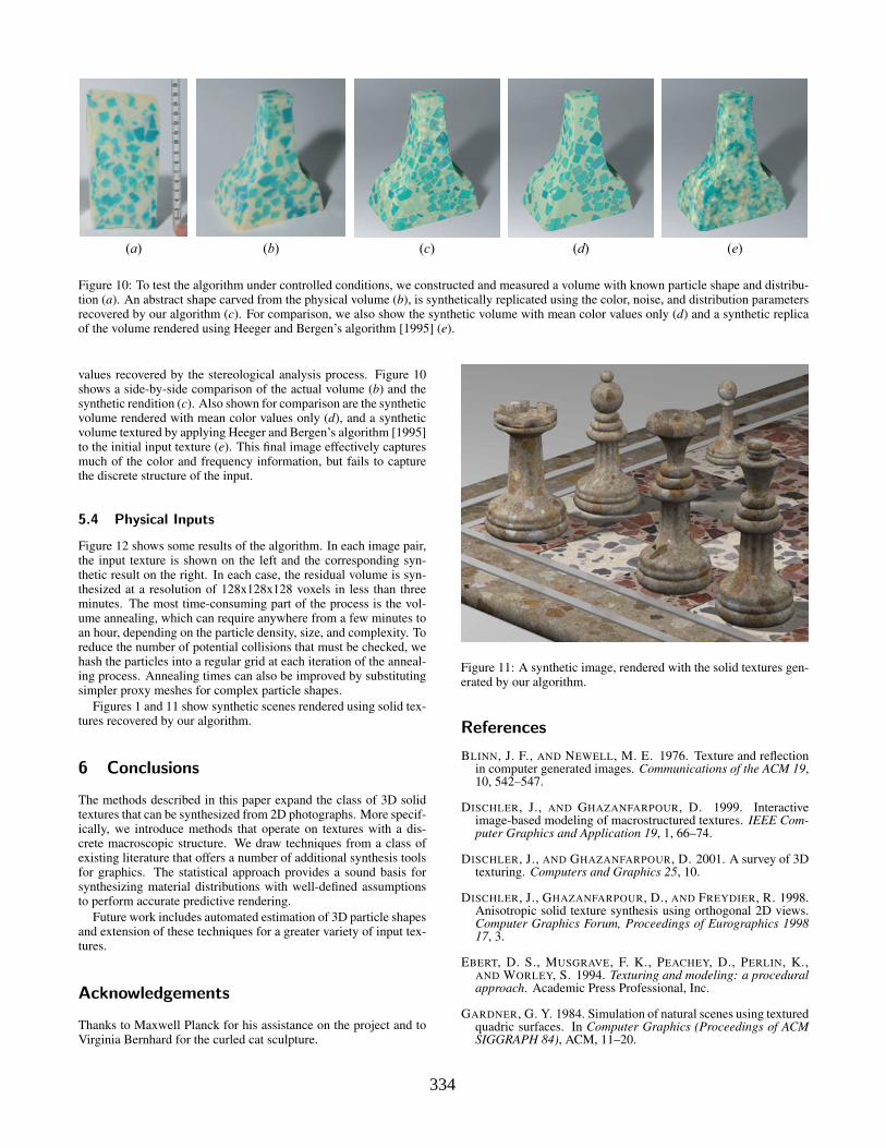
Figure 10: To test the algorithm under controlled conditions, we constructed and measured a volume with known particle shape and distribu-tion (a). An abstract shape carved from the physical volume (b), is synthetically replicated using the color, noise, and distribution parametersrecovered by our algorithm (c). For comparison, we also show the synthetic volume with mean color values only (d) and a synthetic replicaof the volume rendered using Heeger and Bergen’s algorithm [1995] (e).

values recovered by the stereological analysis process. Figure 10shows a side-by-side comparison of the actual volume (b) and thesynthetic rendition (c). Also shown for comparison are the syntheticvolume rendered with mean color values only (d), and a syntheticvolume textured by applying Heeger and Bergen’s algorithm [1995]to the initial input texture (e). This final image effectively capturesmuch of the color and frequency information, but fails to capturethe discrete structure of the input.

5.4 Physical Inputs

Figure 12 shows some results of the algorithm. In each image pair,the input texture is shown on the left and the corresponding syn-thetic result on the right. In each case, the residual volume is syn-thesized at a resolution of 128x128x128 voxels in less than threeminutes. The most time-consuming part of the process is the vol-ume annealing, which can require anywhere from a few minutes toan hour, depending on the particle density, size, and complexity. Toreduce the number of potential collisions that must be checked, wehash the particles into a regular grid at each iteration of the anneal-ing process. Annealing times can also be improved by substitutingsimpler proxy meshes for complex particle shapes.

Figures 1 and 11 show synthetic scenes rendered using solid tex-tures recovered by our algorithm.

6 Conclusions

The methods described in this paper expand the class of 3D solidtextures that can be synthesized from 2D photographs. More specif-ically, we introduce methods that operate on textures with a dis-crete macroscopic structure. We draw techniques from a class ofexisting literature that offers a number of additional synthesis toolsfor graphics. The statistical approach provides a sound basis forsynthesizing material distributions with well-defined assumptionsto perform accurate predictive rendering.

Future work includes automated estimation of 3D particle shapesand extension of these techniques for a greater variety of input tex-tures.

Acknowledgements

Thanks to Maxwell Planck for his assistance on the project and toVirginia Bernhard for the curled cat sculpture.

Figure 11: A synthetic image, rendered with the solid textures gen-erated by our algorithm.

References

BLINN, J. F., AND NEWELL, M. E. 1976. Texture and reflectionin computer generated images. Communications of the ACM 19,10, 542–547.

DISCHLER, J., AND GHAZANFARPOUR, D. 1999. Interactiveimage-based modeling of macrostructured textures. IEEE Com-puter Graphics and Application 19, 1, 66–74.

DISCHLER, J., AND GHAZANFARPOUR, D. 2001. A survey of 3Dtexturing. Computers and Graphics 25, 10.

DISCHLER, J., GHAZANFARPOUR, D., AND FREYDIER, R. 1998.Anisotropic solid texture synthesis using orthogonal 2D views.Computer Graphics Forum, Proceedings of Eurographics 199817, 3.

EBERT, D. S., MUSGRAVE, F. K., PEACHEY, D., PERLIN, K.,AND WORLEY, S. 1994. Texturing and modeling: a proceduralapproach. Academic Press Professional, Inc.

GARDNER, G. Y. 1984. Simulation of natural scenes using texturedquadric surfaces. In Computer Graphics (Proceedings of ACMSIGGRAPH 84), ACM, 11–20.

334

Figure 12: In each image pair, physical inputs to the solid texture algorithm are shown on the left and synthetic results are shown on the right.

GORLA, G., INTERRANTE, V., AND SAPIRO, G., 2001. Growingfitted textures. ACM SIGGRAPH 2001 Sketches and Applica-tions, August.

HAGWOOD, C. 1990. A mathematical treatment of the sphericalstereology. NISTIR 4370 (July), 1–17.

HEEGER, D. J., AND BERGEN, J. R. 1995. Pyramid-based tex-ture analysis/synthesis. In Proceedings of ACM SIGGRAPH2001, Computer Graphics Proceedings, Annual Conference Se-ries, ACM, 229–238.

HOWARD, C., AND REED, M. 1998. Unbiased Stereology.Springer-Verlag.

KEIDING, N., AND JENSEN, S. T. 1972. Maximum likelihood es-timation of the size distribution of liver cell nuclei from the ob-served distribution in a plane section. Biometrics 28, 3 (Septem-ber), 813–829.

LEFEBVRE, L., AND POULIN, P. 2000. Analysis and synthesis ofstructural textures. In Graphics Interface 2000, 77–86.

MAERZ, N. H. 1996. Reconstructing 3-D block size distribu-tions from 2-D measurements on sections. In Proceedings of theFRAGBLAST 5 Workshop on Measurement of Blast Fragmenta-tion, 39–43.

PEACHEY, D. R. 1985. Solid texturing of complex surfaces.In Computer Graphics (Proceedings of ACM SIGGRAPH 85),ACM, 279–286.

PERLIN, K. 1985. An image synthesizer. In Computer Graphics(Proceedings of ACM SIGGRAPH 85), ACM, 287–296.

SALTIKOV, S. A. 1967. The determination of the size distributionof particles in an opaque material from a measurement of thesize distribution of their sections. In Proceedings of the SecondInternational Congress on Stereology, 163–173.

TURK, G. 2001. Texture synthesis on surfaces. In Proceedings ofACM SIGGRAPH 2001, Computer Graphics Proceedings, An-nual Conference Series, ACM, 347–354.

UNDERWOOD, E. E. 1970. Quantitative Stereology. Addison-Wesley.

WEI, L., AND LEVOY, M. 2001. Texture synthesis over arbi-trary manifold surfaces. In Proceedings of ACM SIGGRAPH2001, Computer Graphics Proceedings, Annual Conference Se-ries, ACM, 355–360.

WEI, L. 2001. Texture Synthesis by Fixed Neighborhood Search-ing. PhD thesis, Stanford University.

WEI, L., 2003. Texture synthesis from multiple sources. ACMSIGGRAPH 2003 Sketches & Applications, July.

WOJNAR, L. 2002. Stereology from one of all the possible angles.Image Analysis and Stereology 21, Supplement 1, S1–S11.

335