stellar spectral models compared with empirical dataclok.uclan.ac.uk/27861/8/27861 stz754...
TRANSCRIPT
Article
Stellar spectral models compared with empirical data
Knowles, Adam T, Sansom, Anne E, Coelho, P R T, Prieto, C Allende, Conroy, C and Vazdekis, A
Available at http://clok.uclan.ac.uk/27861/
Knowles, Adam T, Sansom, Anne E ORCID: 0000000227827388, Coelho, P R T, Prieto, C Allende, Conroy, C and Vazdekis, A (2019) Stellar spectral models compared with empirical data. Monthly Notices of the Royal Astronomical Society, 486 (2). pp. 18141832. ISSN 00358711
It is advisable to refer to the publisher’s version if you intend to cite from the work.http://dx.doi.org/10.1093/mnras/stz754
For more information about UCLan’s research in this area go to http://www.uclan.ac.uk/researchgroups/ and search for <name of research Group>.
For information about Research generally at UCLan please go to http://www.uclan.ac.uk/research/
All outputs in CLoK are protected by Intellectual Property Rights law, includingCopyright law. Copyright, IPR and Moral Rights for the works on this site are retained by the individual authors and/or other copyright owners. Terms and conditions for use of this material are defined in the http://clok.uclan.ac.uk/policies/
CLoKCentral Lancashire online Knowledgewww.clok.uclan.ac.uk

MNRAS 486, 1814–1832 (2019) doi:10.1093/mnras/stz754Advance Access publication 2019 March 15
Stellar spectral models compared with empirical data
Adam T. Knowles ,1‹ A. E. Sansom ,1 P. R. T. Coelho,2 C. Allende Prieto,3,4
C. Conroy5 and A. Vazdekis 3,4
1Jeremiah Horrocks Institute, School of Physical Sciences and Computing, University of Central Lancashire, Preston PR1 2HE, UK2Instituto de Astronomia, Geofısica e Ciecias Atmosfericas, Univ. de Sao Paulo, Rua do Matao 1226, 05508-090 Sao Paulo, Brazil3Instituto de Astrofısica de Canarias, Vıa Lactea, E-38205 La Laguna, Tenerife, Spain4Universidad de La Laguna, Departamento de Astrofısica, E-38206 La Laguna, Tenerife, Spain5Department of Astronomy, Harvard University, Cambridge, MA 02138, USA
Accepted 2019 March 1. Received 2019 February 1; in original form 2018 May 25
ABSTRACTThe empirical MILES stellar library is used to test the accuracy of three different, state-of-the-art, theoretical model libraries of stellar spectra. These models are widely used in the literaturefor stellar population analysis. A differential approach is used so that responses to elementalabundance changes are tested rather than absolute levels of the theoretical spectra. First wedirectly compare model line strengths and spectra to empirical data to investigate trends. Thenwe test how well line strengths match when element response functions are used to accountfor changes in [α/Fe] abundances. The aim is to find out where models best represent realstar spectra, in a differential way, and hence identify good choices of models to use in stellarpopulation analysis involving abundance patterns. We find that most spectral line strengths arewell represented by these models, particularly iron- and sodium-sensitive indices. Exceptionsinclude the higher order Balmer lines (Hδ, Hγ ), in which the models show more variationthan the data, particularly at low temperatures. C24668 is systematically underestimated by themodels compared to observations. We find that differences between these models are generallyless significant than the ways in which models vary from the data. Corrections to C2 line listsfor one set of models are identified, improving them for future use.
Key words: techniques: spectroscopic – stars: abundances – stars: atmospheres.
1 IN T RO D U C T I O N
Element abundance patterns in galaxies are well known to containinformation about the formation history of their constituent stellarpopulations (e.g. Worthey, Faber & Gonzalez 1992; Proctor &Sansom 2002; Trager et al. 2000; Thomas et al. 2005). Evenmedium-resolution spectra of galaxies contain detailed informationregarding abundance patterns. The dominant sources of interstellarmedium (ISM) enrichment are Type II and Type Ia supernovae.Supernovae from massive star progenitors enrich the ISM with arange of heavy elements over time-scales of less than 108 yr. TypeIa supernovae, from white dwarf progenitors, enrich the ISM withmainly iron-peak elements over longer time-scales, ranging fromprompt explosions of ≈108 yr to a more delayed enrichment of up to≈1010 yr (Sullivan et al. 2006; Mannucci 2008; Pagel 2009; Maoz,Sharon & Gal-Yam 2010). The time-scales of elemental productionin the two types of supernovae are different; therefore, it is possibleto use the ratio of α-capture and iron-peak elements (e.g. from
� E-mail: [email protected]
observations of [Mg/Fe]1) as a clock to constrain the time-scaleover which the stars were born. Abundance patterns in galaxiescan be measured using spectral indices or full spectrum fitting. Wedescribe these two approaches below.
One way to measure abundance ratios from observing integratedpopulations is to measure spectral indices and compare with modelvalues. Commonly, such indices are defined by three bandpasses,a feature band and two sidebands (pseudocontinua), and are thenmeasured as a pseudo-equivalent width. The most popular systemof indices is the LICK/IDS system (e.g. Worthey 1994; Worthey &Ottaviani 1997) that defines 25 spectral indices between 4000 and6500 Å, although other systems have been designed for use withspectral libraries at different spectral resolutions, e.g. the Line IndexSystem (LIS) MILES system (Vazdekis et al. 2010). There are otherways to define indices, such as flux ratio indices (Rose 1984) orindices based on the D4000 feature (Poggianti & Barbaro 1997).With an index system defined, it can be used to investigate theproperties of stellar populations in galaxies. Moreover, it is possible
1[A/B] = log [n(A)/n(B)]∗ - log [n(A)/n(B)]�, where n(A)/n(B) is the numberabundance ratio of element A, relative to element B.
C© 2019 The Author(s)Published by Oxford University Press on behalf of the Royal Astronomical Society
Dow
nloaded from https://academ
ic.oup.com/m
nras/article-abstract/486/2/1814/5381560 by University of C
entral Lancashire user on 30 April 2019
Stellar spectral models compared with empirical data 1815
to study how the indices respond to elemental abundance changesusing theoretically produced stellar spectra. The results are usuallypresented in the form of response functions, which are tables thatshow how spectral features are affected by abundance changes.This type of study was first performed in the work of Tripicco &Bell (1995) with the assessment of 10 elements using syntheticspectra. A developed version of this study, whose derived responsefunctions have been widely used to date, was then carried out byKorn, Maraston & Thomas (2005). They used updated linelistsand atomic transition probabilities with more accurate atmosphericmodels and also incorporated a range of metallicities. Sansom et al.(2013) tested the differential behaviour of the Korn et al. (2005)models, via response functions and found deviations in the higherorder Balmer features between those models and empirical stardata. More updated and larger numbers of theoretical spectra havebeen used in more recent studies (e.g. Lee et al. 2009; Holtzmanet al. 2015). With measures of how spectral indices are sensitive toelemental abundances, one can use the derived response functionsto differentially correct indices to account for changes in abundancepatterns. There are many applications of such work throughout theliterature in both Milky Way and extragalactic studies (e.g. Trageret al. 2000; Proctor & Sansom 2002; Schiavon 2007; Thomas,Johansson & Maraston 2011; Onodera et al. 2015; Sesto et al.2018).
Another approach to account for different abundance patterns isfull spectrum fitting. Some of the first work to take a differentialabundance pattern approach in full spectrum fitting of stellarpopulations was that of Prugniel et al. (2007) followed by thatof Walcher et al. (2009), for the modelling of α-enhanced SimpleStellar Populations (SSPs). This work was then expanded byConroy & van Dokkum (2012), by varying 11 elements separately.Vazdekis et al. (2015) performed a similar approach to Walcher et al.(2009), focusing on an α enhancement in SSPs. A similar methodfor differentially correcting individual star spectra can be used toaccount for variations in abundance patterns. If accurate measuresare made that quantify how spectral indices or full spectra respond toelemental abundances, it is possible to begin to build stellar spectrallibraries that contain abundance patterns different from our ownsolar neighborhood. Such libraries allow one to produce stellarpopulation synthesis models that include stars with abundancepatterns that differ from the Milky Way. This is motivated by thedifferent abundance patterns seen in giant Early-Type and DwarfSpheroidal galaxies (e.g. Letarte, Hill & Tolstoy 2007; Conroy,Graves & van Dokkum 2014).
Differentially correcting empirical stellar spectra relies on theaccuracy of the theoretical stellar spectra used. With a large numberof models currently available, each with their own set of advantages,assumptions, and limitations, deciding which synthetic spectrato use is difficult. Here we test the predictions of three stellarspectral model libraries against empirical star data in the context ofabundance patterns, with the aim of highlighting current strengthsand weaknesses of the models. These models represent some of themost recent works in stellar population analysis, covering a broadrange of parameter space, suitable for modelling integrated stellarpopulations. This work expands on Sansom et al. (2013), testingmore state-of-the-art theoretical stellar spectral models.
The structure for this paper is as follows. Section 2 describes thethree models of stellar spectra that are tested in this study. Section3 outlines the MILES empirical spectra used in the comparison.In Section 4 we directly compare Lick indices of MILES stars tothose predicted from theoretical stellar spectra. Section 5 presentsa differential approach, using response functions, in which we
compare normalized Lick indices from empirical MILES starsto those predicted from theoretical response functions. Section 6discusses the findings and possible physical reasons for modeldisagreements, through analysis of both indices and full spectra.Section 7 presents our conclusions.
2 MODELS OF STELLAR SPECTRA
Throughout this paper we will be using three model librariesof stellar spectra, produced by three independent authors to testresponses of the models to changes in abundance pattern, relativeto solar. The models we have chosen are state-of-the-art in thecontext of stellar population analyses from integrated light. Theyhave been created for use in stellar population modelling, coveringa wide range of stellar parameters and abundance patterns. Somerecent works applying these models can be found in Conroy et al.(2014), Holtzman et al. (2015), and Vazdekis et al. (2015). Thesemodels built on the first predictions of SSP spectra with abundancevariations from the works of Coelho et al. (2007), Prugniel et al.(2007), Percival et al. (2009), and Lee et al. (2009). All of theseworks predict the spectra of stellar populations with abundancevariations, rather than the classical approach of predicting indices.This section describes and outlines the codes and parameters usedin the production of the theoretical stellar spectra from each of threemodellers.
Generation of synthetic spectra requires two main steps. First,calculation of the model atmosphere provides a mathematical modeldescribing the variation of physical parameters such as density,temperature, and pressure as a function of radial depth, for anassumed star type and composition. The second step is to passphotons through the generated atmosphere to compute an emergentspectrum. This requires the use of a synthetic spectrum codetogether with a list of line and molecular absorption transitionsand a specification of element abundances. The self-consistentapproach to generate a theoretical stellar spectrum would be toexactly match the abundances in both steps of the production. Toreduce computational time, a simplification is made in which onlythe dominant sources of opacity are varied in the model atmospherewhilst more elements are varied in the synthetic spectrum. Howeverif one uses ATLAS12 (Kurucz 1996) or OMARCS (Gustafssonet al. 2008) model atmosphere codes, it is possible to have the sameabundance pattern in both components of the spectrum generation.
One of the most commonly used codes to generate model atmo-spheres is ATLAS (Kurucz 1979 and updates), a one-dimensional,local thermodynamic equilibrium and plane-parallel code. Theoriginal code provides a base on which developments have beenmade, e.g. ATLAS9 (Kurucz 1993) and ATLAS12 (Kurucz 2005;Castelli 2005a). An important effect in the generation of stellarphotospheres is the line opacity due to atomic (and molecular) lineabsorption. Line opacity depends on temperature, pressure, chem-ical composition, and microturbulence (vturb). Statistical methodswere developed to deal with the vast number of lines present instellar atmospheres. The method implemented provides one of thebiggest differences between the versions of the ATLAS code. ATLAS9uses Opacity Distribution Functions (ODFs) as an approach to thisproblem. ODFs treat the line opacities in a given frequency intervalby a smoothly varying function. The ODFs have to be computedfor a particular abundance pattern before generating the modelatmospheres. ATLAS12 uses the Opacity Sampling method (OS)to compute the line opacity at a number of frequency points.
Another important parameter in the computation of stellar spectrais vturb. This microturbulence has a large impact on strong or
MNRAS 486, 1814–1832 (2019)
Dow
nloaded from https://academ
ic.oup.com/m
nras/article-abstract/486/2/1814/5381560 by University of C
entral Lancashire user on 30 April 2019

1816 A. T. Knowles et al.
saturated lines, and therefore the choice of this parameter when cal-culating a synthetic spectrum will affect the resulting line strengths.In order to gain an understanding of line-strength uncertaintiesinvolved with the vturb parameter, we produced several modelschanging vturb (see Section 4).
In this paper we test three star types with varying elementabundances that represent Cool Dwarf (CD) (Teff = 4575 K, logg = 4.60 dex), Cool Giant (CG) (Teff = 4255 K, log g = 1.90 dex),and Turn-off (TO) (Teff = 6200 K, log g = 4.10) stars with the sameparameters as in Korn et al. (2005) and the analysis of Sansom et al.(2013). These star types are chosen as they are representative ofstars present in older stellar populations that future work will focuson, using results from this study.
Below we specify the codes used by the three modellers toproduce spectra, the wavelength range, sampling, elements varied,and stellar parameters used. Table 1 summarizes this information.All models assume that the α-capture group elements are O, Ne,Mg, Si, Ca, and Ti, unless otherwise stated. Spectra with abundancepatterns of Solar and those in Table 2 were provided. Table 2summarizes the Teff, log g, and element enhancements providedby each modeller, for use in Section 5. The [M/H] value in Table 2is defined as a scaled metallicity.
2.1 Conroy
Theoretical star spectra from Conroy were made using the ATLAS12atmosphere code and SYNTHE (Kurucz & Avrett 1981) spectralsynthesis package. Groups of Cool Dwarf, Cool Giant, and Turn-offstar spectra were made with a wavelength range of 3700–10000 Åand sampling of �log λ(Å) = 2.17 × 10⁻⁵. It is worth highlightinghere that only spectra with a C+0.15 dex variation (compared withC + 0.3 dex of the other two authors) were provided, which willimpact on the derived responses for indices that are particularlysensitive to carbon abundances. The reason for this was to avoidthe generation of carbon stars. The solar abundances adopted inthe model atmosphere and synthetic spectrum code were fromAsplund et al. (2009). Note that the stellar parameters used inproducing the model atmospheres were slightly different from theparameters of the other two modellers. This was because thesemodels already existed prior to the current work, rather than beingcreated specifically for this project (as in the other two cases).Further description of the stellar spectral models can be found inConroy & van Dokkum (2012). Please note that the native resolutionand wavelength range of the models presented in Conroy & vanDokkum (2012) is higher than that given in Table 1, but the spectrawere downsampled and cut at 10 000 Å. The line lists used in theproduction of Conroy’s models are described in Conroy & vanDokkum (2012) and are based on lists compiled by Kurucz.2 Someof the differences between the three models seen in Sections 4 and5 may be explained by the inclusion of predicted lines (PLs) inConroy models that are not present in the other two model libraries.The PLs were included in the Conroy models provided becausethere were generated for other applications, particularly to computebroad-band colours, which are known to be underestimated if PLsare missing (e.g. section 3 of Coelho 2014 and section 3.2 of Coelhoet al. 2007). Most of the PLs are weak, and therefore contribute tothe overall continuum shape. However, there are cases of strongPLs that produce lines that disagree with observations, particularlyin the bluer parts of the spectrum (see bottom panel of figs 2 and
2http://kurucz.harvard.edu
3 of Munari et al. 2005 as well as figs 7–18 of Bell, Paltoglou &Tripicco 1994). The PLs affect the absolute comparisons more thanthe differential comparisons.
2.2 Coelho
Theoretical star spectra provided by Coelho used both the ATLAS12model atmosphere code and SYNTHE (Kurucz & Avrett 1981;Sbordone et al. 2004) spectral synthesis code to generate groups ofspectra for a Cool Dwarf, Cool Giant, and Turn-off star. The originalwavelength range of the spectra was 3000–8005 Å with a samplingof �log λ(Å) = 1.4 × 10⁻⁶. The solar abundances used in the modelatmosphere and synthetic spectrum code were those of Grevesse &Sauval (1998). These models are different from those previouslypublished by Coelho, which were based on ATLAS9 (Coelho 2014).The atomic line lists used in Coelho’s models are a combinationof lists from Coelho et al. (2005), Castelli (2005a), and Castelli(2005b). In this work we adopt the same molecular opacities as inCoelho (2014), with the following updates3: C2 D-A (from Brookeet al. 2013), CH (from Johnson et al. 2014, with energy levelssubstituted from Zachwieja 1995; Zachwieja 1997; Colin & Bernath2010; Bembenek, Kepa & Rytel 1997; Kepa et al. 1996), and CNA-X and B-X (from Brooke et al. 2014). During the progress of thiswork, we identified that the file regarding the transition D-A of themolecule C2 used in Coelho (2014) was corrupted. We thereforewarn that the predictions of that library around the main C2 featuresshould be taken with care. This is illustrated in Appendix A, wherewe compare the corrupted and corrected models. This corruption islikely to be the origin of the strong missing opacity around 4000Å in the second panel of fig. 10 in Coelho (2014), which can beattributed to Swan Bands. Note that this problem did not affectearlier models, including Coelho et al. (2005), Coelho et al. (2007),or Vazdekis et al. (2015).
2.3 Allende prieto
The spectra provided by Allende Prieto (hereafter referred to asCAP) were made using the ATLAS9 model atmosphere code alongwith the ASSεT (Koesterke 2009) spectral synthesis software, usedin 1-D. The wavelength range of the spectra was 1200–300 00 Åwith a sampling of �log λ(Å) = 6.5 × 10⁻⁷. The solar abundanceused in both the model atmosphere and synthetic spectrum codewas that of Asplund et al. (2005). Further details of the models canbe found in Allende Prieto et al. (2014). The line lists used in theCAP models are detailed in Meszaros et al. (2012) and are basedon Kurucz lists.
For the CAP models that we generate for Section 4, we useATLAS9. We direct interested readers to Meszaros et al. (2012) andweb pages for the ATLAS-APOGEE survey analysis4 for furtherinformation on the ODFs and models used in this analysis. Currentlyfor PL9, the ODFs publicly available from the ATLAS-APOGEEwebsite provide a range of abundances in [M/H], [α/M], and [C/M].[M/H] here is defined as a scaled metallicity. This definition meanselements with Z > 2 are all scaled together e.g. [M/H] = 0.2 means[Fe/H] = 0.2 = [X/H], where X = 3,4, ..., 99. Note that with thesedefinitions, [M/H] represents all elements other than the α-capture
3As made available by R. Kurucz; downloaded on 2016 December fromhttp://kurucz.harvard.edu/molecules.html4http://www.iac.es/proyecto/ATLAS-APOGEE/
MNRAS 486, 1814–1832 (2019)
Dow
nloaded from https://academ
ic.oup.com/m
nras/article-abstract/486/2/1814/5381560 by University of C
entral Lancashire user on 30 April 2019

Stellar spectral models compared with empirical data 1817
Table 1. Codes and parameters used by the three modellers when generating their theoretical spectra. These parameters are for spectra used in the derivationof response functions in Section 5. In the final column we specify the consistency of abundance specification between the model atmosphere (MA) generationand radiative transfer (RT) process.
ModelAtmospherecode
Syntheticspectrum code
Wavelengthrange (Å)
Sampling(�log λ(Å)) vturb (km/s) Solar abundance reference
MA + RTcompatible
Conroy ATLAS12 SYNTHE 3700-10000 2.17 × 10⁻⁵ 2 Asplund et al. (2009) YesCoelho ATLAS12 SYNTHE 2995-8005 1.4 × 10⁻⁶ 2 Grevesse & Sauval (1998) YesAllende Prieto(CAP)
ATLAS9 ASSεT 1200-30000 6 × 10⁻⁷ 1.5 Asplund, Grevesse &Sauval (2005)
Yes (C, M, α)
Table 2. Teff, Log g, and element enhancements above solar (0.3 dex unless stated otherwise) for the three star types, provided by the modellers for theresponse function analysis in Section 5. The [M/H] column in this table is for the specific case of all metals increased by 0.3 dex.
Model Teff (CD,CG,TO) (K) Log g (CD,CG,TO) (dex) C N O Mg Fe Ca Na Si Cr Ti [M/H]
Conroy 4500,4250,6150 4.60,1.94,4.06 �(0.15dex)
� x � � � � � � � �
Coelho 4575,4255,6200 4.60,1.90,4.10 � � � � x � x x x x �
CAP 4575,4255,6200 4.60,1.90,4.10 � � � � � � � � � � �
elements if there is an α enhancement or deficiency (e.g. if [M/H] =0.2 and [α/M] = 0.1, this means that [α/H] = 0.3 and [Fe/H] = 0.2).
3 EMPIRICAL STELLAR SPECTRA
The empirical data are from the Medium resolution Isaac NewtonLibrary of Empirical Spectra (MILES) (Sanchez-Blazquez et al.2006). Whilst stars from our Galaxy do not cover the full parameterrange of stars in other galaxies, they do cover a broad range instellar parameters. These empirical spectra have a wavelength rangeof 3500–7500Å, resolution (FWHM) of 2.5 Å, and sampling of0.9 Å (Falcon-Barroso et al. 2011). They have a typical signal-to-noise ratio of over 100 Å−1, apart from stars that are members ofglobular clusters. Of the 985 stars in MILES, Milone, Sansom &Sanchez-Blazquez (2011) measured the [Mg/Fe] abundances for752 stars. We use their [Mg/Fe] measurement as a proxy for all[α/Fe] abundances in these stars. Therefore MILES is a stellarlibrary for which we know attributes of effective temperature (Teff),surface gravity (log g), metallicity ([Fe/H]), and abundance ratios([α/Fe]) for a large proportion of the whole library. This, with theMILES spectra, allows us a uniformly calibrated data set of starsto test theoretical spectra. We initially use a sub-sample of 51 ofthe 752 stars that matched the Teff and log g parameters of the threetheoretical stars described in Section 2, within the observationalerrors. Stars were chosen that were within �Teff ≤ ± 100 K, �logg ≤ ± 0.2) of the Cenarro et al. (2007) atmospheric parameters,for three specific star types. These limits led to a sample of 7 CoolDwarfs, 13 Cool Giants, and 31 Turn-off stars (see Sansom et al.2013, table A1 for details of these individual star parameters andLick indices). Therefore we have both MILES spectra and their Lickindices available for testing. Whilst full spectrum fitting has becomeincreasingly popular for stellar population analysis in recent years,Lick indices are useful for testing properties of theoretical spectraagainst observations because they focus on the strongest spectralfeatures. We use the Teff, log g, [Fe/H], and [Mg/Fe] values of theMILES stars presented in table A1 of Sansom et al. (2013), basedon parameters in Cenarro et al. (2007), unless stated otherwise.The errors on the measured MILES Lick indices were computed bySanchez-Blazquez (private communication), from the error spectraobtained by propagating uncertainties throughout the reductions,
including flux and wavelength calibration, as well as the errors inthe velocity calculations, for each star.
4 D I R E C T C O M PA R I S O N S
The first test we perform directly compares MILES and theoreticalstar Lick indices. New models are generated that match the MILESstars exactly in Teff, log g, [Fe/H], and [α/Fe] for Coelho andCAP models. The theoretical spectra were degraded to the MILESresolution of FWHM = 2.5 Å (Falcon-Barroso et al. 2011) using aconvolution code produced in PYTHON and then resampled to matchexisting MILES sampling of 0.9 Å. Indices are then measured forboth the MILES stars and corresponding theoretical star using LEC-TOR software (Vazdekis 2011). This approach of directly producingmodels was made for both the Coelho and CAP models, to compareto the sub-sample of 51 MILES stars, described in Section 3. Ratherthan generating models directly for this comparison, spectra werecreated for Conroy models using an interpolation within a pre-existing grid presented in Conroy & van Dokkum (2012). Four ofthe 51 MILES stars fell outside of the parameter range in the gridand were therefore not modelled for Conroy in this comparison. Themissing stars were three Turn-off stars (HD084937, HD338529, andBD + 092190) and one cool giant star (HD131430). Although thisdirect comparison will assess the absolute behaviour of models,the main purpose of this test is to look for trends between modelsrather than absolute agreement between models and empirical data.The absolute test we perform here will aid the assessment of thedifferential test performed in Section 5.
The available measured MILES star parameters are Teff, log g,[Fe/H], and [Mg/Fe]. CAP models are generated by specifying Teff,log g, [M/H], [α/M], and [C/M] and vturb. Therefore, conversionsfrom MILES parameters to the model parameters are required, inaddition to assumptions of [C/M] and vturb for the empirical stars.The choice of vturb to use in the models is explained in Section 4.1and the conversion process is described in Section 4.2.
4.1 Microturbulent velocity
To investigate the effects of microturbulent velocity on the differ-ential application of theoretical line-strengths, three different star
MNRAS 486, 1814–1832 (2019)
Dow
nloaded from https://academ
ic.oup.com/m
nras/article-abstract/486/2/1814/5381560 by University of C
entral Lancashire user on 30 April 2019

1818 A. T. Knowles et al.
models were produced using the codes of Allende Prieto et al.(2014). For each base star type (Cool Dwarf, Cool Giant, and Turn-off), we produced an [α/M] =0.25 dex and a [α/M]=0 dex spectrumat vturb = 1 km s−1 (v1) and 2 km s−1 (v2) . All the models wereproduced with the same sampling of �log λ(Å) = 0.025 Å (at 3000Å) to isolate the effects of vturb. The models were blurred to MILESFWHM of 2.5 Å and resampled to MILES linear sampling of 0.9Å using the same procedure as described previously. LECTOR wasthen used to compute the line strengths. To assess the differentialeffect, we took a difference of line strengths through:(
v2
([α
M
]= 0.25
)− v2(�)
)
−(
v1
([α
M
]= 0.25
)− v1(�)
), (1)
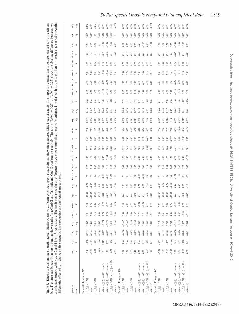
where vi represents the spectrum with vturb = i km s−1 and indicesare measured from these model spectra. Table 3 shows the line-strength indices measured for each of the models as well as thedifferential effects.
In general, the effect of vturb on the Cool Dwarf line strengths issmallest, with typical differences of 0.2 Å between 1 and 2 km s−1,respectively. The microturbluent velocity has a far greater effect onthe Cool Giant spectra with several features differing by order ∼1–2 Å, particularly Hγ A, G4300, and Fe5015, with a change in vturb
from 1 km s−1 to 2 km s−1. The Turn-off stars are also significantlyaffected by vturb. For all star types the differential vturb effect issmall; as can be seen in the v2(δ)-v1(δ) of Table 3. Our findingsshow that these differences are generally much smaller (∼0.02 dex;see Table 3.) than the observational errors on line strengths (∼0.1dex; see table 2 of Sansom et al. 2013)
For simplicity, we have chosen to use a constant value ofvturb = 1.5 kms−1 for all our models used in this paper, unlessotherwise stated. This choice is motivated by larger studies of stars inour Galaxy, where vturb is measured between the 1 and 2 kms−1 (e.g.Holtzman et al. 2015).
4.2 Abundances in CAP models
Two approximations are made in the format conversion process forelement abundances. First, it is assumed that [Mg/Fe] is a proxyfor [α/Fe]. This is a reasonable assumption for solar neighbourhoodstars, like the 51 MILES stars used in this study, as is shown by thework of Delgado Mena et al. (2010) and Holtzman et al. (2015).A second approximation of [C/Fe] = 0 for the MILES stars wasmade based on results from da Silva, Milone & Reddy (2011) andHoltzman et al. (2015) for stars in our Galaxy.
The [Mg/Fe] and [Fe/H] abundances of the MILES stars arematched in the generated CAP model through [α/M] and [M/H],respectively. Therefore we use the assumption that [Fe/H]≈[M/H]and [Mg/Fe]≈[α/M]. [C/Fe] values of the MILES stars are assumedto be 0 throughout, meaning that [C/M] = 0 in the generated models.For these CAP models, solar abundances are defined on the Asplundet al. (2005). Using these conversions, spectra are generated in a self-consistent way, with the abundances of α and C varied in the sameway for both model atmosphere and spectral synthesis calculations.
4.3 Absolute comparisons
Figs 1–5 show direct comparisons between the measured MILESLick indices and corresponding model Lick indices for these MILESmatched spectra.
Fig. 1 shows that the absolute line strengths of the higherorder Balmer lines and Hβ for Conroy, Coelho, and CAP modelsdeviate from observations and this effect increases towards morenegative line strengths and cooler temperatures. Fig. 2 shows thatConroy, Coelho, and CAP models predict iron-sensitive featuresqualitatively well in the absolute comparison, with no strongsystematic deviations from the 1:1 agreement lines. Fig. 3 shows agood agreement, over a broad range in index strengths, particularlyfor CAP models compared with observations for magnesium-sensitive features. There are slight overpredictions of line strengthsfor Coelho and CAP Cool Giant models, whilst the Conroy coolstar models overpredict these magnesium features the most, withclear systematic offsets. Fig. 4 shows that Conroy, Coelho, andCAP all underpredict the line strength indices in C24668 and showless variation than is present in MILES stars. Moreover, Conroyand CAP models overpredict the line strength indices of CN1 andCN2 for the cool stars. Fig. 5 shows the absolute predictions of theConroy, Coelho, and CAP models for calcium- and sodium-sensitiveindices agree well with the observations. However, differencesbetween models can be seen in the Ca4455 index, with Coelho CoolGiant models having a tighter relation to the 1:1 line and Conroymodels showing systematic overpredictions of this line strength.For Ca4227, the scatter is larger for the cool stars, with all threemodels behaving similarly. Despite the differences seen betweenmodels in Figs 1–5, it is interesting to note how similar the three setof models behave in general, given the different approaches, inputs,and codes of the three models. This tells us that the models areproducing similar predictions of the physical processes, althoughthere are still large differences between models and observations inabsolute terms.
5 R ESPONSE FUNCTI ONS AND THEI RAPPLI CATI ON
The results of Section 4 highlight the disagreements betweenthe models and MILES stars in absolute terms. Other studieshave also shown wavelength-dependent disagreements betweentheoretical models and observed spectra (e.g. Martins & Coelho2007; Bertone et al. 2008; Coelho 2014; Villaume et al. 2017;Allende Prieto et al. 2018). One method to incorporate both theabundance pattern predictions provided by theoretical models andthe reliability of empirical libraries is to use theoretical spectra todifferentially correct empirical spectra. Variations to Lick indices,due to changes in stellar atmospheric abundances, can be quantifiedin terms of response functions (Tripicco & Bell 1995). These canbe applied to change empirical or theoretical line-strengths dueto variations in abundance patterns, particularly differences fromsolar neighbourhood abundances. We produce response functiontables for the models of three star types: a Cool Dwarf, Cool Giant,and a Turn-off star, described in Section 2. To test the responsesof different theoretical models to abundance pattern changes, wecompare their normalized Lick indices predictions to measured Lickindices of existing MILES stars (described in Section 3).
We test the response functions, derived from theoretical spectraof the three star types, by applying them to a theoretical solarabundance pattern (base) star to account for changes in abundancepatterns, namely [α/Fe] changes. The base model star has the sameatmospheric parameters of Teff and log g as a chosen MILES basestar, within observational errors. The response functions will beused to modify Lick indices of the base model star to account foran abundance pattern of an existing MILES star with same Teff
and log g as the base star, referred to as an enhanced star. This
MNRAS 486, 1814–1832 (2019)
Dow
nloaded from https://academ
ic.oup.com/m
nras/article-abstract/486/2/1814/5381560 by University of C
entral Lancashire user on 30 April 2019
Stellar spectral models compared with empirical data 1819
Tabl
e3.
Eff
ects
ofv t
urb
onlin
e-st
reng
thin
dice
s.E
ach
row
show
sdi
ffer
entg
ener
ated
spec
tra
and
colu
mns
show
the
mea
sure
dL
ick
inde
xst
reng
ths.
The
impo
rtan
tcom
pari
son
isbe
twee
nth
ere
dro
ws
inea
chsu
bbo
x.T
heth
ree
sub-
boxe
s(f
rom
top
tobo
ttom
)sh
owre
sults
for
aC
oolG
iant
,Tur
n-of
f,an
dC
oolD
war
fst
ar,r
espe
ctiv
ely.
The
row
v2([
α/M
]=
0.25
)-v
1([
α/M
]=
0.25
)sh
ows
the
abso
lute
diff
eren
cebe
twee
ntw
oα
-enh
ance
dsp
ectr
aw
ithv t
urb
=2
and
1km
s−1,r
espe
ctiv
ely.
The
v2(δ
)-v
1(δ
)ro
wsh
ows
diff
eren
ces
betw
een
two
norm
aliz
edsp
ectr
a(α
-enh
ance
d–
sola
r)w
ithv t
urb
=2
and
1km
s−1.v
2(δ
)-v
1(δ
)in
red
show
sth
edi
ffer
entia
leff
ecto
fv t
urb
choi
ceon
line
stre
ngth
.Iti
ssh
own
that
the
diff
eren
tiale
ffec
tis
smal
l.
Spec
trum
Hδ
AH
δF
CN
1C
N2
Ca4
227
G43
00H
γA
Hγ
FFe
4383
Ca4
455
Fe45
31C
246
68H
βFe
5015
Mg 1
Mg 2
Mg b
Fe52
70Fe
5335
Fe54
06Fe
5709
Fe57
82N
a DT
iO1
TiO
2
Uni
tsÅ
Åm
agm
agÅ
ÅÅ
ÅÅ
ÅÅ
ÅÅ
Åm
agm
agÅ
ÅÅ
ÅÅ
ÅÅ
mag
mag
Tef
f=
4200
K,l
ogg
=2.
09
v1([
α M
]=
0.25)
−7.4
9−0
.38
0.23
50.
367
6.31
7.80
−12.
41−4
.70
8.59
2.22
5.15
3.37
0.66
7.80
0.19
30.
456
6.86
4.07
4.36
2.91
1.67
1.01
3.79
0.06
70.
136
v1(�
)−9
.09
−1.1
30.
314
0.44
15.
038.
36−1
2.33
−4.8
79.
392.
145.
013.
350.
337.
230.
184
0.38
75.
264.
274.
693.
091.
611.
144.
150.
032
0.08
3
v2([
α M
]=
0.25)
−8.2
7−0
.89
0.25
60.
411
6.16
8.76
−13.
30−4
.38
8.86
2.67
5.76
3.86
0.68
9.67
0.22
10.
477
6.58
4.67
5.22
3.31
2.06
1.34
3.79
0.07
0.14
6
v2(�
)−1
0.06
−1.6
60.
338
0.48
74.
889.
36−1
3.15
−4.5
19.
542.
575.
633.
830.
349.
180.
212
0.40
74.
974.
835.
543.
471.
991.
494.
50.
035
0.09
4
v1(δ
)=
v1([
α M
]=
0.25) −v
1(�
)1.
590.
746
−0.0
79−0
.074
1.28
−0.5
5−0
.08
0.17
−0.8
00.
080.
150.
020.
330.
570.
009
0.06
91.
60−0
.20
−0.3
3−0
.18
0.06
−0.1
3−0
.35
0.03
50.
053
v2(δ
)=
v2([
α M
]=
0.25) −v
2(�
)1.
790.
77−0
.082
−0.0
761.
28−0
.60
−0.1
50.
13−0
.68
0.11
0.13
40.
030.
350.
480.
009
0.07
01.
61−0
.16
−0.3
1−0
.16
0.07
−0.1
6−0
.36
0.03
50.
052
v2([
α M
]=
0.25)
−v1([
α M
]=
0.25)
−0.7
7−0
.50
0.02
10.
044
−0.1
50.
96−0
.89
0.32
0.27
50.
450.
610.
491
0.02
1.88
0.02
80.
021
−0.2
80.
590.
860.
390.
390.
33−0
.00
0.00
30.
01
v2(δ
)-v
1(δ
)0.
200.
03−0
.003
−0.0
020.
00−0
.04
−0.0
7−0
.03
0.12
0.03
−0.0
10.
010.
02−0
.08
0.00
00.
001
0.01
0.03
0.02
0.01
0.01
−0.0
20.
000
−0.0
01
Tef
f=
6253
K,l
ogg
=4.
28
v1([
α M
]=
0.25)
2.81
3.10
−0.1
00−0
.042
0.88
3.90
0.62
2.50
1.72
0.69
2.30
0.52
4.07
3.94
0.00
80.
088
2.37
1.82
1.87
0.80
0.52
0.25
0.67
0.00
20.
007
v1(�
)2.
592.
96−0
.097
−0.0
420.
664.
150.
282.
281.
910.
682.
150.
433.
963.
770.
008
0.07
31.
851.
671.
770.
790.
480.
230.
730.
002
0.00
6
v2([
α M
]=
0.25)
2.63
2.88
−0.0
92−0
.034
0.88
4.53
0.04
2.38
1.91
0.83
2.83
0.51
4.08
4.82
60.
011
0.09
22.
252.
072.
200.
930.
610.
270.
680.
002
0.00
8
v2(�
)2.
412.
73−0
.092
−0.0
350.
674.
75−0
.28
2.17
2.10
0.82
2.67
0.42
3.96
4.58
0.01
10.
077
1.73
1.89
2.07
0.93
0.57
0.26
0.75
0.00
20.
008
v1(δ
)=
v1([
α M
]=
0.25) −v
1(�
)0.
220.
14−0
.001
0.00
00.
22−0
.24
0.33
0.22
−0.1
90.
010.
110.
090.
110.
180.
000
0.01
50.
520.
160.
110.
010.
040.
01−0
.10.
000
0.00
1
v2(δ
)=
v2([
α M
]=
0.25) −v
2(�
)0.
220.
150.
000
0.00
10.
21−0
.21
0.31
0.22
−0.1
90.
000.
160.
090.
120.
240.
000
0.01
50.
520.
190.
130.
000.
050.
02−0
.07
0.00
00.
000
v2([
α M
]=
0.25) −v
1([
α M
]=
0.25)
−0.1
8−0
.22
0.00
60.
008
0.00
0.63
−0.5
8−0
.12
0.18
0.14
0.57
−0.0
120.
007
0.87
0.00
0.00
−0.1
20.
250.
320.
140.
090.
020.
000.
000
0.00
1
v2(δ
)−v
1(δ
)0.
00.
010.
001
0.00
1−0
.01
0.03
−0.0
20.
000.
000.
000.
100.
010.
010.
060.
000
0.00
00.
000.
030.
02−0
.01
0.01
0.00
−0.0
00.
000
−0.0
01
Tef
f=
4658
K,l
ogg
=4.
47
v1([
α M
]=
0.25)
−7.5
1−0
.32
0.09
20.
215
6.09
7.23
−11.
90−4
.32
8.21
12.2
84.
871.
350.
467.
040.
197
0.50
68.
214.
704.
863.
011.
220.
775.
290.
009
0.02
6
v1(�
)−9
.78
−1.3
70.
122
0.23
75.
018.
03−1
2.55
−4.7
69.
422.
234.
791.
470.
407.
000.
165
0.44
47.
114.
865.
203.
251.
180.
855.
770.
003
0.01
9
v2([
α M
]=
0.25)
−7.6
3−0
.39
0.10
00.
237
6.01
7.76
−12.
40−4
.26
8.26
2.54
5.35
1.66
0.40
7.97
0.21
40.
517
7.98
4.50
5.22
3.19
1.42
0.92
5.27
0.01
10.
031
v2(�
)−9
.92
−1.4
60.
128
0.25
54.
948.
54−1
2.97
−4.6
99.
402.
475.
281.
771
0.32
77.
980.
180.
456.
905.
135.
543.
41.
371.
015.
750.
004
0.02
4
v1(δ
)=
v1([
α M
]=
0.25) −v
1(�
)2.
271.
05−0
.030
−0.0
221.
08−0
.80
0.65
0.44
−1.2
10.
050.
08−0
.12
0.06
0.03
0.03
20.
062
1.10
−0.1
6−0
.34
−0.2
50.
04−0
.07
−0.4
80.
006
0.00
7
v2(δ
)=
v2([
α M
]=
0.25) −v
2(�
)2.
291.
07−0
.028
−0.0
181.
07−0
.79
0.58
0.43
−1.1
40.
070.
07−0
.11
0.07
−0.0
040.
035
0.06
31.
08−0
.13
−0.3
2−0
.23
0.05
−0.0
8−0
.48
0.00
70.
007
v2([
α M
]=
0.25) −v
1([
α M
]=
0.25)
−0.1
2−0
.08
0.00
80.
022
−0.0
80.
52−0
.50
0.06
0.05
0.27
0.48
0.31
−0.0
60.
940.
017
0.01
1−0
.23
0.30
0.36
0.18
0.20
0.15
−0.0
20.
002
0.00
5
v2(δ
)−v
1(δ
)0.
020.
020.
002
0.00
4−0
.01
0.01
−0.0
7−0
.01
0.07
0.02
−0.0
10.
010.
02−0
.04
0.00
30.
001
−0.0
60.
030.
020.
020.
01−0
.01
0.00
0.00
10.
000
MNRAS 486, 1814–1832 (2019)
Dow
nloaded from https://academ
ic.oup.com/m
nras/article-abstract/486/2/1814/5381560 by University of C
entral Lancashire user on 30 April 2019

1820 A. T. Knowles et al.
Figure 1. MILES Lick Indices versus Model Lick Indices, for Conroy, Coelho, and Allende Prieto (CAP) theoretical spectra that match the MILES atmosphericparameters given in Cenarro et al. (2007), for hydrogen-sensitive features. The three star types are shown in each case, with green, black, and red circlesrepresenting Turn-Off, Cool Dwarf, and Cool Giant stars, respectively.
MNRAS 486, 1814–1832 (2019)
Dow
nloaded from https://academ
ic.oup.com/m
nras/article-abstract/486/2/1814/5381560 by University of C
entral Lancashire user on 30 April 2019

Stellar spectral models compared with empirical data 1821
Figure 2. MILES Lick Indices versus Model Lick Indices, for CAPtheoretical spectra, respectively, for iron-sensitive features. Same parametersand labelling procedure as Fig. 1.
Figure 3. MILES Lick Indices versus Model Lick Indices, for CAPtheoretical spectra, respectively, for magnesium-sensitive features. Sameparameters and labelling procedure as Fig. 1.
approach attempts to isolate the effects of abundance and abundancepattern only. The base model parameters are shown in Section 2.The MILES Cool Dwarf, Turn-off, and Cool Giant base stars are HD032147, HD 016673, and HD 154733, respectively. The parametersof these stars are shown in Sansom et al. (2013, table 3).
To derive the theoretical response functions, the model spectrawere matched to MILES resolution and sampling. They wereresampled from a log scale to a linear scale, taking the largestwavelength interval of the raw theoretical spectrum as the linearsampling. The theoretical spectra were then degraded and resampledto match the MILES observations, as described in Section 4. The
Figure 4. MILES Lick Indices versus Model Lick Indices, for CAP theo-retical spectra, respectively, for carbon-sensitive features. Same parametersand labelling procedure as Fig. 1. The outlier point in the CAP model plotsis HD131430, with parameters Teff = 4190 K, log g = 1.95, [Fe/H] = 0.1,and [Mg/Fe] = −0.398.
Figure 5. MILES Lick Indices versus Model Lick Indices, for CAPtheoretical spectra, respectively, for calcium- and sodium-sensitive features.Same parameters and labelling procedure as Fig. 1.
MNRAS 486, 1814–1832 (2019)
Dow
nloaded from https://academ
ic.oup.com/m
nras/article-abstract/486/2/1814/5381560 by University of C
entral Lancashire user on 30 April 2019

1822 A. T. Knowles et al.
25 Lick line-strength indices were then measured using LECTOR.Individual response functions for the three star types were derivedby finding the differences of indices, relative to solar abundancepattern, for the element enhanced spectra of each star type. Forexample, to calculate the magnesium response function for aCool Dwarf spectrum, we take the difference in indices betweenthe Mg + 0.3 enhanced spectrum and solar abundance patternspectrum. This is then repeated for all the element enhanced spectraprovided, in order to derive the response functions for individualelement changes and for overall metallicity changes. We then applythe response functions to account for changes in abundances asdescribed below.
In the application of response functions, we make the typicalassumption that absorption-line strengths are linearly proportionalto the number of absorbers. We follow the methodology presentedin Sansom et al. (2013), which is based on the works of Thomas,Maraston & Bender (2003) and Korn et al. (2005). We accountfor indices that go negative by conserving flux, as described inequation 3 of Korn et al. (2005). We tested the reliability ofinterpolating response functions by computing a Cool Giant star forCAP models at intermediate [α/Fe] values (e.g. [α/Fe] = 0.2) andcomparing the model Lick indices to those produced by applyingresponse functions from each of the α elements individually. Apartfrom three outlier indices (Ca4227, C24668, and TiO1), we findgood agreement between the two methods, with an RMS scatter of0.07, for indices that are measured in Å. This is within typical indexmeasurement errors. Investigation into the outlier indices found thatthe problem is due to both side and feature bands of the Lick indexbeing affected by a total [α/Fe] enhancement, which does not matchthe effects caused by changing the α elements separately. However,because the majority of the MILES stars used in this study havean [Mg/Fe] value much less than 0.3, the application of responsefunctions in this range is reliable.
Due to the lack of MILES stars with combinations of Teff, log g,and [Fe/H] to match the theoretical stars provided at solar [Fe/H],the derived response functions are applied twice to the base modelstar indices. First, a correction is made to match the model tothe equivalent MILES star in [Fe/H] using the [M/H] column ofthe response function (see Table 4). Second, a correction is madeto reach the correct [α/Fe] using the α element columns. The α
elements used in each case are specified in Section 2.The [α/Fe]-enhanced, or deficient, star indices are normalized by
the corresponding solar abundance pattern base model (TI�) or baseMILES star (OI�) indices through divisions given in equations (2)and (3). Non-solar [α/Fe] MILES or Model indices are referredto as OIα and TIα , respectively. We refer to an MILES or Modelnormalized index as OBS/BASE or MODEL/BASE MODEL, re-spectively:
OBS/BASE = OIαOI�
(2)
MODEL/BASE MODEL = TIαTI�
(3)
For molecular bands and weak-line features that tend to zero or arenegative, the normalization process is performed via a differencerather than a ratio.
OBS - BASE = OIα − OI�, (4)
MODEL - BASE MODEL = TIα − TI�. (5)
Complete agreement between the observations and predictions fromtheoretical response functions would lead to a ratio of MILESNormalized Index = Model Normalized Index.
Figs 6–10 show the comparison of normalized Lick indicesderived from MILES stars to those derived from predictions ofthe theoretical response functions, for selected Lick indices. Thesefigures highlight the main effects that we found. Observationalerrors on indices were estimated per star type, considering twicethe random errors. Selecting a larger sample of MILES cool starsto calculate the random errors, we find that the errors increase bya factor of ∼40 per cent compared to the error calculated from justthe 13 Cool Giant stars. There is at least a factor of
√2 because
both the enhanced and the base star are affected in the normalizedindices. That is why, we have used a conservative value of twicethe random errors. Systematic errors due to atmospheric parameteruncertainties were estimated for each star type using the onlineMILES interpolator.5 Note that errors in the atmospheric parametersof the base star would lead to systematic offsets in differences andsystematic deviations in the slope in ratios. In the following plots,stars with [Fe/H]<-0.4 (represented by open symbols) sometimesfall outside of the ranges of the plots, particularly in the blueend of the spectrum, with two Cool Dwarfs, one Cool Giant, andone Turn-off star affected. Another outlier is a Cool Giant with[Mg/Fe] = −0.398 (HD131430). This is likely to be uncertainbecause the calibration used in Milone et al. (2011) (their fig. 4) didnot extend to such low values in [Mg/Fe]. This star is an outlier inCN1 and CN2 of the CAP and Coelho models.
Fig. 6 shows the response function comparison of models versusempirical stars, respectively, for Hydrogen Lick indices. We find adisagreement in Turn-off stars for all models, with empirical starsshowing a larger range of variation than predicted in the models,particularly for Hγ A. There is the opposite behaviour in models forthe cool stars in Fig. 6. All three models appear to overpredict thevariation in the HδA and HδF indices in both Cool Dwarf and CoolGiant stars. This is the same trend in cool stars as found for Kornet al. (2005) models, in Sansom et al. (2013; see their fig. 1b). Themodels perform better for the Hγ A and Hγ F indices, lying closerto the 1:1 line for Conroy, and furthest for Coelho. Conroy’s CoolDwarf models predict almost no variation in Hγ F for changes inabundance pattern, highlighted by the almost vertical pattern seenin the plot. Variation in the Hβ index shows no clear trends. Weinvestigate a different definition of the Hβ index, Hβ0, in AppendixB. For Hβ0, we find a stronger correlation with abundance patternand metallicity in Hβ0 for all models, which is in agreement withthe theoretical SSPs of Cervantes & Vazdekis (2009). In summary,for all indices, there is a general lack of agreement for cool starsin all three models, with some improvements seen in Conroy andCAP models.
Fig. 7 shows the comparison between model predictions andMILES stars for two iron-sensitive features. Other iron-sensitivefeatures show similar agreement. This highlights that all iron modelresponse function predictions for all star types agree well with theMILES stars.
Fig. 8 shows predictions of the models for Mg-sensitive indices.The scatter is quite large. All models show generally the samebehaviour – the Cool Giant and Turn-off models all systematicallyoverpredict the strength in Fig. 8, lying below the 1:1 line. TheCool Dwarf models show a good agreement with the 1:1 line inthese Mg-sensitive features.
5www.iac.es/proyecto/mile/page/webpages.php
MNRAS 486, 1814–1832 (2019)
Dow
nloaded from https://academ
ic.oup.com/m
nras/article-abstract/486/2/1814/5381560 by University of C
entral Lancashire user on 30 April 2019
Stellar spectral models compared with empirical data 1823
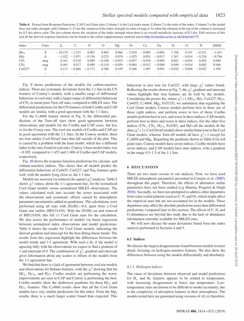
Table 4. Extract from Response Functions. CAP Cool Giant stars. Column 1 is the Lick index name, Column 2 is the units of the index, Column 3 is the modelbase star index strength, and Columns 4–13 are the variation of the index strength (in units of mag or Å) when the element at the top of the column is increasedby 0.3 dex above solar. The last column shows the variation of the index strength when there is an overall metallicity increase of 0.3 dex. Full versions of thisand all the derived response functions can be found in the online supplementary material and at http://uclandata.uclan.ac.uk/id/eprint/175.
Index Units I0 C N O Mg Fe Ca Na Si Cr Ti [M/H]
HδA Å − 10.125 − 2.337 0.007 0.865 0.966 − 2.010 − 0.085 − 0.003 1.768 0.151 − 0.321 −1.433HδF Å − 1.922 − 1.071 − 0.156 0.225 0.074 − 1.025 0.031 − 0.017 1.267 − 0.014 − 0.254 −0.794CN1 mag 0.341 0.510 0.089 − 0.108 − 0.053 − 0.057 − 0.010 − 0.005 0.022 − 0.016 0.002 0.040CN2 mag 0.461 0.517 0.089 − 0.110 − 0.059 − 0.064 − 0.012 − 0.004 0.049 − 0.014 0.002 0.046Ca4227 Å 4.111 − 0.866 − 0.172 0.386 0.439 0.266 1.897 0.091 − 0.010 − 0.040 − 0.023 1.430... ... ... .... ... ... ... ... ... ... ... ... ...
Fig. 9 shows predictions of the models for carbon-sensitiveindices. There are systematic deviations from the 1:1 line in the CNfeatures of Conroy’s models, with a smaller range of differentialbehaviour in cool stars with a larger range of differential behaviourof CN2 in metal-poor Turn-off stars, compared to MILES stars. Thedifferential predictions for the CN features of both Coelho and CAPmodels are similar, with a good agreement with the 1:1 lines.
For the C24668 feature shown in Fig. 9, the differential pre-dictions of the Turn-off stars show good agreement betweenobservations and models for the Coelho and CAP cases, but lessso for the Conoy case. The cool star models of Coelho and CAP arein good agreement with the 1:1 lines. In the Conroy models, thereare four outlier Cool Dwarf stars that fall outside of the plot. Thisis caused by a problem with the base model, which has a differentindex to the ones found in real stars. Conroy’s base model index was−0.105, compared to 1.453 and 1.406 of Coelho and CAP models,respectively.
Fig. 10 shows the response function predictions for calcium- andsodium-sensitive indices. This shows that all models predict thedifferential behaviour of Ca4455, Ca4227, and NaD features quitewell, with the models lying close to, the 1:1 line.
Models are assessed via reduced chi-square (χ2ν ) analysis. Table 5
shows χ2ν values, about the 1:1 agreement line, for the normalized
Cool Giant models versus normalized MILES observations. Thevalues calculated took into account the errors associated withthe observations and systematic offsets caused by atmosphericparameter uncertainties added in quadrature. The calculations wereperformed using all stars with [Fe/H]>-0.4, apart from a CoolGiant star outlier (HD131430). With the [Fe/H] cut and removalof HD131430, this left 11 Cool Giant stars for the calculation.We also assess the performance of models via linear regressionbetween normalized index observations and model predictions.Table 6 shows the results for Cool Giant models, indicating thederived gradient and intercept for the best-fitting linear trends. Theresults from this regression highlight the differences between themodel trends and 1:1 agreement. With such a fit, if the model isagreeing fully with the observations we expect to find a gradient of1 and intercept of 0. The combination of χ2
ν , gradient and interceptgives information about any scatter or offsets of the models fromthe 1:1 agreement line.
We find that there is a lack of agreement between cool star modelsand observations for Balmer features, with the χ2
ν showing that forHδA, Hγ A, and Hγ F Coelho models are performing the worst,improvements are seen in CAP and Conroy is performing the best.Coelho models show the shallowest gradients for these HδA andHγ A features. The C24668 results show that all the Cool Giantmodels have very similar predictions for this index. From the Mgb
results, there is a much larger scatter found than expected. This
behaviour is also true for Ca4227, with large χ2ν values found.
Reflecting the results shown in Fig. 7, the χ2ν , gradient and intercept
values highlight that iron features are fit well by the models.Considering the poorer fits, where χ2
ν >1 (HδA, HδF, Ca4227, Hγ F,Ca4455, C24668, Mgb, Fe5335), we summarize that regarding theCool Giant models, Conroy models perform best in three out ofthose eight indices, and perform worst in two of them; Coelhomodels perform best in two, and worst in three indices; CAP modelsperform best in three and worst in three indices. For the other fiveindices (CN1, CN2, Hγ A, Fe4383, and Hβ) all the models fit thedata (χ2
ν <1). Cool Dwarf models show similar behaviour to the CoolGiant models, whereas Turn-off models all have χ2
ν <1 except forC24668 and Mgb. Regarding the gradients shown in Table 6 for redgiant stars, Conroy models have seven indices, Coelho models haveseven indices, and CAP models have nine indices, with a gradientin the range 0.5–1.5 of the 1:1 line.
6 D ISCUSSION
There are two main caveats to our analysis. First, we have usedMILES atmospheric parameters presented in Cenarro et al. (2007)throughout this paper. Therefore, the effects of alternative stellarparameters have not been studied (e.g Sharma, Prugniel & Singh2016). Secondly, we have not attempted to address other departuresfrom solar-scaled patterns (such as C, N, and O), which might affectthe empirical stars but are not accounted for in the models. Thesedepartures may affect the absolute predictions more than differentialpredictions, compared later in this section. The effects of C, N, andO abundances are beyond this study due to the lack of abundanceinformation currently available for MILES stars.
We will now discuss the main deviations found from the indexanalysis performed in Sections 4 and 5.
6.1 Indices
We discuss the largest disagreements found between models in moredetail, focusing on hydrogen-sensitive features. We also show thedifferences between using the models differentially and absolutely.
6.1.1 Hydrogen indices
The cause of deviations between observed and model predictionsfor Hγ and Hδ features appears to be related to temperature,with increasing disagreement at lower star temperature. Low-temperature stars are known to be difficult to model accurately, dueto the complexity of absorption features in their atmospheres. Themodels tested here are generated using versions of ATLAS therefore,
MNRAS 486, 1814–1832 (2019)
Dow
nloaded from https://academ
ic.oup.com/m
nras/article-abstract/486/2/1814/5381560 by University of C
entral Lancashire user on 30 April 2019
1824 A. T. Knowles et al.
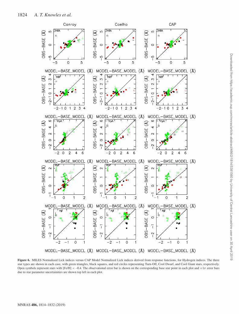
Figure 6. MILES Normalized Lick indices versus CAP Model Normalized Lick indices derived from response functions, for Hydrogen indices. The threestar types are shown in each case, with green triangles, black squares, and red circles representing Turn-Off, Cool Dwarf, and Cool Giant stars, respectively.Open symbols represent stars with [Fe/H] < –0.4. The observational error bar is shown on the corresponding base star point in each plot and +1σ error barsdue to star parameter uncertainities are shown top left in each plot.
MNRAS 486, 1814–1832 (2019)
Dow
nloaded from https://academ
ic.oup.com/m
nras/article-abstract/486/2/1814/5381560 by University of C
entral Lancashire user on 30 April 2019
Stellar spectral models compared with empirical data 1825
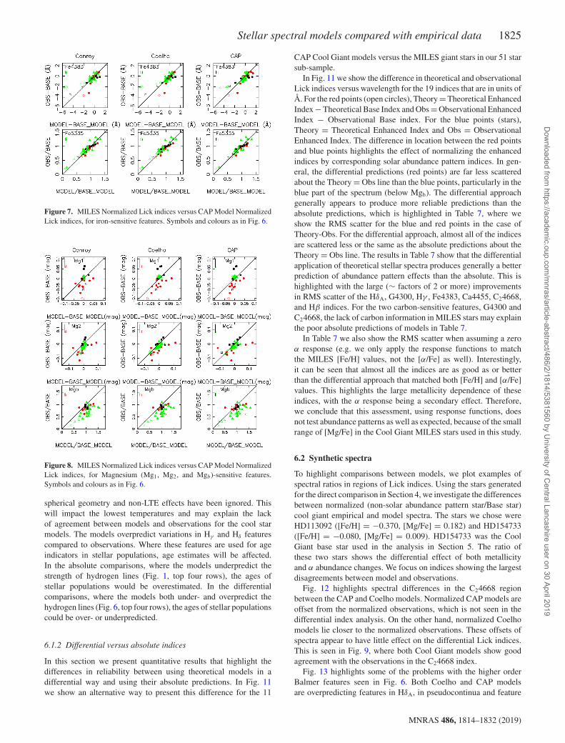
Figure 7. MILES Normalized Lick indices versus CAP Model NormalizedLick indices, for iron-sensitive features. Symbols and colours as in Fig. 6.
Figure 8. MILES Normalized Lick indices versus CAP Model NormalizedLick indices, for Magnesium (Mg1, Mg2, and Mgb)-sensitive features.Symbols and colours as in Fig. 6.
spherical geometry and non-LTE effects have been ignored. Thiswill impact the lowest temperatures and may explain the lackof agreement between models and observations for the cool starmodels. The models overpredict variations in Hγ and Hδ featurescompared to observations. Where these features are used for ageindicators in stellar populations, age estimates will be affected.In the absolute comparisons, where the models underpredict thestrength of hydrogen lines (Fig. 1, top four rows), the ages ofstellar populations would be overestimated. In the differentialcomparisons, where the models both under- and overpredict thehydrogen lines (Fig. 6, top four rows), the ages of stellar populationscould be over- or underpredicted.
6.1.2 Differential versus absolute indices
In this section we present quantitative results that highlight thedifferences in reliability between using theoretical models in adifferential way and using their absolute predictions. In Fig. 11we show an alternative way to present this difference for the 11
CAP Cool Giant models versus the MILES giant stars in our 51 starsub-sample.
In Fig. 11 we show the difference in theoretical and observationalLick indices versus wavelength for the 19 indices that are in units ofÅ. For the red points (open circles), Theory = Theoretical EnhancedIndex − Theoretical Base Index and Obs = Observational EnhancedIndex − Observational Base index. For the blue points (stars),Theory = Theoretical Enhanced Index and Obs = ObservationalEnhanced Index. The difference in location between the red pointsand blue points highlights the effect of normalizing the enhancedindices by corresponding solar abundance pattern indices. In gen-eral, the differential predictions (red points) are far less scatteredabout the Theory = Obs line than the blue points, particularly in theblue part of the spectrum (below Mgb). The differential approachgenerally appears to produce more reliable predictions than theabsolute predictions, which is highlighted in Table 7, where weshow the RMS scatter for the blue and red points in the case ofTheory-Obs. For the differential approach, almost all of the indicesare scattered less or the same as the absolute predictions about theTheory = Obs line. The results in Table 7 show that the differentialapplication of theoretical stellar spectra produces generally a betterprediction of abundance pattern effects than the absolute. This ishighlighted with the large (∼ factors of 2 or more) improvementsin RMS scatter of the HδA, G4300, Hγ , Fe4383, Ca4455, C24668,and Hβ indices. For the two carbon-sensitive features, G4300 andC24668, the lack of carbon information in MILES stars may explainthe poor absolute predictions of models in Table 7.
In Table 7 we also show the RMS scatter when assuming a zeroα response (e.g. we only apply the response functions to matchthe MILES [Fe/H] values, not the [α/Fe] as well). Interestingly,it can be seen that almost all the indices are as good as or betterthan the differential approach that matched both [Fe/H] and [α/Fe]values. This highlights the large metallicity dependence of theseindices, with the α response being a secondary effect. Therefore,we conclude that this assessment, using response functions, doesnot test abundance patterns as well as expected, because of the smallrange of [Mg/Fe] in the Cool Giant MILES stars used in this study.
6.2 Synthetic spectra
To highlight comparisons between models, we plot examples ofspectral ratios in regions of Lick indices. Using the stars generatedfor the direct comparison in Section 4, we investigate the differencesbetween normalized (non-solar abundance pattern star/Base star)cool giant empirical and model spectra. The stars we chose wereHD113092 ([Fe/H] = −0.370, [Mg/Fe] = 0.182) and HD154733([Fe/H] = −0.080, [Mg/Fe] = 0.009). HD154733 was the CoolGiant base star used in the analysis in Section 5. The ratio ofthese two stars shows the differential effect of both metallicityand α abundance changes. We focus on indices showing the largestdisagreements between model and observations.
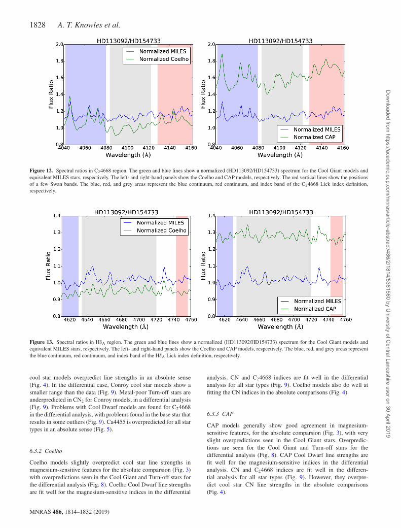
Fig. 12 highlights spectral differences in the C24668 regionbetween the CAP and Coelho models. Normalized CAP models areoffset from the normalized observations, which is not seen in thedifferential index analysis. On the other hand, normalized Coelhomodels lie closer to the normalized observations. These offsets ofspectra appear to have little effect on the differential Lick indices.This is seen in Fig. 9, where both Cool Giant models show goodagreement with the observations in the C24668 index.
Fig. 13 highlights some of the problems with the higher orderBalmer features seen in Fig. 6. Both Coelho and CAP modelsare overpredicting features in HδA, in pseudocontinua and feature
MNRAS 486, 1814–1832 (2019)
Dow
nloaded from https://academ
ic.oup.com/m
nras/article-abstract/486/2/1814/5381560 by University of C
entral Lancashire user on 30 April 2019
1826 A. T. Knowles et al.
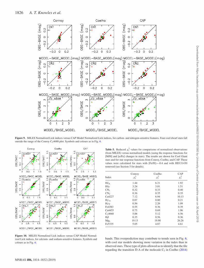
Figure 9. MILES Normalized Lick indices versus CAP Model Normalized Lick indices, for carbon- and nitrogen-sensitive features. Four cool dwarf stars falloutside the range of the Conroy C24688 plot. Symbols and colours as in Fig. 6.
Figure 10. MILES Normalized Lick indices versus CAP Model Normal-ized Lick indices, for calcium- and sodium-sensitive features. Symbols andcolours as in Fig. 6.
Table 5. Reduced χ2ν values for comparisons of normalized observations
(from MILES) versus normalized models (using the response functions for[M/H] and [α/Fe] changes in stars). The results are shown for Cool Giantstars and for star response functions from Conroy, Coelho, and CAP. Thesevalues were calculated for stars with [Fe/H]>–0.4 and with HD131430removed (see Section 5 for details).
Conroy Coelho CAPIndex χ2
ν χ2ν χ2
ν
HδA 1.44 6.21 1.92HδF 3.24 3.01 1.51CN1 0.32 0.33 0.40CN2 0.36 0.35 0.35Ca4227 7.12 6.94 10.13Hγ A 0.07 0.80 0.21Hγ F 0.56 2.26 1.09Fe4383 0.55 0.36 0.39Ca4455 0.75 0.69 1.06C24668 5.06 5.12 4.56Hβ 0.35 0.56 0.36Mgb 19.13 19.90 26.26Fe5335 5.05 4.87 4.61
bands. This overprediction may contribute to trends seen in Fig. 6,with cool star models showing more variation in the index than inobserved stars. These type of plots allowed us to identify that the fileregarding the transition D-A of the molecule C2 in Coelho (2014)
MNRAS 486, 1814–1832 (2019)
Dow
nloaded from https://academ
ic.oup.com/m
nras/article-abstract/486/2/1814/5381560 by University of C
entral Lancashire user on 30 April 2019

Stellar spectral models compared with empirical data 1827
Table 6. Gradient and intercept values calculated from a linear regression for comparisons of normalized observations (from MILES) versus normalizedmodels (using the response functions for [M/H] and [α/Fe] changes in stars). The results are shown for Cool Giant stars and for star response functions fromConroy, Coelho, and CAP. These values were calculated for stars with [Fe/H]>−0.4 and with HD131430 removed.
Conroy Coelho CAP
Index Gradient Intercept Gradient Intercept Gradient Intercept
HδA 0.55 ± 0.12 0.19 ± 0.18 Å 0.32 ± 0.07 0.19 ± 0.18 Å 0.50 ± 0.12 0.20 ± 0.20 ÅHδF 0.25 ± 0.06 − 0.01 ± 0.06 Å 0.25 ± 0.06 − 0.01 ± 0.07 Å 0.33 ± 0.08 0.00 ± 0.07 ÅCN1 2.33 ± 0.37 0.00 ± 0.01 mag 1.02 ± 0.31 − 0.01 ± 0.01 mag 0.83 ± 0.28 0.00 ± 0.02 magCN2 2.84 ± 0.40 0.00 ± 0.01 mag 0.84 ± 0.26 − 0.01 ± 0.01 mag 0.83 ± 0.26 0.00 ± 0.01 magCa4227 0.19 ± 0.30 0.68 ± 0.30 0.17 ± 0.32 0.70 ± 0.33 0.03 ± 0.24 0.84 ± 0.25Hγ A 1.03 ± 0.20 − 0.07 ± 0.09 Å 0.35 ± 0.05 − 0.01 ± 0.08 Å 0.54 ± 0.09 − 0.06 ± 0.08 ÅHγ F 0.82 ± 0.22 0.02 ± 0.06 Å 0.39 ± 0.12 0.03 ± 0.06 Å 0.53 ± 0.15 0.03 ± 0.06 ÅFe4383 1.85 ± 0.29 − 0.32 ± 0.15 Å 0.84 ± 0.13 − 0.31 ± 0.15 Å 1.39 ± 0.20 − 0.33 ± 0.14 ÅCa4455 0.94 ± 0.29 0.07 ± 0.29 1.07 ± 0.31 − 0.10 ± 0.31 0.92 ± 0.42 0.10 ± 0.42C24668 1.05 ± 0.16 0.01 ± 0.17 0.85 ± 0.13 0.20 ± 0.13 0.80 ± 0.09 0.26 ± 0.10Hβ 1.73 ± 0.76 0.13 ± 0.06 Å − 2.87 ± 1.14 0.13 ± 0.06 Å 2.13 ± 0.86 0.14 ± 0.06 ÅMgb 0.63 ± 0.20 0.23 ± 0.20 0.60 ± 0.24 0.27 ± 0.24 0.39 ± 0.19 0.47 ± 0.19Fe5335 0.87 ± 0.15 0.07 ± 0.15 0.91 ± 0.15 0.04 ± 0.16 0.95 ± 0.15 0.00 ± 0.15
Figure 11. Comparison between the differential and absolute predictionsof line strengths for the 19 indices, with units of Å, as a function ofwavelength. This is illustrated for the CAP Cool Giant models, with thesame parameter cuts as Table 5, leaving 11 stars. The vertical axis showsdifferences between theoretical and observed index values. Red and bluepoints represent the differential and absolute application of the models,respectively. The absolute models have been produced with parameters thatmatch those of Cenarro et al. (2007) MILES parameters.
models was corrupted. This corruption does not affect any of thiswork, but is discussed and illustrated in Appendix A.
6.3 Model strengths and weaknesses
Comparisons between models were discussed in Sections 4 and 5.Here, we summarize the main strengths and weaknesses of eachindividual model compared to observations, in terms of absoluteand differential behaviours.
We find that all three models do not fit the Balmer features well, inan absolute and differential analysis, with the greatest problems seenin cool stars models in an absolute sense (Fig. 1) and in all star-typesin a differential sense (Fig. 6). All three models do quite well at pre-dicting iron-sensitive features (Figs 2 and 7). All models tend to un-derpredict C24668 line strengths in an absolute comparsion (Fig. 4).Calcium- and sodium (Figs 5 and 10)-sensitive features also show
Table 7. RMS scatter about the Theory = Obs line of the three differentapplications of CAP Cool Giant model predictions. The columns representthe index name, the differential predictions, absolute predictions, anddifferential predictions fixing the α response to zero, respectively. In generalthe differential scatter is smaller or performing the same as the absolutebehaviour.
Index Absolute Differential DifferentialÅ Å (α-fixed) Å
HδA 2.86 1.02 0.59HδF 0.75 0.60 0.36Ca4227 1.14 1.23 1.10G4300 2.39 0.86 0.51Hγ A 2.54 0.49 0.51Hγ F 1.00 0.26 0.23Fe4383 1.13 0.56 0.73Ca4455 0.69 0.22 0.18Fe4531 0.53 0.28 0.29C24668 4.03 1.00 1.01Hβ 0.74 0.22 0.22Fe5015 0.53 0.30 0.27Mgb 0.77 1.03 0.86Fe5270 1.08 1.02 1.07Fe5335 0.69 0.38 0.43Fe5406 0.36 0.36 0.34Fe5709 0.50 0.54 0.54Fe5782 0.34 0.27 0.24NaD 0.59 0.73 0.72
fairly good agreement with the data, with no clear systematics inboth an absolute and differential sense, other than those noted below.
6.3.1 Conroy
Recall that in the absolute comparsions (Section 4), Conroy modelswere produced via interpolation in a pre-existing grid. Some sys-tematic offsets between Conroy models and observations are seen inthe absolute comparisons of magnesium-sensitive features, with thecool star models overpredicting feature strengths (Fig. 3). ConroyCool Giant and Turn-off models tend to overpredict magnesium-sensitive line strengths but show a good fit for Cool Dwarf stars, inthe differential analysis (Fig. 8). For CN1 and CN2 indices, Conroy
MNRAS 486, 1814–1832 (2019)
Dow
nloaded from https://academ
ic.oup.com/m
nras/article-abstract/486/2/1814/5381560 by University of C
entral Lancashire user on 30 April 2019
1828 A. T. Knowles et al.
Figure 12. Spectral ratios in C24668 region. The green and blue lines show a normalized (HD113092/HD154733) spectrum for the Cool Giant models andequivalent MILES stars, respectively. The left- and right-hand panels show the Coelho and CAP models, respectively. The red vertical lines show the positionsof a few Swan bands. The blue, red, and grey areas represent the blue continuum, red continuum, and index band of the C24668 Lick index definition,respectively.
Figure 13. Spectral ratios in HδA region. The green and blue lines show a normalized (HD113092/HD154733) spectrum for the Cool Giant models andequivalent MILES stars, respectively. The left- and right-hand panels show the Coelho and CAP models, respectively. The blue, red, and grey areas representthe blue continuum, red continuum, and index band of the HδA Lick index definition, respectively.
cool star models overpredict line strengths in an absolute sense(Fig. 4). In the differential case, Conroy cool star models show asmaller range than the data (Fig. 9). Metal-poor Turn-off stars areunderpredicted in CN2 for Conroy models, in a differential analysis(Fig. 9). Problems with Cool Dwarf models are found for C24668in the differential analysis, with problems found in the base star thatresults in some outliers (Fig. 9). Ca4455 is overpredicted for all startypes in an absolute sense (Fig. 5).
6.3.2 Coelho
Coelho models slightly overpredict cool star line strengths inmagnesium-sensitive features for the absolute comparsion (Fig. 3)with overpredictions seen in the Cool Giant and Turn-off stars forthe differential analysis (Fig. 8). Coelho Cool Dwarf line strengthsare fit well for the magnesium-sensitive indices in the differential
analysis. CN and C24668 indices are fit well in the differentialanalysis for all star types (Fig. 9). Coelho models also do well atfitting the CN indices in the absolute comparisons (Fig. 4).
6.3.3 CAP
CAP models generally show good agreement in magnesium-sensitive features, for the absolute comparsion (Fig. 3), with veryslight overpredictions seen in the Cool Giant stars. Overpredic-tions are seen for the Cool Giant and Turn-off stars for thedifferential analysis (Fig. 8). CAP Cool Dwarf line strengths arefit well for the magnesium-sensitive indices in the differentialanalysis. CN and C24668 indices are fit well in the differen-tial analysis for all star types (Fig. 9). However, they overpre-dict cool star CN line strengths in the absolute comparisons(Fig. 4).
MNRAS 486, 1814–1832 (2019)
Dow
nloaded from https://academ
ic.oup.com/m
nras/article-abstract/486/2/1814/5381560 by University of C
entral Lancashire user on 30 April 2019
Stellar spectral models compared with empirical data 1829
7 C O N C L U S I O N S
In this study, we have tested both the differential and absoluteline-strength predictions of three state-of-the-art theoretical stellarmodel libraries, using empirical MILES stellar spectra. First, wedirectly tested three stellar model libraries, matching the parametersof Teff, log g, [Fe/H], and [α/Fe] of MILES stars to study trendsand aid the differential tests. We then used response functions toaccount for changes in [Fe/H] and [α/Fe] abundances. The latestresponse functions calculated here are made publicly available insupplementary data online.
In summary, we find that:
(i) Differences between models are generally less significant thanthe ways in which models vary from the data.
(ii) All three models libraries do well at predicting abundancepattern effects in certain features, particularly those sensitive toiron and sodium.
(iii) Problems exist in the Balmer features of all models, withoverprediction of the variation in Hδ and Hγ indices present in coolstar models. There is no clear abudance pattern correlations shownin Hβ, however there is a weak abundance effect with Hβ0 (seeAppendix B).
(iv) Using diagnostic index and spectral plots (like those shownin Figs 9 and 12), we identified a corrupted file of the transitionD-A of C2, describing the Swan bands in Coelho (2014) models.This corrupted file was corrected for this work. Appendix A (FigsA1 and A2) shows the effects of that corruption and its correction.
(v) As expected, the absolute differences between models and ob-servations are generally worse than using the differential behaviour.This was investigated using the CAP Cool Giant models. In theapplication of these models, the differential approach produces lessor similar scatter about the agreements with observations than theabsolute predictions. In particular, the differential predictions ofsome hydrogen features are scattered by a factor of ∼2 less than theabsolute predictions. A large reduction in scatter between the twoapproaches is also seen in G4300 and C24668 indices.
(vi) In general, the largest differences between the observationsand absolute model predictions are seen at lower temperatures,which may be explained by the omission of non-LTE and 3Dgeometry effects in all the models. The features that are largelyaffected in this temperature regime are the higher order Balmerfeatures, with models overpredicting variations of line-strengthindex with abundance pattern in both differential and absolutepredictons.
This work highlights the benefits of a differential approach tomodelling abundance patterns. However, it still has its limitationsand errors that we have attempted to show in this paper. Twocaveats of this analysis have been highlighted in Section 6. Wehave not investigated if different stellar parameters for the MILESstars would affect our conclusions. We have also not attemptedto study any abundances differences other than [α/Fe], such asC, N, and O, which might affect the empirical stars but are notchanged from scaled solar in the models. If more abundances aremeasured for MILES stars, these effects can be studied in future.However, it can be seen that different models produce slightlydifferent predictions of abundance pattern effects, and awareness ofthis will be important in the application of these models. We haveshown that using the models’ differential predictions of abundancepattern effects produces a better agreement with observations thanusing the absolute predictions, particularly at bluer wavelengths.This finding will be used in the generation of a new semi-empirical
model library of stars that will make use of both observed spectraand differential predictions of theoretical spectra.
AC K N OW L E D G E M E N T S
The authors would like to thank the STFC for providing ATK withthe studentship for his PhD studies as well as the IAC for providingthe support and funds that allowed ATK to visit the instituteon two occasions. AES acknowledges travel support from grantAYA2016-77237-C3-1-P from the Spanish Ministry of Economyand Competitiveness (MINECO). PYTHON code used for blurringspectra was written by Jesus Falcon-Barroso. The authors wouldlike to thank S. Earp and the anonymous referee, whose commentsand suggestions improved the quality of this manuscript.
REFERENCES
Allende Prieto C. et al., 2014, A&A, 568, A7Allende Prieto C., Koesterke L., Hubeny I., Bautista M. A., Barklem P. S.,
Nahar S. N., 2018, A&A, 618, A25Asplund M., Grevesse N., Sauval A. J., 2005, in Barnes T. G., III, Bash F. N.,
eds, ASP Conf. Ser. Vol. 336, Cosmic Abundances as Records of StellarEvolution and Nucleosynthesis. Astron. Soc. Pac., San Francisco, p. 25
Asplund M., Grevesse N., Sauval A. J., Scott P., 2009, ARA&A, 47, 481Bell R. A., Paltoglou G., Tripicco M. J., 1994, MNRAS, 268, 771Bembenek Z., Kepa R., Rytel M., 1997, JMS, 183, 1Bertone E., Buzzoni A., Chavez M., Rodrıguez-Merino L. H., 2008, A&A,
485, 823Brooke J. S. A., Bernath P. F., Schmidt T. W., Bacskay G. B., 2013, J. Quant.
Spec. Radiat. Transf., 124, 11Brooke J. S. A., Ram R. S., Western C. M., Li G., Schwenke D. W., Bernath
P. F., 2014, ApJS, 210, 23Castelli F., 2005a, Mem. Soc. Astron. Ital. Suppl., 8, 25Castelli F., 2005b, Mem. Soc. Astron. Ital. Suppl., 8, 34Cenarro A. J. et al., 2007, MNRAS, 374, 664Cervantes J. L., Vazdekis A., 2009, MNRAS, 392, 691Coelho P., Barbuy B., Melendez J., Schiavon R. P., Castilho B. V., 2005,
A&A, 443, 735Coelho P., Bruzual G., Charlot S., Weiss A., Barbuy B., Ferguson J. W.,
2007, MNRAS, 382, 498Coelho P. R. T., 2014, MNRAS, 440, 1027Colin R., Bernath P. F., 2010, JMS, 263, 120Conroy C., van Dokkum P., 2012, ApJ, 747, 69Conroy C., Graves G. J., van Dokkum P. G., 2014, ApJ, 780, 33da Silva R., Milone A. C., Reddy B. E., 2011, A&A, 526, A71Delgado Mena E., Israelian G., Gonzalez Hernandez J. I., Bond J. C., Santos
N. C., Udry S., Mayor M., 2010, ApJ, 725, 2349Falcon-Barroso J., Sanchez-Blazquez P., Vazdekis A., Ricciardelli E.,
Cardiel N., Cenarro A. J., Gorgas J., Peletier R. F., 2011, A&A, 532,A95
Gonneau A. et al., 2016, A&A, 589, A36Grevesse N., Sauval A. J., 1998, Space Sci. Rev., 85, 161Gustafsson B., Edvardsson B., Eriksson K., Jørgensen U. G., Nordlund Å.,
Plez B., 2008, A&A, 486, 951Holtzman J. A. et al., 2015, AJ, 150, 148Johnson C. I., Rich R. M., Kobayashi C., Kunder A., Koch A., 2014, AJ,
148, 67Kepa R., Para A., Rytel M., Zachwieja M., 1996, JMS, 178, 189Koesterke L., 2009, in Hubeny I., Stone J. M., MacGregor K., Werner K.,
eds, AIP Conf. Ser. Vol. 1171, Am. Inst. Phys., New York, QuantitativeSpectroscopy in 3D, p. 73
Korn A. J., Maraston C., Thomas D., 2005, A&A, 438, 685Kurucz R., 1993, ATLAS9 Stellar Atmosphere Programs and 2 km/s grid.
Kurucz CD-ROM No. 13, Smithsonian Astrophysical Observatory,Cambridge, MA
Kurucz R. L., 1979, ApJS, 40, 1
MNRAS 486, 1814–1832 (2019)
Dow
nloaded from https://academ
ic.oup.com/m
nras/article-abstract/486/2/1814/5381560 by University of C
entral Lancashire user on 30 April 2019

1830 A. T. Knowles et al.
Kurucz R. L., 1996, in Strassmeier K. G., Linsky J. L., eds, Proc. IAUSymp. Vol. 176, Stellar Surface Structure, Kluwer Academic Publishers,Dordrecht, p. 523
Kurucz R. L., 2005, Mem. Soc. Astron. Ital. Suppl., 8, 14Kurucz R. L., , Avrett E. H., 1981, SAO Spec. Rep., 391, 1Lee H.-c., et al., 2009, ApJ, 694, 902Letarte B., Hill V., Tolstoy E., 2007, in Emsellem E., Wozniak H., Massacrier
G., Gonzalez J.-F., Devriendt J., Champavert N., eds, EAS Publ. Ser.Vol. 24, EAS Publications Series, EDP Sciences, Le Ulis, France,p. 33
Mannucci F., 2008, Chin. J. Astron. Astrophys. Suppl., 8, 143Maoz D., Sharon K., Gal-Yam A., 2010, ApJ, 722, 1879Martins L. P., Coelho P., 2007, MNRAS, 381, 1329Meszaros S. et al., 2012, AJ, 144, 120Milone A. D. C., Sansom A. E., Sanchez-Blazquez P., 2011, MNRAS, 414,
1227Munari U., Sordo R., Castelli F., Zwitter T., 2005, A&A, 442, 1127Onodera M. et al., 2015, ApJ, 808, 161Pagel B. E. J., 2009, Nucleosynthesis and Chemical Evolution of Galaxies,
Cambridge University Press, CambridgePercival S. M., Salaris M., Cassisi S., Pietrinferni A., 2009, ApJ, 690, 427Poggianti B. M., Barbaro G., 1997, A&A, 325, 1025Proctor R. N., Sansom A. E., 2002, MNRAS, 333, 517Prugniel P., Koleva M., Ocvirk P., Le Borgne D., Soubiran C., 2007, in
Vazdekis A., Peletier R., eds, Proc. IAU Symp. 241, Stellar Popula-tions as Building Blocks of Galaxies, Kluwer Academic Publishers,Dordrecht, p. 68
Rose J. A., 1984, AJ, 89, 1238Sanchez-Blazquez P. et al., 2006, MNRAS, 371, 703Sansom A. E., Milone A. d. C., Vazdekis A., Sanchez-Blazquez P., 2013,
MNRAS, 435, 952Sbordone L., Bonifacio P., Castelli F., Kurucz R. L., 2004, Mem. Societa
Astron. Ital. Suppl., 5, 93Schiavon R. P., 2007, ApJS, 171, 146Sesto L. A., Faifer F. R., Smith Castelli A. V., Forte J. C., Escudero C. G.,
2018, MNRAS, 479, 478Sharma K., Prugniel P., Singh H. P., 2016, A&A, 585, A64Sullivan M. et al., 2006, ApJ, 648, 868Swan W., 1875, Trans. R. Soc. Edinburugh, 21, 411Thomas D., Maraston C., Bender R., 2003, MNRAS, 339, 897Thomas D., Maraston C., Bender R., Mendes de Oliveira C., 2005, ApJ,
621, 673Thomas D., Johansson J., Maraston C., 2011, MNRAS, 412, 2199Trager S. C., Faber S. M., Worthey G., Gonzalez J. J., 2000, AJ, 119, 1645Tripicco M. J., Bell R. A., 1995, AJ, 110, 3035Vazdekis A. et al., 2015, MNRAS, 449, 1177Vazdekis A., 2011, LECTOR: Line-strengths in One-dimensional ASCII
Spectra, Astrophysics Source Code Library, record ascl:1104.006Vazdekis A., Sanchez-Blazquez P., Falcon-Barroso J., Cenarro A. J., Beasley
M. A., Cardiel N., Gorgas J., Peletier R. F., 2010, MNRAS, 404,1639
Villaume A., Brodie J., Conroy C., Romanowsky A. J., van Dokkum P.,2017, ApJ, 850, L14
Walcher C. J., Coelho P., Gallazzi A., Charlot S., 2009, MNRAS, 398, L44Worthey G., 1994, ApJS, 95, 107Worthey G., Ottaviani D. L., 1997, ApJS, 111, 377Worthey G., Faber S. M., Gonzalez J. J., 1992, ApJ, 398, 69Zachwieja M., 1995, J. Mol. Spectrosc., 170, 285Zachwieja M., 1997, J. Mol. Spectrosc., 182, 18
SUPPORTI NG INFORMATI ON
Supplementary data are available at MNRAS online.
Please note: Oxford University Press is not responsible for thecontent or functionality of any supporting materials supplied bythe authors. Any queries (other than missing material) should bedirected to the corresponding author for the article.
APPENDI X A : C OELHO LATEST R EVI SIO NS
During the work for this paper, we identified a problem in theC24668 region in the Coelho models. The origin of this problem wasfound to be in the C2 line list of these models. Specifically there wasa corruption with the file containing the D-A transition. This is thelikely origin of the missing opacity, which can be seen around 4000Å in the second panel in fig. 10 of Coelho (2014). This corruptionled to the problems shown in Figs A1 and A2. It can be seen in theleft-hand panel of Fig. A1 that there was an issue regarding a lackof variation in the normalized C24668 index for the corrupted (old)Coelho cool star models. This is clarified in the left-hand panel ofFig. A2, which shows that the corrupted Coelho models had almostno variation in the C24668 spectral region with an increase of 0.3dex in carbon. The models were recomputed with a corrected C2
D-A transition for this work and we plot the corrected models inthe right-hand panel of Fig. A1 and in both panels of Fig. A2 (greenlines). It can be seen in the right-hand panel of Fig. A1 that thecorruption is ammended and the models now lie in closer agreementwith MILES observations. This improvement is reflected in thespectral plots in Fig. A2, with Coelho’s new models showing strongabsorption features of the Swan bands (Swan 1875; Gonneau et al.2016). Typical features, orginating from the (1,0) vibrational plusrotational transitions, in the Swan bands exist at 4684, 4697, 4715,and 4737 Å and these locations are shown in Fig. A2. Numerically,this correction results in an increase in C24668 carbon responsefrom 0.014 to 10.266 Å and an increase in C24668 overall metalresponse from −0.042 to 1.552 Å between the old and correctedCoelho models, respectively. The response functions presented inthe online data incorporate these corrections for Coelho’s mod-els. These corrections will be present in future works involvingCoelho models. This correction has negligible effect on the otherindices.
MNRAS 486, 1814–1832 (2019)
Dow
nloaded from https://academ
ic.oup.com/m
nras/article-abstract/486/2/1814/5381560 by University of C
entral Lancashire user on 30 April 2019

Stellar spectral models compared with empirical data 1831
Figure A1. MILES Normalized Lick indices versus the Coelho (2014) models initially found in this study (Coelho Old) and the revised Coelho (Coelho New)models for C24668. Symbols and colours as in Fig. 6.
Figure A2. Spectral ratios in the C24668 region. The left-hand plot shows a comparison between normalized spectra (C+0.3/Solar) for the Coelho old andrevised Cool Giant models. The right-hand plot shows a comparsion between normalized spectra (Z + 0.3 Solar) for the Coelho old and revised Cool Giantmodels. In both plots the red vertical lines show positions of a few Swan Band (1,0) features and the blue, red, and grey areas represent the blue continuum,red continuum, and index band of the C24668 Lick index definition, respectively.
MNRAS 486, 1814–1832 (2019)
Dow
nloaded from https://academ
ic.oup.com/m
nras/article-abstract/486/2/1814/5381560 by University of C
entral Lancashire user on 30 April 2019
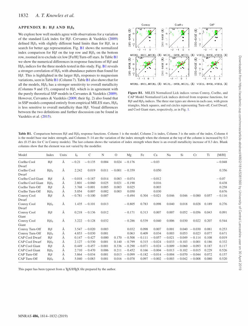
1832 A. T. Knowles et al.
APPENDIX B: Hβ A N D Hβ0
We explore how well models agree with observations for a variationof the standard Lick index for Hβ. Cervantes & Vazdekis (2009)defined Hβ0 with slightly different band limits than for Hβ, in asearch for better age representation. Fig. B1 shows the normalizedindex comparison for Hβ on the top row and Hβ0 on the bottomrow, zoomed in to exclude six low [Fe/H] Turn-off stars. In Table B1we show the numerical differences in response functions of Hβ andHβ0 indices for the three models tested in this study. Fig. B1 revealsa stronger correlation of Hβ0 with abundance pattern than found forHβ. This is highlighted in the larger Hβ0 responses to magnesiumvariations, seen in Table B1 (Column 7). Table B1 also shows that forall the models, Hβ0 has a stronger sensitivity to overall metallicity(Columns 9 and 15), compared to Hβ, which is in agreement withthe purely theoretical SSP models in Cervantes & Vazdekis (2009).However, Cervantes & Vazdekis (2009; their fig. 2) also found thatin SSP models computed entirely from empirical MILES stars, Hβ0
is less sensitive to overall metallicity than Hβ. Visual differencesbetween the two definitions and further discussion can be found inVazdekis et al. (2015).
Figure B1. MILES Normalized Lick indices versus Conroy, Coelho, andCAP Model Normalized Lick indices derived from response functions, forHβ and Hβ0 indices. The three star types are shown in each case, with greentriangles, black squares, and red circles representing Turn-off, Cool Dwarf,and Cool Giant stars, respectively, as in Fig. 1.
Table B1. Comparison between Hβ and Hβ0 response functions. Column 1 is the model, Column 2 is index, Column 3 is the units of the index, Column 4is the model base star index strength, and Columns 5–14 are the variation of the index strength when the element at the top of the column is increased by 0.3dex (0.15 dex for C in Conroy models). The last column shows the variation of index strength when there is an overall metallicity increase of 0.3 dex. Blankcolumns show that the element was not varied by the modeller.
Model Index Units I0 C N O Mg Fe Ca Na Si Cr Ti [M/H]
Coelho CoolDwarf
Hβ Å − 0.21 − 0.135 0.004 0.024 − 0.176 − 0.03 − 0.048
Coelho CoolDwarf
Hβ0 Å 2.242 0.019 0.011 − 0.001 − 0.359 0.050 0.356
Coelho Cool Giant Hβ Å − 0.018 − 0.187 0.014 0.083 − 0.074 − 0.012 − 0.07Coelho Cool Giant Hβ0 Å 2.801 − 0.060 0.025 0.021 − 0.190 0.016 0.438Coelho Turn-Off Hβ Å 3.768 − 0.001 0.005 0.003 0.025 0.003 0.258Coelho Turn-Off Hβ0 Å 5.054 0.007 0.002 0.003 0.050 0.030 0.676Conroy CoolDwarf
Hβ Å − 0.781 − 0.100 0.007 − 0.494 0.304 − 0.021 0.046 0.046 − 0.080 0.057 − 0.116
Conroy CoolDwarf
Hβ0 Å 1.435 − 0.101 0.013 − 0.805 0.783 0.098 0.040 0.018 0.028 0.189 0.276
Conroy CoolGiant
Hβ Å 0.218 − 0.136 0.012 − 0.171 0.313 0.007 0.007 0.052 − 0.056 0.043 0.091
Conroy CoolGiant
Hβ0 Å 3.222 − 0.128 0.032 − 0.286 0.539 0.040 0.006 0.030 0.022 0.207 0.544
Conroy Turn-Off Hβ Å 3.547 − 0.020 0.003 0.032 0.098 0.007 0.001 0.040 − 0.030 0.081 0.253Conroy Turn-Off Hβ0 Å 4.853 − 0.030 0.001 0.063 0.409 0.034 0.003 0.053 0.023 0.077 0.671CAP Cool Dwarf Hβ Å 0.147 − 0.427 0.000 0.170 − 0.508 − 0.111 − 0.057 − 0.021 − 0.049 − 0.114 0.108 0.019CAP Cool Dwarf Hβ0 Å 2.127 − 0.530 0.001 0.140 − 0.799 0.315 − 0.024 − 0.033 − 0.103 − 0.001 0.186 0.332CAP Cool Giant Hβ Å 0.449 − 0.457 − 0.001 0.336 − 0.290 − 0.071 − 0.024 − 0.009 − 0.060 − 0.093 0.187 0.117CAP Cool Giant Hβ0 Å 2.710 − 0.470 0.006 0.211 − 0.452 0.166 − 0.004 − 0.013 − 0.102 − 0.015 0.229 0.526CAP Turn-Off Hβ Å 3.864 − 0.034 0.001 0.013 − 0.099 − 0.182 − 0.014 − 0.004 − 0.070 − 0.044 0.072 0.157CAP Turn-Off Hβ0 Å 5.040 − 0.083 0.001 0.016 − 0.078 0.097 − 0.002 − 0.003 − 0.042 − 0.008 0.080 0.520
This paper has been typeset from a TEX/LATEX file prepared by the author.
MNRAS 486, 1814–1832 (2019)
Dow
nloaded from https://academ
ic.oup.com/m
nras/article-abstract/486/2/1814/5381560 by University of C
entral Lancashire user on 30 April 2019