steering actuator sizing of prototype electric...
TRANSCRIPT
Steering actuator sizing of prototype
electric one-seater Master’s Thesis
GREGOR WERUM
Department of Applied Mechanics
Division of Vehicle Engineering and Autonomous Systems
Vehicle Dynamics Research Group
CHALMERS UNIVERSITY OF TECHNOLOGY
Göteborg, Sweden 2013
Master’s thesis 2013:45

MASTER’S THESIS
Steering actuator sizing of prototype
electric one-seater
GREGOR WERUM
Department of Applied Mechanics
Division of Vehicle Engineering and Autonomous Systems
Vehicle Dynamics Research Group
CHALMERS UNIVERSITY OF TECHNOLOGY
Göteborg, Sweden 2013


Steering actuator sizing of prototype electric one-seater
GREGOR WERUM
© GREGOR WERUM 2013
Master’s Thesis 2013:45
ISSN 1652-8557
Department of Applied Mechanics
Division of Vehicle Engineering and Autonomous Systems
Vehicle Dynamics Research Group
Chalmers University of Technology
SE-412 96 Göteborg
Sweden
Telephone: + 46 (0)31-772 1000
Commissioned by: Volvo Group Advanced Technology & Research
Department of Mechatronics and Software, BF40760
CTP, Volvo Group Trucks Technology
SE-412 88 Göteborg
Sweden
Cover:
CAD drawing of EDV proposed on June 2013
Chalmers Reproservice / Department of Applied Mechanics
Göteborg, Sweden 2013


I
Steering actuator sizing of prototype electric one-seater
Master’s Thesis
GREGOR WERUM
Department of Applied Mechanics
Division of Vehicle Engineering and Autonomous Systems
Vehicle Dynamics Research Group
Chalmers University of Technology
ABSTRACT
This work describes the setting of power requirements of the steering actuator for an
electric demonstration vehicle (EDV). The EDV is a small one-seater vehicle with
mass of approximately ~ 400 kg and is equipped with a steer-by-wire system. The
dimensioning of steering systems components other than the steering actuator is not
discussed in this report.
An analytic method has been developed to estimate maximum expected steering
torque in creep and high speed scenarios. Furthermore, the model allows the
prediction of suspension geometry influence on steering torque amplitude.
The steering effort is analyzed by means of maximum expected tire forces, which are
estimated by a simple physical tire model. In the tire model maximum tire-to-ground
friction is estimated for various driving scenarios considering the physical limits of
the tires. This approach allows the analysis to be performed independent of vehicle
motion and without a detailed dynamic car model.
The general design of the steer-by-wire system and a steering control setup is
presented in order to evaluate the proposed steering system with respect to control
time and precision. This is accomplished for a given actuator setup.
As major outcome of this work the overall power requirements - such as torque,
speed, power and energy demand - of the steering actuator are presented. The rough
actuator requirements have been identified with , and for a linear actuator placed on the steering rack.
This is equivalent to , and
for a rotary actor with steering ratio .
Key words: Steering actuator, Steer-by-wire, Tire model, Suspension geometry
model, Steering control
II
Dimensionering av styraktuator för elektriskt prototypfordon
Examensarbete
GREGOR WERUM
Institutionen för tillämpad mekanik
Avdelningen för fordonsteknik och autonoma system
Forskargruppen fordonsdynamik
Chalmers tekniska högskola
CHALMERS, Applied Mechanics, Master’s Thesis 2013:45 III
Contents
ABSTRACT I
CONTENTS III
PREFACE V
NOTATIONS VI
1 INTRODUCTION 2
1.1 Background 2
1.2 Report contributions 2
1.3 Vehicle parameters 2
1.4 Scope 3
1.5 Structure of report 3
1.6 Coordinate systems 4
2 STEERING SYSTEM DESIGN 6
2.1 Steer-by-wire setup 6
2.2 Suspension model 8
2.3 Disturbance model 13
2.4 Transfer function of suspension model 15
2.5 Suspension setup 15
3 TIRE FORCES 17
3.1 Driving scenarios 17
3.2 Relaxation length and spin torque 18
3.3 Spin torque in static conditions 19
3.4 Lateral tire forces at high speed 23
3.5 Influence of caster trail on self-alignment torque 28
3.6 Combined steering and braking 31
3.7 Vertical wheel load and jacking torque 35
3.8 Effects of vertical load transfer during cornering 36
3.9 Conclusions 37
4 STEERING CONTROL 38
4.1 General control design 38
4.2 Bicycle model transfer function 39
4.3 Steering system transfer function 42

CHALMERS, Applied Mechanics, Master’s Thesis 2013:45 IV
4.4 Controller transfer function 45
4.5 Control and steering system parameter 46
5 RESULTS 47
5.1 Tire torque in relevant scenarios 47
5.2 Actuator torque with steering control 47
5.3 Actuator choosing 52
6 CONCLUSIONS 55
7 REFERENCES 57
APPENDIX A: Vertical dynamics analysis 59
APPENDIX B: Spin torque and relaxation length 64
APPENDIX C: Vertical load shift 66
APPENDIX D:Tire properties 67
APPENDIX E: Steering control analysis 68

CHALMERS, Applied Mechanics, Master’s Thesis 2013:45 V
Preface
The work for this master thesis study has been carried out at Volvo Group Truck
Technology (GTT) in the period from February till June 2013. As a part of the project
of developing an Electric Demonstration Vehicle (EDV) within the department for
Mechatronics and Software the studies for sizing the steering actuator have been
accomplished within that department.
Academic supervisor for this work have been Prof. Bengt Jacobson and Kristoffer
Tagesson, Phd Student in Active Steering at Volvo GTT. Working supervisor within
the department at Volvo GTT has been Dr. Jonas Hellgren, Hybrid power system
engineer.
My thanks go to all three of them for their helpful input and constructive feedback.
Göteborg June 2013
Gregor Werum

CHALMERS, Applied Mechanics, Master’s Thesis 2013:45 VI
Notations
Abbreviations
ATV
DOF
all-terrain vehicle
degree of freedom
EDV electric demonstration vehicle
EOM equation of motion
CG center of gravity
CS coordinate system
SbW Steer-by-wire
Roman upper case letters
cornering stiffness (side slip angle coefficient)
cornering stiffness (camber angle coefficient)
overall steering rack force
longitudinal wheel force
lateral wheel force
vertical wheel force
vehicle area moment of inertia around x-,y- and z-axis
vehicle area moment of inertia for different rotating axis
overturning moment (wheel)
rolling resistance moment (wheel)
self-aligning torque (wheel)
rolling moment
coordinates of earth-fixed CS
coordinates of vehicle-fixed CS
coordinates of wheel-fixed CS
Roman lower case letters
longitudinal acceleration
lateral acceleration
vertical acceleration
stiffness coefficient body
stiffness coefficient wheel
rolling stiffness
damping coefficient body
damping coefficient wheel
rolling axis damping
overall vehicle mass
CHALMERS, Applied Mechanics, Master’s Thesis 2013:45 VII
body mass (sprung mass) per wheel
wheel mass (unsprung mass) per wheel
longitudinal velocity
lateral velocity (negative with respect to ISO vehicle coordinate dir.)
longitudinal slip velocity of tire
lateral slip velocity of tire (negative with respect to ISO CS)
Greek letters
front slip angle (bicycle model)
rear slip angle (bicycle model)
tire slip angle at maximum alignment torque
steering angle at wheel
compliance steer angle
kingpin inclination angle
caster angle
effective kingpin angle
camber angle
roll angle
yaw angle
toe angle
brake support angle
traction support angle
optimal brake support angle
optimal traction support angle
wheel rotation speed
pitching angle
roll axis inclination angle
Steering system parameters
lumped damping coefficient of total steering system about actuator
rotor axis ⁄
rotor damping ⁄
rack and tire damping about steering axis ⁄
actuator rotor inertia [ ⁄ ]
actuator gear box inertia (about rotor axis) [ ⁄ ]
coupling (steering) shaft inertia ⁄ ]
wheel inertia [ ⁄ ]
lumped inertia of total steering system about rotor axis [ ⁄ ]
lumped inertia of rotor, gear box and coupling shaft about rotor shaft

CHALMERS, Applied Mechanics, Master’s Thesis 2013:45 VIII
[ ⁄ ]
lumped inertia of steering rack and wheels about steering axis
[ ⁄ ]
lumped stiffness of steering system about rotor axis ⁄
rack and tire damping about steering axis ⁄
load torque of steering actuator
output rotor torque steering actuator (before gear transmission) [
lumped wheel torque about kingpin axis for both front wheels [
steering rack displacement
steering rack mass
effective steering arm length
steering ratio [-]
gear ratio [-]
hand-wheel angle [ ]
hand-wheel sensor/actuator angle [ ]
rotor angle/rate [ ]/[ ⁄
pinion angle/rate [ ]/[ ⁄
road wheel angle/rate [ ]/[ ⁄
Vehicle parameters
wheel base
distance front axis to CG
distance rear axis to CG
front and rear track width
center of gravity height
, front and rear roll center height
vertical distance between CG and rolling axis
neutral steer point
distance from CG to neutral steer point S
caster length/ trail, also referred to mechanical trail
caster offset on wheel center height
kingpin offset/ scrub radius
kingpin offset on wheel center height
pneumatic trail
radius of gyration
length equal to average moment arm
subscript for steady-state
subscript for front/rear
subscript for left/right


1 Introduction
This chapter gives a short overview on motivation for this work, the approach to the problem set,
the structure of the report and its most important outcomes.
1.1 Background
The motivation to this work is to support the department for Mechatronics and Software at Volvo
Group Truck Technology (GTT) in building a prototype electric one-seater. This electric
demonstration vehicle (EDV) serves as a platform for testing different control strategies on electric
cars, such as battery management, independent rear wheel propulsion and handling control. One
feature of the EDV is a steer-by-wire (SbW) system, for which adequate actuators have to be
chosen. The sizing of those actuators is the major outcome of this report.
1.2 Report contributions
The aim with the models presented in this report is to provide a basis for the estimation of
performance requirements on the steering actuator for a steer-by-wire system. Based on those
performance requirements a suitable actuator for the EDV will be chosen. The most important
outcomes for sizing the steering actuator, for both the wheel and the steering wheel actuator, are:
Maximum, minimum and precision of actuator output torque
Maximum angular speed
Maximum power output
Energy demand of actuator
The given parameters strongly depend on the chosen tires, suspension geometry and overall vehicle
setup. Since the EDV is built from scratch, a variety of vehicle parameters have to be set loosely in
the beginning to allow changes afterwards in a certain range. At this point of time the decision on a
lot of components is not finally decided yet.
Therefore, the analysis of this report has been carried out in a more generalized way, so that results
can be adapted for a change of vehicle parameters.
1.3 Vehicle parameters
This chapter states the vehicle parameters of the current setup (May 2013) of the electric
demonstration vehicle (EDV). If not otherwise stated, these values are used throughout the
following analysis.
Table 1: EDV geometric parameter (based on results in [1])
Parameter Value [unit]
Vehicle length 2550 [mm]
Wheel track width 1300 [mm]
Wheel base 1950 [mm]
Distance front axle to CG n/a [mm]
Distance rear axle to CG n/a [mm]
Center of gravity height 380 [mm]

Table 2: EDV weight parameter (based on results in [1])
Parameter Value [unit]
Overall vehicle mass 300-400 [kg]
Sprung mass n/a. [kg]
Unsprung mass n/a [kg]
Battery weight n/a [kg]
Driver mass 80 [kg]
Weight distribution 35/65
[front/rear]
1.4 Scope
The scope of this work is to handle every aspect, which effects the power requirements of the
steering actuator in a way. The analysis is done by means of suspension design, tire forces and
steering system design. However, this work discusses only the effects of suspension and tire, no
design proposition on those systems is presented.
A suitable steering system design and SbW control system is proposed. This steering system design
focusses on the lower part of the system from steering actuator to steered wheels. No discussion on
interpretation of driver steer intention and driver feedback force is included in this report.
The overall vehicle design, such as frame design, and an extensive vehicle dynamics analysis is not
part of this report, since the steering force prediction in this can be understood as independent of the
actual vehicle motion.
1.5 Structure of report
This section gives a short overview on the structure analysis throughout this report.
In chapter 2 the general setup of the steer-by-wire system will be introduced. The suspension setup
of the EDV will be discussed and how it is modeled. Furthermore, a disturbance model is presented,
which describes force transmission in unusual driving scenarios. Generally, this chapter discusses
how forces act on the steering system and which parameters that influence the force transmission.
In chapter 3 the steering force amplitudes are analyzed. Four relevant driving scenarios, in which
maximum steering forces are likely to occur, are identified and the tire forces are evaluated. From
there, effective steering torque can be estimated using the evaluation of force lever arms from
chapter 2.
In chapter 4 the setup of the steering control system is presented. The frequency and time response
behavior of the steering system is analyzed for all relevant driving scenarios. From there, the
actuator requirements such as torque, rotor speed, power output and energy demand are given.
Chapter 5 presents the results and overall outcomes of this work.
CHALMERS, Applied Mechanics, Master’s Thesis 2013:45 4
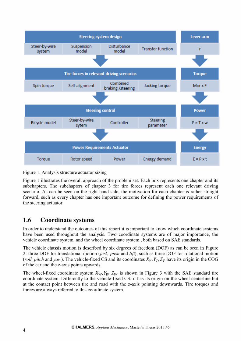
Figure 1. Analysis structure actuator sizing
Figure 1 illustrates the overall approach of the problem set. Each box represents one chapter and its
subchapters. The subchapters of chapter 3 for tire forces represent each one relevant driving
scenario. As can be seen on the right-hand side, the motivation for each chapter is rather straight
forward, such as every chapter has one important outcome for defining the power requirements of
the steering actuator.
1.6 Coordinate systems
In order to understand the outcomes of this report it is important to know which coordinate systems
have been used throughout the analysis. Two coordinate systems are of major importance, the
vehicle coordinate system and the wheel coordinate system , both based on SAE standards.
The vehicle chassis motion is described by six degrees of freedom (DOF) as can be seen in Figure
2: three DOF for translational motion (jerk, push and lift), such as three DOF for rotational motion
(roll, pitch and yaw). The vehicle-fixed CS and its coordinates have its origin in the COG
of the car and the z-axis points upwards.
The wheel-fixed coordinate system is shown in Figure 3 with the SAE standard tire
coordinate system. Differently to the vehicle-fixed CS, it has its origin on the wheel centerline but
at the contact point between tire and road with the z-axis pointing downwards. Tire torques and
forces are always referred to this coordinate system.
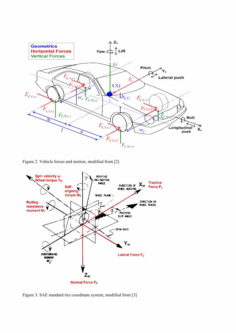
Figure 2. Vehicle forces and motion, modified from [2]
Figure 3. SAE standard tire coordinate system, modified from [3]

CHALMERS, Applied Mechanics, Master’s Thesis 2013:45 6
2 Steering system design
In this chapter the design of the overall steering system is presented. Covered is the whole system
from steering shaft, steering rack, rotational-linear transmissions etc. This covers mainly research
on existing systems and how they can be implemented/ adjusted to the EDV car.
Specific terms and abbreviations
handwheel angle [ ]
handwheel sensor/actuator angle [ ]
rotor angle/rate [ ]/[ ⁄ pinion angle/rate [ ]/[ ⁄
road wheel angle/rate [ ]/[ ⁄ steering rack displacement steering rack mass effective steering arm length steering ratio [-]
gear ratio [-]
torsion bar stiffness lumped inertia of rotor and coupling shaft about rotor shaft
[ ⁄ ]
lumped inertia of steering rack and wheels about steering axis
[ ⁄ ]
output rotor torque steering actuator (before gear transmission) [ lumped wheel torque about kingpin axis for both front wheels [ rotor damping ⁄
rack and tire damping about steering axis ⁄
2.1 Steer-by-wire setup
Figure 4. Steer-by-wire steering system design, modified from [4]
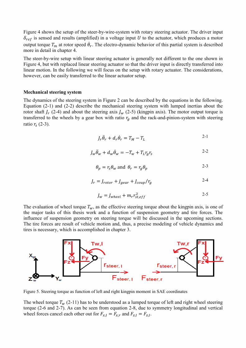
Figure 4 shows the setup of the steer-by-wire-system with rotary steering actuator. The driver input
is sensed and results (amplified) in a voltage input to the actuator, which produces a motor
output torque at rotor speed . The electro-dynamic behavior of this partial system is described
more in detail in chapter 4.
The steer-by-wire setup with linear steering actuator is generally not different to the one shown in
Figure 4, but with replaced linear steering actuator so that the driver input is directly transferred into
linear motion. In the following we will focus on the setup with rotary actuator. The considerations,
however, can be easily transferred to the linear actuator setup.
Mechanical steering system
The dynamics of the steering system in Figure 2 can be described by the equations in the following.
Equation (2-1) and (2-2) describe the mechanical steering system with lumped inertias about the
rotor shaft (2-4) and about the steering axis (2-5) (kingpin axis). The motor output torque is
transferred to the wheels by a gear box with ratio and the rack-and-pinion-system with steering
ratio (2-3).
2-1
2-2
and 2-3
⁄ 2-4
2-5
The evaluation of wheel torque , as the effective steering torque about the kingpin axis, is one of
the major tasks of this thesis work and a function of suspension geometry and tire forces. The
influence of suspension geometry on steering torque will be discussed in the upcoming sections.
The tire forces are result of vehicle motion and, thus, a precise modeling of vehicle dynamics and
tires is necessary, which is accomplished in chapter 3.
Figure 5. Steering torque as function of left and right kingpin moment in SAE coordinates
The wheel torque (2-11) has to be understood as a lumped torque of left and right wheel steering
torque (2-6 and 2-7). As can be seen from equation 2-8, due to symmetry longitudinal and vertical
wheel forces cancel each other out for and .

CHALMERS, Applied Mechanics, Master’s Thesis 2013:45 8
2-6
2-7
( ) ( ) ( ) 2-8
The wheels support each other, provided that there is a connecting steering rack between left and
right side. The wheel torque due to lateral forces, however, always add up. The relations stated
above are discussed more in detail throughout this work.
2.2 Suspension model
This chapter explains the general suspension geometry and how its parameter influence the wheel
torque . There are different suspension types, but they can all be described by same geometry
parameters. For the EDV the double-wish-bone suspension type has been chosen [5].
Abbreviations and specific terms
kingpin inclination
caster angle
effective kingpin angle
caster trail
pneumatic trail
caster offset on wheel center height
kingpin offset/ scrub radius
kingpin offset on wheel center height
camber angle
toe angle
wheel steer angle
Term Description
kingpin axis also referred to steering axis; this axis defines the wheel
turning center when changing the steering angle.
kingpin inclination inclination of steering axis in y-z-plane (see Figure 7)
caster angle steering axis inclination in x-z-plane (see Figure 6)
effective kingpin angle effective three-dimensional kingpin angle as sum of
inclination and caster angle √
caster trail the longitudinal distance between where the steering axis hits
the ground and the wheel center
pneumatic trail the longitudinal distance between wheel center and lateral
force acting point on tire contact patch plane
kingpin offset/ scrub radius the lateral distance between where the steering axis hits the
ground and the wheel center (negative if on outside of the
wheel)
camber angle inclination of wheels y-z-plane (see Figure 7)
toe angle tilt of wheels in x-y-plane (see Figure 6)
uprights uprights are the mounting parts, which connect wheels with
suspension parts and steering system. The brake system is also
mounted on the uprights.
wishbones Wishbones are part of the suspension system and connect
uprights with the vehicle chassis. They allow the wheels to
move in vertical direction during bumping and define the
degrees of freedom of the wheel.

Figure 6. Left: Determination of wheel angles, from [2], Right: Caster angle and
caster trail, from [6]
Figure 7. Left: Camber angle , from [6], Middle: Kingpin inclination, from [6], Right: Kingpin offset/ scrub
radius, from [6],
Suspension geometry model
The suspension geometry plays a major role in defining the forces on the steering rack. The relative
position of the kingpin axis to the wheel- as the rotating axis of the wheel with fixed relative
position to vehicle chassis - is described in this model. However, the assumption of a fixed relative
position of kingpin axis to vehicle chassis is not completely correct. Especially during vertical
wheel motion due to road bumps the relative position changes considerably. This fact is taken into
account by varying the geometrical parameters.
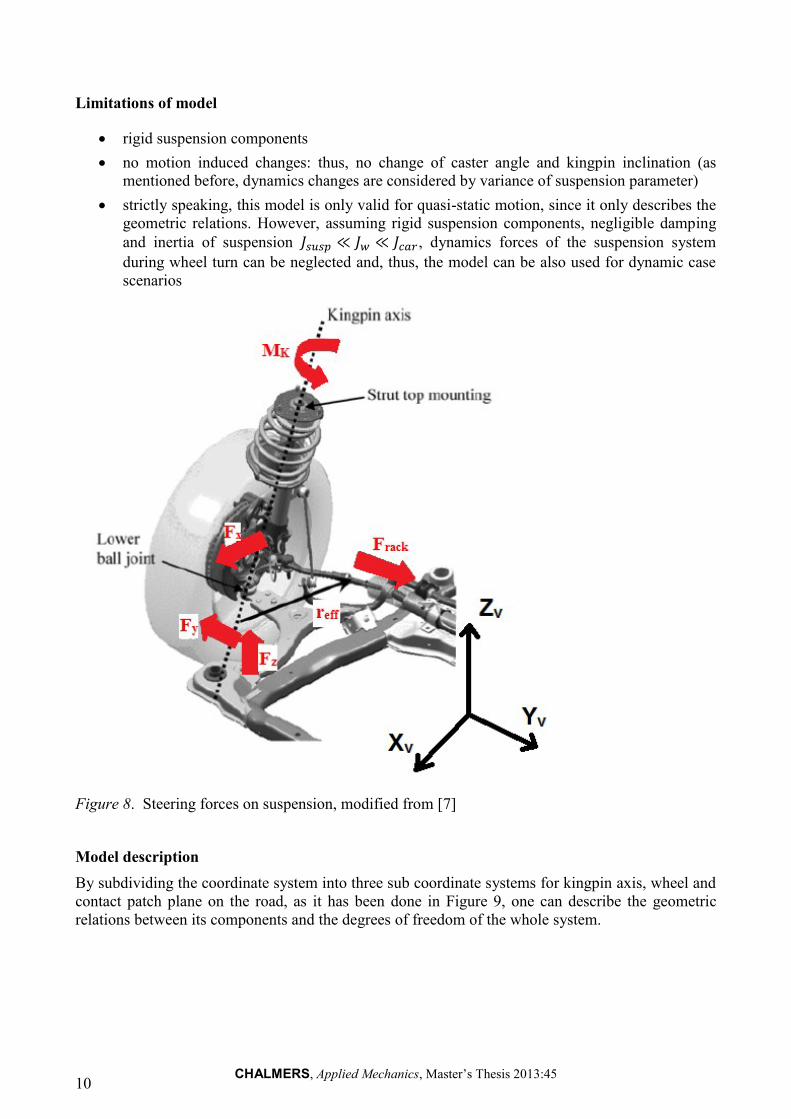
Forces in longitudinal, lateral and vertical direction produce a moment around the kingpin axis,
which results in the steering rack force (see Figure 8). Once, the forces acting on the wheel are
properly defined the steering rack force can be easily calculated. The model presented in the
following is based on the work of Cho [7].
CHALMERS, Applied Mechanics, Master’s Thesis 2013:45 10
Limitations of model
rigid suspension components
no motion induced changes: thus, no change of caster angle and kingpin inclination (as
mentioned before, dynamics changes are considered by variance of suspension parameter)
strictly speaking, this model is only valid for quasi-static motion, since it only describes the
geometric relations. However, assuming rigid suspension components, negligible damping
and inertia of suspension , dynamics forces of the suspension system
during wheel turn can be neglected and, thus, the model can be also used for dynamic case
scenarios
Figure 8. Steering forces on suspension, modified from [7]
Model description
By subdividing the coordinate system into three sub coordinate systems for kingpin axis, wheel and
contact patch plane on the road, as it has been done in Figure 9, one can describe the geometric
relations between its components and the degrees of freedom of the whole system.

Figure 9. , Suspension coordinate system, modified from [7]
Despite the three sub-coordinate-systems, displacement vectors , tire forces and kingpin vector
are in the vehicle coordinate system in equation 2-9 to 2-11. Since tire forces are
generally described in tire coordinates they have to be transferred in vehicle coordinates.
The longitudinal force can be sufficiently described by the force acting on the wheel center.
Differently to vertical and lateral force, does the wheel radius not affect the kingpin moment due to
longitudinal forces. For the side slip force and vertical force the force acting point at the tire-
with (
) 2-9
(
) 2-10
(
) 2-11

CHALMERS, Applied Mechanics, Master’s Thesis 2013:45 12
to-ground contact patch has to be considered. For each force acting point, the displacement vector (as can be seen in equation 2-9 to 2-11) is defined, from which the moment around the kingpin axis
is calculated.
Equation 2-12 shows the transformation between forces in the vehicle coordinate system
and wheel coordinate system using transformation matrix. The kingpin axis vector is
given in equation 2-13 for vehicle coordinates.
Using those relations, the kingpin moments due to longitudinal, lateral and vertical tire forces can
be simplified to 2-14, 2-15 and 2-18.
As can be seen from equation 2-14 to 2-16, does only the kingpin moment due to vertical
forces change with steering angle . This effect is known as car-lifting-effect. The lever arms of
lateral and longitudinal force are kept constant. One can see from equation 2-16, that the car-lifting-
effect only applies for and .
Influence of effective kingpin angle
The kingpin moment due to longitudinal, lateral and vertical tire forces is affected by caster angle
and kingpin inclination , expressed by the effective kingpin angle √ . The influence of
effective kingpin angle is described in equation 2-17 and 2-18.
2-17
2-18
Equation 2-17 and 2-18 show primarily the effects of effective kingpin inclination on torque
transmission between wheel torque and kingpin torque (steering torque). This means, the impact of
wheel forces and the steering effort to maintain force equilibrium on the wheels is reduced.
Simultaneously steering effort necessary to turn the wheels is increased. For a range of is this effect not much with steering effort change of roughly . However, we will see
in chapter 3, that the variation of caster and kingpin inclination also influences the forces and wheel
torque amplitude itself, which leads to considerable increment of steering effort.
Figure 10 below illustrates the geometric parameter of the kingpin axis. One should take in mind,
that the kingpin axis is a virtual axis, which is defined by the two mounting at the uprights and,
thus, scrub radius can be also negative, which can change sign of and .
(
)
(
)(
)
2-12
kingpin axis unit vector (
) 2-13
2-14
2-15
+ 2-16

Figure 10. Kingpin axis coordinates
2.3 Disturbance model
The disturbance model considers a change of lever arms due to the change of the force acting points
on the wheel. This can have crucial impact on the steering effort, since the suspension geometry is
generally designed for reducing the steering effort. This means, that the distance of kingpin axis to
force acting points is designed to be as small as possible for standard driving situations. As we will
see later in chapter 3 the change of force acting points on the wheel results also in considerable
change of tire forces and, hence the kingpin moment.
Figure 11 shows the change of force acting points on the tire due to disturbance for longitudinal,
lateral and vertical tire forces.

CHALMERS, Applied Mechanics, Master’s Thesis 2013:45 14
Figure 11. Left: Vertical and longitudinal shift of force acting point, Right: Lateral shift of force
acting point
Equation 2-19, 2-20 and 2-21 show that the decrease of contact patch area doesn’t increase steering
effort.
(
) 2-19
(
) 2-20
(
)
+
2-21
We can see again that the change of lever arm is independent of steering angle for and .
Despite the fact of the force shift (in the right-hand figure of Figure 11), one should also consider
the reduction of contact patch size during disturbance in Figure 12. The contact patch becomes
important when it comes to turning the wheel, as we will see in chapter 3. However, we can already
show at this point, that the reduction of contact patch area results also in a reduction of steering
torque, considering that tire forces stay the same due to unchanged wheel load (see equation 2-22 to
2-24).
Figure 12. Effects of lateral shift on static torque
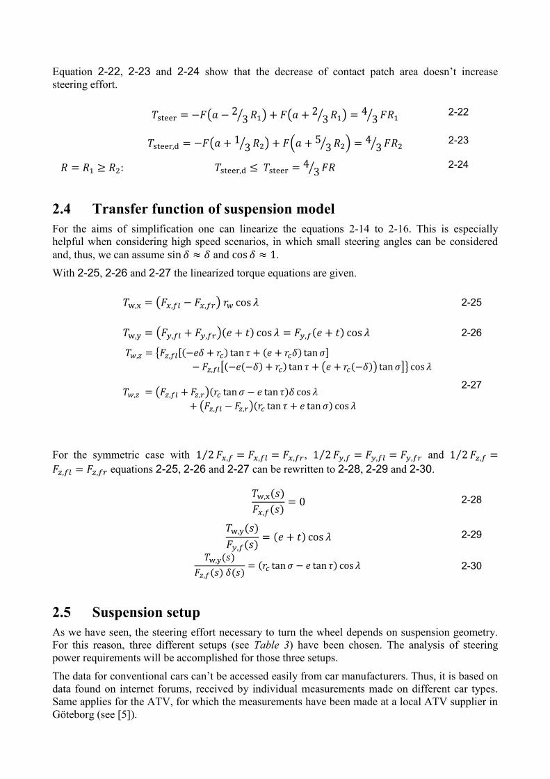
Equation 2-22, 2-23 and 2-24 show that the decrease of contact patch area doesn’t increase
steering effort.
( ⁄ ) (
⁄ ) ⁄ 2-22
( ⁄ ) (
⁄ ) ⁄ 2-23
⁄ 2-24
2.4 Transfer function of suspension model
For the aims of simplification one can linearize the equations 2-14 to 2-16. This is especially
helpful when considering high speed scenarios, in which small steering angles can be considered
and, thus, we can assume and .
With 2-25, 2-26 and 2-27 the linearized torque equations are given.
( ) 2-25
( ) 2-26
{
[ ( ) ]}
2-27
( )
( )
For the symmetric case with ⁄ , ⁄ and ⁄
equations 2-25, 2-26 and 2-27 can be rewritten to 2-28, 2-29 and 2-30.
2-28
2-29
2-30
2.5 Suspension setup
As we have seen, the steering effort necessary to turn the wheel depends on suspension geometry.
For this reason, three different setups (see Table 3) have been chosen. The analysis of steering
power requirements will be accomplished for those three setups.
The data for conventional cars can’t be accessed easily from car manufacturers. Thus, it is based on
data found on internet forums, received by individual measurements made on different car types.
Same applies for the ATV, for which the measurements have been made at a local ATV supplier in
Göteborg (see [5]).
CHALMERS, Applied Mechanics, Master’s Thesis 2013:45 16
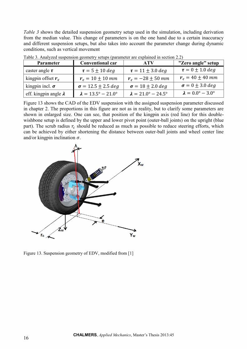
Table 3 shows the detailed suspension geometry setup used in the simulation, including derivation
from the median value. This change of parameters is on the one hand due to a certain inaccuracy
and different suspension setups, but also takes into account the parameter change during dynamic
conditions, such as vertical movement
Table 3. Analyzed suspension geometry setups (parameter are explained in section 2.2)
Parameter Conventional car ATV ”Zero angle” setup
caster angle
kingpin offset
kingpin incl.
eff. kingpin angle
Figure 13 shows the CAD of the EDV suspension with the assigned suspension parameter discussed
in chapter 2. The proportions in this figure are not as in reality, but to clarify some parameters are
shown in enlarged size. One can see, that position of the kingpin axis (red line) for this double-
wishbone setup is defined by the upper and lower pivot point (outer-ball joints) on the upright (blue
part). The scrub radius should be reduced as much as possible to reduce steering efforts, which
can be achieved by either shortening the distance between outer-ball joints and wheel center line
and/or kingpin inclination .
Figure 13. Suspension geometry of EDV, modified from [1]
3 Tire forces
This chapter provides the analysis of tire forces in relevant driving situations. Better speaking, the
following chapter considers various load case scenarios for which maximum power requirements on
steering actuator are expected. This is accomplished by analyzing the tire forces in specific driving
scenarios. Hence, the following subchapters can be each seen as a separate driving scenario.
3.1 Driving scenarios
Relevant for defining critical driving scenarios is understanding of the relation between steering
torque on right and left steered wheel. Generally speaking for longitudinal and vertical wheel
forces, the steering effort is proportional to the difference between resulting kingpin moments on
left and right wheel. The kingpin moments due to lateral forces, however, add up due to the same
acting direction of lateral forces during cornering.
Thus, driving situations have to be identified, in which forces on right and left wheel counter-act or
the great difference between left and right wheel kingpin moment occur.
1. Spin torque in parking conditions: Steering effort to turn the wheels in stand-still conditions is
increased due to the relaxation length of the tire and, thus, maximum steering torque to spin the
wheels, occurs at . This effect is further explained in the upcoming section and the
evaluation of maximum static torque is shown in section 3.3.
2. Lateral tire forces in high-speed cornering: As has been described before, lateral tire forces
differ from the impact of longitudinal and vertical tire forces, since their kingpin moments
generally add up due to the same acting direction of . increases with increased lateral
acceleration and, thus, with increased cornering speed. The kingpin moment due to
lateral forces is often referred to the term self-alignment-torque, since it results in the wheels
keeping straight-line direction. However, it will be shown in chapter 3.4, that there is a peak
value before reaches its maximum due to a reduction of pneumatic trail.
The influence of caster trail on kingpin moment has been discussed in chapter 2 already in
terms of suspension geometry. In relation to self-alignment torque it is worth it looking into it
again, since the presence of constant caster trail leads to a considerable change of the alignment
torque characteristic. The standard model shows that alignment torque becomes zero when the
tires are saturated. The saturated tire still produces lateral tire forces, though, which is why with
caster trail still a high alignment torque is present at high slip angles.
3. Combined steering and braking: Combined steering and braking is a common driving
scenario, especially in emergency braking. Kingpin moment and occur at the same
instant of time, which increases the overall steering torque. Nevertheless, in this scenario the tire
saturation has major impact, since sum of longitudinal and lateral tire forces is restricted by the
physical limits of the tire.
4. Dynamic wheel load on bumpy roads: During driving on bumpy road considerably high
vertical wheel loads occur. Those forces are strongly influenced by the vehicle parameters, such
as suspension stiffness and damping, tire properties, sprung- to unsprung-mass ratio, etc. For
defining the forces a detailed analysis of vertical dynamics is necessary, which can be found in
APPENDIX A. The influence of different suspension geometry setups can be found in chapter
3.7
CHALMERS, Applied Mechanics, Master’s Thesis 2013:45 18
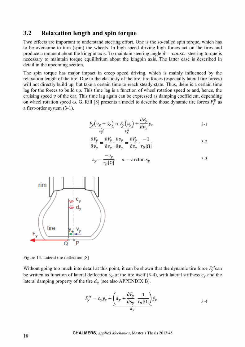
3.2 Relaxation length and spin torque
Two effects are important to understand steering effort. One is the so-called spin torque, which has
to be overcome to turn (spin) the wheels. In high speed driving high forces act on the tires and
produce a moment about the kingpin axis. To maintain steering angle steering torque is
necessary to maintain torque equilibrium about the kingpin axis. The latter case is described in
detail in the upcoming section.
The spin torque has major impact in creep speed driving, which is mainly influenced by the
relaxation length of the tire. Due to the elasticity of the tire, tire forces (especially lateral tire forces)
will not directly build up, but take a certain time to reach steady-state. Thus, there is a certain time
lag for the forces to build up. This time lag is a function of wheel rotation speed and, hence, the
cruising speed of the car. This time lag again can be expressed as damping coefficient, depending
on wheel rotation speed . G. Rill [8] presents a model to describe those dynamic tire forces as
a first-order system (3-1).
Figure 14. Lateral tire deflection [8]
Without going too much into detail at this point, it can be shown that the dynamic tire force can
be written as function of lateral deflection of the tire itself (3-4), with lateral stiffness and the
lateral damping property of the tire (see also APPENDIX B).
( )⏟
( )⏟
3-1
| | 3-2
| | 3-3
(
| |)
⏟
3-4

We can see, that the new damping coefficient is now also a function of cornering stiffness
and wheel rotation speed and will decrease with increasing velocity. Equation 3-5describes the
force equilibrium in point Q in Figure 14.
From there, the kingpin torque due to lateral force can be calculated. Basically, this explains
why spin torque decreases with increased velocity and why wheel turn in parking situation requires
the most steering effort.
To explain this effect, it was necessary to approach the problem form wheel dynamics perspective
with the lateral deflection of the tire. In the following sections dynamic tire forces are described in
terms of tire slip and the forces between tire and ground. The relation between both is given by
equilibrium in point Q in. From now on the tire itself will be assumed to be stiff and tire deflection
will be considered by cornering stiffness and damping .
3.3 Spin torque in static conditions
R.Sc. Sharp and R. Granger [9] developed an empirical formula for static torque prediction around
the kingpin axis in stand-still situations. It is based on a model in physical macro-scale and
integrates friction forces over a circular contact patch.
Specific terms Description
tire friction the effect of tire slip forces in longitudinal and lateral direction due to
shear stress as a result of deformation of tire and profile elements
tire stiction the effect of sudden reduction of friction forces due to tire saturation
Limitations of model
The model restricted by the following assumptions and limitations:
Perfectly circular contact patch
Pressure is equally distributed over contact patch (correction factor in equation 3-9)
Torque center coincides with contact patch center
No stiction effects considered (friction based on experimentally obtained coefficient)
Zero caster angle and zero kingpin inclination: lever arms stay constant during wheel turn
Model
The model of R.Sc. Sharp and R. Granger [9] considers a circular contact patch, as can be seen in
Figure 15.
Figure 15. Static torque due to friction forces in circular contact patch plane
3-5

CHALMERS, Applied Mechanics, Master’s Thesis 2013:45 20
The model evaluates the static torque by analyzing the tire-to-ground friction over the whole contact
patch. In equation 3-6 the tire friction forces are summed up over the contact patch. The parameters
are given in Table 4.
∫ ∫
∫
3-6
3-7
Table 4. Static tire model parameters
Term Description
contact patch radius
friction force of infinite contact patch element
static wheel load
internal tire pressure
effective tire-to-ground pressure empirical correction factor
(R. Granger suggest ;depends on tire type)
The friction force and its resulting static torque of each infinite small
element of the contact patch plane is integrated about the whole contact surface in
Equation 3-6. By equation 3-7 the contact patch center radius can be eliminated, which leads to
expression 3-8. Equation 3-8 is independent of the size of the contact patch, since it is assumed that
the pressure is evenly distributed on the patch.
√
3-8
√
3-9
Equation 3-9 contains an empirical correction factor since for low tire pressures, the tire-to-
ground contact pressure will be greater at the edges of the contact area and lesser in the middle. The
converse will be true for high inflation pressures.
The given formula is a function of the three parameters tire inflation pressure, wheel load and tire-
to-road friction. The authors could experimentally show that it builds up the reality in good
approximation for normal stand-still conditions and that the static torque is independent of the scrub
radius. This is due to the compensation of the lever arm increment with the ability of the wheel to
roll with increased lever arm , which has been shown in [9]. This is only valid for the non-locked
wheel case, as described in the following.
Figure 16. Change of static torque lever arm due to caster trail and scrub radius
Equation 3-8 considers only zero caster trail. To show the effect of spin center offset equation 3-8
has to be slightly modified. If we consider both, caster trail and scrub radius , it can be seen in
Figure 16, that the effective lever arm changes from (3-10) to (3-11).
⏟
⏟
3-10
( )
[ (
)] 3-11
The static spin torque equation can then be rewritten to 3-12:
∫ ∫
√ (
) 3-12
Hence, static spin torque changes by the factor (equation 3-13), with and .
√
√ (
)
√
3-13
For free rolling wheels factor reduces to √ , so that spin torque is independent
of scrub radius . However, if we consider locked wheels, the change of scrub radius has impact on
static spin torque and we have to use √ (
).
If we consider further the locked wheel case or driving up a curb, one could consider longitudinal
tire force as a function of motor torque. However, if we consider that motor torque is , we can show that ⁄ . In section 3.6 the case of
tire force will be considered, so that no additional considerations are necessary at this
point.
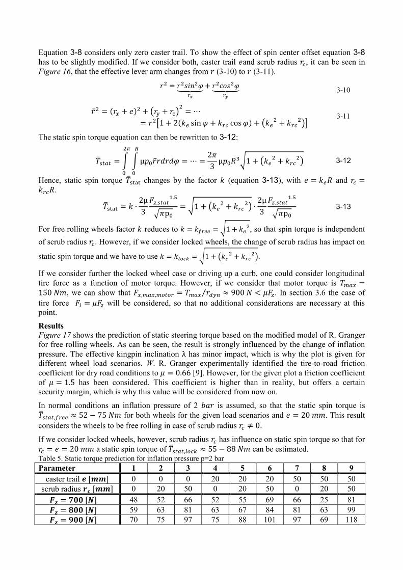
Results
Figure 17 shows the prediction of static steering torque based on the modified model of R. Granger
for free rolling wheels. As can be seen, the result is strongly influenced by the change of inflation
pressure. The effective kingpin inclination has minor impact, which is why the plot is given for
different wheel load scenarios. W. R. Granger experimentally identified the tire-to-road friction
coefficient for dry road conditions to [9]. However, for the given plot a friction coefficient
of has been considered. This coefficient is higher than in reality, but offers a certain
security margin, which is why this value will be considered from now on.
In normal conditions an inflation pressure of 2 is assumed, so that the static spin torque is
for both wheels for the given load scenarios and . This result
considers the wheels to be free rolling in case of scrub radius .
If we consider locked wheels, however, scrub radius has influence on static spin torque so that for
a static spin torque of can be estimated. Table 5. Static torque prediction for inflation pressure p=2 bar
Parameter 1 2 3 4 5 6 7 8 9
caster trail 0 0 0 20 20 20 50 50 50
scrub radius 0 20 50 0 20 50 0 20 50
48 52 66 52 55 69 66 25 81
59 63 81 63 67 84 81 63 99
70 75 97 75 88 101 97 69 118

CHALMERS, Applied Mechanics, Master’s Thesis 2013:45 22
Figure 17. Results of static torque prediction for both free rolling wheels with
Figure 18. Results of static torque prediction for both locked wheels with

3.4 Lateral tire forces at high speed
The biggest difference between high speed and low speed scenarios is the influence of lateral
acceleration on tire forces. In high speed driving the force necessary to maintain equilibrium
state of the wheel to (stationary conditions with constant wheel angle ) is the greatest.
The spin torque decreases with increased speed due to increase of relaxation length. Of course,
dynamic (non-stationary) conditions play a major role for defining the dynamic steering actuator
forces necessary for a certain reaction time. However, for describing just the tire forces in high
speed driving the stationary case is sufficient.
Longitudinal and lateral tire forces are mostly described by friction coefficient , which is a
function of tire slip and is defined as tire force over normal load , which is shown in (3-14).
The tire slip is defined as tire slip velocity over tire peripheral speed | | (3-15).
( )
3-14
| |
| | 3-15
Lateral slip is usually expressed with slip angle . Figure 19 shows a typical -slip-curve for
longitudinal tire force.
Figure 19. -slip-curve, modified from [2]
The curve shape for lateral tire force is slightly different, but the characteristic is the same. The tire
force reaches its maximum at comparably low slip and then decreases with further slip increase.
The zone after maximum tire friction is referred to as tire saturation zone, since the tire saturates
and is not able to build up greater tire force.
For the purpose of simplification the -slip-curve for lateral tire force is often linearized in the zone
below peak friction. This is by introducing cornering stiffness so that lateral tire force can
be expressed as function slip angle (3-16). The cornering stiffness is only valid for small slip
angles (3-17).
3-16
|
3-17

CHALMERS, Applied Mechanics, Master’s Thesis 2013:45 24
For high speed driving it is often only of interest to analyze vehicle behavior at small slip angles
only until maximum tire force and, hence, the -slip-curve is linearized in that region. The
cornering stiffness is defined as the gradient of the -slip-curve at zero. In the upcoming
sections we will use the cornering stiffness to describe lateral tire force.
Brush tire model
For the estimation of performance requirements of the steering actuators for the EDV we are
interested in a simple tire model, which allows us to estimate peak forces and velocities. For this
purpose, no complex thermo-mechanical or FEM tire model is necessary. Besides that, it is
extremely difficult and expensive to acquire precise tire data from the manufacturers. Thus, the
decision was taken to use the so-called brush tire model based on physical macro-scale, which
requires longitudinal and lateral stiffness only and some assumption on geometric dimensions of the
contact patch, as has been done already in the creep-speed evaluation. Formulas and picture of the
standard tire brush model in the following are taken from Paceijka [10].
Figure 20. Brush model principle (pure side slip), from [10]
The brush tire model describes the tire as a circular row of elastic bristles, which when touching the
road plane, deflect in a direction parallel to the road surface (see left-hand side Figure 20). The
basic principle is that it differentiates between an adhesion region and a sliding region of the contact
patch. In the adhesion region maximum deflection is not reached yet and friction force still
increases linearly with increased deflection. In the sliding region maximum deflection is already
reached and a further increase of tire force is not possible due to physical capacity of the tire. The
brush model assumes the pressure distribution over the contact patch and, thus, the maximum
deflection to vary according to a parabola. Starting with the rear part of the contact patch to
slide (case A right-hand side of Figure 20), the sliding region will increase with increasing
longitudinal slip or side slip until the tire is finally saturated and the total contact patch slides
(case D right-hand side of Figure 20).

Brush model for pure lateral slip
Since we’re mainly interested in lateral tire force due to mayor impact on kingpin moment in
high-speed, we will focus first on the pure side slip case. In Figure 21 the maximum possible lateral
deformation ⁄ is indicated, with lateral force distribution and lateral stiffness
.
Figure 21. Brush model moving at pure side slip, from [10]
With the lateral stiffness of the tread elements per unit length and lateral deformation for
vanishing sliding and (3-18), one can define cornering force (3-19) and self-
aligning torque (3-20) and consequently cornering stiffness (3-21) and aligning stiffness
(3-22).
3-18
∫
3-19
∫
3-20
(
)
3-21
(
)
3-22
For the case of finite and greater slip angle , the sliding region will appear and the largest
possible side force is limited. As mentioned before, the brush model assumes a parabolic
distribution of the vertical force per unit length (3-23) and, hence, the largest possible side force
distribution (3-24).

CHALMERS, Applied Mechanics, Master’s Thesis 2013:45 26
{ (
)
} 3-23
| |
3-24
The brush model now differentiates between the adhesion and sliding region by defining the point
at which the deflection of the adhesion region becomes equal to that of the sliding region. The
equation are normalized by introducing the composite tire model parameter . By introducing the
variable , by using equation equilibrium at (3-18, 3-23, 3-25) the slip angle at which
total sliding starts ( ) can be defined (3-27).
3-25
| | 3-26
3-27
From there, using for the side slip, cornering force (3-28), aligning torque (3-29)
and pneumatic trail (3-30) can be defined. The pneumatic trail for vanishing slip (3-19, 3-20) is
given by ( ⁄ )
⁄ . Pacejka [10] adds, that the introduction of an elastic
carcass will more likely improve this value to .
{ { | |
( )
}
| |
| | ⁄ 3-28
{
{ | | ( ) | |
}
| |
| | ⁄
3-29
{
| | ( ) | |
| | ( )
| |
| | ⁄
3-30
From equation 3-29 the peak value (3-31) can be found.
(
) (at
) 3-31
This value is of interest for the sizing of steering actuators for the EDV. Due to normalizing, those
results can be generalized and applied to the EDV tires by defining wheel load , contact patch
length composite tire model parameter and friction coefficient . The lateral stiffness can
be defined by a given cornering stiffness using equation 3-21. Pacejka [10] uses the correlation 3-32
between contact patch and vertical load, based on the assumption that 2a changes by the power of
two with radial tire deflection and the linear dependency to wheel load . Then the peak
value can be written as (3-33).
3-32
(
√
)
⁄ 3-33
Comparing the maximum alignment torque with the static torque for 2 bar
inflation pressure from equation 3-8, we can see that the estimated magnitude of alignment torque is
about one third of the static torque magnitude (3-34).
3-34
Pacejka itself states and shows experimentally, that the magnitude of the tire brush model is at
about four fifth of the actual self-alignment torque | |
| | [10]. Comparing with
real tire measurements available from the website of Avonracing (compare [11] and APPENDIX
D), which have been accomplished for formula student racing tires with wheel load
, we can see that the calculated relative magnitude | | in is of magnitude of
those measurements.
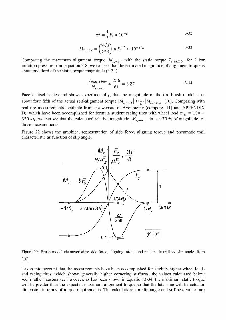
Figure 22 shows the graphical representation of side force, aligning torque and pneumatic trail
characteristic as function of slip angle.
Figure 22: Brush model characteristics: side force, aligning torque and pneumatic trail vs. slip angle, from
[10]
Taken into account that the measurements have been accomplished for slightly higher wheel loads
and racing tires, which shown generally higher cornering stiffness, the values calculated below
seem rather reasonable. However, as has been shown in equation 3-34, the maximum static torque
will be greater than the expected maximum alignment torque so that the later one will be actuator
dimension in terms of torque requirements. The calculations for slip angle and stiffness values are
CHALMERS, Applied Mechanics, Master’s Thesis 2013:45 28
based on tire brush model formulas and the cornering stiffness value for low wheel load tire from
Nicholas D. Smith [3], which evaluated the used reference tire data from [11].
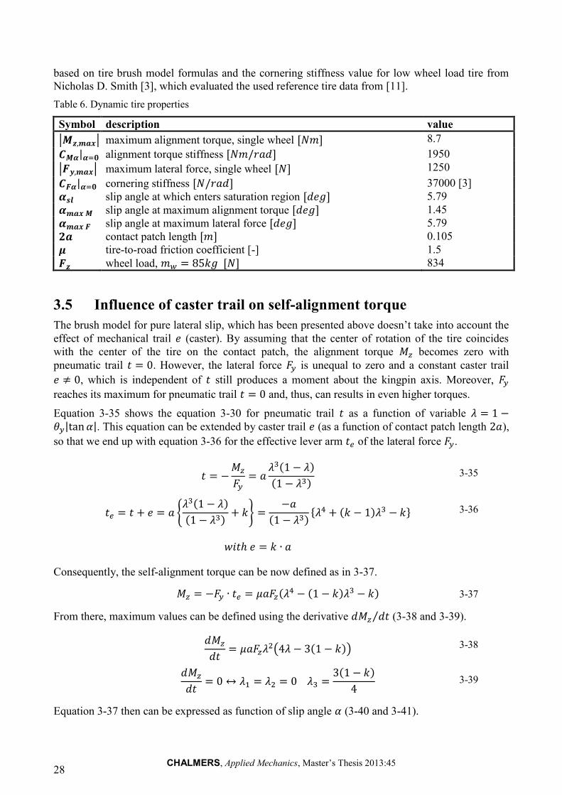
Table 6. Dynamic tire properties
Symbol description value
| | maximum alignment torque, single wheel 8.7
| alignment torque stiffness 1950
| | maximum lateral force, single wheel 1250
| cornering stiffness 37000 [3]
slip angle at which enters saturation region 5.79
slip angle at maximum alignment torque 1.45
slip angle at maximum lateral force 5.79
contact patch length 0.105
tire-to-road friction coefficient [-] 1.5
wheel load, 834
3.5 Influence of caster trail on self-alignment torque
The brush model for pure lateral slip, which has been presented above doesn’t take into account the
effect of mechanical trail (caster). By assuming that the center of rotation of the tire coincides
with the center of the tire on the contact patch, the alignment torque becomes zero with
pneumatic trail . However, the lateral force is unequal to zero and a constant caster trail
, which is independent of still produces a moment about the kingpin axis. Moreover,
reaches its maximum for pneumatic trail and, thus, can results in even higher torques.
Equation 3-35 shows the equation 3-30 for pneumatic trail as a function of variable | |. This equation can be extended by caster trail (as a function of contact patch length ),
so that we end up with equation 3-36 for the effective lever arm of the lateral force .
3-35
{
}
{ } 3-36
Consequently, the self-alignment torque can be now defined as in 3-37.
3-37
From there, maximum values can be defined using the derivative ⁄ (3-38 and 3-39).
( ) 3-38
3-39
Equation 3-37 then can be expressed as function of slip angle (3-40 and 3-41).

| |
3-40
| | (
)
3-41
One can see, that for zero caster trail we end up with the original expressions | | and (compare 3-31).
The plot in Figure 23 shows the effects of increasing caster trail , which results in both, an
increasing alignment torque and the increment of , at which maximum occurs.
Figure 23. Normalized curves of self-alignment torque and effective lever arm for increasing caster
trail
Blue shows the normalized lever arm ⁄ and green the normalized alignment torque ⁄ . As reference, blue and green dashed lines show the curves of Figure 22 for zero
caster trail.
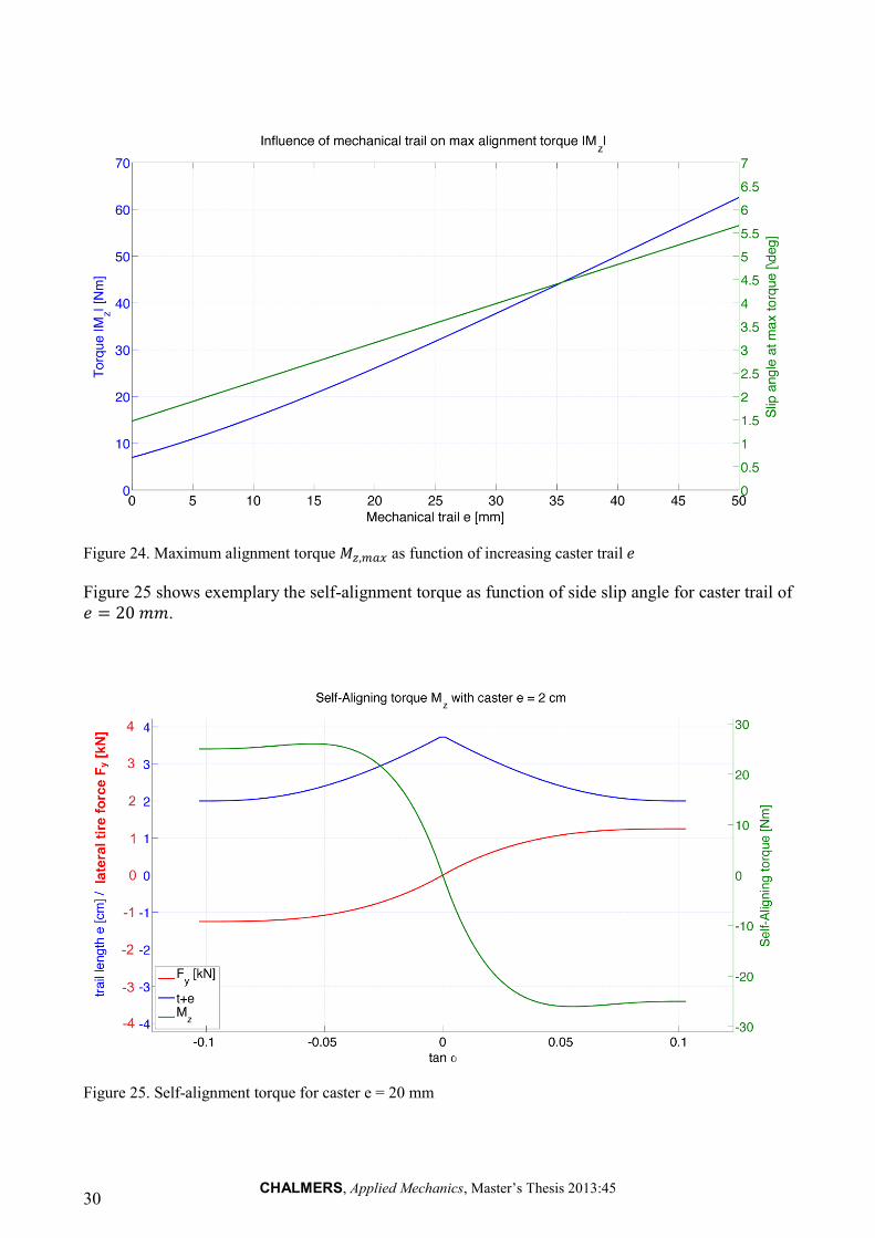
Figure 24 on the next page shows the effect of increasing caster trail on the peak
torque | | and the shift of to higher slip angles in effective numbers. While peak torque
changes nonlinear for small caster trail, changes almost linear over the whole range. It can be
seen that the impact of the consideration of caster trail is tremendous, which becomes obvious when
we consider that pneumatic trail at is only ⁄ .
The maximum value for the caster trail is not randomly chosen. What we can see is, that for
the angle, at which the peak torque occurs, is , which equals the tire
saturation slip angle . This means, for higher values of caster, the alignment torque will
still increase due to lever arm increment, but the tire force can’t increase anymore so that the torque
can’t increase so much anymore. However, greater caster trail is strongly not recommended. For 13
inch tires 50 mm caster trail equals caster angle .
CHALMERS, Applied Mechanics, Master’s Thesis 2013:45 30
Figure 24. Maximum alignment torque as function of increasing caster trail
Figure 25 shows exemplary the self-alignment torque as function of side slip angle for caster trail of
.
Figure 25. Self-alignment torque for caster e = 20 mm

3.6 Combined steering and braking
During combined steering and braking concurrently lateral forces and longitudinal braking force
produce a moment about the kingpin axis. This can result in a reduction of the overall kingpin
moment, but also result in the sum of both moments. This depends on the wheel side of the car and
the steering direction, but also on the position of the kingpin axis, which defines whether a braking
force produces a negative or positive kingpin moment. We will consider the “worst case” scenario
at which both moments will sum up. For more information on this steering case, see also [2] and
[12].
Equation 3-42 gives the summation of kingpin moment for one single wheel.
3-42
The kingpin moments will add up, the forces have different sign due to convention. In the combined
steering and braking scenario are longitudinal force and lateral force dependent on each other.
The combined resulting tire can’t be greater than the physical limitations of the tire (3-43).
√
3-43
This effect is typically described by the Kamm friction circle in Figure 26.
Figure 26. Kamm friction circle for EDV car and tire
The radius of the friction circle in Figure 26 can be shown normalized as one or can show the actual
physical limitation of the tire (for values of Table 6 on page 28). Both,
slip vector and resulting force vector can plotted as function of slip angle (3-44 to 3-46).
√
3-44

CHALMERS, Applied Mechanics, Master’s Thesis 2013:45 32
3-45
3-46
Measurements show that the relation between and is better described by a friction ellipse, but
for the purpose of maximum steering forces the friction circle is sufficient since it just slightly
overestimates the forces.
Using the friction circle one can also express the kingpin moment as function of (3-47).
To achieve this one must also express lateral force lever arm as function of , which
changes due to the change of pneumatic trail with slip angle . For this purpose, equation 3-36 for
is linearized to change linear with and then for small angles expressed as
function of slip angle (3-48).
Using relation 3-49 between and , the lever arm can then be expressed as function of
(3-50).
Simulation shows a very close correlation function 3-50 with the function 3-36 for of the brush
model becomes slightly overestimated, but since can be comparibly small to this doesn’t take
too much into account.
Figure 27. Linearization of lever arm
Figure 28 shows the results of the analysis of kingpin moment for combined steering and
braking, which has been done for different caster and kingpin angle setups.
The left-hand plot of Figure 28 shows plotted versus , which makes it easy to evaluate
kingpin moments on each wheel for different driving cases, such as right turn, left turn, traction,
braking and their combinations. The right-hand plot shows the summation of both as function of .
3-47
[
]
[
] 3-48
3-49
[
| |] 3-50

Figure 28. Results of steering torque effort in combined steering and braking for steered left wheel in ISO wheel coordinate system
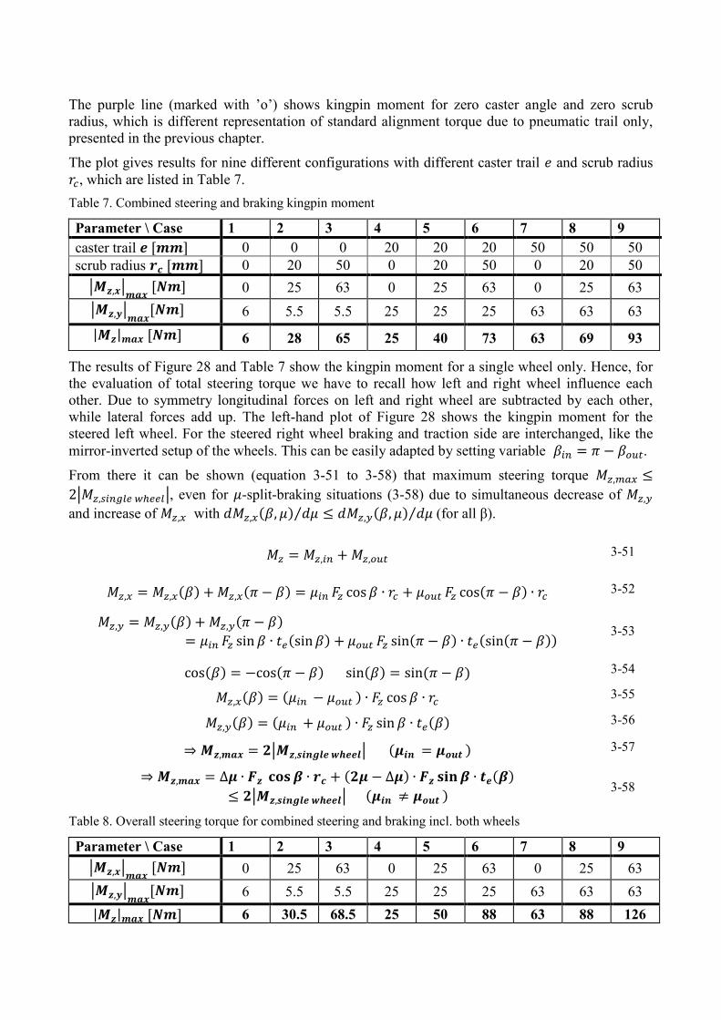
The purple line (marked with ’o’) shows kingpin moment for zero caster angle and zero scrub
radius, which is different representation of standard alignment torque due to pneumatic trail only,
presented in the previous chapter.
The plot gives results for nine different configurations with different caster trail and scrub radius
, which are listed in Table 7.
Table 7. Combined steering and braking kingpin moment
The results of Figure 28 and Table 7 show the kingpin moment for a single wheel only. Hence, for
the evaluation of total steering torque we have to recall how left and right wheel influence each
other. Due to symmetry longitudinal forces on left and right wheel are subtracted by each other,
while lateral forces add up. The left-hand plot of Figure 28 shows the kingpin moment for the
steered left wheel. For the steered right wheel braking and traction side are interchanged, like the
mirror-inverted setup of the wheels. This can be easily adapted by setting variable .
From there it can be shown (equation 3-51 to 3-58) that maximum steering torque
| |, even for -split-braking situations (3-58) due to simultaneous decrease of
and increase of with ⁄ ⁄ (for all β).
Table 8. Overall steering torque for combined steering and braking incl. both wheels
Parameter \ Case 1 2 3 4 5 6 7 8 9
caster trail 0 0 0 20 20 20 50 50 50
scrub radius 0 20 50 0 20 50 0 20 50
| | 0 25 63 0 25 63 0 25 63
| | 6 5.5 5.5 25 25 25 63 63 63
| | 6 28 65 25 40 73 63 69 93
3-51
3-52
3-53
3-54
3-55
3-56
| | 3-57
| | 3-58
Parameter \ Case 1 2 3 4 5 6 7 8 9
| | 0 25 63 0 25 63 0 25 63
| | 6 5.5 5.5 25 25 25 63 63 63
| | 6 30.5 68.5 25 50 88 63 88 126

3.7 Vertical wheel load and jacking torque
The vertical wheel load has to effects on the steering effort. On the one side it defines the
longitudinal and lateral tire forces and on the other side produces it a kingpin moment . The
equation for kingpin moment has been already developed in chapter 2 (equation 2-27) and
depends in comparison to the moment of longitudinal and lateral forces also on steering angle
(3-59).
For symmetric load ( ) and driving ( ) case kingpin moment will be zero
(3-60).
The same applies for zero caster trail and zero scrub radius (3-61). Hence, the static load case can
be neglected.
The greatest wheel load occurs for dynamic conditions anyways. Defining those dynamic wheel
forces is rather difficult, since it depends a lot on the suspension setup and the wheel weight. At this
stage of the project the decision for components has not been finalized yet, which makes even more
difficult. Also the considered driving scenario is important.
Generally, high vertical wheel loads occur during driving on bumpy roads. Peak forces occur when
the car gets excited in its natural frequency, which leads to resonance and high acceleration and
wheel load. Thus, hitting a single bump is a dimensioning driving scenario due to the wide
frequency spectrum of the impulse like input. Estimating maximum vertical forces is described
more in detail in APPENDIX A, in which the vertical dynamics analysis is performed. Vertical
forces on the wheel can be considerably greater than those in longitudinal and lateral direction. The
analysis showed that vertical forces up to can be reached, which is in the same
range as values stated in literature. A common thumb-rule is [1].
For high speed driving equation 3-59 can be simplified by setting steering angle , so that we
get equation 3-62.
For maximum torque a single-sided bump occurrence is considered with and
. Again, the same nine different configurations as in the previous section are considered.
In case of it is worth considering a negative scrub radius setup, since this can reduce the torque
amplitude a lot. Hence, one should notice that in this case it’s is not recommended to have zero-
trail-setup. Figure 29 shows graphically those results for the nine different suspension
configurations.
( )
( ) 3-59
( ) 3-60
3-61
( ) 3-62

CHALMERS, Applied Mechanics, Master’s Thesis 2013:45 36
Figure 29. Kingpin moment due to vertical wheel forces
We can see that negative scrub radius has considerable effect on the amplitude. Thus, a negative
scrub radius is highly recommended. The numerical results are shown in Table 9.
Table 9. Overall steering torque for vertical force impact
Parameter 1 2 3 4 5 6 7 8 9
caster trail 0 0 0 20 20 20 50 50 50
scrub radius 0 20 50 0 20 50 0 20 50
| | 0 35 88 17 53 106 44 79 132
scrub radius 0 -20 -50 0 -20 -50 0 -20 -50
| | 0 35 88 17 18 71 44 8 44
3.8 Effects of vertical load transfer during cornering
Due to roll in high speed cornering vertical wheel load increases on outer wheels in same amount as
it decreases on inner wheels, which leads at the same time to increase of tire force on outer wheel
and decrease on inner wheel.
One can show, that this effect in terms of lateral tire forces doesn’t increase steering effort, since
cornering stiffness is linear proportional (for small ) to wheel load change. Thus, steering effort
stays constant due to increase on outer wheel and decrease on the inside wheel. At higher wheel
loads the relation between cornering stiffness and wheel load is nonlinear and, hence, steering effort
even decreases (compare plots in APPENDIX C).
As has been shown before, steering effort due to longitudinal tire forces only occurs for different
tire forces on left and right steered wheel. Thus, steering effort will increase with vertical load shift.
However, one can show that this effect has less impact than the cases considered in the previous
sections.

Same can be shown for vertical wheel impact. Since one-sided road disturbance with dynamic
wheel load ( has been considered already, the impact of vertical load shift can
be considered less.
3.9 Conclusions
The results of this analysis showed that the effect of suspension geometry has major impact on
kingpin torque due to lateral, longitudinal and vertical tire forces. Static torque due to high spin
torque requires generally greatest steering effort. However, due to combination of steering toque in
high speed those forces can add up to even higher effort. Jacking torque can be quite high due to
great vertical forces, but its amplitude can be reduced through negative scrub radius. Thus, this
setup is strongly recommended.
For the modeling of steering control alignment torque can be modeled with different cornering
stiffness
and alignment torque stiffness
for the evaluated suspension setups
(refer to last rows of Table 10). In that case, the wheel torque changes linearly with increased slip
angle. For spinning and jacking torque there is no slightly increase of kingpin moment, so that they
can be modeled as steering step response.
CHALMERS, Applied Mechanics, Master’s Thesis 2013:45 38
4 Steering control
This chapter shows the design of the steering control system and which parameters that influence its
performance.
4.1 General control design
In order to evaluate the power requirements of the steering actuator a steering control loop is
necessary. Aim of the steering control is to make sure that time lag and amplitude difference in
wheel angle is small. Hence, the wheel angle should follow the driver’s steer intention,
described with as close as possible.
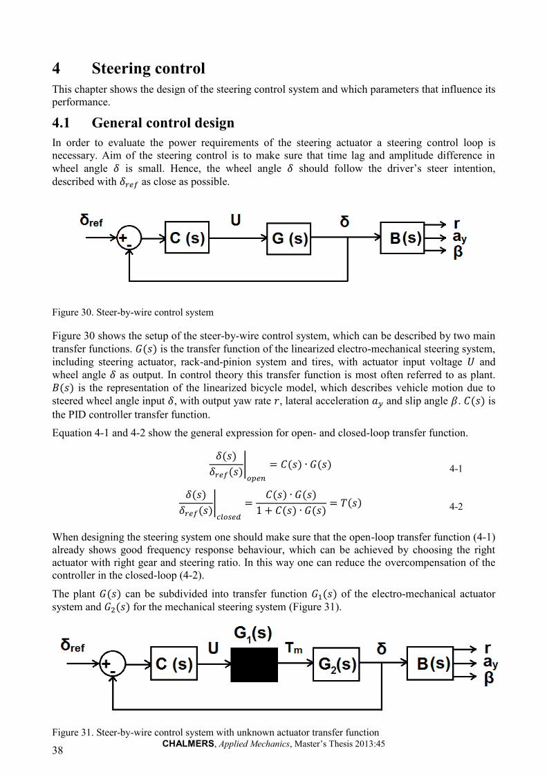
Figure 30. Steer-by-wire control system
Figure 30 shows the setup of the steer-by-wire control system, which can be described by two main
transfer functions. is the transfer function of the linearized electro-mechanical steering system,
including steering actuator, rack-and-pinion system and tires, with actuator input voltage and
wheel angle as output. In control theory this transfer function is most often referred to as plant.
is the representation of the linearized bicycle model, which describes vehicle motion due to
steered wheel angle input , with output yaw rate , lateral acceleration and slip angle . is
the PID controller transfer function.
Equation 4-1 and 4-2 show the general expression for open- and closed-loop transfer function.
When designing the steering system one should make sure that the open-loop transfer function (4-1)
already shows good frequency response behaviour, which can be achieved by choosing the right
actuator with right gear and steering ratio. In this way one can reduce the overcompensation of the
controller in the closed-loop (4-2).
The plant can be subdivided into transfer function of the electro-mechanical actuator
system and for the mechanical steering system (Figure 31).
Figure 31. Steer-by-wire control system with unknown actuator transfer function
|
4-1
|
4-2
This separation is especially helpful since most manufactures present information about their
actuators as black-box with the relation between input voltage and output torque . However, in
the following sections the transfer function of the whole steering system will be developed to
explain the influence of its parameters.
Obviously there is interaction between steering motion and vehicle motion . For
simplicity this interaction will be modeled in the following as inertia , damping and stiffness
of steering angle . With that simplification those subsystems can be handled more or less
independent from each other. Using those parameters allows us to describe steering forces in
driving scenarios, for which the bicycle model is not valid anymore.
4.2 Bicycle model transfer function
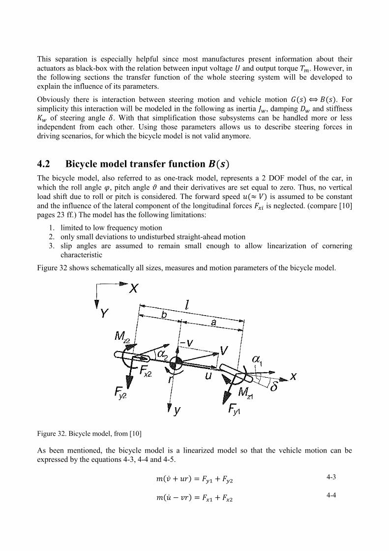
The bicycle model, also referred to as one-track model, represents a 2 DOF model of the car, in
which the roll angle , pitch angle and their derivatives are set equal to zero. Thus, no vertical
load shift due to roll or pitch is considered. The forward speed is assumed to be constant
and the influence of the lateral component of the longitudinal forces is neglected. (compare [10]
pages 23 ff.) The model has the following limitations:
1. limited to low frequency motion
2. only small deviations to undisturbed straight-ahead motion
3. slip angles are assumed to remain small enough to allow linearization of cornering
characteristic
Figure 32 shows schematically all sizes, measures and motion parameters of the bicycle model.
Figure 32. Bicycle model, from [10]
As been mentioned, the bicycle model is a linearized model so that the vehicle motion can be
expressed by the equations 4-3, 4-4 and 4-5.
4-3
4-4

CHALMERS, Applied Mechanics, Master’s Thesis 2013:45 40
4-5
4-6
4-7
The lateral forces in equation 4-3 and 4-5 are replaced by the expression 4-6, introducing cornering
stiffness and lateral wheel slip angles , leading to equation 4-8 and 4-9.
(4-6) and (4-3):
{
} 4-8
4-9
By elimination of velocity , one receives the second-order differential equation 4-10.
(4-8) and (4-9):
{ }
{
}
4-10
By introducing the terms 4-11 this can be further simplified to 4-12.
4-11
4-12
Accordingly, the linearized bicycle model is of the form (4-26) with parameter (4-32).
4-13
[
]
[
]
(
) [
]
⁄
⁄ 4-14
From there, the transfer function (4-15) with and for yaw rate can be directly
received. Transfer functions for and for are given by 4-16 and 4-17, whose
parameter , and are implemented more easily with a state-space model in Matlab.
4-15
4-16
4-17
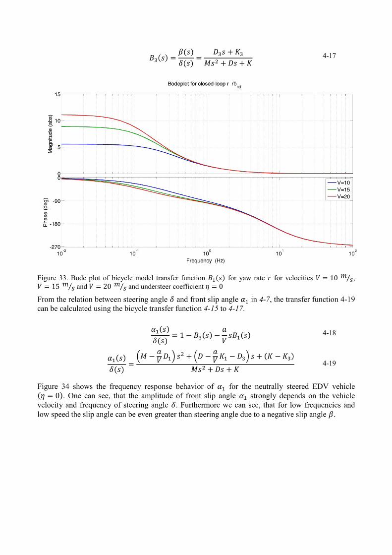
Figure 33. Bode plot of bicycle model transfer function for yaw rate for velocities ⁄ ,
⁄ and ⁄ and understeer coefficient
From the relation between steering angle and front slip angle in 4-7, the transfer function 4-19
can be calculated using the bicycle transfer function 4-15 to 4-17.
4-18
( ) (
)
4-19
Figure 34 shows the frequency response behavior of for the neutrally steered EDV vehicle . One can see, that the amplitude of front slip angle strongly depends on the vehicle
velocity and frequency of steering angle . Furthermore we can see, that for low frequencies and
low speed the slip angle can be even greater than steering angle due to a negative slip angle .

CHALMERS, Applied Mechanics, Master’s Thesis 2013:45 42
Figure 34. Bode plot for front slip angle transfer function ⁄
As mentioned previous, for simplicity we will handle vehicle motion and steering motion
independent from each other. Since we are interested in great slip angles between 1-2 Hz for
maximum tire forces, which are likely to occur at higher speeds, we can see from Figure 34 that it is
a good approximation to assume slip angle equals steer angle (4-20).
4-20
With that simplification we can describe the load torque of steering system as function of
inertia , damping and stiffness of steering angle .
4.3 Steering system transfer function
The equations 4-21 to 4-25 show the four basic equation of a DC motor for rotor mechanics (4-21),
electrical circuit (4-22), motor torque (4-23) and back EMF (4-22). Equations taken from [13].
4-21
4-22
4-23
4-24
4-25
The load torque in (4-26) is defined by inertia , damping and stiffness for turning the
wheels. The stiffness (4-27) is direct outcome of the detailed force analysis in chapter 3 with
torque stiffness as function of wheel load, pneumatic and mechanical trail.
⏟
4-26
[
] 4-27
1 [
] 4-28
2 [
] 4-29
One can show that damping (4-28) is more influenced by damping of the rack-and-pinion-
system, especially the bearings and knuckles. Thus, the influence of suspension geometry on
damping is negligible. The value is based on the assumption of a similar project with steer-by-wire
car performed at Stanford University [4]. This value is most likely to be smaller for the EDV due to
smaller tire and simpler steering system, so that with this assumption load torque will be
overestimated. Same applies for lumped inertia (4-29) of rack and wheels about the steering axis.
Since cornering stiffness is strictly speaking only valid for slip angles , we will define at
this point the cornering stiffness slightly different to calculate so that it builds up maximum
lateral tire force more precise (4-30). Otherwise maximum tire forces would be overestimated.
|
4-30
Rotor inertia and damping can be lumped together with load torque (4-31) with the constant relation
between rotor angle and wheel angle (4-32) so that we end up with a second-order equation for
the mechanical part of the steering system (4-33).
(
( ) )
⏟
(
( ) )
⏟
(
( ) )
⏟
4-31
4-32
4-33
Integrating mechanical circuit (4-33) and electrical circuit (4-22) in (4-34) and (4-35) we receive the
transfer function for rotor speed over voltage input for the actuator (4-36).
4-34
1 rack and tire damping about kingpin axis, value based on estimations made in [2], [15], [16], see also
section 4.5
2 rack and tire inertia about kingpin axis, value based on estimations made in [2], [15], [16], see also section
4.5
CHALMERS, Applied Mechanics, Master’s Thesis 2013:45 44
4-35
4-36
By integrating we receive the transfer function for rotor angle over DC motor voltage (4-38).
4-37
(
) (
) (
)
4-38
We can see that the transfer function for rotor speed (4-36) is of second order. Since we need to
control rotor angle to control the wheel angle a third-order transfer function is necessary
(4-38).
From equation 4-35 and 4-34 also the transfer function for DC motor current (4-39) and, hence,
the actuator output torque (4-40) can be calculated.
4-39
4-40
Since the rack-and-pinion system is set to be rigid and, hence, linear relation between rotor and
wheel angle can be assumed, the open-loop transfer function (4-42) is of third order.
4-41
( )
(
) (
) (
)
4-42
One has to design the systems parameter already in such a way, that the open-loop characteristic
doesn’t show too much phase lag (time lag). Equation 4-43 shows the phase equation of transfer
function . The poles of are given in 4-44, 4-45 and 4-46. The best way to guarantee stable
behavior is to increase their critical frequencies of the poles so that they don’t fall into the working
range in order to decrease phase lag.
[
]
4-43
4-44
4-45
4-46
Some parameters are fixed, so and can’t be influenced. But through the right choice for an actuator
the electro-dynamic parameter can be chosen and mechanical parameter of the steering system can
be influenced by steer ratio and gear ratio of the actuator.
4.4 Controller transfer function
The steering angle input from the driver is measured by a wheel angle sensor, whose output voltage
is nearly linear to steering wheel angle input . This output voltage is than amplified to control
the actor angle. Common sensors have a linear accuracy error of . The transfer function
cutoff frequency of the electric sensor is high compared to the mechanical transfer function so that a
linear behavior for relevant frequencies can be assumed (4-49).
4-47
4-48
4-49
The sensor transfer function is integrated into the controller transfer function (4-51) of a
simple PID-controller. The control parameter are optimized to guarantee stable response behavior
with low power requirements of the closed-loop (4-52).
4-50
( ) (
) 4-51
4-52

CHALMERS, Applied Mechanics, Master’s Thesis 2013:45 46
4.5 Control and steering system parameter
Table 10 shows the parameter, for which the steering system has been optimized. The last rows
show different aligning torque stiffness and corresponding cornering stiffness for different
suspension geometry setups, which results from the analysis in chapter 3.
Table 10. Steering system parameter [4] [3]
Symbol Description [unit] Value
steering ratio 11
gear ratio 5
inertia of rotor [ ⁄ ] 0.004
inertia of gear box about rotor shaft [ ] 0.000145
inertia of coupling shaft [ ] 0.002
lumped inertia of rotor, gear box and coupling shaft [ ] 0.0045
lumped inertia of steering rack and wheels about steering axis
[ ]
53
rotor damping ⁄ 0.0000035
rack and tire damping about steering axis ⁄ 2254
steering arm about kingpin axis [ ] 0.1
internal resistance of DC motor 1.2
actuator induction [ ] 9.5
DC motor moment constant 0.544
DC motor voltage constant 0.544
voltage amplification factor 47.4
sensor voltage constant 1
Controller proportional constant 15.41
Controller derivative constant 0.25
Controller integrative constant 31.08
tire-to-ground friction coefficient 1.5
Stiffness parameter for tire friction force
maximum aligning torque 6 25 63
aligning torque stiffness 229 448 634
cornering stiffness 45000 19000 12000
3 The assumption of inertia of the steering system for steering shaft, rack- and pinion-system and wheels is
based on estimations made in [4], [15] and [16]. In these papers control concepts for similar cars are
presented, such cars equipped with a steer-by-wire system or electric power assisted steering. One can see
that still for those similar concepts the estimations vary considerably. Since the EDV can be expected to
have a rather simple steering system the mean value of those presented has been taken from Li LIU [15].
The exact estimation of this value for the EDV is not possible at this point, since the steering system is not
designed yet. However, for precise steering control those parameter are crucial and it is advisable to identify
them experimentally when the EDV is set up.
4 For the damping of the steering system same estimations have been made as described above, based on
assumptions from [4], [15] and [16].

5 Results
5.1 Tire torque in relevant scenarios
The results of this work are strongly focussed on the tire friction torque prediction in relevant
driving scenarios. Hence, Table 11 to Table 13 show again the results of chapter 3, which focus on
the influence of suspension geometry – as function of caster trail and scrub radius - on the friction
force amplitude. Those results can be used for different suspension setups.
Table 11. Static torque prediction for
Table 12. Combined steering and braking kingpin moment
Table 13. Overall steering torque for vertical force impact
Setup 5 with in the tables above can be – from the current point of view –
assumed to describe the suspension setup of the EDV the closest. Generally, the suspension
geometry should be set up in such a way that scrub radius and caster trail are reduced as much as
possible. However, certain variations due to construction tolerances have to be taken into account.
During vertical wheel motion suspension geometry and parameters can change slightly. This can be
considered by assuming a certain variation of scrub radius and caster trail. Thus, from that
perspective setup 5 is also favorable and will be considered from now on in the following results
and discussion.
5.2 Actuator torque with steering control
The following results are restricted to one specific actuator setup only. The control system is
optimized for the actuator described in Table 10. The table lists all parameter used for the following
results. Especially the electro-dynamic power requirements can vary a lot depending on the chosen
steering actuator. The simulation has been accomplished for setup 5, as described in the previous
section.

CHALMERS, Applied Mechanics, Master’s Thesis 2013:45 48
Figure 35 shows the bode plot for the open-loop response in comparison with the controlled
closed-loop .
Figure 35. Bode plot for open-loop and closed-loop transfer function of
As been mentioned before, the open-loop of the steering system should already show good
frequency response behaviour to reduce the required compensation effort of the closed-loop.We can
see that the controller shifts the cut-off frequency to and reduces phase lag. The
frequency has been set as critical frequency for the EDV, which is expected to be the
maximum frequency of the driver input. For that frequency a phase lag of could be
achieved, which equals a time-lag of .
Figure 36 on the next page shows the frequency response of alignment torque for both wheels with
mechanical trail of . One can see that dynamic wheel torque due to damping has
considerable impact for frequencies .

Figure 36. Bode plot of self-alignment torque on both wheel for mechanical trail e=20 mm
The red line in Figure 36 shows the overall wheel torque. The green line shows wheel torque due to
damping and blue shows steering effort due to tire friction. We can see that the frequency response
for friction forces (blue) is in accordance with the numerical results given in Table 11, Table 12 and
Table 13. The friction torque in the closed-loop system decreases with increased frequency due to
decreased steering angle amplitude, since the actuator is not able anymore to follow the required
steering angle amplitude.
The plots on the following two pages show the time response behavior for the controlled system for
sinusoidal steering input and steering step input.
Figure 37 shows the time response to a sinusoidal steering input with amplitude of ., the
angle of maximum alignment torque for mechanical trail . As for a step response, in the
beginning rather high torque and power is necessary to react to steering input. The steady-state
requirements are lower than. The response behavior for small mechanical trail can be found in
APPENDIX E.
Figure 38 shows the time response on a steering angle step. The steering input is modeled not as an
ideal step, considering that the driver input will also take a certain amount of time to reach the final
step value. As been mentioned before, the steering angle step can be also understood as static torque
and jacking torque.

Figure 37. Time response for and

Figure 38. Time response behavior to steering step input ( for ) and rise time

Table 14 shows the evaluation of frequency and time domain analysis for different load case scenarios.
It lists the numerical results and the respective peak values estimated for each parameter.
Table 14. Power requirements: Evaluation of frequency and time response
Load case Torque
[Nm]
Rotor speed
[rpm] Voltage [V] Current [A] Power [W]
30 350 25 10 250
30 350 25 10 250
25 350 25 10 180
If we look now at the frequency response behavior of the vehicle for this specific setup and actuator in
Figure 39 we can see that the dynamics and time lag of the vehicle are not crucially affected by the use
of a steer-by-wire system. One could also think of some kind of second closed-loop with a yaw rate
sensor to improve steering response behavior in comparison to a conventional steered vehicle. The
yaw rate response in Figure 39 is based on the steering control behavior in Figure 35.
Figure 39. Frequency response behavior of vehicle yaw rate for closed-loop steering control
5.3 Actuator choosing
When searching for suitable actuators one can note fast, that actuators are often only given as “black-
box” system with voltage input and output torque and speed , as mentioned before.
Figure 40. Steer-by-wire control system with unknown actuator transfer function

In order to set power requirements we can set the requirement that the actual steering angle equals
the intended steering angle (5-1).
5-1
From there the turning velocity of the wheels (5-2) and its maximum (5-3) can be defined:
5-2
| |
| | 5-3
By using the steering ratio the output speed requirements of the actuator can be defined (5-4).
| | | |
⁄ 5-4
Table 15 shows the speed requirements for steering ratio of .
Table 15. Output speed requirements for actuator
Steer angle velocity Wheel turn speed[rad/s]
Wheel turn speed[deg/s]
Wheel turn speed [rpm]
Actuator speed [rpm] (rs=11)
Actuator speed[deg/s] (rs=11)
| | 0.55 31 5 55 330
| | 2.2 126 21 231 1386
| | 2.74 157 26 288 1728
Similar considerations can be made on load torque . The wheel torque is described by equation 5-5.
5-5
Using (5-1) for it can be rewritten to (5-6) with the maximum friction torque amplitude | |
for steering angle amplitudes (5-7).
5-6
| | 5-7
| | has been set to the maximum friction torque for the combined braking and steering case,
since maximum spin torque doesn’t fast turning speed and thus, the influence of
damping and inertia can be neglected. Lumped damping of the steering system about kingpin axis has
been set to ⁄ and lumped inertia to , as has been explained in
section 4.5.
From there, maximum wheel torque and maximum actuator load torque can be
evaluated. The results are given in Table 16 for sinusoidal driver input with different steering
amplitude and frequency.
Table 16. Output torque requirements for actuator
Load case Wheel Torque [Nm]
Actuator torque [Nm] (rs=25)
Actuator torque [Nm] (rs=16)
Actuator torque [Nm] (rs=11)
Steering rack force [N] (rst=10 mm)
| | 88 3.5 5.5 8 880
| | 128 5.1 8 12 500
| | 500 20 32 46 5000
| | 725 29 45 66 7250

CHALMERS, Applied Mechanics, Master’s Thesis 2013:45 54
In the previous section it could be shown that steering angle step response doesn’t show significant
torque amplitudes than the sinusoidal response for . Thus, the torque requirements in Table
16 can be seen as upper limits. We can see that for great steering angle amplitude and
low frequency wheel torque equals maximum spin torque amplitude.
For higher frequencies we can see the crucial impact of inertia and damping in the system. As been
mentioned before in section 4.5, the precise estimation of inertia and damping can be only
accomplished with the ready built EDV. It is recommendable then to identify those parameters
experimentally to improve steering control precision.
6 Conclusions
A great deal of importance in this work has been laid on the possibility of adaption of the results to
change of parameters. Since by the end of this thesis work the concept of the EDV hadn’t been
finalized yet, the transferability of results to change in design and components was of crucial
importance.
In order to produce trustable results in the analysis for sizing the steering actuator, limiting values in
the estimation of unknown parameter had been chosen. This has been accomplished by means of
suspension geometry, tire forces and steering dynamics.
The report focusses on the analysis of tire friction forces in relevant driving scenarios and the study of
the influence of suspension geometry on steering effort. This could be accomplished in an analytic
way. Particular focus in has been laid on the influence of caster trail and scrub radius on steering
effort. The final results are based on the estimation of and , which considers
already the change of suspension geometry due to vertical wheel motion.
Maximum tire forces have been estimated with respect to physical limitations of the tire. For that
purpose a friction coefficient of has been assumed throughout this work. This assumption
overestimates the actual maximum friction coefficient but serves as a sort of security margin, which
means it can be assumed that real tire forces won’t be larger than the given results.
Four relevant driving scenarios have been considered as actuator dimensioning driving scenarios, in
which maximum steering torque is expected. Those are:
1. Tire spin torque in parking conditions
2. Jacking torque due to high dynamic vertical wheel load
3. Self-aligning torque in high-speed cornering
4. Steering torque for combined braking and steering case during high-speed cornering.
The maximum steering torque due to tire friction of both wheels of the EDV has been identified as
for static spin torque.
Tire forces are results of vehicle dynamics. However, in the steering system they have been modelled
as static load as function of steering stiffness of steering angle about the kingpin axis. Dynamic
steering forces due to damping and inertia of the system, necessary to define the actual load torque of
the steering system, haven’t been analysed in this work, but estimated from reference works ([4], [14],
[15]).
For damping of steering rate the lumped damping coefficient about the
kingpin axis has been used. For the steering system’s inertia about the kingpin axis has been used. Those two parameters strongly depend on the components of the steering system,
such as steering rack and pinion, steering knuckles, tire types. Since they strongly influence the
amplitude of steering torque during fast steering motion, it is highly recommended to identify those
parameters experimentally for the finalized EDV.
Steering control analysis showed that electro-dynamics of the actuator are of particular importance and
analysing of the overall closed-loop response behaviour is necessary to guarantee sufficient control
time and precision.
However, this can be particular difficult, since a lot of manufacturers provide their actuators as black-
box systems only with information about input voltage and output torque or speed. For that reason
power requirements for the steering actuator have been in terms of dynamic load torque, which is a
function of steering angle frequency and amplitude, as well as steering ratio . The latter one can be
specifically used to adjust the steering system to the actuator characteristic. Since a steer-by-wire
CHALMERS, Applied Mechanics, Master’s Thesis 2013:45 56
doesn’t set requirements to steering ratio it can be set according to the needs, which means that it can
either used for decreasing the torque requirements or to increase the speed of steering motion.
With limits of steering angle amplitude | | , steer frequency and
steering ratio rough performance requirements for the steering actuator have been set to:
1. Actuator output torque
2. Actuator output speed
3. Actuator output power
As proposed in the beginning, the steer-by-wire system can be also accomplished by a setup with
linear steering actuator. In this case, the driver steer angle input is directly transferred into a linear
motion, which sets the wheel steering angle . For this setup the performance requirements can be set
to (assuming steering radius on upright ):
1. Actuator output force
2. Actuator output speed
3. Actuator output power
The estimation of energy demand for the actuator has not been done yet at this point since it strongly
depends on the final steering system design. For this purpose, it would be also necessary to develop a
standardized steering profile for city driving, high-way driving, etc. However, it can be stated at this
point, that one of the big advantages of electronic powered steering is, that it can be designed in such a
way, that energy is only required during steering motion. Energy for the steering system is not required
for [14].
June 2013

7 References
[1] E. Vijayakumar, ”Thesis work: Frame stiffness and mass estimation analysis for electric one-
seater prototype,” Volvo Group Truck Technology, Göteborg, Sweden, 2013.
[2] P. H. Winner, Fahrdynamik und Fahrkomfort, Darmstadt: FZD TU Darmstadt, 2011.
[3] N. D. Smith, ”Understanding Parameters Influencing Tire Modeling,” Colorado State University,
2004 Formula SAE Platform, 2004.
[4] P. Yih, "Steer-by-wire: Implications for vehicle handling and safety (Dissertation PhD)," Stanford
University, San Francisco, CA, Januar 2005.
[5] T. Rattfelt, ”Thesis work: Preparatory Component Selection for Design of Prototype Electric One-
Seater Car,” Volvo Group Truck Technology, Göteborg, 2013.
[6] DIN, ”DIN 70020-1,” DIN, Germany.
[7] Y. G. CHO, "Vehicle steering returnability with maximum steering angle at low speeds,"
International Journal of Automotive Technology, p. 431−439, Vol. 10, No. 4, 2009.
[8] G. Rill, ”First order tire dynamics,” i III. European Conference on Computational Mechanics,
Lisbon, Portugal, 2006.
[9] R. g. R.s. Sharp, "On car steering torques at parking speeds," Part D: Journal of Automobile
Engineering, pp. 87-96, 2003.
[10] H. B. Pacejka, Tyre and Vehicle Dynamics, Second Edition, Rotterdam: Butterworth-Heinemann,
Oxford, 2006.
[11] A. Tires, ”avonracing.com,” Avon Tires, [Online]. Available: http://www.avonracing.com. [Använd
04 2013].
[12] R. M. Brach, ”Modeling Combined Braking and Steering Tire Forces,” SAE TECHNICAL PAPER
SERIES, Vol. %1 av %22000-01-0357, 2000.
[13] P. D.-I. R.Nordmann, Mechatronische System im Maschinenbau I, Darmstadt, Germany: TU
Darmstadt, 2005.
[14] M. Mitschke, Dynamik der Kraftfahrzeuge, Band B, Schwingungen, Heidelberg: Springer Verlag
Heidelberg, 1984.
[15] M. N. P. R. Li LIU, ”On Torque Control of Vehicle Handling and Steering Feel for Avoidance
Maneuver with Electric Power Steering,” i 17th World Congress The International Federation of
Automatic Control, Seoul, Korea, 2008.
[16] B.-C. J. a. S.-C. L. Du-Yeol Pang, ”Steering Wheel Torque Control of Electric Power Steering by
PD-Control,” i KINTEX, Gyeonggi-Do, Korea, 2005.

CHALMERS, Applied Mechanics, Master’s Thesis 2013:45 58

APPENDIX A Vertical dynamics analysis
A standard model used in vertical dynamics is the Quarter-Car-
Model (Figure 41), which is given by a 2 DOF two-mass oscillator
representing the vertical model of a single wheel. In Figure 41 the
two masses are given by the unsprung mass , which is mainly
given by the wheel mass, and the sprung mass , the partial body
mass loaded on that wheel. and represented stiffness and
damping values of the tire and and those of the suspension.
The values and are values given by the type of tire chosen.
The vertical dynamics analysis using a quarter-car-model can be
used to get a first estimation for stiffness and damping adjustment
and of front and rear suspension. Purpose of the suspension
system is on the one hand to provide road holding at all time and on
the other hand to reduce vibrations on car and passenger coming
from the road. A 2 DOF system shows two critical Eigen
frequencies. Those are the frequencies, at which it comes to
resonance, meaning that the impact of road disturbance is the
greatest.
Figure 41. Quarter-Car-Model
7-1
Equation 7-1 shows the representation of the quarter-car-model. The sprung mass and the
unsprung mass are not completely separable. For example, the components of suspension are
partly sprung and unsprung. For precise definition of both masses, measurements would be necessary.
In most cases, counting half of the connection components (such as wishbones, A-arms, etc.) to sprung
and half of it to unsprung mass, is a good approximation.
7-2
7-3
7-4
Equation 7-4 and Figure 43 show a way to model the road input . As can be seen from Equation 7-3
and Figure 42, is the frequency of the road input a function of car velocity and wave length . We
can see that the road input frequency coincides with the critical Eigenfrequencies of wheel and
body at and for a car velocity of . Thus, the stiffness and damping
coefficient of the suspension have to be chosen such that they reduce the vertical movement and
acceleration at those critical frequencies. However, the stiffness value also affects the critical
Eigenfrequency of the body due to the relation given in equation 7-5.

CHALMERS, Applied Mechanics, Master’s Thesis 2013:45 60
√
7-5
Figure 42. Excitation frequency of road input , [2]
Figure 43. Road bump model [7]
One difficulty is given for road puts
with discontinuous characteristics,
such as an impulse or step. In this case,
the frequency input is almost
distributed over the whole range of
frequencies, which can cause
disastrous failure. Since an ideal
impulse doesn’t exist in reality, it will
always have certain continuity in the
excitation and only road inputs with
will be considered.
Nevertheless, it has been taken into
account that the frequencies of road
irregularities can spread over a wide
range of frequencies.
The assessment of the body acceleration and the wheel load gives good information about
ride comfort and endurance strength of the car. Figure 44 shows that an increase of the unsprung
mass lowers the second resonance frequency, but on the other side increases the wheel load
(and accelerations) and the frequency spectrum becomes wider [2].

Figure 44. Influence of the unsprung mass [14]
However, in Figure 45 it is possible to see that an increase of the body mass certainly affects
the first resonance, the body frequency, but also lowers body acceleration in the second
resonance, while the wheel load remains unchanged.
Figure 45. Influence of body mass [14]

CHALMERS, Applied Mechanics, Master’s Thesis 2013:45 62
Figure 46. Influence of body stiffness [14]
Since the body stiffness is connected to both, the sprung and the unsprung mass, it affects both
resonances, and an increase of the stiffness has positive effects on the wheel load, as can be seen
in Figure 46.
Figure 47. Influence of body damping [14]

Figure 47 shows that the body damping lowers the peaks of the resonances, whereas it has negative
effects on the overcritical regions.
The given graphs are showing that, when adjusting the parameters, a compromise between ride
comfort (weighted vibration intensity ) and driving safety (normalized wheel load fluctuation)
has to be found. This can be drawn in a conflict diagram (Figure 48), in which both criteria are laid on
top of each other. In one case the damping is changed while the stiffness is kept constant and the other
way around. There is a physical boundary curve, which can’t be undercut. In the adjustment progress
of the solar project the focus will be more on the driving safety than ride comfort. Nevertheless, it has
to be guaranteed that there will be no physical damage to the driver [14].
Figure 48. Conflict diagram suspension adjustment [2]

CHALMERS, Applied Mechanics, Master’s Thesis 2013:45 64
APPENDIX B Spin torque and relaxation length
Due to the elasticity of the tire, lateral forces will not directly build up, but take a certain time. G. Rill
[8] presents a model to describe those dynamics tire forces as a first-order system (3-1).
Figure 49. Lateral tire deflection [8]
With lateral stiffness and the lateral damping property of the tire the dynamic tire force can be
written as function of lateral deflection (7-9). Combined with 3-1 and 3-3 relaxation time constant
(7-11) can be derived and from there relaxation length (7-12). Those two sizes describe the time
and distance necessary until a change of slip conditions leads to a steady-state force amplitude as a
function of rotation speed of the wheel.
The force equilibrium in point Q in Figure 14. Lateral tire deflection is then given by
( )⏟
( )⏟
7-6
| |
7-7
| | 7-8
7-9
| | 7-10
(
| |)
⏟
7-11
| | | |
(
| |) | |
7-12
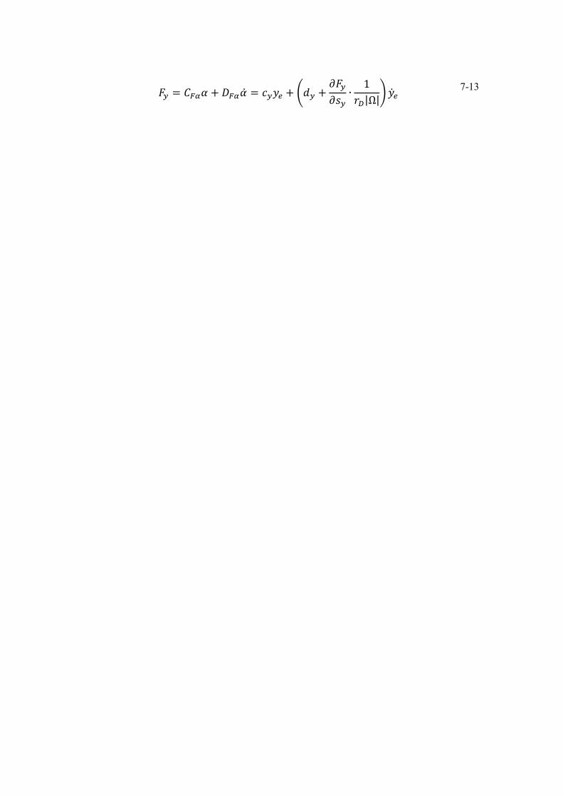
(
| |)
7-13
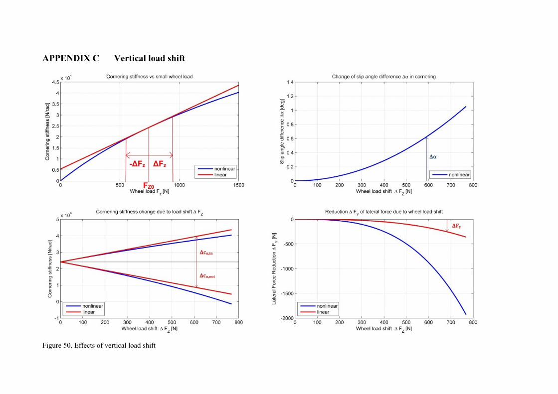
APPENDIX C Vertical load shift
Figure 50. Effects of vertical load shift

CHALMERS, Applied Mechanics, Master’s Thesis 2013:45 67
APPENDIX D Tire properties
Figure 51. Self-aligning torque vs. slip-angle, from [11]

CHALMERS, Applied Mechanics, Master’s Thesis 2013:45 68
APPENDIX E Steering control analysis
Figure 52. Time response for and

CHALMERS, Applied Mechanics, Master’s Thesis 2013:45 69
Figure 53. Time response for and

CHALMERS, Applied Mechanics, Master’s Thesis 2013:45 70
Figure 54. Time response behavior to steering step input and rise time
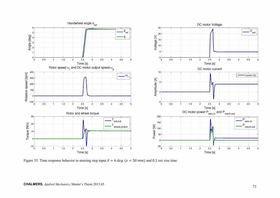
CHALMERS, Applied Mechanics, Master’s Thesis 2013:45 71
Figure 55. Time response behavior to steering step input and rise time

CHALMERS, Applied Mechanics, Master’s Thesis 2013:45 72