steam turbine thermal modeling for improved transient ...765657/fulltext01.pdf · la mejor mamá...

Steam Turbine Thermal Modeling for Improved Transient Operation

MONIKA TOPEL

Licentiate Thesis, 2014

KTH Royal Institute of Technology

Industrial Engineering and Management

Department of Energy Technology

Heat and Power Division

SE-100 44, Stockholm, Sweden

TRITA KRV Report 14/06

ISSN 1100-7990

ISRN KTH/KRV/14/06-SE

ISBN 978-91-7595-367-0

© Monika Topel, 2014

Akademisk avhandling som med tillstånd av KTH i Stockholm framlägges till offentlig

granskning för avläggande av teknisk licentiatexamen fredagen den 5 december kl. 11:00 i

sal Learning Theater (M235), KTH, Brinellvägen 68, Stockholm. Avhandlingen försvaras på

engelska.

Para Raquel,

La mejor mamá del mundo.

Abstract

The growing shares of renewable energy sources in the market and

solar thermal power applications have set higher requirements on steam

turbine operation. These requirements are related to flexibility during

transients. A key aspect sought of such flexibility is the capability for fast

starts. Due to the varying temperature gradients during start-up, the

speed at which the turbine can start is constrained by thermal stresses

and differential expansion. These phenomena either consume component

lifetime or may result in machine failure if not carefully controlled.

In order to accomplish faster starts while ensuring that lifing

requirements are preserved, it is important to analyze the thermal

behavior of the machine. For this, a transient thermal model was

developed with a focus on adaptability to different turbine sizes and

geometries. The model allows for simple and fast prediction of thermo-

mechanical properties within the turbine metal, more importantly, of the

temperature distribution and the associated thermal expansion.

The next step of this work was to validate the assumptions and

simplifications of the model. This was done through the study and

comparison of two turbines against measured operational data from their

respective power plants. Furthermore, validation studies also included

comparisons concerning the geometric detail level of the model. Overall,

comparison results showed a large degree of agreement with respect to

the measured data and between the geometric detail levels.

The validated model was then implemented in studies related to

reducing start-up times and peak differential expansion. For this, the

potential effects of turbine temperature maintaining modifications were

investigated and quantified. The modifications studied included:

increasing gland steam pressure, increasing back pressure and increasing

barring speed. Results yielded significant improvements starting from

9.5% in the start-up times and 7% in the differential expansion.

Keywords

steam turbines, transients, start-up, finite element model, heat transfer.

Sammanfattning

En växande andel förnyelsebara energikällor samt tillämpningar med

termisk solenergi har ökat kraven på ångturbindrift. Dessa krav är kopplade

till flexibilitet under transienter. En eftersträvad nyckelparameter för ökad

flexibilitet är snabba uppstarter. På grund av varierande

temperaturgradienter under uppstartsprocessen är den nödvändiga tiden för

att starta turbinen begränsad av termiska spänningar och ojämn termisk

expansion. Dessa fenomen förbrukar antingen komponenters livslängd eller

kan leda till haveri om de inte är noga kontrollerade.

För att åstadkomma snabbare starter samtidigt som underhållsintervaller

bevaras är det av stor betydelse att analysera den termiska karakteristiken

hos maskinen. För detta utvecklades en transient termisk modell med fokus

på anpassningsbarhet till olika turbinstorlekar och geometrier. Modellen

möjliggör enkel och snabb beräkning av termo-mekaniska egenskaper i

konstruktionsmaterialet samt den ännu viktigare temperaturfördelningen

och tillhörande termiska expansionen.

Nästföljande steg i arbetet var att validera de antaganden och förenklingar

som gjorts i modellen. Detta gjordes i form av en studie och jämförelse med

två turbinmodeller mot uppmätt driftdata från respektive kraftverken.

Dessutom inkluderades även en jämförelse av den geometriska

detaljrikedomen i valideringen av modellen. Sammantaget visade jämförelsen

god överenstämmelse med mätdata samt mellan de olika nivåerna av

geometrisk detaljrikedom.

Den validerade modellen implementerades sedan i studier relaterade till

att reducera uppstartstiden och högsta expansionsdifferens. För detta

undersöktes och kvantifierades potentiella effekter av modifikationer för att

bibehålla turbintemperaturen. Dessa modifikationer innefattade: höjning av

tycket för tätningsånga, höjning av utloppstrycket, samt höjning av

baxvarvtal. Resultaten gav betydande förbättringar, från 9.5% i uppstartstid

och 7% i expansionsdifferens.

Nyckelord

ångturbiner, transienter, uppstart, finitelement, värmeöverföring.

Preface

This thesis was completed at the Heat and Power Technology (HPT)

Division at KTH Royal Institute of Technology under the supervision of

Associate Professor Björn Laumert. Research at HPT is focused in the

fields of poly-generation, aeroelasticity, turbomachinery, biofuels in gas

turbine cycles and concentrating solar power.

This thesis addresses the thermal modeling of steam turbines. The

main motivation of such modeling is to be able to accurately predict

thermal behavior of turbines during transient operation. The outcomes of

this research serve as a basis for optimizing the nowadays more variable

operation of fielded turbines, especially those in concentrating solar

power plants.

The research has been funded by the Swedish Energy Agency, Siemens

Industrial Turbomachinery AB, GKN Aerospace and Royal Institute of

Technology through the Swedish research program TURBO POWER, the

support of which is gratefully appreciated.

Stockholm, December 2014

Monika Topel

List of appended papers

This licentiate thesis is based upon the following three scientific

articles:

Paper A

M. Topel, J. Spelling, M. Jöcker and B. Laumert (2014) “Geometric

Modularity in the Thermal Modeling of Solar Steam Turbines”, Energy

Procedia, Volume 49, Pages 1737-1746.

Paper B

M. Topel, M. Genrup, M. Jöcker, J. Spelling and B. Laumert (2015)

“Operational Improvements for Start-up Time Reduction in Solar Steam

Turbines”, Engineering for Gas Turbines and Power, Vol. 137(4).

Paper C

M. Topel, M. Jöcker, S. Paul and B. Laumert “Differential Expansion

Sensitivity Studies during Steam Turbine Start-up”, GT2015-42214,

Proceedings of the ASME Turbo Expo, Montréal, Canada, June 2015,

(draft under review).

Acknowledgements

I would like to thank Björn Laumert for being an amazing supervisor

and for giving me priceless guidance and encouragement. I would also

like to thank my co-supervisors Markus Jöcker and Magnus Genrup, for

their valuable input, feedback and countless answers to my questions.

Thanks also to Torsten Fransson for the opportunity to come to KTH.

Furthermore, I would like to thank the TURBOPOWER program for

their financial support of this work. In this regard, thanks to James

Spelling, for creating such a firm base from which I was able to learn and

use as a guide of my work.

Thanks to my colleagues in the Energy Department for creating a great

atmosphere that makes it easy to come to work every day and fun to join

in the occasional after-work. Special thanks to Jens Fridh, Nenad Glodic,

Petra Rytterholm, Torsten Strand, Wujun Wang and Maria Xylia.

My deepest thanks to those who have redefined the meaning of the

word “colleague” into: individual with which you have established a

friendship by means of a shared workplace; this concerns: Lukas

Aichmayer, Johan Dahlqvist, Florian Fruth, Tobias Gezork, Mauricio

Gutierrez, Lucio Monaco, Patricia Monzó, Johannes Morfeldt, Ranjan

Saha, Antonio Sanz, James Spelling and Manuel Welsch. I’m really

thankful for having you as “colleagues” and for the inspiration you have

provided through all the fun moments shared.

I would like to thank my friends outside of work for unknowingly

encouraging me through laughter and timely distractions, especially

Veluska Arias, Francisco Viña and Pedro Hernandez. Also thanks to the

Venezuelan crew for bringing a piece of home to Sweden. I’m also grateful

to Sara Aniyar and Karl-Göran Mäler for being so exceptional and for

treating me like one of their own.

I want to thank my family for their unconditional support and good

examples. This includes Gabriela Lucani and Rafael Guédez, whom I

consider to be my siblings. My endless gratitude goes to Mercedes Parra

for her motherly love and patience. Finally, I want to thank Raquel Topel,

to you I owe everything I am and everything I want to become.

Nomenclature

Abbreviations

BC Boundary Condition

CD Cool-Down

CSP Concentrating Solar Power

CSPP Concentrating Solar Power Plant

FE Finite Element

HPT High Pressure

HTC Heat Transfer Coefficient

LCF Low Cycle Fatigue

LPT Low Pressure Turbine

LSB Last Stage Blade

Latin Symbols

𝑐𝜃 Tangential flow velocity [m/s] 𝐶𝑝 Specific heat capacity [kJ/(kg K)]

𝐶𝑠𝑒𝑎𝑙 Labyrinth seal constant [m2] 𝐶 Aspect Coefficient [ - ] 𝑑 Diameter [m] 𝐸 Young modulus [Pa] 𝑒𝑖𝑛𝑠 Insulation thickness [mm] ℎ0 Total enthalpy [kJ/kg] ℎ1,2 Static enthalpy [kJ/kg]

ℎ𝑠 Isentropic static enthalpy [kJ/kg] 𝐻 Height of expansion chamber [mm] 𝐻𝑇𝐶 Heat transfer coefficient [W/(kg m2)] 𝑘 Thermal conductivity [ - ] 𝐾 Empirical correction factor [ - ] 𝑙 Length [m] �̇� Live steam mass flow [kg/s] �̇�𝑙𝑒𝑎𝑘 Gland steam mass flow [kg/s] 𝑁 Rotational speed [rpm] 𝑁𝑢 Nusselt number [ - ]

𝑃 Pressure [bar] 𝑃𝑟 Prandtl number [ - ] 𝑟 Radius [m] 𝑅𝑒 Reynolds number [ - ] 𝑅𝑒𝑢 Rotational Reynolds number [ - ] 𝑠 Disc gap [m] 𝑇 Temperature [oC] 𝑡 Time [s] 𝑢 Tangential velocity [m/s] 𝑣 Specific volume [m3/kg] 𝑊 Work [W] 𝑧 Number of teeth [ - ]

Greek Symbols

𝛽2 Blade outlet angle [ o ] 𝛽𝑚 Linear expansion coefficient [1/oC] 𝛿 Labyrinth radial clearance [mm] 휀 Volumetric gap fraction [ - ] 𝜂𝑠 Isentropic efficiency [ - ] 𝜆 Tooth width [m] 𝜇 Flow amount factor [ - ] υ Traverse expansion coefficient [ - ] 𝜌 Density [kg/m3] 𝜎 Stress [Pa] 𝜏 Tooth pitch [m]

𝜙 Mass flow coefficient [s C /m3]

Subscripts

𝑑 Disc

𝑓𝑟 Friction

𝑁𝐶 Natural Convection

𝑠 Seal

𝑣𝑡 Ventilation

Contents

1. Introduction ............................................................................. 1 1.1. Objectives .............................................................................................. 2 1.2. Methodology ......................................................................................... 4 1.3. Structure ................................................................................................ 5

2. Steam Turbine Fundamentals ................................................. 6 2.1. Thermal Processes ............................................................................... 7 2.1.1. Steam Expansion ...................................................................................... 7 2.1.2. Gland Steam Sealing ................................................................................ 9 2.1.3. Friction and Fanning ............................................................................... 10

2.2. Flexibility Demands ............................................................................ 12 2.2.1. Power Generation Mix............................................................................. 12 2.2.2. Concentrating Solar Power ..................................................................... 13

2.3. Turbine Transients and Cyclic Operation ........................................ 15 2.3.1. Thermal Stress and Fatigue .................................................................... 16 2.3.2. Differential Expansion ............................................................................. 17 2.3.3. Start-up Curves ....................................................................................... 18

3. Steam Turbine Transient Thermal Model ............................. 19 3.1. Steam Expansion Model .................................................................... 21 3.2. Gland Steam Sealing Model ............................................................... 22 3.3. Heat Conduction Model ...................................................................... 23 3.3.1. Geometric Modeling Approach ................................................................ 24 3.3.2. Boundary Conditions ............................................................................... 25

4. Results ................................................................................... 30 4.1. Model Validation ................................................................................. 30 4.1.1. Solar Steam Turbine ............................................................................... 30 4.1.2. Industrial High Pressure Turbine ............................................................. 35

4.2. Model Implementation ........................................................................ 43 4.2.1. Start-up Time Reduction ......................................................................... 44 4.2.2. Differential Expansion Reduction ............................................................ 54

5. Conclusions ........................................................................... 58 5.1. Future Work ......................................................................................... 59

References ................................................................................. 61

INTRODUCTION | 1

1. Introduction

In general, steam turbines are complex machines in which a wide

range of multidisciplinary mechanisms interact. The fundamental

working principle of steam turbines is comprised in the expansion of the

incoming steam, as it is through this expansion and using impulse to

generate shaft power that the energy conversion from heat to electricity

occurs. In addition, other relevant thermal processes within a steam

turbine are those of gland steam sealing and losses due to friction and

fanning.

Future scenarios of the primary energy mix for 2050 expect that fossil

fuels will remain a dominant source but that growth rates will be highest

for renewable energy sources with increases in the global share of 5-10%

[1]. The increased penetration of renewables in the grid implies that the

operation of steam turbines is required to be more flexible. The

requirements are mainly related to fast cycling capabilities for frequency

control as well as flexibility for start-up and shut-down.

Furthermore, the deployment of renewable technologies based on

steam cycles also poses higher requirements on steam turbine flexibility

during start-up. An example of this is the operation of steam turbines in

concentrating solar power plants (CSPPs). Due to the fluctuating nature

of the solar supply, the number of start-up cycles endured by solar steam

turbines is greater than those in base load plants [2], with multiple starts

possible during a 24h period.

The aforementioned requirements on steam turbine operation are

related to flexibility during transient operation, especially during start-

up. A key aspect sought of such flexibility is the capability for fast starts.

There are two main types of operating conditions a turbine can be subject

to: steady state and transient. The latter occurs when the conditions

under which the turbine is operating are variable. The most intrinsic

transient condition of a turbine is the start-up phase [3]. This is due to

the fact that start-up conditions are characterized by high thermal stress

states which compromise the lifetime of the turbine [4]. In addition,

differential thermal expansion is another phenomenon of concern during

2 | INTRODUCTION

start-up. If not carefully controlled, axial rubbing may occur between the

moving and stationary parts of the turbine, resulting in machine failure.

To avoid excessive thermal stresses during start-up, the manufacturer

may specify start-up curves which limit the rate at which the turbines can

reach full load. The purpose of the curves is to maintain thermal stresses

under a given temperature dependent limit [5]. The start-up time of a

turbine is determined by the permissible initial temperature step and the

subsequently permissible temperature transient [6]. What this translates

to is that, as a general rule, the warmer a turbine is before start the faster

the startup can be [3].

In order to accomplish faster startup speeds while still ensuring safe

operation of the turbine it is important to understand the thermal

characteristics of the machine. As thermal stresses and start-up curves

are temperature dependent, accurate prediction of the temperature

gradients within the steam turbines is thus necessary to be able to

optimize the operation of existing steam turbines, as well as improve the

flexibility of the next generation of turbines. It is therefore very important

to develop tools that can predict and give insight on the induced

temperature gradients.

Models for thermal analysis of steam turbines have been developed

and implemented in other works [7][8][9]. Similarly, previous work

performed at the Division of Heat and Power Technology at KTH also

focused on the development of a model for the overall prediction of

temperature distributions within the turbine [10].

One of these models consisted of a mixed 2D-3D FE approach

calibrated with transient temperature measurements of the steam path

[7]. In this model the numerical modeling scheme was directly dependent

on instrumenting the studied turbine, something that is not always

plausible and not generally applicable. The other model consisted of a 3D

FE approach using empirical correlations for the heat transfer zones [9].

However, the different turbine components were developed under large

computational dimensionality and they had to be considered separately.

By doing this, component interactions were not fully captured in

accordance with physical assumptions. The model developed previously

within KTH consisted of a full 2D axisymmetric that comprised the

interaction of all turbine components. However, this model was

developed for a single turbine without considerations of adaptability to

other turbines for future studies. Other drawbacks of the model were

INTRODUCTION | 3

related to the level of detail of the implemented boundary conditions and

the calibration of the heat transfer coefficients with the use of correction

factors.

In this work, the KTH thermal turbine model has been taken as a

reference for developing an improved modeling tool. The previous model

has been modified and refined in terms of geometric adaptability and

heat transfer assumptions. Similar to the preceding model, the newly

developed modeling tool consists of an integrated approach of steam and

heat transfer calculations performed on a full 2D axisymmetric turbine

geometry. However, the integration of a modular geometric modeling

approach allows the new model to be adaptable to various turbines.

Furthermore, other important changes consisted of including more

accurate heat transfer correlations and refining the implementation of the

boundary conditions to the model with respect to the mode of operation

of the turbine. These modifications were done with the focus of delivering

a fast calculating tool of sufficient level of detail to capture turbine

transient behavior.

Also in this work, the general applicability and accuracy of the model

have been evaluated in validation studies. The validation was performed

differently than the previous study from KTH as the heat transfer

coefficients were not corrected with weighting factors. Instead, the

developed modeling scheme was implemented in two different turbine

models while maintaining the same approach and assumptions. Finally,

the validated model has been implemented in parametric studies related

to steam turbine start-up improvements. The improvements were

obtained through the implementation of operational modifications

different from those studied previously [11].

1.1. Objectives

This thesis has two main objectives:

Establish a validated and efficient modeling tool which can accurately

predict the thermal behavior of steam turbines during transient

operation while being generally applicable in terms of heat transfer and

adaptable in terms of geometry.

Implement this tool in parametric studies concerning improvements

of the thermal response of steam turbines during start-up.

4 | INTRODUCTION

Furthermore, there is also an alternate, but not less important,

objective which comprises the fact that this thesis is meant to represent a

stepping stone for further research in the field of steam turbine

optimization for the flexible power plant operation.

1.2. Methodology

In order to achieve the aforementioned objectives, the method of

investigation that was carried out consisted of three steps, namely:

development, validation and implementation of the model.

The development of the modeling tool was done with the scope of

achieving sufficient level of detail of the turbine while keeping fast

calculation times. This was achieved with a 2D axisymmetric heat

conduction model with heat transfer coefficients (HTCs) based on

empirical heat transfer correlations. In general, the modeling scheme was

based in previous work performed at KTH. However, several changes and

improvements were performed to that model. One of main change was to

supplement the existing model with a COMSOL-based finite element (FE)

heat conduction model. Integration of COMSOL allowed for more

flexibility, including multi-physics applications. In parallel, the model

was also made more flexible with respect to the geometric modeling

approach. The previous model was tied to one specific turbine geometry,

and was thus cumbersome to use for the evaluation of alternative

turbines. Other very important changes consisted of including other

relevant heat transfer correlations and refining the boundary conditions

(BCs) implementation to the model with respect to the mode of operation

of the turbine.

The range of applicability and accuracy of the model was then

evaluated in the validation process. The validation focused on two main

aspects of the model: the geometric simplifications and the BC

assumptions. In order to validate these, comparisons were made against

measured operational data and other numerical models of higher

geometric dimensions. The former served to understand the range of

applicability of the BCs while the latter helped in the understanding of the

impact of the geometric simplifications.

Once having validated the model, the next step was to implement the

model. Parametric studies were carried out in order to investigate the

impact of three temperature maintaining modifications in the thermal

behavior of the turbine during transients. The studies were focused on

INTRODUCTION | 5

improving turbine response during start-up conditions. This was

analyzed calculating reductions on start-up time and differential

expansion.

1.3. Structure

This thesis begins with a first introductory chapter, in which the

background, the objectives and the method of investigation are presented.

Chapter 2 consists of explaining the fundamentals of steam turbine

technology which are relevant to the work performed in subsequent

chapters. Chapter 3 elaborates on the modeling approach developed to

simulate the transient thermal behavior of steam turbines. Chapter 4

presents the obtained results for the validation of the model and its

implementation in studies for the improvement of steam turbine

operational flexibility. Finally, Chapter 5 concludes the work in this thesis

and describes future work to be performed.

6 | STEAM TURBINE FUNDAMENTALS

2. Steam Turbine Fundamentals

Turbomachines are classified as all those devices in which energy is

transferred either to, or from, a continuously flowing fluid [12]. This is

performed by the dynamic action of one or more rotating blade rows

which change the swirl momentum of the working fluid (steam). Steam

turbines are one of the several kinds of existing turbomachines.

Essentially, steam turbines convert the thermal energy of high-pressure,

high-temperature steam into shaft work which then serves to drive a

generator or another determined process.

The operation of this machine is directly associated to the Rankine

cycle developed in the 19th century. The first steam turbines are attributed

to de Laval and Parsons in 1883 and 1884, respectively. As the century

passed, many people recognized the potential of the steam turbine and

dedicated development efforts to its improvement. Some relevant names

in this regard are: Rateau (1896), Curtis (1900), Ljungström (1912) and

Westinghouse (1897). In parallel, Stodola (1903) laid the foundation for

the theory behind of these machines.

Nowadays, steam turbines come in a variety of sizes and are widely

implemented as driving machines in ship transportation, industry and

power generation. Steam turbines are the dominant technology for

producing electricity worldwide [13]. This is related to the fact that

thermal energy is the most commonly used source of energy for electricity

generation globally, and has a greater installed capacity than any other

source of energy [14].

Unlike gas turbine systems where heat is a byproduct of power

generation, steam turbines normally generate electricity as a byproduct of

heat (steam) generation [15]. A steam turbine is dependent on a heat

source which is separate from the machine itself. This separation of

functions decouples steam turbines from only using fossil-based fuels,

allowing steam turbines to operate with a variety of fuels and heat

sources. For this reason, steam turbines are used in a wide range of power

generating conventional and non-conventional applications such as: oil,

gas, coal, biomass, geothermal, nuclear, solar and combined cycles.

STEAM TURBINE FUNDAMENTALS | 7

2.1. Thermal Processes

In general, steam turbines are complex machines in which a wide

range of multidisciplinary mechanisms interact. This section highlights

only the processes which are of importance and more relevance to the

work performed in subsequent chapters in relation to the modeling

approach.

2.1.1. Steam Expansion

The fundamental working principle of steam turbines is comprised in

the expansion of the incoming steam, as it is through this thermal process

that the energy conversion from heat to electricity occurs. This energy

transformation occurs within a turbine stage, which is composed of a

static blade row, denoted as stator, and a rotating blade row, denoted as

rotor. Essentially, the internal energy of the steam is transformed into

kinetic energy, and the latter in turn is transformed into mechanical work

that rotates the turbine shaft [16].

This process is synthesized by Euler’s turbomachine equation (1) in

which a change in total enthalpy ℎ0 is equivalent to a change in

tangential flow speed 𝑐𝜃 and/or rotational engine speed 𝑢. One key aspect

to equation (1) is the deviation of the flow produced by the shape of the

turbine blades. This flow deviation generates the tangential flow speed,

which in turn is the one velocity component in the direction of work-

producing forces.

The thermodynamic state and velocity conditions of the flowing steam

are directly related. Therefore, as the flow velocities change throughout

the stator and the rotor, so do the thermodynamic properties of the

steam. In general, as the steam expands its enthalpy and pressure

decrease. Figure 1 shows the enthalpy-entropy diagram of steam

expanding from state 1 to state 2. Furthermore, also represented in this

figure, are the stagnation states denoted with and the isentropic states

denoted with 𝑠. The efficiency of an expansion process is the ratio of the

real enthalpy drop to the isentropic enthalpy drop, shown in equation (2).

outoutinin cucuh ,,0 (1)


Figure 1 Turbine expansion process [12].

Steam turbines are commonly arranged in a multi-stage design, in

which each stage is an elementary turbine. Multi-stage configurations

make it possible to have steam extractions along the flow passage that

serve to increase the efficiency of the Rankine cycle through regeneration.

The amount of extracted steam and the inlet conditions to the turbine are

defined in the steady-state nominal design of the power plant.

Analogously, the steam expansion for the multi-stage turbine is defined

based on this given operating design point.

Under variable operating conditions, the steam expansion process

diverges from design. Pressure-flow relations in a multistage turbine in

off-design operation are complex phenomena [17]. One method for

calculating the highly nonlinear dependence of extraction pressures with

a flow is Stodola’s cone law. This law relates the inlet and outlet pressures

with the mass flow through the turbine by declaring that each turbine

section has a constant pressure ratio. Furthermore, it states that if the

pressure after a certain stage group varies in proportion to the steam

amount, the pressure values in all the previous stages vary in proportion

to the steam amount too [16]. This statement implies that the pressures in

the turbine are determined from the backpressure. The law is applicable

to intermediate turbine sections with constant mass flows as well as for

s

shh

hh

21

21

(2)


the whole multistage turbine. In this work, the law was implemented in

the modeling process and is explained with more detail in §3.1.

2.1.2. Gland Steam Sealing

Sealing glands are located at each end of the shaft, and fulfill two

functions: preventing the leakage of steam and avoiding the ingress of air

through the clearances between the rotating and stationary parts of the

turbine [13]. This has a pronounced effect on the overall efficiency of the

power cycle [18] and is achieved using of labyrinth-type seals which

restrict and minimize the fluid flow to or from the outside. The sealing

system has two modes of operation, which depend on whether the turbine

is highly loaded or in low load to stand-by mode. Figure 2 displays a

labyrinth joint geometry.

Figure 2 Steam turbine rotor showing labyrinth joints and steam flow paths through the labyrinth seals during (a) turbine operation and (b) stand-still.

During stand-by, the gland steam is entirely supplied from an external

source (Figure 2b). The external gland steam is injected into the labyrinth

joints in order to maintain the turbine sealed from the ingress of external

air [13]. Due to the vacuum conditions in the condenser, the low-pressure

side of the low pressure turbine is provided with external gland steam

even during normal turbine operation. Each end of the shaft is subject to

different temperature conditions. Therefore, the external gland steam is

provided at two different temperature levels to match those in the metal

surface and avoid inducing thermal stresses in the shaft.

As the turbine load increases, the steam in the labyrinths becomes a

mixture of external supply and internal leakages. Eventually, as the


turbine load reaches a certain level, the sealing is self-sustained from the

internal leakages of live steam to the seal [6] (Figure 2a). The load level at

which this occurs varies for each turbine type. However, typical values are

in the range of 40-60% load.

Steam expansion in a labyrinth seal is described by the process of

throttling [16], in which the pressure of the steam is decreased while

keeping the same enthalpy level. In addition, the nature of the flow

through the seal as the steam passes under each constriction is described

by a Fanno line [19], in which the leaked mass flow is dependent on the

inlet conditions of steam, the outlet pressure and the seal constant, as

shown in Equation (3). The seal constant can be expressed as a function

of geometric parameters such as the seal diameter 𝑑𝑠, clearance 𝛿,

number of teeth 𝑧, tooth pitch 𝜏 and tooth width 𝜆, see Equation (4).

2.1.3. Friction and Fanning

Among the external efficiency losses that occur in a turbine stage,

there are losses due to friction and ventilation. These take place in the

blades and discs of the turbine. As a turbine disc rotates in space,

aerodynamic resistance forces from the surrounding fluid act upon it [19].

In the gaps between the rotor and stator discs, recirculating steam flow

creates friction with the moving disc surfaces (Figure 3a). The energy

dissipated due to friction is proportional to the steam density 𝜌, the

square of the disc diameter 𝑑 and the cube of the circular speed 𝑢 and as

shown in Equation (5) [16].In addition, friction work is also dependent on

an empirical friction factor 𝐾 which is defined by geometric parameters

of the disc and the rotational Reynolds number, Equation (6).

2

1

out

in

in

insealleak

P

P

v

PCm (3)

z

zKdC sss

seal

),(),,( (4)


Similarly to friction, ventilation work is also proportional to density,

the cube of the circular speed and a blade aspect coefficient, as shown in

Equations (7) and (8) [20]. However, this energy dissipation, also known

as windage, occurs in the blade passages of the turbine instead of the

discs. The ventilation phenomenon is generally associated with partial

steam admission and low load at rear stage turbine operation. When the

turbine is partially loaded, a group of blade passages along the

circumference of the disc will be filled with stagnant steam. Owing to the

rotation of the disc, the steam filling these passages is subject to

centrifugal forces and moves from the roots to the tips of moving blades

[19]. The appearance of a vortex zone across the blade produces an

increase in steam and blade metal temperatures (Figure 3b) [16].This

effect is a characteristic of the last stage blade (LSB) of a turbine given the

dependency of Equation (7) on blade length. Note that this relation is

only valid in case of low volumetric flow through the steam turbine

blading.

Figure 3 Steam flow paths in the discs and blades of the turbine for (a) friction and (b) ventilation. [19]

23

2

1dfrfr duKW (5)

5/110/12 Re2105.2

udfr dsK (6)


2.2. Flexibility Demands

2.2.1. Power Generation Mix

World energy use increased more than ten times over the 20th Century

[21], and is expected to increase by between 27% and 61% by 2050 [22].

The main current conflict with the sustainability of energy supply is that

it is mostly derived from fossil fuels, which are not being newly formed at

the same rate as they are being consumed. Consequently, on one side,

there is a need to develop more efficient ways of using our current

sources. While on the other side, it becomes essential to explore and

expand the supply from sustainable renewable energy technologies.

The global energy scenario is tied to aspects of technological, societal,

environmental, governmental and economic nature. Due to this wide

range, when considering changes in the energy sector there is a trilemma

[22] that needs to be addressed. This trilemma consists of achieving

environmental sustainability, energy security and energy equity.

When considering future energy scenarios it is expected that fossil

fuels will remain dominant up to 2050. However, growth rates will be

highest for renewable energy sources with increases in the global share of

5-10% [1]. A direct consequence of these predictions is that the growing

shares of renewable energy sources in the market pose new challenges in

grid integration [23]. The main challenge is related to maintaining grid

reliability despite the intermittency of technologies such as wind and

solar PV. This variability directly affects the operation of conventional

power generating systems as it is required that they quickly respond to

such induced changes.

Although steam cycle generators haven’t been the predominant fast-

responding technology implemented to provide ancillary services, they

will be increasingly affected by the higher penetration of renewable

dbladevt dluCW 3 (7)

2sin58.0045.0 dblade dlC (8)


energy technologies. As such, steam turbine operation is required to be

more flexible [24][25]. The requirements are mainly related to fast

cycling capabilities for frequency control as well as flexibility for start-up

and shut-down. The latter requirement of start-up flexibility is not only

related to the variability of supply imposed by renewable technologies. It

also has to do with the search for competitiveness with peaking strategies

in liberalized electricity markets in which renewable technologies are

prioritized before others, therefore changing the role in supply of

equipment initially designed for base-load operation.

2.2.2. Concentrating Solar Power

Another aspect in which steam turbine equipment are being required

to be more flexible is in their utilization in emerging technologies. Such is

the case of concentrating solar power (CSP) in which the variability of the

solar resource is transferred to the operation of the turbine. CSP

technologies can be described with two energy conversion processes. The

first and foremost, since it is the one which includes the renewable part of

the technology, consists of collecting the solar direct irradiation and

converting it into heat. Then, this thermal energy can be either converted

into electricity by driving a heat engine or simply stored in the form of

heat for later use.

Solar radiation concentration is necessary in order to increase the

temperature of the heat collected from the sun. Concentration is achieved

through the use of a field of mirrors that collect the incident radiation and

reflect it to a receiver. The key for radiation concentration relies on

increasing the energy flux density from collector to receiver by reduction

of surface area. By concentrating the same amount of energy into a

smaller area, a larger quantity of useful thermal energy is obtained. It is

desirable to achieve high energy concentrations as this improves the

thermal efficiency of the whole system in accordance to Carnot.

In order to collect as much of the incident solar radiation as possible,

the collectors must track the sun’s position throughout the day. In

general, tracking mechanisms follow the sun with either a one or two-axis

movement, depending on whether the type of concentration is linear or

point focus, respectively. The two configurations currently used

commercially which comprise line focusing devices are: parabolic trough

(Figure 4a) and linear Fresnel reflectors (Figure 4b). Analogously, the two


commercially used configurations which comprise point focusing devices

are parabolic dish (Figure 4c) and central tower systems (Figure 4d).

The heat within the receiver is absorbed by a heat transfer fluid. This

heat is then exchanged to whichever working fluid is used by the heat

engine and thereby generating power in the power block. Nowadays, over

90% of all installed CSPPs are based on the use of Rankine cycles [26], in

which the power is generated by a conventional steam turbine. Due to the

fluctuating nature of the solar supply, the number of start-up cycles

endured by solar steam turbines is greater than those in base load plants

[2], with multiple starts possible during a 24h period. This high

variability in working conditions results in negative effects for this crucial

power plant component.

Although steam turbines for solar applications are designed with

features which allow a high thermal flexibility, such as the barrel casing

design of the high pressure turbine (HPT) and the slim design of the low

pressure turbine (LPT) [27][28], operational power plant requirements

demand full utilization of this flexibility. In some cases the steam turbine

limits the start-up of the whole plant [5] and the potential power output.

Figure 4: CSP Technologies: (a) parabolic trough (b) linear Fresnel (c) parabolic dish (d) central tower.


From the annual performance and competitiveness perspective of the

CSPP, it is desirable that the turbine is able to start as fast as possible, so

that the power plant can harvest the sun’s energy as soon as it becomes

available. One of the future improvement opportunities for state of the art

CSP systems is the consideration of rapid temperature changes in the

design and operation the power block [29].This was based on previous

experience of plant operation in which the inability to quickly restart the

turbine on days with intermittent radiation led to significant energy

losses for the power plant.

It is therefore quite important to pursue steam turbine start-up time

improvements for CSP applications. Previous studies have focused on the

evaluation of temperature and pressure transients in the solar steam

supply during operation in order to avoid excessive thermal stresses and

lifetime reduction on the turbine [30][31]. Other works have also studied

means of changing operating procedures to achieve faster start-up times

[32] or to improve the start-up conditions of the turbine through

optimized integration of thermal energy storage [33] [34]. However, what

is missing in order to perform a complete assessment of start-up

optimization on solar steam turbines is a modeling tool that couples the

dynamics of the power plant with the transient operation of the turbine

and allows for operational modifications to be implemented. The first

step in doing this is related to a fast-calculating modeling tool which

accurately predicts the thermal behavior of the turbine. In previous work

within KTH [10] [11] was performed in this regard, however, this work

was not focused on the next generation of tower-based CSPPs and other

relevant operational modifications remained to be studied. In §3 more

details regarding the modeling approach will be discussed.

2.3. Turbine Transients and Cyclic Operation

There are two main types of operating conditions a turbine can be

subject to: steady state and transient. The latter occurs when the

conditions under which the turbine is operating are variable.

Chronologically, transients are a required phase of operation in order to

reach steady-state conditions. The most intrinsic transient condition of a

turbine is the start-up phase [3].

A steam turbine start consists of three stages: pre-warming, rolling up

and loading [3]. During the stage of pre-warming the turbine is rotated by

the turning gear and the only admission of steam into the turbine is


warming steam. Depending on the application and size of the turbine the

pre-warming phase is implemented differently. The rolling up phase

consists of a controllable raise of the rotation speed of the turbine up the

nominal value. At this point, a small amount of steam is admitted into the

turbine. Finally, the loading phase increases the steam mass flow and

properties until nominal conditions are reached.

The initial thermal response of a steam turbine during transient

startup conditions is characterized by the temperature differences of the

incoming steam which result in temperature gradients within the turbine

metal [6]. Such temperature gradients have the potential to provoke

excessive thermal stresses and, in the worst case, also rubbing due to

different thermal expansion of the moving and stationary parts of the

turbine. These two phenomena either consume component lifetime or

may result in machine failure if not carefully controlled. The increased

number of start-ups due to the high variability conditions stated in §0

directly aggravate these consequences.

2.3.1. Thermal Stress and Fatigue

In theory, the speed at which the turbine can start is limited by

thermal stress-related constraints and the associated low cycle fatigue

(LCF) [4]. These are directly connected to material properties and to the

radial temperature gradients to which the material is subjected. In the

elastic material range, the thermal stress of a body can be expressed by

equation (9), where 𝐸 is the Young modulus, 𝛽𝑚 is the mean linear

expansion coefficient, is the traverse expansion coefficient, 𝑇𝑚 is the

mean integral temperature and 𝑇𝑖 is the initial temperature.

During start-up conditions, there are several factors which aggravate

the thermal stress states in a turbine. The initial temperature level of the

metal is one of these factors; it is desirable that the steam and the metal

temperatures are matching in order to avoid stress shocks. Furthermore,

another factor is related to the axial temperature gradient of turbine

components. The turbine is warmed by the incoming steam from inlet to

outlet; therefore, the initial stress shock induced by the metal and steam

imm TT

E

1 (9)


temperature differences also travels in this direction. Component

thickness is another factor to consider as thermal stresses are more

critical in thick-walled components. This is due to the fact that such a

component is subject to great temperature differences throughout its

radial thickness. As a consequence, the permissible steam temperature

transient during start-up decreases quadratically as the component

thickness increases. All of these factors lead to longer times before

reaching nominal steam conditions.

Fatigue is associated to thermal stress cyclic loads, this meaning when

the cyclic process of start-up and shut down is repeated a number of

times throughout the lifetime of the turbine. LCF occurs when stresses

are close to the yield limit of the material and therefore plastic strain

occurs. Usually, LCF is presented as plastic strain against cycles to failure.

2.3.2. Differential Expansion

Thermal expansion is mainly caused by the axial temperature changes

in a turbine component and can have different effects depending on how

a component is heated or fixed in space. In general, the amount of free

thermal expansion being heated up to a certain temperature 𝑇 can be

calculated using equation (12), where 𝑙𝑖 is the initial length of the

component.

Absolute expansion is defined as the free expansion relative to the

fixed point in a foundation. Differential expansion is defined as the

difference of thermal expansion between the casing and the rotor of the

turbine. This relative expansion is defined by equation (11) and serves as

a measure of the change in axial clearances between the moving and

rotating parts.

iim TTll (10)

gcarotorrel lll sin (11)


Free expansion in itself is not a negative phenomenon, as it is not

consuming life. Restrained expansion on the other hand does result in

thermal stress. In a turbine it is desirable that the moving and rotating

parts do not come into contact. Therefore, what is of concern is the

relative expansion. For this reason, in the design of components, their

expansion behavior must be studied before the clearances can be fixed.

2.3.3. Start-up Curves

In practice, the time it takes for the turbine to be operational is related

to maintaining the thermal stresses under allowable limits during the

entire start-up period. This can be done either by using live stress

controllers or by pre-defined start-up curves. Start-up curves set a

detailed schedule of the rate for the turbine to reach nominal speed and

full load. The turbine manufacturer establishes start-up curves by

considering the maximum stress in critical turbine thick-walled

components, such as the casing and the rotor. The purpose of the curves

is to maintain thermal stresses under a given temperature dependent

limit [5].

There are different types of start-up curves depending on the

temperature conditions in the turbine metal in the moments prior to

start-up, shown in Figure 5. Prior to start-up, the lowest measured

turbine metal temperature determines which curve to use. The start-up

time of a turbine is determined by the permissible initial temperature

step and the subsequently permissible temperature transient [6]. What

this translates to is that as a general rule, the warmer a turbine is before

start the faster the startup can be [3]. As discussed in the introduction, it

is generally desired to start the turbine as fast as possible.

Figure 5: Start-up curve types corresponding to the temperature states of the turbine: hot, warm or cold. .

STEAM TURBINE TRANSIENT THERMAL MODEL | 19

3. Steam Turbine Transient Thermal Model

During transient operation, the varying inlet conditions generate

uneven temperature distributions in the turbine metal. As mentioned

earlier, it is due to this distribution that negative and life consuming

effects occur, especially during start-up. It is therefore very important to

develop tools that can predict and give insight on the induced gradients.

As thermal stresses and start-up curves are temperature dependent,

accurate prediction of the temperatures within the steam turbines is thus

necessary to be able to optimize the operation of existing steam turbines,

as well as improve the flexibility of the next generation of turbines.

Models for thermal analysis of steam turbines have been developed

and implement in other works [7][8][9]. One of these models consisted of

a 2D FE approach coupled with transient temperature measurements of

the steam path [7]. The other model consisted of a 3D FE approach using

empirical correlations for the heat transfer zones [9]. However, the

different turbine components were considered separately in the study.

Similarly, previous work performed at the Division of Heat and Power

Technology at KTH also focused on the development of a model for the

overall prediction of temperature distributions within the turbine

[10].This 2D axisymmetric model considered the interaction of all turbine

components together and also used empirical correlations for the heat

transfer. In this work, the dynamic thermal turbine model developed

within KTH has been taken as a reference and improved to accomplish a

generally applicable and accurate modeling tool.

The dynamic thermal model serves to predict the metal temperatures

and the associated thermo-mechanical properties within the turbine

during stationary, transient and stand-by operation. The modeling

scheme uses COMSOL coupled with MATLAB as software. The

integration of COMSOL allows for flexibility towards multi-physic

studies, while keeping the advantages of MATLAB related to scripting and

algorithm automation. The overall structure of the model consists of three

coupled sub-models:

20 | STEAM TURBINE TRANSIENT THERMAL MODEL

A thermodynamic steam expansion model to calculate the

temperatures and mass flows during operation.

A gland steam sealing model to calculate the temperatures and mass

flows in the labyrinths seals.

A FE heat conduction model to calculate the metal temperatures within

the turbine.

The scheme by which the sub-models are coupled and the software

used for each is presented in Figure 6. In this model, the temperature of

the fluid and the metal temperature are not strongly coupled; instead,

weak coupling through co-simulation was performed. What this means is

that the modeling scheme does not comprise conjugate fluid-metal heat

transfer. Instead, heat transfer coefficients are calculated by the use of

empirical heat transfer correlations which are only dependent only on

thermodynamic quantities. This decoupling allows the calculation of the

turbine thermo-mechanical states to be performed quickly and without

incurring in heavy computational processes.

Figure 6: Turbine thermal dynamic modeling scheme.


3.1. Steam Expansion Model

The steam expansion model calculates the live steam temperatures

and the mass flow variations throughout the blade passage during off-

design operation. In order to do this, the expansion properties at design

point and the off-design inlet turbine conditions are required as input.

The remaining off-design properties are obtained through an iterative

process which first calculates the off-design isentropic efficiency [35] and

then applies Stodola’s cone law [17]. The process is repeated for every

turbine section.

The calculation of the off-design isentropic efficiency is done with

equation (12). Where 𝜂𝑠0 is the nominal isentropic efficiency, obtained

from the nominal design conditions of the turbine. N and ℎ𝑠 are the off-

design rotational speed and isentropic enthalpy variation, respectively.

Those denoted with the subscript “ ” represent the nominal versions of

these same properties.

Stodola’s cone law relates the mass flow coefficient, equation (13), to

the pressure ratio across the unit. Essentially, the law considers the

expansion as if it were a single nozzle. This assumption yields the

elliptical proportionality stated in equation (14). The equation is then

restated as the ratio of off-design to design conditions, equation (15), and

it serves to calculate the mass flow variations.

2

12

s

so

o

sosh

h

N

N (12)

P

Tm

(13)

2

1

in

out

P

P (14)


The calculated steam properties are then used as input for the BCs of

the heat conduction model. The mass flow together with the steam

temperatures, help formulate the BC of the live steam in the blade

passage. Furthermore, the steam conductivity is used in the definition of

the material properties of the turbine. The implementation and

formulation of these will be explained with more detail in §3.3.2.

3.2. Gland Steam Sealing Model

The gland steam sealing model calculates the properties associated to

the network of leakage flows within the turbine seal. This is done by first

characterizing the seals during full load operation and stand-by. The

necessary details for the gland sealing network during these operating

periods were obtained from the turbine manufacturer. The

characterization of the steady state essentially consists of calculating the

associated seal constant to each leak path within the seal. This is obtained

by the use of equation (3) along with the gland sealing properties given as

input.

Once the sealing constants are calculated, calculations for the off-

design leakage flows are performed. These, as well, are based on the use

of equation (3) only that the off-design load conditions are taken into

account instead. This allows the respective leakage flows within the

labyrinth joint to be obtained. In parallel, the gland steam properties

were also calculated. This calculation is based on the load of the turbine,

as this amount determines the proportion of external gland steam to

internal leakages from live steam to the seals. With these properties and

the leakage flow, the BCs in the seal surfaces are defined. The

implementation and formulation of these will be explained with more

detail in §3.3.2.

2

0,

0,

2

0

1

1

in

out

in

out

P

P

P

P

(15)


3.3. Heat Conduction Model

The heat conduction model calculates the temperature distribution

within the turbine metal along with the thermo-mechanical properties

associated to such distribution. This model is based on the heat diffusion

equation [36] in solids, shown in equation (16) for cylindrical coordinates

in the radial 𝑟., circumferential 𝜙. and axial directions 𝑧.

The complex 3D geometries of the turbine units are modeled as 2D

axisymmetric (Figure 7), a simplification made possible by the inherently

cylindrical geometry of axial turbines. Even though certain turbine

geometries are not entirely axisymmetric (e.g. casing flanges, inlet

piping), this assumption simplifies the second term of the previous

equation related to the circumferential direction. However, even after

such simplification, equation (16) remains a partial differential equation

to be solved for in time and space by FEs.

Figure 7 Geometry blocks in heat transfer model superimposed over an axisymmetric view of the HPT and LPT units (not to scale).

Modeling a 2D geometry limits the number of equations to be solved

in the heat transfer FE model, allowing faster calculation times while still

appropriate to capture dynamic transients. The model defines four

geometric blocks as domains for the heat transfer model, shown in Figure

7. The casing and the rotor are modeled as isotropic metal domains. The

t

TCq

z

Tk

z

Tk

rr

Trk

rrp

2

11 (16)


discs and diaphragms are modeled as anisotropic material with

preferential conduction in the radial direction and a higher resistance to

conduction in the axial direction.

The assumption of the anisotropic material domains is motivated by

the existing convoluted geometry, gaps and clearances in that turbine

region. Through this assumption, the material properties of the metal and

the steam are combined suitably under one conduction zone. The

material properties in which this is reflected are the density and the

thermal conductivity. The density is calculated as the volume-weighted

average of the metal and steam densities. The thermal conductivities in

the radial and axial directions are calculated by the rule of mixtures and

are shown in equation (19) and (20), respectively. The factor ε is the

steam gap fraction.

3.3.1. Geometric Modeling Approach

Unlike the other sub-models, which are general thermodynamic

models, the heat conduction model is spatially dependent and requires

the specification of geometry for the conduction zones. With the goal of

increasing the flexibility of the turbine model and allowing its extension

to steam turbine units that are being installed in the next generation of

plants, it is desirable that the heat conduction model is not tied to a single

turbine geometry. Therefore, a modular geometry approach was

implemented, in which any turbine layout can be quickly and simply

simulated using the modeling tool.

Under a modular approach, the geometry of the turbine is described

based on its principal axial-radial dimensions and general parameters.

The most relevant parameters taken into account are the number of

stages, the number of steam extractions and the distribution of the stages

with respect to the extractions. The modular segmentation is based on

metalsteamradial kkk )1( (17)

metalsteamaxial kkk

11 (18)


these characteristics. Simultaneously, a sufficient level of detail must be

maintained with this approach in order to obtain relevant results. The

geometry of an investigated HPT following the aforementioned modular

approach can be seen in Figure 8.

Figure 8: Turbine geometry as defined by the modular approach (not to scale).

To describe the modules within this approach, the turbine geometry

was analyzed in three sections: inlet, blade passage and outlet. For the

blade passage, the partitioning occurs at every steam extraction point or

any other axial location of interest. The widths of the modules in this

section are defined by the number of stages and are composed of casing,

shaft, disc and diaphragm domains. The inlet and outlet sections are

added on each side of the blade passage and their modules are composed

of casing and shaft domains only. The partitioning of these sections is

governed by the lengths of the bearing and the labyrinth joints, each of

which are represented with their own separate modules.

3.3.2. Boundary Conditions

For the FE model to solve the heat equations, BCs must be defined are

shown in Figure 9. These BCs are calculated from empirical heat transfer

correlations obtained from various sources [9][16][36], as well as directly

from the turbine manufacturer. The definition of the heat transfer BCs is

a very important step towards capturing the correct thermal behavior of a

steam turbine.

Three types of BCs are normally encountered in heat transfer [36].

The first type of BC consists of fixing the surface temperature. The second

type of BC is a fixed heat flux at a surface. Adiabatic (zero-flux) surfaces

have been defined within the turbine at locations where heat transfer is

negligible. Finally, the third type of BC corresponds to convection with a

moving fluid. This condition is the most common in the current model

and is defined on all the surfaces exposed to steam, be it gland steam or


live steam, as well as on the outside of the casing where convection occurs

with the ambient air.

Figure 9 Different boundary conditions on the LPT and HPT unit geometries.

All BCs are applied for a given time range related to the mode of

operation of the turbine. When the turbine is idle, near to vacuum

conditions are left inside the flow passage, and as such, there is no heat

transfer through convection. At these times, the expansion steam

convection BCs are replaced with surface to surface radiation to model

heat transfer between the rotor and stator. Since the studies performed in

this work are focused on startup, the level of detail of the BCs was

increased at this operating phase in order to encompass the different

stages of turbine startup, namely: pre-warming, rolling and loading.

The main work that was done in this regard was setting the model BCs

to act in accordance to each of the phases. The first step to do this was to

set the time ranges of these three phases as an input to the model. Then,

the next step was to apply logical constraints to define the active range of

application of each BC. This was done taking into account relevant

physical arguments for each heat transfer surface. Table 1 lists the BCs

that were defined for a given active time range of implementation during

start-up.


Table 1: Defined boundary conditions and their range of application during start-up

Boundary

Condition

Active Time range

Pre-warm Rolling Loading

Bearing oil X X X

Gland steam X X X

Live steam X X

Leaked steam (cavity)

X

The following sections elaborate on the implementation of each of the

BCs from Figure 9.

3.3.2.1. Bearing Oil Temperature

The bearing surfaces of the shaft are subject to the first type of BC, in

which the outer surface of the shaft is considered as isothermal [37] and

exposed to the lubrication oil temperature. The BC is active during the

entire range of operation of the turbine. However, the BC was adapted to

transient start-up conditions by considering the temperature of the oil to

be increasing dependent on the rotational speed. The increase accounts

for friction that occurs during this process. The temperature of the oil was

limited to stay within a certain range as in industrial practices the oil is

cooled for safety to avoid kindling temperatures [16].For this, two

temperature levels were assumed for the bearing oil, corresponding to the

lower and upper limits reached by the oil during standby and operation,

respectively.

3.3.2.2. Convection to Gland Steam

This condition is implemented in the end seals of the shaft and in

relevant corresponding parts of the casing. The gland steam sealing

model calculates the thermal properties of the gland steam by already

accounting for the mode of operation of the turbine. Therefore, this BC is

implemented throughout the entire range of operation. The

corresponding HTCs were calculated using Eq. (19)[16], where ℎ is the

height of the expanding chamber and 𝛿 the radial clearance.


As the network of leak flows within the labyrinth paths of the seal are

of different magnitudes so are the HTCs. These were implemented in the

model by splitting the seal geometry into the number of sections and

proportions corresponding to each leakage path.

3.3.2.3. Convection to Live Steam

During the rolling and loading phases all the surfaces in contact with

the incoming live steam become engaged and drive the heat transfer

process. Direct calculation of the steam flow within the turbine is not part

of this model, the heat transfer coefficients are calculated by the use of

empirical Nusselt number correlations which are dependent only on the

thermodynamic quantities calculated in the steam expansion model.

The nominal HTCs for the rotor section of the blade passage region

were provided by the turbine manufacturer. The HTCs at nominal

conditions for the diaphragms were calculated based the flat plate

equation (20) [38]. The selection of this correlation was based on the

studies performed in [9]. The nominal values of the coefficients are then

scaled for off-design using equation (21). This scaling equation is based

on the existing proportionality of the HTCs to �̇�0 in accordance to the

well-known Nusselt number correlations [39].

3.3.2.4. Convection to Leaked Steam

This BC is only related to the high pressure turbines that were studied.

For the inter-casing cavity surfaces the assumption made was that they

are active as soon as live steam leakage begins. With respect to the stages

43.07.0

56.0

PrRe476.0

HNu (19)

333.08.0 PrRe036.0 Nu (20)

8.0

nom

off

nom

off

m

m

HTC

HTC

(21)


of start-up this was considered to occur during the loading up phase. For

this investigation, the chamber steam was assumed to be at the same

temperature as the main steam flowing in the correspondent leaking

stage. The HTC was defined according to two heat transfer phases, a

condensation and a convection phase [6]. The HTC values were assumed

to be very low in accordance with laminar natural convection correlations

[36][9].

3.3.2.5. Insulation and Ambient Convection

The external surfaces of the turbine casing are covered by insulation,

which is not directly represented in the modeled geometry. Instead,

conduction through the insulation and convection to ambient air are

combined in their thermal resistances [36] to formulate the HTC

corresponding to this BC.

Equation (22) shows the HTC for the surfaces covered with insulation,

where 𝑒𝑖𝑛𝑠 is the thickness of the insulation layer, 𝑘𝑖𝑛𝑠 its thermal

conductivity and 𝐻𝑇𝐶 is the external natural convection heat transfer

coefficient. The value of the latter is chosen to be 8 W/m2K in accordance

with the recommended value from [40] for natural convection from a hot

surface inside a building.

3.3.2.6. Ventilation and Friction

Ventilation and friction work were directly calculated from equations

(5) and (7). A BC was implemented to account for this source of heat in

the rotor discs and diaphragms of the turbine. Friction work is only

related to the rotor, while ventilation is related to both. The surfaces in

which this BC was implemented were essentially the same ones

corresponding to convection with live steam in Figure 9. However, it is

important to note that this condition is only active at low loads during

barring and pre-roll up phases.

NCins

ins

HTCk

eHTC

1

1

(22)

30 | RESULTS

4. Results

This chapter containing the results is divided into two main sections in

order to address the two main objectives that were set for the thesis work.

The first section is related to the validation of the developed modeling

tool. The second section consists of the implementation of the model

towards improving the conditions experienced by the turbine during

transient operation.

4.1. Model Validation

The first step before actually implementing the turbine model for

differential expansion studies was to validate it. This was done by

performing studies on two turbines, each of which is employed in a

different application and is of different dimensions. The validation work

on each turbine consisted on performing two comparisons.

The two comparisons were carried out as independent studies.

However, they both contribute to the validation of the turbine models in

different aspects. These aspects are related to the BCs and geometric

simplifications implemented in the model. More importantly, the

comparison studies not only contribute to the general validation of the

modeling tool but also help in the evaluation of the thermal prediction

quality of the model and eventually strengthen its capabilities for further

analysis in locations of interest within the turbine. The following sections

elaborate about each of the studies in more detail.

4.1.1. Solar Steam Turbine

A SST-700RH steam turbine, currently employed in several parabolic

trough CSPPs, was used as the reference turbine in this work. This 50MW

turbine includes a reheat system, and is thus made of HPT and LPT units;

both units were considered in the performed studies.

RESULTS | 31

4.1.1.1. Modular vs. Continuous Geometry

This comparison study analyzes the impact that the geometric

simplifications of the modular approach have on the accuracy of the

temperature predicted by the model. For this, the turbine units were

modeled using two different geometric approaches, solved by the

modeling scheme (Figure 6) and compared. The geometric modeling

methods were the modular approach from §3.3.1 and the continuous

approach based on previous work performed in KTH [10]. Although both

approaches are based on the same dimensions and domains, they differ

with respect to how explicitly the turbine geometry is represented.

Under the continuous approach, the rotor, casing and blades of the

turbine are each represented with their own geometric block (see Figure

7b). This approach keeps a true representation of the actual 2D turbine

geometry, ensuring that the temperature predictions at every metal

location are made with an adequate precision level. The scaled geometries

derived for the continuous approach are shown in Figure 10a.

Figure 10 (a) Continuous geometry approach for the LPT and HPT units; (b) Modular geometry approach for the LPT and HPT units.

However, with the continuous approach, the geometry must be

reformulated for each steam turbine studied. To define the continuous

geometry of the turbines, it is required to have knowledge of the entire

turbine specific shapes and dimensions. It is not simple to access this

information, making the continuous approach inflexible and cumbersome

to adapt to new geometries. Since a wide range of steam turbine

configurations exist, there is a need for an approach that can be adapted

to different turbine geometries.

32 | RESULTS

A first comparison was made concerning the temperature distribution

at nominal conditions. Figure 11 shows the normalized temperature

distributions obtained at nominal operating conditions. It can be

observed that both modular and continuous approaches maintain the

same temperature ranges with the maximum and minimum located at

analogous positions. Furthermore, by comparing each module with the

corresponding area in the continuous geometry it can be seen that the

overall distribution of temperatures within the turbines is well captured.

Figure 11 Normalized temperature distributions on the (a) continuous and (b) modular approaches for turbine nominal operating conditions.

Although qualitative, the comparison of the nominal temperature

distributions reveals that the temperature distributions obtained with

both geometric approaches show a favorable degree of agreement.

Despite the fact that the geometries were modeled in different ways, both

models contain the same conductive behavior.

4.1.1.2. 96h of Measured Data

In this study, the modular geometric approach was compared against

both the continuous modeling approach and 96h of measured data from

the operational parabolic trough power plant in which this turbine is

installed. The measured properties consisted of the inlet and extraction

steam pressures, the inlet steam temperature, the turbine rotational

speed, the gland steam mass flow, the gland steam temperature from the

external supply. Furthermore casing temperatures were measured at two

axial positions and compared with the output simulated temperatures

from the heat transfer models. Figure 12 shows the measured inlet steam

conditions, for both the live and gland steams. In this figure the variable

RESULTS | 33

operation to which the steam turbine of the CSPP is subjected is clearly

portrayed.

Figure 12 Pressure and temperature measured data for the live and gland steam given as a percentage of nominal boiler values.

The comparison of the simulated and measured temperatures is

shown in Figure 13 and Figure 14 for the LPT and HPT respectively.

When the turbine is online, the temperature curves obtained with both

simulated models show a large degree of agreement with respect to the

measured data in spite of the different geometric detail levels. The load

variations endured by the turbine units are reflected in terms of

temperature in the measured data.

Figure 13: Measured and simulated temperatures at two points in the casing of the LPT given as a percentage of nominal boiler value.

34 | RESULTS

Figure 14: Measured and simulated temperatures at two points in the casing of the HPT given as a percentage of nominal boiler value.

On the other hand, when the turbine is idle the simulated results show

more discrepancies with respect to each other and with respect to the

measured data. For the cool-down temperatures predicted at the middle

position of the turbine units (Figure 13 and Figure 14, bottom), both the

trends and the final cool down temperatures are compatible. At the inlet

position, the trends are slightly more divergent. However, the final cool-

down temperatures are predicted within an acceptable error margin for

the long cool-down of the HPT and for all the cool-downs in the LPT.

Overall, the LPT temperature predictions show better correspondence

with the measured data.

The relative error between simulated and measured data was

calculated and is shown in Figure 15. The maximum relative error for LPT

and HPT units in the middle position was 6.4% and 6.5% respectively.

The maximum calculated errors on the inlet position measurements were

10.2% for the LPT and 10.5% for the HPT. These values are higher than

for the middle position; however the maximum errors occur during the

initialization start-up phase, where the most rapid changes in operating

conditions occur. In the cool-down phases the relative error is lower.

Since the lowest predicted temperature determines the start-up curve to

be used, it is considered that the transient behavior of the temperatures is

well captured by the model. Additionally, start-up curves are based on

temperature differences, which are also captured consistently by the

simulated results.

RESULTS | 35

Figure 15: Relative error between measured and simulated data for the different measurement points on the turbine units.

Due to the geometric alterations performed to generate the modular

approach, there was an impact on the location of the predicted

temperatures. The exact radial and axial position of the evaluation points

in the modular approach suffered from a certain offset with respect to the

position on the continuous model. This is due to the fact that material

shapes and quantities are no longer the same between both approaches.

Therefore, quantifying the exact location of the deviation is not feasible.

However, the locations were contained within the same equivalent areas

on both approaches. Furthermore, it can be seen in Figure 11 that the

temperature values between comparable areas were also the same. This is

also the case for the transient temperature distributions.

Results show a large degree of agreement with respect to the measured

data in spite of the different detail levels. The new model allows for

simple and fast prediction of the thermal behavior of different steam

turbine sizes and geometries, which is expected to be of significant

importance for future studies.

4.1.2. Industrial High Pressure Turbine

The reference turbine for this work was a typical high pressure

turbine, employed in industrial applications. When compared to the HP

section of the turbine studied previously, this turbine is of larger

dimensions and it does not endure such variable operating conditions as

it is not solar-based. However, in accordance to maintenance schedules

36 | RESULTS

and the market effects described in §2.2.1, the turbine is still subject to


The studies performed on this turbine continue in a similar direction

as the previous ones in terms of investigating measurable properties. In

this section an additional property was investigated. This property is the

differential axial expansion which can be monitored during start-up at the

exhaust side of the turbine.

4.1.2.1. Higher Order Finite Element Model

This validation study was performed with the main objective of

observing the impact of the geometric simplifications mentioned in §3.3

to the thermal response obtained for the turbine. This was done by

comparing the model with a 3D FE model of the same turbine operating

under the same start-up conditions. The turbine inlet conditions for this

comparison were those of a theoretical cold start as shown in Figure 16.

Figure 16: Theoretical cold start inlet conditions.

In the 3D model used as reference, the casing and the rotor are

modeled separately in Abaqus. The rotor is modeled as 3D-axisymmetric

with all its discs and grooves while the casing with its rear support

structure is modeled in full 3D. Time varying thermal loads are applied to

the model as amplitude functions with respect to time.

Since the 3D model of the casing does not include diaphragms, the

comparison was done for two versions of the model. One version (2D-W)

RESULTS | 37

includes the discs and diaphragms, as displayed in Figure 8. The other

version (2D-WO) consists of the casing and rotor as the only domains, as

displayed in Figure 17.

Figure 17: 2D-WO version of modular turbine geometry (not to scale).

This twofold back-to-back comparison against the reference 3D model

allowed observing the impact that the discs and the diaphragms have on

the thermo-mechanical properties of the turbine during start-up.

Equivalent assumptions and BCs were agreed and implemented in the

three models. These BCs are not exactly the same as the ones defined for

the validation against measured data but they are consistent within the

three compared models in this section. What this implies is that the

thermal behavior obtained during this study is not completely linked to

the actual physical behavior of the turbine under these same conditions.

However, it serves the purpose for geometrical comparisons.

Comparison results are shown in Figure 18 and Figure 19 for casing

temperatures and differential expansion, respectively. These were the

properties chosen to be displayed due to the fact that they are measurable

properties in fielded turbines. However, it is important to note that the

comparison of the models also yielded good agreement for other

properties such as rotor temperatures.

It general, both figures show a similar trend between the three models,

especially between the 3D and 2D-WO. This was to be expected since the

only divergence between these models was the geometric dimension level

of the casing, from 3D to 2D. The 2D-W version however, yielded certain

differences which will be mentioned and discussed below.

Figure 18 displays the temperatures in the casing at the turbine inlet

for an inner and outer radial location. It can be seen how the diaphragms

provide additional thermal inertia during the initial period of the startup.

This agrees with the geometric difference between the models of there

being more material to be heated. The outer casing temperature remains

the same for the three models as the governing mechanism in this area is

conduction, which remains the same in each case as the same material

properties and thicknesses are being taken into account.

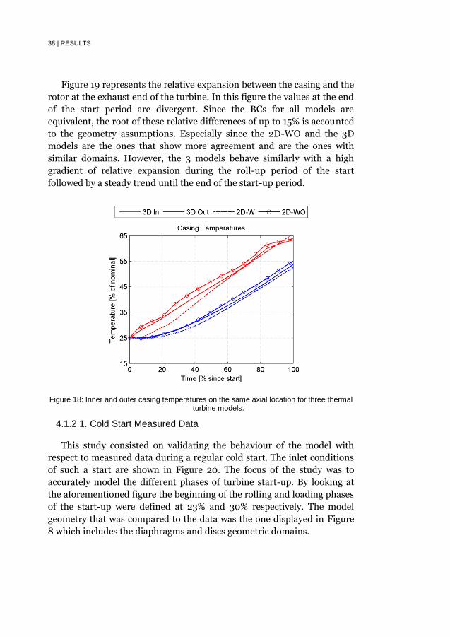
38 | RESULTS

Figure 19 represents the relative expansion between the casing and the

rotor at the exhaust end of the turbine. In this figure the values at the end

of the start period are divergent. Since the BCs for all models are

equivalent, the root of these relative differences of up to 15% is accounted

to the geometry assumptions. Especially since the 2D-WO and the 3D

models are the ones that show more agreement and are the ones with

similar domains. However, the 3 models behave similarly with a high

gradient of relative expansion during the roll-up period of the start

followed by a steady trend until the end of the start-up period.

Figure 18: Inner and outer casing temperatures on the same axial location for three thermal turbine models.

4.1.2.1. Cold Start Measured Data

This study consisted on validating the behaviour of the model with

respect to measured data during a regular cold start. The inlet conditions

of such a start are shown in Figure 20. The focus of the study was to

accurately model the different phases of turbine start-up. By looking at

the aforementioned figure the beginning of the rolling and loading phases

of the start-up were defined at 23% and 30% respectively. The model

geometry that was compared to the data was the one displayed in Figure

8 which includes the diaphragms and discs geometric domains.

RESULTS | 39

Figure 19: Differential expansion at turbine exhaust for three thermal turbine models.

Figure 20: Measured data of cold start inlet conditions.

Figure 21 and Figure 22 show the comparison results for casing

temperatures at the turbine inlet and differential expansion at the

exhaust end of the machine, respectively. Overall, good agreement

between the calculated and measured values was obtained, especially

from the rolling up phase onwards. In the pre-warming phase, it can be

40 | RESULTS

seen in Figure 21 that the trend of the curves is not equal. This is

accounted to two reasons. One of the reasons is related to a slight speed

increase occurring at 20%-since-start which is not captured by the

thermal model. The other reason is the difficulty to model and capture the

impact of the low flow conditions of the gland steam to the casing. This

has also been a difficulty encountered in other studies [9]. However, this

divergence at the beginning of the start is rapidly made up as soon as the

temperature gradients from the incoming live steam take over during the

rolling phase.

Figure 21: Mid casing temperature on the same axial location of turbine thermal model and measured data.

It is important to observe the differential expansion behavior with

more detail in this section. As seen in Figure 22 for both the measured

data and the calculated values, during the pre-warming stage the

differential expansion is relatively constant and driven by the initial

temperature differences in the rotor and casing components from the

cool-down period preceding the start. As expected, the rotor remains

warmer than the casing during cool-down and therefore the differential

expansion for this stage is positive.

The highest differential expansion is reached at the front of the start

when the rolling-up phase begins. At this stage the rotor expands faster

than the casing. This occurs due to the fact that the HTCs in the rotor

discs are much higher than those in the casing diaphragms since

RESULTS | 41

rotational speed enhances heat transfer rates. However, once the speed

becomes steady and the loading begins, the response of the casing begins

to equalize and eventually overcomes the rotor. This is observed in the

negative values of differential expansion. Towards the end of the start, as

steady state conditions are reached, the differential expansion also

becomes steady with the casing more expanded than the rotor.

Figure 22: Differential expansion at turbine exhaust of turbine thermal model and measured data.

Sensitivity Studies on Boundary Conditions

The BCs that were found to have the largest influence towards

capturing the differential expansion in §4.1.2.1 were those related to the

bearings and the inter-casing cavity. Their effects were most influential in

the loading phase of the start in which the casing begins to grow faster

than the rotor. A sensitivity study was carried out varying the

assumptions for these BCs. The bearing oil BC was varied from being

negligible to assuming that the oil is not heated by rotational friction. The

cavity BC was varied from assuming saturation steam temperatures to

assuming the same temperature as in the live steam of the corresponding

turbine stage. The HTC for the cavity was re-calculated for each assumed

temperature.

Figure 23 shows the upper and lower bounds obtained for the

differential expansion due to the variations of the heat transfer conditions

42 | RESULTS

on these surfaces. For both cases a wide range of impact was obtained,

therefore efforts were made in understanding the effects that these BCs

induce to the overall thermal expansion of the casing and rotor

components. An objective of such understanding was to ensure that the

selected assumptions for the final calculated values were in accordance to

the on-going physical principles and not assumed only to match the

measured data.

Figure 23:: Sensitivity of differential expansion to bearing oil and cavity steam heat transfer conditions.

In Figure 23 it can be observed that the effect of the bearing oil BC is

more relevant in the period after rolling. The shaft is cooled with

lubrication oil around the bearings, which implies that this is the only

heat transfer occurrence in the shaft that yields a negative axial

expansion. This results in a delay of the relative growth of the rotor with

respect to the casing which eventually allows the casing to become equally

expanded. Therefore, taking into account bearing oil temperature is an

assumption that should not be neglected when considering thermal

expansion modeling. Since the mass flow of lubricating oil was not in the

scope of the model, minimum and maximum values for the oil

temperature were defined and associated with the minimum and

maximum speed of the start. Such values were selected in accordance

with safety limits of common industrial practices of keeping the bearing

oil temperature between 45oC and 85oC [8].

RESULTS | 43

The assumption of the temperature and HTC of the steam that leaks

into the inter-casing cavity also plays an important part in the expansion

rate of the casing during the loading stage Similar to the bearing oil,

Figure 23 shows how the effect of these assumptions are more relevant

after roll-up. However, its main effect is related to the fact that higher

heat transfer conditions in this area increase the rate of expansion in the

casing, therefore allowing it to expand up to the same level as the rotor.

There is a certain level of uncertainty when it comes to defining the heat

transfer conditions in this region. Presently, all existing data is not yet

sufficient for accurate generalized correlations. One of the main

challenges is to set the dependency between the steam temperatures in

the mainstream and within the chamber [3].

4.2. Model Implementation

With the interest of reducing the drawbacks related to transient

operation and increasing the operational flexibility of steam turbines, the

validated model was implemented in parametric studies. The purpose of

such studies was to look into improving the operation of steam turbines

during transients.

The prediction of the correct thermal behavior of the turbine with the

use of the steam turbine thermal model has allowed for parametric

studies towards achieving shorter start-up times to be performed in the

past [10] [11]. In those studies, the main investigated property was the

temperature distribution throughout the turbine metal, more specifically,

the temperature at the casing near the turbine inlet. The relevance of the

casing temperature is related to the fact that this is a measurable property

in fielded turbines. Furthermore, this temperature is commonly used as

the reference temperature for determining the type of start-up curve to

apply.

The implementation of the model in this work continues in a similar

direction. Two main groups of para metric studies were carried out, both

of which are related to implementing temperature maintaining

modifications in the turbine. One of them investigated the potential

startup time reduction while the other focused on reductions of the peak

thermal expansion during start.

44 | RESULTS

4.2.1. Start-up Time Reduction

4.2.1.1. Temperature Maintaining Modifications

A potential area for increased turbine start-up flexibility involves

maintaining higher internal temperatures during offline periods.

Therefore, in order to increase the flexibility of the turbines while

preserving lifing requirements, three operational modifications for

maintaining turbine temperatures during offline periods were proposed

and investigated.

In previous works developed within KTH, temperature maintaining

modifications for solar steam turbine start-up time reduction have been

studied [10][11]. The operational modifications that were analyzed

involved increasing the turbine insulation thickness, using heat blankets

in the casing and increasing the temperature of the injected gland steam.

Results indicated a great potential for maintaining the turbine

temperature when combining the effects of the heat blankets and the

gland steam temperature increase. The combined modifications showed

an increase in power output of up to 9.5% on the day following a long-

cool down [10]. In addition, an annual performance improvement of 3.1%

for the entire plant was predicted when applying these modifications [11].

In addition to the previously studied measures, there were other

temperature maintaining modifications worth exploring. The

modifications studied included:

increasing the gland steam pressure injected to the end-seals,

Increasing the back pressure,

Increasing the barring speed.

These three measures were applied during turbine stand-still in order

to obtain more favorable temperature profiles in the turbine at the time of

start-up. The first measure consists of increasing the mass flow of gland

steam injected into the turbine by increasing its pressure. The second and

third are related to warming the turbine through the use of friction and

ventilation work. This is achieved either by increased back-pressure

and/or by higher turning gear speed. Although ventilation and friction

are normally considered to be losses in a turbine stage [16], their

implementation for heating purposes and start-up optimization exist has

been considered by Yuichi et al.[41] and in the VGB Guidelines [6].

RESULTS | 45

The modifications were implemented in the dynamic thermal turbine

model after the proposed operational improvements were included as

variable inputs. The effects of the modifications were invstigated through

parametric studies which applied the operational modifications to the

modeled turbine in individual and combined approaches. The potential

improvements were quantified by comparing the temperature obtained

with the combined modifications to regular turbine cool-down

temperatures. The comparison showed significant improvements on the

start-up times of the turbine.

When modeling the operational modifications for the turbine,

limitations from the remainder of the power plant were not taken into

account. The studies performed on the model are thus parametric, and

the necessary time for the operational modification to be effective from

the power plant to the turbine is not taken into account. This is most

relevant to the measures of increasing back pressure and barring speed,

due to the fact that pressurizing a turbine or increasing its speed is

something that requires a certain time to implement at the power plant

level. However, the parametric studies performed in this work serve as a

first analysis of the existing potential for start-up improvement.

Increase of Gland Steam Pressure

In previous work performed in KTH, increasing the gland steam

temperature was studied as a measure for keeping the turbine warm

during barring [10]. This modification showed a strong positive influence

on maintaining the rotor temperatures as well as a lesser influence on the

casing temperatures. However, issues with respect to inducing thermal

stresses on the low pressure side of the rotor limited the range of

application of the measure. In this work, the temperature was kept

constant and the gland steam pressure was increased instead in order to

increase the mass flow. This measure was applied on both the high and

low pressure end seals of both turbine units.

As dictated by the nature of Fanno flow [42], by increasing the inlet

pressure of the gland steam the mass flow through the seal also increases.

Manipulating equation (3) with the ideal gas law equation reveals the

gland steam mass flow to be directly proportional to the inlet pressure

and inversely proportional to the square root of the temperature.

Therefore, the implementation of this measure represents a higher heat

46 | RESULTS

transfer coefficient at the level of the seal and it also provides a greater

source of heat inside the turbine from the increased inwards leakage.

Increase of Back Pressure

Given that friction and ventilation work result in lower turbine

efficiency during operation, these two phenomena are generally viewed as

a problem rather than a solution. Particularly, uncontrolled temperature

increases in idling back pressure turbines is a well-known disturbance

that results from ventilation [43]. However, from the perspective of

maintaining the turbine temperature during cool-down, the effects of

friction and ventilation can be viewed as a source of heat within the

turbine. Moreover, the latter mechanism also feeds work to the trapped

steam by addition of swirl to the flow. As shown in Equations (5) and (7),

the work is proportional to the density of the trapped steam. Increasing

the back pressure of the turbine units will therefore have a direct effect on

this density and will increase the heat produced by friction and

ventilation.

In regular power plant operation, turbine barring is generally

performed at nominal condenser pressure. An increase of back pressure

can be achieved by simply increasing the condenser pressure during

barring. In order to maintain vacuum conditions within the turbines,

which prevent corrosion issues, the back pressure increase is limited to

values below atmospheric pressure. For the case of the HPT, higher back

pressures can be achieved by adding a control valve at the outlet which

can be closed during barring [41]. This can be done in any double by-pass

turbine configuration in the pipe line that connects the outlet of the HPT

directly with the condenser. When applying the proposed operational

measure, it is necessary to ensure that temperatures in the LSB do not

reach unacceptable levels [44].

Increase of Rotational Speed

Turbine barring at increased speeds is simply another way of taking

advantage of the effects explained in the previous section. Equations (5)

and (7) depend on the cube of the rotational speed. Therefore, by

increasing the barring speed, the heat source from friction and ventilation

will be higher. Once again, the range of application this modification is

limited by the temperatures reached in the LSB.

RESULTS | 47

4.2.1.2. Individual Temperature Impact

When simulating the turbine with the proposed modifications, two

main scenarios were considered and consist of an initial phase of 8 hours

of nominal operation followed by either a short or long cool-down period

of 10 and 24 hours respectively. These scenarios are representative of real

turbine operation in CSPPs. Concerning start-up, it is the final

temperature within the turbine before start-up that determines the

selection of the start-up cover, and these temperatures have been

evaluated at both the casing and rotor.

As a first study, the impact of each modification on the turbine

temperatures was calculated separately. The relevant parameter of each

modification was varied while the others were kept at constant nominal

values. For each case, the temperature improvements were calculated

from the difference between the final temperatures obtained when

applying the modification and the one obtained from the base case. The

base case was defined as nominal cool-down of a standard turbine

installation, without any modifications applied, neither those proposed in

this paper nor those studied in previous works [10].

The temperature improvements were measured in the casing and in

the rotor. This was done at an axial location near the inlet due to the fact

that these are critical thick-walled areas which are exposed to high

temperature gradients. In addition, current start-up curves are based on

these temperature measurements. Figure 24 shows the temperature

improvements obtained for each modification on the HPT and LPT

during short and long cool-down periods.

One of the first things to be noticed is how the temperature

improvements are generally higher for the long cool-down periods than

for the short ones. This makes sense given that after a long cool-down the

overall temperatures on the turbine are lower, meaning that the

modifications have a larger potential to increase the turbine temperature

due to the larger temperature difference.

From the impact of increasing the gland steam pressure it can be seen

that the modification has a low impact on the casing of the turbines but a

greater influence on the rotor. This is to be expected given that the rotor

measurement point is in direct contact with the gland steam flow, while

the casing measurement point is subject to conductive diffusion and heat

losses through the insulation and the atmosphere. The overall influence

of this measure on the HPT is low.

48 | RESULTS

Figure 24 Temperature improvements in the rotor and casing after individually applying each of the three improvements to the HPT and LPT.

These temperature improvements are comparable to those obtained

when increasing the gland steam temperature [10] with respect to the

higher influence in the rotor than in the casing. However, the magnitude

of the improvements by increase of gland temperature is one order larger

than that by increase of pressure. Furthermore, it can also be seen in

Figure 24 that after a certain amount of pressure increase the

improvement becomes asymptotic. This non-linear relation between the

pressure increase and metal temperature improvements agrees with the

nature of the modification and is related to the increase of the gland

steam mass flow, as shown in Equation (3).

Results from increasing the back pressure show a high impact both in

the rotor and the casing. Likewise, by increasing the rotational speed

similar effects are obtained in these two turbine components. The reason

for this is that the heat transfer mechanisms being affected are ventilation

and friction work, which act upon the turbine discs and blades and these

are connected both to the stationary and rotating parts of the turbine.

Furthermore it can be seen that by increasing the back pressure,

temperatures improve linearly, while by increasing the speed,

RESULTS | 49

temperatures improve cubically. This is in line with the dependencies

from Equations (5) and (7).

When looking at back pressure and barring speed increase, apart from

the shape of the curves, similar behavior with respect to the temperature

impact of the modification on each turbine component can be seen in

Figure 24. This is related to the fact that the sum of ventilation and

friction work is equivalent in each case. In both cases, ventilation work is

dominant over friction work. In addition, the dependency of the friction

correction factor to the rotational speed through the rotational Reynolds

number, Equation (6), also affects the fact that the resultant work is

similar in both modifications.

For the LPT, in both cases it is seen that the casing impact is larger

than the rotor. While for the HPT the rotor and the casing are affected

similarly. This is due to the fact that each turbine is sized in differently;

the larger dimensions of the LPT result in larger temperature differences

between the components.

Although significant temperature improvements can be achieved by

the measures when applied individually, it is proposed to combine the

three in order to quantify the complete range of possible impact on the

turbine temperatures. After the individual implementation of the

proposed modifications, it is seen that increase of back pressure and

barring speed are the ones that have the larger potential for temperature

improvements. Therefore, the combination of these two modifications is

considered in upcoming sections.

4.2.1.3. Turbine Cool-Down Behavior

Before performing the combined study of the operational

modifications, a discretization of the range of application should be

performed. As was noted before in §4.2.1.1 , the application of increased

back pressure and barring speed are constrained by undesired heating in

the LSB. In the previous section, their implementation was done without

any limitations in order to obtain the prospective temperature

improvements for the turbines that the measures could provide.

Furthermore, it also served to observe the different levels of impact in the

casing and in the rotor. However, the allowed range of application must

be analyzed before combining the measures and drawing any results

related to start-up time reduction. It is desired to take advantage of these

modifications without incurring in any lifing risk for the turbine.

50 | RESULTS

As mentioned in §4.2.1.2, the results shown in Figure 24 were

calculated at an axial position near the turbine inlet as this is how is done

in current industrial applications for determining start-up curves.

However, the heat sources from ventilation and friction tend to heat the

turbine outlet section more than the inlet due to their dependency on the

disc diameter and blade length. In order to evaluate the overall

temperature profiles from turbine inlet to outlet, several points

distributed along the axial direction, mainly in the blade passage area,

were selected. Temperature profiles were then calculated in the rotor and

in the casing of the turbines for three main scenarios:

Nominal operating state: just before a cool-down (CD) period.

Nominal cooled down state: after a short or long cool-down period.

Modified cooled down state: after a short or long cool-down period

with the combined measures implemented.

Figure 25 shows the different cool-down behaviors in the turbine

components.

Figure 25 Temperature profiles along the axial direction if the casing and rotor of the HPT and LPT for nominal temperature state and cool-down states

Each modified cool-down curve shows a different combination of the

modifications, namely increased back-pressure and barring speed.

Similar to the individual implementation figures, in these figures the

metal temperatures increase along with the magnitude of the modified

parameters. The nominal cool-down behaviors on each figure show the

temperature state after the long cool-down to be at a lower level than the

short cool-down. This occurs especially in the inlet section where the

temperature differences to the atmosphere (for the casing) and/or the

RESULTS | 51

bearings (for the rotor) are much larger and so are the heat losses. In

addition, some of these figures show the cooled-down state at the outlet

to be warmer than the nominal state. This is due to the fact that during

nominal operation the temperatures at the outlet are ruled by the steam

expansion, while for cool-down the temperatures are redistributed axially

and the external gland steam temperature slightly warms the exhaust

section.

In general, Figure 25 clearly portrays how the heat generated from

ventilation and friction greatly affects the outlet side of the turbines, even

reaching critical values in some cases. Heating this section of the turbine

brings no value to current turbine start-up technologies and it would

generate undesired thermal stress at the moment of operation. Besides,

the aim of the proposed modifications is to maintain the turbine

temperature with respect to the last operating temperature state and not

increasing it beyond this point. Therefore, the initial range of application

of the individual modifications was discretized to avoid excessive

overheating in the exhaust.

The main limiting criterion for the application of the measures was

based on thermal loading constraints. This is related to the casing and

rotor permissible transients, which allow relatively large additional

thermal loading at component temperatures below 400○ C [6]. In

addition, power plant feasibility constraints were also considered for

discretizing the range of application. These are related to the achieved

exhaust steam temperature and the initial temperature difference of the

condensing system of the power plant in the case of operation [44]. The

limiting temperature state resulting from the combination of the

modification and fulfilling the criteria is shown on Figure 25 as the solid

modified CD curve. However, additional turbine design restrictions would

have to be considered beyond this limited state in order to include

specific local stage effects and their limitations.

4.2.1.4. Combined Temperature Impact

Once safe limits at the temperature level were established on the range

of application of the combined measures, their impact with respect to

temperature improvements and start-up time reductions were studied.

The combined measures scheme simply involved taking the allowed range

of application of each individual measure and calculating the entire map

of possible combinations. Although the back pressure and the barring

52 | RESULTS

speed are the main varying parameters due to their potential, a fixed

value of increased gland steam pressure was also selected as part of these

combinations. This value was selected within the range in which the

temperature improvements from increased gland steam were asymptotic

(Figure 24).

Figure 26 and Figure 27 show the impact of the combined measures

on the rotor and casing temperatures. When compared with the

individual studies at the relevant points, a higher impact can be observed

even with the limited range of application. The HPT shows a higher

degree of temperature improvements than the LPT. This is due to the fact

that the range of application of the measures is much wider for the

former. The range for the LPT is more limited as a consequence of its

longer blades and higher ventilation temperatures in the outlet.

Furthermore, when comparing the casing and the rotor outcomes for

each turbine a similar behavior as discussed in §4.2.1.2 is observed. The

components of the HPT are similarly affected by the modifications, while

the components of the LPT show significant temperature differences from

casing to rotor.

4.2.1.5. Start-up Improvements

The start-up time improvements achieved for the allowed range of

application of the combined measures of back pressure and barring speed

increase are also shown in Figure 26 and Figure 27. This was done by

showing the relevant metal temperature increase that would imply a

change of start-up curve and thus, start time improvement. The time

improvements are shown on the figures as a percentage of the start-up

time without applying the modifications.

With its wider range of modification application, the HPT showed the

most potential for start-up time reduction with improvements of up to

70% from the initial start-up time. Conversely, the start-up time

reductions for the LPT only reached 9.5%. This is not only related to the

range of application but also to the increased thermal inertia of the

machines due to size and dimensions.

Also, another notable issue is how for each turbine the short cool-

down case showed improvements only at the limit of application of the

measures. This is related to what was mentioned in §4.2.1.2 about the

lower potential that the modifications have to impact the turbine during

the short-cool down due to the smaller temperature differences and this

RESULTS | 53

can be observed by comparing the short and long cool-down scenarios in

Figure 25.

Figure 26 Temperature improvements in the rotor and the casing of the HPT after applying the combined modifications.

For a given combination of the measures, it was seen that the achieved

temperature improvements are not equal for the casing and the rotor of

the turbines. This is especially true for the case of the LPT unit. Therefore,

the potential for start-up improvements on each component do not occur

simultaneously. Under current industrial practice the start-up curves are

determined based on casing measurements only, given that the rotor is

inaccessible for temperature measurements. The rotor temperature states

are estimated based on the measurements of the casing. Since the rotor is

at a more elevated temperature state, in Figure 26 and Figure 27 is shown

how the start-up time improvements occur at an earlier stage of the

54 | RESULTS

application of the combined measures. This reflects on the importance of

accurate predictions of rotor temperatures for start-up time

determination, if the temperature states were to be reversed and only the

casing temperatures are considered, then serious damage would occur in

the rotor. In addition, it also highlights the importance of implementing

modifications that improve both the rotor and casing temperature states,

due to the fact that the less favored component is the one that determines

the start-up.

Figure 27 Temperature improvements in the rotor and the casing of the LPT after applying the combined modifications.

4.2.2. Differential Expansion Reduction

The sensitivity studies performed in this section were oriented

towards reducing the maximum differential expansion that occurs during

the rolling up phase of the start, as observed in Figure 22 . A straight-

RESULTS | 55

forward way of reducing this peak value has to do with keeping the casing

warmer during cool-down and therefore increasing its initial temperature

at the time of start. Building on the results from the previous section, as

well as from previous works [10], warming of the casing can also reduce

thermal stress and through that enhance the start-up ramps. For this

parametric study, the initial temperature of the casing was simply

increased in order to observe the effects on the maximum differential

expansion.

There were two approaches considered when increasing the casing

temperature. One approach consisted in increasing the initial

temperature of the whole casing. The other approach consisted of a more

detail analysis to localize the critical sections on the casing which require

being warmer at the time of start. The localization of critical sections for

the second approach was done by observing the individual thermal

expansion in various axial locations of the turbine in the timeframe in

which the peak of differential expansion occurs.

The axial profile of differential expansion at the different locations is

observed in Figure 28. As it can be appreciated in the figure, the locations

are not evenly spread out in the axial direction. This is due to the fact that

the selection of the locations was based upon occurrences of significant

transitions in BCs or relevant geometric changes. It is important to

highlight that location “ ” is at the thrust bearing collar and is therefore

the reference location for zero axial expansion. Furthermore, locations

and mark the beginning and end of the blade passage, respectively.

Location represents the closest point in the model to where the

differential expansion measurements are taken from the fielded turbine.

For the selected time instants, the rotor is more expanded than the

casing in all locations except point . This is related to the fact that

evaluation point is located at the end of the thrust bearing and therefore

the effects of the cooling oil discussed in end of §4.1.2.1 apply. The casing

locations that were considered as critical were those in which the

differential expansion was highest at the instant of the peak, namely

location .

56 | RESULTS

Figure 28 Measurement locations of axial displacement in turbine geometry (left) Individual differential expansion at measurement locations for time instants in the vicinity of

the peak value of differential expansion during rolling-up.

Once having identified the critical location in the casing. The

parametric study was carried out for the two approaches. This was done

by calculating the maximum differential expansion for different casing

temperature increases. Figure 29 shows the comparison of the differential

expansion reduction between the global and local approaches. In general,

both approaches yield reductions for the peak of differential expansion.

The global approach has a considerably higher rate of reduction than

the local approach. This is expected as the whole volume of the shell is

being heated as compared to only one localized section. In this regard, the

localized approach can be considered to be more feasible and effective;

even more so when considering its industrial implementation, since

keeping only a certain part of the casing warm implies less parasitic

consumption. However, a drawback of the localized approach would be

the increased risk to thermally distort the casing, which could also lead to

rubbing.

One important aspect to be highlighted from Figure 29 is that there

are limits to how much the casing temperature can be increased. Besides

obvious restraints related to allowable material and operating limits, the

temperature increase of the casing is constrained by the fact that this

induces negative differential expansions to the case at hand. This can be

seen in the curve for the global approach in Figure 29, in which there are

no further reductions in the maximum peak of expansion after a certain

casing temperature increase. At this point, the maximum expansion is no

longer occurring in the expected location but is instead being shifted to

the negative side of expansion.

RESULTS | 57

Figure 29: Reduction of the maximum differential expansion due to global and localized casing initial temperature increase.

58 | CONCLUSIONS

5. Conclusions

Current power plant operation requires more dynamic steam turbine

components. This raises the interest of achieving faster turbine start-ups

in order to adapt quickly to the fluctuations in energy supply to the

market. Turbine start-ups are governed by curves which limit the time it

takes for the turbine to reach nominal load and speed. The main objective

of the start-up curves is to protect the turbine component from

detrimental phenomena which occur as a consequence of transient

operation. Radial thermal stresses in thick walled components and axial

rubbing between stationary and rotating parts due to relative axial

expansion are among these negative phenomena.

In this work, a turbine thermal model was validated and implemented

in parametric studies concerning improvements of the thermal behavior

during start-up conditions. These sensitivity studies were performed in

order to understand existing constraints of turbine start. In order to

perform such studies a turbine thermal model was developed based upon

previous work from KTH [10]. The previous model was modified and

refined in terms of geometric adaptability and heat transfer assumptions.

This was done in order to deliver a fast calculating tool of sufficient level

of detail to accurately capture transient behavior of all turbine

components. Furthermore, it was also desirable for the modeling scheme

to be easily adaptable to other turbine models for future work. The

developed modeling tool also differed from other works as it did not

comprise calibration with instrumented turbines [7] [8] or

computationally cumbersome CFD calculations [9].

Validation studies were carried out in order to verify the impact of the

geometric simplifications and heat transfer assumptions made on the

model. The comparisons of the model were done against other numerical

models of higher geometric detail and against measured operational data.

The geometric comparisons showed that the 2D axisymmetric modular

model was able to capture the same dynamics of the temperature

fluctuations as the continuous geometric approach and the 3D FE model.

In the comparisons with the latter, when assuming the same geometric

CONCLUSIONS | 59

domains for the 2D model (2D-WO) the effect between the models were

the same. When considering the diaphragms and rotor discs domains it

was found that geometric assumptions affect the thermal inertia of the

model while still maintaining the behavior with respect to temperatures

and differential expansion. The modular geometric approach is therefore

considered to be adaptable to different turbine geometries while still

accurate for surface temperature predictions. The comparisons against

measured operational data yielded overall good agreement for the two

studied turbines. During this comparison process, sensitive boundary

conditions and their influence towards capturing the differential

expansion behaviour of the turbine were identified at the bearings and

the inter-casing cavity.

The implementation of the model in parametric studies was focused

on exploring the impact of temperature maintaining modifications in the

modeled turbines. This impact was studied in terms of start-up time and

differential expansion. As a general rule for start-ups, the warmer the

turbine is before the start, the faster the start-up can be. Therefore, on

this work three temperature-maintaining operational modifications were

considered: increase of gland steam pressure, increase of back pressure

and increase of rotational speed. When considering the combined

measures, improvements on start-up times of starting from 9.5% and

reaching up to 70% were obtained.

In parallel, the casing initial temperature was varied in order to

explore its effect on the peak differential expansion during start. In the

study the casing temperature was increased in two ways: globally and

locally. Reductions of 37% and 20% were obtained for the global and local

casing increases respectively. However, limitations in the range of

application of the measure existed. These limitations were related to

inducing negative differential expansions and to 3D effects of casing

distortion which are not studied by the model.

In general, accurately predicting the thermal behavior of the turbine

directly affects studies on start-up optimization, thermal stresses and

LCF. The modeling approach developed and validated in this work serves

as a basis to perform temperature prediction studies on different steam

turbines subject to varying operating conditions. The studies performed

in this thesis represent a step towards achieving faster and reliable

turbine start-ups. Maintaining the temperature of the steam turbines

during offline periods seems to be a viable possibility for achieving

60 | CONCLUSIONS

flexibility during start-up. Furthermore, understanding the differential

expansion behavior of a turbine serves as a base towards establishing

faster start-up strategies and involving clearance controls during


5.1. Future Work

This licentiate thesis has been performed as part of on-going research

at KTH. Therefore, this thesis does not represent the conclusion of the

work. Research on the topic of steam turbine optimization for flexibility

at start-up will continue as there remain a number of aspects to

investigate in depth.

One of the main focuses for future work will be related to furthering

the validation of the model. Although satisfactory results were achieved in

this work, there were mostly focused on HPT geometries. Future work

will involve considering different type and sizes of turbines. This will

enrich the developed modeling tool as every turbine model involves its

own set of particularities in terms of heat transfer, geometry and 3D

effects. With respect to the modeling tool, future work will involve

refining its capabilities in order to enable the location of the highest stress

points, allowing use of the model for establishing new start-up curves.

It should be noted that the results obtained in this paper with respect

to the operational modifications are relevant to only two specific cool-

down cases. In addition, the influence of the entire power plant on the

implementation of these modifications was not considered in the thesis.

For future work, a complete annual cool-down distribution along with the

implementation of these measures at power plant level will be studied,

along with related cost analysis.

Additionally, future work will involve studying additional

modifications to the steam turbines in order to define and improve the

thermal limiting criteria. These measures will be related to control, design

material and operation strategies. Finally, based on these modifications

and evaluations against allowable temperature differences the design of

generalized strategies for faster steam turbine and power plant start-up

will be proposed.

All these issues will be examined in future PhD work.

REFERENCES | 61

References

[1] World Energy Scenarios: Composing Energy Futures to 2050. Rep. no. 4184478.

London: World Energy Council, 2013.

[2] Birnbaum J, Feldhoff JF, Fichtner M, et al. Steam temperature stability in a direct steam

generation solar power plant. Solar Energy. 2011;85(4):660–668.

[3] Leizerovich A. Steam turbines for modern fossil-fuel power plants. 10th ed.; 2008.

[4] Kosman G, Rusin A. The influence of the start-ups and cyclic loads of steam turbines

conducted according to European standards on the component’s life. Energy.

2001;26(12):1083–1099.

[5] Jöcker M, Wikström R, Nyqvist J. Steam Turbine Optimization for Operation in Thermal

Solar Power Plants. In: PowerGen Europe Conference. Germany; 2012:1–16.

[6] VGB PowerTech. Thermal Behavior of Steam Turbines. VGB-R 105 e .VGB PowerTech

.e.V.; 2nd ed; 1990.

[7] Marinescu G, Ehrsam A. Experimental Investigation Into Thermal Behavior of Steam

Turbine Components: Part 2—Natural Cooling of Steam Turbines and the Impact on

LCF Life. Proceedings of ASME Turbo Expo 2012, Coppenhagen, Denmark.

[8] Marinescu G, Ehrsam A, Sell M, Brunner P. Experimental Investigation in Thermal

Behavior of Steam Turbine Components: Part 3—Startup and the impact of LCF life.

Proceedings of ASME Turbo Expo 2013, San Antonio, Texas.

[9] Brilliant H., Tolpadi H. Analytical Approach to Steam Turbine Heat Transfer in a

Combined Cycle Power Plant. Proceedings of ASME Turbo Expo 2004, Vienna, 2004.

[10] Spelling J, Jöcker M, Martin A. Thermal Modeling of a Solar Steam Turbine with a

Focus on Start-Up Time Reduction. Engineering for Gas Turbines and Power.

2012;134(1)

[11] Spelling J, Jöcker M, Martin A. Annual performance improvement for solar steam

turbines through the use of temperature-maintaining modifications. Solar Energy.

2012;86(1):496–504.

[12] Dixon, S.L., 1998, Fluid Mechanics and Thermodynamics of Turbomachinery, Fourth

edition, Butterworth-Heinemann, Woburn, MA, USA, 1998, ISBN 0-7506-7059-2

[13] Kiameh P. Power Generation Handbook. New York: McGraw-Hill; 2002

[14] GlobalData. Steam turbines in Thermal Power, 2013 Update – Global Market Size,

Average Pricing, Equipment Market Share to 2020. Report number: GDPE1064MAR.

December 2013.

[15] Technology Characterization: Steam Turbines. Arlington: Energy and Environmental

Analysis, 2008.

[16] Leyzerovich A. Large power steam turbines: Design and Operation, Volume I. Penn

Well Books.7th ed.;1997.

[17] Cooke D. Modeling of Off-Design Multistage Turbine Pressures by Stodola’s Ellipse

1983:205–34.

[18] Wittig S., Jacobsen K., Schelling U., Kim S. Heat Transfer in Stepped Labyrinth Seals.

Engineering for Gas Turbines and Power. 1988; 110(1): 63-69.

62 | REFERENCES

[19] Kostyuk A, Frolov V. Steam and gas turbines. 1st ed. Moscow: Mir Publishers; 1988.

[20] Traupel W.,Thermische Turbomaschinen, 3. Auflage, Springer Verlag 1982

[21] Twidell J. and Weir T., Renewable Energy Resources, London: Taylor & Francis, 2006.

[22] World Energy Trilemma: Time to get Real – the case for sustainable energy investment.

London: World Energy Council, 2013.

[23] Grid Integration of Large-Capacity Renewable Energy Sources and use of Large-

capacity Electrical Energy Storage. Market Strategy Board White Paper. International

Electrotechnical Commission, Switzerland, 2012.

[24] Fubi M., Krull F., Ladwig M. Increase in Flexibility with Latest Technologies.VGB

PowerTech Journal 3/2012.

[25] Panek, P., Cerny V., Kapic M., Prchlik L.. Thermal Stress Monitoring and Control

System for Steam Turbines. Power Gen Europe Conference 2012.

[26] CSP Today, 2013, CSP Markets Report, FC Business Intelligence Ltd., London.

[27] Lindström, J., Fällman S., Lyrander M., Gabrielson, C., Requirements and Solutions for

Steam Turbines in Concentrated Solar Power Plants, Proceedings of the POWERGEN

Renewable Energy Conference, Las Vegas, 2007

[28] Nyqvist, J., Haje, D., Kleinerman, K., The Refinement of Industrial Steam Turbines for

Efficient Application in Solar Thermal Power Plants, Proceedings of the International

SolarPACES Conference, Perpignan, 2010

[29] Kolb G., Ho c., Mancini T., Gary J., Power Tower Technoloy Roadmap and Cost

Reduction Plan. Sandia National Laboratories, Report SAND2011-2419, April 2011.

[30] Birnbaum J., Feldhoff J., Fichtner M., Hirsch, T., Jöcker, M., Pitz-Paal, R. et al., Steam

Temperature Stability in a Direct Steam Generation Solar Power Plant, International

SolarPACES Conference, Berlin, 2009

[31] Stuetzle T., Blair N., Mitchell J. et al., Automatic Control of a 30 MWe SEGS VI

Parabolic Trough Plant, Solar Energy, Volume 76 (2004), pp. 187-193

[32] Emberger H, Schmid E, Gobrecht E. Fast Cycling Capability for New Plants and

Upgrade Opportunities. Siemens Power Generation ( PG ), Germany. Siemens. 2005:1–

13.

[33] Guédez R. et al. Reducing the number of turbine starts in concentrating solar power

plant through the integration of thermal energy storage. Proceedings of ASME TURBO

EXPO, San Antonio, 2013

[34] Aga V., Ehrsam A., Boschek E., Breschi D., Girard R., Thermal Energy Storage and

Turbine Solution for Direct Steam Solar Power Plants with Nominal Power Output During

Storage Discharge. In: Proceedings of the International SolarPACES conference,

Marrakesh, 2012.

[35] Ray A. Dynamic modelling of power plant turbines for controller design. Applied

Mathematical Modelling 1980.

[36] Incropera F, Dewitt D. Fundamentals of Heat and Mass Transfer. New York: Wiley and

Sons; 2007.

[37] Khonsari,M.,Wang,S. On the fluid-solid interaction in reference to

thermoelastohydrodynamic analysis of journal bearings, ASME Journal of Tribology, vol.

113 (1991),pp. 398-404

[38] Kreith, Frank, 1965, Principles of Heat Transfer, Harper & Row Publishers. fourth ed.,

[39] Gülen S.C, Gas Turbine Combined Cycle Fast Start: The Physics behind the concept.

Power Engineering, 2013

[40] Morel N., Gnansounou E., Energetique du Bâtiment, EPFL Laboratoire d’Energie

Solaire, Laussane, 2009.

[41] Yuichi T, Osamu M, Kazunori Y. Reheat Steam-Turbine Plant. .Patent Nr.

JP2007046577-A; Japanese Patent Office, 2007.

REFERENCES | 63

[42] Greitzer E, Tan C, Graf M. Internal Flow: Concepts and Applications. New York.

Cambridge University Press, 2004.

[43] Leyzerovich A. Large power steam turbines: Design and Operation, Volume II. Penn

Well Books.7th ed.;1997.

[44] Bergman D., Gloger M., May G., et al. High Temperature Control in High Backpressure

LP Turbines. Proceedings of the American Power Conference, 1985, Vol 47, pp 219-

229.

steam turbine thermal modeling for improved transient ...765657/fulltext01.pdf · la mejor mamá...

Documents