steady state 1d noe

Steady state 1D NOE

Steady State 1D NOE

•  This experiment (as is any difference method), is extremely demanding for a spectrometer. Obtaining perfect subtraction requires very high instrument and temperature stability. • The saturation pulse generates a certain amount of heat in the sample. To compensate for this heat deposition, the “non-irradiated” spectrum also has a saturation pulse applied with the same power and duration, but placed far from the resonances.

Steady state 1D NOE

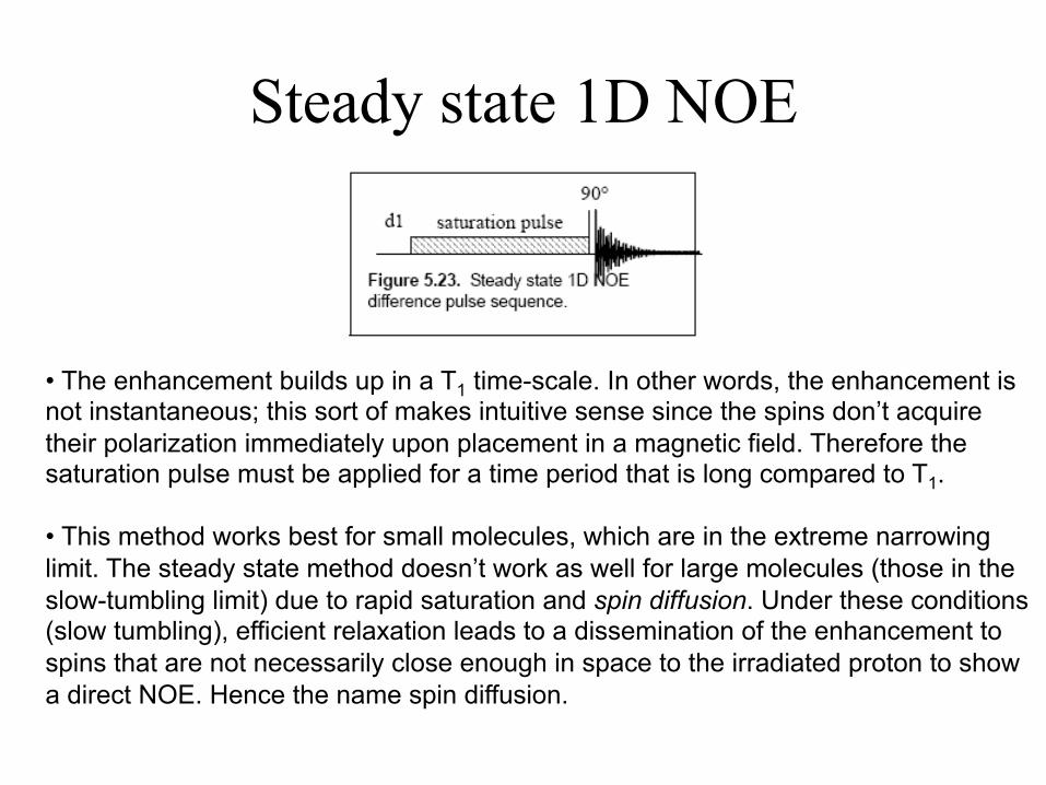
•  The enhancement builds up in a T1 time-scale. In other words, the enhancement is not instantaneous; this sort of makes intuitive sense since the spins don’t acquire their polarization immediately upon placement in a magnetic field. Therefore the saturation pulse must be applied for a time period that is long compared to T1.

•  This method works best for small molecules, which are in the extreme narrowing limit. The steady state method doesn’t work as well for large molecules (those in the slow-tumbling limit) due to rapid saturation and spin diffusion. Under these conditions (slow tumbling), efficient relaxation leads to a dissemination of the enhancement to spins that are not necessarily close enough in space to the irradiated proton to show a direct NOE. Hence the name spin diffusion.

Dependence of the max NOE on ωτc

fI{S}=ηmax=5+ω2τc

2-4ω4τc4

10+23ω2τc2+4ω4τc

4

-1

-0.5

0

0.5

0.01 0.1 1 10 100

0.1 1 10 100

0.5

-0.5

-1.0

ωτc

Small molecules

Large molecules

Extreme narrowing limit

ωI≅ ωS ≅ωγI= γS

5+ω2τc2-4ω4τc

4=0 ⇒ ωτc≅1.12

Steady-state NOE ηI = σIS / ρIS= fI{S}

Steady-state NOE

• What happens is that we have competing relaxation mechanisms for the proton we are saturating (two or more protons in the surroundings). Now the rates of the relaxation with the different protons becomes important (the respective Ws).

•  The equations get really complicated, but if we are still in the extreme narrowing limit, we can simplify things quite a bit. In the end, we can establish a ‘simple’ relationship between the NOE enhancement and the internuclear distances:

•  In order to estimate distances between protons in a molecule we can saturate one nuclei and analyze the relative enhancements of other protons. This is know as steady-state NOE. •  We take two spectra. The first spectrum is taken without an irradiation, and the second with. The two are subtracted, and the difference gives us the enhancement from which we can estimate distances...

rIS-6 - ΣX fX{S} * rIX

-6

fI{S} = ηmax * rIS

-6 + ΣX rIX-6

Steady-state NOE

NOE difference spectroscopy

• If our molecule has three protons, two of them at a fixed distance (a CH2), we have:

Hb

Ha

Hc

Hb Ha Hc

_ = ηab ηac

C

rIS-6 - ΣX fX{S} * rIX

-6

fI{S} = ηmax * rIS

-6 + ΣX rIX-6

Steady-state NOE If we irradiate B, then regardless of how close spin C is to B, we still get roughly a 50% NOE at A (although if C is closer, this is reduced a bit). This analysis assumes there's no dipolar coupling between A and C:

Steady-state NOE But when A is irradiated, you get a positive NOE at B, but a negative NOE at C:

With a four spin system, things get more complicated:

Spin diffusion One of the problems of steady-state NOE is that we are continuously giving power to the system (saturation). This works well for small molecules, because W2 processes (double-quantum) are dominant and we have few protons. •  However, as the size and τc increase, other processes are more important (normal single-quantum spin-spin relaxation and zero-quantum transitions). •  Additionally, there are more protons in the surroundings of a larger molecule, and we have to start considering a process called spin diffusion: •  Basically, the energy transferred from I to S then diffuses to other nuclei in the molecule. We can see an enhancement of a certain proton even if it is really far away from the center we are irradiating, which would give us ambiguous results. •  Therefore, we need to control the amount of time we saturate the system. The longer we irradiate, the more spin diffusion…

I S

Spin diffusion

Hb

Ha

Hc

Hb Ha Hc

_ = ηab ηac

C

Spin diffusion

a) ωτc<<1

Hb

Ha

Hc

Hb Ha Hc

_ = ηab

ηac

C

Spin diffusion

b) ωτc>>1

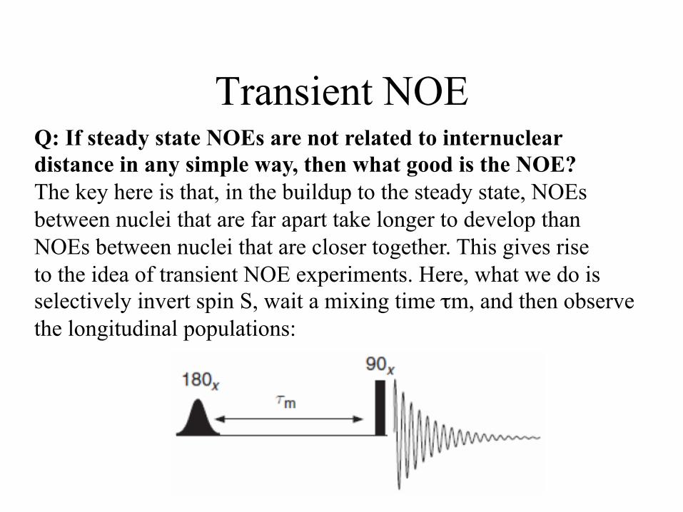
Transient NOE Q: If steady state NOEs are not related to internuclear distance in any simple way, then what good is the NOE? The key here is that, in the buildup to the steady state, NOEs between nuclei that are far apart take longer to develop than NOEs between nuclei that are closer together. This gives rise to the idea of transient NOE experiments. Here, what we do is selectively invert spin S, wait a mixing time τm, and then observe the longitudinal populations:

Transient NOE

IS

αβ

αα

βα

ββ

W1I

W1I W1S

W1S

W2IS

W0IS

+1/2

-1/2

0 0 βα

αα

ββ

W1I

W1I W1S

W1S

αβ

W2IS

W0IS

+1/2 -1/2

0

0

Intensity of I: p(αα)-p(βα)+p(αβ)-p(ββ)=1

Intensity of S: p(αα)-p(αβ)+p(βα)-p(ββ)=-1

0

0

+1/2 -1/2

αα

βα αβ

ββ

0+δ/2

0-δ/2

+1/2 -1/2

αα

βα αβ

ββ

W2IS

Intensity of I: p(αα)-p(βα)+p(αβ)-p(ββ)=1+δ

Transient NOE

IS

0

0

+1/2 -1/2

αα

βα αβ

ββ

0

0

+1/2-δ/2 -1/2+δ/2

αα

βα αβ

ββ

W0IS

Intensity of I: p(αα)-p(βα)+p(αβ)-p(ββ)=1-δ

Transient NOE

IS

Transient NOE

180s 90

tm

selective inversion

tm

ηmax

Transient NOE

dIz/dt = - ρIS(Iz-Iz0) – σIS(Sz – Sz

0)

Iz = Iz0, Sz = –Sz

0

dIz/dt|τm=0 = 2 σIS Sz0

σIS = W2IS - W0IS

ρIS = 2W1S + W2IS + W0IS

σIS: cross-relaxation rate constant ρIS: dipolar longitudinal relaxation

The initial rate approximation

Transient NOE

tm

ηmax

tm

ηmax

Linear build-up

If we also take into account the T1 relaxation:

dIz/dt|τm=0 = 2 σIS Sz0

The angular coefficient of the linear build-up is proportional to σIS

Transient NOE

Ha

Hc

Hb Ha Hc C

ηab ηac

ηab ηac

Hb

Int

τm

Ib

Ic

2Α0σab

2Α0σac

τm

W0IS ∝ γI2 γS

2 rIS-6 J (ωI - ωS)

W2IS ∝ γI2 γS

2 rIS-6 J (ωI + ωS)

σIS = W2IS - W0IS

σIS ∝ rIS-6

σab ∝ rab-6

rac = rab * ( σab / σac ) -1/6 σac ∝ rac

-6

Ha

Hc

C Hb

Transient NOE

Diffusion to X

tm

ηmax

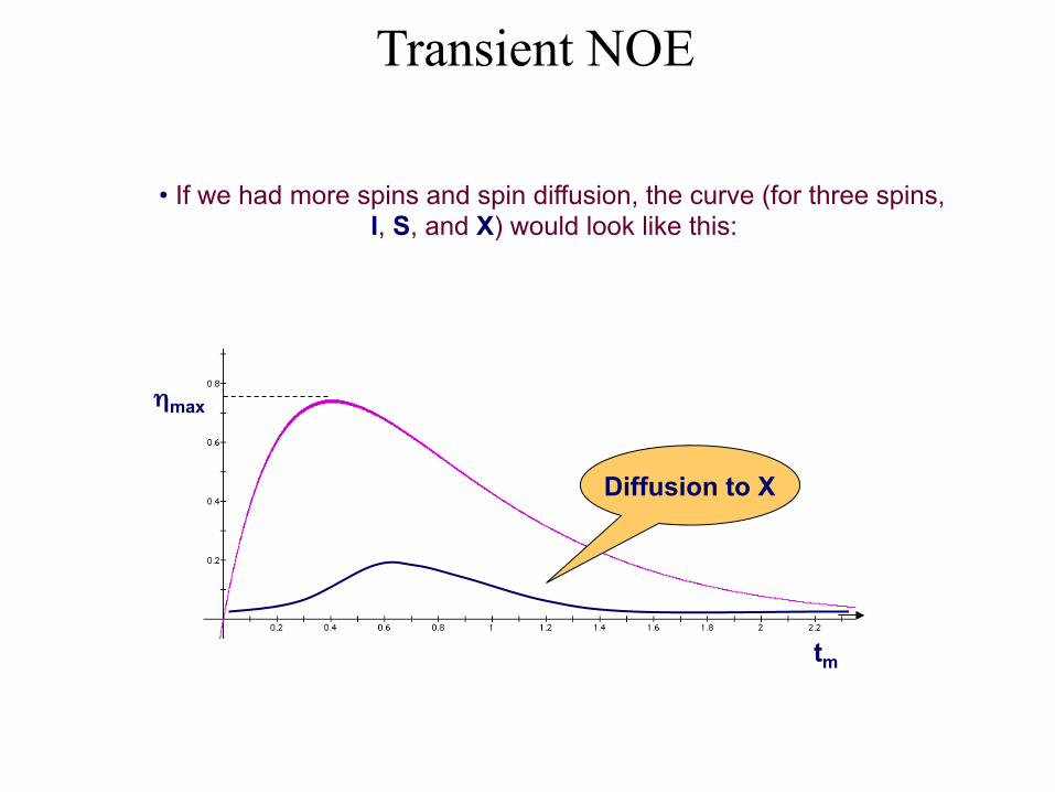
•  If we had more spins and spin diffusion, the curve (for three spins, I, S, and X) would look like this:

Transient NOE

Organic molecules and NOE

NOESY (NOE SpectroscopY)

180s 90

tm

selective inversion

1D Transient NOE

90 90 90

t1 tm

“inversion”

2D NOESY t2

90°x 90°x

1H

t1 t2

-Izcos(ΩIt1)cos(πJISt1) NOESY Experiment

90 90 90

t1 tm

“inversion”

NOESY

COSY

-Izcos(ΩIt1)

t2

αβ

αα

βα

ββ

W1I

W1I W1S

W1S

W2IS

W0IS

+1/2

-1/2

0 0

dI1z/dt = - ρ(I1z-I1z0) – σ(I2z – I2z

0)

σ = W2 - W0

ρ = 2W1 + W2 + W0

“auto”relaxation

“cross”relaxation

αβ

αα

βα

ββ

W1I

W1I W1S

W1S

W2IS

W0IS

+1/2

-1/2

0 0 dI1z/dt = - ρ(I1z-I1z0) – σ(I2z – I2z

0)

σ = W2 - W0

ρ = 2W1 + W2 + W0


0)

ρ= Rauto σ= -Rcross


0)

σ = W2 - W0

ρ = 2W1 + W2 + W0


0)

ρ= Rauto σ= -Rcross

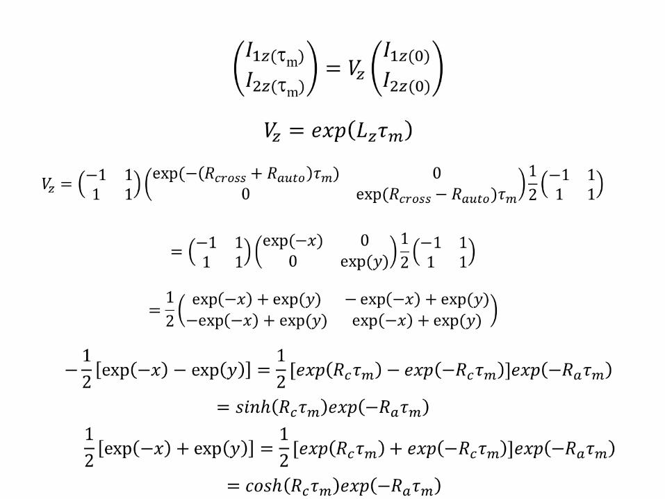
Integration after a t=τm

To calculate the exponential matrix we will diagonalize it

Diagonal matrix

Large Molecules

NOESY Spectra

Small Molecules

NOESY Spectra

90 90 90

t1 tm

“inversion”

NOESY

-Izcos(ΩIt1)

Iycos(ΩIt1)

Iycos(ΩIt1)cos (ΩIt2)

Diagonal peak

σIS

±Szcos(ΩIt1) -Izcos(ΩIt1)

t2

- small molecule + large molecule

∓Sy cos(ΩI t1)

Cross-peak

∓Sy cos(ΩI t1)cos(ΩSt2 )

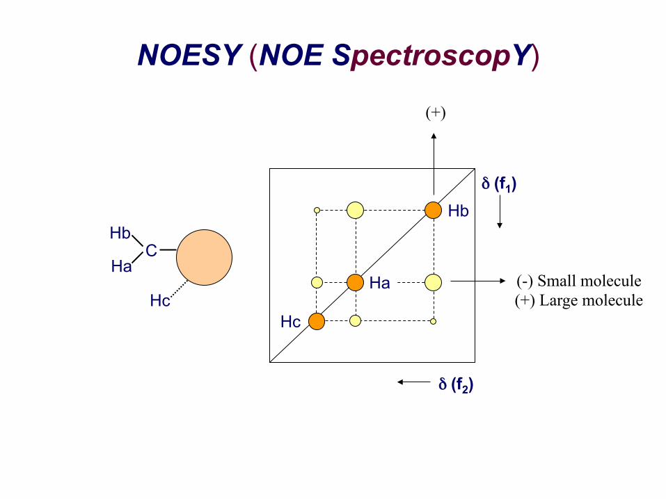
Hb

Ha

Hc

C

Hc

Ha

Hb

δ (f2)

δ (f1)

NOESY (NOE SpectroscopY)

(+)

(-) Small molecule (+) Large molecule

steady state 1d noe

Documents