i

STATUS OF THESIS

Title of thesis MODELING, SIMULATION AND OPTIMIZATION OF INDUSTRIAL HEAT EXCHANGER NETWORK FOR OPTIMAL CLEANING SCHEDULE

I, LOW WAI CHONG

hereby allow my thesis to be placed at the Information Resource Center (IRC) of

Universiti Teknologi PETRONAS (UTP) with the following conditions:

1. The thesis becomes the property of UTP

2. The IRC of UTP may make copies of the thesis for academic purposes only.

3. This thesis is classified as

√ Confidential

Non-confidential

If this thesis is confidential, please state the reason:

The present study is part of a major funded research project which is governed by the

confidentiality agreement with the funding body.

The contents of the thesis will remain confidential for 5 years.

Remarks on disclosure:

Nil Endorsed by ________________________________ __________________________ Signature of Author Signature of Supervisor

Permanent address: Name of Supervisor

A-12-4, Mentari Condo Assoc. Prof. Dr. M. Ramasamy Jln. Tasik Permaisuri 3 Bandar Tun Razak 56000 Kuala Lumpur Date : _____________________ Date : __________________

ii

UNIVERSITI TEKNOLOGI PETRONAS

MODELING, SIMULATION AND OPTIMIZATION OF

INDUSTRIAL HEAT EXCHANGER NETWORK

FOR OPTIMAL CLEANING SCHEDULE

by

LOW WAI CHONG

The undersigned certify that they have read, and recommend to the Postgraduate

Studies Programme for acceptance of this thesis for the fulfilment of the requirements

for the degree stated.

Signature: Main Supervisor:

Assoc. Prof. Dr. M. Ramasamy

Signature:

Head of Department:

Assoc. Prof. Dr. Shuhaimi Bin Mahadzir

Date:

iii

MODELING, SIMULATION AND OPTIMIZATION OF

INDUSTRIAL HEAT EXCHANGER NETWORK

FOR OPTIMAL CLEANING SCHEDULE

by

LOW WAI CHONG

A Thesis

Submitted to the Postgraduate Studies Programme

as a Requirement for the Degree of

MASTER OF SCIENCE

CHEMICAL ENGINEERING

UNIVERSITI TEKNOLOGI PETRONAS

BANDAR SERI ISKANDAR

PERAK

SEPTEMBER 2011

iv

DECLARATION OF THESIS

Title of thesis MODELING, SIMULATION AND OPTIMIZATION OF INDUSTRIAL HEAT EXCHANGER NETWORK FOR OPTIMAL CLEANING SCHEDULE

I, LOW WAI CHONG

hereby declare that the thesis is based on my original work except for quotations and

citations which have been duly acknowledged. I also declare that it has not been

previously or concurrently submitted for any other degree at UTP or other institutions.

Witnessed by ________________________________ __________________________ Signature of Author Signature of Supervisor Permanent address: A-12-4, Mentari Condo Name of Supervisor Jln. Tasik Permaisuri 3 Assoc. Prof. Dr. M. Ramasamy Bandar Tun Razak 56000 Kuala Lumpur Date : _____________________ Date : _____________________

v

ACKNOWLEDGEMENTS

My most sincere gratitude goes to my former supervisor, Late Prof. V.R.

Radhakrishnan for his guidance and support in developing the ideas and concepts

about this research in the initial stage. I also would like to extend my deepest

gratitude to my supervisor, Assoc. Prof. M. Ramasamy for his continuous guidance,

valuable advices, support and encouragement throughout the period of completing

this research.

My sincere thank also goes to all members of Crude Oil Fouling Research Centre

(CROFREC) of UTP, especially Totok R. Biyanto, Umesh Deshannavar, M Syamzari

and M Zamidi for their cooperation and endless supports to this research.

I would also like to thank Chemical Engineering Department and Postgraduate

Office of UTP for providing me an opportunity to pursue my research works.

Last and foremost, I heartily thankful my family members for their patience and

support. My special thank to my wife, Cheng Sheau Huoy and my daughter, Low

Wen Yan for their love, understanding and supports so that I could concentrate on

doing this research.

vi

ABSTRACT

Sustaining the thermal and hydraulic performances of heat exchanger network

(HEN) for crude oil preheating is one of the major concerns in refining industry.

Virtually, the overall economy of the refineries revolves around the performance of

crude preheat train (CPT). Fouling in the heat exchangers deteriorates the thermal

performance of the CPT leading to an increase in energy consumption and hence

giving rise to economic losses. Normally the energy consumption is compensated by

additional fuel gas in the fired heater. Thus, increase of energy consumption causes an

increase in carbon dioxide emission and contributes to green house effect. Due to

these factors, heat exchanger cleaning is performed on a regular basis either by

chemical or mechanical cleanings. The disadvantage of these cleanings is the potential

environmental problem through the application, handling, storage and disposal of

cleaning effluents. Nevertheless, the loss of production caused by plant downtime for

cleaning is often more significant than the cost of cleaning itself, particularly in

refineries. Thus, it is essential to optimize the cleaning schedule of heat exchangers in

the HEN of CPT.

The present research focuses on the analysis of the effects of fouling on heat

transfer performance and optimization of the cleaning schedule for the CPT. The

study involves collection and analysis of plant historical operating data from a

Malaysian refinery processing sweet crude oils. A simulation model of the CPT

comprising 7 shell and tube heat exchangers post desalter with different mechanical

designs and physical arrangements was developed under Petro-SIM™ environment to

perform the studies.

In the analysis of effects of fouling on heat transfer performance in CPT, the

simulation model was integrated with threshold fouling models that are unique to each

heat exchanger. The fouling model parameters are estimated from the historical data.

The simulation study was performed for 300 days and the analysis indicated that the

vii

position of heat exchangers has a dominant role in the heat transfer performance of

CPT under fouled conditions. It is observed from this simulation study, fouling of

upstream heat exchangers of the CPT will have higher impact to overall heat transfer

performance of the CPT. For the downstream heat exchangers, the decline in their

heat transfer performances due to fouling can be compensated by the log-mean

temperature difference (LMTD) effect, which will reduce or even increase the heat

transfer performance of these heat exchangers.

An optimization problem for the cleaning schedule of the CPT was formulated

and solved. The optimization problem considered un-recovered energy cost and

cleaning cost of the heat exchangers in the objective function. Optimization of the

cleaning schedule was illustrated with a case study of simulation over a period of two

years. Constant fouling rates that are extracted from the historical data are used to

estimate the fouling characteristics of each heat exchanger in the CPT. For the

purpose of comparison, a base case was developed based on the assumption that the

heat exchangers will be cleaned when the maximum allowable fouling resistance was

reached. mixed integer programming approach was used to optimize the cleaning

schedule of heat exchangers. An optimized cleaning schedule with significant cost

savings has been determined and reported over a period of two years.

viii

ABSTRAK

Mempertahankan prestasi terma dan hidrolik rangkaian alat penukar haba untuk

pemanasan awal minyak mentah adalah salah satu perhatian utama dalam industri

pernapisan minyak. Hampir keseluruhan ekonomi kilang minyak mentah bergantung

kepada prestasi rangkaian alat penukar haba. Kotoran dalam alat penukar haba

memburukkan prestasi terma dan menyebabkan peningkatan keperluan bahan bakar

dan kerugian ekonomi. Oleh sebab itu, pembersihan rangkaian alat penukar haba

sering dilakukan kerana kotoran. Biasanya keperluan tenaga dikompensasi oleh bahan

bakar gas tambahan dalam relau. Oleh sebab demikian, peningkatan keperluan terma

menyebabkan peningkatan pelepasan karbon dioksida ke udara dan menyumbang

pada kesan rumah hijau. Oleh kerana faktor-faktor ini, pembersihan alat penukar haba

harus dilakukan secara sistematik dengan menggunakan pembersihan kimia atau

pembersihan mekanikal. Kerugian dari pembersihan ini adalah masalah persekitaran

yang berpotensi melalui aspek-aspek aplikasi, pengendalian, simpanan, dan pelupusan

sampah bahan pembersihan. Namun demikian, kehilangan pengeluaran produk

minyak mentah akibat masa untuk membersihkan rangkaian alat penukar haba sering

lebih signifikan dari kos pembersihan itu sendiri, khususnya di kilang pernapisan

minyak. Jadi, adalah penting dari segi ekonomi untuk mengoptimumkan jadual

pembersihan alat penukar haba dalam rangkaian alat penukar haba.

Penyelidikan ini tertumpu pada analisis pengaruh kotoran kepada prestasi

perpindahan terma dan optimalisasi jadual pembersihan untuk rangkaian alat penukar

haba untuk minyak mentah ke relau yang merupakan salah satu rangkaian alat

penukar haba paling umum di kilang pernapisan minyak. Data operasi telah dikumpul

dari kilang Malaysia yang memproses minyak mentah manis untuk digunakan sebagai

kes kajian. Satu model simulasi rangkaian alat penukar haba untuk minyak mentah ke

relau terdiri daripada 7 alat penukar haba yang berbeza dari segi mekanikal desain,

susunan fizikal dan kapasiti telah disimulasikan dalam perisian Petro-SIM™ untuk

melakukan kajian ini.

ix

Dalam analisis kesan kotoran pada prestasi pemindahan terma rangkaian alat

penukar haba untuk minyak mentah ke relau, model simulasi telah diintegrasikan

dengan model kotoran yang unik untuk setiap alat penukar haba. Parameter model

kotaran dianggarkan daripada perkiraan data operasi yang terkumpul. Pengajian

simulasi telah dilakukan untuk 300 hari. Analisis kotoran menunjukkan bahawa

susunan alat penukar haba dalam rangkaian alat penukar haba mempunyai peranan

yang dominan dalam prestasi pemindahan terma dari pemindahan terma rangkaian

alat penukar haba untuk minyak mentah ke relau dalam keadaan kotoran.

Sebagaimana ditunjukkan dalam analisis simulasi, alat penukar haba pertama

pemindahan terma rangkaian alat penukar haba untuk minyak mentah ke relau

mempunyai kesan kotoran yang paling tinggi untuk perpindahan terma pada

keseluruhan prestasi pemindahan terma rangkaian alat penukar haba untuk minyak

mentah ke relau . Untuk alat penukar haba yang lain, kesan kotoran pada prestasi

pemindahan terma boleh dikompromikan oleh kesan perbezaan suhu log min yang

akan melambatkan atau meningkatkan prestasi permindahan terma untuk alat penukar

haba.

Oleh sebab itu, satu masalah pengoptimuman untuk jadual pembersihan

pemindahan terma rangkaian alat penukar haba untuk minyak mentah ke relau telah

dirumuskan untuk jangka masa dua tahun. Fungsi objektif pengoptimuman

mengambilkira kos tenaga dan kos pembersihan alat penukar haba. Optimasi jadual

pembersihan diilustrasikan dengan data operasi yang terkumpul dari kilang Malaysia

selama tempoh dua tahun. kadar kotoran yang ditentukan daripada data operasi

dianggap tidak berubah untuk setiap alat penukar haba dan boleh digunakan untuk

menganggarkan kadar kotoran untuk setiap alat penukar haba dalam pemindahan

terma rangkaian alat penukar haba untuk minyak mentah ke relau. Kadar kotoran

yang ditentukan mengambilkira jenis minyak mentah yang diproses dalam kilang

pernapisan dan alat penukar haba fizikal geometri. Pada awal kajian pengoptimuman,

kes asas disimulasikan untuk menentu kos asas operasi yang diperlukan untuk

membersihkan alat penukar haba dalam pemindahan terma rangkaian alat penukar

haba untuk minyak mentah ke relau apabila mereka mencapai kadar maksimum

kotoran. Pendekatan mixed integer programming digunakan untuk mengoptimumkan

jadual pembersihan penukar panas berturut-turut di iterasi. Jadual pembersihan telah

x

dioptimumkan dan dilaporkan dengan penjimatan jumlah kos yang signifikan dalam

masa dua tahun.

xi

COPYRIGHT

In compliance with the terms of the Copyright Act 1987 and the IP Policy of the

university, the copyright of this thesis has been reassigned by the author to the legal

entity of the university,

Institute of Technology PETRONAS Sdn Bhd.

Due acknowledgement shall always be made of the use of any material contained

in, or derived from, this thesis.

© LOW WAI CHONG, May 2011

Institute of Technology PETRONAS Sdn. Bhd.

All rights reserved.

xii

TABLE OF CONTENTS

ACKNOWLEDGEMENTS.................................................................................... v ABSTRACT .......................................................................................................... vi ABSTRAK............................................................................................................. viii COPYRIGHT ........................................................................................................ xi LIST OF TABLES ................................................................................................. xiv LIST OF FIGURES ............................................................................................... xv NOMENCLATURES ............................................................................................ xvi

Chapter 1. INTRODUCTION ............................................................................................. 1

1.1 Problem Statement ............................................................................ 4 1.2 Objectives of Research ...................................................................... 5 1.3 Scope of Research ............................................................................. 5 1.4 Research Methodology ...................................................................... 6 1.5 Organization of the Thesis................................................................. 7

2. LITERATURE REVIEW .................................................................................. 9

2.1 Introduction ..................................................................................... 9 2.2 Modeling of Heat Exchanger Network .............................................. 13

2.2.1 Single Heat Exchanger .......................................................... 13 2.2.2 Heat Exchanger Network ...................................................... 15

2.3 Effects of Fouling on Heat Exchanger Network ................................. 17 2.4 Fouling Prediction Models ................................................................ 19

2.4.1 Theoretical Models ............................................................... 20 2.4.2 Empirical Models .................................................................. 21 2.4.3 Semi Empirical Models ......................................................... 22

2.5 Cleaning Schedule of Heat Exchanger Network ................................ 24 2.6 Summary........................................................................................... 29

3. CRUDE PREHEAT TRAIN SIMULATION MODEL ...................................... 31

3.1 Introduction ..................................................................................... 31 3.2 Modeling .......................................................................................... 32

3.2.1 Governing Equations ............................................................. 32 3.2.2 Overall Heat Transfer Coefficients ........................................ 34 3.2.2.1 Tube Side Heat Transfer Coefficient .......................... 34 3.2.2.2 Shell Side Heat Transfer Coefficient .......................... 35 3.2.2.3 Fouling Resistance..................................................... 38 3.2.3 Physical Properties ................................................................ 38 3.2.3.1 Heat Capacity ............................................................ 42 3.2.3.2 Density ...................................................................... 43

xiii

3.2.3.3 Thermal Conductivity ............................................... 44 3.2.3.4 Viscosity ................................................................... 45

3.3 Crude Preheat Train .......................................................................... 46 3.3.1 Mathematical Model ............................................................. 53 3.3.2 Fouling Modeling ................................................................. 54

3.4 Summary .......................................................................................... 57

4. SIMULATION STUDIES ................................................................................ 59 4.1 Introduction ..................................................................................... 59 4.2 Simulation of the CPT under Fouled Condition ................................ 59

4.2.1 Input Data ............................................................................. 60 4.2.2 Fouling Parameters ............................................................... 63

4.3 Results and Discussion .................................................................... 64 4.4 Summary .......................................................................................... 73

5. OPTIMIZATION OF CLEANING SCHEDULE .............................................. 75 5.1 Introduction ..................................................................................... 75 5.2 Formulation of Optimization Problem .............................................. 76

5.2.1 Objective Function ............................................................... 76 5.2.2 Constant Fouling Rates ......................................................... 79

5.3 Results and Discussion .................................................................... 84 5.3.1 Base Case ............................................................................. 85 5.3.2 Optimization Cases ............................................................... 87

5.4 Summary .......................................................................................... 91 6. CONLCUSIONS AND RECOMMENDATIONS ............................................. 93

6.1 Conclusions ..................................................................................... 93 6.2 Recommendations ............................................................................ 94

REFERENCES ...................................................................................................... 97 PUBLICATIONS .................................................................................................. 103

xiv

LIST OF TABLES

Table 3.1: Mechanical geometries of heat exchangers ............................................ 50

Table 3.2: Heat Transfer details of heat exchangers ................................................ 50

Table 3.3: Design operations of heat exchangers .................................................... 51

Table 3.4: Fluid physical properties at design operating conditions ........................ 52

Table 4.1: The input operating data for the simulation model ................................. 60

Table 4.2: Heat transfer details of heat exchangers ................................................. 61

Table 4.3: Fluid physical properties at clean operating conditions .......................... 62

Table 4.4: Fouling model parameters for heat exchangers in the CPT based on

actual operating data ............................................................................. 63

Table 4.5: Velocity and wall/film temperatures for heat exchangers in the CPT

based on design operating data .............................................................. 66

Table 5.1: Cleaning durations and mechanical cleaning costs of heat exchangers

in CPT .................................................................................................. 78

Table 5.2: Maximum allowable fouling resistances for the heat exchangers in CPT 79

Table 5.3: Constant fouling rates for heat exchangers in the CPT ........................... 84

Table 5.4: Operating costs of heat exchangers in CPT for base case ....................... 85

Table 5.5: Durations between cleanings for heat exchangers in CPT base case ....... 85

Table 5.6: Cleaning schedule of base case for 2 years of CPT operation ................. 86

Table 5.7: Fixed duration between cleanings against number of cleanings in 2

years ..................................................................................................... 87

Table 5.8: Iteration results of optimization problem................................................ 88

Table 5.9: Optimized cleaning schedule for heat exchangers in CPT in 2 years

total simulation time ............................................................................. 90

xv

LIST OF FIGURES

Figure 1.1: Overall Methodology of Research ........................................................ 7

Figure 2.1: Non-linear decaying profile of overall heat transfer coefficient over 1

cycle [19] ............................................................................................. 26

Figure 3.1: Schematic diagram of heat exchanger in a counter-flow arrangement... 32

Figure 3.2: TBP curve for one of the crude oil used in this study ........................... 42

Figure 3.3: Layout of crude preheat train ............................................................... 48

Figure 4.1: Fouling resistances determined for all the heat exchangers ................... 65

Figure 4.2: UA values determined for all the heat exchangers ................................ 67

Figure 4.3: Heat duty values determined for all the heat exchangers ...................... 68

Figure 4.4: Heat transfer efficiency determined for all the heat exchangers ............ 69

Figure 4.5: Total heat transfer value determined for all the heat exchangers ........... 71

Figure 4.6: CIT values determined for all the heat exchangers ............................... 72

Figure 5.1: Observed fouling resistances for heat exchanger E-1A~D .................... 80

Figure 5.2: Observed fouling resistances for heat exchanger E-2............................ 81

Figure 5.3: Observed fouling resistances for heat exchanger E-3............................ 81

Figure 5.4: Observed fouling resistances for heat exchanger E-4A~D .................... 82

Figure 5.5: Observed fouling resistances for heat exchanger E-5............................ 82

Figure 5.6: Observed fouling resistances for heat exchanger E-6............................ 83

Figure 5.7: Observed fouling resistances for heat exchanger E-7A/B ..................... 83

Figure 5.8: Results of Optimization Iterations ........................................................ 89

xvi

NOMENCLATURE

Variables Description Units

A Effective heat transfer area m2

A1 Characteristic constant for Eq. 3.29 (-)

A2 Characteristic constant for Eq. 3.29 (-)

A3 Characteristic constant for Eq. 3.29 (-)

a Constant for Eq. 2.12 (-)

Cbh Constant for Eq. 3.13 (-)

Ccl Cost of heat exchanger cleaning per day RM/day

CE Cost of energy per day RM/GJ

Cp Mass heat capacity J/kgC

Crb Concentration of precursors kg/m3

di Tube internal diameter m

do Tube external diameter m

E Activation energy kJ/mol

F Correction factor for LMTD (-)

Fc Pure cross flow area of the shell m2

hi Tube side heat transfer coefficient W/m2K

ho Shell side heat transfer coefficient W/m2K

Jc Correction factor for baffle cut and spacing (-)

Jl Correction factor for baffle leakage effect (-)

Jb Correction factor for bundle bypass flow (-)

Js Correction factor for variable baffle spacing (-)

Jr Correction factor for adverse temperature gradient (-)

K Watson characterization factor (-)

k Thermal conductivity W/mK

kw Thermal conductivity of tube wall material W/mK

Lbc Exact baffle spacing m

Lic Central baffle spacing m

Lbo Outlet baffle spacing m

xvii

Variables Description Units

M Mass flow rate kg/h

Nb Number of baffles (-)

NE Total number of heat exchanger in the CPT (-)

P Absolute pressure Pa

Pc Critical pressure Pa

Pr Prandtl number (-)

Q Heat duty kW

R Universal gas constant m3Pa/mol. K

Re Reynolds number (-)

Rf Thermal fouling resistance m2K/kWh

Sc Schmidt number (-)

SG Specific gravity (-)

Sb Ratio of the bypass area (-)

Sm Overall shell side cross flow area m2

Ssb Total tube to baffle leakage area of shell m2

Stb Shell to baffle leakage area within the circle

segment occupied by the baffle

m2

T Absolute temperature °C

Tc Critical temperature °C

t Time day

tc Cleaning duration day

tp Total period of operation day

U Overall heat transfer coefficient W/m2K

V Molar volume m3/mol

v Velocity m2/s

X1 Intermediate value of Eq. 3.36 (-)

X2 Intermediate value of Eq. 3.36 (-)

x Thickness of deposit m

y Binary variable indicate the status of heat

exchanger

(-)

z Length of small element region m

ZRA Empirically derived constant (-)

xviii

Greek Letters Description Units

Effectiveness of a heat exchanger (-)

Pitzer acentric factor (-)

Deposition constant m2K/kWh

Removal constant m2K/kWh/Pa

Constant (-)

Heat transfer efficiency (-)

Density kg/m3

Ratio for -P method (-)

Fluid viscosity Pa-s

Shear stress N/m2

Constant for Eq. 3.31 (-)

Subscripts Description

b Bulk

c Cold stream

clean Clean condition

FBP Final boiling point

f Film

h Hot stream

i Inlet

IBP Initial boiling point

min Minimum

max Maximum

o Outlet

s Surface

t Time t

w Wall

At infinite time, asymptotic

xix

Abbreviations Description

ASTM American Society for Testing and Materials

CDU Crude Distillation Column

CIT Coil Inlet Temperature

COT Coil Outlet Temperature

CPT Crude Preheat Train

HE Heat Exchanger

HEN Heat Exchanger Network

TEMA Tubular Exchanger Manufacturers Association

VBN Viscosity Blending Number

xx

1

CHAPTER 1

INTRODUCTION

Improvement in energy efficiency is of prime importance in process industries

globally. A very common approach for improving energy efficiency is the integration

of heat using heat exchanger networks (HEN). For example, crude preheat train (CPT)

is an important heat recovery unit in refinery operations to provide adequate

preheating to the crude oil before it is processed in the atmospheric crude distillation

unit (CDU).

Heat exchanger fouling is a well documented problem in process industries. As

reported in ESDU [1], fouling of heat exchangers in the CPT is a major problem that

costs the industry billions of dollars every year. It is a chronic operational problem

that compromises energy recovery and environment welfare [2].

Fouling deteriorates the thermal efficiency of the heat exchangers leading to

considerable reduction in heat recovery. It also affects the delicate balance of heat

integration. Besides, fouling results in interrupted production, operation downtime

and additional maintenance costs that lead to high cost penalties. In many heat

exchanger applications, where the fouling potential of a particular fluid stream is not

properly recognized or inadequately allowed for the design, frequent cleaning will be

required. Unexpected shut down at short notice will have significant effect on

production schedules and overall throughput. In some instances, it is possible to

bypass the severely fouled heat exchanger while the production is maintained. The

loss of heat duty is supplemented by pre-heating equipment downstream of this heat

exchanger. The short fall in the energy recovery in the HEN will have to be made up

by an increased use of purchased primary energy.

Fouling in crude preheat train is a very complex phenomenon. Fouling

mechanisms and rates differ very much among the heat exchangers in the crude

2

preheat train. Fouling rates depend very much on the operational conditions such as

the temperatures and velocities of the hot and cold fluids and crude oil types such as

paraffinic, naphthenic, etc.

In general, fouling can be caused by several mechanisms [3]. These mechanisms

include sedimentation fouling, crystallization fouling, chemical reaction fouling,

corrosion fouling and biological fouling. Sedimentation fouling happens when

suspended solids in the fluid settle out on the heat transfer surfaces. Crystallization

fouling is related to salts in a fluid that crystallize on the surface when it encounters

wall temperatures above the saturation point of the dissolved salt. As compared to

sedimentation fouling and crystallization fouling that only involves primarily physical

changes, chemical reaction fouling produces solid phase at or near the heated surface.

For example, carbonaceous deposits or commonly recognized as coke formation due

to thermal degradation of one of the process fluid components. Corrosion product

fouling is due to fluids that corrode the metal of the heat transfer surface. Biological

fouling is common for heat exchange fluid that is based on cooling water source or

process streams that contain micro organisms. The organisms will attach to solid

surface and grow, and hence reduce the heat transfer.

Online hot melting technology is used to remove the foulant from the surfaces of

the heat exchangers in the CPT. Normally diesel is used as the washing agent. This

technique boosts performance as it does not only eliminate staff time for cleaning

services, but also purchase of chemicals and waste disposal. Nevertheless, this

technique cannot clean the foulant of heat exchangers entirely, which means more

frequent cleaning cycles of heat exchangers are needed.

Mechanical cleaning of fouled heat exchangers is carried out by isolating the heat

exchanger, which results in lost production. The mechanical cleaning procedures are

labor-intensive and expensive. Nevertheless, it is able to remove the foulant

completely and hence restore the heat transfer performance. Furthermore, the offline

period of the mechanical cleaning while heat exchanger is isolated is one third of the

duration needed to perform the cleaning of heat exchanger online [3].

Maintenance costs to remove fouling deposits, costs of chemicals and other

3

operating costs of antifouling devices are about 15% of the maintenance costs of

process plants [4]. In addition to production losses due to shut down of plants for

cleaning of fouled heat exchangers, penalties for not keeping to a deadline and the

loss of customers must be considered. Thus, it is essential to have a well-planned

cleaning cycles of heat exchangers in the HEN to minimize the maintenance cost.

In general, the fouling cannot be avoided, but can be mitigated. The mitigation

approaches include: i) additional heat transfer allowance by increasing heat transfer

area during design stage [5]; ii) application of continuous helical baffles instead of

segmental baffles in conventional shell and tube heat exchangers for process fluids

that have high fouling tendency at the shell side [6]; iii) addition of standby heat

exchangers to avoid sudden shut down of the plant operation due to fouling; iv)

corrosion resistant materials for tubes where the corrosion induced fouling is

predominant [7]; v) coating of tube surfaces to modify the surface properties [8]; vi)

use of specially designed tubes that provides additional heat transfer coefficient

without any increase in the pressure drops (Bouris et al. 2005); vii) control of

threshold conditions at the design stage by introducing adding physical devices such

as tube inserts [9]; and viii) criterion of minimum sensitivity of heat exchangers to

fouling effects using pinch analysis at design stage in HENs [10]. However, these

mitigation strategies are not commonly applied in industry as it increases the capital

and operating costs of the heat exchangers. Furthermore, the effectiveness of these

strategies is not quantifiable in many cases. Regular cleanings of the heat exchangers

are the only option that involves a minimum of cleaning and maintenance costs in

addition to the operating costs.

Several methods for optimization of cleaning schedules for single heat exchangers

have been proposed in the literature. Rodriguez and Smith [11] presented a

mathematical optimization method to optimize the operating conditions to mitigate

fouling in the HEN. Their study proved that the operating variables, such as wall

temperature and flow velocity have significant effect on fouling deposition rate. The

approach combines the optimization of operating conditions with the optimal

management of cleaning actions in a comprehensive mitigation strategy and the

method applied is demonstrated with a case study of a refinery crude oil preheat train.

Compared with the existing strategy to mitigate fouling by managing cleaning, the

4

proposed approach leads to higher energy savings, lower operational costs and fewer

disturbances to the background process.

Panjeshahi and Tahouni [12] developed a new procedure for pressure drop

optimization in debottlenecking of the HEN. This procedure enables the designer to

study pump or compressor replacement whilst at the same time optimizing the

additional area and operating cost of the network. It deals with the problem of optimal

debottlenecking of the HEN considering the minimum operating cost. Moreover, one

can consider the possibility of the replacement of a given pump with a smaller one.

the new procedure have been effectively applied to a crude oil preheat train, which

was subject to some 20% increase in throughput and the corresponding results proved

to be accurate.

Although most of the developed mathematical models in these studies are

rigorous, the HEN mathematical model can be improved by: i) Calculation of bulk

properties such as density, viscosity, heat capacity and thermal conductivity based on

intermediate operating conditions instead of assuming all the bulk properties are

constant, ii) variation of process crude oil feed to the CPT instead of maintaining a

single process crude oil feed. In conjunction with that, a more promising optimization

model can be developed to determine the cleaning cycles of heat exchangers in the

HEN.

1.1 Problem Statement

An optimal cleaning schedule for the HEN is required to be developed in order to

improve the plant economy. However, the determination of an optimal cleaning

schedule for a HEN is a challenging task due to the non-availability of reasonably

accurate integrated mathematical models for the HEN under consideration and the

difficulty in developing accurate fouling prediction models that follow different

fouling mechanisms in different heat exchangers. A study on the development of

integrated mathematical model for a HEN and the development of fouling prediction

models is therefore urgently required to develop and solve a more meaningful

5

optimisation problem to obtain an optimal cleaning schedule.

1.2 Objectives of Research

The major objectives of this research are:

a) To develop a rigorous crude preheat train simulation model

b) To develop appropriate fouling models from an industrial plant data

c) To analyze the effects of fouling on heat transfer performance of crude preheat

train

d) To formulate and solve a cleaning schedule optimization problem for the crude

preheat train with economic analysis

1.3 Scope of Research

The research work is divided into three major activities. Firstly, historical operating

data and design data of the CPT will be collected from an operating refinery.

Secondly, a rigorous integrated CPT model will be developed and calibrated to

represent the performance of the plant heat exchangers. The effects of fouling on heat

transfer performance of the CPT will be evaluated simultaneously. Thirdly, an

optimization problem will be formulated with operational constraints (cleaning

durations, duration between cleanings, maximum allowable fouling resistance, and

availability of bypass facility) to determine the cleaning schedule of the CPT that

results in the least operating cost.

6

1.4 Research Methodology

The research is started by gathering HEN design specifications and the operational

data of the CPT from the plant historian of a refinery. Utilizing the data, seven units

of heat exchangers after desalter with different mechanical designs, arrangements and

geometries are simulated under Petro-SIM™ environment. All these heat exchangers

are simulated with different preheating mediums that entered the CPT at different

operating conditions and bulk properties. These standalone heat exchanger models are

then integrated into a single CPT model.

Detailed calculations of tube side heat transfer coefficients, hi, shell side heat

transfer coefficients, ho, overall heat transfer coefficients, U, and the fouling

resistances, Rf, will be performed based on the established methods. The calculated

data will be used in the CPT simulation model during the studies.

Two studies will be performed using the developed CPT model. In the first study,

the fouling model parameters are estimated from the historical plant data. The

estimated parameters will then used to determine the fouling rates of heat exchangers.

By maintaining the same inlet conditions in the CPT model, the effects of fouling on

the heat transfer performance of the CPT for a duration of 300 days will be studied.

In the second study, an optimization problem will be formulated to minimize the

operating cost for a specified period of operation. The objective function includes the

cost of energy recovered with a clean CPT, the cost of energy recovered with CPT

under fouled conditions, and the cost of cleaning. Historical operating data will be

used as varying operating conditions in the CPT model. The fouling rates for each

heat exchanger are averaged from the historical operating data. Then, mixed integer

programming approach will be used to determine the optimum cleaning schedule of

the CPT for two years subject to the specified constraints. Finally, the results of

optimization will be analyzed and discussed. The overall methodology of research is

illustrated as in Fig. 1.1.

7

Figure 1.1: Overall Methodology of Research

1.5 Organization of the Thesis

This thesis includes five chapters. Chapter 2 presents a critical review on the literature

related to the present study. In general, it covers several important aspects. These

aspects are modeling, fouling predictions and cleaning schedule of HEN. Chapter 3

outlines the mathematical models used to analyze the effect of fouling in CPT. In

chapter 4, the results of simulation studies for 300 days and analysis of the fouling

effects on the CPT performance are presented. Lastly, chapter 5 discusses the

theoretical concepts of the optimization problem to achieve cleaning schedule of CPT

that have the lowest operating cost in 2 years. The optimization results are discussed

and presented in this chapter.

Development of CPT Model

Development of standalone heat exchanger models

hi, ho and U calculation correlations

Historical data extracted from actual plant.

Integration of hi, ho and U calculation correlations in CPT

model

Study 1: Analysis of heat transfer performance in CPT

Optimization Concepts a) Objective functions

b) Constraints

Study 2: Optimization of CPT cleaning schedule

Development and integration of fouling model in CPT model

8

9

CHAPTER 2

LITERATURE REVIEW

2.1 Introduction

Improvement in energy efficiency is very essential in process industries to reduce

economic loss. A very common approach for improving energy efficiency is the

integration of heat through heat exchanger networks (HENs). HENs are widely used

in power plants, chemical process plants, petrochemical plants, petroleum refineries

and natural gas processing plants. One of the most common examples of HEN is the

crude preheat train (CPT) in refineries. It is the first processing step in refineries to

preheat the crude oil before it is distilled into various petroleum products via

fractional distillation.

Unfortunately, the heat exchangers in the HEN of CPT are subjected to high

fouling risks and consequently the performance of these units deteriorates with time.

Yeap [13] reported for a preheat train processing 100,000 bbl crude oil per day, a drop

of 1 K in the coil inlet temperature (CIT) will result in approximately £23, 500 of

added fuel cost each year.

The excessive economic loss due to fouling has initiated numerous studies to

improve the heat recovery in HENs through various mitigation strategies. Several

mitigation approaches have been applied commonly in industry. TEMA [5]

recommended additional heat transfer allowance by increasing the heat transfer area

during the design stage to account for fouling. This design allowance is usually a

fixed value, which generally represents an asymptotic value of fouling resistance,

assuming the underlying fouling process will follow an asymptotic law. However, if

the fouling growth is linear with respect to time, or according to a power law or

10

falling rate, there will be no asymptotic value. In such cases, the fouling allowance

introduced at the design stage may be treated as a critical fouling resistance. The

designer may have a perception that a certain time will be needed to reach this critical

level of fouling and thus recommend the time between cleaning to the user. In actual

operation, there is often an uncertainty concerning the extent of fouling, which should

be incorporated at the design stage. It is thus important to emphasize that

incorporating additional heat-transfer area does not always solve the fouling problem,

but it may itself increase the problem of fouling, by introducing the changes, such as a

decrease in the velocity as compared to the design value thus accelerating the fouling

growth rate.

Peng et al. [6] recommended the application of continuous helical baffles instead

of segmental baffles in conventional shell and tube heat exchangers for process fluids

that have high fouling tendency at the shell side. The flow pattern in the shell side of

the heat exchanger with continuous helical baffles was forced to be rotational and

helical due to the geometry of the continuous helical baffles, which results in a

significant increase in heat transfer coefficient per unit pressure drop in the heat

exchanger. Properly designed continuous helical baffles can reduce fouling in the

shell side and prevent the flow-induced vibration as well. The performance of the

proposed heat exchangers was studied experimentally. The results indicated that the

use of continuous helical baffles resulted in nearly 10% increase in heat transfer

coefficient compared with that of conventional segmental baffles for the same shell-

side pressure drop.

In process industries, continuous operation is vital, i.e. the heat exchangers need to

be operated with highest possible availability. In these cases, a particular heat

exchanger may be duplicated (i.e. a standby unit is provided), so that when one

exchanger becomes excessively fouled, it can be taken out of operation for cleaning

and the second exchanger can be brought into service to continuously maintain the

production. This provision of a standby (or duplicate) equipment further adds to the

capital cost of the plant.

The corrosion of a heat exchanger surface is also generally attributed to fouling

[7]. To minimize the corrosion as well as to avoid the possibility of developing a

11

pitting phenomenon, often more expensive materials are needed for construction, such

as using titanium plates or tubes as compared to ordinary carbon steel. It is therefore

expected that the cost of heat exchanger will become many times greater than that of

carbon steel heat exchangers. Based on the same approach, Kukulka [8] recommends

application of coating to reduce amount of fouling in heat exchangers.

Looking into design of tube bundles, Bouris et al. [14] introduced a new tube

design that is called deposit determined tube shape (DDEFORM) for the development

of an optimum heat exchanger arrangement that reduces gas-side fouling while

increasing the heat transfer rate and decreasing the pressure drop. It was found that

streamlining the shape of the tubes results in 85% lower pressure drop and 90% lower

deposition rates. However, the heat transfer decreased due to reduced levels of mixing

and turbulence in the modified bundles and therefore a reduction in the transverse

spacing was considered in order to increase the heat transfer area and maximize the

benefits of the new arrangements. The study of the new closely spaced bundles

showed that they attain higher heat transfer levels with a 75% lower deposition rate

and 40% lower pressure drop so that the DDEFORM tube bundle design exhibits a

superior performance and presents a promising technology for the reduction of

fouling in heat exchangers.

Ebert and Panchal [15] proposed the existence of threshold fouling conditions in

terms of wall temperature and fluid velocity. Operation of heat exchangers below the

threshold fouling conditions will increase the duration between cleanings. They

proposed to control the threshold conditions at the design stage by introducing

chemical additives or adding physical devices such as tube inserts. Nevertheless, these

considerations might cause an increase in the capital cost due additional heat transfer

area and increase in pumping cost due to increase in the pressure drop across the heat

exchangers at higher fluid velocity.

Meanwhile, Brodowicz and Markowski [16] have considered the operating

temperature constraint of the HEN during design stage. They proposed to design

operating temperatures of heat exchangers based on criterion of a small sensitivity to

fouling effects. In general, basic HEN is developed based on composite curves and

minimum temperature at the pinch points. The sensitivity to fouling effects is

12

expressed by relative capacity, , of the heat exchanger, that is the ratio of exchanger

capacity with deposits on the heat transfer, Qf , at the end of operating period to the

exchanger capacity in the absence of deposits, Qk. The depends on local parameters

related to deposit build-up in each single heat exchanger, , and minimum

temperature difference in the absence of deposits. Based on this approach, they

concluded that the HEN is less sensitive to fouling if the values of local parameters

are low. As a preventive measure, they also proposed additional compensation heat

exchangers to be added to ensure all the local parameters relating to deposit build up

in each heat exchanger are low.

From the angle of retrofitting the design case, Markowski [10] presented heat

exchanger network retrofit using a pinch technique based approach. In this approach,

the criterion of minimum sensitivity of heat exchanger to fouling effects is accounted

for.

Many refineries have tried to use antifoulants to decrease the rate of fouling with

some success. The use of antifoulants costs the refineries and also present problems in

the downstream processing units which discourages the usage of antifoulants by the

refineries. Operation of the heat exchangers below the threshold fouling conditions

runs into several practical difficulties: (i) heat exchangers cannot be operated at

conditions too far from the design operating conditions and (ii) operating all heat

exchangers in the HEN below the fouling threshold conditions is nearly impossible.

The only choice left for the refineries is to periodically clean the heat exchangers.

Cleaning of each heat exchanger costs approximately USD 40,000 to 50,000 per

cleaning [17]. In addition, there will be a throughput reduction when a heat exchanger

is pulled out of service. Too frequent cleanings incur a huge economic loss. Inversely,

less frequent cleanings reduce the energy recovery performance of the HEN. As a

result, additional fuel is needed to compensate the loss of energy recovery. Therefore,

an optimum cleaning schedule needs to be determined based on the cost of

unrecovered energy due to fouling and the cost of cleaning and associated activities.

A cleaning schedule optimization problem for HEN requires the following

components:

13

(i) A reasonably accurate simulation model of the HEN,

(ii) Appropriate models for predicting the fouling behavior, and

(iii) A robust optimization tool to solve the cleaning schedule optimization

problem.

Only a few studies on the optimization of cleaning schedule for HENs have been

reported in literature [18, 19, 20, 21,22, 23]. These studies mainly differ in the use of

different types of HEN simulation model, fouling prediction models and the

optimization techniques.

This chapter will present the relevant literatures on the HEN simulation models,

fouling models and the formulation of cleaning schedule optimization problem

together with the solution techniques.

2.2 Modeling of Heat Exchanger Network

Mathematical model is essential to accurately assess the performance of HEN by

relating the total heat transfer rate to quantities such as the inlet and outlet fluid

temperatures, the overall heat transfer coefficient, and the total surface area for heat

transfer.

2.2.1 Single Heat Exchanger

A model of single heat exchanger consists of energy conservation and heat-transfer

equations [24]. The energy conservation equation with assumption of negligible heat

loss to the surroundings and no phase change is given by

icoccpcohihhph TTCMTTCMQ ,,,,,, (2.1)

14

where

hpC , = heat capacity rates of the hot fluid

cpC , = heat capacity rates of the cold fluid

hM = mass flow rate of the hot fluid

cM = mass flow rate of the cold fluid

hT = hot fluid terminal temperatures (inlet, i and outlet, o)

cT = cold fluid terminal temperatures (inlet, i and outlet, o)

The average driving force for heat transfer is the log-mean temperature difference,

LMTD, when two fluid streams are in counter-current flow. It depends on the flow

arrangement and degree of fluid mixing within each fluid stream for the heat

exchanger. It is given as

icih

ocoh

icihocoh

TTTT

TTTTLMTD

,,

,,

,,,,

ln

(2.2)

However, the overriding importance of other design factors causes most heat

exchangers to be designed in flow patterns different from true counter-current flow.

The true LMTD of such flow arrangements will differ from the LMTD by a correction

factor, F, that depends on the flow pattern and terminal temperatures. The heat

transfer equation incorporating F is given as

LMTDUAFQ . (2.3)

where

A = effective heat transfer area

F = correction factor for LMTD

U = overall heat transfer coefficient

The overall heat transfer coefficient, U, is related to the fouling resistances for

both the shell and tube sides of the heat exchangers, Ri and Ro, and is given as

15

oo

w

i

oo

i

io

ii

o

hR

kddd

dRd

hdd

U1

2

ln1

(2.4)

where

di = inner diameter of the tube

do = outer diameter of the tube

hi = heat transfer coefficients of tube side

ho = heat transfer coefficients of shell side

kw = thermal conductivity of the tube wall material

2.2.2 Heat Exchanger Network

Heat exchanger networks are generally formed by the combination heat exchangers in

series and/or parallel arrangement. Therefore, the mathematical models of the HENs

are developed in a modular form. Fouling of a heat exchanger in the HEN reduces the

heat transfer performance resulting in different outlet temperatures of the process

streams. Consequently, the other heat exchangers downstream of HEN with the same

process streams will also be affected. Hence, computations of these inlet temperatures

are essential to analyse the operation of heat exchangers and identify the effects of

fouling on its heat transfer rates. To compute these inlet temperatures, each heat

exchanger model is developed by the set of Eqs. 2.1-2.4.

The outlet temperatures of hot and cold streams of each heat exchanger in the

HEN can be estimated by solving Eqs. 2.1-2.4. An analytical solution for the outlet

temperatures is obtained as

icihoc TkkFk

kFkkTkkFk

kFkkT ,112

121,

112

121, ))1(exp(

))1()(exp(1())1(exp(

1))1((exp(

(2.5)

ihicoh TkkFk

kTkkFk

kFkT ,112

1,

112

12, ))1(exp(

1))1(exp(

1))1((exp(

(2.6)

16

where

hcc

hph

CMCM

k,

,1

hphCMUAk

,2

The flow rates of the fluid streams, Mh and Mc, are assumed to be constant for heat

exchangers that are in series and equally divided if the heat exchangers are arranged

in parallel. Essential physical properties such as thermal conductivities, viscosities,

densities and heat capacities are estimated based on the intermediate temperatures. In

almost all the studies that were reported recently, these physical properties at

intermediate streams of heat exchangers are assumed constant regardless the

occurrence of fouling [18, 19, 20, 22]. This assumption resulted in constant heat

transfer coefficients for both the tube and shell sides of heat exchanger in spite of the

fouling. Hence, it is essential to compute the accurate physical properties for the

fluids that enter the intermediate heat exchangers in the CPT.

The fouling resistance of the heat exchangers were either obtained from constant

fouling rates of historical data or estimated from the fouling models. With these

approaches, the effects of fouling on each heat exchanger in HEN were analysed.

For heat exchangers that are arranged in series without recycle stream, sequential

solution approach is used to determine the thermal effectiveness of each heat

exchanger. The thermal effectiveness of the first heat exchanger is solved followed by

the subsequent heat exchangers. Simultaneous solution approach is required for HEN

in which the shells are arranged in series with recycle streams, which is commonly

seen in CPT of refineries. In CPT, normally hot residue from crude distillation

column (CDU) is first used to preheat crude oil in last heat exchanger, followed by the

second heat exchanger at downstream of desalter.

17

2.3 Effects of Fouling on Heat Exchanger Network

Deriving from the energy conservation and heat-transfer equations, different

techniques are used by researchers to analyse the effect of fouling on HEN

performance. Markowski and Urbaniec [21] developed a graphical approach to

investigate the effects of deposits build up in HEN, and its interaction with antecedent

exchangers. Based on the graphical approach, outlets temperatures of heat exchangers

without deposits are compared against the outlets temperatures of heat exchanger with

the deposit build up. The authors analysed the effect of fouling in the HEN

comprising of 10 heat exchangers arranged in series using the graphical approach.

The formal introduction of the -NTU method for the heat exchanger analysis

was by London and Seban [25] to evaluate the thermal effectiveness of HEN. In this

method, the total heat transfer rate from the hot fluid to cold fluid in the exchanger is

expressed as

)( ,,min icih TTCQ (2.7)

where

= effectiveness of a heat exchanger

minC = lower thermal capacity rate of the hot or cold streams

In a two-fluid heat exchanger, one of the streams will usually undergo a greater

temperature change than the other. The first stream is said to be the “weak” stream,

having the lower thermal capacity rate, minC , and the other with higher thermal

capacity rate, maxC , which is the “strong” stream. Number of transfer units, NTU, is

proposed to represent the thermal effectiveness of each heat exchanger in the HEN in

the presence of fouling. It is defined as the ratio of the overall conductance to the

smaller heat capacity rate

cw

h hARRR

hAC

NTU

11

11

21min

(2.8)

18

where

1R = thermal resistances due to fouling on the hot side

2R = thermal resistances due to fouling on the cold side

= heat transfer efficiency

h = heat transfer coefficient

A = area of heat transfer

-P method was originally proposed by Smith [26] and modified by Mueller [27]

to evaluate the heat exchanger thermal effectiveness of HEN. In this method, a new

term is expressed as the ratio of the true mean temperature difference to the inlet

temperature difference of the two fluids.

icih TTLMTD

,, (2.9)

The LMTD method can also be used when the inlet and outlet temperatures of

both the hot and cold fluids are known. When the outlet temperatures are not known,

the LMTD can only be used in an iterative scheme. In this case the effectiveness-NTU

method can be used to simplify the analysis. Arsenyeva [28] determined the optimal

design for multi-pass plate and frame heat exchanger with mixed grouping of plates

using the -NTU method. The heat transfer effectiveness is used as objective

function with inequality constraints. The optimizing variables include the number of

passes for both streams, the number of plates with different corrugation geometries in

each pass, the plate type and size. Similarly, Sanaye and Niroomand [22], used -

NTU method to determine the initial outlet temperatures of intermediate hot and cold

streams for every exchanger in the HEN that are arranged in series.

Jeronimo et al. [29] have utilized P-NTU method to evaluate the performances of

heat exchangers in an oil refinery, based on the assessment of the NTU and thermal

efficiencies. The effects of changing the feedstock charge, particularly the flow rates

of the fluids, are taken into account. The data required for the P-NTU calculation are

the four inlet/outlet temperatures of the heat exchanger unit and one of the flow rates.

P-NTU represents a variant of the -NTU method. The temperature effectiveness of

the tube side fluid for a shell and tube heat exchanger is referred as “thermal

19

effectiveness” of the tube side fluid regardless it is hot or cold fluid. It is defined as

the ratio of the temperature rise or drop of the tube side fluid to the difference of the

inlet temperature of the two fluids. According to this definition, P is given by

11

12

tTttP

(2.10)

where

1t = tube side inlet temperature

2t = tube side outlet temperature

1T = shell inlet temperature

At low NTU, the exchanger effectiveness is generally low. With increasing values

of NTU, the exchanger effectiveness increases, and in the limit it approaches

asymptotic value. However, there are exceptions where the effectiveness decreases

with increasing NTU after reaching a maximum value.

All the studies show that the overall heat transfer coefficient, U, decreases with

increase of fouling for single heat exchanger. Nevertheless, this rule cannot be

generally applied to heat exchangers in the HEN with different physical arrangements.

The heat transfer performance deteriorates in some of the heat exchangers while

marginal increase is observed in other heat exchangers. None of the research focus on

investigation of the marginal increase of heat transfer performance in some of the heat

exchangers in HEN under fouled conditions.

2.4 Fouling Prediction Models

Accurate fouling models are essential to predict the heat transfer performances for the

determination of optimal cleaning schedule of the HEN. Development of fouling

models to explain the complex nature of fouling process is difficult due to the

multiple fouling mechanisms associated with crude oils. Numerous research works

have attempted to develop mathematical models ranging from theoretical, empirical,

to semi-empirical models.

20

2.4.1 Theoretical Models

Theoretical fouling models were developed to carry out systematic investigation on

fouling. Ctittenden and Kolaczkowski [30] proposed a general model that considers

the transport of fouling precursors and chemical reaction. The proposed modified

model was able to determine the polystyrene deposition from the dilute solution of

styrene in kerosene. The equation is given by

67.08.1

8.02.0

8.02.0

67.08.1 ))()2(213.1

1213.1

)()2(1

Di

Di

RTE

ri

rb

ff

f

ScxdCMk

AeMkScxd

Ckdt

dR

(2.11)

where

rbC = concentration of precursors

M = mass flow rate

Sc = Schmidt number (reactant, r and deposit, D)

DiC = foulant concentration at the solid-liquid interface

x = thickness of deposit

Srinivasan and Watkinson [31] developed a fouling correlation using a modified film

temperature, 'fT , weighted more heavily on the surface temperature and is given by

)exp( '35.0

f

f

RTEav

dtdR (2.12)

Sbf TTT 7.03.0'

where

a = constant

bT = bulk temperature

ST = surface temperature

The Eq. 2.12 was found able to fit the fouling data within 8% accuracy based on

the fouling experiment using Canadian crude oils in a recirculation fouling loop that

equipped with an annular electrically heated probe.

21

Although the theoretical models are based on fundamental principles, they cannot

be used successfully to describe the fouling process due to the requirements of many

parameters that are difficult to determine especially in operational refineries. These

parameters include concentration of precursors, Schmidt number, foulant

concentration at the solid-liquid interface and thickness of deposits on tube surface.

Due to these limitations, researchers are working on either the empirical models or

semi-empirical models that have less dependency on the parameters as above [17].

2.4.2 Empirical Models

Kern and Seaton [32] observed from the industrial data that the fouling resistance of a

heat exchanger increases asymptotically with the assumptions that the heat

exchangers process the same fluids type and inlet conditions (temperature, pressure

and flow) are held constant. The fouling resistance, Rf, increases following a first

order response and depends on the time constant of the fouling formation, , and

asymptotic fouling resistance, fR . The values of

fR , and , must be determined

from the historical data. The asymptotic fouling model is

))/exp(1()( tRtR ff (2.13)

where

t = time since the last cleaning

Sanaye and Niroomand [22] applied the asymptotic fouling model to estimate the

fouling behavior of heat exchangers in HEN. The fouling parameters, fR and

were estimated based on empirical data obtained from the operating inlet and outlet

temperature variations of the hot and cold streams recorded for the various heat

exchangers in the Khorasan Petrochemical Plant for 2 years. The results show good

consistency between the exchanger outlet temperature predicted by the model and real

operating conditions of the system. The model does not consider the effects of

important parameters such as fluid type, flow temperature and velocity of the fluids.

Besides asymptotic fouling model, computational intelligence techniques such as

22

artificial neural networks (ANN) are used to simulate HEN models that have complex

relationship between inputs and outputs, and the patterns of collected data are hard to

determine based on semi-empirical calculations. Aminian and Shahhosseini [33]

applied the ANN modeling based on a refinery design and operating data. The trained

ANN model predicted the fouling rates with an overall mean relative error (OMRE)

of 26.23% which was much better than the predictions by the semi-empirical models.

Radhakrishnan et al. [34] also applied ANN based fouling prediction model for CPT

of CDU and presented a preventive maintenance scheduling tool using historical

operating data.

2.4.3 Semi Empirical Models

Kern and Seaton [32] proposed a simple concept to model fouling processes that

involved chemical reactions. They assumed that the rate of fouling is defined as

difference between the rates of deposition, dm , and rate of removal, rm with the

assumptions: i) no chemical reaction is taking place, ii) net deposition is the result of

deposition minus fouling removal, iii) fouling removal increases with mass of deposit

and iv) the rate of deposition is independent of mass of deposit. The correlation is

given by

rdf mm

dtdR

(2.14)

Ebert and Panchal [15] is the first to develop the threshold fouling model for the

HEN as a semi-empirical basis to describe the rate of fouling formation in heat

exchangers. Their fouling model assumed that: i) the net deposition is given by

formation minus removal of foulant from the thermal boundary layer, ii) foulant is

formed in the boundary layer by reactions which can be grouped as one step reaction,

iii) concentration gradients of reactants in the boundary layer is negligible, iv) foulant

is transported by diffusion and turbulent eddies from the boundary layer to the bulk

flow, v) temperature profile in the boundary layer is linear and, vi) an integrated

reaction term can be expressed by the film temperature in the boundary layer.

The fouling model is controlled by the deposition mechanism and the suppression

23

mechanism to predict the rate of fouling. The first mechanism is related to the

formation of deposits due to chemical reactions. The second mechanism considers the

shear stress at the tube surface, which acts to mitigate fouling. The expression for

predicting the linear fouling rate is given by

wf

f

RTE

dtdR

expRe (2.15)

Panchal et al. [35] subsequently modified Eq. 2.16 to cover a wider range of

physical parameters by considering Pr-0.33 parameter in the deposition term. The

modified expression is

wfRT

Edt

dR f

exp33.0PrRe (2.16)

Polley et al. [36] later proposed an alternative form of the threshold model.

Modifying the basic equations as proposed by Panchal et al. [35], the removal term is

linked to the rate of convective mass transfer from the surface to the bulk liquid. The

detail modifications are: (i) The film temperature term is replaced with the wall

temperature in the Arrhenius term; (ii) The removal term is assumed proportional to

Re0.8. The model is given by

8.0Re'exp33.0Pr8.0Re'

wRTE

dtdR f (2.17)

24

2.5 Cleaning Schedule Optimisation

Cleaning schedule optimizations of heat exchanger or HEN have been carried out in

industry. The optimization problem is formulated to determine the best cleaning

timing where a balance has to be reached between; i) additional fuel cost to

compensate the decreasing heat transfer performance: ii) additional pumping cost to

overcome high pressure drop across the heat exchangers due to presence of deposits

that restricts the flow of fluids: iii) cleaning and maintenance costs of heat exchanger

due to fouling, iv) production loss due to insufficient heat transfer to maintain the

desired temperature of process fluid, and v) production loss due to reduction of plant

throughput.

The cleaning schedule for single heat exchangers has been proposed in the

literatures. Epstein [37] worked on an analytical method to estimate the optimal

evaporator cycle with scale formation. Casado [38] used a cost model to calculate the

optimal cleaning cycle of a heat exchanger under fouling by exploring the major

operating trade off. Based on these works, Sheikh et al. [39] presented a reliability

based cleaning strategy by incorporating uncertainty in a linear fouling model. These

optimization problems merely considered linear relations for the impacts of the

different costs to the heat exchanger due to fouling.

In process plants, complex HENs exist, in which the interactions between the heat

exchangers within HEN due to fouling is complex. Kotjabasakis and Linhoff [40]

presented a network sensitivity analysis technique to gauge the effect of fouling on

networks. However, this technique cannot readily extend to the case of cleaning,

where the network configuration is temporarily changed due to cleaning of one or

more heat exchangers. The interactions of operating parameters and the effects of

fouling between heat exchangers cannot be considered as well.

Thus, a solution of the scheduling problem always involve the requirements of: 1)

a HEN model that is able to determine the interactions of operating parameters

between the heat exchangers, 2) a fouling model to estimate the fouling rates, and 3)

an optimization problem formulation to achieve the optimum cleaning schedule. The

objective function of the optimization problem can be formulated in several forms,

25

such as the maximization of outlet temperature of the last heat exchanger in HEN,

maximization of heat transferred, maximization of production rate, minimization of

costs or combinations of any of the forms. Equipped with an accurate HEN and

fouling models, numerical techniques such as integer linear programming (MILP) or

mixed integer non-linear programming (MINLP) can be used to solve the

optimization problem while satisfying the operational and maintenance constraints.

These constraints are important for the robust and accurate convergence of the

formulated optimization problem.

Smaili et al. [18] formulated an optimization problem to obtain cleaning schedule

for the thin juice preheat train in a sugar refinery. Preheat train case study consisted of

three heat exchangers arranged in series, followed by four heat exchangers arranged

in parallel, and lastly four heat exchangers downstream that are arranged in series.

The optimization problem was formulated under the assumptions; i) constant inlet

temperature and mass flow rates, ii) external control options prompted by other

sections of the plants were not incorporated, iii) constant linear fouling rates obtained

from 150 days of reconciled data. The objective function is set to minimize the

consumption of selected preheating utility. The constraints applied for this

optimization problem are: i) binary variables that describe the status of the heat

exchanger, ii) the outlet temperature of last heat exchanger must satisfy minimum

process specification, and iii) only one heat exchanger is cleaned at a time. This

approach is reported very efficient for the solution of overall MINLP problem under

GAMS modeling.

Motivated by the above practical industrial problem, the simultaneous

consideration of scheduling and process operation aspects seem to be promising.

Georgiadis and Papageorgiou [19] studied the optimum energy recovery and cleaning

management in HEN of milk processing under fouling. MILP algorithm was used to

solve the objective function that considered only additional utility and cleaning costs.

The former term is assumed to be a linear function of utility temperature while the

later term considered the cleaning cost of heat exchangers when it is offline.

Similarly, Smaili et al. [18] used binary variables in the objective function to indicate

the operating status of the heat exchangers.

26

Figure 2.1: Non-linear decaying profile of overall heat transfer coefficient over 1

cycle [19].

The assumptions to ensure the convergence of optimization problem are made,

viz: i) all the operating conditions to the inlets of the HEN model are constant, ii) all

the physical properties in between the heat exchangers in HEN were assumed

constant: iii) Non-linear decaying profile of overall heat transfer coefficients are

estimated from historical data for the heat exchangers over the period of optimization,

iv) the optimal utility utilization profile over time, and v) the maximum number of

cleaning operations required is fixed. The formulated optimization problem is solved

for serial HENs, parallel HENs, combination of serial and parallel HENs and network

arrangements arising from the combination of these basic operations. It is proven in

this optimization study that availability of hot utility in the plant plays an important

role to minimize the operating cost of HEN in milk processing. The formulations

presented in this paper are suitable for serial and parallel HENs, as well as network

arrangements arising from the combinations of these two arrangements. Nevertheless,

the proposed models cannot directly be applied to networks with stream splits. On the

other hand, the developed MILP algorithm has very tight constraints and cannot

guarantee global solutions especially with solution of problem with more than 10 heat

exchangers.

Markowski and Urbaniec [21] formulated cleaning schedule optimization problem

for HEN that consisted of 10 heat exchangers arranged in series for a continuous plant

27

operation. Graphical approach is adopted to illustrate the temperature distribution in

the HEN and impacts of deposit build up in the antecedent exchangers. The

assumptions made for this optimization problem are: i) all the inlet operating

parameters and flows to the HEN model were constant, ii) Constant linear fouling

rates from literature are used for all the heat exchangers, iii) Duration of production

period is one year. The online cleaning is assumed for all the heat exchangers in HEN

considered the interventions of cleaning schedules and diagnostic of deposit build up

of the heat exchangers in HEN. The objective function of the formulated problem is to

maximize the heat transfer performance while minimizing the cleaning cost of the

HEN satisfying the time constraint imposed on time intervals between cleaning

interventions. The heat transfer performance was evaluated based on the difference of

energy recovered depending on the operating status of the heat exchangers. It was

observed that solving this MINLP problem required large computational effort as

there are both integer and continuous decision variables. Besides, this approach is

only applied for HEN with heat exchangers arranged in series. In the example of the

HEN comprising of 10 heat exchangers, the cleaning interventions scheduled is able

to save 5% of the maximum attainable value of energy recovered in the HEN.

Slightly different methodology was adopted by Sanaye and Niroomand [22] to

determine optimum cleaning schedule of HEN in a petrochemical plant. The HEN

mathematical model consisted of a set of nonlinear equations describing the

performance of each heat exchanger and a set of linear equations describing the links

of the units and the splitting/mixing of the streams. The asymptotic fouling model,

with its parameters extracted from a petrochemical plant for a period of two years is

used to estimate the fouling behavior of heat exchangers. Integrating the mathematical

and asymptotic fouling models, an objective function is formulated to minimize

network operating cost during a specific duration. These operating costs include i)

unrecovered energy cost that was the difference between the heat transfer

performance of the heat exchanger when it is under clean and fouled conditions, and

ii) the cleaning and maintenance costs incurred when the heat exchanger was offline

for cleaning. Bypassing and cleaning of all heat exchangers was studied to investigate

the effect of cleaning to each individual heat exchanger and the HEN. In this

optimization problem, it is assumed that: i) all the inlet operating parameters and

28

flows to the HEN model were constant, ii) physical properties of the intermediate

process streams are constant, and iii) minimum successive cleaning interval for each

heat exchanger. Based on an optimization period of two years, savings were achieved

and reported.

Rodriguez and Smith [11] have studied on the optimization of HEN cleaning

schedule in a different approach. Instead of focusing full attention on heat transfer

performance and operational costs, the study also emphasized on changes in operating

conditions of existing networks consisted of eleven heat exchangers arranged in series

to reduce the severity of fouling. A simplified CPT model without split streams was

used as case study. The P-NTU method was used to evaluate the heat transfer

performance of the heat exchangers in HEN depending on the ratio of heat capacity

flow rates, the number of transfer units and the thermal effectiveness factor. Fouling

model as proposed by Polley et al. [36] was used to estimate the fouling deposition,

which is considered to be merely happening at crude oil side of the heat exchangers. It

is assumed that every heat exchanger can be taken out for cleaning service. With these

models and assumptions, the optimization problem was formulated to find the optimal

combination of cleaning actions and operating conditions that minimizes the total

operating cost of the HEN, which comprises the cleaning and cumulative energy

costs. The cumulative energy cost corresponded to the additional energy consumption

and energy penalties due to fouling. The objective function comprises of continuous

variables, representing the setting of the manipulated operating variables and binary

variables, representing the cleaning schedule. The optimization problem was solved

using simulated annealing (SA) optimization method and was able to demonstrate that

the proposed approach leads to higher savings as compared to optimization results

that solely based on cost factors. However, the changes in the operating conditions

requires the reduction of heat transfer performance in most of the cases, which led to

increase of utilities consumption to maintain the outlet temperature of HEN at their

targeted value.

29

2.6 Summary

Among the fouling models, Panchal et al. [35] model is the most commonly used

represent fouling in HENs. Despite numerous modeling approaches have been

adopted for the mathematical modeling of HEN, none of the studies were carried out

using rigorous mathematical model under a simulation platform, in which the inputs

to the model are based on dynamic operating conditions that are extracted from an

actual operating process plant. Only limited studies have been reported to quantify the

effects of fouling on each heat exchanger in the HEN.

Numerous methodologies have been studied to optimize the cleaning schedule of

HEN for either online cleaning or offline cleaning. As reported, it is crucial for the

operation to predict the performance of the heat exchangers in the HEN, and schedule

the cleaning cycles of heat exchangers to minimize the total operating cost. This is

essential to production planning of the refinery in longer run to avoid emergency

shutdown of the plant due to sudden drop of HEN performance.

30

31

CHAPTER 3

CRUDE PREHEAT TRAIN SIMULATION MODEL

3.1 Introduction

One of the major fouling mitigation approaches involves cleaning of the heat

exchangers based on an optimum cleaning schedule. In order to develop such an

optimum cleaning schedule, the development of an accurate and a rigorous simulation

model of the CPT is essential. A CPT consists of many heat exchangers arranged in

parallel and series configurations and each heat exchanger is described by the same

mathematical model with different values of parameters and operating conditions.

Development of a mathematical model for a single heat exchanger will be explained

in detail which are then duplicated and connected to represent the industrial CPT

configuration.

In this chapter, the development of a simulation model for a crude preheat train

post desalter in an operating refinery will be discussed in detail. The mathematical

model of shell and tube heat exchanger is presented in Section 3.2. The design details

and design operating conditions of the heat exchangers in the CPT and the building up

of the CPT simulation model under Petro-SIM™ environment are provided in Section

3.3. Development of semi-empirical fouling models for each heat exchanger in the

CPT using the operational data from the plant is discussed in Section 3.4. Section 3.5

presents the integration of the CPT simulation model with the fouling models.

32

3.2 Modeling

In the CPT considered in this study, shell and tube heat exchangers with multiple

shell- and tube-side passes are used. The underlying equations that describe the heat

transfer in these heat exchangers are explained in the following section.

3.2.1 Governing Equations

Consider an infinitesimally small volume element in a counter-current shell and tube

heat exchanger as shown in Fig. 3.1. The hot fluid flows in shell side with a mass flow

rate of hM . The hot fluid enters the volume element at a temperature of ihT and leaves

at a temperature of ohT . The cold fluid flows through the tube side with a mass flow

rate of cM . The cold fluid enters and leaves the volume element at temperatures of

icT and o

cT , respectively.

Figure 3.1 Schematic diagram of heat exchanger in a counter-flow arrangement.

Regardless of the flow configuration and geometry, an energy balance can be

written for the volume element. It is assumed that: i) the differences in the kinetic and

potential energies of the fluid streams between the inlet and outlet of the volume

element are negligible, ii) the heat exchanger is assumed to be at steady state, with

temperatures of both hot and cold fluids at equilibrium and equal to the temperatures

of fluids that exit the volume element in the shell and tube sides, iii) the heat loss to

surroundings through heat exchanger is negligible, and iv) the fluids are always in

liquid phase in both the tube and shell sides. With these assumptions, the energy

balance for both the tube and shell sides can be written as

Cold Fluid

Hot Fluid z z+∆z

Mh, Thi

Mc, Tc

i

Tco

Tho

Tc

Th

33

QTTCMTTCM refi

ccpcrefo

ccpc )()( ,, (3.1)

QTTCMTTCM refi

hhphrefo

hhph )()( ,, (3.2)

where

Cp,c = heat capacity of the cold fluid

Cp,h = heat capacity of the hot fluid

Q = heat transfer rate

The rate of heat transfer, Q, across the heat transfer surface of the control volume is

given by

)( oc

oho TTUAQ (3.3)

where

U = the overall heat transfer coefficient

The heat transfer area, Ao, is given as

zdA oo (3.4)

where

z = length of small element region

od = outer diameter of the tube

Combining the Eqs. 3.1, 3.2 and 3.3, results in Eq. 3.5 for tube side and Eq. 3.6 for

shell side

cpc

oh

ococ

ic

oc

CMTTUA

zT

zTT

,

)(

(3.5)

hph

oc

ohoh

oh

ih

CMTTUA

zT

zTT

,

)(

(3.6)

For the limiting case of 0z , the difference equations of Eqs. 3.5 and 3.6

result in

34

cpc

oh

ococ

CMTTUA

dzdT

,

)( (3.7)

hph

oc

ohoh

CMTTUA

dzdT

,

)( (3.8)

3.2.2 Overall Heat Transfer Coefficient

The overall heat transfer coefficient, U, is given by

oo

w

i

oo

i

io

ii

o

hR

kddd

dRd

hdd

U1

2

ln1

(3.9)

where

di = inner diameter of the tube

Ri = fouling resistances at the tube side

Ro = fouling resistances at the shell side

kw = thermal conductivity of the tube wall material

3.2.2.1 Tube Side Heat Transfer Coefficient

The tube side heat-transfer coefficient, hi, for turbulent flow conditions are estimated

using Colburn method [41] as

ii d

kh4.08.0 PrRe023.0 2100 < Re< 10000 (3.10)

where

Re = Reynolds number of the fluid

Pr = Prandtl number of the fluid

k = thermal conductivity of the fluid

35

3.2.2.2 Shell Side Heat Transfer Coefficient

Bell-Delaware method [42] is used to calculate the shell side heat transfer coefficient,

ho, for heat exchangers with vertical segmental baffles. The ho is a function of ideal

heat transfer coefficient, idealh , and correction factors as

rslbcidealo JJJJJhh (3.11)

where

Jc = correction factor for baffle cut and spacing

Jl = correction factor for baffle leakage effects, including both shell-to-baffle and

tube-to-baffle leakage

Jb = correction for the bundle bypass flow

Js = correction for variable baffle spacing in the inlet and outlet sections

Jr = correction for adverse temperature gradient buildup in laminar flow

The ideal heat transfer coefficient, hideal , is given as

14.03/2

,

.

w

s

m

spspiideal S

Mk

CCJh

(3.12)

346.0

236.0

o

ivdJ Re 1000

where

Ms = fluid mass flow at shell side

Sm = overall shell side cross flow area

For the baffle cut range 15-45 percent, segmental baffle window correction factor, Jc,

is expressed by

Jc cF72.055.0 (3.13)

where

Fc = pure cross flow area of the shell

36

The correction factor of baffle leakage effects for heat transfer, Jl, is given by

Jl m

tbsb

SSS

tbsb

sb

tbsb

sb eSS

SSS

S

2.2144.01)1(44.0 (3.14)

where

Ssb = total tube-to-baffle leakage area of shell

Stb = shell-to-baffle leakage area within the circle segment occupied by the baffle

Sm = overall cross flow area of the shell

Correction factor of bundle bypass effects for heat transfer, Jb, is determined by

the number of sealing strips (pairs) in one baffle, Nss, and the number of tube rows

that crossed between baffle tips in one baffle section, Ntcc. The expression for Jb is

correlated as

Jb

3/1

21exptbsb

sb

m

bbh SS

SSSC (3.15)

Cbh = 1.25 for laminar flow, Re ≤ 100

= 1.35 for turbulent and transition flow, Re > 100

where

Sb = ratio of the bypass area

The correction factor for variable baffle spacing in the inlet and outlet sections, Js, is

given as

Js

n

bc

bo

n

bc

bib

n

bc

bo

n

bc

bib

LL

LLN

LL

LLN

11

11

111

1 (3.16)

n = 0.6 for turbulent flow

where

Nb = number of baffles

37

Lbi = central baffle spacing

Lbc = exact central spacing

Lbc = outlet baffle spacing

Heat transfer correction factor for adverse temperature gradient in laminar flow,

Jr, applies only if the shell-side Re is less than 100 and is fully effective only if deep

laminar flow characterized by Re is less than 20. Jr can be expressed as

If Re < 20

Jr 18.0172.055.0

btcwtcc

c

NNNF (3.17)

If 20<Re < 100

Jr

11

51.180

Re201

51.118.018.0

btcwtccbtcwtcc NNNNNN

(3.16)

If Re = 100

Jr = 0.4 (3.18)

If Re >100

Jr = 1.0 (3.19)

Shell side heat transfer coefficient, oh , for continuous helical exchanger is

computed using the Peng method [6]. The equation is expressed as

3/17.0 μ0451.0

kCvd

kdh pioo

(3.20)

38

3.2.2.3 Fouling Resistance

The fouling layers on the inside and the outside surfaces are known to increase with

time as the heat exchanger is operated. The total fouling resistance, Rf , to heat transfer

between hot and cold streams is the difference between the inverses of actual and

clean values of overall heat transfer coefficients. The Rf is expressed as

cff UU

R 11 (3.21)

3.2.3 Physical Properties

Physical properties of cold and hot fluids are essential to determine heat transfer duty

of heat exchangers in the HEN. In single unit of heat exchanger, in which inlet

temperatures and one of the outlet temperatures of hot or cold fluids are known,

physical properties can be estimated based on the average bulk temperature. There are

difficulties in applying this approach to HEN. In HEN, except the first heat

exchanger, both the inlet and outlet temperatures of intermediate heat exchangers vary

depending on the calculated outlet temperatures from upstream heat exchangers.

Thus, accurate calculation of heat transfer performance cannot be performed if

constant values of physical properties are used for these intermediate heat exchangers

due to the changes in inlet and outlet temperatures caused by the fouling. Accurate

prediction of physical properties for the fluids is essential in this study. Due to this, it

is important to always estimate the physical properties of the intermediate heat

exchangers using the first principal model.

Calculation of three PVT derivatives (PVT T

VPT

VP

,, ) is prerequisite to

determine most derivatives of thermodynamic properties [43] in HEN model. Peng

Robinson Equation of State is selected in this study as it represents the density of the

crude oil more accurately in liquid phase due to the consideration of lower critical

compressibility factor. Besides, this property package contains enhanced binary

interaction parameters for all hydrocarbon-hydrocarbon pairs (a combination of fitted

and generated interaction parameters), as well as for most hydrocarbon-non-

39

hydrocarbon pairs. The Peng Robinson Equation of State [43] is given as

)()( bVbbVVa

bVRTP

(3.22)

a = cc

c TTPTR /1)26992.054226.137464.0(145723553.0 2

22

b = c

c

PRT

07796074.0

where

P = absolute pressure

R = universal gas constant

T = absolute temperature

V = molar volume

Tc = critical temperature

Pc = critical pressure

The compression factor , Z, of Peng Robinson equation is written as

)()32()1()( 23223 ABBBZBBAZBZZf (3.23)

RTPVZ

A = 2RT

aP

B = RTbP

For composition of fluids that have more than one components at specified

temperature, the mixture parameters, a and b are calculated as

a =

N

i

N

jjiijji aakxx

1 1

1 (3.24)

40

b =

N

iiibx

1 (3.25)

The binary interaction coefficient, ijk , is zero when i is equal to j. ijk is close to

zero for hydrocarbons. Database of ijk are available in the literature [43] The value of

mixture parameter a is determined based on the known mole fractions of components

(mole fraction of component i, ix and mole fraction of component j, jx ), parameters a

for each components ( ia , ja ), and ijk between component i and j. The value of the

mixture parameter b is calculated based on the known mole fractions of components,

ix , and parameter b for each component, ib .

The mixture parameters a and b are used to determine the compressibility factor,

Z. Newton-Raphson method can be used to solve the Eq. 3.23 numerically to solve for

Z by considering the largest of the three roots. Consequently, the molar volume of the

mixture can be calculated as

PZRTV (3.26)

With the knowledge of molar volume and compressibility, the three PVT

derivatives are determined directly from the equation of state.

These three derivatives must satisfy Cyclical Rule [43] and is written as

1

PVT TV

PT

VP

(3.27)

Therefore, solving of any of the two of the three PVT derivatives, the third derivatives

can be determined from Eq. 3.23.

The first derivative is found by direct differentiation of Eq. 3.22.

22 )()()(2

)( bVbbVVbVa

bVRT

VP

T

(3.28)

Similarly, the second derivative can be determined by differentiation of Eq. 3.22. The

41

derivative is given as

)()('

bVbbVVa

bVR

PT

V

(3.29)

The third derivative is found implicitly using Eq. 3.21.

Z

TZT

PR

TV

PP

(3.30)

)32(123

2326

22

22

BBAZBZ

ZABBZBZTBZB

TA

TZ PP

P

Taa

TRP

TA

P

2'22

2RTbP

TB

P

'')1(

21'

11j

i

ii

i

jijji

N

j

N

ia

aa

aaa

kwwa

cici

i

iii

TTTTm

ama

1(1' ,

cjcj

j

jjj

TTTTm

ama

1(1

'

Crude oil as produced in the oil field is a complex mixture of hydrocarbons

ranging from methane to asphalt, with varying proportions of paraffins, naphthenes,

and aromatics [44]. The complete and definitive analysis of a crude oil is called crude

assay. A complete crude assay contains a true boiling point (TBP), light-end carbons

analysis up to decane, and properties of fractions (naphthas, kerosenes, diesels, heavy

diesels, vacuum gas oils, and residues).

The essential physical properties needed in this study are heat capacities, Cp,

thermal conductivity, k, specific gravity, SG, and viscosity, μ. For the calculations of

42

physical properties, it is necessary to represent crude oil with discreet components for

which thermophysica1 properties may be defined. Since most of the actual

components are unknown for crude oil, petroleum pseudo components are developed

to represent the unknown components. Pseudo-components represent pre-defined

boiling point ranges or cut-point ranges on the true boiling point (TBP) distillation

curve for the crude oil that is characterized. Each pseudo-component is corresponding

to several unknown actual components. The TBP curve for one of the crude oil used

in this study is illustrated as in Figure 3.2.

Figure 3.2: TBP curve for one of the crude oil used in this study.

The properties of each pseudo-component include yields as volume percent,

molecular weight, gravity, sulfur, viscosity, octane number, diesel index, flash point,

fire point, freeze point, smoke point, and pour point. The bulk properties of the

pseudo-components are determined based on simple mixing rules [45].

3.2.3.1 Heat Capacity

Liquid heat capacity, Cp, is used to evaluate the thermodynamic properties such as

enthalpy. The isobaric heat capacity of crude pseudo-components is determined based

on Lee and Kesler approach [45] based on critical region and it is given as

0

100

200

300

400

500

600

700

800

0 20 40 60 80 100

Tem

pera

ture

, C

Cumulative Liquid Volume Percentage, vol%

43

2321 TATAACp , 85.0rT (3.31)

SGKKSGA /)046535.014982.1()024907.0023722.0(17126.11

)/27634.012172.1)(82463.00.1)(10( 42 SGKA

)/70958.09027.2)(82463.00.1)(10( 83 SGKA

SGT

K b3/1

where

A1, A2 , A3 = characteristic constants of the pseudo-component respectfully

T = operating temperature

Tb = boiling point temperature

K = Watson characterization factor

The Lee and Kesle approach is an industrial benchmark method due to its

accuracy in predicting heat capacity of crude containing mainly paraffin and

naphthene. It requires only the characteristic constants (A1, A2 , A3 ) and simple bulk

properties such as Tb, SG, and K of the fluid as an input.

3.2.3.2 Density

The SG values at 60°F that are stored in the assay for each pseudo-component are

combined based on a volume basis to estimate bulk specific gravity values at 60°F.

i

ii

n

i

V

SGVSG 1 (3.32)

Then, API procedure 6A3.6 is used to derive SG at temperature other than 60 °F [45].

The density of liquid petroleum fraction is given as

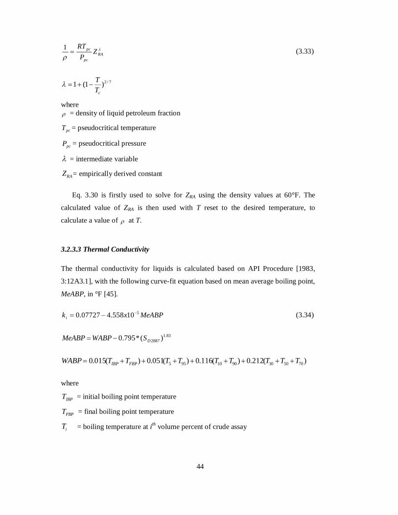
44

RApc

pc ZP

RT1 (3.33)

7/2)1(1cT

T

where = density of liquid petroleum fraction

pcT = pseudocritical temperature

pcP = pseudocritical pressure

= intermediate variable

RAZ = empirically derived constant

Eq. 3.30 is firstly used to solve for ZRA using the density values at 60°F. The

calculated value of ZRA is then used with T reset to the desired temperature, to

calculate a value of at T.

3.2.3.3 Thermal Conductivity

The thermal conductivity for liquids is calculated based on API Procedure [1983,

3:12A3.1], with the following curve-fit equation based on mean average boiling point,

MeABP, in °F [45].

MeABPxk i510558.407727.0 (3.34)

83.12887 )(*795.0 DSWABPMeABP

)(212.0)(116.0)(051.0)(015.0 7050309010955 TTTTTTTTTWABP FBPIBP

where

IBPT = initial boiling point temperature

FBPT = final boiling point temperature

iT = boiling temperature at ith volume percent of crude assay

45

3.2.3.4 Viscosity

The viscosity values for hypothetical component, i at different cut points in crude

assay are recorded at standard temperatures of 50°C and 100°C [45]. The overall

viscosity for mixture of hypothetical components at 50°C and 100°C is determined by

combining the viscosity blending number, VBN, of pseudo-components as given

below.

21.0 If )8.0(loglog47.331.2321.0 If 56

1010

ii

iiVBN

(3.35)

The VBN for the crude assay (mixture of hypothetical components), VBNT, is

determined as

Ti

n

i

Ti

Ti

n

iT

V

VBNVVBN

1

1

(3.36)

where

T = temperature of viscosity value either at 50 oC or 100 oC

VBNiT = VBN of component i at temperature T

Vi = volume percent of component i at temperature T

The viscosity of crude assay at either 50 oC or 100 oC, T , is calculated based on

equations as given.

-56 for 8.010

-56 for 21.010

VBN

VBNT

(3.37)

where

47.331.23

VBN

The viscosity values at temperatures other than 50 oC or 100 oC, VT is determined

based on ASTM D341 procedures [45]. The calculations are given as:

46

7.01010 C

D (3.38) where

)273(log)273(log)273(log

)273(log 10210110

211101

T

TTXXTXC

T1 = viscosity reference temperature at 50 oC

T2 = viscosity reference temperature at 100 oC

T = temperature at which viscosity is required.

0.2for 7.0loglog

0.2115290for 51.084.147.1exp(7.0loglog

1010

2,1010

TNTn

TnTnnTTnn

VVV.VVVX

where

VTn = viscosity at temperature Tn with n = 1 or 2

Xn = intermediate values Xn with n = 1 or 2

Based on Eqs. 3.33-3.36, the viscosities of crude oil at 50 oC and 100 oC are estimated

as given

0.2 if 0.2 if 3193.06119.0295.37487.0exp( 32

DDDDDDDVT (3.39)

3.3 Crude Preheat Train Model

The CPT model consists of seven heat exchangers from downstream of desalter till

upstream of fired heater. This section of CPT is chosen due to: i) the fouling at

upstream of desalter are mainly contributed by unsettled fine particles and minerals

which are difficult to estimate using mathematical model, ii) established fouling

models [15, 35, 36, 46] are only applicable to chemical reaction fouling, iii) chemical

reaction fouling always occurred at elevated temperatures as stated by Wilson et al.

[47] and Bott [17]. The mechanical design, physical arrangements, and operational

47

constraints of the heat exchangers are collected from an operating refinery. The

schematic diagram of CPT is shown in Fig. 3.3.

48

Figure 3.3: Layout of crude preheat train

48

49

The crude oil that is free of inorganic salts after desalter is routed through the tube

sides of E-1A~D that consists of four shells. The four-shell heat exchanger is formed

by two series of heat exchangers, E-1A/B and E-1C/D that are arranged in parallel.

After that, the heated crude oil is combined and routed through the tube side of E-2

and subsequently through the tube side of E-3. Both E-2 and E-3 are single-shell heat

exchangers. The crude oil is then routed through the shell sides of E-4A~D. E-4A~D

has the same shells arrangements as in E-1A~D. The four-shell heat exchanger

formed two series of heat exchangers, E-4A/B and E-4C/D that are arranged in

parallel. After preheated in E-4A~D, the crude oil is combined and fed to the tube side

of E-5 and later through the tube side of E-6. Both E-5 and E-6 are single-shell heat

exchangers. Finally, the crude oil is split equally to E-7A and E-7B that are arranged

in parallel. The preheated crude oil is then combined and routed through the fired

heater to heat to coil outlet temperature (COT) in preparation of separation process in

crude distillation column (CDU). The preheating mediums are the hot products and

pump-around streams of CDU at different operating conditions. Product 4 has the

highest inlet temperature, followed by Product 6, Product 3, Product 2 and Product 1.

Product 5 has the lowest inlet temperature. The design specifications of these heat

exchangers are summarized in Tables 3.1-3.4.

50

Table 3.1: Mechanical geometries of heat exchangers

Heat Transfer Area Baffle Type Shell Arrangement Tubes per shell Tube Passes Velocity, m/s m2 Series Parallel Shell Tube

1. E-1 A~D 1624 Single Segmental 2 2 91 2 0.50 0.78

2. E-2 238 Single Segmental 1 1 454 1 0.35 2.12

3. E-3 296 Single Segmental 1 1 570 1 0.10 1.70

4. E-4 A~D 544 Single Helix 2 2 99 2 1.83 0.96

5. E-5 495 Single Segmental 1 1 749 1 0.26 1.35

6. E-6 243 Single Segmental 1 1 362 1 0.34 2.89

7. E-7 A/B 295.2 Single Helix 1 2 108 1 1.91 1.20

Table 3.2: Heat Transfer details of heat exchangers

Heat Duty U Fluid (Shell)

ho (Shell)

∆P (Shell) norm/max

Fluid (Tube)

hi (Tube)

∆P (Tube) norm/max

kW W/m2 oC W/m2 oC kPa W/m2 oC kPa 1. E-1 A~D 6985 516 Product 1 1082 29/70 Crude 1034.8 18/50

2. E-2 1629 677 Product 2 714.5 14/70 Crude 2391.8 35/70

3. E-3 1409 175 Product 3 444.1 3/70 Crude 1952.4 24/70

4. E-4 A~D 3280 496 Crude 877.3 60/70 Product 4 944.4 59/70

5. E-5 2854 544 Product 5 500.8 9/70 Crude 1659.4 18/50

6. E-6 6839 699 Product 6 1424.8 14/70 Crude 2868 63/70

7. E-7 A/B 5858 555 Crude 786.9 30/30 Product 4 1334.6 19/70

Table 50

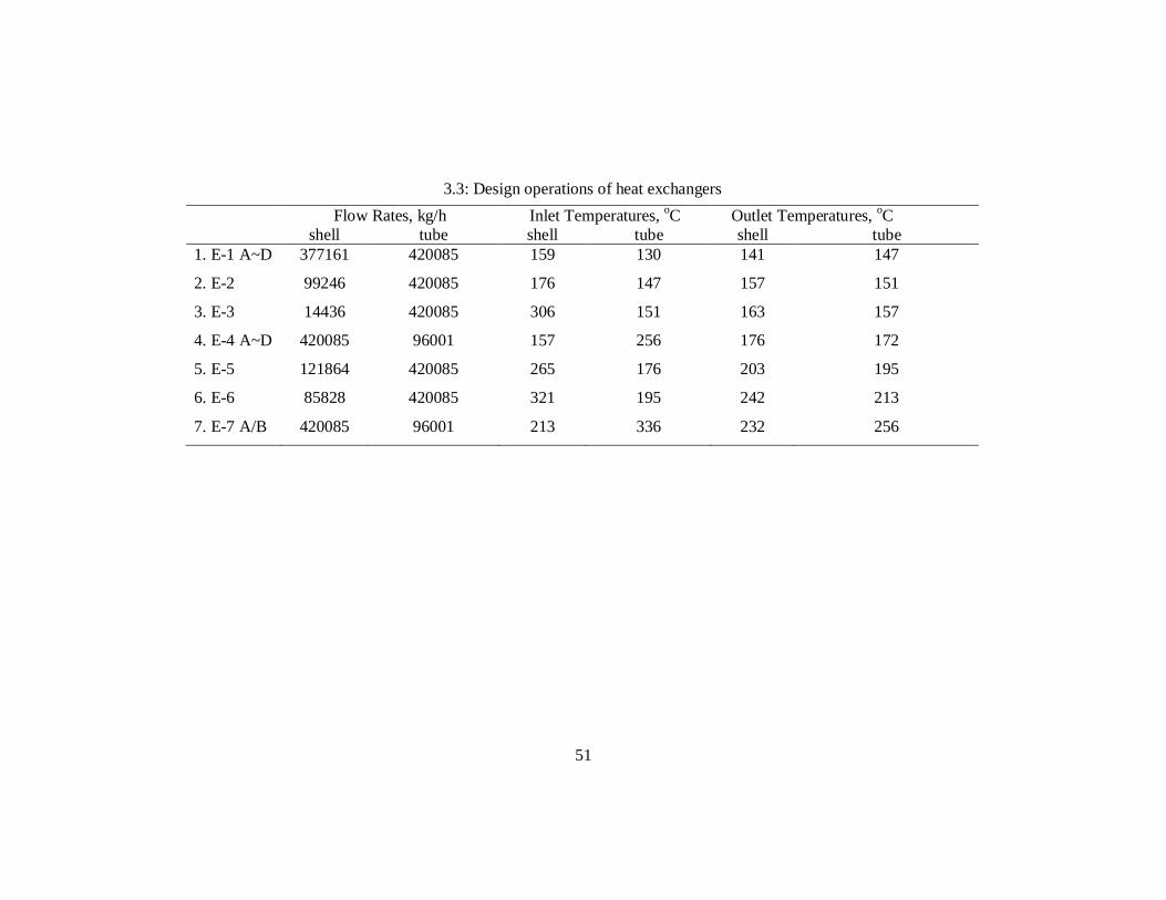
51

3.3: Design operations of heat exchangers Flow Rates, kg/h Inlet Temperatures, oC Outlet Temperatures, oC shell tube shell tube shell tube

1. E-1 A~D 377161 420085 159 130 141 147

2. E-2 99246 420085 176 147 157 151

3. E-3 14436 420085 306 151 163 157

4. E-4 A~D 420085 96001 157 256 176 172

5. E-5 121864 420085 265 176 203 195

6. E-6 85828 420085 321 195 242 213

7. E-7 A/B 420085 96001 213 336 232 256

51

52

Table 3.4: Fluid physical properties at design operating conditions , kg/m3 Cp, kJ/kgK , cP k, W/mK shell tube shell tube shell tube shell tube

1. E-1 A~D 637 716 2.67 2.49 0.202 0.535 0.099 0.093

2. E-2 668 702 2.71 2.57 0.250 0.459 0.090 0.089

3. E-3 678 698 3.24 2.59 0.360 0.443 0.069 0.088

4. E-4 A~D 693 788 2.62 2.76 0.348 1.808 0.087 0.077

5. E-5 640 675 3.05 2.71 0.201 0.348 0.076 0.086

6. E-6 642 656 3.31 2.80 0.227 0.289 0.064 0.089

7. E-7 A/B 637 737 2.89 3.08 0.258 0.377 0.095 0.068

52

53

3.3.1 Mathematical Model

The mathematical model of crude preheat train considers serial and parallel

arrangements of heat exchangers. The major parameters are fluid temperatures, fluid

flow rates and fluid bulk properties (heat capacity ( pC ), density ( ), thermal

conductivity (k) and viscosity ( )). Each of the n heat exchangers is characterized by

heat exchange area ( A ), tube side heat transfer coefficient (hi), shell side heat

transfer coefficient (ho), and fouling resistance (Rf). These information forms a set of

input data to the CPT model.

The heat transfer rate for nth heat exchanger is given by

nnnnn LMTDFAUQ . (3.40)

Assuming no energy loss, an energy balance on cold and hot streams of nth heat

exchanger can be written as

)( ,,,cinn

coutncpcc TTCMQ (3.41)

)( ,,,houtn

hinnhphh TTCMQ (3.42)

hcn QQQ (3.43)

Subscripts c and h refer to cold and hot streams, respectively. The overall heat

transfer performance, Q of the CPT model is given as

n

iiQQ

1 (3.44)

The heat transfer coefficient value from the design data sheet at the design

operating conditions is considered to be the base value to determine the actual heat

transfer coefficient, ho. In the calculation, correction factors ( lb JJ , ) that are related to

mechanical geometries of the heat exchangers are not considered. Correction factor,

rJ , is assumed equal to 1 based on the assumption that only turbulent flow exist.

The changes in actual heat transfer coefficients are only due to the variations in

54

the physical properties of the fluids and operating conditions. Therefore the heat

transfer coefficients can be calculated as a correction from the design operating

conditions and properties. The ratio of actual shell side heat transfer coefficient and

shell side design heat transfer coefficients (ho/ho,d) for single segmental baffle is given

by :

3/23/2

,

1.165.0

,

ddp

p

ddddo

o

kk

CC

vv

hh

(3.45)

Based on Colburn equation, the ratio of actual tube side heat transfer coefficient

and design tube side heat transfer coefficient (hi/hi,d) is given by:

6.04.0

,

4.08.0

,

ddp

p

ddddi

i

kk

CC

vv

hh

(3.46)

The ratio of actual shell side heat transfer coefficient and shell side design heat

transfer coefficient (ho/ho,d) for single helix baffle is given by :

3/23/1

,

4.07.0

,

ddp

p

ddddo

o

kk

CC

vv

hh

(3.47)

3.3.2 Fouling Modeling

The fouling resistance, Rf , is given by [42],

cleantf UU

R 11 (3.48)

where

tU = overall heat transfer coefficient at time t

cleanU = overall heat transfer coefficient under clean condition

Fouling model as proposed by Panchal et al. [35] is used to determine the fouling

rates of heat exchangers and is given by

55

Wf

f

RTE

dtdR

expPrRe 33.0 (3.49)

where

2

21 vfw

42.0Re264.00035.0 f for turbulent flow

)(55.0 bwbf TTTT

= fouling deposition constant

= fouling removal constant

E = activation energy of crude

bT = bulk temperature of heat exchanger

wT = wall temperature of heat exchanger

fT = film temperature of heat exchanger

w = shear stress

= constant

A value of 0.88 for is recommended [15] to determine an effective film

thickness for the thermal-boundary layer. The equation is then expressed as

4/1

233.088.0

Re20791.0expPrRe v

RTE

dtdR

f

f (3.50)

Integrating the Eq. 3.48, the cumulative Rf for nth heat exchanger is given by

dtvRT

ERRf

t

tff

i

iii

4/1

233.088.0

Re0.03955expPrRe

1

1

(3.51)

In this study, fouling model parameters are extracted from historical data based on

the assumptions that: i) fouling mechanisms in the selected case study involved

56

chemical reaction fouling, and ii) the fouling happens only at tube side of heat

exchangers in CPT.

Rf for heat exchangers in CPT are calculated from the historical data of an

operating refinery. Then, the fouling rate, dt

dR f , is determined as the slope of the

graph, Rf versus time for the selected time frames. The assumptions for selection of

time frames are: (i) same crude oil blend is processed throughout the selected time

frame, (ii) drop in Rf profile due to mechanical cleaning or hot melting of heat

exchangers will not be included, and (iii) outliers of operating parameters will not be

included. w for each heat exchanger is calculated based on average values of

calculated Re, Pr and Tf during the selected duration. dt

dR f versus w is then plotted

for each heat exchanger to determine that is equivalent to the slope of the graph.

Then the and E are solved simultaneously using Microsoft Excel for minimum root

mean square error, RMSE, by comparing the differences of calculated dt

dR f versus

actual dt

dR f derived from actual operating data.

For E-1A~D, E-3 and E-5 that have approximately the same shear stress, the

activation energy, E, of the crude oil is computed as average value of the results of E-

1A~D, E-3 and E-5.

For E-2 and E-6 that have different w , a different approach is used to determine

and . The average E that is estimated from simultaneous convergence of E-

1A~D, E-3 and E-5 is assumed valid for E-2 and E-6 as fouling is assumed to be

occurred at crude oil side. Then, and are solved to determine the minimum

RMSE, by comparing the differences of calculated dt

dR f versus actual dt

dR f that

derived from actual operating data.

For E-4A~D and E-7A/B that have different heat transfer medium (Product 4)

through the tube side, the fouling model parameters, , and E, are solved

57

simultaneously using Microsoft Excel for minimum root mean square error, RMSE,

by comparing the differences of calculated dt

dR f versus actual dt

dR f derived from

actual operating data.

3.4 Summary

This chapter presented the development of CPT simulation model in detail. The

governing equations, estimation of overall heat transfer coefficients and established

first principle thermodynamic correlations for physical properties used in the

mathematical model were discussed. The mechanical arrangements, geometries and

design specifications of the CPT model were presented. Lastly, the fouling model and

the approaches to estimate fouling model parameters were also presented.

58

59

CHAPTER 4

SIMULATION STUDIES

4.1 Introduction

A good understanding of effects of fouling on individual heat exchangers in a heat

exchanger network (HEN) is important to prioritize the cleaning process in

minimizing the operating cost. The analysis can be performed by studying the heat

transfer interactions between the heat exchangers in terms of physical arrangements,

positions, thermal designs and fouling.

In this section, a simulation study was performed using a mathematical model of

crude preheat train (CPT) to analyze the effects of fouling on each heat exchanger and

overall CPT. Semi-empirical fouling model is used to estimate the fouling behavior,

with the model parameters extracted from historical data collected from a refinery that

processes sweet crude oil. The details and results of simulation study are discussed in

this section.

4.2 Simulation of the CPT Under Fouled Conditions

Simulation of CPT under fouled conditions comprises three essential elements, which

are; i) input data (Temperature, pressure and mass flow) to the CPT model, ii) fouling

parameters (deposition constant, 훼, and removal constant, 훾) for each heat exchanger,

and iii) mathematical model of CPT under Petro-SIM™ environment. Details of input

data and fouling parameters are discussed in this section. The details of CPT

mathematical model are discussed in Section 3.3.

60

4.2.1 Input Data

The input data to the CPT model was extracted from the historical operating data

collected from a refinery which processes sweet crude oils. In this simulation analysis,

the operating data for the process inlet conditions to the simulation model are

summarized in Table 4.1. These input data are kept constant throughout the

simulation period. Product streams 1-6 are mainly the products from crude distillation

column (CDU) that were routed through different heat exchangers in the CPT to

preheat crude A. The pressure drop for all the heat exchangers in the CPT are

assumed at normal operating conditions, as indicated in Table 4.1 and it is assumed

that the increase in pressure drops in each heat exchanger due to fouling does not

affect the fluid flow hydraulics. The heat transfer details of the heat exchangers are

listed in Table 4.2. Table 4.3 summarizes the physical properties of fluids at clean

operating conditions.

Table 4.1: The input operating data for the simulation model

Inlet Inlet Temperature Inlet Pressure Flow Rate

Stream oC kPa kg/h

1 Product 1 174.74 885.9 257873

2 Product 2 208.74 1425 38856

3 Product 3 265.94 268 15051

4 Product 4 287.39 1259 81546

5 Product 5 176.27 748.6 106032

6 Product 6 324.11 513.2 108440

7 Crude A 118.54 2359 418233

61

Table 4.2: Heat transfer details of heat exchangers

Heat Duty U Fluid (Shell)

ho (Shell)

∆P (Shell) norm

Fluid (Tube)

hi (Tube)

∆P (Tube) norm

kW W/m2 oC W/m2 oC kPa W/m2 oC kPa

1. E-1 A~D 6985 516 Product 1 1082 29 Crude 1034.8 18

2. E-2 1629 677 Product 2 714.5 14 Crude 2391.8 35

3. E-3 1409 175 Product 3 444.1 3 Crude 1952.4 24

4. E-4 A~D 3280 496 Crude 877.3 60 Product 4 944.4 59

5. E-5 2854 544 Product 5 500.8 9 Crude 1659.4 18

6. E-6 6839 699 Product 6 1424.8 14 Crude 2868 63

7. E-7 A/B 5858 555 Crude 786.9 30 Product 4 1334.6 19

61

62

Table 4.3: Fluid physical properties at clean operating conditions

kg/m3

Cp kJ/kgK

cP

K W/mK

shell tube shell tube shell tube shell tube

1. E-1 A~D 637 716 2.67 2.49 0.202 0.535 0.099 0.093

2. E-2 668 702 2.71 2.57 0.250 0.459 0.090 0.089

3. E-3 678 698 3.24 2.59 0.360 0.443 0.069 0.088

4. E-4 A~D 693 788 2.62 2.76 0.348 1.808 0.087 0.077

5. E-5 640 675 3.05 2.71 0.201 0.348 0.076 0.086

6. E-6 642 656 3.31 2.80 0.227 0.289 0.064 0.089

7. E-7 A/B 637 737 2.89 3.08 0.258 0.377 0.095 0.068

62

63

4.2.2 Fouling Parameters

The fouling model proposed by Panchal et al. [35] is chosen to describe the fouling

rates of heat exchangers. The fouling rates depend on the operating conditions across

the CPT. The fouling model is given by

Wf

f

RTE

dtdR

expPrRe 33.0 (3.24)

The fouling model parameters (deposition constant, , and removal constant, )

are estimated from historical data as discussed in Section 3.3.2. These fouling

parameters for all the heat exchangers are summarized in Table 4.4.

Table 4.4: Fouling model parameters for heat exchangers in the CPT based on actual

operating data.

Heat Exchangers

Deposition constant,

Removal constant,

Activation Energy, E, kJ/mol

1 E-1A~D 1.031E+05 1.227E-05 39.783

2 E-2 1.200E+06 5.630E-05 39.783

3 E-3 1.031E+05 1.227E-05 39.783

4 E-4A~D 1.000E+07 1.009E-04 52.515

5 E-5 1.031E+05 1.227E-05 39.783

6 E-6 8.860E+05 7.520E-05 39.783

7 E-7A/B 1.000E+07 1.009E-04 52.515

The fouling model parameters were extracted based on assumptions that fouling

of heat exchangers in CPT is only occurring at tube side. As indicated in Table 4.4, all

the heat exchangers in the CPT have unique combinations of and . E-1A~D, E-3,

and E-5 have the same fouling model parameters as these heat exchangers process the

same heat transfer fluid at tube side. E-2 and E-6 have different fouling parameters

due to different shear stress although its tube side heat transfer fluid is crude oil. E-

4A~D and E-7A/B have the same fouling model parameters as the same heat transfer

fluid flows through the tube side. As discussed by Panchal et al. [48], fouling model

parameters should be consistent across the HEN that shared the same heat transfer

medium at tube side. In other words, only chemical reaction fouling is assumed in

64

Panchal’s case study. Similar approach is used in this study as all the fouling model

parameters were extracted from historical data collected from refinery, in which the

fouling is assumed solely contributed by chemical reaction fouling.

Activation energy, E, for the crude oil that flows through the tube side of E-

1A~D, E-2, E-3, E-5 and E-6 have been estimated to be 39.783 kJ/mol, while the E

for Product 4 that flows through the tube side of E-4A~D and E-7A/B was 52.515

kJ/mol. All these ranges of E are within reported ranges of activation energy.

Crittenden et al. [49] reported the E for crude oils in the range of 20 and 55 kJ/mol.

4.3 Results and Discussion

The CPT model was simulated for a period of 300 days. Throughout the simulation

period, the changes in physical properties such as density, heat capacity, viscosity and

thermal conductivity of crude oil and preheating mediums for intermediate streams of

each heat exchanger were determined by Petro-SIM™ software. Then, the overall

heat transfer coefficient is determined by

oo

w

i

oo

i

io

ii

o

hR

kddd

dRd

hdd

U1

2

ln1

(3.7)

The shell side heat transfer coefficient, ho, was calculated using Bell-Delaware

method for vertical segmental baffles and Peng’s method for continuous helical

baffles while the tube side heat transfer coefficient, hi, were calculated using Colburn

method, as explained in Chapter 3, Section 3.2.2.1. Fouling model for each heat

exchanger in the CPT was then used to compute the fouling resistance for each day of

the simulation period. The intermediate operating temperatures of heat exchanger

vary due to the incremental fouling resistance in each heat exchanger estimated by the

fouling model. The fouling resistances for all the heat exchangers are shown in Fig.

4.1.

65

Figure 4.1: Fouling resistances determined for all the heat exchangers.

It is observed that the fouling rates are high for some heat exchangers while it is

low for other heat exchangers. The two variables that are responsible for different

fouling rates in different heat exchangers are the fluid velocity and the wall/film

temperature. These two operating parameters vary across the heat exchangers in the

CPT depending on the mechanical geometries and operating conditions of the heat

exchangers. The velocity and film temperature data for all the heat exchangers in the

CPT are summarized in Table 4.5.These two operating parameters vary across the

heat exchangers in

0

0.005

0.01

0.015

0.02

0.025

0.03

0.035

0.04

0.045

0.05

0 50 100 150 200 250 300

Foul

ing

Res

istan

ce, m

2 K/W

Days

E1A~D

E-2

E-3

E-4A~D

E-5

E-6

E-7A/B

66

Table 4.5: Velocity and wall/film temperatures for heat exchangers in the CPT based

on design operating data

Heat Exchangers

velocity, 푣 Wall/film temperature, K

1 E-1A~D 0.708 406.5 2 E-2 2.145 417.7 3 E-3 1.521 423.6 4 E-4A~D 0.467 492.8 5 E-5 1.368 462.6 6 E-6 2.953 490.0 7 E-7A/B 1.290 554.8

Refering to Eq. 3.5, the deposition term is inversely proportional to 푣 . and

directly proportional to the Arrhenius term, exp − , while the removal term is

directly proportional to 푣 . .

Referring to Table 4.5, the effect of Tf is more dominant as compared to effect of

v. Heat exchangers E6 and E-7A/B that operates at the highest Tf have the highest

fouling rates. E-1A~D and E-4A~D have relatively lower fouling rates as compared to

E6 and E-7A/B. E-3 and E-5 have approximately the same fouling rates, which is

lower than E-1A~D and E-4A~D. Heat exchanger E-2 has the lowest fouling rate

throughout the simulation period as its high fluid velocity slow down the fouling

process. It is observed that the fouling rate in E-2 is asymptotic. Starting from 60th to

110th day, lower fouling rates have been predicted for E-2.

67

Figure 4.2: UA values determined for all the heat exchangers.

The overall heat transfer coefficients for all the heat exchangers were calculated

for every day based on the corresponding fouling resistances. The UA values for all

the heat exchangers are shown in Fig. 4.2. It is observed from Fig. 4.2 that the

decrease in UA values correspond to the fouling rates in the respective heat

exchanger. It is observed from Fig. 4.2 that the UA values drop significantly in the

first few days of simulation period and reach almost constant values on the longer run.

It may be noted that although the Rf values were increasing linearly, the UA values

asymptotically reached a constant value.

0

50

100

150

200

250

300

0 50 100 150 200 250 300

UA

, kW

/C

Days

E1A~D

E-2

E-3

E-4A~D

E-5

E-6

E-7A/B

68

Figure 4.3: Heat duty values determined for all the heat exchangers.

Fig. 4.3 shows the variations in the heat duty in individual heat exchangers due to

fouling during the simulation period. It is observed that heat duties are decreasing for

most of the heat exchangers in the CPT except E-7A/B, E-3, E-4A~D and E-5. The

decrease of heat duties for most of the heat exchangers in the CPT are due to fouling.

Higher heat transfer loss is indicated on E-6 (10,003kW) and followed by E-1

(6,666kW). A slight decrease of heat duty is observed in E-2 (139kW). It is observed

that in some heat exchangers, e.g. E4-A~D, the heat duty initially increase despite of

the fouling and decreased UA values. This is mainly due to the increase in the

approach temperatures that resulted in higher LMTD values.

0

2000

4000

6000

8000

10000

12000

0 50 100 150 200 250 300

Hea

t Dut

y, k

W

Days

E1A~D

E-2

E-3

E-4A~D

E-5

E-6

E-7A/B

69

Figure 4.4: Heat transfer efficiency determined for all the heat exchangers.

Fig. 4.4 shows the heat transfer efficiency in individual heat exchangers

undergoing fouling during the simulation period. As observed in Fig. 4.4, heat transfer

efficiency of most of the heat exchangers dropped due to fouling in asymptotic

manner except E-4A~D, E-5 and E-3. Heat exchanger E-6 has the fastest decreasing

rate of heat transfer efficiency as it has one of the highest fouling rates as indicated in

Fig. 4.1. The high fouling rate caused its heat transfer efficiency to drop to

approximately 20% in the first 20 days. The heat transfer efficiency of E-2 decrease

for the first 120 and increased slightly till the end of the simulation period. During the

first 120 days, the fouling in E-1 caused a drop in the heat transfer efficiency of E-1

and E-2. This observation is aligned with the fouling characteristics of E-1 and E-2.

At the end of 120 days, heat transfer efficiency of E-1 dropped to approximately 25%,

and this caused an increase in the inlet temperature of the process fluid to E-2. With

constant inlet temperature of the heating medium to E-2, the approach temperature

increased leading to higher LMTD values. Small variation in the heat transfer

efficiency was observed in E-2, whereas its heat transfer efficiency remained around

90-110 % despite the increase in the fouling resistance throughout the simulation

period.

0

50

100

150

200

250

0 50 100 150 200 250 300

Hea

t Tra

nsfe

r Ef

ficie

ncy,

%

Days

E1A~D

E-2

E-3

E-4A~D

E-5

E-6

E-7A/B

70

Heat transfer efficiency of E-4A~D increased slightly during the first 50 days and

dropped after that. The heat transfer performance of E-5 improved drastically up to

200% within the first 40 simulation days. As compared to E-5, the heat transfer

performance of E-4A~D improved only up to 150% within the first 75 days.

As observed in Fig. 4.2, fouling of CPT have the least impact to the UA values of

E-7A/B and E-4A~D. The heat transfer performance of E-4A~D is highly dependent

on E-7A/B as preheating medium of E-4A~D is routed from the outlets of E-7A/B. As

indicated in Fig. 4.4, an increase in heat transfer efficiency is observed in E-7A/B

during the initial 10 days due to the combined effect of low fouling and high LMTD

value. Low fouling will contribute to higher U while high LMTD will results a higher

heat transfer across the heat exchanger. In the same duration, the heat transfer

performance of E-4A~D was observed to decrease as the inlet temperature of

preheating medium from the outlets of E-7A/B are hotter, which reduces the LMTD

for E-4A~D. Hence, less duty transfer is observed for E-4A~D. Colder crude oil at

outlets of E-4A~D increases the LMTD of E-5 and hence improved the heat transfer

by 37%. This is supported by Fig. 4.4 that indicated the heat transfer efficiency of E-5

increased to 200% during this period.

After 10 days, higher fouling in E-7A/B has resulted in lower LMTD values, and

hence reduced the heat transfer performance of E-7A/B. This can be observed from

Fig. 4.3, which the heat transfer for E-7A/B is increasing at initial stage of the

simulation time, and decrease after few days. Due to less heat exchange in E-7A/B

while the same operating temperature and flow of preheating medium are maintained,

hotter preheating medium is routed to E-4A~D. The hotter preheating medium

increased the LMTD and compensated the decrease of U of E-4A~D. This LMTD

effect increased the heat transfer duty of E-4A~D by 1.71 MW, which is

approximately equivalent to a performance improvement of 44%.

Comparison of reduction in heat duties in the individual heat exchangers with the

total heat duty loss due to fouling shows that E-6 and E-1A~D results in the highest

fouling impact to the total duty loss in the CPT. As observed from Fig. 4.3, E-6 and

E-1A~D contributed to 30.9% and 20.6% of the total heat loss of the CPT

respectively due to effects of fouling and LMTD.

71

High fouling of E-7A/B has increased the crude oil outlet temperature of E-4A~D.

This hence decreases the heat transfer driving force for the heat exchangers at the

downstream of CPT. E-6 has the most drastic decrease in heat transfer as it has the

highest fouling tendency among all the heat exchangers in the CPT as observed in

Fig. 4.2. Lowest LMTD effect is observed in E-1A~D. All the operating temperatures

and flows to this heat exchanger is fixed as this is the first heat exchanger of the CPT.

The changes of LMTD values are merely due to changes of intermediate outlet

temperatures of E-1A to E-1B that are arranged in series. Similar effect is observed on

E-1C and E-1D.

The total heat duty for the CPT for the simulation period is shown in Figure 4.5.

The total heat recovery of the CPT had dropped by 23.99 MW from 32.33 MW to

8.33 MW at the end of 300 simulation days due to fouling.

Figure 4.5: Total heat transfer value determined for all the heat exchangers.

The crude oil from the last heat exchanger in the CPT is pumped into the fired

heater to further heat the crude oil to the operating feed temperature of CDU. The

inlet temperature to the fired heater is called the coil inlet temperature (CIT).

5

10

15

20

25

30

35

0 50 100 150 200 250 300

Tota

l Hea

t Dut

y, k

W

Days

72

Figure 4.6: CIT values determined for all the heat exchangers.

Fig. 4.6 shows that coil inlet temperature (CIT) dropped by 76.93 °C from 224.3

to 147.39 °C at the end of 300 days. Based on the calculation for a preheat train

processing similar throughput as provided by refinery, the cost of fuel gas is

approximately RM11.30 to generate one Giga Joule of heating energy in fired heater

as reported from an operating refinery. Thus, the reduction in CIT results in additional

fuel cost equivalent to RM 8.72 mil in one year.

140

150

160

170

180

190

200

210

220

230

0 50 100 150 200 250 300

Coi

l Inl

et T

empe

ratu

re, o C

Days

73

4.4 Summary

This chapter presented a heat transfer analysis of the seven units of heat exchangers

after desalter in the CPT for a crude distillation unit in 300 days. Same operating

conditions were input to inlet process boundaries of the CPT model under Petro-

SIM™ environment throughout the simulation duration. Fouling model as proposed

by Panchal et. al. [15] was used to estimate the fouling rates of heat exchanger, with

its fouling parameters were estimated from historical operating data from an operating

refinery.

Different heat transfer performances of heat exchangers are observed during the

simulation period due to fouling. Heat transfer performance dropped for some of the

heat exchangers and increased for other heat exchangers. Drop in heat transfer

performances are observed on E-6 and followed by E-1 and E-2 due to fouling.

Improvement on heat transfer performances are observed on E-7A/B, E-3, E-4A~D

and E-5. These improvements are mainly contributed by LMTD effects in CPT.

The analysis indicated that position of heat exchangers has essential roles in heat

transfer performance in the CPT during fouling condition. As indicated in this

simulation study, fouling of first heat exchanger of the CPT will have higher impact

to overall heat transfer performance of the CPT. In this study, it is observed that even

at consistent increase of fouling rates, the loss of heat performance due to fouling can

be compensated by LMTD effect. To certain extent, LMTD effect will slow down

fouling effect or even increase the heat transfer performance in some of the heat

exchangers in the HEN.

74

75

CHAPTER 5

OPTIMIZATION OF CLEANING SCHEDULE

5.1 Introduction

Cleaning of heat exchangers to remove deposits due to fouling in crude preheat train

(CPT) is a normal ad-hoc operation in oil refineries. The performance of CPT is

evaluated by the plant operators solely based on operating experience. In general,

plant operators have the views that the heat exchangers should be cleaned when the

CPT exceeds the operational limits. These operational limits are abnormally high

pressure drops across the heat exchangers, insufficient firing in the fired furnace to

achieve targeted coil outlet temperature (COT) at full plant throughput, and

production schedule from planning department. The ad-hoc and improper planning of

cleaning schedule of CPT will affect the productions of the refinery and hence result

in economic losses. This chapter discusses the formulation and solution of an

optimization problem for the cleaning schedule of CPT.

A base case for the cleaning of heat exchangers has been developed based on the

maximum allowable fouling resistances in the heat exchangers that correspond to

maximum allowable pressure drops across the heat exchangers. Operations beyond

the maximum allowable pressure drops lead to reduction in the plant throughput to

overcome the high pressure drops by the feeding pumps.

This ad-hoc cleaning generally results in: i) higher economic loss due to

unrecovered energy, ii) unplanned reduced throughputs with high penalties, and iii)

operating difficulties. An optimal cleaning schedule taking into account all the factors

will result in a minimal operating cost with less disruption in the plant operations.

76

5.2 Formulation of Optimization Problem

The model developed to describe the CPT, as explained in Section 3.3, is used in the

study of optimization of cleaning schedule of the CPT.

5.2.1 Objective Function

An optimal cleaning schedule of the CPT depends on the following costs:

i. Unrecovered energy cost: The unrecovered energy is the difference between

the heat transfer duties at fouled conditions and the corresponding clean

conditions in the heat exchangers in the CPT.

ii. Cleaning costs: The cleaning costs of heat exchangers involve the costs

associated with the initial preparations for heat exchanger isolation,

mechanical/chemical cleaning and reinstallation of the heat exchangers. The

cleaning costs generally depend on the size of the heat exchangers.

Based on the above costs, an objective function is formulated as shown in Eq. 5.1.

p E

n,t

t

t

N

n tncltncleanntnEyyCQQyCJ

1 1 ,,, )1(),( min (5.1)

where tp = total period of operation

t = time, day

n = nth heat exchanger

C E = cost of energy per day

cleannQ , = heat transfer duty under clean conditions in the nth heat exchanger

tnQ , = heat transfer duty under fouled (actual) conditions in the nth heat exchanger

clC = cost of heat exchanger cleaning per day

NE = the total number of heat exchangers in the CPT

tny , = the cleaning status of nth heat exchanger unit at time t

The cleaning status of the heat exchangers, tny , , is a binary variable, where it is

77

equal to 1 if nth heat exchanger is in service, and it is equal to 0 if it is under cleaning.

In the optimization problem of Eq. 5.1, the optimization variables are the cleaning

status of the heat exchangers. The number of optimization variables is equal to the

total optimization period in days for each heat exchanger, which is extremely large in

number. In practice, the cleaning status of any heat exchanger is equal to 1 for the

whole duration of the heat exchanger between successive cleanings. Therefore, the

cleaning status of heat exchangers can be replaced with the duration between

successive cleaning which results in a fewer number of optimization variables. In this

study, the duration between cleanings, ts,n, in days will be the optimization variables.

The optimization problem needs to be solved using mixed integer programming

approach to determine the optimal duration between cleanings of heat exchangers in

the CPT.

The starting day of the jth cleaning for the nth heat exchanger in the optimization

cases, is determined by

1)1(,,, nncnnsjn jtjtt (5.2)

where

nct , = cleaning duration for nth heat exchanger

nj = jth cleaning cycle of nth heat exchanger

All the heat exchangers are assumed that they can be bypassed either

independently or sharing the same bypass facility with another heat exchanger. Heat

exchangers E-1A~D, E-4A~D and E-7A/B can be bypassed independently. E-2 and E-

3 share the same bypass facility. Same bypass facility is also equipped for E-5 and E-

6. The heat exchangers that share the same bypass facility must be cleaned

simultaneously during the cleaning period regardless of the fouling condition of other

heat exchanger that shares the bypass facility.

The cleaning of the seven heat exchangers in the CPT model depends on the

arrangement of shells, i.e., either in series or in parallel. For E-1A~D and E-4A~D

that have 2 trains of heat exchangers in parallel, cleaning of one heat exchanger train

will not affect the operation of the other heat exchanger train. Heat exchanger E-7A/B

78

consists of 2 heat exchangers in parallel. Similar to cleaning cycles of E-1A~D and E-

4A~D, cleaning of one heat exchanger will not affect the operation of the other heat

exchanger. The cleaning of the second heat exchanger is performed after cleaning the

first heat exchanger.

The cleaning duration for one heat exchanger is assumed to be 5 days, based on

the industrial experience. Same cleaning duration is applied for one heat exchanger

train that consists of two heat exchangers, assuming both the heat exchangers are

cleaned simultaneously. The cleaning of second heat exchanger train is performed

after the cleaning cycle of first train. With that, the cleaning durations for E-1A~D, E-

4A~D and E-7A/B are 10 days for each cleaning. The cleaning durations for E-2, E-3,

E-5 and E-6 are 5 days for each cleaning.

The amount of supplement heating energy required to maintain coil inlet

temperature (CIT) at 225 °C was measured at the outlet of heat exchanger E-7 A/B.

The supplemented heating energy is then converted to monetary basis based on the

value of energy cost, EC , which is equivalent to RM11.30/GJ.

The cleaning costs of heat exchangers differ based on the heat transfer area,

mechanical arrangements and availability of bypass facilities. The nominal cleaning

costs for the heat exchangers in the CPT are obtained from the plant as shown in

Table 5.1.

Table 5.1: Cleaning durations and mechanical cleaning costs of heat exchangers in

CPT.

Heat Exchangers tc,n (days) niclC , (RM/day) 1. E-1A~D 10 30, 000

2. E-2 5 10, 000

3. E-3 5 10, 000

4. E-4A~D 10 20, 800

5. E-5 5 11, 800

6. E-6 5 9, 600

7. E-7A/B 10 18, 300

79

Fouling results in the formation of roughened deposits adhering to the surface of

the heat exchanger tubes. The crude oil is often passed through the tubes and the flow

area reduces as these deposits grow, increasing the flow resistance encountered within

the exchanger and ultimately the network. There are occasions when the flow

resistance becomes so high that the operators have to reduce throughput. These flow

resistances can be measured based on pressure drops of the heat exchangers and these

parameters are crucial to be monitored in this optimization study. In general, the

pressure drops in the heat exchangers are directly proportional to the corresponding

fouling resistances [22]. An increase in the fouling deposition in the heat exchangers

increases the pressure drop, which reduces the throughput across the heat exchangers.

Nevertheless, changes in pressure drop for each heat exchanger due to the

variations in throughput are not simulated in this optimization study. Alternatively,

the highest allowable fouling resistances for heat exchangers extracted from historical

data are used as one of the constraints. The fouling resistance constraints for all the

heat exchanger are indicated in Table 5.2.

Table 5.2: Maximum allowable fouling resistances for the heat exchangers in CPT

Heat Exchanger Fouling Resistance W/m2K

1. E-1A~D 2.30E-02

2. E-2 1.06E-02

3. E-3 1.30E-02

4. E-4A~D 1.44E-02

5. E-5 1.49E-02

6. E-6 2.30E-02

7. E-7A/B 1.80E-02

5.2.2 Constant Fouling Rates

Different types of crude oils were blended and preheated in the CPT during the

period for which the historical operating data was collected from the plant. Mostly, a

crude oil blend is only processed for less than two weeks and none of the crude oil

blends were repeatedly processed for more than three times in the two years duration.

80

The fouling rates of each heat exchanger in the CPT determined from the historical

data were plotted in Figs. 5.1-5.7. Equal fouling rate is assumed in all the shells of a

multi-shell heat exchanger. It is observed from Figs. 5.1-5.7 that the fouling

resistances increased nearly linearly in all the heat exchangers. The fouling rates at

different points in time in any heat exchanger are almost the same even though

various types of crude oil blends were processed at different times. Thus, it is

assumed in this optimization study that all the heat exchangers have constant linear

fouling rates. The observed fluctuations in the values of fouling rates were mainly due

to variations in the crude oil blends and also the velocity due to the variations in the

throughput. The constant fouling rates for heat exchangers in the CPT are summarized

in Table 5.3.

Figure 5.1: Observed fouling resistances for heat exchanger E-1A~D

0.00E+00

5.00E-03

1.00E-02

1.50E-02

2.00E-02

2.50E-02

0 200 400 600 800

Foul

ing

Res

istan

ce, m

2 K/W

Time, Day

81

Figure 5.2: Observed fouling resistances for heat exchanger E-2.

Figure 5.3: Observed fouling resistances for heat exchanger E-3.

0.00E+00

2.00E-03

4.00E-03

6.00E-03

8.00E-03

1.00E-02

1.20E-02

1.40E-02

1.60E-02

1.80E-02

2.00E-02

0 200 400 600 800

Foul

ing

Res

istan

ce, m

2 K/W

Time, Day

0.00E+00

2.00E-03

4.00E-03

6.00E-03

8.00E-03

1.00E-02

1.20E-02

1.40E-02

1.60E-02

1.80E-02

2.00E-02

0 200 400 600 800

Foul

ing

Res

istan

ce, m

2 K/W

Time, Day

82

Figure 5.4: Observed fouling resistances for heat exchanger E-4A~D.

Figure 5.5: Observed fouling resistances for heat exchanger E-5.

-5.00E-03

0.00E+00

5.00E-03

1.00E-02

1.50E-02

2.00E-02

2.50E-02

3.00E-02

3.50E-02

4.00E-02

4.50E-02

0 200 400 600 800

Foul

ing

Res

istan

ce, m

2 K/W

Time, Day

0.00E+00

2.00E-03

4.00E-03

6.00E-03

8.00E-03

1.00E-02

1.20E-02

1.40E-02

1.60E-02

0 200 400 600 800

Foul

ing

Res

istan

ce, m

2 K/W

Time, Day

83

Figure 5.6: Observed fouling resistances for heat exchanger E-6.

Figure 5.7: Observed fouling resistances for heat exchanger E-7A/B.

0.00E+00

1.00E-02

2.00E-02

3.00E-02

4.00E-02

5.00E-02

6.00E-02

0 200 400 600 800

Foul

ing

Res

istan

ce, m

2 K/W

Time, Day

0.00E+00

2.00E-03

4.00E-03

6.00E-03

8.00E-03

1.00E-02

1.20E-02

1.40E-02

1.60E-02

1.80E-02

0 200 400 600 800

Foul

ing

Res

istan

ce, m

2 K/W

Time, Day

84

Table 5.3: Constant fouling rates for heat exchangers in the CPT

Heat Exchanger

dRf/dt (W/m2K)/day

1. E-1A~D 9.69E-05

2. E-2 4.02E-05

3. E-3 5.02E-05

4. E-4A~D 5.26E-05

5. E-5 6.05E-05

6. E-6 2.10E-04

7. E-7A/B 1.54E-04

The fouling rate normally increases with heat exchanger tube wall temperature

and reduces with surface shear. Heat exchangers E-6, E-7 A/B, and E-1A~D have the

highest fouling rates while E-5, E-4A~D and E-3 have relatively lower fouling rates.

Heat exchanger E-2 has the lowest fouling rate throughout the operating period.

During the optimisation study, the fouling resistances for the heat exchangers were

assumed to be 0.000001 W/m2K after the mechanical cleaning of the heat exchanger.

5.3 Results and Discussions

The cleaning schedule optimization for the CPT was performed for a period of two

years. The inputs to the CPT model are varied daily based on the collected historical

operating data from an operating refinery. These inputs include: i) operating

temperatures at boundary conditions, and ii) flow rates of process and preheating

fluids at the boundaries.

85

5.3.1 Base Case

A base case of cleaning schedule for the CPT was estimated based on the

assumptions: i) the heat exchangers must be cleaned when the fouling resistance of

the heat exchanger is more than the maximum allowable limit as specified in Table

5.2, and, ii) constant linear fouling rates are used to predict the fouling resistances for

each heat exchanger (as discussed in section 5.2.1). As a result, the costs of HEN for

base case are determined as shown in Table 5.4.

Table 5.4: Operating costs of heat exchangers in CPT for base case.

Description Cost, mil RM/yr

1. Total un-recovered energy 5.711

2. Total cleaning costs 1.387

Total Operating cost 7.097

Table 5.5: Durations between cleanings for heat exchangers in CPT base case.

Duration between cleanings, days Case E-1A~D E-2 E-3 E-4A~D E-5 E-6 E-7A/B Base Case 249 266 266 285 120 120 128

86

Table 5.6: Cleaning schedule of base case for 2 years of CPT operation.

M 1

M 2

M 3

M 4

M 5

M 6

M 7

M 8

M 9

M 10

M 11

M 12

E-1A~D E-2 E-3 E-4A~D E-5 E-6 E7A~B

M 13

M 14

M 15

M 16

M 17

M 18

M 19

M 20

M 21

M 22

M 23

M 24

E-1A~D E-2 E-3 E-4A~D E-5 E-6 E7A~B

*M = month

As observed from Table 5.4, total operating cost of HEN is RM 7.097 mil/yr, in

which major portion of the cost is contributed by unrecovered energy cost, which is

RM 5.711 mil/yr (80.47% of the total operating cost). Cleaning cost of heat

exchangers is only RM 1.397 mil/yr (19.53% of the total operating cost).

The duration between cleanings for heat exchangers and estimated cleaning

schedule of base case are shown is Tables 5.5 and 5.6. As observed in Table 5.6, the

cleaning cycle for each heat exchanger under base case is not distributed evenly as

each of the heat exchanger has different maximum allowable fouling resistance limit

except for heat exchangers that shared the same bypass facility. As observed in Table

5.6, E-5 and E-6 need to be cleaned 3 times yearly, followed by E-7A/B that needs to

be cleaned 2 times in the first year and 3 times in second year of CPT operation. The

remaining heat exchangers need to be cleaned 1 time every operation year at different

intervals of duration.

87

5.3.2 Optimization Cases

The optimum cleaning schedule of CPT was obtained by minimizing the total

operating costs based on the objective function as discussed in Section 5.2.2. The

duration between cleanings is decreased based on the number of cleanings. In this

optimization problem, the duration between cleanings are fixed as in Table 5.7. This

assumption may be restrictive, but as a first attempt to solve the optimization problem

with minimum computational load, it is considered a right choice.

Table 5.7: Number of cleanings in a period of 2 years and the corresponding fixed duration between cleanings

Duration between cleanings, days Number of Cleanings

365 2

243 3

183 4

146 5

122 6

There are totally 4 different heat exchanger combinations of heat exchangers that

needed to be cleaned. These heat exchanger combinations are E-1A~D, E-2 & E-3, E-

4A~D, and E-7A~D. Based on the opinion from engineers of the refinery, the

minimum duration between cleaning must at least 120 days. Therefore, duration of

cleanings of E-5 & E-6 that shared the same bypass facility are not manipulated in

this optimization study as its duration of cleanings reach the minimum duration

between cleaning.

During the initial iteration, the duration between cleanings of the heat exchanger

combinations are maintained at the base case. Duration between cleaning more than

the base case will not be considered with the assumption that the hydraulic flow

limitations will occur at maximum fouling resistance constraint.

Table 5.8 shows the results of optimization. 24 runs were performed in 6 iterations

to determine the optimal cleaning schedule corresponding to the minimum operating

cost of CPT.

88

Table 5.8: Iteration results of optimization problem.

Duration between cleanings, days

Iterations E-1

A~D E-2 E-3 E-4

A~D E-5 E-6 E-

7A/B Additional Energy,

RM/2 years Cleaning Cost,

RM/2 years Total,

RM/2 years Iteration 1 Run1 183 266 266 285 120 120 128 10,536,671 3,708,026 14,244,696

Run2 249 243 243 285 120 120 128 10,583,302 3,828,184 14,411,486 Run3 249 266 266 243 120 120 128 10,830,765 3,503,655 14,334,420

Run4 249 266 266 285 120 120 122 10,773,340 3,777,604 14,550,944 Iteration 2 Run5 146 266 266 285 120 120 128 10,365,875 3,984,242 14,350,117

Run6 183 243 243 285 120 120 128 10,523,175 3,737,756 14,260,931 Run7 183 266 266 243 120 120 128 10,591,908 3,807,920 14,399,828 Run8 183 266 266 285 120 120 122 10,515,187 3,777,604 14,292,791

Iteration 3 Run9 146 243 243 285 120 120 128 10,308,383 4,013,973 14,322,356 Run10 183 183 183 285 120 120 128 10,410,052 3,839,145 14,249,198 Run11 183 243 243 243 120 120 128 10,366,291 3,837,651 14,203,942

Run12 183 243 243 285 120 120 122 10,492,638 3,737,756 14,230,394 Iteration 4 Run13 146 243 243 243 120 120 128 10,249,677 4,113,867 14,363,544

Run14 183 183 183 243 120 120 128 10,256,008 3,939,040 14,195,048 Run15 183 243 243 183 120 120 128 10,216,664 4,048,540 14,265,204 Run16 183 243 243 243 120 120 122 10,351,451 3,907,229 14,258,680

Iteration 5 Run17 146 183 183 243 120 120 128 10,086,829 4,215,256 14,302,086 Run18* 183 146 146 243 120 120 128 9,918,786 4,020,151 13,938,937 Run19 183 183 183 183 120 120 128 10,128,994 4,149,929 14,278,922

Run20 183 183 183 243 120 120 122 10,195,303 3,907,229 14,102,532 Iteration 6 Run21 146 146 146 243 120 120 128 10,018,850 4,296,367 14,315,217

Run22 183 122 122 243 120 120 128 10,048,152 4,141,818 14,189,970 Run23 183 146 146 183 120 120 128 10,010,616 4,231,040 14,241,656

Run24 183 146 146 243 120 120 122 10,147,978 4,089,729 14,237,707 *Optimized case 88

89

Figure 5.8: Results of Optimization Iterations

Fig. 5.8 showed the results of optimization for the 6 iterations. As compared to the

operating cost of base case, the optimum cleaning schedule reduced the operating cost

from RM 7.097 mil to RM 6.97 mil per year with a total operating cost saving of

RM127, 682 per year.

Table 5.9 indicates that the optimal cleaning schedule for heat exchangers in CPT

for 2 years of total simulation time.

7.12 7.137.10 7.10

6.97

7.09

6.85

6.9

6.95

7

7.05

7.1

7.15

Iteration 1 Iteration 2 Iteration 3 Iteration 4 Iteration 5* Iteration 6

Tota

l Ope

ratin

g C

ost,

RM

mil

/ yr

Iteration

89

90

Table 5.9: Optimized cleaning schedule for heat exchangers in CPT in 2 years total

simulation time

M 1

M 2

M 3

M 4

M 5

M 6

M 7

M 8

M 9

M 10

M 11

M 12

E-1A~D E-2 E-3 E-4A~D E-5 E-6 E7A~B

M 13

M 14

M 15

M 16

M 17

M 18

M 19

M 20

M 21

M 22

M 23

M 24

E-1A~D E-2 E-3 E-4A~D E-5 E-6 E7A~B

The result indicates that it is not necessary to clean all the heat exchangers with

higher fouling rates more frequently. Optimization study showed that E-5 and E-6

should be cleaned 3 times per year, while E-7A/B should be cleaned 2 times in the

first year and 3 times in the second year. The numbers of cleanings for these last three

heat exchangers in the CPT are matching against the fouling rates of these heat

exchangers, which E-6 has the highest fouling rates, followed by E-7A/B. As

observed from Table 5.9, E-2 and E-3 needs to be cleaned twice yearly. E-1A~D

should be cleaned twice a year. E-4A~D has the least cleaning requirement, which is

once yearly. As discussed in Chapter 4, log-mean temperature differences (LMTD)

play an important role in arresting the decrease or even improving the heat transfer

performances fouling resistance increases in the heat exchangers in CPT will e.

Besides, position of heat exchanger in CPT also influences the cleaning requirement

of heat exchangers. Hence, the number of cleanings for E-1A~D, E-2, E-3 and E-

4A~D are the balanced effects of fouling resistance, LMTD effects, position of heat

exchangers and the sharing of bypass facilities between heat exchangers. The

optimization yields a better total operating cost of CPT if E-1A~D, E-2, E3 and E-

4A~D are cleaned before their fouling resistance reaches maximum

91

allowable fouling resistance. This observation indicates that the normal operational

ad-hoc decision to clean the heat exchanger when it reaches its pressure drop

limitations might not economical for heat exchangers in CPT.

5.4 Summary

An optimization problem for the cleaning schedule of CPT was formulated and solved

for a period of two years. Minimum operating cost was achieved considering the total

unrecovered energy cost and cleaning cost of the heat exchangers. The optimization

of cleaning schedule of heat exchangers is able to achieve a total cost saving of RM

127, 682 per year. The results of optimization problem indicate that the key factors to

determine the optimum cleaning cycles are fouling rates and heat transfer interactions

between heat exchangers for each heat exchangers in CPT. As a norm, heat

exchangers with higher fouling rates should be cleaned more frequently to ensure

optimum heat transfer efficiency across the CPT. Nevertheless, the results indicate

that it is necessary for some of the heat exchangers in CPT to be cleaned before it

reaches maximum allowable fouling resistance.

92

93

CHAPTER 6

CONCLUSION AND RECOMMENDATIONS

6.1 Conclusions

A crude preheat train (CPT) was selected in this research as a case study for analysing

the effect of fouling and to determine an optimal cleaning schedule. Design and

operational data for a period of two years was collected from a refinery. Based on the

information collected, a rigorous CPT model was successfully developed under Petro-

SIM™ environment. In addition, the fouling models were also developed to describe

the fouling in the heat exchangers.

A simulation study was performed to investigate the effects of fouling on the

thermal performance of individual heat exchangers in the CPT and that of overall

CPT. The fouling resistances of the heat exchangers were estimated using semi-

empirical fouling models. Same operating conditions were input to inlet streams of

the CPT model. Heat transfer performances of heat exchangers were observed for a

period of 300 days of simulation. The heat transfer performance dropped for some of

the heat exchangers, and increased for other heat exchangers even though the fouling

was becoming more severe. The major observations/conclusions based on the

simulation study are listed below.

LMTD effects are observed in heat exchangers of the CPT. The increase and

decrease in the inlet temperatures for hot fluids and the process fluid,

respectively, to a heat exchanger due to the lower heat transfer performance in

the fouled upstream heat exchanger increases the temperature driving forces

and hence improves the heat transfer performance of heat exchanger in CPT.

Fouling of first heat exchanger in CPT contributes to the highest drop of heat

94

transfer performance of overall CPT.

Under the optimization study, an optimization problem was formulated and solved

for a period of two years to determine the cleaning schedule of CPT that have the total

minimum operating cost. Constant linear fouling rates were assumed for the heat

exchangers in CPT. A base case was developed to investigate the basic cleaning

schedule required to maintain the operation of CPT. The observations/conclusions of

the optimization study are below.

A savings of RM 127, 682 per year in operating cost.

Fouling rates, heat transfer interaction between heat exchangers, and

duration between cleanings are key factors in determining the cleaning

schedule of heat exchanges in CPT.

For certain instances, it is necessary for some of the heat exchangers to be

cleaned before it reaches maximum allowable fouling resistance

corresponding to maximum allowable pressure drop across the heat

exchanger to achieve a cleaning schedule of CPT that yields minimum

total operating cost.

6.2 Recommendations

Mixed integer programming approach was used to solve the optimization problem

based on rigorous simulation model of CPT. As the simulation of the rigorous CPT

model is computationally intensive and the number of function evaluations is quite

large, more powerful optimization algorithms like genetic algorithm can be used to

solve the optimization problem to identify the global minimum with less

computational load. The optimization variables can also be changed from the number

of cleanings in a fixed period to the duration between the cleanings which will be

more appropriate for continuous operating plants.

During the periods when a heat exchanger is taken out of service for cleaning, the

HEN configuration changes significantly and the balance of heat integration changes.

95

A systematic study to analyse the effect of changes in HEN configuration is

recommended.

The effects of hydraulic limitations are not studied thoroughly in this study. A

dynamic study can be performed to investigate the effect of hydraulic to HEN model

under fouling condition.

96

97

REFERENCES

[1]

ESDU (Engineering Sciences Data Unit), “Heat Exchanger Fouling in the Pre-

heat Train of a Crude Oil Distillation Unit,” in ESDU Intl, USA, 2000, Data

Item 00016.

[2] H. S. Muller, M. R. Malayeri and A. P. Watkinson, “Heat Exchanger Fouling;

Environment Impacts,” in Heat Transfer Engineering, UK, 2009, 773-776.

[3] K. J. Bell, and A. C. Mueller, “Wolverine Engineering Data Book II,” in

Wolverine Tube Inc, UK, 1984, 31-38.

[4] H.M. Steinhagen, “Heat Exchanger Fouling: Mitigation and Cleaning

Technologies,” in Publico Publications, Germany, 2000, 24-25.

[5] J.M. Chenoweth, “Final report of the HTRI/TEMA joint committee to review

the fouling section of the TEMA standards,” in Heat Transfer Engineering,

USA, 1990, 73–107.

[6] B. Peng, Q. W. Wang, and C. Chang, “An Experimental Study of Shell and

Tube Heat Exchanger With Continuous Helical Baffles,” in AEME, Xi’an

Jiaotong University, China, 2007.

[7] A. K. Sheikh, S.M. Zubair, M. Younas, and M.O. Boudair, “A Rish Based Heat

Exchanger Analysis Subject to Fouling Part II: Economics of Heat Exchangers

Cleaning,” in Elsevier Science Ltd, Saudi Arabia, 2000, 445-461.

[8] D. J. Kukulka, R. E. Baier, and J. C. Mollendorf, “Factors Associated with

Fouling in Process Industry,” in Heat Transfer Engineering, USA, 2004, 23–

29.

98

[9] B. D. Crittenden, S. T. Kolaczkowski, and T. Takemoto, “Use of tube Inserts

to Reduce Fouling From Crude Oils,” in AIChE Symp. Series, Atlanta, 1993,

295, 89, 300- 307.

[10] M. Markowski, “Reconstruction of a Heat Exchanger Network under

Industrial Constraints -The Case of a Crude Distillation,” in Elsevier Science

Ltd, Applied Thermal Engineering, Poland, 2000, 20:1535-1544.

[11] C. Rodriguez, and R. Smith, “Optimization of Operating Conditions for

Mitigating Fouling in Heat Exchanger Networks,” in Chemical Engineering

Research and Design Trans IChemE, 2007, UK, Part A.

[12] M. H. Panjeshahi, and N. Tahouni, “Pressure Drop Optimization in

Debottlenecking of Heat Exchanger Networks,” in Elsevier, Science Ltd,

Energy, Iran, 2008, 942-951.

[13] B. L. Yeap, “Design of Heat Exchanger Networks with Fouling Mitigation,” in

CGPS dissertation, University of Cambridge, UK, 2001, 28.

[14] D. Bouris, E. Konstantinidis, S. Balabani, D. Castiglia and G. Bergeles,

“Design of a novel, intensified heat exchanger for Reduced Fouling Rates,” in

International Journal of Heat and Mass Transfer 48, Greece, 2005, 3817–3832.

[15] W. A. Ebert, and C. B. Panchal, “Analysis of Exxon crude-oil slip stream

coking data,” in Fouling Mitigation of Industrial Heat-Exchange Equipment,

Begell House, 1995, USA, 451–460.

[16] K. Brodowicz, M. Markowski, “Calculation of Heat Exchanger Networks for

Limiting Fouling Effects in the Petrochemical Industry,” in Applied Thermal

Engineering, Elsevier Science Ltd, Poland, 2003, 23:2241–2253.

[17] T.R. Bott, “Fouling of Heat Exchanger,” in Elsevier Science B.V., USA, 2005,

7-32.

99

[18] F. Smaīli, D. K. Angadi, C. M. Hatch, O. Herbert, V. S. Vassiliadis, and D. I.

Wilson, “Optimization of Scheduling of Cleaning in Heat Exchanger Networks

Subject to Fouling: Sugar Industry Study Case,” in Trans ICheme, UK, 1999,

Vol. 77, Part C.

[19] M. C. Georgiadis, and L. G. Papageorgiou, “Optimal Energy and Cleaning

Management in Heat Exchanger Networks Under Fouling,” in Trans Icheme,

Greece, 2000, Vol 78-Part A.

[20] M. C. Georgiadis, and L. G. Papageorgiou, “Optimal Cleaning of Heat

Integrated Multipurpose Plants under Fouling Conditions,” in Elsevier,

Science Ltd, Applied Thermal Engineering, Greece, 2001, 21:1675-1697.

[21] M. Markowski, and K. Urbaniec, “Optimal Cleaning Schedule for Heat

Exchangers in a Heat Exchanger Network,” in Applied Thermal Engineering,

Poland, 2005, 25,1019-1132.

[22] S. Sanaye, and B. Niroomand, “Simulation of Heat Exchanger Network (HEN)

and Planning the Optimum Cleaning Schedule,” in Energy Conversion and

Management, Iran, 2007, No. 48,1450-1461

[23] E. M. Ishiyama, W. R. Paterson, and D. I. Wilson, “Thermal Effect of Fouling

on Heat Transfer, Pressure Drop, and Throughput in Refinery Preheat Train:

Optimization of Cleaning Schedules,” in Heat Transfer Engineering, UK, 2009,

805-814.

[24] Incropera, DeWitt, Bergman and Lavine, “Fundamentals of Heat and Mass

Transfer,” 6th Edition, Australia, 2002, Chapter 8.

[25] A. L. London, and R. A. Seban, “A Generalization of the Methods of Heat

Exchanger Analysis,” in Mechanical Engineering Department, Stanford

University, Stanford, 1942,.

[26] D. M. Smith, “Mean Temperature Difference in Crossflow,” in Engineering,

UK, 1934, 479-481; 138, 606-607

100

[27] A. C. Mueller, “Handbook of Heat Transfer,” in McGraw-Hill, New York,

1973, 35-80.

[28] O. Arsenyeva, L. Tovazhnyansky, P. Kapustenko, and G. Khavin,

“Mathematical Modeling and Optimal Design of Plate and Frame Heat

Exchangers,” in Chemical Engineering Transactions, Ukraine, 2009, volume

18.

[29] M. A. S. Jeronimo, L. F. Melo, A. S. Braga, P. J. B. F. Ferreira, and C.

Martins, “Monitoring the Thermal efficiency of Fouled Heat Exchangers: A

Simplified Method,” in Elservier, Science Ltd, Experimental Thermal and Fluid

Science, Portugal, 1997, 14:455-463.

[30] B. D. Critenden, Kolaczkowski, and I. L. Downey, “Fouling of Crude Preheat

Exchangers,” in Trans. IChemE, UK, 1992, Vol 79: Part A, pp. 547-557.

[31] M. Srinivasan and A. P. Watkinson, “Fouling of some Canadian Crude Oils,”

in Heat Transfer Eng., Canada, 2005, vol. 26(1), pp. 7-14.

[32] D. Q. Kern, and R. E. Seaton, “A Theoretical Analysis of Thermal Surface

Fouling,” in Br Chem Eng, Germany, 1959, 258-262

[33] J. Aminian, and S. Shahhosseini, “Evaluation of ANN Modeling for Prediction

of Crude oil Fouling Behavior,” in Applied Thermal Engineering, Elsevier

Science Ltd, Iran, 2008, No. 28- 668-674.

[34] V. R. Radhakrishnan, M. Ramasamy, H. Zabiri, V. D. Thanh, N. M. Tahir, H.

Mukhtar, M. R. Hamdi, and N. Ramli, “Heat Exchanger Fouling Model and

Preventive Maintenance Scheduling Tool,” in Applied Thermal Engineering,

Malaysia, 2007, No. 27-2791-2802.

[35] C. B. Panchal, W. C. Kuru, C. F. Liao, W. A. Ebert, and J. W. Palen,

“Threshold Conditions for Crude Oil Fouling, Proc. Understanding Heat

Exchanger Fouling and Its Mitigation,” in Engineering Foundation Conf.,

Italy, 1997.

101

[36] G. T. Polley, D. I. Wilson, B.L. Yeap and S. J. Pugh, “Evaluation of

Laboratory Crude Oil Threshold Fouling Data for Application to Refinery

Pre-heat Trains,” in Applied Thermal Engineering 22, UK, 2002, 777-788.

[37] N. Epstein, “Optimum Evaporator Cycle with Scale Formation,” in Canadian

J. Chem, Canada, 1979, 57:659-661.

[38] E. Casado, “Model Optimizes Exchanger Cleaning,” in Hydrocarbon

Processing,” Oklahoma, 1990, 69(8), 71-76.

[39] A. K. Sheikh, S. M. Zubari, M. U. Haq, and M. O. Budair, “Reliability Based

Maintenance Strategies for Heat Exchangers Subject to Fouling,” in Trans

ASME, Saudi Arabia, 1996, 118:306-312.

[40] E. Kothabasakis and B. Linhoff, “Sensitivity Tables for the Design of Flexible

Processes – (1) How Much Contingency in Heat Exchanger Design Networks

is Cost Effective,” in Trans ICheme, Chem. Eng. Res Des, 1986, 64(A)-197-

211.

[41] J. P. Holman, “Heat Transfer,” 9th Edition, McGraw-Hill, New York, 2002.

[42] T. Kuppan, “Heat Exchanger Design Handbook,” 2nd Edition, Taylor &

Francis Group, New York, 2000.

[43] R. M. Pratt, “Thermodynamic Properties Involving Derivatives,” in ASEE

Chemical Engineering Division Newsletter, Malaysia, 2001.

[44] G. L. Kaes, “Refinery Process Modeling: A Practical Guide to Steady State

Modeling of Petroleum Processes,” The Athens Printing Company, Kaes

Enterprises Inc., USA, 2000.

[45] KBC, “Petrofine Physical Properties Manual,” KBC Advance Technology

plc., 1999.

102

[46] M. R. J. Nasr, and M. M. Givi, “Modeling of Crude Oil Fouling in Preheat

Exchangers of Refinery Distillation Units,” in Elsevier Science Ltd, Applied

Thermal Engineering, Iran, 2006, 26:1572–1577.

[47] D. I. Wilson, G. T. Polley, and S. J. Pugh, “Mitigation of Crude Oil Preheat

Train Fouling by Design, Heat Transfer Engineering,” in Taylor & Francis,

UK, 2002, 23:24–37.

[48] S. Asomaning, C. B. Panchal and C. F. Liao, “Correlating Field and

Laboratory Data for Crude Oil Fouling,” in Heat Transfer Engineering, 2000,

Taylor & Francis, USA, 21:17-23.

[49] B. D. Crittenden, Kolaczkowski, and I. L. Downey, “Fouling of Crude Oil

Preheat Exchanegrs,” in Trans. IChemE, UK, 1992, Vol 70, Part A- 547-557.

103

PUBLICATION

1. W.C. Low, M. Ramasamy. “An Analysis of Effect of Fouling on Heat Exchanger

Network Performance”, 24th Symposium Of Malaysian Chemical Engineers / 1st

Int. Conf. on Process and Advance Materials – 1st Int. Conf on Process Eng. And

Advance Materials, Kuala Lumpur, 2010.