statistics in retail finance chapter 4: selection bias and reject...

Statistics in Retail Finance Chapter 4: Selection Bias and Reject inference

1

Statistics in Retail Finance

Chapter 4: Selection bias and Reject inference


2

Overview >

Each step in the lending process where applicants are selected or rejected generates a selection bias.

In this chapter we focus on the problem of selection bias generated by the lender’s accept/reject decision.

We propose three possible reject inference methods to help alleviate the selection bias problem.

Parcelling

Augmentation

Experimentation


3

Selection in the application process > If we consider scorecard development as a statistical study, it is an

observational study.

This is because as model builders we have little or no control of the sample and risk factors of interest.

The sample generates a potential bias whenever applicants are selected or drop out of the application process.

In particular, when the lender rejects applications, then uses just the accepted applications to build an application scorecard, this presents a

selection bias.


4

Illustration of Selection bias >

Note: Critically there are no outcomes for rejects (YR) in this illustration:-

XR

XS

Observations

Rejected

Selected

Actual Outcomes

Model A

(biased)

YS


5

To build and test models, both predictor data is required and outcome for all observations.

Notice that selection bias is a special case of the missing value problem.

Values of the response variable are missing for the rejects.

These are clearly non-ignorable (NI) missing values, since the non-

response is dependent on the type of person they are and the rejection rule, based on the application data.


6

Representating the selection bias problem > For forecasts, we want to estimate ( ) for a given application

. What we actually have from model build is ( ) where

denotes acceptance of a past application, since only evidence of accepted applications is available.

We do not know ( ̅ ) where ̅ denotes rejection (ie not

accepted) of a past application (since they have not been given an account, it makes no sense to

ask if they defaulted?!). However, we expect that calibration of scores may be somewhat too

optimistic given the scorecard was only built on previously accepted

applicants. Therefore ( ̅ ) ( )


7

From which it follows that ( ) ( ̅ ) ( ̅ ) ( ) ( )

( )

That is, the probability of outcome given just is underestimated by the

model built with just the accepted application.


8

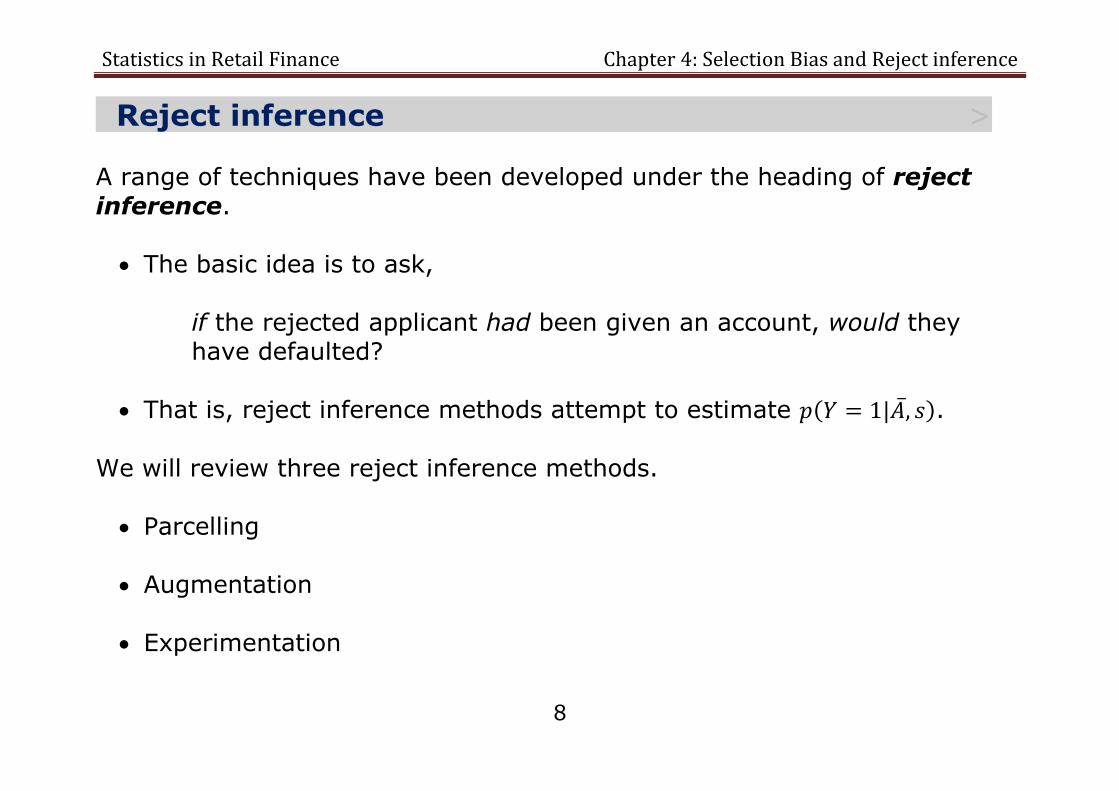
Reject inference > A range of techniques have been developed under the heading of reject

inference.

The basic idea is to ask,

if the rejected applicant had been given an account, would they have defaulted?

That is, reject inference methods attempt to estimate ( ̅ ). We will review three reject inference methods.

Parcelling Augmentation

Experimentation


9

Reject inference: Parcelling >

Parcelling is an approach based on regression imputation of missing values,

regressing responses where they are missing, based on a regression model built on the accepted applications.

It is a three-step approach which allows us to simulate values for the

missing outcomes for rejected applications (YR).

1. Build a model on just the accepted applicants as usual to get the

scorecard A. 2. Simulate outcomes for rejected applications based on values given by

scorecard A.

3. Build a new model with accepted applicants and simulated outcomes for rejects to get scorecard P.


10

Parcelling illustration >

XS

Observations

Selected

Model P

Actual Outcomes

YS

XR

Model A

(biased) Simulated Outcomes


11

Parcelling: How to simulate outcomes >

There are several ways to simulate outcomes.

Typically, two approaches are used.

1. Simulate a 0/1 outcome for each rejected applicant :- For each reject, generate a uniformly distributed random number

[ ]. Then a reject with score , computed with scorecard A, is simulated

with if and only if ( ). 2. Simulate 0/1 outcomes with probabilities:-

Include each reject twice: o once with and weight ( ), and

o once with and weight ( ). Real outcomes (from accepted applicants) are given weight 1.

Note that the overall weight for each applicant is always 1, but for rejects this weight is shared between the possible good and bad outcomes.


12

Option 1 is more realistic, but has a random element. Repeated simulations would be needed to ensure a stable result.

Option 2 is more complicated but is deterministic.


13

Including weights on observations > What is meant by putting a weight on an observation?

It means that as part of the estimation process, an observation will have

a weight on the estimate, relative to other observations.

Example. Normally an observation will have a weight 1, but if it is given a weight of 2 then it will be treated as though it were two observations.


14

Weights are easily implemented in maximum likelihood estimation as given weight values on each observation.

Suppose there are independent observations with log-likelihood function

given by

( ) ∑ ( )

Include given weights on each observation by generalizing this log-

likelihood function to

( ) ∑ ( )

Most statistical packages allow the inclusion of weights

(including the glm function in R).


15

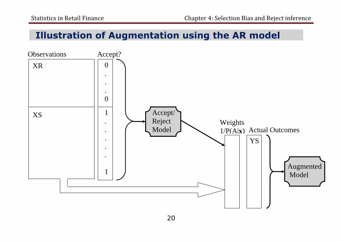
Reject inference: Augmentation > We assume there is some statistic Z, under which probability of outcome is

equalized between rejects and accepts:

( ̅ ) ( ) Typically, Z is taken as the score obtained by building an accept-reject (AR) model to differentiate rejects from accepts based on their borrower characteristics.

Notice that this will be a different scorecard to the one that is based

on, since this differentiates defaults and non-defaults.

The idea is that Z provides information about the rejects which allows the probabilities of outcome to be calibrated between rejects and accepts.


16

Augmentation using Accept/Reject model > A popular approach is to build a model which discriminates between accepts

and rejects, called an accept/reject (AR) model.

The score from the AR model is then used as the Z statistic.

The idea is that categories of observations that are under-represented within the accepted applicants are given greater weight in the estimation. This would mean that the distribution of rejects is better represented during

the estimation. If ( ) is the probability an application is accepted given it is in some

category , then it is reweighted by

( )

within the estimation.


17

Example 4.1.

Suppose a data set of 1000 applications has the following numbers within each employment category.

Employed Unemployed Self-employed

Retired Student Total

Rejects 100 (25%)

200 (50%)

40 (10%)

20 (5%)

40 (10%)

400

Accepted 330

(55%)

30

(5%)

60

(10%)

60

(10%)

120

(20%)

600

It is clear that amongst the accepts, the unemployed are under-

represented.


18

Therefore, get the probability of being accepted within each category and re-weight observations in each category accordingly.

Employed Unemployed Self-

employed

Retired Student

( )

=0.77 =0.13 =0.6 =0.75 =0.75 1.3 7.7 1.7 1.3 1.3

Therefore estimating with these weights will emphasize the unemployed observations within the accepted data set to compensate for their under-representation.


19

Using the Accept/Reject model > Example 4.1 illustrates the augmentation approach for a given age

category. But why age? How do we decide which category to use?

We do not have to! We can build an AR model and base probability of accept on that.

In particular an AR model will give us the probability ( ) which is all we

need. Then, ( ).

Note, the AR model can be built using logistic regression just like the scorecard model.


20

Illustration of Augmentation using the AR model >

XS

Observations

Weights

1/P(A|x)

Accept/

Reject

Model Actual Outcomes

XR

Augmented

Model

Accept?

0

.

.

.

0

1

.

.

.

.

.

1

YS


21

Example of augmentation > Do these methods of parcelling and augmentation actually work? There is

some debate about this. One problem is that in the real world, they are not testable!

However, simulation studies show that in some circumstances (but not all!)

they can be effective. Example 4.2.

Simulate 25,000 applications with two predictor variables: income and

ndel = number of delinquencies on record from other loans; and, also, an outcome { } is also generated for each application:

1=default; 0=non-default.

Because we are simulating, we have YR (remember, in the real world, this is not available).


22

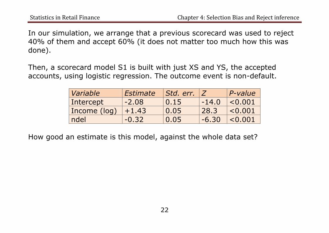
In our simulation, we arrange that a previous scorecard was used to reject 40% of them and accept 60% (it does not matter too much how this was

done). Then, a scorecard model S1 is built with just XS and YS, the accepted

accounts, using logistic regression. The outcome event is non-default.

Variable Estimate Std. err. Z P-value

Intercept -2.08 0.15 -14.0 <0.001

Income (log) +1.43 0.05 28.3 <0.001

ndel -0.32 0.05 -6.30 <0.001

How good an estimate is this model, against the whole data set?


23

Normally, in the real world, we could not answer this question. However, since this is a simulation, we have simulated outcomes for the rejects, YR,

and so can build an unbiassed model S2 using XR,YR and XS,YS. The result is:-


Intercept -2.05 0.046 -44.2 <0.001

Income (log) +1.47 0.018 80.9 <0.001

ndel -0.63 0.009 -74.1 <0.001

The results show that in S1, coefficient estimates on the intercept and Income (log) variable are good, but the estimate on the number of past

delinquencies (ndel) variable is poor. The estimate is almost half what we should expect without bias. Why is this happening?


24

This graph shows the distribution of ndel across all applicants and across accepts only.

It shows that those with high numbers of past delinquencies are under-represented.

Hence, the effect size of past delinquencies is underestimated

in model S1. This could have serious consequences, especially if past

delinquency is generally higher in future populations of applicants.

How could we improve the model without “cheating” (ie by looking at YR)?

0.0%

20.0%

40.0%

60.0%

80.0%

0 1 2 3 4 5

ndel

All applications Accepted applications


25

Try augmentation

When we augment, weights on accepted applications with higher values of ndel are generally higher. This has an effect on the coefficient estimates in the resulting model S3:-


Intercept -1.68 0.07 -22.8 <0.001

Income (log) +1.30 0.03 46.6 <0.001

ndel -0.38 0.03 -13.9 <0.001

This has now boosted the effect size of ndel (from -0.32), which is what we

want. But ultimately we are interested in predictions on an independent test set.

Can augmentation improve prediction results?


26

To test this, another 25,000 applications are simulated with outcome, following the same procedure. Test results using each model are given

below in AUC.

Model Description AUC

S1 Biassed model 0.832

S2 Benchmark unbiassed model 0.844

S3 Model with augmentation 0.840

These results show that the biassed model underperforms the unbiased model as we might expect.

The model with augmentation goes some way to improving on the biased model, but is not quite as good as the unbiased model.

But remember, in the real world, we could never build S2.

Only S1 and S3 are really possible.


27

Reject inference: Experimentation > The methods for parcelling, augmentation, and other similar methods, are

not ideal since they all make some assumptions about the rejects.

A statistically more rigorous approach is to run an experiment.

In the extreme case, a lender would not reject any applicants. o Then clearly, ( ) ( ). o Unfortunately, this would prove expensive and irresponsible since it

would result in many bad debts.

However, a lender can run a limited experiment by:

o Either allowing some applicants through with a slightly lower score

than the cut-off score; o Or, allowing a small proportion of those that would have been

categorized as rejects through as accepts.


28

This approach allows the lender to monitor cases of those that were categorized as rejects and therefore estimate ( ̅ ) on a small

sample, whilst controlling the cost of this experiment. Indeed, a costs analysis can be conducted to determine the optimal

proportion of “rejects” to allow through, in order to provide sufficient

and useful information to improve the scorecard calibration.

This approach has been used by mail order companies; retail banks that

are more conservative are less likely to use it.

There is a serious ethical issue with this practice, since lenders would be

deliberately providing loans to people they know are high risk. This would be viewed as highly irresponsible, even if it were done in a highly controlled way and may attract consumer complaints.


29

Reference > As mentioned in the notes, the selection bias problem for rejected

applications can be viewed as a special case of the missing value problem.

For background on the missing value problem, read

Little RJA and Rubin DB (1987), Statistical analysis with missing data, Wiley (available in the library)

The parcelling method is a form of regression imputation which is

described in this book.

Augmentation is related to the Weighting Method used in sample

surveys to deal with nonresponse. In this context, it is covered in Chapter 4 of the book.


30

Review of Chapter 4 >

We introduced the selection bias problem and considered three possible reject inference methods to try to solve the problem.

Parcelling Augmentation

Experimentation

statistics in retail finance chapter 4: selection bias and reject...

Documents