Statistics ITopic 4: Probability

Topic 4. Probability

Contents

I Random experiments, sample space, elementary and compositeevents.

I Definition of probability. Properties.

I Conditional probability and Multiplication Law. Independence.

I Law of Total Probability and Bayes’ Theorem.

Basic concepts: examples

I Random experiment: outcome of a die tossI Sample space (possible outcomes) finite: Ω = 1, 2, 3, 4, 5, 6I Elementary events (sample points): 1, 2, . . . , 6I Composite events: e.g., , A =“even outcome” = 2, 4, 6,

B =“outcome greater than 3”= 4, 5, 6.

I Random experiment: number of visits to UC3M’s web page nextMondayI Sample space countably infinite: Ω = 0, 1, 2, . . . = N ∪ 0I Elementary events: 0, 1, 2, . . .I Composite events: e.g., , A =“at least 100 visits” = 100, 101, . . .

and B =“less than 500 visits” = 0, 1, . . . , 499.

I Random experiment: closing price of a certain share of stock nextMondayI Sample space uncountably infinite: Ω = (0,+∞) or, Ω = (0,M) for

some M large enoughI Elementary events: x, with x ∈ ΩI Random events: e.g., A =“price larger than 5 euros” = (5,M) and

B =“price between 3 and 8 euros” = (3, 8).

Random events: basic conceptsEvents

I An event is a “reasonable” subset A of the sample space Ω (A ⊆ Ω).If the outcome ω of the random experiment satisfies that ω ∈ A, theevent happens. Otherwise, event A does not happen.

Trivial events

I Sure event: The complete sample space Ω. It always happens.

I Impossible event: The empty set ∅. It never happens.

Complementary event to an event A: event that happens when Adoes not happen. It comprises the elementary events of Ω that are not inA. We denote it by A or Ac .

Basic operations with random events

Suppose that A and B are events of the sample space Ω.

I Intersection of events: The intersection A ∩ B comprises all elementsthat are both in A and in B (A ∩ B: “A and B happen”).I A and B are incompatible events if they have no element in , i.e., if

their intersection is the impossible event, A ∩ B = ∅I Union of events: The union A ∪ B comprises all elements that are in

A or in B (A ∪ B: “A or B happen”).

I Difference of events: The difference A \ B comprises all elements ofA that are not in B (A \ B: “A happens but not B”).

De Morgan’s LawsRelations between the entre la union, intersection and complementaryevents:

A ∪ B = A ∩ B

A ∩ B = A ∪ B

Example: die tossing

Random experiment “tossing a die”:

I Sample space: Ω = 1, 2, 3, 4, 5, 6I Elementary events: 1, 2, 3, 4, 5, 6I Composite events: e.g., , A = 2, 4, 6, B = 4, 5, 6

Event A happens when “the outcome is even”.Event B happens when “the outcome is larger than 3”.

Example: die tossing

Ω = 1, 2, 3, 4, 5, 6 A = 2, 4, 6 B = 4, 5, 6

I Complementary:

A = 1, 3, 5 B = 1, 2, 3

I Intersection:

A ∩ B = 4, 6 A ∩ B = 1, 3

I Union:A ∪ B = 2, 4, 5, 6 A ∪ B = 1, 2, 3, 5

A ∪ A = 1, 2, 3, 4, 5, 6 = Ω

I Incompatible events:A ∩ A = ∅

Probability. Intuition

The probability of an event is a measure of the confidence we have apriori in that the event will happen when the random experiment takesplace (the larger the probability of an event, the higher the confidencethat it will happen).

When tossing a fair die: Intuitively,

I The probability that the outcome is 1 is less than the probabilitythat the outcome is larger than 1.

I The probability of getting a 4 is equal to that of getting a 6.

I The probability of getting a 7 is minimal, since it is an impossibleevent.

I The probability of getting a positive number is maximal, as it is asure event.

Three approaches/interpretations

Classical probability (Laplace’s Rule): It considers randomexperiments where all elementary events are equiprobable. If event A hasn(A) sample points, then we define the probability of A as

P(A) =number of cases favorable to A

number of possible cases=

n(A)

n(Ω).

Frequentist approach: If the experiment were to be repeated manytimes, the relative frequency of event A happening would converge to itsprobability.

P(A) = limiting frequency of event A

Subjetive probability: It depends on the available information.

P(A) = degree of belief or certainty that event A will happen

Probability: Axioms and properties

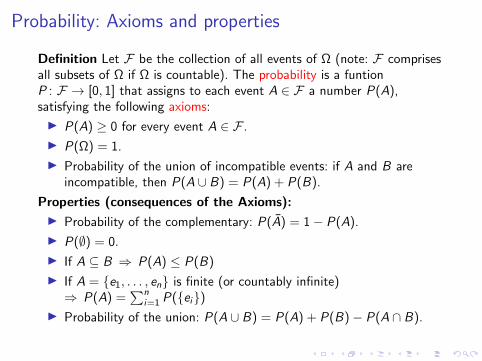
Definition Let F be the collection of all events of Ω (note: F comprisesall subsets of Ω if Ω is countable). The probability is a funtionP : F → [0, 1] that assigns to each event A ∈ F a number P(A),satisfying the following axioms:

I P(A) ≥ 0 for every event A ∈ F .

I P(Ω) = 1.

I Probability of the union of incompatible events: if A and B areincompatible, then P(A ∪ B) = P(A) + P(B).

Properties (consequences of the Axioms):

I Probability of the complementary: P(A) = 1− P(A).

I P(∅) = 0.

I If A ⊆ B ⇒ P(A) ≤ P(B)

I If A = e1, . . . , en is finite (or countably infinite)⇒ P(A) =

∑ni=1 P(ei)

I Probability of the union: P(A ∪ B) = P(A) + P(B)− P(A ∩ B).

Example: fair die tossing

I Probability of elementary events: P(i) = 16 , i = 1, . . . , 6

I Probability of even outcome: A = 2, 4, 6, hence

P(A) = P(2) + P(4) + P(6) =1

6+

1

6+

1

6=

1

2=

n(A)

n(Ω)

I Probability of outcome larger than 3: B = 4, 5, 6, hence

P(B) = P(4) + P(5) + P(6) =1

6+

1

6+

1

6=

1

2=

n(B)

n(Ω)

I Probability of odd outcome:

P(A) = 1− P(A) = 1− 1

2=

1

2

Example: fair die tossing

I Probability that outcome is even or greater than 3:

P(A ∪ B) = P(A) + P(B)− P(A ∩ B)

Since A ∩ B = 4, 6, P(A ∩ B) = 26 = 1

3 = n(A∩B)n(Ω) , y

P(A ∪ B) =1

2+

1

2− 1

3=

4

6=

2

3=

n(A ∪ B)

n(Ω)

I Probability that outcome is even or equal to 1.The events A = 2, 4, 6 and C = 1 are incompatible(A ∩ C = ∅), hence

P(A ∪ C ) = P(A) + P(C ) =1

2+

1

6=

4

6=

2

3=

n(A ∪ C )

n(Ω)

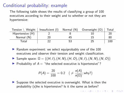
Conditional probability: exampleThe following table shows the results of classifying a group of 100executives according to their weight and to whether or not they arehypertensive:

Tension \ Weight Inssuficient (I) Normal (N) Overweight (O) Total

Hipertensive (H) 2 8 10 20Normal (N) 20 45 15 80

Total 22 53 25 100

I Random experiment: we select equiprobably one of the 100executives and observe their tension and weight classification.

I Sample space: Ω = (H, I ), (H,N), (H,O), (N, I ), (N,N), (N,O)I Probability of A = “the selected executive is hipertensive”?

P(A) =20

100= 0.2

(6= n(A)

n(Ω); why?

)I Suppose the selected executive is overweight. What is then the

probability (s)he is hipertensive? Is it the same as before?

Conditional probability: example

Probability of A (“is hipertensive”) given B (“is overweight”):

P(A |B)

To calculate it, we consider only the overweight executives:

P(A |B) =n(A ∩ B)

n(B)=

10

25= 0.4 > 0.2 = P(A)

The probability of an event depends on the available information

The conditional probability P(A |B) is the probability that A hap-pens given that we know B has happened.

Conditional probability. Independent events

Conditional probabilityDefinition: The probability of an event A given that another event B(with P(B) > 0) has happened is

P(A |B) =P(A ∩ B)

P(B)

Independent events

I Intuitively: knowing that one of the events has happened gives us noinformation about whether the other event has happened.

I Definition: Two events A and B are independent if

P(A ∩ B) = P(A)P(B).

I Property: Suppose that P(B) > 0. Then,A and B are independent ⇐⇒ P(A |B) = P(A)

Independent events: example

I Fair die toss

I Event A: outcome is even

I Event B: outcome is larger than 2

I We are told that B happened. Knowing this, what is the conditionalprobability that the outcome is even?

Independent events: example (cont.)

I Fair die toss

I Event A: outcome is even

I Event B: outcome is larger than 2

I We are told that B happened. Knowing this, what is the conditionalprobability that the outcome is even?

I

P(A |B) =P(A ∩ B)

P(B)=

2/6

4/6=

1

2= P(A).

I Events A and B are independent

Fundamental theorems of probability calculus

Multiplication ruleUseful to compute the probability that several events happensimultaneously when the conditional probabilities are easy to calculate.

I P(A ∩ B) = P(A)P(B |A), provided that P(A > 0).

I P(A ∩ B ∩ C ) = P(A)P(B |A)P(C |A ∩ B), provided thatP(A ∩ B) > 0.

I It generalizes to calculate the probability of the intersection of nevents A1, . . . ,An.

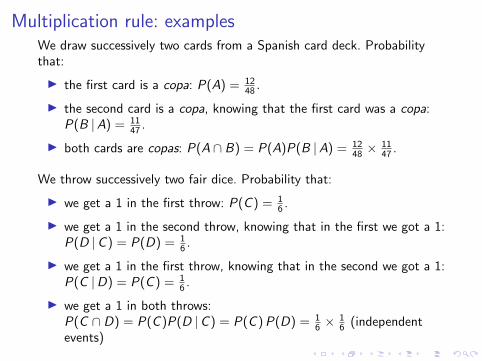
Multiplication rule: examplesWe draw successively two cards from a Spanish card deck. Probabilitythat:

I the first card is a copa: P(A) = 1248 .

I the second card is a copa, knowing that the first card was a copa:P(B |A) = 11

47 .

I both cards are copas: P(A ∩ B) = P(A)P(B |A) = 1248 ×

1147 .

We throw successively two fair dice. Probability that:

I we get a 1 in the first throw: P(C ) = 16 .

I we get a 1 in the second throw, knowing that in the first we got a 1:P(D |C ) = P(D) = 1

6 .

I we get a 1 in the first throw, knowing that in the second we got a 1:P(C |D) = P(C ) = 1

6 .

I we get a 1 in both throws:P(C ∩ D) = P(C )P(D |C ) = P(C )P(D) = 1

6 ×16 (independent

events)

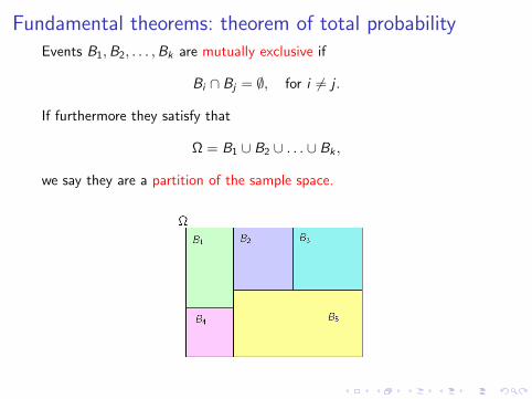
Fundamental theorems: theorem of total probabilityEvents B1,B2, . . . ,Bk are mutually exclusive if

Bi ∩ Bj = ∅, for i 6= j .

If furthermore they satisfy that

Ω = B1 ∪ B2 ∪ . . . ∪ Bk ,

we say they are a partition of the sample space.

Fundamental theorems: theorem of total probability

If B1,B2, . . . ,Bk is a partition of the sample space such that P(Bi ) 6= 0,i = 1, . . . , k , and A is any event, then

P(A) = P(A ∩ B1) + P(A ∩ B2) + . . . + P(A ∩ Bk) =

= P(A|B1)P(B1) + P(A|B2)P(B2) + . . . + P(A|Bk)P(Bk).

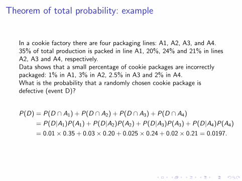
Theorem of total probability: example

In a cookie factory there are four packaging lines: A1, A2, A3, and A4.35% of total production is packed in line A1, 20%, 24% and 21% in linesA2, A3 and A4, respectively.Data shows that a small percentage of cookie packages are incorrectlypackaged: 1% in A1, 3% in A2, 2.5% in A3 and 2% in A4.What is the probability that a randomly chosen cookie package isdefective (event D)?

P(D) = P(D ∩ A1) + P(D ∩ A2) + P(D ∩ A3) + P(D ∩ A4)

= P(D|A1)P(A1) + P(D|A2)P(A2) + P(D|A3)P(A3) + P(D|A4)P(A4)

= 0.01× 0.35 + 0.03× 0.20 + 0.025× 0.24 + 0.02× 0.21 = 0.0197.

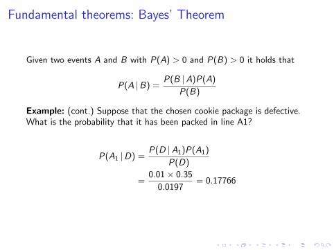
Fundamental theorems: Bayes’ Theorem

Given two events A and B with P(A) > 0 and P(B) > 0 it holds that

P(A |B) =P(B |A)P(A)

P(B)

Example: (cont.) Suppose that the chosen cookie package is defective.What is the probability that it has been packed in line A1?

P(A1 |D) =P(D |A1)P(A1)

P(D)

=0.01× 0.35

0.0197= 0.17766

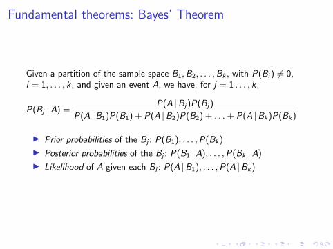
Fundamental theorems: Bayes’ Theorem

Given a partition of the sample space B1,B2, . . . ,Bk , with P(Bi ) 6= 0,i = 1, . . . , k , and given an event A, we have, for j = 1 . . . , k,

P(Bj |A) =P(A |Bj)P(Bj)

P(A |B1)P(B1) + P(A |B2)P(B2) + . . . + P(A |Bk)P(Bk)

I Prior probabilities of the Bj : P(B1), . . . ,P(Bk)

I Posterior probabilities of the Bj : P(B1 |A), . . . ,P(Bk |A)

I Likelihood of A given each Bj : P(A |B1), . . . ,P(A |Bk)

Bayes’ Theorem: example

• There is a clinical test for a rare disease affecting 1 of 10000 people

• The test gives a positive outcome (it detects the disease) in 99 out of100 people having it, and gives a negative outcome (it does not detect it)in 97 out of 100 people who do not have it.

• The test is applied to a randomly chosen person, and the outcome ispositive. What is the probability that the person has the disease?

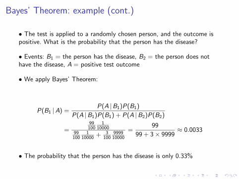
Bayes’ Theorem: example (cont.)

• The test is applied to a randomly chosen person, and the outcome ispositive. What is the probability that the person has the disease?

• Events: B1 = the person has the disease, B2 = the person does nothave the disease, A = positive test outcome

• We apply Bayes’ Theorem:

P(B1 |A) =P(A |B1)P(B1)

P(A |B1)P(B1) + P(A |B2)P(B2)

=99

1001

1000099

1001

10000 + 3100

999910000

=99

99 + 3× 9999≈ 0.0033

• The probability that the person has the disease is only 0.33%

Fundamental theorems: Applications

The theorem of total probability and Bayes’ theorem are especially usefulwhen:

I The random experiment can be organized in 2 stages

I It is easy to partition the sample space Ω through events B1, . . . ,Bk

corresponding to the first stage

I We know, or can easily calculate, the a priori probabilitiesP(B1), . . . ,P(Bk).

I We know, or can easily calculate, the likelihoodsP(A |B1), . . . ,P(A |Bk), where A is an event corresponding to thesecond stage .