statistics and modelling course 2011. topic 5: probability distributions achievement standard 90646...
TRANSCRIPT

Statistics and Modelling Course
2011

Topic 5: Probability Distributions
Achievement Standard 90646
Solve Probability Distribution Models to solve straightforward
problems
4 CreditsExternally Assessed
NuLake Pages 278 322

Binomial Distribution revision question:
NCEA 2009: Tom and Tane are surfers. Tom successfully rides a wave on average7 out of every 10 attempts, and Tane 6 out of every 10.Calculate the probability that Tom & Tane each ride 2 of the next 5waves.What assumptions must be made to use the Binomial Distn here?

Lesson 1: Intro to the Poisson Distribution.
Learning outcomes: Learn about what the Poisson Distribution is and its
parameter, . Learn the 4 requirements for the use of the Poisson
Distribution. Calculate probabilities using the Poisson Distribution.
1. Warm-up: 2009 NCEA q. on the Binomial Distn.2. The Poisson Distribution: Notes & examples using
the formula & tables (most of lesson).
HW: Sigma - Old edition: Ex. 6.1 or New: Ex. 16.01

The Poisson Distribution
Deals with rate of occurrence in an interval.
We use the Poisson Distribution when counting the number of occurrences of a discrete event over a given continuous interval (time/space).
Number of earthquakes per year (excluding after-shocks). Population density - Number of people per square km. House burglaries reported per week in Christchurch.

The Poisson Distribution
Deals with rate of occurrence in an interval.
We use the Poisson Distribution when counting the number of occurrences of a discrete event over a given continuous interval (time/space).
Number of earthquakes per year. Population density - Number of people per square km. House burglaries reported per week in Christchurch.
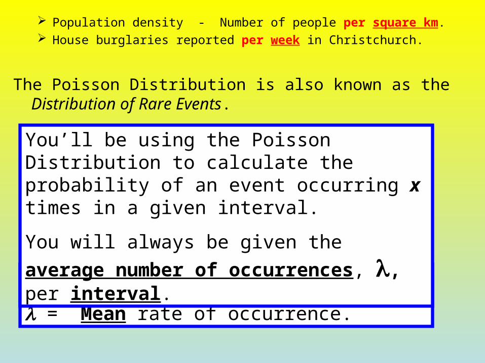
The Poisson Distribution is also known as the Distribution of Rare Events.

We use the Poisson Distribution when counting the number of occurrences of a discrete event over a given continuous interval (time/space).
Number of earthquakes per year. Population density - Number of people per square km. House burglaries reported per week in Christchurch.
The Poisson Distribution is also known as the Distribution of Rare Events.
You’ll be using the Poisson Distribution to calculate the probability of an event occurring x times in a given interval.
You will always be given the average
number of occurrences, , per interval. is the Greek symbol “Lambda”
Population density - Number of people per square km. House burglaries reported per week in Christchurch.
The Poisson Distribution is also known as the Distribution of Rare Events.
is the Greek symbol “Lambda”
= Mean rate of occurrence.
You’ll be using the Poisson Distribution to calculate the probability of an event occurring x times in a given interval.
You will always be given the average
number of occurrences, , per interval.
The Poisson Distribution is also known as the Distribution of Rare Events.
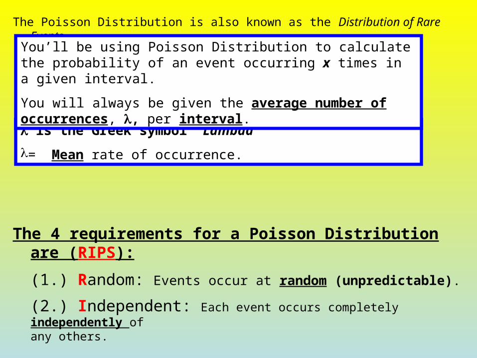
The 4 requirements for a Poisson Distribution are (RIPS):
(1.) Random: Events occur at random (unpredictable).
(2.) Independent: Each event occurs completely independently ofany others.
is the Greek symbol “Lambda”
= Mean rate of occurrence.
You’ll be using Poisson Distribution to calculate the probability of an event occurring x times in a given interval.
You will always be given the average number of occurrences, , per interval.

The 4 requirements for a Poisson Distribution are (RIPS):
(1.) Random: Events occur at random (unpredictable).
(2.) Independent: Each event occurs completely independently of any others.
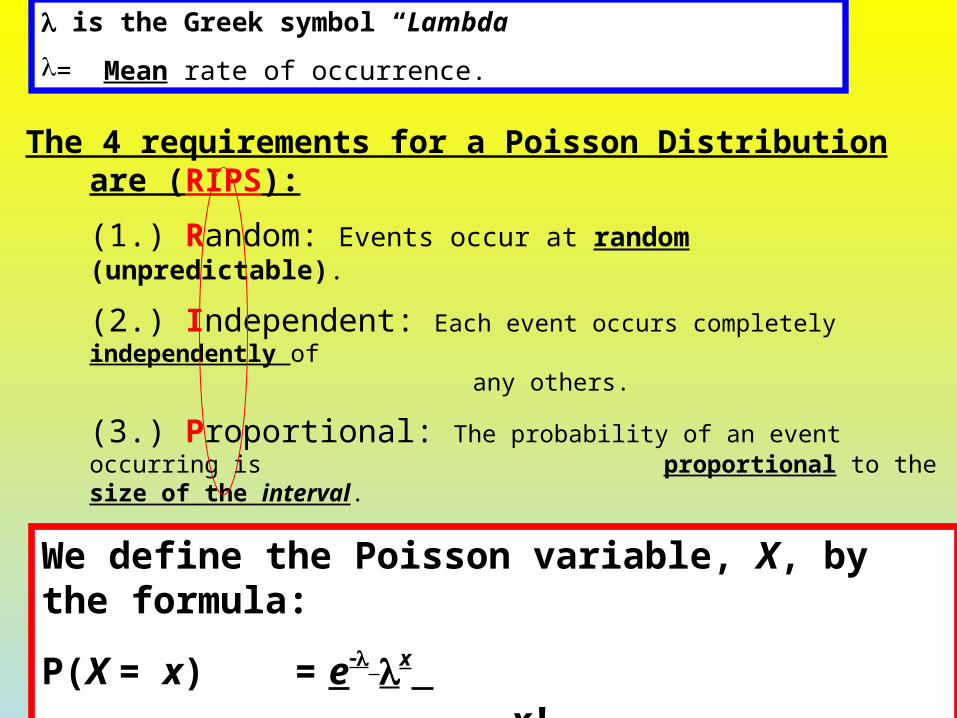
(3.) Proportional: The probability of an event occurring is proportional to the size of the interval.
(4.) Simultaneous: Events CANNOT occur simultaneously (at the same time or in exactly the same spot).
is the Greek symbol “Lambda”
= Mean rate of occurrence.
You’ll be using the Poisson Distribution to calculate the probability of an event occurring x times in a given interval.
You will always be given the average number of occurrences, , per interval.
The 4 requirements for a Poisson Distribution are (RIPS):
(1.) Random: Events occur at random (unpredictable).
(2.) Independent: Each event occurs completely independently ofany others.
(3.) Proportional: The probability of an event occurring isproportional to the size of the interval.
(4.) Simultaneous: Events CANNOT occur simultaneously (at the same time or in exactly the same spot).
is the Greek symbol “Lambda”
= Mean rate of occurrence.
We define the Poisson variable, X, by the formula:
P(X = x) = ex x!

(1.) Random: Events occur at random (unpredictable).
(2.) Independent: Each event occurs completely independently ofany others.
(3.) Proportional: The probability of an event occurring isproportional to the size of the interval.
(4.) Simultaneous: Events cannot occur simultaneously (at the same time or in exactly the same spot).
We define the Poisson variable, X, by the formula:
P(X = x) = ex x!
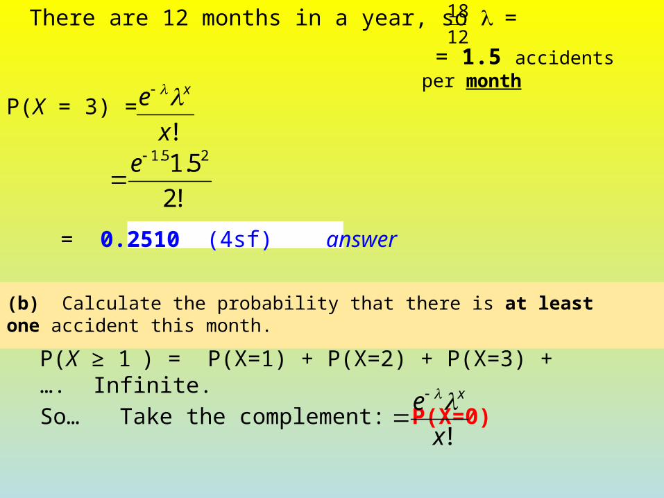
Eg: The average number of accidents at a particular intersection everyyear is 18.(a) Calculate the probability that there are exactly 2 accidents there this month.

Eg: The average number of accidents at a particular intersection everyyear is 18.(a) Calculate the probability that there are exactly 2 accidents there this month.
P(X = 2) =
?
(b) Calculate the probability that there is at least one accident this month.
12
18
= 1.5 accidents per month
!x
e x
!2
5.1 25.1
e
= 0.2510 (4sf) answer
There are 12 months in a year, so =

P(X = 3) =
(b) Calculate the probability that there is at least one accident this month.
12
18
= 1.5 accidents per month
!x
e x
!2
5.1 25.1
e
= 0.2510 (4sf) answer
There are 12 months in a year, so =
P(X ≥ 1 ) = P(X=1) + P(X=2) + P(X=3) + …. Infinite.
So…
P(X = 3) =
(b) Calculate the probability that there is at least one accident this month.
12
18
= 1.5 accidents per month
!x
e x
!2
5.1 25.1
e
= 0.2510 (4sf) answer
There are 12 months in a year, so =
P(X ≥ 1 ) = P(X=1) + P(X=2) + P(X=3) + …. Infinite.
So… Take the complement: P(X=0)!x
e x

P(X = 3) =
(b) Calculate the probability that there is at least one accident this month.
!x
e x
!2
5.1 25.1
e
= 0.2510 (4sf) answer
P(X ≥ 1 ) = P(X=1) + P(X=2) + P(X=3) + …. Infinite.
So… Take the complement: P(X=0)!x
e x
!0
5.1 05.1
e

(b) Calculate the probability that there is at least one accident this month.
= 0.2510 (4sf) answer
P(X ≥ 1 ) = P(X=1) + P(X=2) + P(X=3) + …. Infinite.
So… Take the complement: P(X=0)!x
e x
!0
5.1 05.1
e
5.1e1
15.1
e
= 0.223130…

(b) Calculate the probability that there is at least one accident this month.
P(X ≥ 1 ) = P(X=1) + P(X=2) + P(X=3) + …. Infinite.
So… Take the complement: P(X=0)!x
e x
!0
5.1 05.1
e
5.1e
= 0.223130…
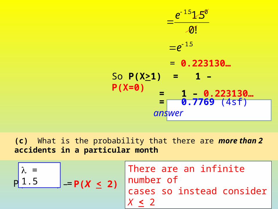
So P(X>1) = 1 – P(X=0) = 1 – 0.223130…
= 0.7769 (4sf) answer

P(X ≥ 1 ) = P(X=1) + P(X=2) + P(X=3) + …. Infinite.
So… Take the complement: P(X=0)!x
e x
!0
5.1 05.1
e
5.1e
= 0.223130…
So P(X>1) = 1 – P(X=0) = 1 – 0.223130…
= 0.7769 (4sf) answer
(c) What is the probability that there are more than 2 accidents in a particular month
!0
5.1 05.1
e
5.1e
= 0.223130…
So P(X>1) = 1 – P(X=0) = 1 – 0.223130…
= 0.7769 (4sf) answer
(c) What is the probability that there are more than 2 accidents in a particular month
P(X > 2 ) =
There are an infinite number of cases so instead consider X < 2
1 – P(X < 2)
= 1.5

So P(X>1) = 1 – P(X=0) = 1 – 0.223130…
= 0.7769 (4sf) answer
(c) What is the probability that there are more than 2 accidents in a particular month
P(X > 2 ) =
There are an infinite number of cases so instead consider X < 2
1 – P(X < 2)
= 1.5
= 1 – [ P(X =0) + P(X=1) + P(X=2)] Look up Poisson Tables
= 1 – [ _____ + ______ + ______]

= 1 – [ P(X =0) + P(X=1) + P(X=2)]
b P(X > 2 ) =
There are an infinite number of cases so instead consider X < 2
1 – P(X < 2)
= 1.5
Look up Poisson Tables
= 1 – [ _____ + ______ + ______]
c What is the probability that there are more than 2 accidents in a particular month
= 1 – 0.223130…
= 0.7769 (4sf) answer

If = 1.5,P(X = 0) = ?

If = 1.5,P(X = 0) = 0.2231

= 1 – [ P(X =0) + P(X=1) + P(X=2)]
b P(X > 2 ) =
There are an infinite number of cases so instead consider X < 2
1 – P(X < 2)
= 1.5
Look up Poisson Tables
= 1 – [ _____ + ______ + ______]
c What is the probability that there are more than 2 accidents in a particular month
= 1 – 0.223130…
= 0.7769 (4sf) answer

b P(X > 2 ) =
There are an infinite number of cases so instead consider X < 2
1 – P(X < 2)
= 1.5
Look up Poisson Tables
= 1 – [ 0.2231 + ______ + ______]
c What is the probability that there are more than 2 accidents in a particular month
= 1 – [ P(X =0) + P(X=1) + P(X=2)]
= 1 – 0.223130…
= 0.7769 (4sf) answer

If = 1.5,P(X = 0) = 0.2231

If = 1.5, P(X = 0) = 0.2231+ P(X = 1) = ?

If = 1.5, P(X = 0) = 0.2231+ P(X = 1) = 0.3347

= 1 – [ P(X =0) + P(X=1) + P(X=2)]
b P(X > 2 ) =
There are an infinite number of cases so instead consider X < 2
1 – P(X < 2)
= 1.5
Look up Poisson Tables
= 1 – [ 0.2231 + ______ + ______]
c What is the probability that there are more than 2 accidents in a particular month
= 1 – 0.223130…
= 0.7769 (4sf) answer

b P(X > 2 ) =
There are an infinite number of cases so instead consider X < 2
1 – P(X < 2)
= 1.5
Look up Poisson Tables
= 1 – [ 0.2231 + 0.3347 + ______]
c What is the probability that there are more than 2 accidents in a particular month
= 1 – [ P(X =0) + P(X=1) + P(X=2)]
= 1 – 0.223130…
= 0.7769 (4sf) answer

If = 1.5, P(X = 0) = 0.2231+ P(X = 1) = 0.3347

If = 1.5, P(X = 0) = 0.2231+ P(X = 1) = 0.3347+ P(X = 2) = ?

If = 1.5, P(X = 0) = 0.2231+ P(X = 1) = 0.3347+ P(X = 2) = 0.2510

b P(X > 2 ) =
There are an infinite number of cases so instead consider X < 2
1 – P(X < 2)
= 1.5
Look up Poisson Tables
= 1 – [ 0.2231 + 0.3347 + ______]
c What is the probability that there are more than 2 accidents in a particular month
= 1 – [ P(X =0) + P(X=1) + P(X=2)]
= 1 – 0.223130…
= 0.7769 (4sf) answer

b P(X > 2 ) =
There are an infinite number of cases so instead consider X < 2
1 – P(X < 2)
= 1.5
Look up Poisson Tables
= 1 – [ 0.2231 + 0.3347 + 0.2510]
c What is the probability that there are more than 2 accidents in a particular month
= 1 – [ P(X =0) + P(X=1) + P(X=2)]
= 1 – 0.223130…
= 0.7769 (4sf) answer

If = 1.5, P(X = 0) = 0.2231+ P(X = 1) = 0.3347+ P(X = 2) = 0.2510 P(X<2) =

If = 1.5, P(X = 0) = 0.2231+ P(X = 1) = 0.3347+ P(X = 2) = 0.2510 P(X<2) = 0.8088

b P(X > 2 ) =
There are an infinite number of cases so instead consider X < 2
1 – P(X < 2)
= 0.1912
HW: Sigma:Old edition: Ex. 6.1 or
New edition: Ex. 16.01
= 1.5
Look up Poisson Tables
= 1 – [ 0.2231 + 0.3347 + 0.2510]
c What is the probability that there are more than 2 accidents in a particular month
= 1 – [ P(X =0) + P(X=1) + P(X=2)]
= 1 – 0.8088
= 1 – 0.223130…
= 0.7769 (4sf) answer

Lesson 2: Poisson probabilities using a Graphics calculator
Learning outcome:Practice calculating probabilities of
combined events using the Poisson Distribution, using both tables and GC.
Work:1.HW qs.2.Problem on board – how to use your GC.3.Do Sigma (old – 2nd ed): p84 – Ex. 6.2 or in new version: p340 – Ex. 16.02

Poisson probabilities:Tables vs Graphics Calculator
E.g. Calculate P (X>3) for =4
USING TABLES. Do not copy this.
P(X>3) = 1 – P(X<3)
= 1 – [P(X=0) + P(X=1) + P(X=2) + P(X=3)]

Poisson probabilities:Tables vs Graphics Calculator
E.g. Calculate P (X>3) for =4
USING TABLES. Do not copy this.
P(X>3) = 1 – P(X<3)
= 1 – [P(X=0) + P(X=1) + P(X=2) + P(X=3)]
= 1 – [0.018315 + 0.073262 + 0.14652 + 0.19536]

Poisson probabilities:Tables vs Graphics Calculator
E.g. Calculate P (X>3) for =4
USING TABLES. Do not copy this.
P(X>3) = 1 – P(X<3)
= 1 – [P(X=0) + P(X=1) + P(X=2) + P(X=3)]
= 1 – [0.018315 + 0.073262 + 0.14652 + 0.19536]
= 1 – 0.433457
= 0.5665(4sf)

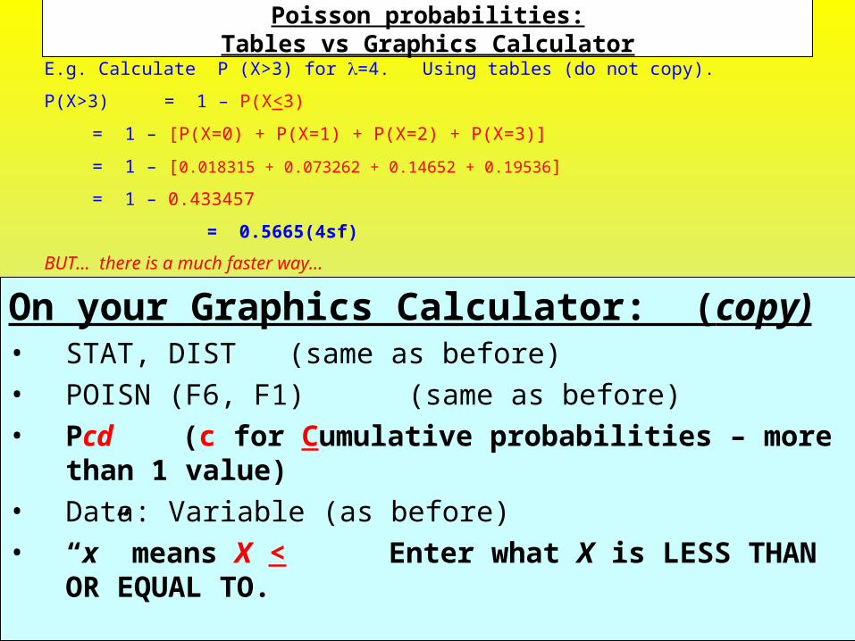
Poisson probabilities:Tables vs Graphics Calculator
E.g. Calculate P (X>3) for =4. Using tables (do not copy).
P(X>3) = 1 – P(X<3)
= 1 – [P(X=0) + P(X=1) + P(X=2) + P(X=3)]
= 1 – [0.018315 + 0.073262 + 0.14652 + 0.19536]
= 1 – 0.433457
= 0.5665(4sf)
BUT… there is a much faster way…
On your Graphics Calculator: (copy)

Poisson probabilities:Tables vs Graphics Calculator
E.g. Calculate P (X>3) for =4. Using tables (do not copy).
P(X>3) = 1 – P(X<3)
= 1 – [P(X=0) + P(X=1) + P(X=2) + P(X=3)]
= 1 – [0.018315 + 0.073262 + 0.14652 + 0.19536]
= 1 – 0.433457
= 0.5665(4sf)
BUT… there is a much faster way…
On your Graphics Calculator: (copy)• STAT, DIST (same as before)

Poisson probabilities:Tables vs Graphics Calculator
E.g. Calculate P (X>3) for =4. Using tables (do not copy).
P(X>3) = 1 – P(X<3)
= 1 – [P(X=0) + P(X=1) + P(X=2) + P(X=3)]
= 1 – [0.018315 + 0.073262 + 0.14652 + 0.19536]
= 1 – 0.433457
= 0.5665(4sf)
BUT… there is a much faster way…
On your Graphics Calculator: (copy)• STAT, DIST (same as before)• POISN (F6, F1) (same as before)

Poisson probabilities:Tables vs Graphics Calculator
E.g. Calculate P (X>3) for =4. Using tables (do not copy).
P(X>3) = 1 – P(X<3)
= 1 – [P(X=0) + P(X=1) + P(X=2) + P(X=3)]
= 1 – [0.018315 + 0.073262 + 0.14652 + 0.19536]
= 1 – 0.433457
= 0.5665(4sf)
BUT… there is a much faster way…
On your Graphics Calculator: (copy)• STAT, DIST (same as before)• POISN (F6, F1) (same as before)• Pcd (c for Cumulative probabilities – more than 1 value)

Poisson probabilities:Tables vs Graphics Calculator
E.g. Calculate P (X>3) for =4. Using tables (do not copy).
P(X>3) = 1 – P(X<3)
= 1 – [P(X=0) + P(X=1) + P(X=2) + P(X=3)]
= 1 – [0.018315 + 0.073262 + 0.14652 + 0.19536]
= 1 – 0.433457
= 0.5665(4sf)
BUT… there is a much faster way…
On your Graphics Calculator: (copy)• STAT, DIST (same as before)• POISN (F6, F1) (same as before)• Pcd (c for Cumulative probabilities – more than 1 value)• Data: Variable (as before)
Poisson probabilities:Tables vs Graphics Calculator
E.g. Calculate P (X>3) for =4. Using tables (do not copy).
P(X>3) = 1 – P(X<3)
= 1 – [P(X=0) + P(X=1) + P(X=2) + P(X=3)]
= 1 – [0.018315 + 0.073262 + 0.14652 + 0.19536]
= 1 – 0.433457
= 0.5665(4sf)
BUT… there is a much faster way…
On your Graphics Calculator: (copy)• STAT, DIST (same as before)• POISN (F6, F1) (same as before)• Pcd (c for Cumulative probabilities – more than 1 value)• Data: Variable (as before)• “x” means X < Enter what X is LESS THAN OR EQUAL
TO.
Note: Ppd gives individual Poisson probabilities, eg P(X=2), Pcd gives cumulative Poisson probabilities, eg P(X ≤ 2)

Poisson probabilities: Tables vs Graphics Calculator
Setting out of working when using your Graphics Calculator:
E.g. Calculate P (X > 3) for =4
P(X > 3) = 1 – P(X < 3)
= 1 – 0.433457 (G.C.)
= 0.5665(4sf)
On your Graphics Calculator: (copy)• STAT, DIST (same as before)• POISN (F6, F1) (same as before)• Pcd (c for Cumulative probabilities – more than 1 value)• Data: Variable (as before)• “x” means X < Enter what X is LESS THAN OR EQUAL
TO.
Note: Ppd gives individual Poisson probabilities, eg P(X=2), Pcd gives cumulative Poisson probabilities, eg P(X ≤ 2)

16.02BThe mean number of volcanic eruptions on White Island is 1.2 per year. Calculate the probability that there are more than 2 in one year.
P(X > 2) = 1– P(X ≤ 2)As this is infinite, rewrite > in terms of ≤
= 1– 0.879 48 (G.C.)
= 0.1205 (4sf)
=
Do old Sigma p84: Ex. 6.2
In new version: p340 – Ex. 16.02

Lesson 3: Inverse Poisson problems.
Learning outcomes:Calculate the variance & standard deviation
of a Poisson probability distribution.Solve inverse Poisson problems.
STARTER: Look at a graph of the Poisson Distribution (see Sigma workbook CD)
1.Variance & SD of Poisson – notes & e.gs Sigma 2nd ed: p89 – Ex. 6.3; New Sigma: p344 – Ex. 16.03
2. Inverse Poisson problems – notes & e.gs Sigma 2nd ed: p90 – Ex. 6.4; New Sigma: p347 – Ex. 16.04

Value of : 4.3 Investigate what happens for different values of between 0 and 30
x P(X = x ) Input these into cell B10 0.013571 0.05834 Questions2 0.12544 1 Describe a feature of the graph that is only apparent when is a counting number3 0.1798 2 Explain why the graph is always skewed to the right4 0.19328 3 What happens to the shape of the graph as the value of increases?
5 0.166226 0.119137 0.073188 0.039339 0.01879
10 0.0080811 0.0031612 0.0011313 0.0003714 0.0001115 3.3E-0516 8.9E-0617 2.2E-0618 5.4E-0719 1.2E-0720 2.6E-0821 5.3E-0922 1E-0923 1.9E-1024 3.5E-1125 6E-1226 9.9E-1327 1.6E-1328 029 030 031 032 0
0
0.05
0.1
0.15
0.2
0.25
0 1 2 3 4 5 6 7 8 9 10 11 12 13 14 15 16 17 18 19 20 21 22 23 24 25 26 27 28 29 30 31 32 33 34 35 36 37 38 39 40
P(X
= x
)
x
Poisson Probability Distribution

E.g.: A Poisson distribution has mean = 4.6. What is the standard deviation?
Standard deviation =
4.6
2.145
Do old Sigma p89: Ex. 6.3 – Q3 & 4
In new version: p345 – Ex. 16.03 – Q4 & 5
Variance & Standard Deviation of a Poisson Distn
= mean and also =variance.
So standard deviation, =

How to solve Inverse Poisson Questions
E.g.1: For a Poisson distribution, P(X = 0) = 0.0123. Calculate .
00.01230!
e Write out the Poisson formula
for the information given.

E.g.1: For a Poisson distribution, P(X = 0) = 0.0123. Calculate .
00.01230!
e Write out the Poisson formula
for the information given. 0.0123e
To calculate , take logs of both sides.
Simplify, using 0 and 0! both equal 1.
( ) (0.0123)n e nl l
Eg2: In samples of material taken from a textile factory, 40% had atleast one fault. Estimate the mean number of faults per sample.
Simplify, using loge e = 1 (cancels out). - = ln(0.0123)
= 4.398 (4sf)

E.g.1: For a Poisson distribution, P(X = 0) = 0.0123. Calculate .
00.01230!
e Write out the Poisson formula
for the information given. 0.0123e
To calculate , take logs of both sides.
Simplify, using 0 and 0! both equal 1.
( ) (0.0123)n e nl l
Eg2: In samples of material taken from a textile factory, 40% had atleast one fault. Estimate the mean number of faults per sample.
First choose the random variable, X.
Simplify, using loge e = 1 (cancels out). - = ln(0.0123)
= 4.398 (4sf)

Eg2: In samples of material taken from a textile factory, 40% had atleast one fault. Estimate the mean number of faults per sample.
Let X be ‘the number of faults per sample’
X has a Poisson distribution.
Given P(X ≥ 1) = 0.4
P(X = 0) = 0.6
Simplify, using 0 and 0! both equal 1
00.60!
e
0.6e
First choose the random variable, X.
Write out the Poisson formula for the information given.
To calculate , take logs of both sides.
As ≥ is infinite (no upper limit), we considerthe complement, knowing P(X>1) = 1- P(X=0)
- = ln(0.0123)
= 4.398 (4sf)
Simplify, using loge e = 1 (cancels out).

Eg2: In samples of material taken from a textile factory, 40% had atleast one fault. Estimate the mean number of faults per sample.
Let X be ‘the number of faults per sample’
X has a Poisson distribution.
Given P(X ≥ 1) = 0.4
P(X = 0) = 0.6
00.60!
e
0.6e
To calculate , take logs of both sides.
Simplify, using loge e = 1 (cancels out).
( ) (0.6)n e nl l
As ≥ is infinite (no upper limit), we considerthe complement, knowing P(X>1) = 1- P(X=0)
= 0.5108 (4sf)
- = ln(0.6)
Do old Sigma p90: Ex. 6.4
In new version: p347 – Ex. 16.04
Complete for HW
Lesson 4: Problems that involve the use of more than 1 type of distribution
Learning outcome:Solve problems involving a mixture of all 3 types of
distribution.Key skill: identifying the appropriate distribution to
use.
1. STARTER: Go over HW qs from Inverse Poisson chapter in Sigma.
2. Revision worksheet for all 3 Probability Distribution.
3. Do Sigma (NEW): p384 – Ex. 18.03. Finish Q13 for HW.

Problems that require the use of more than one type of probability
distribution

Problems that require the use of more than one type of probability
distribution
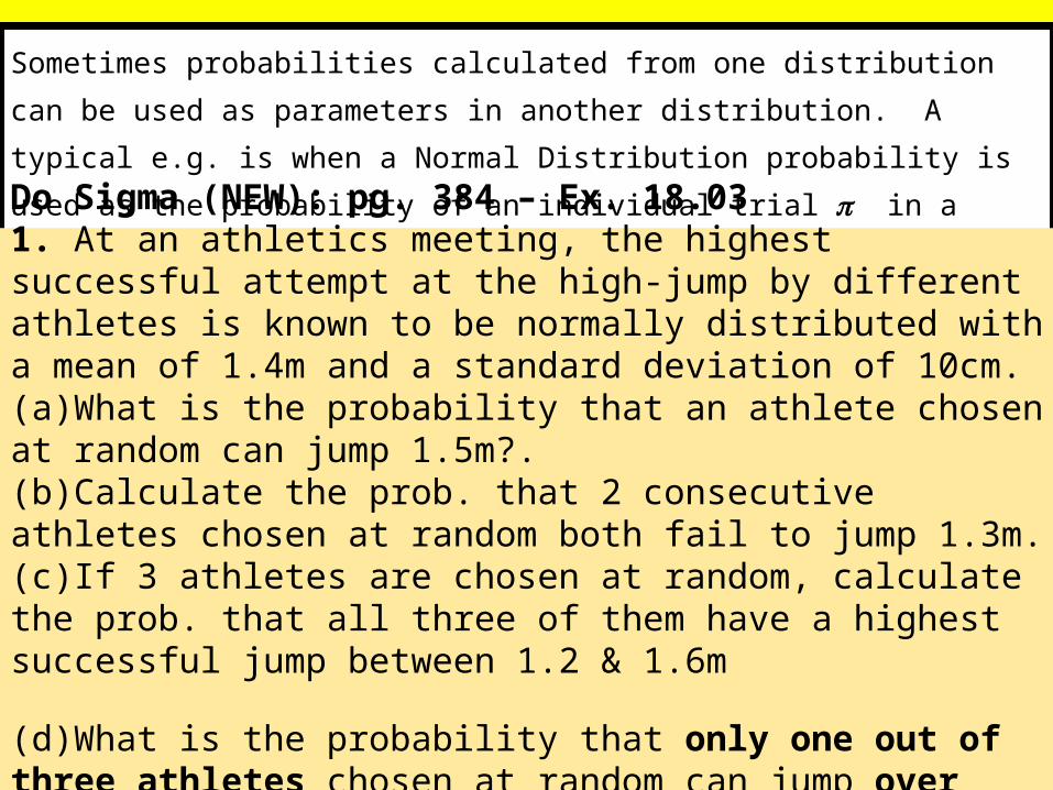
Sometimes probabilities calculated from one distribution can be used
as parameters in another distribution.

Problems that require the use of more than one type of probability
distribution
Sometimes probabilities calculated from one distribution can be used
as parameters in another distribution. A typical e.g. is when a Normal
Distribution probability is used as the probability of an individual trial
in a Binomial Distribution.
Do Sigma (NEW): pg. 384 – Ex. 18.03

Problems that require the use of more than one type of probability
distribution
Sometimes probabilities calculated from one distribution can be used
as parameters in another distribution. A typical e.g. is when a Normal
Distribution probability is used as the probability of an individual trial
in a Binomial Distribution.
Do Sigma (NEW): pg. 384 – Ex. 18.031. At an athletics meeting, the highest successful attempt at the high-jump by different athletes is known to be normally distributed with a mean of 1.4m and a standard deviation of 10cm.(a)What is the probability that an athlete chosen at random can jump 1.5m?.(b)Calculate the prob. that 2 consecutive athletes chosen at random both fail to jump 1.3m.(c)If 3 athletes are chosen at random, calculate the prob. that all three of them have a highest successful jump between 1.2 & 1.6m
(d)What is the probability that only one out of three athletes chosen at random can jump over 1.6m?

EXTENSION SESSION: Approximations – approximating
between all 3 distributions.Learning outcome:Solve problems involving a mixture of all 3 types of distribution.Key skill: identifying the appropriate distribution to use.
1. Handout on approximations (flow-chart). View applet (graphical demonstration using bar graphs)
2. Problems to get the hang of approximating – all in Sigma old edition:
Approximating between: - the Binomial with the Poisson: p121 – Ex. 8.2 Q1 & 2 only. - the Poisson with the Normal: p123– Ex. 8.3 Q1 & 2 only. - mixed approximation problems: p125 – Ex. 8.4. All.
HW: Challenge problem set.

APPROXIMATIONS
Only in scholarship exam now – see first version of NuLake (2004)
for concise notes.
Do chapter in Sigma 2nd edition.

Approximating from the Binomial Distribution to the Poisson
Can only use when: n is very large. is extreme (probabilities are very close to 0 or 1)
Question: Why must n be large and be close to 0 or 1?Hint: What do the Binomial and Poisson Dists have in common?Answer: Both model how often an event occurs (counting –
discrete).
Another hint:
n
Do “Comparing Models” handout, JUST THE FIRST PAGE. (from Achieving in Statistics workbook).

Approximating from the Binomial Distribution to the Poisson
Can only use when: n is very large. is extreme (probabilities are very close to 0 or 1)
Question: Why must n be large and be close to 0 or 1?Hint: What do the Binomial and Poisson Dists have in common?Answer: Both model how often an event occurs (counting – discrete).
Another hint: What is different about the Binomial & Poisson distributions?Answer: Binomial used when event occurs within a fixed number of trials
(discrete).Poisson used when event occurs within a continuous interval.
n

Approximations challenge problems
Problem 1:
In a certain suburb, 30% of new homes are built with an outdoor bbq area, and 2% of new homes require alterations after construction.
(a)A random sample of 50 homes is to be taken. Find the probability that no more than 20 homes in this sample will be built with an outdoor bbq area.
(b)Another sample of n new homes is to be taken. Find the value of n so that the probability that the sample contains no homes requiring alterations is approximately 0.6.

Approximations challenge problems
Problem 2:

TESTFormative assessment of
AS90646
Lesson 5:

Probability Distribution
Scholarship slides

The Normal Distribution
Scholarship slides

P( Z ) = 0.01
– 5 0
– 5 0
-2.33
STARTER: A product has a normally distributed weight with μ = 1kg. If the risk of marketing a product more than 50g underweight must be less than 1%, what is the maximum allowable standard deviation?
Solution:Let X be a random variable representing the weight of the product in grams.
We want such that P( X 950 ) = 0.01
P( Z ) = 0.01
For the maximum value of take P( Z ) = 0.01
950 – 1000
950 – 1000
– 5 0
– 5 0
And, we can use tables or graphics calcto find, based on prob of 0.01,z=-2.33…
Re-arranging to solve for …
33.250
z

P( Z ) = 0.01
-2.33
STARTER: A product has a normally distributed weight with μ = 1kg. If the risk of marketing a product more than 50g underweight must be less than 1%, what is the maximum allowable standard deviation?
Solution:Let X be a random variable representing the weight of the product in grams.
We want such that P( X 950 ) = 0.01
P( Z ) = 0.01
For the maximum value of take P( Z ) = 0.01
=
= 21.5
so 21.5 is the maximum allowable standard deviation
950 – 1000
950 – 1000
And, we can use tables or graphics calcto find, based on prob of 0.01,z=-2.33…
Re-arranging to solve for …
33.250
z

17.05A
Eg1: The weights of suitcases received by an airline at check-in can be modelled by a normal distribution with mean 17 kg and standard deviation 4 kg. The airline charges for excess baggage if a suitcase is ‘overweight’—defined as weighing more than 20 kg.a Find the probability that two consecutive passengers both have to pay for excess baggage.b What proportion of overweight suitcases weigh less than 22 kg?

Use your graphics calculator to work out the probability that a single suitcase is overweight to 4 sf.
Eg1: The weights of suitcases received by an airline at check-in can be modelled by a normal distribution with mean 17 kg and standard deviation 4 kg. The airline charges for excess baggage if a suitcase is ‘overweight’—defined as weighing more than 20 kg.a Find the probability that two consecutive passengers both have to pay for excess baggage.

P(excess)
= 0.2266
= P(X > 20)
Eg1: The weights of suitcases received by an airline at check-in can be modelled by a normal distribution with mean 17 kg and standard deviation 4 kg. The airline charges for excess baggage if a suitcase is ‘overweight’—defined as weighing more than 20 kg.a Find the probability that two consecutive passengers both have to pay for excess baggage.

Draw a tree diagram to show the possibilities for two suitcases.
P(X > 20) = 0.2266
Eg1: The weights of suitcases received by an airline at check-in can be modelled by a normal distribution with mean 17 kg and standard deviation 4 kg. The airline charges for excess baggage if a suitcase is ‘overweight’—defined as weighing more than 20 kg.a Find the probability that two consecutive passengers both have to pay for excess baggage.

Eg1: The weights of suitcases received by an airline at check-in can be modelled by a normal distribution with mean 17 kg and standard deviation 4 kg. The airline charges for excess baggage if a suitcase is ‘overweight’—defined as weighing more than 20 kg.a Find the probability that two consecutive passengers both have to pay for excess baggage.
P(two cases overweight)= 0.2266 0.2266
= 0.0513
P(X > 20) = 0.2266
Over weight
Under weight
Over weight
Under weight
Over weight
Under weight
0.2266
0.7734
0.2266
0.2266
0.7734
0.7734
*

Eg1: The weights of suitcases received by an airline at check-in can be modelled by a normal distribution with mean 17 kg and standard deviation 4 kg. The airline charges for excess baggage if a suitcase is ‘overweight’—defined as weighing more than 20 kg.b What proportion of overweight suitcases weigh less than 22 kg?
This is a conditional probability:
P(X < 22/X > 20) =
(20 22)( 20)
P XP X
0.120 977 50.226 627 3
= 0.5338 (4 sf)
that X < 22, given that X > 20
Do NuLake qs on “Combined Events for Poisson, Normal and Binomial”Q3134 (p303305 in 2007 edition)

a Draw a probability tree.
Eg2: Over a long period of time, the number of accidents per day on a certain road has been found to have a mean of 2 on weekdays and 3 at the weekend.a What is the probability that there are 3 accidents on a day chosen at random?b If there are no accidents on a particular day, calculate the probability that it is a weekday.

a
weekday
weekend
5/7
2/7
3 accidents
other than 3 accidents
3 accidents
other than 3 accidents
?
?
Calculate using Poisson = 2, x = 3
Eg2: Over a long period of time, the number of accidents per day on a certain road has been found to have a mean of 2 on weekdays and 3 at the weekend.a What is the probability that there are 3 accidents on a day chosen at random?b If there are no accidents on a particular day, calculate the probability that it is a weekday.

a
weekday
weekend
5/7
2/7
3 accidents
other than 3 accidents
3 accidents
other than 3 accidents
0.1804
?Calculate using Poisson = 3, x = 3
Eg2: Over a long period of time, the number of accidents per day on a certain road has been found to have a mean of 2 on weekdays and 3 at the weekend.a What is the probability that there are 3 accidents on a day chosen at random?b If there are no accidents on a particular day, calculate the probability that it is a weekday.

a
weekday
weekend
5/7
2/7
3 accidents
other than 3 accidents
3 accidents
other than 3 accidents
0.1804
0.2240
P(3 accidents) = 5/7 0.1804 + 2/7 0.2240
= 0.19 (2 dp)
Eg2: Over a long period of time, the number of accidents per day on a certain road has been found to have a mean of 2 on weekdays and 3 at the weekend.a What is the probability that there are 3 accidents on a day chosen at random?b If there are no accidents on a particular day, calculate the probability that it is a weekday.
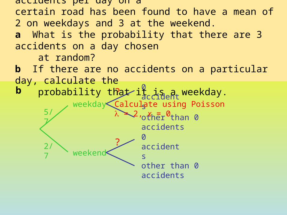
b
weekday
weekend
5/7
2/7
0 accidents
other than 0 accidents
0 accidents
other than 0 accidents
?
?
Calculate using Poisson = 2, x = 0
Eg2: Over a long period of time, the number of accidents per day on a certain road has been found to have a mean of 2 on weekdays and 3 at the weekend.a What is the probability that there are 3 accidents on a day chosen at random?b If there are no accidents on a particular day, calculate the probability that it is a weekday.

b
weekday
weekend
5/7
2/7
0 accidents
other than 0 accidents
0 accidents
other than 0 accidents
0.1353
?Calculate using Poisson = 3, x = 0
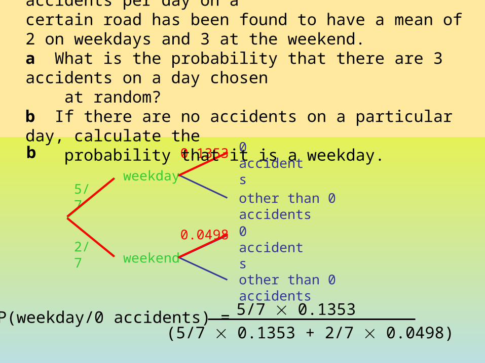
Eg2: Over a long period of time, the number of accidents per day on a certain road has been found to have a mean of 2 on weekdays and 3 at the weekend.a What is the probability that there are 3 accidents on a day chosen at random?b If there are no accidents on a particular day, calculate the probability that it is a weekday.

b
weekday
weekend
5/7
2/7
0 accidents
other than 0 accidents
0 accidents
other than 0 accidents
0.1353
0.0498
P(weekday/0 accidents) = P(weekday AND 0 accidents)
P( 0 accidents)
Eg2: Over a long period of time, the number of accidents per day on a certain road has been found to have a mean of 2 on weekdays and 3 at the weekend.a What is the probability that there are 3 accidents on a day chosen at random?b If there are no accidents on a particular day, calculate the probability that it is a weekday.

b
weekday
weekend
5/7
2/7
0 accidents
other than 0 accidents
0 accidents
other than 0 accidents
0.1353
0.0498
P(weekday/0 accidents) = 5/7 0.1353
P(0 accidents)
Eg2: Over a long period of time, the number of accidents per day on a certain road has been found to have a mean of 2 on weekdays and 3 at the weekend.a What is the probability that there are 3 accidents on a day chosen at random?b If there are no accidents on a particular day, calculate the probability that it is a weekday.
b
weekday
weekend
5/7
2/7
0 accidents
other than 0 accidents
0 accidents
other than 0 accidents
0.1353
0.0498
P(weekday/0 accidents) = 5/7 0.1353
(5/7 0.1353 + 2/7 0.0498)
Eg2: Over a long period of time, the number of accidents per day on a certain road has been found to have a mean of 2 on weekdays and 3 at the weekend.a What is the probability that there are 3 accidents on a day chosen at random?b If there are no accidents on a particular day, calculate the probability that it is a weekday.

b
weekday
weekend
5/7
2/7
0 accidents
other than 0 accidents
0 accidents
other than 0 accidents
0.1353
0.0498
P(weekday/0 accidents) = 0.0966
0.1109
Eg2: Over a long period of time, the number of accidents per day on a certain road has been found to have a mean of 2 on weekdays and 3 at the weekend.a What is the probability that there are 3 accidents on a day chosen at random?b If there are no accidents on a particular day, calculate the probability that it is a weekday.

b
weekday
weekend
5/7
2/7
0 accidents
other than 0 accidents
0 accidents
other than 0 accidents
0.1353
0.0498
P(weekday/0 accidents) = 0.8717 (4sf)
Eg2: Over a long period of time, the number of accidents per day on a certain road has been found to have a mean of 2 on weekdays and 3 at the weekend.a What is the probability that there are 3 accidents on a day chosen at random?b If there are no accidents on a particular day, calculate the probability that it is a weekday.

Eg3: A travel agent receives faxes from either within New Zealand or overseas. The probability that any given fax arrives from a New Zealand number is 0.75. One day the travel agent receives 10 faxes. If at least 6 are from New Zealand numbers, calculate the probability that only 1 of the 10 faxes is from overseas.
n = 10 and = 0.25
Suppose X = number of faxes from overseasState the random variable involved.Give the values of the two
parameters.What are we trying to find?
We want the probability that 1 fax is from overseas given that 4 or fewer are from overseas
( 1/ 4)P X X
( 1 4)( 4)
P X XP X
( 1)( 4)P XP X
= 0.18771 0.92187
= 0.2036 (4sf)
Using Graphics Calculator

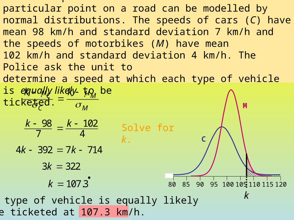
E.g.4: A traffic research unit has established that the speeds of both cars and motorbikes on a particular point on a road can be modelled by normal distributions. The speeds of cars (C) have mean 98 km/h and standard deviation 7 km/h and the speeds of motorbikes (M) have mean 102 km/h and standard deviation 4 km/h. The Police ask the unit to determine a speed at which each type of vehicle is equally likely to be ticketed.
80 85 90 95 100 105 110 115 120
C
M
The problem is to determine k such that P(C > k) = P(M > k).
The graph shows the relationship between the two distributions.

80 85 90 95 100 105 110 115 120
C
M
The problem is to determine k such that P(C > k) = P(M > k).
The required value has the same area to the right of it for each curve.
k
i.e. the two shaded areas must be the same.
E.g.4: A traffic research unit has established that the speeds of both cars and motorbikes on a particular point on a road can be modelled by normal distributions. The speeds of cars (C) have mean 98 km/h and standard deviation 7 km/h and the speeds of motorbikes (M) have mean 102 km/h and standard deviation 4 km/h. The Police ask the unit to determine a speed at which each type of vehicle is equally likely to be ticketed.

80 85 90 95 100 105 110 115 120
C
M
The problem is to determine k such that P(C > k) = P(M > k).
Note – this is not given by the point where the curves intersect!
The required value has the same area to the right of it for each curve.
k
E.g.4: A traffic research unit has established that the speeds of both cars and motorbikes on a particular point on a road can be modelled by normal distributions. The speeds of cars (C) have mean 98 km/h and standard deviation 7 km/h and the speeds of motorbikes (M) have mean 102 km/h and standard deviation 4 km/h. The Police ask the unit to determine a speed at which each type of vehicle is equally likely to be ticketed.

80 85 90 95 100 105 110 115 120
C
M
The problem is to determine k such that P(C > k) = P(M > k).
For the two probabilities to be equal, each curve must convert to the same z-value as the other
k
E.g.4: A traffic research unit has established that the speeds of both cars and motorbikes on a particular point on a road can be modelled by normal distributions. The speeds of cars (C) have mean 98 km/h and standard deviation 7 km/h and the speeds of motorbikes (M) have mean 102 km/h and standard deviation 4 km/h. The Police ask the unit to determine a speed at which each type of vehicle is equally likely to be ticketed.
80 85 90 95 100 105 110 115 120
C
M
k
C M
C M
k k
98 1027 4
k k
4 392 7 714k k
3 322k
Each type of vehicle is equally likely to be ticketed at 107.3 km/h.
Solve for k.
107.3k .
E.g.4: A traffic research unit has established that the speeds of both cars and motorbikes on a particular point on a road can be modelled by normal distributions. The speeds of cars (C) have mean 98 km/h and standard deviation 7 km/h and the speeds of motorbikes (M) have mean 102 km/h and standard deviation 4 km/h. The Police ask the unit to determine a speed at which each type of vehicle is equally likely to be ticketed.

The Binomial Distribution
Scholarship slides

Eg5 – University Stage 2 Probability exam q:In a particular game where I can either win or lose (assuming: a) theindependence among the outcomes of the games and; b) the sameprobability to win in each game); if the probability to win 3 games outof 3 is , what is the probability to win 2 out of 4?
27
1
Solution: Probability of winning a single game, is: 27
13
3
1
So prob. of winning 2 out of 4 games is found by the binomial distribution formula where n=4, x=2, and =1/3.
3
1,4,2 nxP
22
3
2
3
1
2
4
) (3sf .2960

The geometric distribution: probability that the 1st success occurs in the nth trial.
The negative binomial distribution: probability that the kth success occurs on the nth trial.