statistics and data analysis in geology (3rd_ed.)
TRANSCRIPT


Statistics and Data Analysis
Third Edition
John C. Davis Kansas Geological Survey The University of Kansas
John Wiley & Sons New York Clxchester Brisbane Toronto Singapore

ASSOCIATE EDITOR Mark Gerber MARKETING M A N A G E R Kevin Molloy PROGRAM COORDINATOR Denise Powell PRODUCTION EDITOR Brienna Berger DESIGNER Madelyn Lesure C O V E R PHOTO Bill B a c h m a d P h o t o Researchers
This book was printed and bound by Courier. The cover was printed by Phoenix Color.
Copyright tables and figures in this text are reproduced with permission of the copyright owners. The source for each table and figure is noted in its caption and a complete citation is given at the end of each chapter in Suggested Readings. Table A S is used with the permission of McGraw-Hill Companies. Tables A.6 and A.8 are copyright by John Wiley & Sons, Inc. and reproduced with permission. Parts of Table A.9 are copyright by the American Statistical Association and by the American Institute of Biological Sciences-the combined table is reproduced with permission. Tables A.10 and A.11 are copyright by Academic Press Inc. (London) and are reproduced with permission. Figure 2-25 is copyright by Harcourt Brace Jovanovich, Inc. Figure 5-22 is copyright by the American Statistical Association. Both illustrations are reproduced with permission.
Copyright 0 2002 by John Wiley & Sons, Inc. All rights reserved
No part of this publication may be reproduced, stored in a retrieval system or transmitted in any form or by any means, electronic, mechanical, photocopying, recording, scanning or otherwise, except as permitted under Sections 107 or 108 of the 1976 United States Copyright Act, without either the prior written permission of the Publisher, or authorization through payment of the appropriate per-copy fee to the Copyright Clearance Center, 222 Rosewood Drive, Danvers, MA 01 923, (508)750-8400, fax (508)750-4470. Requests to the Publisher for permission should be addressed to the Permissions Department, John Wiley & Sons, Inc., 605 Third Avenue, New York, NY 10158-0012, (212) 850-6011, fax (212) 850-6008, E-Mail: [email protected]. To order books or for customer service please call l(800) 225-5945.
ISBN 0-47 1-1 7275-8
Library of Congress Cataloging in Publication Data: Davis, John C.
Statistics and data analysis in geology-3'd ed. Includes bibliographies and index. 1, Geology-Data processing. 2. Geology- Statistical methods. I . Title
QE48.8 .D3 8 2002 550'.72 85-12331
Printed in the United States of America
10 9 8 7 G 5 4 3 2 1

Preface My original motivation for writing this book, back in 1973, was very simple. Teach- ing the techniques of data analysis to engineers and natural scientists, both uni- versity students and industry practitioners, would be easier, I reasoned, if I had a suitable textbook. It was. By 1986 when I revised Statistics and Data Analysis in Geology for its second edition, technology had progressed to the point that personal computers were almost commonplace and every young geologist was expected to have at least some familiarity with computing and analysis of data. This was a time of transition when personal computers offered the freedom of access and ease of use missing in the centralized mainframe environment, but these PC’s lacked the power and speed necessary for many geological applications. In the interven- ing years since the appearance of the second edition, computing technology has evolved with almost unbelievable speed. I now have on my desktop a small crys- talline cube, a “supercomputer” capable of outperforming devices that existed a decade ago at only a few sites in the world.
Although computing tools have advanced rapidly, our skills as educators have not kept pace. Almost all undergraduate students in the natural sciences and engi- neering, including the Earth sciences, are required to take classes in mathematics, statistics, data analysis, and computing. Graduate students, as a matter of course, are expected to have proficiency in these areas. Unfortunately, Earth science stu- dents voice an almost universal complaint: material taught in such courses is not relevant to their studies. In part this criticism reflects a certain mental rigidity present in some young minds that refuse to make an effort to stretch their imagi- nations. But it also reflects, in part, the absence of anything quantitative in many geology courses.
It is not surprising when students protest, “Why should I study this dull and boring topic when the material is never used in my field?” In an attempt to con- tribute to the solution of this educational impasse, I’ve made a major change in this edition of my book. The text now includes numerous geological data sets that illustrate how specific computational procedures can be applied to problems in the Earth sciences. In addition, each chapter ends with a set of exercises of greater or lesser complexity that the student can address using methods discussed in the text. It should be noted that there is no “teacher’s manual” containing correct answers. Like most real-world situations, there may be more than one solution to a problem. An answer may depend upon how a question is framed. Acknowledging that no students, not even graduate assistants, like to do drudge work such as data entry, I’ve provided all of the data for examples and exercises as digital files on the World Wide Web. Thus, while there may be many excuses for failing to work an exercise, entering data incorrectly should not be one of them!
We have already noted that computing technology has changed enormously during the 28 years this book has been in print. Computers are no longer made that can read floppy disks and double-sided diskettes are being phased out by optical disks. We can be sure that computer technology will continue to evolve at a dizzying pace; to provide some degree of security from obsolescence, the data files are available on the World Wide Web at two sites, one maintained by John Wiley & Sons and the other by the Kansas Geological Survey. The WWW addresses are
http://www.wiley.com/college/davis and
http://www.kgs. ku.edu/Mathgeo/Books/Stat/index.html
V

In addition to the downloadable files from the 3rd edition of Statistics and Data Anal- ysis in Geology, you may also find additional data sets and exercises at this site as they are made available from time to time.
The basic arrangement of topics covered in the book is retained from earlier editions, progressing from background information to the analysis of geological sequences, then maps, and finally to multivariate observations. The discussion of elementary probability theory in Chapter 2 has been revised in recognition of the unfortunate fact that fundamentals of probability often are passed over inintroduc- tory courses in favor of a cookbook recitation of elementary statistical tests. These tests are also included here, but because probability forms the basis for almost all data analysis procedures and a thorough grounding in the concepts of probability is essential to understanding statistics, this introductory section has been expanded. The discussion of nonparametric methods introduced in the 2nd edition has been expanded because geologic data, particularly data collected in the field, seldom sat- isfy the distribution assumptions of classical parametric statistics. The effects of closure, which results in unwarranted relationships between variables when they are forced to sum to a constant value, are examined in detail. Geological measure- ments such as geochemical, petrographic, and petrophysical analyses, grain-size distributions-in fact, any set of values expressed as percentages-constitute com- positional data and are subject to closure effects. The statistical transformations proposed by John Aitchison to overcome these problems are discussed at length.
In the 2nd edition, I revised the discussion of eigenvalues and eigenvectors because these topics had proved to be difficult for students. They are still dif- ficult, so their treatment in the chapter on matrix algebra has been rewritten and a new section on singular value decomposition and the relationship between R- and Q-mode factor methods has been added to the final chapter on multivariate analysis.
The central role of geostatistics and regionalized variable theory in the study of the spatial behavior of geological and other properties is now firmly established. With the help of Ricardo Olea, I have completely revised the discussion of the many varieties of kriging and provide a series of simple demonstrations to illustrate how geostatistical methodologies work. I also have revised the section on contour map- ping to reflect modern practices.
A discussion of fractals has been added, not because fractals have demon- strated any particular utility in geological investigations, but because they seem to hold a promise for the future. On a more prosaic topic, the section on regression has been expanded to include several variants that have special significance in the Earth sciences. To make room for these and other discussions, some subjects that proved to be of limited utility in geologic research have been deleted. Moving most tables to the WWW sites has made additional room in the text.
Because this is not a reference book, references are not emphasized. Citations are made to more specialized or advanced texts that I have found to contain espe- cially lucid discussions of the points in question rather than to the most definitive or original sources. Those who wish to pursue a topic in depth will find ample references to the literature in the books I have included; those that simply want an elaboration on some point will probably find the books in Suggested Readings adequate for their needs.
I am fortunate to have enjoyed the help and encouragement of many people in the creation and evolution of this book throughout its several editions. The
vi

Preface
list of those who provided technical reviews and critical comments over the years reads like a “Who’s Who” of mathematical geology and includes, in alphabetical order, Frits Agterberg, Dave Best, Paul Brockington, Jim Campbell, Ted Chang, Felix Chayes, Frank Ethridge, Je-an Fang, Colin Ferguson, John Griffiths, Jan Harff, Giinther Hausberger, Ute Herzfeld, George Koch, Michael McCullagh, Gerry Mid- dleton, Vera Pawlowsky, Floyd Preston, Nick Rock, Robert Sampson, Paul Switzer, Keith Turner, Leopold Weber, and Zhou Di. In addition, there have been dozens of others who have called or written to clarify a specific point or to bring an error to my attention, or to suggest ways in which the text could be improved. To all of these people, named and unnamed, I owe my deepest appreciation.
My esteem for my two mentors, Dan Merriam and John Harbaugh, was ex- pressed in my dedication to the second edition of this book. My debt to these dear friends and colleagues remains as large as ever. However, those to whom I owe the greatest debt of gratitude for help with this 3rd edition are my associates and co- workers at the Kansas Geological Survey, particularly Ricardo Olea, John Doveton, and David Collins, who have provided examples, data, and exercises, and who have patiently reviewed specific topics with me in order to clarify my thoughts and to help me correct my misconceptions and errors. Ricardo has been my guide through the sometimes controversial field of geostatistics, and John has generously shared the store of instructional material and student exercises that he has patiently as- sembled through years of teaching petrophysics.
Most especially, I must acknowledge the assistance of Geoff Bohling, who vol- unteered to shoulder the burden of reading every word in the manuscript, working each example and exercise, and checking all of the computations and tables. Geoff created many of the statistical tables in the Appendix from the basic equations of distributions, and all of the calculations in the text have benefited from his careful checking and verification. Of course, any errors that remain are the responsibility of the author alone, but I would be remiss if I did not acknowledge that the num- ber of such remaining errors would be far greater if it were not for Geoff‘s careful scrutiny.
I would also like to note that I have benefited from the nurturing environment of the Kansas Geological Survey (KGS) at The University of Kansas. KU has pro- vided an intellectual greenhouse in which mathematical geology has flourished for over 30 years. I especially wish to acknowledge the support and encouragement of two previous directors of the Kansas Geological Survey, Bill Hambleton and Lee Gerhard, who recognized the importance of geology’s quantitative aspects. Bill had the foresight to realize that the massive, expensive mainframe dinosaurs of computing in the 1960’s would evolve into the compact, indispensable personal tools of every working geologist, and his vision kept the KGS at the forefront of computer applications. Mathematical geology advances, as does all of science, by the cumulative efforts of individuals throughout the world who share a common interest and who have learned that methodologies created in one part of the globe will find important applications elsewhere. Aware of this synergistic process, Lee encouraged visits and exchanges with the world’s leaders in mathematical geology and its related disciplines, creating a heady ferment of intellectual activity that re- mains unique. It was with their support and encouragement that I have been able to write the three editions of this book.
My final expression of gratitude is the deepest and is owed to my editor, lay- out designer, proofreader, typesetter, reviewer, critic, companion, and source of
vii

inspiration-Jo Anne DeGraffenreid, without whose tireless efforts this edition would never have been completed. She carefully polished my words, refined my grammar, and detected obscure passages, insisting that I rewrite them until they were understandable. She checked the illustrations and equations for consistency in style and format, designed the layout, selected the book type, and in a Herculean effort, set the entire manuscript in camera-ready form using the T$ typesetting lan- guage. Most importantly, she encouraged me throughout the process of seemingly never-ending revision, and took me home and poured for me a generous libation when I despaired of ever laying this albatross to rest. To her I dedicate this book.
John C. Davis Lawrence, KS
viii

CONTENTS Page
Preface .........................................................................
1 . Introduction ............................................................. 1
The Book and the Course it Follows ......................................... 3 Statistics in Geology ........................................................... 6
A False Feeling of Security .................................................... 9 Selected Readings ............................................................ 10
Measurement Systems ......................................................... 7
2 . Elementary Statistics ............................................. 11
Probability ..................................................................... 11 Continuous Random Variables . . . . . . . . . . . . . . . . . . . . . . . . . . . . . . . . . . . . . . . . . . . . . . . 25 Statistics ...................................................................... 29 Summary Statistics ........................................................... 34 Joint Variation of Two Variables .. . . . . . . . . . . . . . . . . . . . . . . . . . . . . . . . . . . . . . . . . . . 40 Induced Correlations .......................................................... 46 Logratio Transformation . . . . . . . . . . . . . . . . . . . . . . . . . . . . . . . . . . . . . . . . . . . . . . . . . . . . . 50
Central Limits Theorem . . . . . . . . . . . . . . . . . . . . . . . . . . . . . . . . . . . . . . . . . . . . . . . . . . . . . . 58 Testing the Mean ............................................................. 60 P-Values . . . . . . . . . . . . . . . . . . . . . . . . . . . . . . . . . . . . . . . . . . . . . . . . . . . . . . . . . . . . . . . . . . . . . . . 64 Significance .................................................................... 65 Confidence Limits . . . . . . . . . . . . . . . . . . . . . . . . . . . . . . . . . . . . . . . . . . . . . . . . . . . . . . . . . . . . . 66 The t-Distribution .. . . . . . . . . . . . . . . . . . . . . . . . . . . . . . . . . . . . . . . . . . . . . . . . . . . . . . . . . . . 68
Degrees of freedom ........................................................ 69 Confidence intervals based on t ........................................... 72 A t e s t o f the equality of two sample means . . . . . . . . . . . . . . . . . . . . . . . . . . . . . . . 72 The t - t e s t of correlation .................................................... 74
The F-Distribution . . . . . . . . . . . . . . . . . . . . . . . . . . . . . . . . . . . . . . . . . . . . . . . . . . . . . . . . . . . 75 F - t e s t of equality of variances ............................................. 76 Analysis of variance ........................................................ 78 Fixed. random. and mixed effects ......................................... 83 Two-way analysis of variance . . . . . . . . . . . . . . . . . . . . . . . . . . . . . . . . . . . . . . . . . . . . . . 84
Comparing Normal Populations .............................................. 5 5

Con tents
Nested design in analysis of variance ..................................... 88 The x2 Distribution ........................................................... 92
Goodness-of-fit test ......................................................... 93 The Logarithmic and Other Transformations ............................... 97
Other transformations .................................................... 102 Nonparametric Methods .................................................... 102
Mann-Whitney test ........................................................ 103 Kruskal-Wallis test ........................................................ 105 Nonparametric correlation ................................................ 105 Ko I mog o r ov-S m i r n ov tests ............................................... 107
Exercises ..................................................................... 112 Selected Readings ........................................................... 119
3 . Matrix Algebra ................. .......... ....... .... ... ......... .... 123
The Matrix ................................................................... 123 Elementary Matrix Operations ............................................. 125 Matrix Multiplication ........................................................ 127 Inversion and Solution of Simultaneous Equations ....................... 132 Determinants ................................................................ 136 Eigenvalues and Eigenvectors .............................................. 141
Eigenvalues ................................................................ 141 Eigenvectors ............................................................... 150
Exercises ..................................................................... 1 5 3 Selected Readings ........................................................... 157
4 . Analysis of Sequences of Data .............................. 159
Geologic Measurements in Sequences ..................................... 159 Inter pol a t ion Procedures .................................................... 163 Markov Chains ............................................................... 168
Embedded Markov chains ................................................. 173 Series of Events ............................................................. 178 Runs Tests ................................................................... 185
Confidence belts around a regression ................................... 200 Calibration ................................................................. 204 Curvilinear regression ..................................................... 207
Least-Squares Methods and Regression Analysis ......................... 191
xii

Contents
Reduced major axis and related regressions ............................ 214 Structural analysis and orthogonal regression .......................... 218 Regression through the origin ............................................ 220 Logarithmic transformations in regression .............................. 221 Weighted regression ...................................................... 224 Looking at residuals ....................................................... 227
Splines ........................................................................ 228 Segmenting Sequences ...................................................... 234
Zonation ................................................................... 234 Seriation ................................................................... 239
Autocorrelation .............................................................. 243 Cross-correlation ............................................................. 248
Cross-correlation and stratigraphic correlation ......................... 254 Semivariograms .............................................................. 254
Modeling the semivariogram ............................................. 261 Alternatives to the semivariogram ....................................... 264
Spectral Analysis ............................................................ 266 A quick review of trigonometry ........................................... 266 Harmonic analysis ......................................................... 268 The continuous spectrum ................................................. 275
Exercises ..................................................................... 278 Selected Readings ........................................................... 288
5 . Spatial Analysis .................................................... 293
Geologic Maps. Conventional and Otherwise ............................. 293 Systematic Patterns of Search ............................................. 295 Distribution of Points ....................................................... 299
Uniform density ........................................................... 300 Random patterns .......................................................... 302 Clustered patterns ........................................................ 307 Nearest-neighbor analysis ................................................ 310
Distribution of Lines ........................................................ 313 Analysis of Directional Data ................................................ 316
Test for randomness ...................................................... 322 Test for a specified trend .................................................. 325 Test of goodness of fit .................................................... 326 Testing the equality of two sets of directional vectors ..................... 326
Spherical Distributions ...................................................... 330
Testing hypotheses about circular directional data ..................... 322
xiii

Con tents
Matrix representation of vectors ......................................... 334 Displaying spherical data ................................................. 338 Testing hypotheses about spherical directional data ................... 341
A test of randomness ..................................................... 341 Fractal Analysis .............................................................. 342
Ruler procedure ........................................................... 343 Grid-cell procedure ........................................................ 346 Spectral procedures ....................................................... 3 5 1 Higher dimensional fractals .............................................. 353
Shape ......................................................................... 355 Fourier measurements of shape .......................................... 359
Spatial Analysis by ANOVA ................................................ 366 Computer Contouring ....................................................... 370
Contouring by triangulation .............................................. 374 Contouring by gridding ................................................... 380 Problems in contour mapping ............................................ 391 Extensions of contour mapping .......................................... 394
Trend Surfaces ............................................................... 397 Statistical tests of trends ................................................. 407 Two trend-surface models ................................................ 412 Pitfalls ...................................................................... 414
Kriging ....................................................................... 416 Simple kriging ............................................................. 418 Ordinary kriging ........................................................... 420 Universal kriging .......................................................... 428
Calculating the drift ....................................................... 433 An example ............................................................... 435
Block kriging ............................................................... 437 Exercises ..................................................................... 443 Selected Readings ........................................................... 452
6 . Analysis of Multivariate Da ta ............................... 461
Multiple Regression ......................................................... 462 Discriminant Functions ..................................................... 471
Tests of significance ...................................................... 477 Multivariate Extensions of Elementary Statistics ......................... 479
Equality of two vector means ............................................. 483 Equality of variance-covariance matrices ................................ 484
Cluster Analysis .............................................................. 487
xiv

Con tents
Introduction to Eigenvector Methods. Including Factor Analysis ........ 500 Eckart-Young theorem .................................................... 502
Principal Component Analysis .............................................. 509 Closure effects on principal components ................................ 523
R-Mode Factor Analysis .................................................... 526 Factor rotation ............................................................. 533 Maximum likelihood factor analysis ..................................... 538
Q-Mode Factor Analysis .................................................... 540 A word about closure ..................................................... 546
Principal Coordinates Analysis ............................................. 548 Correspondence Analysis .................................................... 552 Multidimensional Scaling ................................................... 560 Simultaneous R- and Q-Mode Analysis ................................... 566 Multigroup Discriminant Functions ........................................ 572 Canonical Correlation ....................................................... 577 Exercises ..................................................................... 584 Selected Readings ........................................................... 594
Appendix ................................................................... 601
Table A. l . Cumulative probabilities for the standardized normal
Table A.2. Critical values of t for v degrees of freedom and
Table A.3. Critical values of F for v1 and v2 degrees of freedom
Table A.4. Critical values of x 2 for v degrees of freedom and
Table A.5. Probabilities of occurrence of specified values
Table A.6. Critical values of Spearman's p for testing the significance
Table A.7. Critical values of D in the Kolmogorov-Smirnov
Table A.8. Critical values of the Lilliefors test statistic, T , for
Table A.9. Maximum likelihood estimates - of the concentration
distribution ............................................................. 601
selected levels of significance ......................................... 602
and selected levels of significance .................................... 603
selected levels of significance ......................................... 607
of the Mann-Whitney Wx test statistic .............................. 608
of a rank correlation ................................................... 613
goodness-of-fit test .................................................... 614
testing goodness-of-fit to a normal distribution ..................... 617
parameter K for calculated values of R .............................. 618
xv

Contents
Table A.lO. Critical values of
Table A . l l . Critical values of ?i; for the test of uniformity of
for Rayleigh’s test for the presence of a preferred trend .................................................... 619
a spherical distribution ................................................ 620
Index ......................................................................... 621
xvi

Mathematical methods have been employed by a few geologists since the earliest days of the profession. For example, mining geologists and engineers have used samples to calculate tonnages and estimate ore tenor for centuries. As Fisher pointed out (1953, p. 3), Lyell’s subdivision of the Tertiary on the basis of the rel- ative abundance of modern marine organisms is a statistical procedure. Sedimen- tary petrologists have regarded grain-size and shape measurements as important sources of sedimentological information since the beginning of the last century. The hybrid Earth sciences of geochemistry, geophysics, and geohydrology require a firm background in mathematics, although their procedures are primarily derived from the non-geological parent. Similarly, mineralogists and crystallographers uti- lize mathematical techniques derived from physical and analytical chemistry.
Although these topics are of undeniable importance to specialized disciplines, they are not the subject of this book. Since the spread of computers throughout universities and corporations in the late 195O’s, geologists have been increasingly attracted to mathematical methods of data analysis. These methods have been bor- rowed from all scientific and engineering disciplines and applied to every facet of Earth science; it is these more general techniques that are OUT concern. Geology itself is responsible for some of the advances, most notably in the area of mapping and spatial analysis. However, our science has benefited more than it has con- tributed to the exchange of quantitative techniques.
The petroleum industry has been among the largest nongovernment users of computers in the United States, and is also the largest employer of geologists. It is not unexpected that a tremendous interest in geomathematical techniques has developed in petroleum companies, nor that this interest has spread back mto the

Statistics and Data Analysis in Geology - Chapter 1
academic world, resulting in an increasing emphasis on computer languages and mathematical skills in the training of geologists. Unfortunately, there is no broad heritage of mathematical analysis in geology-adequate educational programs have been established only in scattered institutions, through the efforts of a handful of people.
Many older geologists have been caught short in the computer revolution. Ed- ucated in a tradition that emphasized the qualitative and descriptive at the ex- pense of the quantitative and analytical, these Earth scientists are inadequately prepared in mathematics and distrustful of statistics. Even so, members of the profession quickly grasped the potential importance of procedures that comput- ers now make so readily available. Many institutions, both commercial and public, provide extensive libraries of computer programs that will implement geomathe- matical applications. Software and data are widely distributed over the World Wide Web through organizations such as the International Association for Mathematical Geology (http://www.iamg.org/). The temptation is strong, perhaps irresistible, to utilize these computer programs, even though the user may not clearly understand the underlying principles on which the programs are based.
The development and explosive proliferation of personal computers has accel- erated this trend. In the quarter-century since the first appearance of this book, computers have progressed from mainframes of ponderous dimensions (but mi- nuscule capacity) to small cubes that perch on the corner of a desk and contain the power of a supercomputer. Any geologist can buy an inexpensive computer for personal use that will perform more computations faster than the largest main- frame computers that served entire corporations and universities only a few short years ago. For many geologists, a personal computer has replaced a small army of secretaries, draftsmen, and bookkeepers. However, these ubiquitous plastic boxes with their colorful screens seem to promise much more than just word-processing and spreadsheet calculations-if only geologists knew how to put them to use in their professional work.
This book is designed to help alleviate the difficulties of geologists who feel that they can gain from a quantitative approach to their research, but are inade- quately prepared by training or experience. Ideally, of course, these people should receive formal instruction in probability, statistics, numerical analysis, and pro- gramming; then they should study under a qualified geomathematician. Such an ideal is unrealistic for all but a few fortunate individuals. Most must make their way as best they can, reading, questioning, and educating themselves by trial and error. The path followed by the unschooled is not an orderly progression through top- ics laid out in curriculum-wise fashion. The novice proceeds backwards, attracted first to those methods that seem to offer the greatest help in the research, explo- ration, or operational problems being addressed. Later the self-taught amateur fills in gaps in his or her background and attempts to master the precepts of the tech- niques that have been applied. This unsatisfactory and even dangerous method of education, comparable perhaps to a physician learning by on-the-job training, is one many people seem destined to follow. The aim of this book is to introduce organization into the self-educational process, and guide the impatient neophyte rapidly through the necessary initial steps to a glittering algorithmic Grail. Along the way, readers will be exposed to those less glamorous topics that constitute the foundations upon which geomathematical procedures are built.
2
Introduction
This book is also designed to aid another type of geologist-in-training-the student who has taken or is taking courses in statistics and programming. Such curriculum requirements are now nearly ubiquitous in universities throughout the world. Unfortunately, these topics are frequently taught by persons who have little knowledge of geology or any appreciation.for the types of problems faced by Earth scientists. The relevance of these courses to the geologist’s primary field is often obscure. A feeling of skepticism may be compounded by the absence of mathemat- ical applications in geology courses. Many faculty members in the Earth sciences received their formal education prior to the current emphasis on geomathematical methodology, and consequently are untrained in the quantitative subjects their stu- dents are required to master. These teachers may find it difficult to demonstrate the relevance of mathematical topics. In this book, the student will find not only generalized developments of computational techniques, but also numerous exam- ples of their applications in geology and a library of problem sets for the exercises that are included. Of course, it is my hope that both the student and the instructor will find something of interest in this book that will help promote the widening common ground we refer to as geomathematics.
The Book and the Course it Follows Readers are entitled to know at the onset where a book will lead and how the author has arranged the journey. Because the author has made certain assumptions about the background, training, interests, and abilities of the audience, it is also neces- sary that readers know what is expected of them. This book is about quantitative methods for the analysis of geologic data-the area of Earth science which some call geomathematics and others call mathematical geology. Also included is an introduction to geostatistics, a subspecialty that has grown into an entire branch of applied statistics.
The orientation of the book is methodological, or “how-to-do-it.” Theory is not emphasized for several reasons. Most geologists tend to be pragmatists, and are far more interested in results than in theory. Many useful procedures are ad hoc and have no adequate theoretical background at present. Methods which are the- oretically developed often are based on statistical assumptions so restrictive that the procedures are not strictly valid for geologic data. Although elementary prob- ability is discussed and many statistical tests described, the detailed development of statistical and geostatistical theory has been left to others.
Because the most complex analytical procedure is built up of a series of rela- tively simple mathematical manipulations, our emphasis is on operations. These operations are most easily expressed in matrix algebra, so we will study this subject, illustrating the operations with geological examples.
The first edition of this text (published in 1973) devoted a chapter to the FOR- TRAN computer language and most procedures in that edition were accompanied by short program listings in FORTRAN. When the second edition appeared in 1986, FORTRAN no longer dominated scientific programming and computer centers main- tained extensive libraries of statistical and mathematical routines written in many computer languages. Large statistical packages implemented almost every proce- dure described in the text, so program listings were no longer necessary. Now at
3

Statistics and Data Analysis in Geology - Chapter 1
the time of this third edition, there are many easy-to-use interactive programs to perform almost any desired statistical calculation; these programs have graphi- cal interfaces and run on personal computers. In addition, there are inexpensive, specialized programs for geostatistics, for analysis of compositional data, and for other “nonstandard” procedures of interest to Earth scientists. Some of these are distributed free or at nominal cost as “shareware.” Computation is no longer among the major problems facing researchers today; they must be concerned, rather, with interpretation and the appropriateness of their approach. As a consequence, this third edition contains many more worked examples and also includes an extensive library of problem sets accessible over the Internet.
The discussion in the following chapters begins with the basic topics of prob- ability and elementary statistics, including the special steps necessary to analyze compositional data, or variables such as chemical analyses and grain-size categories that sum to a constant. The next topic is matrix algebra. Then we will consider the analysis of various types of geologic data that have been classified arbitrarily into three categories: (1) data in which the sequence of observations is important, (2) data in which the two-dimensional relationships between observations are impor- tant, and (3) multivariate data in which order and location of the observations are not considered.
The first category contains all classes of problems in which data have been collected along a continuum, either of time or distance. It includes time series, calculation of semivariograms, analysis of stratigraphic sections, and the interpre- tation of chart recordings such as well logs. The second category includes problems in which spatial coordinates or geographic locations of samples are important, te . , studies of shape and orientation, contour mapping, trend-surface analysis, geo- statistics including kriging, and similar endeavors. The final category is concerned with clustering, classification, and the examination of interrelations among vari- ables in which sample locations on a map or traverse are not considered. Paleon- tological, mineralogical, and geochemical data often are of this type.
The topics proceed from simple to complex. However, each successive topic is built upon its predecessors, so aspects of multiple regression, covered in Chapter 6, have been discussed in trend analysis (Chapter 5), which has in turn been preceded by curvilinear regression (Chapter 4). The basic mathematical procedure involved has been described under the solution of simultaneous equations (Chapter 3), and the statistical basis of regression has first been discussed in Chapter 2. Other tech- niques are similarly developed.
The first topic in the book is elementary statistics. The final topic is canonical correlation. These two subjects are separated by a wide gulf that would require several years to bridge following a typical course of study. Obviously, we can- not cover this span in a single book without omitting a tremendous amount of material. What has been sacrificed are all but the rudiments of statistical theory associated with each of the techniques, the details of all mathematical operations except those that are absolutely essential, and all the embellishments and refine- ments that typically are added to the basic procedures. What has been retained are the fundamental algorithms involved in each analysis, discussions of the relations between quantitative techniques and example applications to geologic problems, and references to sources for additional details.
4

Introduction
My contention is that a quantitative approach to geology can yield a fruitful re- turn to the investigator; not so much, perhaps, by “proving” a geological hypothesis or demonstrating its validity, but by gaining insights from the critical examination of phenomena that is prerequisite to any quantitative procedure. Numerical analy- sis requires that collection of data be carefully controlled, with consideration given to extraneous influences. As a consequence, the investigator may acquire a closer familiarity with the objects of study than could otherwise be attained. Certainly a paleontologist who has made careful measurements on a large collection of ran- domly selected fossil specimens has a far greater and more accurate understand- ing of the natural variation of these organisms than does the paleontologist who relies on informal examination. The rigor and objectivity required by quantitative methodologies can compensate in part for insight and experience which otherwise must be gained by many years of work. At the same time, the discipline neces- sary to perform quantitative research will hasten the growth and maturity of the scientist.
The measurement and analysis of data may lead to interpretations that are not obvious or apparent when other means of investigation are used. Multivariate methods, for example, may reveal clusterings of objects that are at variance with accepted classifications, or may show relationships between variables where none were expected. These findings require explanation. Sometimes a plausible explana- tion cannot be found; but in other instances, new theories may be suggested which would otherwise have been overlooked.
Perhaps the greatest worth of quantitative methodologies lies not in their ca- pability to demonstrate what is true, but rather in their ability to expose what is false. Quantitative techniques can reveal the insufficiency of data, the tenuousness of assumptions, the paucity of information contained in most geologic studies. Unfortunately, upon careful and dispassionate analysis, many geological interpre- tations deteriorate into a collection of guesses and hunches based on very little data, of which most are of a contradictory or inconclusive nature.
If geology were an experimental science like chemistry or physics-in which observations can be verified by any competent worker-controversy and conflict might disappear. However, geologists are practitioners of an observational sci- ence, and the rigorous application of quantitative methods often reveals us for the imperfect observers that we are. Indeed, a decline into scientific skepticism is one of the dangers that often traps geomathematicians. These workers are often char- acterized by a suspicious and iconoclastic attitude toward geological platitudes. Sadly it must be confessed that such cynicism is often justified. Geologists are trained to see patterns and structure in nature. Geomathematical methods provide the objectivity necessary to avoid creating these patterns when they may exist only in the scientist’s desire for order.
5

Statistics and Data Analysis in Geology - Chapter 1
Statistics in Geology
All of the techniques of quantitative geology discussed in this book can be regarded as statistical procedures, or perhaps “quasi-statistical’’ or “proto-statistical” proce- dures. Some are sufficiently well developed to be used in rigorous tests of statis- tical hypotheses. Other procedures are ad hoc; results from their application must be judged on utilitarian rather than theoretical grounds. Unfortunately, there is no adequate general theory about the nature of geological populations, although geology can boast of some original contributions to the subject, such as the theory of regionalized variables. However, like statistical tests, geomathematical tech- niques are based on the premise that information about a phenomenon can be deduced from an examination of a small sample collected from a vastly larger set of potential observations on the phenomenon.
Consider subsurface structure mapping for petroleum exploration. Data are derived from scattered boreholes that pierce successive stratigraphic horizons. The elevation of the top of a horizon measured in one of these holes constitutes a single observation. Obviously, an infinite number of measurements of the top of this horizon could be made if we drilled unlimited numbers of holes. This cannot be done; we are restricted to those holes which have actually been drilled, and perhaps to a few additional test holes whose drilling we can authorize. From these data we must deduce as best we can the configuration of the top of the horizon between boreholes. The problem is analogous to statistical analysis; but unlike the classical statistician, we cannot design the pattern of holes or control the manner in which the data were obtained. However, we can use quantitative mapping techniques that are either closely related to statistical procedures or rely on novel statistical concepts. Even though traditional forms of statistical tests may be beyond our grasp, the basic underlying concepts are the same.
In contrast, we might consider mine development and production. For years mining geologists and engineers have carefully designed sampling schemes and drilling plans and subjected their observations to statistical analyses. A veritable blizzard of publications has been issued on mine sampling. Several elaborate statis- tical distributions have been proposed to account for the variation in mine values, providing a theoretical basis for formal statistical tests. When geologists can con- trol the means of obtaining samples, they are quick to exploit the opportunity. The success of mining geologists and engineers in the assessment of mineral deposits testifies to the power of these methods.
Unfortunately, most geologists must collect their Observations where they can. Logs of oil wells have been made at too great a cost to ignore merely because the well locations do not fit into a predesigned sampling plan. Paleontologists must be content with the fossils they can glean from the outcrop; those buried in the subsurface are forever beyond their reach. Rock specimens can be collected from the tops of batholiths in exposures along canyonwalls, but examples from the roots of these same bodies are hopelessly deep in the Earth. The problem is seldom too much data in one place. Rather, it is too little data elsewhere. Our observations of the Earth are too precious to discard lightly. We must attempt to wring from them what knowledge we can, recognizing the bias and imperfections of that knowledge.
Many publications on the design of statistical experiments and sampling plans have appeared. Notable among these is the geological text by Griffiths (1967), which
6

Introduction
is in large part concerned with the effect sampling has on the outcome of statisti- cal tests. Although Griffiths’ examples are drawn from sedimentary petrology, the methods are equally applicable to other problems in the Earth sciences. The book represents a rigorous, formal approach to the interpretation of geologic phenom- ena using statistical methods. Griffiths’ book, unfortunately now out of print, is especially commended to those who wish to perform experiments in geology and can exercise strict control over their sampling procedures. In this text we will con- cern ourselves with those less tractable situations where the sample design (either by chance or misfortune) is beyond our control. However, be warned that anuncon- trolled experiment ( i e . , one in which the investigator has no influence over where or how observations are taken) usually takes us outside the realm of classical statistics. This is the area of “quasi-statistics” or “proto-statistics,” where the assumptions of formal statistics cannot safely be made. Here, the well-developed formal tests of hypotheses do not exist, and the best we can hope from our procedures is guidance in what ultimately must be a human judgment.
Measurement Systems
A quantitative approach to geology requires something more profound than a head- long rush into the field armed with a personal computer. Because the conclusions reached in a quantitative study will be based at least in part on inferences drawn from measurements, the geologist must be aware of the nature of the number sys- tems in which the measurements are made. Not only must the Earth scientist un- derstand the geological significance of the recorded variables, the mathematical significance of the measurement scales used must also be understood. This topic is more complex than it might seem at first glance. Detailed discussions and refer- ences can be found in Stevens (1946), the book edited by Churchman and Ratoosh (1959) and, from a geologist’s point of view, in Griffiths (1960).
A measurement is a numerical value assigned to an observation which reflects the magnitude or amount of some characteristic. The manner in which numerical values are assigned determines the scale of measurement, and this in turn deter- mines the type of analyses that can be made of the data. There are four measure- ment scales, each more rigorously defined than its predecessor, and each containing greater information. The first two are the nominal scale and the ordinal scale, in which observations are simply classified into mutually exclusive categories. The final two scales, the interval and ratio, are those we ordinarily think of as “mea- surements” because they involve determination of the magnitudes of an attribute.
The nominal scale of measurement consists of a classification of observations into mutually exclusive categories of equal rank. These categories may be identified by names, such as “red,” “green,” and “blue,” by labels such as “A,” “B,” and “C,” by symbols such as N, 0, and 0 , or by numbers. However, numbers are used only as identifiers. There can be no connotation that 2 is “twice as much” as 1, or that 5 is “greater than” 4. Binary-state variables are a special type of nominal data in which symbolic tags such as 1 and 0, “yes” and “no,” or “on” and “off” indicate the presence or absence of a condition, feature, or organism. The classification of fossils as to type is an example of nominal measurement. Identification of one
7

Statistics and Data Analysis in Geology - Chapter 1
fossil as a brachiopod and another as a crinoid implies nothing about the relative importance or magnitude of the two.
The number of observations occurring in each state of a nominal system can be counted, and certain nonparametric tests can be performed on nominal data. A classic example we will consider at length is the occurrence of heads or tails in a coin-flipping experiment. Heads and tails constitute two categories of a nominal scale, and our data will consist of the number of observations that fall into them. A geologic equivalent of this problem consists of the appearance of feldspar and quartz grains along a traverse across a thin section. Quartz and feldspar form mutually exclusive categories that cannot be meaningfully ranked in any way.
Sometimes observations can be ranked in a hierarchy of states. Mohs' hardness scale is a classic example of a ranked or ordinal scale. Although the minerals on the scale, which extends from one to ten, increase in hardness with higher rank, the steps between successive states are not equal. The difference in absolute hard- ness between diamond (rank ten) and corundum (rank nine) is greater than the entire range of hardness from one to nine. Similarly, metamorphic rocks may be ranked along a scale of metamorphic grade, which reflects the intensity of alter- ation. However, the steps between grades do not represent a uniform progression of temperature and pressure.
As with the nominal scale, a quantitative analysis of ordinal measurements is restricted primarily to counting observations in the various states. However, we can also consider the manner in which different ordinal classes succeed one another. This is done, for example, by determining if states tend to be followed an unusual number of times by greater or lesser states on the ordinal scale.
The interval scale is so named because the length of successive intervals is a constant. The most commonly cited example of an interval scale is that of tempera- ture. The increase in temperature between 10" and 20" C is exactly the same as the increase between 110" and 120" C. However, an interval scale has no natural zero, or point where the magnitude is nonexistent. Thus, we can have negative temper- atures that are less than zero. The starting point for the Celsius (centigrade) scale was arbitrarily set at a point coinciding with the freezing point of water, whereas the starting point on the Fahrenheit scale was chosen as the lowest temperature reached by an equal mixture of snow and salt. To convert from one interval scale to another, we must perform two operations: a multiplication to change the scale, and an addition or subtraction to shift the arbitrary origin.
Ratio scales have not only equal increments between steps, but also a true zero point. Measurements of length are of this type. A 2-in. long shell is twice the length of a 1-in. shell. A shell with zero length does not exist, because it has no length at all. It is generally agreed that "negative lengths" are not possible. To convert from one ratio scale to another, such as from inches to centimeters, we must only perform the single operation of multiplication.
Ratio scales are the highest form of measurement. All types of mathematical and statistical operations may be performed with them. Although interval scales in theory convey less information than ratio scales, for most purposes the two can be used in the same manner. Almost all geological data consist of continuously distributed measurements made on ratio or interval scales, because these include the basic physical properties of length, volume, mass, and the like. In subsequent chapters, we will not distinguish between the two measurement scales, and they
8

Introduction
may occur intermixed in the same problem. An example occurs in trend-surface analysis where an independent variable may be measured on a ratio scale while the geographic coordinates are on an interval scale, because the coordinate grid has an arbitrary origin.
A False Feeling of Security
Perhaps t h s chapter should be concluded with a precautionary note. If you pursue the following topics, you wdl become involved with mathematical methods that have a certain aura of exactitude, that express relationships with apparent pre- cision, and that are implemented on devices that have a popular reputation for infallibility. Computers can be used very effectively as devices of intimidation. The presentation of masses of numbers, all expressed to eight decimal places, over- whelms the minds of many people and numbs their natural skepticism. A geologic report couched in mathematical jargon and filled with computer output usually will bluff all but a few critics, and those who understand and comment often do so in equally obtuse terms. Hence, both the report and criticism pass over the heads of most of the intended audience. The greatest danger, however, is to researchers themselves. If they fall sway to their own computers, they may cease to critically examine their data and the interpretative methods. Hypnotized by numbers, he or she may be led to the most ludicrous conclusions, totally blind to any reality beyond the computer screen. Keep in mind the little phrase posted on the wall of every computation center: “GIGO-Garbage In, Garbage Out.”
The first chapter in the first edition of this book began and ended with quota- tions; these were repeated in the second edition. I have no reason to remove them now, as they are as relevant today as they were then. An anonymous critic left the following rhyme on my desk almost 30 years ago. It remains posted on my wall to t h s day.
What could be cuter Than to feed a computer With wrong information But naive expectation To obtain with precision A Napoleonic decision?
- Ma~jor Alexander P. dc Scvccsky
9

Statistics and Data Analysis in Geology- Chapter 1
SELECTED READINGS
Churchman, C.W., and P. Ratoosh [Eds.], 1959, Measurement: Definitions and Theo-
Fisher, R.A., 1953, The expansion of statistics: Jour. Royal Statistical Soc., Series A,
Griffiths, J.C., 1960, Some aspects of measurement in the geosciences: Mineral Industries, v. 29, no. 4, Pennsylvania State Univ., p. 1, 4, 5, 8.
Griffiths, J.C., 1967, Scientific Method in Analysis of Sediments: McGraw-Hill, Inc., New York, 508 pp.
Stevens, S.S., 1946, On the theory of scales of measurement: Science, v. 103, p.
ries: John Wiley & Sons, Inc., New York, 274 pp.
V. 116, p. 1-6.
677-680.
10

Chapter 2
Geologists’ direct observations of our world are confined to the outer part of the Earth’s crust, yet they must attempt to understand the nature of the Earth’s core and mantle and the deeper parts of the crust. Furthermore, the processes that modify the Earth, such as mountain building and continental evolution, are gener- ally beyond the geologists’ capabilities for direct manipulation. No other scientists, with the exception of astronomers, are more removed from the bulk of their study material and less able to experiment on their subject.
Geology, to a major extent, remains a science that is principally concerned with observation. Because geologists depend heavily on observations, particularly ob- servations in which there is a large portion of uncertainty, statistics should play an important role in their research. Although the term “statistics” once referred simply to the collection of numerical facts such as baseball scores, it has come to include the analysis of data, and especially the uncertainty associated with such data. Statistical problems, whether perceived or not, occur wherever there are ele- ments of chance. Geologists need to be conscious of these problems, and of some of the statistical tools that are available to help solve the problems.
Pro ba bi I ity Although many descriptions and definitions of statistics have been written, it per- haps may be best considered as the determination of the probable from the pos- sible. In any circumstance, there are a variety (sometimes an infinity) of possible outcomes. All these have an associated probability that describes their frequency of occurrence. From an analysis of probabilities associated with events, future be- havior or past states of the object or event under study may be estimated.
All of us have an intuitive concept of probability. For example, if asked to guess whether it will rain tomorrow, most of us would reply with some confidence that rain is likely or unlikely, or perhaps in rare circumstances, that it is certain to rain, or certain not to rain. An alternative way of expressing our estimate would be to

Statistics and Data Analysis in Geology - Chapter 2
use a numerical scale, as for example a percentage scale. If we state that the chance of rain tomorrow is 30%, then we imply that the chance of it not raining is 70%.
Scientists usually express probability as an arbitrary number ranging from 0 to 1, or an equivalent percentage ranging from 0 to 100%. If we say that the probability of rain tomorrow is 0, we imply that we are absolutely certain that it will not rain. If, on the other hand, we state that the probability of rain is 1, we are absolutely certain that it will. Probability, expressed in this form, pertains to the likelihood of an event. Absolute certainty is expressed at the ends of this scale, 0 and 1, with different degrees of uncertainty in between. For example, if we rate the probability of rain tomorrow as 1 / 2 (and therefore of no rain as 1 /2), we express our view with a maximum degree of uncertainty; the likelihood of rain is equal to that of no rain. If we rate the probability of rain as 3/4 (1/4 probability of no rain), we express a smaller degree of uncertainty, for we imply that it is three times as likely to rain as it is not to rain.
Our estimates of the likelihood of rain may be based on many different factors, including a subjective “feeling” about the matter. We may utilize the past behavior of a phenomenon such as the weather to provide insight into its probable future be- havior. This “relative frequency” approach to probability is intuitively appealing to geologists, because the concept is closely akin to uniformitarianism. Other meth- ods of defining and arriving at probabilities may be more appropriate in certain circumstances. In carefully prescribed games of chance, the probabilities attached to a specific outcome can be calculated exactly by combinatorial mathematics; we will use this concept of probability in our initial discussions because of its relative simplicity. An entire branch of statistics treats probabilities as subjective expres- sions of the “degree of belief” that a particular outcome will occur. We must rely on the subjective opinions of experts when considering such questions as the proba- bility of failure of a new machine for which there is no past history of performance. The subjective approach is widely used (although seldom admitted to) in the as- sessment of the risks associated with petroleum and mineral exploration, where relative-frequency based estimates of geologic conditions and events are difficult to obtain (Harbaugh, Davis, and Wendebourg, 1995). The implications contained in various concepts of probability are discussed in books by von Mises (1981) and Fisher (1973). Fortunately, the mathematical manipulations of probabilities are identical regardless of the source of the probabilities.
The chance of rain is a discrete probability; it either will or will not rain. A classic example of discrete probability, used almost universally in statistics texts, pertains to the outcome of the toss of an unbiased coin. A single toss has two outcomes, heads or tails. Each is equally likely, so the probability of obtaining a head is 1/2. This does not imply that every other toss will be a head, but rather that, in the long run, heads will appear one-half of the time. Coin tossing is, then, a clear-cut example of discrete probability. The event has two states and must occupy one or the other; except for the vanishingly small possibility that the coin will land precisely on edge, it must come up either heads or tails.
An interesting series of probabilities can be formed based on coin tossing. If the probability of obtaining heads is 1/2, the probability of obtaining two heads in a row is 1/2 . 1/2 = 1/4. Perhaps we are interested in knowing the probabilities of obtaining three heads in a row; this will be 1/2 . 1/2 - 1/2 = 1/8. The logic behind this progression is simple. On the first toss, our chances are 1 / 2 of obtaining a head. If we do, our chances of obtaining a second head are again 1/2, because the
12

Elementary Statistics
second toss is not dependent in any way on the first. Likewise, the third toss is independent of the two preceding tosses, and has an associated probability of 1 / 2 for heads. So, we have "one-half of one-half of one-half" of a chance of getting all three heads.
Suppose instead that we are interested in the probability of obtaining only one head in three tosses. All possible outcomes, denoting heads as H and tails as T, are:
HHH HTH TTT HHT THH [THTI [HTT] [TTH]
Bracketed combinations are those that satisfy our requirements that they con- tain only one head. Because there are eight possible combinations, the probability of getting only one head in three tosses is 3 /8.
What we have found is the number of possible combinations of three things (either heads or tails), taken one item at a time. This can be generalized to the number of possible combinations of n items taken Y at a time. Symbolically, this is represented as (r) .
It can be demonstrated that the number of possible combinations of n items, taken Y items at a time, is
The exclamation points stand for factorial and mean that the number preceding the exclamation point is multiplied by the number less one, then by the number less two, and so on:
n! = n * (n- 1 ) . (n- 2) ' (n- 3) - ... * (2.2)
The value of 3! is 3 . 2 . 1 = 6. In our coin-flipping problem,
3! - - 3 - 2 . 1 = - = 3 6 ( y ) = 1!(3 - l)! 1 (2 * 1) 2
That is, there are three possible combinations that will contain one head. By this equation, how many possible combinations are there that contain exactly two heads?
- - = 6 3 3 - 2 - 1 - 3! (z) = 2!(3 - 2 ) ! 2 - l ( 1 ) 2
HHH [HTH] TTT [HHT] [THH] THT HTT TTH
These combinations are bracketed above in our collection of possible outcomes.
heads? Next, how many possible combinations of three tosses contain exactly three
3 . 2 . 1 = 1 - - 3! (i) = 3!(3 - 3 ) ! 3 2 - l ( 1 )
13

Statistics and Data Analysis in Geology - Chapter 2
Figure 2-1. Bar graph showing the number of different ways to obtain a specified number of heads in three flips of a coin.
Note that O! is defined as being one, not zero. Finally, the remaining possibility is the number of combinations that contain no heads:
= 1 3 . 2 . 1 - - 3! (3 = 0!(3 - O ) ! l ( 3 - 2 . 1)
Thus, with three flips of a coin, there is one way we can get no heads, three ways we can get one head, three ways we can get two heads, and one way we can get all heads. This can be shown in the form of a bar graph as in Figure 2-1.
We can count the number of total possible combinations, which is eight, and convert the frequencies of occurrence into probabilities. That is, the probability of getting no heads in three flips is one correct combination [TTT] out of eight possible, or 1/8. Our histogram now can be redrawn and expressed in probabil- ities, giving the discrete probability distribution shown in Figure 2-2. The total area under the distribution is 8/8, or 1. We are thus certain of getting some com- bination on the three tosses; the shape of the distribution function describes the likelihood of getting any specific combination. The coin-flipping experiment has four characteristics:
1. There are only two possible outcomes (call them “success” and “failure”) for
2. Each trial is independent of all others. 3. The probability of a success does not change from trial to trial. 4. The trials are performed a fixed number of times.
each trial or flip.
The probability distribution that governs experiments such as this is called the binomial distribution. Among its geological applications, it may be used to forecast the probability of success in a program of drilling for oil or gas. The four characteristics listed above must be assumed to be true; such assumptions seem most reasonable when applied to “wildcat” exploration in relatively virgin basins. Hence, the binomial distribution often is used to predict the outcomes of drilling programs in frontier areas and offshore concessions.
Under the assumptions of the binomial distribution, each wildcat must be clas- sified as either a discovery (“success”) or a dry hole (“failure”). Successive wildcats
14

Elementary Statistics
Number of heads
Figure 2-2. Discrete distribution giving the probability of obtaining specified numbers of heads in three flips of a coin.
are presumed to be independent; that is, success or failure of one hole will not in- fluence the outcome of the next hole. (This assumption is difficult to justify in most circumstances, as a discovery usually will affect the selection of subsequent drilling sites. A protracted succession of dry holes will also cause a shift in an exploration program.) The probability of a discovery is assumed to remain unchanged. (This assumption is reasonable at the initiation of exploration, but becomes increasingly tenuous during later phases when a large proportion of the fields in a basin have been discovered.) Finally, the binomial is appropriate when a fixed number of holes will be drilled during an exploratory program, or during a single time period (per- haps a budget cycle) for which the forecast is being made.
The probability p that a wildcat hole will discover oil or gas can be estimated using industry-wide success ratios that have been observed during drilling in similar regions, using the success ratio of the particular company making the evaluation, or simply by making a subjective “guess.” From p , the binomial model can be developed as it relates to exploratory drilling in the following steps:
1. The probability that a hole will result in a discovery is p . 2. Therefore, the probability that a hole will be dry is 1 - p . 3. The probability that n successive wildcats will all be dry is
P = (1 - p ) n
4. The probability that the n t h hole drilled will be a discovery but the preceding (n - 1) holes will all be dry is
P = (1 - p)%-lp
P = n(1- p ) n - l p
5. The probability of one discovery in a series of n wildcat holes is
since the discovery can occur on any of the n wildcats.
is 6. The probability that (n - Y) dry holes will be drilled, followed by Y discoveries,
P = (1 - , )n -vpr
15

Statistics and Data Analysis in Geology - Chapter 2
7. However, the (n - Y ) dry holes and the Y discoveries may be arranged in (:) combinations or, equivalently, in n!/(n - Y ) ! Y ! different ways. So, the probability that Y discoveries will be made in a drilling program of n wildcats is
n! (n - Y)! Y! P = (1 - p ) n - r p r
This is an expression of the binomial distribution, and gives the probability that Y successes will occur in n trials, when the probability of success in a single trial is p.
The binomial equation can be solved to determine the probability of occurrence of any particular combination of successes and failures, for any desired number of trials and any specified probability. These probabilities have already been com- puted and tabulated for many combinations of n, Y, and p . Using either the equa- tion or published tables such as those in Hald (1952), many interesting questions can be investigated. For example, suppose we wish to develop the probabilities associated with a five-hole exploration program in a virgin basin where the suc- cess ratio is anticipated to be about 10%. What is the probability that the entire exploration program will be a total failure, with no discoveries? Such an outcome is called “gambler’s ruin” for obvious reasons, and the binomial expression has the terms
n = 5 Y = O
p = 0.10
p = (0 .o. ioo . (1 - 0.10)’
1 * 0.90’ 5! 5!0!
- - . -
= 1 0 1 . 0.59 = 0.59
The probability that no discoveries will result from the exploratory effort is almost 60%.
If only one hole is a discovery, it may pay off the costs of the entire explo- ration effort. What is the probability that one well will come in during the five-hole exploration campaign?
p = (3) .o. io1. (1 - 0.10)4
= - . ’! 0.10. 0.904 4!1!
= 5 . 0.10 * 0.656 = 0.328
Using either the binomial equation or a table of the binomial distribution, the prob- abilities associated with all possible outcomes of the five-hole drilling program can be found. These are shown in Figure 2-3.
Other discrete probability distributions can be developed for those experimen- tal situations where the basic assumptions are different. Suppose, for example, an
16

Elementary Statistics
Number of discoveries
Figure 2-3. Discrete distribution giving the probability of making n discoveries in a five-hole
exploration company is determined to discover two new fields in a virgin basin it is prospecting, and will drill as many holes as required to achieve its goal. We can investigate the probability that it will require 2 , 3 , 4 , . . ., up to n exploratory holes before two discoveries are made. The same conditions that govern the binomial distribution may be assumed, except that the number of “trials” is not fixed.
The probability distribution that governs such an experiment is called the neg- ative binomial, and its development is very similar to that of the binomial distribu- tion. As in that example, p is the probability of a discovery and Y is the number of “successes” or discovery wells. However, n, the number of trials, is not specified. Instead, we wish to find the probability that x dry holes will be drilled before Y discoveries are made. The negative binomial has the form
drilling program when the success ratio (probability of a discovery) is 10%.
Note the similarity between this equation and Equation (2.3); the term r + x - 1 ap- pears because the last hole drilled in a sequence must be the r t h success. Expanding Equation (2.4) gives
(Y f X - l ) ! (Y - l)!x! P = (1 - pIXpY
If the regional success ratio is assumed to be lo%, the probability that a two- hole exploration program will meet the company’s goal of two discoveries can be calculated:
* (1 - 0.1O)O . o.102 (2 + 0 - l)! (2 - l ) !O! P =
o.90° o.102 l! 1!0!
- - . -
= 1 ’ 1 * 0.01 = 0.01
17

Statistics and Data Analysis in Geology - Chapter 2
Number of holes drilled
Figure 2-4. Discrete distribution for exactly two successes in a drilling program of n exploratory holes when the probability of a discovery is 25%.
The probabilities attached to other drilling programs having different numbers of holes or probabilities of success can be found in a similar way. The possibility that five holes will be required to achieve two successes when the regional success ratio is 25% is
- (1 - 0.25)3 * 0.2S2 (2 + 3 - l)! P = ( 2 - 1)!3!
- - . - 24 0.422 - 0.062 = 0.105 1 . 6
We can calculate the probabilities attached to a succession of possible out- comes and plot the results in the form of a distribution, just as we have done previously. Figure 2-4 is a negative binomial probability distribution for a drilling program where the probability of a discovery on any hole is 25% and the drilling program will continue until exactly two discoveries have been made. Obviously, this distribution must start at two, since this is the minimum number of holes that might be required, and continues without limit (in the event of extremely bad luck!); we show the distribution only up to 12 holes.
The probabilities calculated are low because they relate to the likelihood of obtaining two successes and exactly x dry holes. It may be more useful to consider the distribution of the probability that more than x dry holes must be drilled before the goal of Y discoveries is achieved. This is found by first calculating the negative binomial distribution in cumulative form in which each successive probability is added to the preceding probabilities; the cumulative distribution gives the proba- bility that the goal of two successes will be achieved in ( x + Y) or fewer holes as shown in Figure 2-5. If we subtract each of these probabilities from 1.0 we obtain the desired probability distribution (Fig. 2-6). The negative binomial will appear again in Chapter 5, as it constitutes an important model for the distribution of points in space.
18

Elementary Statistics
Figure 2-5. Discrete distribution giving the cumulative probability that two discoveries will be made by or before a specified hole when the probability of a discovery is 25%.
Number of holes drilled
Figure 2-6. Discrete distribution giving the probability tha t more than a specified number of holes must be drilled to make two discoveries when the probability of a discovery is 25%.
There are other discrete probability distributions that apply to experimental situations similar to those appropriate for the binomial. These include the Poisson distribution, which can be used instead of the binomial when p , the probability of success, is very small. The Poisson distribution will be discussed in Chapter 4, where it will be applied to the analysis of rare, random events in time (such as earthquakes or volcanic eruptions), and in Chapter 5 , where it will serve as a model
19

Statistics and Data Analysis in Geology - Chapter 2
for objects located randomly in space. The geometric distribution is a special case of the negative binomial, appropriate when interest is focused on the number of trials prior to the initial success. The multinomial distribution is an extension of the binomial where more than two mutually exclusive outcomes are possible. These topics are extensively developed in most books on probability theory, such as those by Parzen (1960) or Ash (1970).
An important characteristic of all of the discrete probability distributions just discussed is that the probability of success remains constant from trial to trial. Statisticians discuss simple experiments called sampling with replacement in which this assumption holds strictly true. A typical experiment would involve an urn filled with red and white balls; if a ball is selected at random, the probability it will be red is equal to the proportion of red balls originally in the urn. If the ball is then returned to the urn, the proportions of the two colors remain unchanged, and the probability of drawing a red ball on a second trial remains unchanged as well. The probability also will remain approximately constant if there are a very large number of balls in the urn, even if those selected are not returned, because their removal causes an infinitesimal change in the proportions among those remaining. This latter condition usually is assumed to prevail in many geological situations where discrete probability distributions are applied. In our binomial probability example, the “urn” consists of the geologic basin where exploration is occurring, and the red and white balls correspond to undiscovered reservoirs and barren areas. As long as the number of undrilled locations is large, and the number of prospects that have been drilled (and hence “removed from the urn”) is small, the assump- tion of constant probability of discovery seems reasonable. However, if a sampling experiment is performed with a small number of colored balls initially in the urn and those taken from the urn are not returned, the probabilities obviously change with each draw. Such an experiment is called sampling without replacement, and is governed by the discrete hypergeometric distribution. Geologic problems where its use is appropriate are not common, but McCray (1975) presents an example from geophysical exploration for petroleum.
In some circumstances it is possible to know the size of the population within which discoveries will be made. Suppose an offshore concession contains ten well- defined seismic features that seem to represent structures caused by movement of salt at depth. From experience in nearby offshore tracts, it is believed that about 40% of such seismic features will prove to be productive structures. Because of budgetary limitations, it is not possible to drill all of the features in the current exploration program. The hypergeometric distribution can be used to estimate the probabilities that specified numbers of discoveries will be made if only some of the identified prospects are drilled.
The binomial distribution is not appropriate for this problem because the prob- ability of a discovery changes with each exploratory hole. If there are four reser- voirs distributed among the ten seismic features, the discovery of one reservoir increases the odds against finding another because there are fewer remaining to be discovered. Conversely, drilling a dry hole on a seismic feature increases the probability that the remaining untested features will prove productive, because one nonproductive feature has been eliminated from the population.
Calculating the hypergeometric probability consists simply of finding all of the possible combinations of producing and dry features within the population, and then enumerating those combinations that yield the desired number of discoveries.
20

Elementary Statistics
The probability of making x discoveries in a drilling program of n holes, when sampling from a population of N prospects of which S are believed to contain reservoirs, is
This is the number of combinations of the reservoirs taken by the number of discov- eries, times the number of combinations of barren anomalies taken by the number of dry holes, all divided by the number of combinations of all the prospects taken by the total number of holes in the drilling program.
The hypergeometric probability distribution can be applied to our offshore concession that contains ten seismic features, of which four are likely to be struc- tures containing reservoirs. Unfortunately, we cannot know in advance of drilling which four of the ten features will prove productive. If the current season’s explo- ration budget permits the drilling of only four of the prospects, we can determine the probabilities attached to the various possible outcomes.
What is the probability that the drilling program will be a total failure, with no discoveries among the four features tested?
The probability of gambler’s ruin is approximately 7%. What is the probability that one discovery will be made?
The probability that one discovery will be made is 38%. A histogram can be prepared which shows the probabilities attached to all
possible outcomes in this exploration situation (Fig. 2-7). Note that the probability of some success is (1.00 - 0.07), or 93%.
The preceding examples have addressed situations where there are only two possible outcomes: a hole is dry, or oil is discovered. If oil is found, the well cannot be dry, and vice versa. Events in which the occurrence of one outcome precludes the occurrence of the other outcome are said to be mutually exclusive. The probability that one event or the other happens is the sum of their separate probabilities; that is, p (discovery or dry hole) = p (discovery) + p (dry hole). This is called the additive rule of probability.
Events are not necessarily mutually exclusive. For example, we may be drilling an exploratory hole for oil or gas in anticipation of hitting a porous reservoir sand- stone in what we have interpreted as an anticlinal structure from seismic data. The
21

Statistics and Data Analysis in Geology - Chapter 2
Number of successes
Figure 2-7. Discrete distribution for the probability of n discoveries in drilling four out of ten prospects when four prospects contain oil.
two outcomes, hit porous sandstone and dril2 into an anticline, are not mutually ex- clusive as we hope that both can occur simultaneously. Since the presence of a sandstone is governed by factors that operated at the time of deposition, and since the occurrence of an anticlinal fold is presumed to be related to tectonic conditions at a later time, the two outcomes are unrelated, or independent. If two events are not mutually exclusive but are independent, the joint probability that they will occur simultaneously is the product of their separate probabilities of occurrence. That is, p (hit sandstone and drill anticline) = p (hit sandstone) x p (drill anticline). This is the muZtipZicative rule of probability.
Two events may be related in some way, so that the outcome of one is depen- dent in part on the outcome of the other. The joint probability of such events is said to be conditional. Such events are extremely important in geology, because we may be able to observe one event directly, but the other event is hidden. If the two are conditional, the occurrence of the observable event tells us something about the likely state of the hidden event. For example, the upward movement of magma in chambers beneath a volcano such as Mt. St. Helens in Washington is believed to cause a harmonic tremor, a particular type of earthquake. We cannot directly observe an active magma chamber, but we can observe and record the seis- mic activity associated with a volcano. If a conditional relationship exists between these two events, the occurrence of harmonic tremors may help predict eruptions. If p(tremor) is the probability that a harmonic tremor occurs and p(eruption) is the probability of a subsequent volcanic eruption, then p (tremor and eruption) # p (tremor) x p (eruption) if the two events have a conditional relationship.
The conditional probability that an eruption will occur, given that harmonic tremors have been recorded, is denoted p (eruption 1 tremor). In this instance the conditional probability of an eruption is greater than the unconditional probability, or p (eruption), which is simply the probability that an eruption will occur without any knowledge of other events. Other conditional probabilities may be lower than
22

Elementary Statistics
the corresponding unconditional probabilities (the probability of finding a fossil, given that the terrain is igneous, is much lower than the unconditional probability of finding a fossil). Obviously, geologists exploit conditional probabilities in all phases of their work, whether this is done consciously or not.
The relationship between conditional and unconditionai probabilities can be expressed by Bayes’ theorem, named for Thomas Bayes, an eighteenth century En- glish clergyman who investigated the manner in which probabilities change as more information becomes available. Bayes’ basic equation is:
p(A,B) = p(BIA)p(A) (2.7)
which states that p(A, B ) , the joint probability that both events A and B occur, is equal to the probability that B will occur given that A has already occurred, times the probability that A will occur. p(BIA) is a conditional probability because it expresses the probability that B will occur conditional upon the circumstance that A has already occurred. If events A and B are related (or dependent), the fact that A has already transpired tells us something about the likelihood that B will then occur. Conversely, it is also true that
Therefore, the two can be equated, giving
which may be rewritten as
This is a most useful relationship, because sometimes we know one form of con- ditional probability but are interested in the other. For example, we may deter- mine that mining districts often are characterized by the presence of abnormal geomagnetic fields. However, we are more interested in the converse, which is the probability that an area will prove to be mineralized, conditional upon the pres- ence of a magnetic anomaly. We can gather estimates of the conditional probabil- ity p (anomaly I mineralization) and the unconditional probability p (mineralization) from studies of known mining districts, but it may be more difficult to directly es- timate p (mineralization I anomaly) because this would require the examination of geomagnetic anomalies that may not yet have been prospected:
If there is an all-inclusive number of events Bi that are conditionally related to event A, the probability that event A will occur is simply the sum of the conditional probabilities p(AIBi) times the probabilities that the events Bi occur. That is,
If Equation (2.9) is substituted for p(A) in Bayes’ theorem, as given in Equation (2.8), we have the more general equation
(2.10)
23

Statistics and Data Analysis in Geology - Chapter 2
A simple example involving two possible prior events, B1 and B2, will illustrate the use of Bayes’ theorem. A fragment of a hitherto unknown species of mosasaur has been found in a stream bed in western Kansas, and a vertebrate paleontologist would like to send a student field party out to search for more complete remains. Unfortunately, the source of the fragment cannot be identified with certainty be- cause the fossil was found below the junction of two dry stream tributaries. The drainage basin of the larger stream contains about 18 mi2, while the basin drained by the smaller stream includes only about 10 mi2. On the basis of just this infor- mation alone, we might postulate that the probability that the fragment came from one of the drainage basins is proportional to the area of the basin, or
10 p ( B 2 ) = - = 0.36 28
However, an examination of a geologic report and map of the region discloses the additional information that about 3 5% of the outcropping Cretaceous rocks in the larger basin are marine, while almost 80% of the outcropping Cretaceous rocks in the smaller basin are marine. We may therefore postulate the conditional prob- ability that, given a fossil is derived from basin Bi, it will be a marine fossil, as proportional to the percentage of the Cretaceous outcrop area in the basin that is marine, or for basin B1
and for basin BZ
p(AIB1) = 0.35
p(AIB2) = 0.80
Using these probabilities and Bayes’ theorem, we can assess the conditional probability that the fossil fragment came from basin B1, given that the fossil is marine.
- (0.35) (0.64) - (0.35) (0.64) + (0.80) (0.36)
= 0.44
Similarly, the probability that the fossil came from the smaller basin is
= 0.56 Fortunately for the students who must search the area, it seems somewhat
more likely that the fragment of marine fossil mosasaur came from the smaller basin than from the larger. However, the differences in probability are very small and, of course, depend upon the reasonableness of the assumptions used to esti- mate the probabilities.
24

El em en tary Statistics
Continuous Random Variables To introduce the next topic we must return briefly to the binomial distribution. Figure 2-2 shows the probability distribution for all possible numbers of heads in three flips of a coin. A similar experiment could be performed that would involve a much larger number of trials. Figure 2-8, for example, gives the probabilities associated with obtaining specified numbers of “successes” (or heads) in ten flips of a coin, and Figure 2-9 shows the probability distribution that describes out- comes from an experiment involving 50 flips of a coin. All of the probabilities were obtained either from binomial tables or calculated using the binomial equation.
In each of these experiments, we have enumerated all possible numbers of heads that we could obtain, from zero up to three, to ten, or to 50. No other com- binations of heads and tails can occur. Therefore, the sum of all the probabilities within each experiment must total 1.00, because we are absolutely certain to ob- tain a result from among those enumerated. We can conveniently represent this by setting the areas underneath histograms in Figures 2-8 and 2-9 equal to 1.00, as was done in the histogram of Figure 2-2. The greater number of coin tosses can be accommodated only by making the histogram bars ever more narrow, and the histogram becomes increasingly like a smooth and continuous curve. We can imag- ine an ultimate experiment involving flips of an infinite number of coins, yielding a histogram having an infinite number of bars of infinitesimal width. Then, the histogram would be a continuous curve, and the horizontal axis would represent a continuous, rather than discrete, variable.
In the coin-tossing experiment, we are dealing with discrete outcomes-that is, specific combinations of heads and tails. In most experimental work, however, the possible outcomes are not discrete. Rather, there is an infinite continuum of pos- sible results that might be obtained. The range of possible outcomes may be finite and in fact quite limited, but within the range the exact result that may appear can- not be predicted. Such events are called continuous random variables. Suppose, for example, we measure the length of the hinge line on a brachiopod and find it to be 6 mm long. However, if we perform our measurement using a binocular micro- scope, we may obtain a length of 6.2 mm, by using an optical comparator we may measure 6.23 mm, and with a scanning electron microscope, 6.231 mm. A contin- uous variate can, in theory, be infinitely refined, which implies that we can always find a difference between two measurements, if we conduct the measurements at a fine enough scale. The corollary of this statement is that every outcome on a continuous scale of measurement is unique, and that the probability of obtaining a specific, exact result must be zero!
If this is true, it would seem impossible to define probability on the basis of rel- ative frequencies of occurrence. However, even though it is impossible to observe a number of outcomes that are, for example, exactly 6.000.. . 000 mm, it is entirely feasible to obtain a set of measurements that fall within an interval around this value. Even though the individual measurements are not precisely identical, they are sufficiently close that we can regard them as belonging to the same class. In ef- fect, we divide the continuous scale into discrete segments, and can then count the number of events that occur within each interval. The narrower the class bound- aries, the fewer the number of occurrences within the classes, and the lower the estimates of the probabilities of occurrence.
When dealing with discrete events, we are counting-a process that usually can be done with absolute precision. Continuous variables, however, must be measured
25

Statistics and Data Analysis in Geology - Chapter 2
Number of heads
Figure 2-8. Discrete distribution giving the probability of obtaining specified numbers of heads in ten flips of a coin.
Figure 2-9. Discrete distribution giving the probability of obtaining specified numbers of heads in 50 flips of a coin.
by some physical procedure, and these inherently are limited in both their accuracy and precision. Repeated measurements made on the same object will display small differences whose magnitude may reflect both natural variation in the object, varia- tion in the measurement process, and variation inadvertently caused by the person making the measurements. A single, exact, “true” value cannot be determined;
26

Elementary Statistics
rather, we will observe a continuous distribution of possible values. This is a fun- damental characteristic of a continuous random variable.
To further illustrate the nature of a continuous random variable, we can con- sider the problem of performing permeability tests on core samples. Permeabilities are determined by measuring the time required to force a certain amount of fluid, under standardized conditions, through a piece of rock. Suppose one test indi- cates a permeability of 108 md (millidarcies). Is this the “true” permeability of the sample? A second test run on the same specimen may yield a permeability of 93 md, and a third test may register 112 md. The permeability that is recorded on the instruments during any given run is affected by conditions which inevitably vary within the instrument from test to test, vagaries of flow and turbulence that occur within the sample, and inconsistencies in the performance of the test by the operator. No single test can be taken as an exactly correct measure of the true permeability. The various sources of fluctuation combine to yield a continuously random variable, which we are sampling by making repeated measurements.
Variation induced into measurements by inaccuracy of instrumentation is most apparent when repeated measurements are made on a single object or a test is repeated without change. This variation is called experimental emor. In contrast, variation may occur between members of a set if measurements or experiments are performed on a series of test objects. This is usually the variation that is of scientific interest. Sometimes the two types of variations are hopelessly mixed together, or confounded, and the experimenter cannot determine what portion of the variability is due to variation between his test objects and what is due to error.
Rather than a single piece of rock, suppose we have a sizable length of core taken from a borehole through a sandstone body. We want to determine the per- meability of the sandstone, but obviously cannot put 20 f t of core into our per- meability apparatus. Instead, we cut small plugs from the larger core at intervals and determine the permeability of each. The variation we see is due in part to dif- ferences between the test plugs, but also results from differences in experimental conditions. Devising methods to estimate the magnitude of different sources of variation is one of the major tasks of statistics.
Repeated measurements on large samples drawn from natural populations may produce a characteristic frequency distribution. Most values are clustered around some central value, and the frequency of occurrence declines away from this central point. A graph of the distribution (Fig. 2-10) appears bell-shaped, and is called a normal distribution. It often is assumed that random variables are normally distributed, and many statistical tests are based on this supposition.
As with all frequency distributions, we may define the total area underneath the normal curve as being equal to 1.00 (or if we wish, as loo%), so we can calculate the probability directly from the curve. You should note the similarity of the bell- shaped continuous curve shown in Figure 2-10 to the histogram of the binomial distribution in Figure 2-9. However, in Figure 2-10 there is an infinite number of subdivisions along the horizontal axis so the probability of obtaining one exact, specific event is essentially zero. Instead, we consider the probability of obtaining a result within a specified range. This probability is proportional to the area of the frequency curve bounded by these limits. If our specified range is wide, we are more likely to observe an event within them; if the range is extremely narrow, observing an event is extremely unlikely.
27

Statistics and Data Analysis in Geology - Chapter 2
Smaller Central value Larger
Figure 2-10. Plot of the normal frequency distribution.
Two terms have been introduced in preceding paragraphs without definition. These are “population” and “sample,” two important concepts in statistics. A pop- ulation consists of a well-defined set (either finite or infinite) of elements. Com- monly, these elements are measurements of a specific nature made on items of a specified type. A sample is a subset of elements taken from a population. A finite population might consist of all oil wells drilled in Kansas in 1963. A n example of an infinite geologic population might be all possible thin sections of the Tensleep Sandstone, or all possible shut-in tests on a well. Note in the latter example that the population includes not only the limited number of tests that have been run, but also all possible tests that could be run. Tests that actually were performed may be regarded as a sample of all potential tests.
Geologists typically attach a different meaning to the noun, “sample,” than do statisticians. A geological sample, such as a “hand sample” of a rock, a “cuttings sample” from a well, or a “grab sample” or “channel sample” from a mine face, is a physical specimen and when represented by a quantitative or qualitative value would be called an observation or event by a statistician. What a statistician de- scribes as a sample would likely be called a “collection” or “suite of samples” by a geologist. In this book, we will always use the noun “sample” in the statistical sense, meaning a set of observations taken from a population. The verb, “to sample,” has essentially the same meaning for both geologists and statisticians and means the act of taking observations.
There are several practical reasons why we might wish to take samples. Many populations are infinite or so vast that it is only possible to examine a subset. Sometimes the measurements we make, such as chemical analyses, require the destruction of the material. By sampling, only a small part of the population is destroyed. Most geological populations extend deep into the Earth and are not accessible in their entirety. Finally, even if it were possible to observe an entire population, it might be more efficient to sample. There is always a point beyond which the increase in information gained from additional observations is not worth the increase in the cost of obtaining them.
Although all populations exhibit diversity, there is no real population whose elements vary without limit. Because any population has characteristic proper- ties and the variation of its constituent members is limited, it is possible to select a relatively small, random sample that can adequately portray the traits of the population.

Elementary Statistics
If observations with certain characteristics are systematically excluded from the sample, deliberately or inadvertently, the sample is said to be biased. Suppose, for example, we are interested in the porosity of a particular sandstone unit. If we exclude all loose and crumbly rocks from our sample because their porosity is difficult to measure, we will alter the results of the study. It is likely that the range of porosities will be truncated at the high end, biasing the sample toward low values and giving an erroneously low estimate of the variation in porosity within the unit.
Samples should be drawn from populations in a random manner. This means that each item in the population has an equal opportunity to be included in the sample. A random sample will be unbiased, and as the sample size is increased, will provide an increasingly refined picture of the nature of the population. Unfor- tunately, obtaining a truly random sample may be impractical, as in the situation of sampling a geologic unit that is partially buried. Samples within the unit at depth do not have the same opportunity of being chosen as samples at outcrops. The problems of sampling in such circumstances are complex; some of the references at the end of this chapter discuss the effects of various sampling schemes and the relative merits of different sampling designs. However, many geologic problems involve the analysis of data collected without prior design. The interpretation of subsurface structure from drill-hole data is a prominent example.
Statistics Distributions have certain characteristics, such as their midpoint; measures indicat- ing the amount of "spread"; and measures of symmetry of the distribution. These characteristics are known as parameters if they describe populations, and statistics if they refer to samples. Statistics may be used to estimate parameters of parent populations and to test hypotheses about populations.
Although summary statistics are important, sometimes we can learn more by examining the distribution of the observations as shown on different plots and graphs. A familiar form of display is the histogram, a bar chart in which a con- tinuous variable is divided into discrete categories and the number or proportion of observations that fall into each category is represented by the areas of the cor- responding bars. (As we have already seen, histograms are useful for showing discrete distributions but now we are interested in their application to continuous variables.) Usually the limits of categories are chosen so all of the histogram in- tervals will be the same width, so the heights of the bars also are proportional to the numbers of observations within the categories represented by the bars. If the vertical scale on the bar chart reads in number of observations, the graphic is called a frequency histogram. If the number of observations in each category are divided by the total number of observations, the scale reads in percent and the bar chart is a relative frequency histogram. Since a histogram covers the entire range of obser- vations, the sum of the areas of all the bars will represent either the total number of observations or 100%. If the observations have been selected in an unbiased, representative manner, the sample histogram can be considered an approximation of the underlying probability distribution.
The appearance of a histogram is strongly affected by our choice of the number of categories and the starting value of the first category, especially if the sample contains only a few observations. Dividing the data into a small number of cate- gories increases the average number in each and the histogram will be relatively
29

Statistics and Data Analysis in Geology - Chapter 2
reproducible with repeated sampling. Unfortunately, such a histogram will contain little detail and may not be particularly informative. Increasing the number of categories reveals more details of the distribution, but because each category will contain fewer observations, the histogram will be less stable. The choice of origin for histogram categories also may influence the shape of the histogram. Interactive software allows the user to dynamically vary the width of the histogram intervals and move the origin, so alternatives can be easily evaluated. Figure 2-11 shows four different histograms representing 125 airborne measurements of total radia- tion, recorded on the Istrian peninsula of Croatia. The data are contained in file CROATRAD.TXT at the Web sites (see Preface). If you have access to an interactive statistics package, you can experiment with these data to see the effects of changing the size and origin of the histogram categories. Examples shown in Figure 2-11 are only a few of the possible histograms that could be constructed from these data.
Figure 2-11. Histograms of airborne measurements of total radiation on the lstrian penin-
An alternative to a histogram is to show the data in the form of a cumulative plot. We will illustrate the relation of this graphic to a conventional histogram
sula of Croatia, shown with different class intervals or histogram origins.
30

Elementary Statistics
Figure 2-12. Histogram of field-wide average porosities of oil fields producing from the “D’ and “J” sands in the Denver-Julesburg Basin of Colorado. Vertical axis is compressed for comparison with Figure 2-13.
using observations in file DJPOR.TXT, which gives the field-wide average porosities for 105 oil fields producing from the Cretaceous “D” and “J” sands in the Denver- Julesburg Basin of eastern Colorado. Figure 2-12 is a histogram of these data in which the vertical axis is compressed for easier comparison with Figure 2-13, where each successive histogram bar begins at the top of the preceding bar. In effect, we have stacked the histogram bars so that the successive categories show the cumulative numbers or proportions of observations.
Figure 2-13. Histogram bars from Figure 2-12 stacked to form a cumulative distribution.
31

Statistics and Data Analysis in Geology - Chapter 2
The great advantage of plotting data in cumulative form, however, comes about because we can show the individual observations directly, and avoid the loss of res- olution that comes from grouping the Observations into categories for a histogram. To do this, we must first rank the observations from smallest to largest, divide each observation's rank by the number of observations to convert it into a fraction, then multiply by 100 to express it as a percentile. That is,
( ran ","' xi ) percentile of X i = 100 (2.11)
where n is the number of observations. By graphing the percentile of each obser- vation versus its value, we form a cumulative plot (Fig. 2-14). Note that both the cumulative histogram and the cumulative plot have a characteristic ogive form.
s U
2ok 0 0 10 1 5 20 2 5 30
Average porosity, %
Figure 2-14. Cumulative plot of individual porosity measurements used t o construct Figures 2-12 and 2-13.
Successive divisions of a distribution are called quantizes. If we rank all obser- vations in a sample and then divide the ranks into 100 equal-sized categories, each category is a percentile. Suppose our sample contains 300 observations; the three smallest values constitute the first percentile. Each category is called a decile if the ranked sample is divided into ten equal categories, and a quartile if it is divided into four equal categories. Certain divisions of a distribution such as the 5th and 95th percentiles, the 25th and 75th percentiles (also called the 1 s t and 3rd quartiles), and the 50th percentile (also called the 5th decile, the 2nd quartile, or the median) are considered especially diagnostic and are indicated on the graphic plots we will consider next.
32

Elementary Statistics
Box-and-whiskev plots were devised by John Tukey (1977) to more effectively show the essential aspects of a sample distribution. There are many variants of the box-and-whisker plot, but all are graphs that show the spread of the central 50% of a distribution by a box whose lower limit is set at the first quartile and whose up- per limit is set at the third quartile. The 50th percentile (second quartile or median) usually is indicated by a line across the box. The mean, or arithmetic average of the observations, may also be indicated by an asterisk or diamond. “Whiskers” are lines that extend from the ends of the box, usually to the 5th and 95th percentiles. Ob- servations lying beyond these extremes may be shown as dots. Figure 2-15 shows a histogram and several alternative box-and-whisker plots produced by several pop- ular commercial programs. The data are 125 airborne measurements of radiation emitted by 13’Cs, recorded on the Istrian peninsula of Croatia. This component of total radiation (see Fig. 2-11) reflects fallout from the Chernobyl reactor accident in the Soviet Union during April of 1986. The data are given in file CROATRAD.TXT.
a q&+m 0 0 0 0 0
bc
Figure 2-15. Histogram and alternative forms of box-and-whisker plots of airborne measure- ments of 137Cs radiation recorded on the lstrian peninsula of Croatia.
33

Statistics and Data Analysis in Geology - Chapter 2
Summary Statistics The most obvious measure of a population or sample is some type of average value. Several measures exist, but only a few are used in practice. The mode is the value that occurs with the greatest frequency. In an asymmetric distribution such as that shown in Figure 2-16, the mode is the highest point on the frequency curve. The median is the value midway in the frequency distribution. In Figure 2-16, one-half of the area below the distribution curve is to the right of the median, one-half is to the left. The median is the 5 0 t h percentile, the 5 t h decile, or the 2nd quartile. The meun is another word for the arithmetic average, and is defined as the sum of all observations divided by the number of observations. The geometric meun is the n t h root of the products of the n observations, or equivalently, the exponential of the arithmetic mean of the logarithms of the observations. In asymmetric frequency curves, the median lies between the mean and the mode. In symmetric curves such as the normal distribution, the mean, median, and mode coincide.
Figure 2-16. Asymmetric distribution showing relative positions of mean, median, and mode.
Certain symbols traditionally have been assigned to measures of distribution curves. Generally, the symbols for population distributions are Greek letters, and those for sample distributions are Roman. The sample mean, for example, is designated X and the population mean is p (mu). A common objective in an in- vestigation is to estimate some parameter of a population. A statistic we compute based on a sample taken from the population is used as an estimator of the de- sired parameter. The use of Greek and Roman symbols serves to emphasize the difference between parameters and the equivalent statistics.
The sample mean has two highly desirable properties that make it more use- ful as an estimator of the average or central value of a population than either the sample median or mode. First, the sample mean is an unbiased estimate of the population mean. A (sample) statistic is an unbiased estimate of the equivalent (population) parameter if the average value of the statistic, from a large series of samples, is equal to the parameter. Second, it can be demonstrated that, for sym- metrical distributions such as the normal, the sample mean tends to be closer to the population mean than any other unbiased estimate (such as the median) based on the same sample. This is equivalent to saying that sample means are less variable
34

Elementary Statistics
Table 2-1. Chromium content of an Upper Pennsylvanian shale from Kansas.
_-
Replicate Cr (ppm) 1 205 2 2 5 5 3 195 4 220 5 - 235
TOTAL= 1110 MEAN = 1110/5=222
than sample medians, hence they are more efficient in estimating the population parameter.
In geochemical analyses, it is common practice to make multiple determina- tions, or replicates, of a single sample. The most nearly correct analytical value is taken to be the mean of the determinations. Table 2-1 lists five values for chro- mium, in parts per million (ppm), obtained by spectrographic analysis of replicate splits of a Pennsylvanian shale specimen from southeastern Kansas. The table shows the steps in calculating the mean, whose equation is simply
(2.12)
Another characteristic of a distribution curve is the spread or dispersion about the mean. Various measures of this property have been suggested, but only two are used to any extent. One is the variance, and the other is the square root of the variance, called the standard deviation. Variance may be regarded as the average squared deviation of all possible observations from the population mean, and is defined bv the eauation
n (2.13)
The variance of a population, u2, is given by this equation. The variance of a sample is denoted by the symbol s2. If the observations X I , X Z , . . . , xn are a random sample from a normal distribution, s2 is an efficient estimate of u2.
The reason for using the average of squared deviations may not be obvious. It may seem, perhaps, more logical to define variability as simply the average of deviations from the mean, but a few simple trials will demonstrate that this value will always equal zero. That is,
(2.14)
Another choice might be the average absolute deviation from the mean, or mean deviation, MD: - cz, 1 % -XI MD = n (2.15)
The vertical bars denote that the absolute value (i.e., without sign) of the enclosed quantity is taken. However, the mean deviation is less efficient than the sample
35

Statistics and Data Analysis in Geology - Chapter 2
variance. If we take repeated samples, the mean deviations will be more variable than variances calculated from the same samples. Although not intuitively obvious, the variance has properties that make it far more useful than other measures of scatter.
Because variance is the average squared deviation from the mean, its units are the square of the units of the original measurements. A granite, for example, may have feldspar phenocrysts whose longest axes have an average length of 13.2 mm and a variance of 2.0 mm2. Many people may find themselves reluctant to regard areas as an appropriate measurement unit for the dispersion of lengths! Fortu- nately, in most instances where we are concerned with variance, it is standardized or converted to a form independent of the measurement units. This is a topic discussed in greater detail elsewhere in this chapter.
To provide a statistic that describes dispersion or spread of data around the mean, and is in the units of measurement of the data, we can calculate the standard deviation. This is defined simply as the square root of variance and is symbolically written as CT for the population parameter and s for the sample statistic. In equation form,
(2.16)
A small standard deviation indicates that observations are clustered tightly around a central value. Conversely, a large standard deviation indicates that values are scattered widely about the mean and the tendency for central clustering is weak. This is illustrated in Figure 2-17, which shows two symmetric frequency curves having different standard deviations. Curve u represents the percent oil saturation (so) measured in cores from the producing zone of a northeastern Oklahoma oil field. Curve b is the same type of data from a field in West Texas. The mean oil saturation differs in the two fields, but the major difference between the curves reflects the fact that the Texas field has a much greater variation in oil saturation.
500 1 P
Oil saturation, %
Figure 2-17. Distribution of percent oil saturation (so) measured on cores from a field (a) in northeastern Oklahoma and ( b ) in west Texas.
A most useful property of normal distributions is that areas under the curve, within any specified range, can be precisely calculated and expressed in terms of
36

Elementary Statistics
standard deviations from the mean. For example, slightly over two-thirds (68.27%) of observations will fall within one standard deviation on either side of the mean of a normal distribution. Approximately 95% of all observations are included within the interval from +2 to -2 standard deviations, and more than 99% are covered by the interval lying three standard deviations on both sides of the mean. This is illustrated in Figure 2-18.
-0.683-
-3 -2 -1 0 1 2 3
Figure 2-18. Areas enclosed by successive standard deviations of the standard normal distribution.
The distribution of measured oil saturations in cores from the northeastern Oklahoma field (Fig. 2-17, curve u) has a mean of 20.1% so and a standard deviation of 4.3% so. If we assume that the distribution is normal, we would expect about two-thirds of the cores tested to have oil saturations between about 16% so and 24% so. Examination of the original data shows that there are 1145 cores having saturations within this range, or about 68% of the data. Only 101 cores, or about 6% of the total number of observations, have saturations outside the 2a range; that is, oil saturations less than 12% so or more than 29% so.
Equation (2.13) is called the definitional equation of variance. This equation is not often used for hand calculation, involving as it does n subtractions, n mul- tiplications, and n summations. Instead, a formula suitable for computation with a calculator is used which is algebraically equivalent but easier to perform. This equation is
or alternatively,
(2.17)
(2.18)
On hand calculators, C x i and E x : can be found simultaneously, thus reducing the number of operations by n. However, this formula requires subtracting two quantities, 1 x; and (1 x i ) 2 , and both may be very large and very nearly the same. Problems can arise if significant digits are truncated during this operation, so it is better to use the definitional equation to calculate variance in a computer program.
To compute variances and standard deviations, we generate intermediate quan- tities which can be used directly in many techniques we will discuss in following chapters. The uncorrected sum of squares is simply 2 x;; the corrected sum of squures (SS) is defined as
2 ss= 1: t= l ( X i - X ) (2.19)
37
Next Page

ChaDter 3 Matrix Ggebra
This chapter is devoted to matrix algebra. Most of the methods we will dis- cuss in subsequent chapters are based on matrix manipulations, especially as per- formed by computers. In this chapter, we will examine the mathematical operations that underlie such techniques as trend-surface analysis, principal components, and discriminant functions. These techniques are almost impossible to apply without the help of computers, because the calculations are complicated and must be per- formed repetitively. However, with matrix algebra we can express the basic princi- ples involved in a manner that is succinct and easily understood. Once you master the rudiments of matrix algebra, you will be able to see the fundamental structure within the complex procedures we will examine later.
Most geologists probably have not taken a course in matrix algebra. This is un- fortunate; the subject is not difficult and is probably one of the most useful tools in mathematics. College courses in matrix algebra usually are sprinkled liberally with theorems and their proofs. Such an approach is certainly beyond the scope of this short chapter, so we will confine ourselves to those topics pertinent to techniques that we will utilize later. Rather than giving derivations and proofs, the material will be presented by examples.
The Matrix A matrix is a rectangular array of numbers, exactly the same as a table of data. In matrix algebra, the array is considered to be a single entity rather than a collection of individual values and is operated upon as a unit. This results in a great simpli- fication of the statement of complicated procedures and relationships. Individual numbers within a matrix are called the elements of the matrix and are identified by subscripts. The first subscript specifies the row in which the element occurs and the second specifies the column. The individual elements of a matrix may be

Statistics and Data Analysis in Geology - Chapter 3
measurements of variables, variances or covariances, sums of observations, terms in a series of simultaneous equations or, in fact, any set of numbers.
As an example, in Chapter 2 you were asked to compute the variances and covariances of trace-element data given in Table 2-3. Your answers can be arranged in the form of the matrix below.
We can designate a matrix (perhaps containing values of several variables) sym- bolically by capital letters such as [XI, XI (X), or IlXll. In a change from earlier edi- tions of this book, we will adopt the commonly used boldface notation for matrices. Individual entries in a matrix, or its elements, are indicated by subscripted italic lowercase letters such as Xij. Particularly in older books, you may encounter dif- ferent conventions for denoting individual elements of a matrix. The symbol xij is the element in the i t h row and the j t h column of matrix X. For example, if X is the 3 x 3 matrix
x = [ i i] x33 is 9, ~ 1 3 is 7, x21 is 2, and so on. The order of a matrix is an expression of its size, in the sense of the number of rows and/or the number of columns it contains. So, the order of X, above, is 3. If the number of rows equals the number of columns, the matrix is square. Entries in a square matrix whose subscripts are equal ( ie . , i = j ) are called the diagonal elements, and they lie on the principal diagonal or major diagonal of the matrix. In the matrix of trace-element variances and covariances, the variances lie on the diagonal and the off-diagonal elements are the covariances. The diagonal elements in the matrix above are 1, 5, and 9. Although data arrays usually are in the form of rectangular matrices, often we will create square matrices from them by calculating their variances and covariances or other summary statistics. Many useful operations that can be performed on square matrices are not possible with nonsquare matrices. However, two forms of nonsquare matrices are especially important; these are the vectors, 1 x m (row vector) and m x 1 (column vector).
Certain square matrices have special importance and are designated by name. A symmetric matrix is a square matrix in which all observations X i j = Xji , as for example
[: : '1 3 5 6
The variance-covariance matrix of trace elements given above is another example of a square matrix that is symmetrical about the diagonal.
A diagonal matrix is a square, symmetric matrix in which all the off-diagonal elements are 0. If all of the diagonal elements of a diagonal matrix are equal, the matrix is a scalar matrix. Finally, a scalar matrix whose diagonal elements are equal to 1 is called an identity matrix or unit matrix. A n identity matrix is almost always
124

Matrix Algebra
indicated by I:
Elementary Matrix Operations Addition and subtraction of matrices obey the rules of algebra of ordinary numbers, with one important additional characteristic. The two matrices being added or subtracted must be of the same order; that is, they must have the same number of rows and columns.
To perform the operation C = A + B, every element of A is added to its cor- responding element in B. If the matrices are not of the same order, there will be leftover elements, and the operation cannot be completed. Subtraction, such as C = A - B, proceeds in exactly the same manner, with every element of B subtracted from its corresponding element in A.
Table 3-1. Bentonite production in Wyoming, 1964.
Clay (100,000 tons) District Drilling Mud Foundry Clay Miscellaneous Eastern 105 63 5 Montana Border 218 80 2 Central 220 76 1
As an illustration, Table 3-1 contains 1964 production figures for bentonite from three mining districts in Wyoming. Three major grades of clay were produced: clay for drilling mud; foundry clay; and a miscellaneous category that includes cattle feed binder, drug and cosmetic uses, and pottery clay. These data can be expressed in a 3 x 3 matrix, A:
A = 218 80 2 [ ;: :I [ 3:: :: 4"]
Production figures for the following year may be expressed in the same manner, giving the matrix B:
B = 240 1 2 1 1
Total production for the 2 years in the three districts is the sum, C, of the the matrices A and B:
84 102 4 189 165 9 218 80 2 + 240 1 2 1 1 = 458 201 3 [ i:: :: :] [ 302 28 O ] [ 522 104 l ]
125

Statistics and Data Analysis in Geology - Chapter 3
Similarly, the change in production can be found by subtracting: D - B - A -
84 102 4 105 63 5 -21 39 -1 [ 302 28 O ] [ 220 76 I ] [ ii -:; I:] Note that A was subtracted from B simply to show increases in production as pos- itive values.
As in ordinary algebra, A + B = B + A, and (A + B) + C = A + (B + C), provided all are n x m matrices. The order of subtraction is, of course, mandatory.
Transposition is a matrix operation in which rows become columns and col- umns become rows. Each element X i j becomes the element xji in the transpose. The operation is indicated symbolically by XT or by X’. So,
240 121 1 - 218 80 2 =
Note that the first row has become the first column of the transpose, and the second row has become the second column. In some of the calculations we will consider later, a row vector, A, becomes a column vector, AT, when transposed, and vice versa. The row and column vectors
are the transpose of each other.
matrix by the constant. For example A matrix may be multiplied by R constunt by multiplying each element in the
3~ 2 5 = 6 15 [: :] [n ::] Strictly speaking, a matrix cannot be divided by a constant, but we can perform
an equivalent operation. If we multiply a matrix by a value equal to the inverse of a constant, we obtain the same numerical result as if we divided each element of the matrix by the constant. The inverse of the constant, c, is indicated by c-l, which represents l lc .
Table 3-2. Measurements of axes of pebbles (in inches) collected from glacial till.
A X i S Sample a b c
1 3.4 2.2 1.8 2 4.6 4.3 4.2 3 5.4 4.7 4.7 4 3.9 2.8 2.3 5 5.1 4.9 3.8
126

Matrix Algebra
As a simple example, consider Table 3-2, which contains measurements of the a-, b-, and c-axes of chert pebbles collected in a glacial till. The measurements were recorded in inches and we wish to convert them to millimeters. If the data are expressed in the form of the matrix E, we may multiply E by the constant 25.4 to obtain a matrix containing the measurements in millimeters:
M - 25.4 x E -
3.4 2.2 1.8 86.36 55.88 45.72 4.6 4.3 4.2 116.84 109.22 106.68
2 5 . 4 ~ 5.4 4.7 4.7 = 137.16 119.38 119.38 13.9 2.8 2 . 3 1 [ 129.54 99.06 124.46 71.12 96.52 58.421
5.1 4.9 3.8
M a t rix M u It i p I ica t ion Recall the coin-flipping problem from Chapter 2, where we considered the proba- bility of obtaining a succession of heads if the probability of heads on one flip was 1/2. The probability that we would get three heads in a row was 1/2 x 1/2 x 1/2, or 1/Z3. We can develop an equivalent set of probabilities for lithologies encountered in a stratigraphic section. Suppose we have measured an outcrop and identified the units as sandstone, shale, or limestone. At every foot, the rock type can be categorized and the type immediately above noted. We would eventually build a matrix of frequencies similar to that below. This is called a transition frequency matrix and tells us, for example, that sandstone is followed by shale 18 times, but followed by limestone only 2 times. Similarly, limestone follows shale 41 times, succeeds itself 5 1 times, but follows sandstone only 2 times:
To Sandstone Shale Limestone
Sandstone 59 18 From Shale [ '4" !33 f 1
Limestone
We can convert these frequencies to probabilities by dividing each element in a row by the total of the row. This will give the transition probability matrix shown below, from which the probability of proceeding from one state to another can be assessed. This subject will be considered in detail in a later chapter, where its use in time-series analysis will be examined. Now, however, we are interested in the matrix of probabilities, which is analogous to the single probability associated with the flip of a coin: To
Sandstone Shale Limestone
From
Just as we can find the probability of producing a string of heads in a coin- flipping experiment by powering the probability associated with a single flip, we
127

Statistics and Data Analysis in Geology - Chapter 3
can determine the probability of attaining specified states at successive intervals by powering the transition probability matrix. That is, the probability matrix, P, after n steps through the succession is equal to Pn. The n t h power of a matrix is simply the matrix times itself n times. To perform this operation, however, we must know the special procedures of matrix multiplication.
The simplest form of multiplication involves two square matrices, A and B, of equal size, producing the product matrix, C. An easy method of performing this operation is to arrange the matrices in the following manner:
To obtain the value of an element C i j , multiply each element of row i of A, starting at the left, by each element of column j of B, starting at the top. All the products are summed to obtain the C i j element of the answer. The steps in multiplication are demonstrated below on the two matrices,
First, multiply a11 by bll = 1,
Then, a12 by b21 = 12,
Finally, 6.13 by b 3 1 = 35, : f t ] 0 6 7
The entry cll is the sum of these three values, 1 + 12 + 3 5 = 48. These steps can be summarized in the diagram below. Note that each entry C i j in the product matrix results from multiplying and summing the products of elements in the i t h row of matrix A by elements in the j t h column of matrix B.
128

Matrix Algebra
To find element c11 To find element c32
84"
The completed matrix multiplication has the appearance
In general, if the order of multiplication is reversed to B x A = C, a different answer will be obtained:
[ i i a1 In the operation A x B = C, the matrix B is said to be pvemultiplied by A. Similarly, the matrix A can be said to be postmultiplied by B. This is simply a verbal way of specifying the order of multiplication.
If two square matrices are multiplied, the product is a square matrix of the same size. However, if an m x n matrix is multiplied by an n x r matrix, the result is an m x r matrix. That is, the product matrix has the same number of rows as the premultiplier matrix on the left and the same number of columns as the postmultiplier matrix on the right. For example, premultiplying a 3 x 2 matrix by a 5 x 3 matrix results in a 5 x 2 matrix:
12 1 2 7 6
129

Statistics and Data Analysis in Geology - Chapter 3
However, the 3 x 2 matrix cannot be postmultiplied by the 5 x 3 matrix because the number of columns (two) in the left matrix would not equal the number of rows (five) in the right matrix.
Multiplying a matrix by its transpose results in a square, symmetric matrix product whose size is determined by the order of multiplication. Typically, a data array consists of n rows and m columns, where n is much larger than m. If such an array is premultiplied by its transpose, the minor product matrix will be m x m:
But reversing the order of multiplication yields the n x n major product matrix:
The equation for the general case of matrix multiplication is
In a series of multiplications, the sequence in which the multiplications are accomplished is not mandatory if the arrangement is not changed. That is,
A x B X C = (A X B) X C = A X (B X C)
Because powering is simply a series of multiplications, a square matrix can be raised to a power. So,
and
Note that nonsquare matrices cannot be powered, because the number of rows and columns of a rectangular matrix would not accord if the matrix were multiplied by itself.
As an example, we can power the array of transition probabilities discussed at the first of this section. In matrix form,
A ~ = A X A
A3 = A2 x A = A X A X A
0.74 0.23 0.03
0.05 0.38 0.57
and
130
I 0.572 0.322 0.106 0.150 0.505 0.345 0.104 0.460 0.437
I 0.461 0.368 0.171 0.178 0.474 0.348 0.144 0.470 0.385

Matrix Algebra
If we continue to power the transition probability matrix, it converges to a sta- ble configuration (called the stationary probability matrix) in which each column of the matrix is a constant. These are the proportions of the specific lithologies represented by the columns. In this example, the proportions are 23% sandstone, 45% shale, and 32% limestone. We can see that the columns are converging on these values at the 10th power of T:
1 0.248 0.443 0.309 0.230 0.449 0.321 0.228 0.450 0.322
Square matrices also can be raised to a fractional power, most commonly to the one-half power. This is equivalent to finding the square root of the matrix. That is, All2 is a matrix, XI whose square is A:
Finding fractional powers of matrices can be computationally troublesome. Fortunately, in the applications we will consider, we will only need to find the frac- tional powers of diagonal matrices, which have special properties that make it easy to raise them to a fractional power. If we raise the diagonal matrix A to the one- half power, the result is a diagonal matrix whose nonzero elements are equal to the square roots of the equivalent elements in A. For example, if A is 3 x 3,
As we defined it earlier, the identity matrix is a special diagonal matrix in which the diagonal terms are all equal to 1. The identity matrix has an extremely useful property; if a matrix is multiplied by an identity matrix, the resulting product is exactly the same as the initial matrix:
1 0 0 1 4 7 2 5 8 X O 1 0 = 2 5 8 [: :] [ O 0 11 [ 3 6 9 1
Thus, the identity matrix corresponds to the 1 of ordinary multiplication. This property is especially important in operations in the following sections.
131

Statistics and Data Analysis in Geology - Chapter 3
Inversion and Solution of Simultaneous Equations Division of one matrix by another, in the sense of ordinary algebraic division, cannot be performed. However, by utilizing the rules of matrix multiplication, an operation can be performed that is equivalent to solving the equation
A x X = B
for the unknown matrix, X, when the elements of A and B are known. This is one of the most important techniques in matrix algebra, and it is essential for the solution of simultaneous equations such as those of trend-surface analysis and discriminant functions. The techniques of matrix inversion will be encountered again and again in the next chapters of this book.
The equation given above is solved by finding the inverse of matrix A. The inverse matrix (or reciprocal matrix) A-l is one that satisfies the relationship A x A-l = I. If both sides of a matrix equation are multiplied by A-l , the matrix A is effectively removed from the left side. At the same time, B is converted into a quantity that is the value of the unknown matrix X. The matrix A must be a square matrix. Beginning with
premultiply both sides by the inverse of A, or A-l:
A x X = B
A - ' x A x X = A - l x B
Since A-l x A = I and I x X = X, the equation reduces to
X = A-' X B (3.2)
Thus, the problem of division by a matrix reduces to one of finding a matrix that satisfies the reciprocal relationship. In some situations, an inverse cannot be found because division by zero is encountered during the inversion process. A matrix with no inverse is called a singular matrix, and presents problems beyond the scope of this chapter.
The inversion procedure may be illustrated by solving the following pair of simultaneous equations in matrix form. The unknown coefficients are x1 = 2 and x2 = 3. We will attempt to recover them by a process of matrix inversion and multiplication:
4x1 + 10x2 = 38 10x1 + 30x2 = 110
This is a set of equations of the general type
A X = B
where A is a matrix of coefficients, X is a column vector of unknowns, and B is a column vector of right-hand sides of the equations. In the specific set of equations given above, we have
[ 1;: ;:] [;:I = [ 1;:] To solve the equation, the matrix A will be inverted and B will be multiplied by A-l to give the solution for X.
132

Matrix Algebra
It may not be apparent why the set of simultaneous equations can be set into the matrix form shown. You can satisfy yourself on this point, however, by multiplying the two terms, AX, to obtain the left-hand side of the simultaneous equation set:
Working through this multiplication, you will see that all of the terms are as- sociated with the proper coefficients. By the rules of matrix multiplication,
Then, multiplying the bottom row,
We will solve the simultaneous equation set by first inverting the term A. Place the A matrix beside an identity matrix, I, and perform all operations simultaneously on both matrices. The purpose of each operation is to convert the diagonal elements of A to ones and the off-diagonal elements to zeros. This is done by dividing rows of the matrix by constants and subtracting (or adding) rows of the matrix from other rows:
1. [ 1: [ i y ] The matrix A is placed beside an identity matrix, I ;
025 row one is divided by 4, the first element in the row, to *. [li %] [ 0 11 produce 1 at all;
10 times row one is subtracted from row two to reduce
4. [ i ";] [ 02' '1 row two is divided by 5 to give 1 at u22, and -0.5 0.2
le5 - O m s 2.5 times row two is subtracted fromrow one to reduce
The matrix is now inverted. Work may be checked by multiplying the original matrix A by the inverted matrix, A-l , which should yield the identity matrix
1 0
5- [ 0 11 [ -0.5 0.21 the final off-diagonal element to 0.
4 10
Because
the following identities hold:
A-1A = I
133

Statistics and Data Analysis in Geology - Chapter 3
A-I A X = A - ~ B IX = A - ~ B x = A - ~ B
By postmultiplying the inverted matrix A-l by the matrix B, the unknown ma- trix, X, is solved,
A-’ x B = X
[ 4:; -::;I [ lE] = [:I The column vector contains the unknown coefficients which we find to be equal to x1 = 2 and x2 = 3. You will recall that it was stated that these were the coefficients originally in the equation set, so we have recovered the proper values.
As an additional example of the solution of simultaneous equations by matrix inversion, we can set the equations below into matrix form and solve for x1 and x2 by inversion,
2x1 +x2 = 4 3x1 4- 4x2 = 1
The steps in the inversion process can be written out briefly:
[; :]x[::]=[:]
1 415 -115 2. “ 3 4 -315 2 1 5
Therefore, the unknown coefficients are X I = 3 and x2 = -2. It may be noted that the procedure just described is almost exactly the same
as the classical algebraic method of solving two simultaneous equations. In fact, the solution of simultaneous equations is probably the most important applica- tion of matrix inversion. The advantage of matrix manipulation over the “try it and see” approach of ordinary algebra is that it is more amenable to computer programming. Almost all of the techniques described in subsequent chapters of this book involve the solution of sets of simultaneous equations. These can be expressed conveniently in the form of matrix equations and solved in the manner just described.
Matrix inversion can, of course, be applied to square matrices of any size, and not just the 2 x 2 examples we have investigated so far. Demonstrate this to yourself by inverting the 3 x 3 matrix below:
If we need the inverse of a diagonal matrix, the problem is much simpler. The inverse of a diagonal matrix is simply another diagonal matrix whose nonzero
134

Matrix Algebra
elements are the reciprocals of the corresponding elements of the original matrix. Considering the 3 x 3 matrix, A,
-1 611 0 0 lla11 0
6 3 3 0 0 1/63
Certain combinations of otherwise complicated operations become very sim- ple when the matrices involved are diagonal matrices. For example, consider the multiplication
A-IA1/2 = A-112
If A is 3 x 3, the product is
In some applications, the inverse may not be required, but only the solutions to a set of simultaneous equations. In the handworked example, we wanted the values of the matrix X in the equation
To find this, we inverted A and then postmultiplied A-l by B to give X. We could have instead found X directly by operating on B as A was transformed into an identity matrix. To do this, we would utilize what is called an augmented matrix that has one more column than it has rows. The column vector, B, then occupies the (n + 1) column of the matrix, and the remaining (n x n) part is inverted. Repeating the same problem:
10 30
1.0 2.5 1.0 3.0
1.0 2.5 0.0 0.5
Matrices A and B are combined in an n x (n + 1) matrix.
Row one is divided by 4 and row two is divided by 10.
Row one is subtracted from row two.
110 381
11.0
9.5 1.5 1 Row two is multiplied by 5 and the product is subtracted from row one. 0.0 0.5
5. [ Orno 1 Rowtwois dividedby0.5. 0.0 1.0
So, the (n + 1) column of the augmented matrix contains the solution to the si- multaneous equation set, and our original matrix has been replaced by an identity matrix.
135

Statistics and Data Analysis in Geology - Chapter 3
Few mathematical procedures have received the attention given to matrix in- version. Dozens of methods have been devised to solve sets of simultaneous'equa- tions, and hundreds of programmed versions exist. Some are especially tailored to deal with special types of matrices, such as those containing many zero elements (such matrices are called sparse) or possessing certain types of symmetry. Numer- ical computation packages for personal computers, such as MATHEMATICAQ and MATLAB@, contain alternative algorithms that can be used to calculate the inverse of matrices. Some of these procedures, such as singular value decomposition (SVD), will find approximate inverses even when exact solutions do not exist.
Determinants Before discussing our final topic, which is eigenvalues and eigenvectors and how they are obtained, we must examine an additional property of a square matrix called the determinant. A determinant is a single number extracted from a square matrix by a series of operations, and is symbolically represented by det A, IAI, or by
It is defined as the sum of n! terms of the form
where n is the number of rows (or columns) in the matrix, the subscripts il, i2, . . . , in are equal to 1 , 2 , . . . , n, taken in any order, and k is the number of exchanges of two elements necessary to place the i subscripts in the order 1 , 2 , . . . , n. Each term contains one element from each row and each column. The process of obtaining a determinant from a square matrix is called evaluating the determinant
We begin the process of evaluating the determinant by selecting one element from each row of the matrix to form a term or combination of elements. The elements in a term are selected in order from row 1 , 2 , . . . , n, but each combination can contain only one element from each column. For example, we might select the combination ~ 1 2 ~ 2 1 ~ 3 3 from a 3 x 3 matrix. Note that the method of selection places the elements in proper order according to their first, or row, subscript. The term contains one and only one element from each row and each column. We must find all possible combinations of elements that can be formed in this way. If a matrix is n x n, there will be n! combinations which contain one element from each row and column, and whose first subscripts are in the order 1 , 2 , . . . , n.
Since the order of multiplication of a series of numbers makes no difference in the product, that is, ~ 1 1 ~ ~ 2 ~ 3 3 = ~ 2 2 ~ 1 1 ~ 1 3 3 = ~ 3 3 ~ 2 2 ~ 1 1 and so on, we can rearrange our combinations without changing the result. We wish to rearrange each combination until the second, or column, subscript of each element is in proper numerical order. The rearranging may be performed by swapping any two adjacent elements. As the operation is performed, we must keep track of the number of exchanges or transpositions necessary to get the second subscript in the correct order. If an even number of transpositions is required ( t e . , 0, 2, 4, 6, etc.), the product is given a positive sign. If an odd number of transpositions is necessary (1, 3, 5, 7, etc.), the product is negative.
136

Matrix Algebra
In a 2 x 2 matrix
we can find two combinations of elements that contain one and only one element from each row and each column. These are a11a22 and a12a21.
The second subscripts in a11a22 are in correct numerical order and no rearrang- ing is necessary. The number of transpositions is zero, so the sign of the product is positive. However, a12a21 must be rearranged to a21a12 before the second sub- scripts are in numerical order. This requires one transposition, so the product is negative. The determinant of a 2 x 2 matrix is therefore
For a numerical example, we will consider the matrix
[: ;]
Next, let us consider a more complex example, a 3 x 3 determinant:
all 6.12 a13 a21 a22 6.23
There are 3! , or 3 x 2 x 1 = 6, combinations of elements in a 3 x 3 matrix that contain one element from each row and column and whose first subscripts are in the order 1 , 2 , 3 . Start with the top row and pick an entry from each row. Be sure to choose in order from the first row, second row, third row, . . . n t h row, with no more than one entry from each column. All possible combinations that satisfy these conditions in a 3 x 3 matrix are
a31 a32 a33
all a22a33 all 6 2 3 ~ 2 a12a23a31 a12a21a33 a13a21a32 a13a~~a31
To determine the signs of each of these terms, we must see how many transposi- tions are necessary to get the second subscripts in the order 1 , 2 , 3 . For alla22a33, no transpositions are necessary, so k = 0 and the term is positive, Transpositions for the others and the resulting signs are given below:
all '2&2 ='llu32 u23 k = 1 s i g n = -
k = 2 s ign=+ Ql@l a 3 3 =% % a 3 3 k = 1 s ign=-
'1@1 '32 ='21 ' l a 2 ='21'32 '13 k = 2 s ign=+
u13 u 2 a 1 = u l a 1 uZ2 =a3, u1f i2 =u31 uZ2 u13 sign = -
u12 %&l = ' l a 1 '23 ='31'12 '23
k = 3
137

Statistics and Data Analysis in Geology- Chapter 3
Thus, there are three negative and three positive terms in the determinant. Sum- ming according to the signs just found yields a single number, which is
+ ~ ~ 1 1 ~ ~ 2 ~ 3 3 - a l l a ~ 3 m + a12a23a31 - a12a21a33 + a13a21a32 - a13ma31
We can now try a matrix of real values:
4 3 2 2 4 1 1 0 3
The six terms possible are (4 x 4 x 3) = 48 ( 4 ~ 1 ~ 0 ) = 0 ( 3 x l x l ) = 3 ( 3 ~ 2 ~ 3 ) = 1 8 ( 2 X Z X O ) = 0 ( 2 X 4 X 1 ) = 8
The first, third, and fifth of these require an even number of transpositions for proper arrangement of the second subscript and so are positive. The others require an odd number of transpositions and are therefore negative. Summing, we have
det A = + 4 8 - 0 + 3 - 18 + 0 - 8 = 25
This method of evaluating a determinant is described by Pettofrezzo (1978). A more conventional approach (see, for example, Anton and Rorres, 1994) uses what is called the “method of cofactors,” but the two can be shown to be equivalent.
We now have at ow command a system for reducing a square matrix into its determinant, but no clear grasp of what a determinant “really is.” Determinants arise in many ways, but they appear most conspicuously during the solution of sets of simultaneous equations. You may not have noticed them, however, because they have been hidden in the inversion process we have been using.
Consider the set of equations:
a11x1+ al~x2 = bl a z m + m x 2 = b2
Expressed in matrix form, this becomes
and we have discussed how the vector of unknown x’s can be solved by matrix inversion. However, with algebraic rearrangement, the unknowns also can be found by the equations
bla22 - alzb2 a11a22 - a12a21
x1 =
and
138
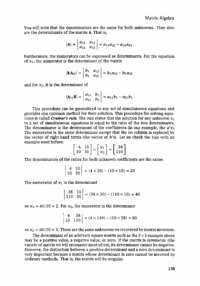
Matrix Algebra
You will note that the denominators are the same for both unknowns. They also are the determinants of the matrix A. That is,
Furthermore, the numerators can be expressed as determinants. For the equation of XI, the numerator is the determinant of the matrix
and for x2, it is the determinant of
This procedure can be generalized to any set of simultaneous equations and provides one common method for their solution. This procedure for solving equa- tions is called Cramer’s rule. The rule states that the solution for any unknown xi in a set of simultaneous equations is equal to the ratio of the two determinants. The denominator is the determinant of the coefficients (in our example, the a’s). The numerator is the same determinant except that the i t h column is replaced by the vector of right-hand terms (the vector of b’s). Let us check the rule with an
The denominators of the ratios for both unknown coefficients are the same:
1 1: i: 1 = (4 x 30) - ( l o x 10) = 20
The numerator of X I is the determinant
I110 38 301 lo = (38 x 30) - (110 x 10) = 40
so x1 = 40/20 = 2. For X Z , the numerator is the determinant
38 = (4 x 110) - (10 x 38) = 60 I10 1101
so x2 = 60/20 = 3. These are the same unknowns we recovered by matrix inversion. The determinant of an arbitrary square matrix such as the 3 x 3 example above
may be a positive value, a negative value, or zero. If the matrix is symmetric (the variety of matrix we will encounter most often), its determinant cannot be negative. However, the distinction between a positive determinant and a zero determinant is very important because a matrix whose determinant is zero cannot be inverted by ordinary methods. That is, the matrix will be singular.
139

Statistics and Data Analysis in Geology - Chapter 3
1 2 3 4 5 6 2 4 6
What circumstances will lead to singularity? The condition indicates that two or more rows (or columns) of the matrix are linear combinations or linear transfor- mations of other rows; that is, the values in some rows (or columns) are dependent on values in other rows. For example, the determinant
= O
1 2 3 4 5 6 5 7 9
is zero because the third row of the matrix is simply twice the first row. Similarly, the determinant
= O
is zero because the third row is the s u m of rows one and two. Of course, in real problems the source of singularity usually is not so obvious. Consider the data in file BAL,TIC.TXT, which gives the weight-percent of sand in five successive size fractions, measured on bottom samples collected in an area of the Baltic Sea. We can calculate correlations between the five sand size categories and place the results in a square, symmetric correlation matrix:
I 1 0.243 -0.301 0.096 -0.261 0.243 1 -0.969 -0.562 -0.422
-0.301 -0.969 1 0.340 0.253 0.096 -0.562 0.340 1 0.691
-0.261 -0.422 0.253 0.691 1
It is not obvious that this matrix should be singular with a zero determinant, yet it is. The linear dependence comes about because the weight-percentages in the five size categories sum to 100 for each observation, so there are induced negative correlations between the size categories. (Actually, because of rounding during computations, you may compute a correlation matrix that is not exactly singular. Depending upon the numerical precision of the computer program, rather than exactly 0, you may observe a very small determinant such as -0.0002. A matrix with a determinant near zero is said to be ill-conditioned.)
Finally, there is another special case of interest. An identity matrix has a de- terminant equal to 1.0. If several variables are completely independent of each other, their correlations will be near zero and they will form a correlation matrix that approximates an identity matrix. The determinant of such a matrix will be close to one, and its logarithm will be close to zero; this is the basis for one test of independence between variables.
140
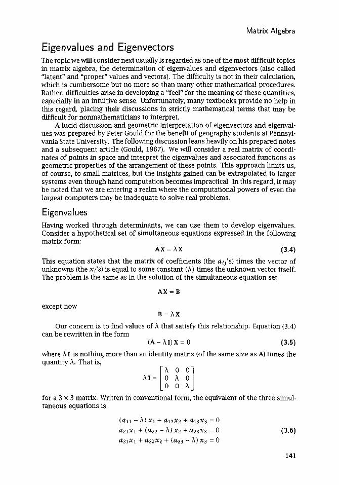
Matrix Algebra
E igenva I u es a n d E igenvect ors The topic we will consider next usually is regarded as one of the most difficult topics in matrix algebra, the determination of eigenvalues and eigenvectors (also called “latent” and “proper” values and vectors). The difficulty is not in their calculation, which is cumbersome but no more so than many other mathematical procedures. Rather, difficulties arise in developing a “feel” for the meaning of these quantities, especially in an intuitive sense. Unfortunately, many textbooks provide no help in this regard, placing their discussions in strictly mathematical terms that may be difficult for nonmathematicians to interpret.
A lucid discussion and geometric interpretation of eigenvectors and eigenval- ues was prepared by Peter Gould for the benefit of geography students at Pennsyl- vania State University. The following discussion leans heavily on his prepared notes and a subsequent article (Gould, 1967). We will consider a real matrix of coordi- nates of points in space and interpret the eigenvalues and associated functions as geometric properties of the arrangement of these points. This approach limits us, of course, to small matrices, but the insights gained can be extrapolated to larger systems even though hand computation becomes impractical. In this regard, it may be noted that we are entering a realm where the computational powers of even the largest computers may be inadequate to solve real problems.
Eigenva I ues Having worked through determinants, we can use them to develop eigenvalues. Consider a hypothetical set of simultaneous equations expressed in the following matrix form:
This equation states that the matrix of coefficients (the Ui j ’S ) times the vector of unknowns (the xi’s) is equal to some constant ( A ) times the unknown vector itself. The problem is the same as in the solution of the simultaneous equation set
A X = A X (3.4)
A X = B
except now B = h X
Our concern is to find values of h that satisfy this relationship. Equation (3.4) can be rewritten in the form
(A - h I ) X = 0
where h I is nothing more than an identity matrix (of the same size as A) times the quantity A. That is,
(3.5)
h I = 0 h 0 [: : :] for a 3 x 3 matrix. Written in conventional form, the equivalent of the three simul- taneous equations is
(all - h ) x1 + d12x2 + d.13x3 = 0
141

Statistics and Data Analysis in Geology - Chapter 3
IA-hII=
Let us assume that there are solutions to these equations other than the trivial case where all the unknown x’s = 0. Look back at Cramer’s rule for the solution of simultaneous equations, in which the unknowns are expressed as the ratio of two determinants. Because the numerator in our present example would contain a column of zeros, the determinant of the numerator also will be zero. That is, the solution for the X vector is
x = - 0 IAl
all - a12 a13 a21 a22-h a23 = O (3.8) a3 1 a32 a33-
Rewriting, this becomes I A l X = O (3.7)
Thus we have
Because we know the various values of the elements aij, we can collect all of these terms together in the form of an equation such as
where the (x’s represent the sum of the numerical values of the appropriate aij’s. You should recognize that this is a quadratic equation of the general form
ax2 + bx + c = 0
which can be solved for the unknown terms by factoring. The general solution to a quadratic equation is
(3.10) -b+- X = 2a
142

Matrix Algebra
If this seems unfamiliar, review the sections in an elementary algebra book that deal with factoring and quadratic equations. Now, we can try the procedures just outlined to find the eigenvalues of the 2 x 2 matrix:
A = [17 45 -16 -"] First, we must set the matrix in the form
Equating the determinant to zero,
-6 l = o 1 1 7 4 45 -16-h
we can expand the determinant
Multiplying out gives
-272 - 17h + 16h + h2 + 270 = 0
which can be collected to give
This can be factored into
A 2 - h - 2 = 0
(A - 2) ( A + 1) = 0
So, the two eigenvalues associated with the matrix A are
This example was deliberately chosen for ease in factoring. We can try a some- what more difficult example by using the set of simultaneous equations we solved earlier. This is the 2 x 2 matrix:
A = [ ''1 10 30
Repeating the sequence of steps yields the determinant
which is then expanded into
I 4c; 3:! 1 = (4 - A ) (30 - A ) - 100 = 0
143

Statistics and Data Analysis in Geology- Chapter 3
or h2 - 34h + 20 = 0
There are no obvious factors in the quadratic equation, so we must apply the rule for a general solution:
- (-34) c J-342 - 4 x 1 x 20 34 + J iDZ 2
- = A = - - b + J- X =
2 a 2 x 1
hi = 33.4 A2 = 0.6
We can check our work by substituting the eigenvalues back into the determi- nant to see if it is equal to zero, within the error introduced by round-off
So, the eigenvalues we have found are correct within two decimal places. Before we leave the computation of eigenvalues of 2 x 2 matrices, we should
consider one additional complication that may arise. Suppose we want the eigen- values of the matrix
A = [ -6 2 41 3
Expressed as a determinant equal to zero, we have
which expands to
or
The roots of this equation are
h2 - 5 h + 30 = 0
But this leads to equations involving the square roots of negative numbers:
= 2.5 + 4.9i 5 + m 2
hl =
= 2 . 5 - 4.9i 5 - m 2 A2 =
144

Matrix Algebra
2 0 - h -4 8 -40 8 - h -20 -60 12 - 2 6 - h
These are complex numbers, containing both real parts and imaginary parts which include the imaginary number, i = a. Fortunately, a symmetric matrix always yields real eigenvalues, and most of our computations involving eigenvalues and eigenvectors will utilize covariance, correlation, or similarity matrices which are always symmetrical.
Next, we will consider the eigenvalues of the third-order matrix:
= O
20 -4 [ -40 8 -2:] -60 1 2 -26
Expanding out the determinant and combining terms yields
-A3 + 2h2 + 8h = 0
This is a cubic equation having three roots that must be found. In this instance, the polynomial can be factored into
( A - 4) ( A - 0 ) ( A + 2) = 0
and the roots are directly obtainable:
h 1 = + 4 h2=O & = - 2
Although the techniques we have been using are extendible to any size matrix, finding the roots of large polynomial equations can be an arduous task. Usually, eigenvalues are not found by solution of a polynomial equation, but rather by ma- trix manipulation methods that involve refinement of a successive series of approx- imations to the eigenvalues. These methods are practical only because of the great computational speed of digital computers. Utilizing this speed, a researcher can compress literally a lifetime of trial solutions and refinements into a few minutes.
We can now define another measure of the “size” of a square matrix. The rank of a square matrix is the number of independent rows (or columns) in the matrix and is equal to the number of nonzero eigenvalues that can be extracted from the matrix. A nonsingular matrix has as many nonzero eigenvalues as there are rows or columns in the matrix, so its rank is equal to its order. A singular matrix has one or more rows or columns that are dependent on other rows or columns, and consequently will have one or more zero eigenvalues; its rank will be less than its order.
Now that we have an idea of the manipulations that produce eigenvalues, we may try to get some insight into their nature. The rows of a matrix can be regarded as the coordinates of points in m-dimensional space. If we restrict our considera- tion to 2 x 2 matrices, we can represent this space as an illustration on a page and can view matrix operations geometrically.
145
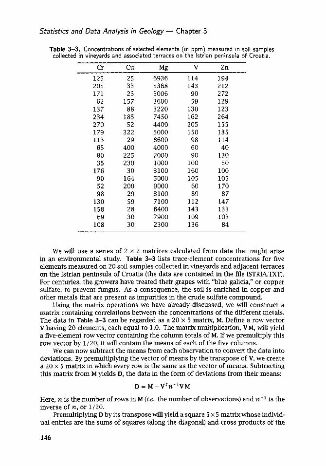
Statistics and Data Analysis in Geology - Chapter 3
Table 3-3. Concentrations of selected elements (in ppm) measured in soil samples collected in vineyards and associated terraces on the lstrian peninsula of Croatia.
Cr cu Mg V Zn 1 2 5 25 205 33 171 25 62 157
137 88 2 34 185 2 70 52 179 322 113 29 65 400 80 225 35 230
176 30 90 164 52 200 98 29
130 59 158 28 69 30
108 30
6936 5368 5006 3600 3220 7450 4400 5000 8600 4000 2000 1000 3100 5000 9000 3 100 7100 6400 7900 2300
114 194 143 212 90 2 72 59 129
130 123 162 2 64 205 155 150 135 98 114 60 40 90 130
100 50 160 100 105 105
60 170 89 87
112 147 143 133 109 103 136 84
We will use a series of 2 x 2 matrices calculated from data that might arise in an environmental study. Table 3-3 lists trace-element concentrations for five elements measured on 20 soil samples collected in vineyards and adjacent terraces on the Istrian peninsula of Croatia (the data are contained in the file 1STRIA.TXT). For centuries, the growers have treated their grapes with “blue galicia,” or copper sulfate, to prevent fungus. As a consequence, the soil is enriched in copper and other metals that are present as impurities in the crude sulfate compound.
Using the matrix operations we have already discussed, we will construct a matrix containing correlations between the concentrations of the different metals. The data in Table 3-3 can be regarded as a 20 x 5 matrix, M. Define a row vector V having 20 elements, each equal to 1.0. The matrix multiplication, V M , will yield a five-element row vector containing the column totals of M. If we premultiply this row vector by 1 /20, it will contain the means of each of the five columns.
We can now subtract the means from each observation to convert the data into deviations. By premultiplying the vector of means by the transpose of V, we create a 20 x 5 matrix in which every row is the same as the vector of means. Subtracting this matrix from M yields D, the data in the form of deviations from their means:
D = M - V T n - l V M
Here, n is the number of rows in M (te., the number of observations) and n-l is the inverse of n, or 1/20.
Premultiplying D by its transpose will yield a square 5 x 5 matrix whose individ- ual entries are the sums of squares (along the diagonal) and cross products of the
146

Matrix Algebra
five elements, corrected for their means. If we divide a corrected sum of squares by n - 1 we obtain the variance, and if we divide a corrected sum of products by n - 1 we obtain the covariance. These are the elements of the covariance matrix, S, which we can compute by
s = (n - i 1 - l ~ ~ ~
A subset of S could serve our purposes (and the covariance matrix often is used in multivariate statistics), but the relationships will be clearer if we use the correlation matrix, R. Correlations are simply covariances of standardized variables; that is, observations from which the means have been removed and then divided by the standard deviation. In matrix D, the means have already been removed. We can, in effect, divide by the appropriate standard deviations if we create a 5 x 5 matrix, C, whose diagonal elements are the square roots of the variances found on the diagonal of S, and whose off-diagonal elements are all 0.0. If we invert C and premultiply by D, each element of D will be divided by the standard deviation of its column. Call the result U, a 20 x 5 matrix of standardized values;
U = DC-’
We can calculate the correlation matrix by repeating the procedure we used to find S, substituting U for D:
R = (n - l ) - l U T U
1 1 0.595 -0.28 0.456 0.242 1
1 -0.312 0.141 0.85 0.595 -0.312 1 -0.201 -0.33 -0.28
R = 0.141 -0.201 1 -0.029 0.456 0.85 -0.33 -0.029 1 0.242
To graphically illustrate matrix relationships, we must confine ourselves to 2 x 2 matrices, which we can extract from R. Copper and zinc are recorded in the second and fifth columns of M, and so their correlations are the elements Yi,j whose subscripts are 2 and 5:
1 Rcu,,.,, = [ Y 2 1 2 “ g 5 ] = [ 1 -0.28 r5,2 r5,S -0.28 1
If we regard the rows as vectors in X and Y , we can plot each row as the tip of a vector that extends from the origin. In Figure 3-1, the tip of each vector is indicated by an open circle, labeled with its coordmates. The ends of the two vectors lie on an ellipse whose center is at the origin of the coordinate system and which just encloses the tips of the vectors. The eigenvalues of the 2 x 2 matrix R,,,,, represent the magnitudes, or lengths, of the major and minor semiaxes of the ellipse. In this example, the eigenvalues are
hi = 1.28 A2 = 0.72
Gould refers to the relative lengths of the semiaxes as a measure of the “stretch- ability” of the enclosing ellipse. The semiaxes are shown by arrows on Figure 3-1. The first eigenvalue represents the major semiaxis whose length from center to
147

Statistics and Data Analysis in Geology - Chapter 3
1 .o: -
-0.28, 1 I 1 .o:
-
3
-0.28, 1
Figure 3-1. Ellipse defined by rows in matrix of correlations between copper and zinc. Eigenvectors of matrix correspond to principal semiaxes (arrows) of ellipse.
-2.0-,,
edge of the ellipse is 1.28 units. The second eigenvalue represents the length of the minor semiaxis, which is 0.72 units.
If the two vectors are closer together, the ratio between the semiaxes of the enclosing ellipse will change. For example, chromium and vanadium have very similar behavior in the vineyard soil samples, leading to a high correlation between the two. Their correlations are given by elements in the first and fourth rows and
I , , , , , , I I , , , , , , , , I , , 4 I I I I I I I I I I , , , , I
The rows of RCY,,, are plotted as vectors in Figure 3-2. The eigenvalues of this 2 x 2 matrix are
hi = 1.85 hz = 0.15
-2.0-,,
which define one very long major semiaxis and a short minor semiaxis. At the limit, we can imagine that two variables might behave in an identical fashion. Then, their rows in R would be so similar that they would be identical and the plotted vectors would coincide. That is,
I , , , , , , I I , , , , , , , , , I 4 I I I I I I I I I I , , , , I
The enclosing ellipse would collapse to a straight line of semiaxis length hl = 2 and a minor semiaxis of hz = 0.
At the opposite extreme, two variables which are completely unrelated will have a correlation of near zero. Magnesium and vanadium show such behavior in the vineyard samples. They are represented by elements in the third and fourth rows and columns of R, and are shown plotted as vectors in Figure 3-3.
148

Matrix Algebra
3
Figure 3-2. Elongated ellipse defined by rows in matrix of correlations between chromium and vanadium, which are highly correlated.
2’o-:
-2.0 -2.0 -1 .o .O 1 .o 2
MG 0
Figure 3-3. Nearly circular ellipse defined by rows in matrix of correlations between mag- nesium and vanadium, which have a correlation approaching zero.
The two eigenvalues of this matrix are
hi = 1.029 A2 = 0.971
which are almost identical in size. As we can see, they define the major and minor semiaxes of an ellipse that is almost a circle, and both the semiaxes and the vectors are essentially radii. By definition, the axes of the ellipse are at right angles to each other, and the two plotted vectors also are almost orthogonal.
Some final notes on eigenvalues: You’ll notice that the correlation matrices we’ve graphed are square, symmetrical about their diagonals, composed of real elements (that is, no imaginary numbers), and that the largest numbers in every row
149

Statistics and Data Analysis in Geology - Chapter 3
are on the diagonal. As a consequence of these special conditions, the eigenvalues will always be real numbers that are equal to or greater than zero. As you can verify by checlung these examples, the sum of the eigenvalues of a matrix is always equal to the sum of the diagonal elements, or the trace, of the original matrix. In a correlation matrix, the diagonal elements are all equal to one, so the trace is simply the number of variables. The product of the eigenvalues will be equal to the determinant of the original matrix. Most (but not all) of the eigenvalue operations we will consider later will be applied to correlation or covariance matrices, so these special results will hold true in most instances. The methods just developed can be extended directly to n x n matrices, although the procedure becomes increasingly cumbersome with larger matrices.
E igenvect ors We can examine the correlation matrices we calculated for the Istrian vineyard data to gain some insight into the geometrical nature of eigenvectors. First, consider the 2 x 2 matrix
with eigenvalues A1 = 1.28 A2 = 0.72
Substituting the first eigenvalue into the original matrix gives
1 1 - 1.28 -0.28 ] = [ -0.28 -0.28 -0.28 1 - 1.28 -0.28 -0.28
whose solution is the eigenvector
[ 4 = [ -:] In Figure 3-1, we can interpret this eigenvector as the slope of the major semi-
axis of the enclosing ellipse. If we regard the elements of the eigenvector as coor- dinates, the first eigenvector defines an axis whch extends from the center of the ellipse into the second quadrant at an angle of 135". The length is equal to the first eigenvalue, or 1.28.
Turning to the second eigenvalue, A2 = 0.72, the equation set is
1 1 - 0.72 -0.28 ] = [ 0.28 -0.28 -0.28 1 - 0.72 -0.28 0.28
whose solution gives the second eigenvector:
[::I = [ :] In Figure 3-1, t h s will plot as the vector drection l / l = 45", perpendicular to the major semiaxis of the ellipse. Its magnitude or length is 0.72.
150

Matrix Algebra
We can determine the eigenvalues for the matrix of correlations between chro- mi= and vanadium in a similar fashion. The matrix is
with eigenvalues hi = 1.85 A2 = 0.15
The first eigenvector is
1 - 1.85 0.85 1 = 1-0.85 0.85 1 1 0.85 1 - 1.85 0.85 -0.85 L A L A
[::I = [:I which defines a line having a slope of 45". This axis bisects the angle between the two points and the center of the ellipse in Figure 3-2. The magnitude of the major semiaxis is equal to 1.85, the first eigenvalue of RC7,,,. Similarly, we can show that the eigenvector associated with th( second eigenvalue is
1-0.15 0.85 ] = [ 0.85 0.851 0.85 1 - 0.15 0.85 0.85
[ ::I = [-:I This procedure can be applied to the matrix Rmg,,, and the eigenvectors found
will again define directions of 135" and 45", as shown in Figure 3-3. By now you no doubt suspect that the eigenvectors of 2 x 2 symmetric matrices will always lie at these specific angles, and this is indeed the case. The eigenvectors of real, symmetric matrices are always orthogonal, or at right angles to each other. This is not true of eigenvectors of matrices in general, but only of symmetric matrices. In addition, the eigenvectors of two-dimensional symmetric matrices are additionally constrained to orientations that are multiples of 45". Incidentally, if two vectors, A and B, are orthogonal, then ATB = 0.
Eigenvalue and eigenvector techniques are directly extendible to larger matri- ces, even though the operations become tedious. As an example, we will consider the full 5 x 5 correlation matrix R for trace metals from Istrian vineyard soils. The five eigenvalues of this matrix are
A = 12.453 1.233 0.789 0.465 L
and their associated eigenvectors are
0.585 -0.363
0.498 0.469
-0.248 -0.075
Vp = [ 0.736
0.389 -0.490
0.259 0.95 1
0.052 0.300
v4 =
0.061 ]
1::!::] [ -0.727 0.062
-0.628 Vs = -0.023 -0.398 0.593
0.652 0.339
151

Statistics and Data Analysis in Geology - Chapter 3
Each eigenvector can be regarded as a set of coordinates in five-dimensional space that defines the “direction” of a semiaxis of a hyperellipsoid. The length of each semiaxis is given by the corresponding eigenvalue. The first semiaxis is twice as long as the second, which is almost twice the length of the third. The fourth axis is very short, and the fifth axis is almost nonexistent; the hyperellipse defined by the correlation matrix, R, is really only a three-dimensional disk embedded in a space of five dimensions.
The slope of a line drawn from the origin of a graph through a point is defined by the ratio between the two coordinates of the point, and not by the actual mag- nitudes of the coordinates. Similarly, the absolute magnitudes of the elements in eigenvectors are not significant, only the ratios between the elements. An eigen- vector can be scaled by multiplying by any arbitrary constant, and it will still define the same direction in multidimensional space. Different computer programs may return different eigenvectors for the same matrix; the eigenvectors simply have been scaled in different ways. Most programs normalize, or scale each eigenvector so the sum of the squares of each element in a vector will be equal to 1.0. Others scale each eigenvector so the sum of its elements will be equal to its eigenvalue. Although such results appear to be different, the ratios between pairs of elements in the eigenvectors remain the same, and the vectors they define point in the same “direction.” Also, you may note that the pattern of signs on the elements of the eigenvectors seems to be different for two otherwise identical sets of eigenvectors. This merely means that one set of vectors has been multiplied by (-l), reversing its “direction” but not changing its orientation in multivariate space.
Increasingly, computer programs for multivariate analysis employ alternative techniques for obtaining eigenvalues and eigenvectors. Rather than reducing a rect- angular data matrix to a symmetrical, square correlation or covariance matrix and then extracting the desired eigenvalues and eigenvectors as we have done, these programs obtain results directly from the data matrix by singular value decom- position (SVD). An excellent description of SVD is given by Jackson (1991); Press and others (1992) provide a more compact presentation, as well as computer pro- gram listings. We will delay a discussion of this procedure until Chapter 6, where we can provide a motivation for our interest. Now, we merely note that an n x m rectangular matrix, X, can be decomposed into three other matrices:
where W contains the eigenvectors of the major product matrix, XXT. V contains the eigenvectors of the minor product matrix, XTX, and A is an m x m diagonal matrix whose diagonal elements are the eigenvalues of either XXT or XTX (they will be identical except that XTX will have n - m extra eigenvalues, all equal to zero).
If you have worked through the small examples in this chapter, you can readily appreciate that the computational labor involved in dealing with large matrices can be formidable, even though the underlying, individual mathematical steps are sim- ple. A modest data set such as 1STRIA.m will present a challenge to those who attempt to analyze the data by hand. Fortunately, there are many powerful compu- tational tools available at modest cost (at least for student versions), and they run on almost any type of personal computer. A numerical computation package such as MATLAB@, Mathcad@, or MATHEMATICA@, and even some statistical packages,
152

Matrix Algebra
such as S-PLUS@ , will provide all of the mathematical computation power you are likely to need for applications in the Earth sciences. We have attempted to present, in as painless a manner as possible, the rudiments of beginning matrix algebra. As stated at the conclusion of Chapter 2, statistics is too large a subject to be covered in one chapter, or even one book. Matrix algebra also is an impossibly large subject to encompass in these few pages. However, you should now have some insight into matrix methods that will enable you to understand the computational basis of techniques we will cover in the remainder of this book.
EXERCISES
Exercise 3.1 File BHTEMP.TXT contains 15 bottomhole temperatures (BHT’s) measured in the Mississippian interval in wells in eastern Kansas. The measurements are in degrees Fahrenheit. Convert the vector of temperatures to degrees Celsius using matrix algebra.
Exercise 3.2 The following two matrices are defined:
A = [ -2 0 ‘1 B = [ - 3 -2 -4 ‘1 Compute the matrix products, A B and B A. Two matrices which exhibit the property that will be apparent are said to be commutative. Demonstrate that for commuta- tive matrices, A - ~ B - ~ = (ABP
Consider the following two matrices,
2 1 0 1 -1 c = [o 3 4 0 0 2 ] .= [ : : i ]
Compare the determinant, (CDI, of the matrix product to the product, (CI - IDI, of the determinants of the two matrices. The result you obtain is general. Deter- mine if ICI + ID( = IC + DI. This result also is general. For the matrices C and D, demonstrate that (CD)T = DTCT. Using matrix C, show that (C-l)T = (CT)-l.
Exercise 3.3 File MAGNET1T.m contains the proportions of olivine, magnetite, and anorthite estimated by point-counting thin sections from 15 hand specimens collected at a magnetite deposit in the Laramie Range of Wyoming. The specific gravity is 3.34 for olivine, 2.76 for anorthite, and 5.20 for magnetite. Using matrix algebra, estimate the specific gravity of the 15 samples.
153

Statistics and Data Analysis in Geology - Chapter 3
Exercise 3.4 Coordinates can be rotated by a matrix multiplication in which the premultiplier is a 2 x 2 matrix of sines and cosines of the angle of rotation,
I C O S ~ sine [ - s ine c o ~ e
where 8 is the desired angle of rotation. Data in file PROSPECT.TXT were taken from a surveyor's notebook describing the outline of a gold prospect in central Idaho. Coordinates are given in meters from an arbitrary origin at the southwest corner of the property and were measured relative to magnetic north. The magnetic declina- tion in this area is 18'30' east of true north. Convert the surveyor's measurements to coordinates relative to true north.
Exercise 3.5 Petrophysical well logs are strip charts made after the drilling of a well by lowering a sonde down the hole and recording physical properties versus depth in the well. Measurements include various electrical and sonic characteristics of the rocks, and both natural and induced radioactivity. The measured values reflect the composi- tion of the rocks and the fluids in the pore space.
File KANSALT.TXT contains data for depths between 980 and 1 0 3 0 ft below the surface in A.E.C. Test Hole No. 2, drilled in 1 9 7 0 in Rice County, Kansas. At this depth, the well penetrated the Hutchinson Salt member of the Permian Wellington Formation, which was under investigation as a possible nuclear waste disposal site. The Wellington Formation is composed entirely of varying proportions of halite, an- hydrite, and shale. Pure samples of these end members have distinct physical prop- erties, so appropriate log responses can be used to estimate the relative amounts of halite, anhydrite, or shale at every foot within the Wellington Formation. A more detailed discussion of these data is given in Doveton (1986).
Table 3-4. Physical properties measured on pure samples of halite, anhydrite, and "shale" (clay minerals). From Gearhart-Owen (1975).
Halite Anhydrite Shale
Apparent grain density ( P b ) , g/cc 2.03 2 .98 2 .43
Sonic transit time (At) , psec/ft 67 5 0 1 1 3
Two useful petrophysical properties are the apparent density (in grams per cubic centimeter) as measured by gamma-ray absorption and sonic transit time (in microseconds per foot). Laboratory-determined values for pure halite, anhydrite, and shale are given in Table 3-4. The apparent density and the sonic transmis- sion time of a mixture of these three constituents can be calculated as the sum of the products of the densities and transit times for pure constituents times the proportions of the constituents. That is,
P b = 2.03Vh + 2.98Va -?- 2.43vsh
At = 67Vh + SOVa + 113vsh
154

Matrix Algebra
where vh, V,, and Vsh are the proportions of halite, anhydrite, and shale. However, we want to reverse these equations, and for given values of P b and At that we read from the well logs, estimate the proportions of the three constituents of the rock. Since three unknowns must be estimated, it seems we will require three equations and, hence, measurements of three log properties. However, because the proportions of halite, anhydrite, and shale must sum to one, we can use this constraint to provide the necessary third equation.
The three equations can be set into matrix form as
L = cv [:I=[ 2.03 7 2.98 2.43 1;3] [va v h
Vsh
However, what we really want to do is solve for V, given values of L taken from the well logs. This means that C must be moved to the other side of the equal sign, which we can do by multiplying both sides of the equation by its inverse, C - l . Then,
[ 2.03 y 2.98 y 2.43 y 1 - l [;I]-[ 21 Vsh
Perform the necessary matrix inversion and multiplications to determine the proportions of halite, anhydrite, and shale in the 50-ft interval of the Hutchinson Salt. Plot the record of lithologic compositions in the form of a lithologic strip log. Ten of these estimates have been used in Chapter 2 (Table 2.9) to demonstrate the effects of closure on the calculation of correlations among closed variables. [Hint: L, as given in file KANSALT.TXT, is a 2 x 50 matrix of P b and At log responses. It must be converted to a 3 x 50 matrix by adding a column of 1’s in order for the dimensions of the matrix multiplication to be correct. What does this column of 1’s represent?]
Exercise 3.6 The state of stress in the subsurface can be represented in a 3 x 3 matrix, Z, whose diagonal elements represent normal stresses and whose off-diagonal elements rep- resent shear stresses. The meanings of the nine elements of the stress matrix can be seen by imagining a cube in a Cartesian coordinate system in which the X-axis points to the east, the Y-axis points to the north, and the Z-axis points up. The symbol axx represents the normal stress directed onto the east or west face of the cube; it will be a positive value if the stress is compressional and a negative value if the stress is tensional. There is a similar meaning for ayy and aZz. The symbol a,, represents the shear stress on the east or west face of the cube, acting parallel to the Y-axis. A shear stress is positive if the compressional or tensional compo- nent agrees in sign with the direction of force. That is, both components of shear
155

Statistics and Data Analysis in Geology- Chapter 3
point in a positive coordinate direction, or both components point in a negative coordinate direction. Otherwise, the shear stress is negative. In order for the cube to be in rotational equilibrium, shear stresses on adjacent faces must balance; so, for example, uxy = urx. This means that the stress matrix is symmetric about the diagonal:
Turcotte and Schubert (1982) provide a more detailed discussion of stress in the subsurface and the measurement of stress components.
By finding the eigenvalues and eigenvectors of the 3 x 3 stress matrix, we can rotate the imaginary cube into a coordinate system in which all the shear stresses will be zero. The eigenvalues represent the magnitudes of the three orthogonal stresses. Their associated eigenvectors point in the directions of the stresses. The largest eigenvalue, h l , represents the maximum normal stress and the smallest, h3, represents the minimum normal stress. The maximum shear stress is given by (Al - h3) /2 and occurs along a plane oriented perpendicular to a line that bisects the angle between the directions of maximum and minimum normal stress (that is, between the first and third eigenvectors). In a homogenous, isotropic material, failure ( t e . , faulting) will tend to occur along this plane. The orientation of this plane can be determined from the elements of the first eigenvector. In the conventional notation used by geologists, the strike of the first eigenvector is tan-l ( Y ~ z / Y I ~ ) and its dip is
(Here, Vij refers to the j t h element of the i t h eigenvector.) The strike and dip of the second and third eigenvectors can be found in the same manner.
Three-dimensional stress measurements have been made in a pillar in a deep mine, yielding the following stress matrix:
1 61.2 4.1 -8.2 4.1 51.5 -3.0
-8.2 -3.0 32.3
The data are given in megapascals (MPa) and were recorded by strain gauges placed so the measurements have the same orientation as our imaginary cube ( X increasing to the east, Y to the north, and Z increasing upward). Find the principal stresses and their associated directions. What is the maximum shear stress and what is the strike and dip of the plane on which this stress occurs?
156

Matrix Algebra
SELECTED READINGS
Anton, H., and C. Rorres, 1994, Elementary Linear Algebra, 7th ed., Applications Version: John Wiley & Sons, Inc., New York, 800 pp. A computationally ori- ented text on matrix algebra. Diskeffes contain examples and exercises.
Buchanan, J.L., and P.R. Turner, 1992, Numerical Methods and Analysis: McGraw- Hill, Inc., New York, 751 pp.
Davis, P.J., 1984, The Mathematics ofMatrices: R.E. Krieger Publ. Co., Malabar, Fla., 368 pp. Reprint of a classic. A highly readable text on matrix algebra with a minimum of mathematicaljargon and a maximum of examples and applications.
Doveton, J.H., 1986, Log Analysis o f Subsurface Geology: Concepts and Computer Methods: John Wiley & Sons, Inc., New York, 273 pp. Chapter 6 discusses matrix algebra techniques for resolving rock composition from well log responses, including the Hutchinson Salt (file KANSALT: TXT) exercise.
Ferguson, J., 1988, Mathematics in Geology: Allen & Unwin Ltd., London, 299 pp. Chapters 6 and 7 treat matrix algebra and its application to geological problems.
Gearhart-Owen, 1975, Formation Evaluation Data Handbook: Gerhard-Owen Indus- tries, Inc., Fort Worth, Texas, 240 pp.
Golub, G.H., and C.F. Van Loan, 1996, Matrix Computations, 3Td ed.: Johns Hopkins Univ. Press, Baltimore, Md., 694 pp.
Gould, P., 1967, On the geographic interpretation of eigenvalues: An initial explo- ration: Trans. Inst. British Geographers, No. 42, p. 53-86. An intuitive look at eigenvalues and vectors by geometric analogy. Part of this chapter is derived from this excellent exposition, wrlffen originally for students.
Jackson, J.E., 1991, A User's Guide to Principal Components: John Wiley & Sons, Inc., New York, 569 pp. Appendices A and B are a concise summary of matrix algebra. Chapter 10 discusses singular value decomposition.
Jensen, J.A., and J.H. Rowland, 1975, Methods o f Computation: The Linear Approach to Numerical Analysis: Scott, Foresman and Co., Glenview, Ill., 303 pp.
Maron, M.J., and R.J. Lopez, 1991, Numerical Analysis-A Practical Approach, 37'd ed.: PWS-Kent Publ. Co., Boston, Mass., 743 pp. Gives procedures and algorithms for matrix operations, especially different methods for inversion, solution of simul- taneous equations, and extraction of eigenvalues.
Ortega, J.M., 1990, Numerical Analysis, a Second Course: Society for Industrial and Applied Mathematics, Philadelphia, Pa., 201 pp. A concise but complete text, issued as a paperback reprint b y SlAM to "foster beffer understanding of applied mathematics."
Pettofrezzo, A. J., 1978, Matrices and Transformations: Dover Publications, Inc., New York, 13 3 pp. This paperback reprint of a classic text covers the traditional ma- terial for a one-semester matrix algebra course. lt is liberally sprinkled with worked examples and problems.
157

Statistics and Data Analysis in Geology - Chapter 3
Press, W.H., S.A. Teukolsky, W.T. Vetterling, and B.P. Flannery, 1992, Numerical Recipes: The Art ofScienrific Computing, Znd ed.: Cambridge Univ. Press, Cam- bridge, U.K., 963 pp. The "how-to" book of computer algorithms for numerical computation; contains succinct descriptions of eigenvalue techniques, including SVD. Available in several versions for different computer languages.
Searle, S.R., 1982, Matrix Algebra Useful for Statistics: John Wiley & Sons, Inc., New York, 438 pp. Examples and exercises ure drawn from the biological sciences.
Turcotte, D.L., and G. Schubert, 1982, Geodynamics Applications of Continuum Phys- ics to Geological Problems: John Wiley & Sons, Inc., New York, 450 pp.
Wolfram, S., 1996, The MATHEMATICAB Book: Wolfram Media, Inc., Champaign, Ill., 1395 pp.
158

In this chapter we will consider ways of examining data that are characterized by their position along a single line. That is, they form a sequence, and the posi- tion at which a data point occurs within the sequence is important. Data sets of this type are common in geology, and include measured successions of lithologies, geochemical or mineralogical assays along traverses or drill holes, electric logs of oil wells, and chart recordings from instruments. Also in this general category are measurements separated by the flow of time, such as a sequence of water quality determinations at a river station, or the production history of a flowing gas well. Techniques for examining data having a single positional characteristic tradition- ally are considered part of the field of time-series analysis, although we will take the broader view that time and space relationships can be considered interchangeably.
Geologic Measurements in Sequences Before proceeding to some geological examples and appropriate methods of ex- amination, we must consider the nature of different types of sequences apt to be encountered by geologists. At one extreme, we may have a record which is quite precise, both in the variable which is measured and in the scale along which suc- cessive observations are located. Examples might include an electrical resistivity log from a borehole, or the production history of a commercial well. In the for- mer, the variable is a measured attribute expressed in ohms (R) and the scale is measured in feet. In the latter example, the variable again is a measured attribute, barrels (bbl) of oil, and the scale is measured in days, months, or years. There are two important characteristics in either record. First, the variable being measured is expressed in units of an interval or ratio scale; 1000 bbl of oil is twice as large a quantity as 500 bbl, and a measurement of 10 R is ten times the resistance of 1 SZ. Second, the scales along which the data points are located also are expressed

Statistics and Data Analysis in Geology - Chapter 4
in units having magnitude. A depth of 3000 ft in a well is ten times a depth of 300 ft, and the decade between the years 1940 and 1950 has the same duration as the interval between 1950 and 1960. These may seem obvious or even trivial points to emphasize, but as we shall see, not all geologic sequences have such well-behaved characteristics.
At the opposite extreme, we can consider a stratigraphic sequence consisting of the lithologic states encountered in a sedimentary succession. Such a sequence might be a cyclothem of limestone-shale-limestone-shale-sandstone-coal-shale- limestone, from bottom to top. We are interested in the significance of the succes- sion, but we cannot put a meaningful scale on the sequence itself. Obviously, the succession of lithologies represents changes that occurred through time, but we have no way of estimating the time scale involved. We could use thickness, but this may change dramatically from location to location even though the sequence is not altered. If thickness is considered, it may obscure our examination of the succes- sion, which is the subject of our interest. Thus, the fact that limestone is the third state in the section and coal is the sixth has no significance that can be expressed numerically (that is, position 6 is not “twice” position 3). Likewise, the lithologic states of the units cannot be expressed on a numerical scale. We might code the sequences just given as 1 - 2 - 1 - 2 - 3 - 4 - 2 - 1, where limestone is equated to 1, shale is 2, sandstone is 3, and coal is 4, but such a convention is purely arbitrary and expresses no meaningful relations between the states. It is obvious that this sequence poses different problems to the analyst than do the first examples.
There also are intermediate possibilities. For example, we may be interested in some measurable attribute contained in successive stages of a sequence. Perhaps we have measured the boron content of each lithologic unit in the cyclothem just discussed. We can utilize a distance scale of feet between samples and consider this a problem related to depth or distance. Alternatively, we can consider the relationship between the boron measurements and the sequence of states.
A closely related problem is the analysis of a sequence characterized by the presence or absence of some variable or variables at points along a line. We might be interested, for example, in the repeated recurrence of certain environment- dependent microfossils in the chips recovered during the drilling of a well. Another class of problems may be typified by the succession of mineral grains encountered on traverses across a thin section. In this case, we can use millimeters as a conve- nient spatial scale, but we have no way of evaluating whether olivine rates a higher number than plagioclase.
Data having the characteristic of being arranged along a continuum, either of time or space, often are referred to as forming a series, sequence, string, or chain. The nature of the data and the chain determine the questions that we can consider. Obviously, we cannot extract information about time intervals from stratigraphic succession data, because the time scale accompanying the succession is not known. We often substitute spatial scales for a time scale in stratigraphic problems, but our conclusions are no better than our fundamental assumptions about the length of time required to deposit the interval we have measured.
Table 4-1 is a classification of the various data-analysis techniques discussed in this chapter. We can consider two types of sequences. In the first, the distance between observations varies and must be specified for every point. In the second, the points are assumed to be equally and regularly spaced; the numerical value of the spacing does not enter into the analyses except as a constant. A subset of
160

Analysis of Sequences of Data
Table 4-1. Techniques discussed in this chapter classified by the nature o f the variable and i ts spacing along a line. Locations are explicit if X is specified for
every Y ; locations are implicit if X is implied by the order o f observations.
Explicit Location Implicit Location Nature of Variables in Time or Space in Time or Space Interval or Ratio Data Interpolation Zonation
Regression Seriation Splines Autocorrelation
Cross-correlation Semivariograms Periodograms Spectral Density
Nominal or Ordinal Data Series of Events Markov Chains Runs Tests
this category does not consider the spacing at all, and only the sequence of the observations is important.
The techniques also may be classified on the type of observations they require. Some necessitate interval or ratio Observations; the variate must be measured on a scale and expressed in real numbers. Other methods accept nominal or ordinal data, and observations need only to be categorized in some fashion. In the methods discussed in this chapter, the classes are not ranked; that is, state A is not “greater” or “larger” in some sense than states B or C. Nominal data may be represented by integers, alphabetic characters, or symbols.
In the remainder of this chapter, we are going to examine the mathematical techniques required to analyze data in sequences. The methods described here do not exhaust the possibilities by any means. Rather, these are a collection of operations that have proved valuable in quantitative problem-solving in the Earth sciences, or that seem especially promising. Other methods may be more appropri- ate or powerful in specific situations or for certain data sets. However, a familiarity with the techniques discussed here will provide an introduction to a diverse field of analytical tools. Unfortunately, many of these methods were developed in scientific specialties alien to most geologists, and the description of an application in radar engineering, stock market analysis, speech therapy, or cell biology may be difficult to relate to a geologic problem. Some of the methods involve nonparametric statis- tics, and these are not widely considered in introductory statistics courses. Because of the general unfamiliarity of most Earth scientists with developments in the nu- merical analysis of data sequences, we have thought it best to present a potpourri of techniques and approaches. As you can see from Table 4.1, these cover a variety of sequences of different types, and are designed to answer different kinds of ques- tions. None of the techniques can be considered exhaustively in this short space, but from the examples and applications presented, one or another may suggest themselves to the geologist with a problem to solve. The list of Selected Readings can then provide a discussion of a specific subject in more detail.
These methods provide answers to the following broad categories of questions: Are the observations random, or do they contain evidence of a trend or pattern? If a trend exists, what is its form? C a n cycles or repetitions be detected and measured?
161
Statistics and Data Analysis in Geology - Chapter 4
Can predictions or estimations be made from the data? Can variables be related or their effectiveness measured? Although such questions may not be explicitly posed in each of the following discussions, you should examine the nature of the methods and think about their applicability and the type of problems they may help solve. The sample problems are only suggestions from the many that could be used.
Geologists are concerned not only with the analysis of data in sequences, but also with the comparison of two or more sequences. An obvious example is strati- graphic correlation, either of measured sections or petrophysical well logs. A ge- ologist's motive for numerical correlation may be a simple desire for speed, as in the production of geologic cross-sections from digitized logs stored in data banks. Alternatively, he may be faced with a correlation problem where the recognition of equivalency is beyond his ability. Subtle degrees of similarity, too slight for unaided detection, may provide the clues that will allow him to make a decision where none is otherwise possible. Numerical methods allow the geologist to consider many variables simultaneously, a powerful extension of his pattern-recognition facilities. Finally, because of the absolute invariance in operation of a computer program, mathematical correlation provides a challenge to the human interpreter. If a geol- ogist's correlation disagrees with that established by computer, it is the geologist's responsibility to determine the reason for the discrepancy. The forced scrutiny may reveal complexities or biases not apparent during the initial examination. This is not to say that the geologist should unthinkingly bend his interpretation to con- form with that of the computer. However, because modern programs for automatic correlation are increasingly able to mimic (and extend) the mental processes of a human interpreter, their output must be considered seriously.
Most techniques for comparing two or more sequences can be grouped into two broad categories. In the first of these, the data sequences are assumed to match at one position only, and we wish to determine the degree of similarity between the two sequences. An example is the comparison of an X-ray diffraction chart with a set of standards in an attempt to identify an unknown mineral. The chart and standards can be compared only in one position, where intensities at certain angles are compared to intensities of the standards at the same angles. Nothing is gained, for example, by comparing X-ray intensity at 20'28 with the intensity at 30'28 on another chart. Although the correspondence may be high, it is meaningless.
The fact that data such as these are in the form of sequences is irrelevant, because each data point is considered to be a separate and distinct variable. The intensity of diffracted radiation at 20'28 is one variable, and the intensity at 30"28 is another. We will consider methods for the comparisons of such sequences in greater detail in Chapter 6, when we discuss multivariate measures of similarity and problems of classification and discrimination. In this class of problems, an ob- servation's location in a sequence merely serves to identify it as a specific variable, and its location has no other significance.
In contrast, some of the techniques we will discuss in this chapter regard data sequences as samples from a continuous string of possible observations. There is no a pn'ori reason why one position of comparison should be better than any other. These methods of cross comparison superficially resemble the mental pro- cess of geologic correlation, but have the limitation that they assume the distance or time scales of the two sequences being compared are the same. In historic time series and sequences such as Holocene ice cores, this assumption is valid. In other
162

Analysis of Sequences of Data
circumstances such as stratigraphic correlation, equivalent thicknesses may not represent equivalent temporal intervals and the problem of cross comparison is much more complex.
As we emphasized in Chapter 1, the computer is a powerful tool for the anal- ysis of complex problems. However, it is mindless and will accept unreasonable data and return nonsense answers without a qualm. A bundle of programs for ana- lyzing sequences of data can readily be obtained from many sources. If you utilize these as a “black box” without understanding their operation and limitations, you may be led badly astray. It is our hope in this chapter that the discussions and examples will indicate the areas of appropriate application for each method, and that the programs you use are sufficiently straightforward so that their operation is clear. However, in the final analysis, the researcher must be his own guide. When confronted with a problem involving data along a sequence, you may ask yourself the following questions to aid in planning your research
(a) What question(s) do I want to answer? (b) What is the nature of my observations? (c) What is the nature of the sequence in which the observations occur?
You may quickly discover that the answer to the first question requires that the second and third be answered in specific ways. Therefore, you avoid unnecessary work if these points are carefully thought out before your investigation begins. Otherwise, the manner in which you gather your data may predetermine the tech- niques that can be used for interpretation, and may seriously limit the scope of your investigation.
Interpolation Procedures Many of the following techniques require data that are equally spaced; the obser- vations must be taken at regular intervals on a traverse or line, or equally spaced through time. Of course, this often is not possible when dealing with natural phe- nomena over which you have little control. Many stratigraphic measurements, for example, are recorded bed-by-bed rather than foot-by-foot. This also may be true of analytical data from drill holes, or from samples collected on traverses across regions which are incompletely exposed. We must, therefore, estimate the variable under consideration at regularly spaced points from its values at irregular inter- vals. Estimation of regularly spaced points will also be considered in Chapter 5 , when we discuss contouring of map data. Most contouring programs operate by creating a regular grid of control points estimated from irregularly spaced observa- tions. The appearance and fidelity of the finished map is governed to a large extent by the fineness of the grid system and the algorithm used to estimate values at the grid intersections. We are now considering a one-dimensional analogy of this same problem.
The data in Table 4-2 consist of analyses of the magnesium concentration in stream samples collected along a river. Because of the problems of accessibility, the samples were collected at irregular intervals up the winding stream channel. Sample localities were carefully noted on aerial photographs, and later the distances between samples were measured.
Although there are many methods whereby regularly spaced data might be estimated from these data, we will consider only two in detail. The first and most obvious technique consists of simple linear interpolation between data points to
163
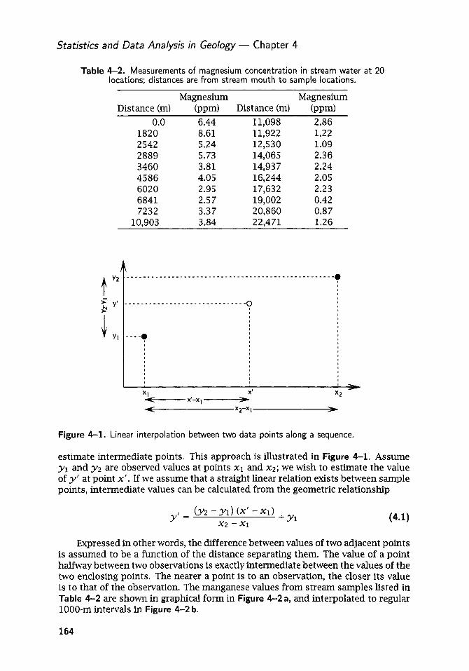
Statistics and Data Analysis in Geology - Chapter 4
Table 4-2. Measurements of magnesium concentration in stream water at 20 locations; distances are from stream mouth to sample locations.
Magnesium Magnesium Distance (m) (ppm) Distance (m) (ppm)
0.0 6.44 11,098 2.86 1820 8.61 2542 5.24 2889 5.73 3460 3.81 4586 4.05 6020 2.95 684 1 2.57 7232 3.37
10,903 3.84
11,922 12,530 14,065 14,937 16,244 17,632 19,002 20,860 22,471
1.22 1.09 2.36 2.24 2.05 2.23 0.42 0.87 1.26
Figure 4-1. Linear interpolation between two data points along a sequence.
estimate intermediate points. This approach is illustrated in Figure 4-1. Assume y1 and y2 are observed values at points X I and x2; we wish to estimate the value of y' at point x' . If we assume that a straight linear relation exists between sample points, intermediate values can be calculated from the geometric relationship
Expressed in other words, the difference betweenvalues of two adjacent points is assumed to be a function of the distance separating them. The value of a point halfway between two observations is exactly intermediate between the values of the two enclosing points. The nearer a point is to an observation, the closer its value is to that of the observation. The manganese values from stream samples listed in Table 4-2 are shown in graphical form in Figure 4-2 a, and interpolated to regular 1000-m intervals in Figure 4-2 b.
164

l o ] 8
0
Analysis of Sequences of Data
0 . 0 . a I ~ , I J I ~ I I I I ~ I I I J ~ I I I l
0
10-
8-
5 n - 6-’
z 4-
2-
0
d 2 4 ‘I
0 0
0
0 0 0 0 0 0 0 0
o o o o o 0 0 o o o o o b
I I I I I I I 0 I I I I I I I I I I I I I l l I
2 4
0 a
0 . 0
0 @ O
Distance, m
Figure 4-2. Magnesium concentration (parts per million) in water at 20 stream locations, measured in meters from stream mouth. ( a ) Original field measurements. (b) Values interpolated a t 1000-m intervals.
Although linear interpolation is simple, it possesses certain drawbacks in many applications. If the number of equally spaced points is approximately the same as the number of original points, and the original points are somewhat uniformly spaced, the technique will give satisfactory results. However, if there are many more original points than interpolated points, most of the original data will be ig- nored because only two surrounding points determine an interpolated value. If the original data possess a large random component which causes values to fluctuate widely, interpolated points may also fluctuate unacceptably. Both of these objec- tions may be met by techniques that consider more than two of the original values, perhaps by fitting a linear function that extends over several adjacent values. Wilkes (1966) devotes an entire chapter to various interpolation procedures.
If the original data are sparse and several values must be estimated between each pair of observations, linear interpolation will perform adequately, provided the idea of uniformity of slope between points is reasonable. In any problem where points are interpolated between observations, however, you must always remember that you cannot create data by estimation using any method. The validity of your result is controlled by the density of the original values and no amount of interpo- lation will allow refinement of the analysis beyond the limitations of the data. For example, we could estimate the magnesium content of the river at 500-m intervals, or even at every 5 m, but it is obvious that these new values would provide no additional information on the distribution of the metal in the stream.
We will next consider a method that produces equally spaced estimates of a variable and considers all observations between successive points of estimation.
165

Statistics and Data Analysis in Geology - Chapter 4
Figure 4-3. (a) Data sequence considered as a step function or "rectangular curve." ( b ) Equally spaced sequence created by rectangular integration. Shaded intervals in (a) and (b ) have the same areas.
The technique is called rectangular integration. If we regard the original data as a rectangular curve or step function in which the interval from one observation to the succeeding observation has a constant value, a data set might have the form shown in Figure 4-3 a. If we wish to create an equally spaced approximation to this distri- bution, we can generate another step function of rectangles of equal length whose areas equal the total areas of the original rectangles. This is shown graphically in Figure 4-3 b, with the resulting sequence of equally spaced values derived from the data in part a. The shaded area under the curve is the same in both illustrations. This procedure has the advantage of considering all data within an interval in es- timating a point. Also, because the area under the estimated curve is equal to the area under the original curve, observations used in the estimation of a point are weighted proportionally to the length of interval they represent.
Calculation of an estimate by rectangular integration is easy in theory but presents a somewhat difficult programming challenge. Starting at one estimated point, the distance to the next observation must be calculated, multiplied by the magnitude of the observation to give the rectangular area, and the process repeated through all successive observations up to the next estimated point. That point is determined by summing the areas just found and dividing by the equally spaced interval to give the estimated value. The initial estimated point in a sequence is taken as the same as the first preceding data point.
An obvious difference in the two interpolation procedures is apparent when original data are sparse and more than one point must be estimated between two ob- servations. Using linear interpolation, values will be created which lie on a straight line between two surrounding data points. In contrast, rectangular integration will create estimates that are equal to the first observation.
In the study of a metamorphic halo around an intrusive, a diamond-drill core was taken perpendicular to the intrusive wall. The entire core was split and all gar- net crystals exposed on the split surface were removed, individually crushed, and
166

Analysis of Sequences of Data
1 5 -
10
2 5 301
0
b
( I r r I 4 4 I I 1 I I 1 8 8 I I 1 8 1 I I I I I 1 0 0 4 1 1 I t 1 I f I I r 1 1 8 I I I I 4 I 0 1 ) I I 8 I O U I ! 1
0 0
0
0
0 .
0 0
0 0
0 0
0
a
10 I I I I I I I I I I I I I 1 1 ' ' 1 ' ' 1 ' " ' 1 ' " ' 1 ' " ' " " ' I ' ' " " ' " I " " ' " " I 0 100 200 300 400 5 0 0 600
2 5 301 Y 2ol
0 0 0 0
0 0
0 0 0 0
0
analyzed for iron content by a rapid spectrochemical method. Both the spacing between successive crystals and their iron content fluctuate through a wide range. Data from this core are shown in Figure 4-4a and are given in file GARNETS.TXT. A generalized picture of compositional changes is desired, but the data seem too erratic for direct interpretation. As a preparatory step to further analysis, the data may be approximated by equally spaced estimates. The desired interval is 50 cm. Here we are presented with a situation that is different from the river data; obser- vations are more abundant than estimates and we wish to preserve as much of the original information as possible. Rectangular integration seems more appropriate in this instance than linear interpolation. Figure 4-4 b shows .the result of inter- polating iron concentration to 50-cm intervals by rectangular integration. It may be instructive to compare these results with those from linear interpolation and to compare both with the overlying original data to see how much detail is lost by the two approximation processes.
In geology, equal spacing procedures have been most widely used to pretreat stratigraphic data (measured sections, drilling-time logs, and similar records) prior to filtering or time-trend analysis. Time-series methods, such as autocorrelation and spectral analysis, require equally spaced data. Time-series techniques are in- herently more powerful than other analytical methods for examining sequential data, and their use has become widespread. However, they require long strings of data, which has restricted their application to geophysics, well-log analysis, and
167

Statistics and Data Analysis in Geology - Chapter 4
the study of stratigraphic sequences and diamond-drill cores through ore deposits. Some work also has been done on mineral successions along traverses across thin sections. These applications will be considered in greater detail later in this chapter.
Markov Chains In many geologic investigations, data sequences may be created that consist of ordered successions of mutually exclusive states. An example is a point-count tra- verse across a thin section, where the states are the minerals noted at succeeding points. Measured stratigraphic sections also have the form of series of lithologies, as may drill holes through zoned ore bodies where the rocks encountered are clas- sified into different types of ore and gangue. Observations along a traverse may be taken at equally spaced intervals, as in point counting, or they may be taken wherever a change in state occurs, as is commonly done in the measurement of stratigraphic sections. In the first instance, we would expect runs of the same state; that is, several successive observations could conceivably fall in the same category. This obviously cannot happen if observations are taken only where states change.
Table 4-3. Stratigraphic succession shown in Figure 4-4 coded into four mutually exclusive states of sandstone (A) , limestone ( B ) , shale ( C ) ,
and coal ( D ) ; observations taken a t 1-ft intervals.
TOP C C B C A C C B C A C C B C A A A B C C A A B A C A C C A D A C C A C A D C A C A D B A D C C B C D c c c c c
A A A A A A C Bottom
Sometimes we are interested in the nature of transitions from one state to another, rather than in the relative positions of states in the sequence. We can employ techniques that sacrifice all information about the position of observations within the succession, but that provide in return information on the tendency of one state to follow another. The data in Table 4-3 represent the stratigraphic section shown in Figure 4-5, in which the sedimentary rock has been classified at successive points spaced 1 ft apart. The lithologies include four mutually exclusive states-sandstone, limestone, shale, and coal, arbitrarily designated A, B, C , and D , respectively. A 4 x 4 matrix can be constructed, showing the number of times a given rock type is succeeded, or overlain, by another. A matrix of this type is called a transition frequency matrix and is shown below. The measured stratigraphic section contains 63 observations, so there are (n - 1) = 62 transitions. The matrix is read “from rows to columns,” meaning, for example, that a transition from state
168

Analysis of Sequences of Data
from C
Figure 4-5. Measured stratigraphic column in which lithologies have been classified into four mutually exclusive states of sandstone (a), limestone (b), shale (c), and coal ( d ) .
B 0 5 z o i 5 2 18 3 28
A to state C is counted as an entry in element a1,3 of the matrix. That is, if we read from the row labeled A to the column labeled C , we see that we move from state A into state C five times in the sequence. Similarly, there are five transitions from state C to state A in the sequence; this number appears as the matrix element defined by row C and column A. The transition frequency matrix is a concise way of expressing the incidence of one state following another:
Row Totals to
A B C D A r18 0 5 01 23
D L 0 0 3 21 5 Column Totals 23 7 28 5 63 Grand Total
Note that the row totals and the column totals wil l be the same, provided the section begins and ends with the same state; otherwise two rows and columns will differ by one. Also note that, unlike most matrices we have calculated before, the transition frequency matrix is asymmetric and in general ai,j # aj,i.
The tendency for one state to succeed another can be emphasized in the matrix by converting the frequencies to decimal fractions or percentages. If each element in the i t h row is divided by the total of the i t h row, the resulting fractions express the relative number of times state i is succeeded by the other states. In a probabilistic sense, these are estimates of the conditional probability, p (jli), the probability
169

Statistics and Data Analysis in Geology - Chapter 4
that state j will be the next state to occur, given that the present state is i. [We here introduce the unconventional but equivalent notation, p ( i - j ) , which can be read as the probability that state i will be followed by state j. This alternative notation will be useful later.]
A B C D
from
to A B C D
0.78 0 0.22 0 0 0.71 0.29 0 0.18 0.07 0.64 0.11 0 0 0.60 0.40
Row Totals
1 .oo 1 .oo 1.00 1 .oo
Here, for example, we see that if we are in state C at one point, the probability is 64% that the lithology 1 ft up will also be state C. The probability is 18% that the lithology will be state A, 7% that it will be state B, and 11% that it will be state D. Since the four states are mutually exclusive and exhaustive, the lithology must be one of the four and so their sum, given as the row total, is 100%.
If we divide the row totals of the transition frequency matrix by the total num- ber of transitions, we obtain the relative proportions of the four lithologies that are present in the section. This is called the marginal (or fixed) probability vector:
C 0.44 D F1 0.08
You will recall from Chapter 2 (Eq. 2.7) that the joint probability of two events, A and B , is
p ( A , B ) = p ( B I A ) p ( A )
rearranging ,
So, the probability that state B will follow, or overlie, state A is the probability that both state A and B occur, divided by the probability that state A occurs. If the occurrence of states A and B are independent, or unconditional,
and
That is, the probability that state B will follow state A is simply the probability that state B occurs in the section, which is given by the appropriate element in the fixed probability vector. If the occurrences of all the states in the section are independent, the same relationship holds for all possible transitions; so, for example,
This allows us to predict what the transition probability matrix should look like if the occurrence of a lithologic state at one point in the stratigraphic interval were
170

Analysis of Sequences of Data
completely independent of the lithology at the immediately underlying point. The expected transition probability matrix would consist of rows that were all identical to the fixed probability vector. For our stratigraphic example, this would appear as
A B C D
from
to A B C D
0.37 0.11 0.44 0.08 0.37 0.11 0.44 0.08 0.37 0.11 0.44 0.08 0.37 0.11 0.44 0.08
Row Totals
1.00 1 .oo 1 .oo 1 .oo
We can compare this expected transition probability matrix to the transition proba- bility matrix we actually observe to test the hypothesis that all lithologic states are independent of the immediately preceding states. This is done using a x 2 test, first converting the probabilities to expected numbers of occurrences by multiplying each row by the corresponding total number of occurrences:
Expected Frequencies Expected Transition Probabilities
0.37 0.11 0.44 0.08 0.37 0.11 0.44 0.08
0.37 0.11 0.44 0.08 0.37 0.11 0.44 0.08
Totals
x 23= x 7 = x 28= x 5 =
8.5 2.5 10.1 1.8 2.6 0.8 3.1 0.6
10.4 3.1 12.3 2.2 1.9 0.6 2.2 0.4
The x2 test is similar in form to the test equation (Eq. 2.65) described in Chapter 2. Each element in the transition frequency matrix constitutes a category, with both an observed and an expected number of transitions. These are compared by
(0 - E)' x2=c c I;
where 0 is the observed number of transitions from one state to another, and E is the number of transitions expected if the successive states are independent. The test has (m - 1)' degrees of freedom, where m is the number of states (a degree of freedom is lost from each row because the probabilities in the rows sum to 1.00). As with other types of x 2 tests, each category must have an expected frequency of at least five transitions. This is not the case in this example, but we can still make a conservative test of independence by calculating the test statistic using the four categories whose expected frequency is greater than five. The remaining categories can be combined until their expected frequencies exceed five.
The categories include the transitions A - A, A - C, C - A, and C - C. Combined categories can be formed of all elements in the B row, all elements in the D row, and the combination of transitions A - B , A - D, C - B and C - D. The resulting x2 statistic is
2 - (18 - 8.5)' + ( 5 - 10.4)' + (5 - 10.1)' + (18 - 12.3)' - 8.5 10.4 10.1 12.3
+ 7.0 5.0 9.8 (7 - 7.0)' + (5 - 5.0)' + ( 5 - 9.8)'
= 20.99
171

Statistics and Data Analysis in Geology - Chapter 4
The critical value of x2 for nine degrees of freedom and a 5% level of significance is 16.92; the test value comfortably exceeds this, so we may conclude that the hy- pothesis of independence of successive states is not correct. There is a statistically significant tendency for certain states to be preferentially followed by certain other states.
A sequence in which the state at one point is partially dependent, in a prob- abilistic sense, on the preceding state is called a Markov chain (named after the Russian statistician, A.A. Markov). A sequence having the Markov property is inter- mediate between deterministic sequences and completely random sequences. Our stratigraphic section exhibits first-order Markov properties; that is, the statistical dependency exists between points and their immediate predecessors. Higher order Markov properties can exist as well. For example, a second-order Markov sequence exhibits a significant conditional relationship between points that are two steps apart.
From the transition probability matrix we can estimate what the lithology will be 2 ft (that is, two observations) above a given point. Suppose we start in limestone (state B) . The following probabilities estimate the lithology to be encountered at the next point upward:
State A (sandstone) 0% State B (limestone) 71% State C (shale) 2 9% State D (coal) 0%
Suppose the next point actually falls in a shale; we can then determine the probable lithology of the following point:
State A (sandstone) 18% State B (limestone) 7% State C (shale) 64% State D (coal) 11%
So, the probability that the lithologic sequence will be limestone -* shale - limestone is
However, there is another way to reach the limestone state in two steps. The se- quence limestone - limestone - limestone is also possible. The probability attached to this sequence is
p ( B - C ) x p ( C - B ) = 29% x 7% = 2%
p ( B -, B ) X p ( B + B ) = 7 1 % ~ 71%= 50%
Since the other transitions limestone - sandstone and limestone - coal have zero probability, these two sequences are the only possible ones which lead from limestone and back again in two steps. The probability that the lithology two steps above a limestone will also be a limestone, regardless of the intervening lithology, is the sum of all possibilities. That is,
p ( B - A - B ) = 0% p ( B - B - B ) = 50%
p ( B - D - B ) = 0% Total = 52%
p ( B - C - B ) = 2%
172

Analysis of Sequences of Data
The same reasoning can be applied to determine the probability of any lithology two steps hence, from any starting lithology. However, all of the various sequences do not have to be worked out individually, because the process of multiplying and summing is exactly that used for matrix multiplication. If the transition probability matrix is multiplied by itself (that is, the matrix is squared), the result is the second- order transition probability matrix describing the second-order Markov properties of the succession:
1 0.78 0 0.22 0 0.64 0.02 0.31 0.02 0 0.71 0.29 0 1' = [ 0.05 0.52 0.39 0.03
0.18 0.07 0.64 0.11 0.26 0.09 0.54 0.11 0 0 0.60 0.40 0.11 0.04 0.62 0.23
Note that the rows of the squared matrix also sum to 100%. The existence of a significant second-order property can be checked in exactly
the same manner as we checked for independence between successive states, by using a x2 test. If you repeat the test performed earlier, but using the second-order transition probability matrix, you should find that the sequence has no significant second-order properties.
We can estimate the probable state to be encountered at any step in the future simply by powering the transition probability matrix the appropriate number of times. If the matrix is raised to a sufficiently high power, it reaches a stable state in which the rows all become equal to the fixed probability vector, or in other words, becomes an independent transition probability matrix and will not change with additional powering.
You will note in the example that the highest transition probabilities are from one state to itself, particularly from sandstone to sandstone, from limestone to limestone, and from shale to shale. It is obvious that these transition probabili- ties are related to the thicknesses of the stratigraphic units being sampled and the distance between the sample points. For example, the frequencies along the main diagonal of the transition frequency matrix would be doubled while off-diagonal frequencies remained unchanged if observations were made every half-foot. This would greatly enhance the Markovian property, but in a specious manner. Select- ing the appropriate distance between sampling points can be a vexing problem; if observations are too closely spaced, the transition matrix reflects mainly the thick- ness of the more massive stratigraphic units. If the spacing is too great, thin units may be entirely missed.
Embedded Markov chains The difficulty of selecting an appropriate sampling interval can be avoided if ob- servations are taken only when there is a change in state. A stratigraphic section, for example, would be recorded as a succession of beds, each one of a different lithology than the immediately preceding bed. Table 4-4 contains the record of successive rock types penetrated by a well drilled in the Midland Valley of Scotland (these data are contained in file MIDLAND.TXT). The well was drilled through 1600 ft of Coal Measures of Carboniferous age, consisting of interbedded shales, silt- stones, sandstones, and coal beds or root zones. These sediments are interpreted as having been deposited in a delta plain environment subject to repeated flooding, so we would expect that certain lithologies would occur in preferred relations to
173

Statistics and Data Analysis in Geology - Chapter 4
A - 0 13 36 19 5 2 - B 2 9 0 5 4 O
D 29 1 44 0 3 E 26 23 9 9 0
from c 35 2 0 45 12
Table 4-4. Successive lithologic states encountered in a drill hole through the Coal Measures in the Midland Valley of Scotland (after Doveton,
1971); mutually exclusive states are barren shale ( A ) , shale with fossils of nonmarine bivalves ( B ) , siltstone ( C ) , sandstone (D), and coal or
root zone ( E ) ; read across rows. Data are in file MIDLAND.TXT.
120 38 94 77 67
TOP - B E A E A D A C D C D C A B E A D C D C D C A E D C A D C A E C D C B E A D C D C D C A B A E D C A E C A D E A D A C A B E A D C A E C D C A B A E A D E A D C E A C D C D C D C A B E A B A B A B E A B A C A C A B A B E A C D C D C D C A C B E A C A C B E C A D C A C D C E A C D A C D C B A B E A C D C A B A B E A D A C E A D A D C A E A C D A E A E A C D C E C A B C E C A D B E A D C D E A D A C A B E A B A B E A B A B E C A C D A E A C D C D C A C A C E A C D C D C A B E A D E A C D C D E C D C E A C A E A C A E A C A B C D A E A C D C E A C B E A C A E A D A B E A C D E A D C A B E A D C D E A D C D A E A C D C A D A E A D A D C A C E D A B D B A E A C A E C D C D C D A E A E C D A B E A B E A E A C D E A D A D E C D C A E A E A C D A E C D B E A D C D C A D A B A B E A D B A E A - Bottom
others. The data are taken from one of a large number of wells studied by Doveton (1971).
The four-state transition frequency matrix for the section in the Scottish well is given below. One obvious difference between this matrix and the one we have considered previously is that all the diagonal terms must be zero, since a state cannot succeed itself. The transition probability matrix, computed by dividing each element of the transition frequency matrix by the appropriate row total, shares this same characteristic. Sequences in which transitions from a state to itself are not permitted are called embedded Mavkov chains, and their analysis presents special problems that have not always been appreciated by geologists studying
to stratigraphic records. A B C D E Z Z s
The lithologic states have been coded as (A) unfossiliferous shale and mudstone, ( B ) shales containing nonmarine bivalves, (C) siltstone, (D) sandstone, and ( E ) coals and root zones. The corresponding transition probability matrix is
174
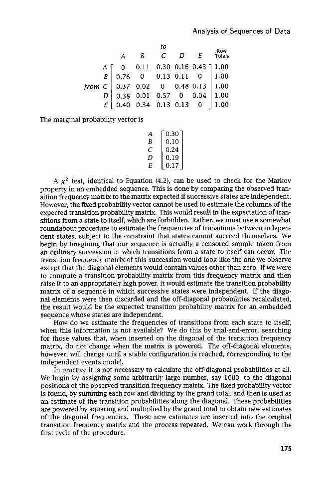
Analysis of Sequences of Data
0.43 - 0
0.13 0.04
0
1.00 1.00 1.00 1.00 1.00
A B
from C D E
The marginal probability vector is
A 0.30
D C [E] 0.19
E 0.17
A x 2 test, identical to Equation (4.2), can be used to check for the Markov property in an embedded sequence. This is done by comparing the observed tran- sition frequency matrix to the matrix expected if successive states are independent. However, the fixed probability vector cannot be used to estimate the columns of the expected transition probability matrix. This would result in the expectation of tran- sitions from a state to itself, which are forbidden. Rather, we must use a somewhat roundabout procedure to estimate the frequencies of transitions between indepen- dent states, subject to the constraint that states cannot succeed themselves. We begin by imagining that our sequence is actually a censored sample taken from an ordinary succession in which transitions from a state to itself can occur. The transition frequency matrix of this succession would look like the one we observe except that the diagonal elements would contain values other than zero. If we were to compute a transition probability matrix from this frequency matrix and then raise it to an appropriately high power, it would estimate the transition probability matrix of a sequence in which successive states were independent. If the diago- nal elements were then discarded and the off-diagonal probabilities recalculated, the result would be the expected transition probability matrix for an embedded sequence whose states are independent.
How do we estimate the frequencies of transitions from each state to itself, when this information is not available? We do this by trial-and-error, searching for those values that, when inserted on the diagonal of the transition frequency matrix, do not change when the matrix is powered. The off-diagonal elements, however, will change until a stable configuration is reached, corresponding to the independent events model.
In practice it is not necessary to calculate the off-diagonal probabilities at all. We begin by assigning some arbitrarily large number, say 1000, to the diagonal positions of the observed transition frequency matrix. The fixed probability vector is found, by summing each row and dividing by the grand total, and then is used as an estimate of the transition probabilities along the diagonal. These probabilities are powered by squaring and multiplied by the grand total to obtain new estimates of the diagonal frequencies. These new estimates are inserted into the original transition frequency matrix and the process repeated. We can work through the first cycle of the procedure.
- 0 0.11 0.30 0.16 0.76 0 0.13 0.11 0.37 0.02 0 0.48 0.38 0.01 0.57 0
- 0.40 0.34 0.13 0.13
175

Statistics and Data Analysis in Geology - Chapter 4
A - B
from c D E -
Step 1. Initial estimate of transition frequency matrix, with 1000 inserted in each diagonal position.
1000 13 36 19 52 29 1000 5 4 0 3 5 2 1000 45 12 29 1 44 1000 3 26 23 9 9 1000
- 0.208
0.192 0.203
0.200 0.198 -
1120 1038 1094 1077 1067 5397 Grand Total
0.208 0.192 0.203 0.200 0.198
Step 2. Estimate of transition probabilities of diagonal elements, found by dividing row totals by grand total.
Row A B C D E Totals
to
A B
from C D E
Step 3. Square the probabilities along the diagonal. Step 4. Second estimate of transition frequency matrix using new diagonal
elements calculated by multiplying probabilities on the diagonal by the grand total of 5397. Off-diagonal terms are the original observed frequencies. New row totals and grand total are then found
A B
from C D E
to A B C D E
232 13 36 19 52 29 199 5 4 0 3 5 2 222 45 12 29 1 44 215 3
- 26 23 9 9 2 1 1
Row Totals
352 237 316 292 278
1475 Grand Total
The process is repeated again and again, until the estimated transition frequen- cies along the diagonal do not change from time to time. This generally requires about 10 to 20 iterations, depending upon how closely the initial guesses were to the final, stable estimates. In this example, the estimates do not change after 10 iterations.
The final form of the transition frequency matrix with estimated diagonal fre- quencies is given below.
176

Analysis of Sequences of Data
- A 0.125 0.026 0.083 0.064 0.055 B 0.026 0.006 0.017 0.013 0.012
from C 0.083 0.017 0.055 0.043 0.036 D 0.064 0.013 0.043 0.033 0.028 E - 0.055 0.012 0.036 0.028 0.024 -
A B
from C D E
Column Totals
A B
from C D E
A B 66 13 29 3 35 2 29 1 26 23 185 42
- - 65.5 13.6 43.5 33.5 28.8 13.6 3.1 8.9 6.8 6.3 43.5 8.9 28.8 22.5 18.9 33.5 6.8 22.5 17.3 14.7
- 28.8 6.3 18.9 14.7 12.6 -
to C D E
36 19 52 5 4 0
29 45 12 44 17 3 9 9 12
123 94 79
Row Totals
186 41 123 94 79
5 23 Grand Total
177

Statistics and Data Analysis in Geology - Chapter 4
Note that the matrix is symmetrical and the diagonal elements remain unchanged, within the limits of rounding error. The off-diagonal elements are the expected frequencies of transitions within the embedded sequence, assuming independence between successive states. If the diagonal elements are stripped from the matrix, it may be compared directly to the observed transition frequency matrix because the row and column totals of the two are the same, again within rounding limits.
The comparison by x 2 methods yields a test statistic of x 2 = 172. The test has v = (m - 1)2 - m degrees of freedom, where m is the number of states, or in this example, v = 11. The critical value of x 2 for 11 degrees of freedom and an o( = 0.05 level of significance is 19.68, which is far exceeded by the test statistic. Therefore, we must conclude that successive lithologies encountered in the Scottish well are not independent, but rather exhibit a strong first-order Markovian property.
If tests determine that a sequence exhibits partial dependence between succes- sive states, the structure of this dependence may be investigated further. Simple graphs of the most significant transitions may reveal repetitive patterns in the suc- cession. Modified x 2 procedures are available to test the significance of individual transition pairs. Some authors have found that the eigenvalues extracted from the transition probability matrix are useful indicators of cyclicity. (It should be noted, however, that extracting the eigenvectors from an asymmetric matrix such as the transition probability matrix may not be an easy task!) These topics will not be pursued further in this book; the interested reader should refer to the texts by Ke- meny (1983) and Norris (1997), as well as the book on quantitative sedimentology by Schwarzacher (1975). Chi-square tests appropriate for embedded sequences are discussed by Goodman (1968). In a geological context, the articles by Dove- ton (1971) and Doveton and Skipper (1974), plus the comment by Tiirk (1979), are recommended.
Series of Events An interesting type of time series we will now consider is called a series of events. Geological examples of this type of data sequence include the historical record of earthquake occurrences in California, the record of volcanic eruptions in the Mediterranean area, and the incidence of landslides in the Tetons. The character- istics of these series are (a) the events are distinguishable by when they occur in time; (b) the events are essentially instantaneous; and (c) the events are so infre- quent that no two occur in the same time interval. A series of events is therefore nothing more than a sequence of the intervals between occurrences. Our data may consist of the duration between successive events, or the cumulative length of time over which the events occur. One form may be directly transformed into the other.
Series-of-events models may be appropriate for certain types of spatially dis- tributed data. We might, for example, be interested in the occurrence of a rare mineral encountered sporadically on a traverse across a thin section or in the ap- pearance of bentonite beds in a vertical succession of sedimentary rocks. Justifica- tion for applying series-of-events models to spatial data may be tenuous, however, and depends on the assumption that the spatial sequence has been created at a constant rate. This assumption probably is reasonable in the first example, but the second requires that we assume that the sedimentation rate remained constant through the series.
The historic record of eruptions of the volcano Aso in Kyushu, Japan, has been kept since 1229 (Kuno, 1962), and is given in Table 4-5 and file ASO.TXT. Aso is
178

Analysis of Sequences of Data
Table 4-5. Years of eruptions of the volcano Aso for the period 1229-1962.
1229 1239 1240 1265 1269 1270 1272 1273 1274 1281 1286 1305 1324 1331 1335 1340 1346 1369 1375
1376 1377 1387 1388 1434 1438 1473 1485 1505 1506 1522 1533 1542 1558 1562 1563 1564 1576 1582
1583 1584 1587 1598 1611 1612 1613 1620 1631 1637 1649 1668 1675 1683 1691 1708 1709 1765 1772
1780 1804 1806 1814 1815 1826 1827 1828 1829 1830 1854 1872 1874 1884 1894 1897 1906 1916 1920
1927 1928 1929 1931 1932 1933 1934 1935 1938 1949 1950 1951 1953 1954 1955 1956 1957 1958 1962
a complex stratovolcano, but all historic eruptions have been explosive, ejecting ash of andesitic composition. Although the ancient monastic records contain an indication of the relative violence and duration of some eruptions, for all practical purposes we must regard the record as one of indistinguishable instantaneous ex- plosive events. Analysis of volcanic histories may shed some light on the nature of eruptive mechanisms and can even lead to physical models of the structure of volcanoes (Wickman, 1966). Of course, we would also hope that such studies might lead to predictive tools to forecast future eruptions.
Studies of series of events may have several objectives. Usually, an investigator is interested in the mean rate of occurrence, or number of events per interval of time. In addition, it may be necessary to examine the series in more detail, in order to estimate any pattern that may exist in the events. This additional information can be used to determine the precision of the estimate of the rate of occurrence, to assess the appropriateness of the sampling scheme, to detect a trend, and to detect other systematic features of the series.
Because series of events are very simple, in the sense that they consist of nom- inal occurrences (presence-absence), simple analytical techniques may prove to be the most effective. Cox and Lewis (1966) described a variety of graphical tools that are useful in examining series of events. These are illustrated using the data on the eruptions of Aso from Table 4-5.
A cumulative plot of the total number of events (nt) to have occurred at or before time t , against time t , is given in Figure 4-6. This plot is especially good for showing changes in the average rate of occurrence. The slope of a straight line connecting any two points on the cumulative plot is the average number of events per unit of time for the interval between the two points.
179

Statistics and Data Analysis in Geology - Chapter 4
100
80
60 L u- L 0
QJ n 5 40 z
20
0 1200 1400 1600 1800 2 30
Year of event
Figure 4-6. Cumulative number of eruptions of the Japanese volcano Aso plotted against years of eruptions.
Figure 4-7. Histogram of number of eruptions of the Japanese volcano Aso occurring in successive 100-yr intervals.
A histogram of the number of events occurring in successive equal intervals of time is given in Figure 4-7. This histogram directly indicates local periods of fluc- tuation from the average rate of occurrence. The pattern shown by the histogram is sensitive to the length of the chosen intervals, so more than one histogram may be useful in examining a series.
The empirical survivor function is obtained by plotting the percent “survi- vors,” or Y = proportion of time intervals longer than X, against X = length of time
180

Analysis of Sequences of Data
100 - 70 -
% 30-
Y? 20- 8 '5 s 7:
v, 101 4-
8 5 - 4 - 3 -
2 -
interval. The function estimates the probability that an event has not occurred before time X . In Figure 4-8, the points represent the percentage of intervals be- tween eruptions which are longer than the specified number of years. If events occur randomly in time, the survivor function will be exponential in form.
-0
\ 0
% 0
0
O O 0 0
0
0
D Length of interval, years
Figure 4-8. Empirical survivor function for the Japanese volcano Aso. The vertical axis gives the percent of intervals between eruptions tha t are longer than a specified duration, versus the duration in years along the horizontal axis.
This same function can be plotted in logarithmic form, as log Y against X . The log empirical survivor function is especially good for showing departures from randomness, which appear as deviations from the straight-line form of the plot (Fig. 4-9).
1 n 0 10 20 30 40 50
Length of interval, years D
Figure 4-9. Log empirical survivor function of the Japanese volcano Aso. The vertical axis of Figure 4-8 is expressed in logarithmic form.
181

Statistics and Data Analysis in Geology - Chapter 4
10
0 0 10 20 30 40 50 0
t i + l - t i i n years
Figure 4-10. Serial correlation of durations between successive eruptions of the Japanese volcano Aso. Vertical axis is duration of quiet before the i th eruption, and horizontal axis is duration after the zth eruption.
A scatter diagram of the serial correlation, or first-order autocorrelation, of successive intervals between events is shown in Figure 4-10. The degree of cor- respondence between the length of an interval and the length of the immediately preceding interval is shown by plotting xi = ti+l - t i against yi = ti - t i -1 where ti is the time of occurrence of the i t h event. This plot reveals any tendency for intervals to be followed by intervals of similar length. A scatter diagram with large dispersion and relatively high concentrations of points near the axes is typical of random series of events.
In most series-of-events studies, we hope that we can describe the basic fea- tures of the series in a way that will suggest a physical mechanism for the lengths of the intervals between occurrences. First we must consider the possibility of a trend in the data. We may check for a trend in two ways. A series may be subdivided into segments of equal length, provided each segment contains several observations. The numbers of events within each segment are taken to be observations located at the midpoints of the segments. A regression can then be run with these numbers as the dependent variable, yi, and the locations of the midpoints of the segments as values of Xi. The slope coefficient of the regression can be tested by the ANOVA given later in Table 4-9 (p. 197) to determine if it is significantly different from zero. The process is illustrated in Figure 4-11. Unfortunately, this test is not par- ticularly efficient because degrees of freedom are lost when the series is divided into segments.
There are tests specifically designed to detect a trend in the rate of occurrence of events by comparing the midpoint of the sequence to its centroid. If the sequence is relatively uniform, the two will be very similar, but if there is a trend the centroid will be displaced in the direction of increasing rate of occurrence. If t i is the time or distance from the start of the series to the i t h event and N is the total number of events, we can calculate the centroid, S , by
182

Analysis of Sequences of Data
5 2 5 Y ; 20- L 0) n 2 1 5 -
o. 2 10-
0 .- Y
01 L
n k 5-
5 2 0
0
0
0 0
This statistic can in turn be used in Equation (4.4),
S - 1/2T Z =
T / r n (4.4)
where T is the total length of the series, z is the standardized normal variate, and the significance of the test result can be determined by normal tables such as Appendix Table A. 1.
The test is very sensitive to changes in the rate of occurrence of events. Specif- ically, if the events are considered to be the result of a process
yt = p + B t (4.5)
the null hypothesis states that f i = 0. You will recognize that the model is expo- nential; if f i has any value other than zero, the rate of occurrence of Yt will change with t. It is this possibility that we are testing.
If no trends are detected in the rate of occurrence, we may conclude that the series of events is stationary. We can next check to see if successive occurrences are independent. This can be done by computing the autocorrelation of the lengths between events. That is, we regard the intervals between events as a variable, X , located at equally spaced points. If the intervals are not independent, this will be expressed as a positive autocorrelation with a tendency for large values of Xi (long intervals between events) to be succeeded by large values; similarly, there will be a tendency for small values of xi (short intervals) to be followed by other smallvalues. We can compute autocorrelation coefficients for successive lags and test these for significance. Usually only the first few lags will be of interest. If the autocorrelation coefficients are not significantly different from zero, as tested by methods that will
183

Statistics and Data Analysis in Geology - Chapter 4
be developed later in this chapter, we can conclude that the events are occurring independently in time or space.
If we have established that the series is neither autocorrelated nor contains a trend, we may wish to test the possibility that the events are distributed accord- ing to a Poisson distribution. You will recall from Chapter 2 that the Poisson is a discrete probability distribution that can be regarded as the limiting case of the binomial when n, the number of trials, becomes very large, and p , the probability of success on any one trial, becomes very small. We can imagine that our time series is subdivided into n intervals of equal duration. If events occur randomly, the number of intervals that contain exactly 0, 1, 2 , . . . , x events will follow the bi- nomial distribution. As we make the lengths of the intervals progressively shorter, n becomes progressively larger and the probabilities of occurrence decline. The binomial distribution becomes difficult to compute, but the Poisson can be readily used because it does not require either n or p directly. Instead, the product np = h is all that is needed, which is given by the rate of occurrence of events.
The Poisson probability model assumes that (a) the events occur independently, (b) the probability that an event occurs does not change with time, (c) the proba- bility that an event will occur in an interval is proportional to the length of the interval, and (d) the probability of more than one event occurring at the same time is vanishingly small.
The equation for the Poisson distribution in this instance is
p ( X ) = e - ” A X / X ! (4.6)
Note that the rate of occurrence, A, is the only parameter of the distribution. Typ- ical Poisson frequency distributions are shown in Figure 4-12. The distribution is applicable to such problems as the rate that telephone calls come to a switchboard or the length of time between failures in a computer system. It seems reasonable that it also may apply to the series of geological events described at the beginning of this section. If we can determine that our series follows a Poisson distribution, we can use the characteristics of the distribution to make probabilistic forecasts of the series.
The Kolmogorov-Smirnov test provides a simple way to test the goodness of fit of a series of events to that expected from a Poisson distribution. First, the series must be converted to a cumulative form
ti yi = - T
where ti is the time from the start of the series to the i t h event, and T is the total length of the series. Three estimates can then be calculated
The first test is simply the maximum positive difference between the observed se- ries and that expected from a Poisson, the second is the maximum negative differ- ence, and the third is the larger of the absolute values of the two. The test statistic,
184

Analysis of Sequences of Data
Figure 4-12. Poisson probability distributions with difFerent rates of occurrence, A , ex- pressed as numbers of occurrences per interval. (a ) h = 6.0. ( b ) h = 2.0. (c) h = 0.6.
D, can be compared to two-tailed critical values given in Appendix Table A.7. If the statistic exceeds the critical value, the maximum deviation is larger than that expected in a sample collected at random from a Poisson distribution.
Runs Tests The simplest type of sequence is a succession of observations arranged in order of occurrence, where the observations are two mutually exclusive categories or states. Consider a rock collector cracking open concretions in a search for fossils. The breaking of a concretion constitutes a trial, and each trial has two mutually exclusive outcomes: The concretion either contains a fossil or it does not. The sequence of successes and failures by the collector during the course of a day forms a special type of time series. We can experimentally create a similar succession by flipping pennies and noting the occurrence of heads or tails. The sequence generated might resemble this set of twenty trials:
H T H H T H T T T H T H T H H T T H H H
We intuitively expect, of course, that about ten heads will appear, and we can de- termine the probability of obtaining this (or any other) number of heads. Here we obtained 11 heads; assuming the coin is unbiased, the probability of obtaining this number in 20 trials is 0.16 or about one in six. We would expect similar trials to contain 9, 10, or 11 heads slightly more than one-third of the time. Results of this experiment follow the binomial distribution, discussed in Chapter 2.
185

Statistics and Data Analysis in Geology - Chapter 4
One aspect that we have not considered, however, is the order in which the heads appear. We probably would regard a sequence such as
H H H H H H H H H H H T T T T T T T T T
as being very strange, although the probability of obtaining this many heads in 20 trials is the same as in the preceding example. At the other extreme, the regular alternation of heads and tails
H T H T H T H T H T H T H T H T H T H H
would also appear very unusual to us, although the probability of the number of heads is unchanged. What arouses our suspicions is not the proportion of heads but the order in which they appear. We assume that heads and tails will occur at random; in the two preceding examples, it seems very unlikely that they have.
We can test these sequences for randomness of occurrence by examining the number of runs. Runs are defined as uninterrupted sequences of the same state. The first set of trials contains 13 runs, the second only 2, and the third contains 19. Runs in the first sequence shown are underlined:
(Start) - H T H H T I J T T T H T I J T H T T H H H 1 1 3 4 5 6 7 8 9 10 11 12 13 (End)
We can calculate the probability that a given sequence of runs was created by the random occurrence of two states (heads and tails, in this example). This is done by enumerating all possible ways of arranging nl items of state 1 and n2 items of state 2. The total number of runs in a sequence is denoted U; tables are available which give critical values of U for specified nl, n2, and level of significance, (x.
However, if nl and n2 each exceed ten, the distribution of U can be closely ap- proximated by a normal distribution, and we can use tables of the standard normal variate z for our statistical tests. The expected mean number of runs in a randomly generated sequence of nl items of state 1 and n2 items of state 2 is
The expected variance in the mean number of runs is
2 2nln2(2nlnZ - nl - n2)
(n1+ n2I2(n1 + n2 - 1) CTU = (4.9)
By these equations, we can determine the mean number of runs and the stan- dard error of the mean number of runs in all possible arrangements of nl and n2 items. Having calculated these, we can create a z-test by Equation (4.10), where U is the observed number of runs:
(4.10)
You will recognize that this is simply Equation (2.37) rewritten to include the runs statistics. We can formulate a variety of statistical hypotheses which can be tested with this statistic. For example, we may wish to see if a sequence contains more
186

Analysis of Sequences of Data
than the expected number of runs from a random arrangement; the null hypothesis and alternative are
H i : U > U
and too many runs leads to rejection. The test is one-tailed. Conversely, we may wish to determine if the sequence contains an improbably low number of runs. The appropriate alternatives are
H o : U r 8 H1: u < u
and too few runs will cause rejection of the null hypothesis. Again, the test is one- tailed. We may wish to reject either form of nonrandomness. A two-tailed test is appropriate, with hypotheses
H o : U = 8 H i : U f 8
We can work through the test procedure for the first series of coin flips and determine the likelihood of achieving this sequence by a random process. The null hypothesis states that there is no difference between the observed number of runs and the mean number of runs from random sequences of the same size. We will use a two-tailed test, and reject if there are too many or too few runs in the sequence. Therefore, the proper alternative is
H i : U f U
Using a 5% (a = 0.05) level of significance, our critical regions are bounded by -1.96 and +1.96. We first calculate the expected mean and standard deviation of runs for random sequences having nl heads (nl = 11) and n2 tails (n2 = 9):
2 11 * 9)(2 * 11 9 - 11 - 9) (9 + 11)*(9 + 11 - 1)
aiJ 2 - ( - = 4.6
The test statistic is = 1.0 U - U 13- 10.9 z=- %
U U 2.1 The number of runs in the sequence is one standard deviation from the mean of all runs possible in such a sequence, and does not fall within the critical region. Therefore, the number of runs does not suggest that the sequence is nonrandom. The other sequences, in contrast, yield very different test results. Because nl and nz are the same for all three sequences, 8 and (TU also are the same. For the second sequence, the test statistic is
2 - 10.9 2.1 z = = -4.2
and for the third, 19 - 10.9
z = = 3.9 2.1
187

Statistics and Data Analysis in Geology - Chapter 4
Both of these values lie within the critical region, and we would reject the hypothesis that they contain the number of runs expected in random sequences.
Geologic applications of this test may not be obvious, because we ordinarily must consider more than two states in a succession. Stratigraphic sections or tra- verses across thin sections, for example, usually include at least three states and these cannot be ranked in a meaningful way. We will consider ways that certain se- quences can be reduced to dichotomous states, but first we will examine a geologic application of the runs test to a traverse through a two-state system.
Simple pegmatites originate by crystallization of the last, volatile-laden sub- stances squeezed off from solidifying granitic magma. Their textures result from simultaneous crystallization of quartz and feldspar at the eutectic point. If the solidifying pegmatite is undisturbed, we might suppose that quartz and feldspar begin to appear at random locations within the cooling body. This situation may persist, with grains crystallizing at random, until the entire mass is solid. However, the presence of one crystal, perhaps feldspar, might stimulate the local crystalliza- tion of additional crystals of feldspar, eventually producing a patchwork texture. Alternatively, growth of a crystal of one state might locally deplete the magma of that constituent, retarding crystallization and resulting in a highly alternating mo- saic of quartz and feldspar. A large slab of polished pegmatite used as a window ledge in the washroom of a geology building provides a way for students to investi- gate these alternative possibilities. The polished surface allows easy discrimination of adjacent grains, so a line drawn on the ledge produces a sequence through the quartz and feldspar grains in the pegmatite. The line on the polished slab may be regarded as a random sample of possible successions through the pegmatite body from which the slab was quarried. The quartz-feldspar sequence along the line is listed in Table 4-6. Our problem is to determine if the alternations between quartz and feldspar form a random pattern; if there is a systematic tendency for one state to succeed itself; or whether there is a tendency for one state to imme- diately succeed the other. Perform a runs test on this data and evaluate the three possibilities.
Table 4-6. Sequence of 100 feldspar (F) and quartz (Q) grains encountered along traverse through pegmatite.
(Start) F Q Q F Q Q F F Q F Q F F F F F F F Q Q F Q F F F Q F F F F Q F F F Q Q F Q F Q Q Q F F F F F Q F F F F F Q Q Q Q F F Q Q Q F F F F F F Q F Q F F F F
F Q F Q F Q F F Q F F F F F Q F F F Q Q F Q F F Q (End)
We will now consider a related statistical procedure for examining what are called runs u p and runs down. We are concerned, not with two distinct states, but whether an observation exceeds or is smaller than the preceding observation. Figure 4-13 shows a typical sequence that can be analyzed by means of a runs test.
The segment abc is a run up, because each observation is larger than the pre- ceding one; similarly, the segment ghi is a run down. Segment cdef is a run down even though the difference between d and e is zero. This is because the interval de lies between segments cd and e f , both of which run downward; therefore, the
188

Analysis of Sequences of Data
X
Figure 4-13. Sequence of data points t o be analyzed by the method of runs up and down.
entire segment cdef can be considered as a single downward run. The interval ij can be considered either as part of the run down g h i or the run up i j k , as the total number of runs remains the same in either case. In this example, we are assuming that the successive points have integer values. If the observations are expressions of magnitude, they ordinarily will contain fractional parts, and ties (two successive points with identical values) are unlikely.
By considering only differences in magnitude between successive points, we have reduced the data sequence to a string having only two states (or three, if ties occur). We can rewrite the sequence in Figure 4-13 in the following form:
+ + + - 0 - + - - o + Regarding the first zero as ‘ I - ” gives a total of five runs, three of “+” and two of
‘ I - ” (it makes no difference in the number of runs if we call the second zero “+” or “-”). We can now apply test procedures outlined for the case of sequences of two dissimilar items (Eqs. 4.8-4.10). We must have a large sample to utilize the normal approximation method presented here, but in most geologic problems, adequate numbers of samples will be available.
Table 4-7. Numbers of radiolarian tests per square centimeter in thin sections of siliceous shale.
(Bottom ofsection) 1 2 3 2 3 5 7 9 9 11 10 12 7 4 3 2 3
2 2 1 0 2 3 2 0 3 3 4 9 1 0 1 0 8 9 1 2 10 12 14 22 17 19 14 4 2 1 0 0 8 14 16 27 (Topof
section)
In the study of a silicified shale unit in the Rocky Mountains, it was noted that the rock contained unusual numbers of well-preserved radiolarian tests. Their presence in the silicified shale suggested a causal relationship, so a sequence of samples was collected at approximately equal intervals in an exposure through the unit. Thin sections were made of the samples and the number of radiolarian tests in a 10 x 10-mm area of the slides was counted. Data for 50 samples are given in Table 4-7 and shown graphically in Figure 4-14. Does the abundance of
189
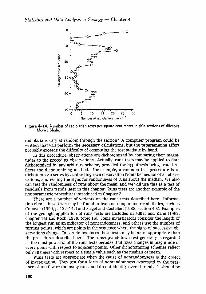
Statistics and Data Analysis in Geology - Chapter 4
10
40
0 5 1 0 1 5 20 25 30 Number of radiolarians per cm2
Figure 4-14. Number of radiolarian tests per square centimeter in thin sections of siliceous Mowry Shale.
radiolarians vary at random through the section? A computer program could be written that will perform the necessary calculations, but the programming effort probably exceeds the difficulty of computing the test statistic by hand.
In this procedure, observations are dichotomized by comparing their magni- tudes to the preceding observations. Actually, runs tests may be applied to data dichotomized by any arbitrary scheme, provided the hypothesis being tested re- flects the dichotomizing method. For example, a common test procedure is to dichotomize a series by subtracting each observation from the median of all obser- vations, and testing the signs for randomness of runs about the median. We also can test the randomness of runs about the mean, and we will use this as a test of residuals from trends later in this chapter. Runs tests are another example of the nonparametric procedures introduced in Chapter 2.
There are a number of variants on the runs tests described here. Informa- tion about these tests may be found in texts on nonparametric statistics, such as Conover (1999, p. 122-142) and Siege1 and Castellan (1988, section 4.5). Examples of the geologic application of runs tests are included in Miller and Kahn (1962, chapter 14) and Rock (1988, topic 16). Some investigators consider the length of the longest run as an indicator of nonrandomness, and others use the number of turning points, which are points in the sequence where the signs of successive ob- servations change. In certain instances these tests may be more appropriate than the procedures described here. The runs-up-and-down test generally is regarded as the most powerful of the runs tests because it utilizes changes in magnitude of every point with respect to adjacent points. Other dichotomizing schemes reflect only changes with respect to a single value such as the median or mean.
Runs tests are appropriate when the cause of nonrandomness is the object of investigation. They test for a form of nonrandomness expressed by the pres- ence of too few or too many runs, and do not identify overall trends. It should be
190

Analysis of Sequences of Data
emphasized that randomness itself cannot be proven, as the condition of random occurrence is implied in the null hypothesis. Rather, at specified levels of signifi- cance, we can demonstrate that the null hypothesis is incorrect and the sequence is therefore not random. Or we can fail to reject the null hypothesis, implying that we have failed to find any indication of nonrandomness. We will next consider proce- dures for detecting trends, or systematic changes in average value, and will find that runs tests may be used to good advantage in conjunction with these procedures.
Least-Squares Methods and Regression Analysis In many types of problems, we are concerned not only with changes along a se- quence, but are also interested in where these changes occur. To examine these problems, we must have a collection of measurements of a variable and also must know the locations of the measurement points. Both the variable and the scale along the sequence must be expressed in units having magnitude: it is not suffi- cient simply to know the order of succession of points. We are interested in the general tendency of the data in most of the examples we will now consider. This tendency will be used to interpolate between data points, extrapolate beyond the data sequence, infer the presence of trends, or estimate characteristics that may be of interest to the geologist. If certain assumptions can justifiably be made about the distribution of the populations from which the samples are collected, statistical tests called regression analyses can be performed.
It must be emphasized that we are now using the expression “sequence” in the broadest possible sense. Regression methods are useful for much more than the analysis of observations arranged in order in time or space; they can be used to analyze any bivariate data set when it is useful to consider one of the variables as a function of the other. It is as though one variable forms a scale along which observations of the other variable are located, and we want to examine the nature of changes in this variable as we move up or down the scale.
Table 4-8. Moisture content of core samples of Recent mud in Louisiana estuary.
Moisture (g water/100 g Depth, ft dried solids)
0.0 5.0
10.0 15.0 20.0 25.0 30.0 35.0
124.0 78.0 54.0 35.0 30.0 21.0 22.0 18.0
The data in Table 4-8 are the moisture contents of samples from a core through Recent marine muds accumulating in a small inlet on the U.S. Gulf Coast in eastern Louisiana. These data are also in file LOUISMUD.TXT. The measurements were made
191
Next Page
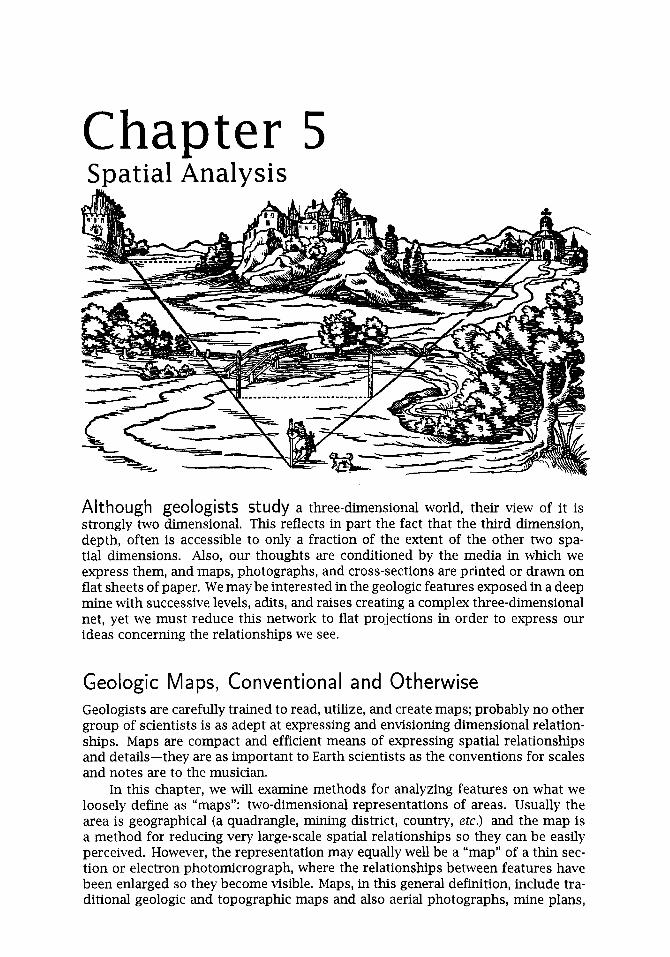
Chapter 5 Spatial Analysis
Although geologists study a three-dimensional world, their view of it is strongly two dimensional. This reflects in part the fact that the third dimension, depth, often is accessible to only a fraction of the extent of the other two spa- tial dimensions. Also, our thoughts are conditioned by the media in which we express them, and maps, photographs, and cross-sections are printed or drawn on flat sheets of paper. We may be interested in the geologic features exposed in a deep mine with successive levels, adits, and raises creating a complex three-dimensional net, yet we must reduce this network to flat projections in order to express our ideas concerning the relationships we see.
Geologic Maps, Conventional and Otherwise Geologists are carefully trained to read, utilize, and create maps; probably no other group of scientists is as adept at expressing and envisioning dimensional relation- ships. Maps are compact and efficient means of expressing spatial relationships and details-they are as important to Earth scientists as the conventions for scales and notes are to the musician.
In this chapter, we will examine methods for analyzing features on what we loosely define as “maps”: two-dimensional representations of areas. Usually the area is geographical (a quadrangle, mining district, country, etc.) and the map is a method for reducing very large-scale spatial relationships so they can be easily perceived. However, the representation may equally well be a “map” of a thin sec- tion or electron photomicrograph, where the relationships between features have been enlarged so they become visible. Maps, in this general definition, include tra- ditional geologic and topographic maps and also aerial photographs, mine plans,

Statistics and Data Analysis in Geology - Chapter 5
peel prints, photomicrographs, and electron micrographs. In fact, any sort of two- dimensional spatial representation is included.
Among the topics we will consider that have obvious applications to fields as diverse as geophysics and microscopy is the probability of encountering an object with a systematic search across an area. We will look at the statistics of directional data in both two and three dimensions. Many natural phenomena are expressed as complicated patterns of lines and areas that can best be described as fractals, which we will touch upon. We will also look at ways of describing and comparing more conventional shapes of individual objects, ranging in size from islands to oil fields to microfossils.
Map relationships are almost always expressed in terms of points located on the map. We are concerned with distances between points, the density of points, and the values assigned to points. Most maps are estimates of continuous func- tions based on observations made at discrete points. An obvious example is the topographic map; although the contour lines are an expression of a continuous and unbroken surface, the lines are calculated from measurements taken at trian- gulation and survey control points. An even more obvious example is a structural contour map. We do not know that the structural surface is continuous, because we can observe it only at the locations where drill holes penetrate the surface. Nevertheless, we believe that it is continuous and we estimate its form from the measurements made at the wells, recognizing that our reconstruction is inaccurate and lacking in detail because we have no data between wells.
When mapping the surface geology of a desert region, we can stand at one locality where strike and dip have been measured and extend formation bound- aries on our map with great assurance because we can see the contacts across the countryside. In regions of heavy vegetation or deep weathering, however, we must make do with scattered outcrops and poor exposures; the quality of the finished map reflects to a great extent the density of control points. Geologists should be intensely interested in the effects which control-point distributions have on maps, but few studies of this influence have been published. In fact, almost all studies of point distributions have been made by geographers. In this chapter, we will exam- ine some of these procedures and consider their application to maps and also to such problems as the distribution of mineral grains in thin sections.
Geologists exercise their artistic talents as well as their geologic skills when they create contour maps. In some instances, the addition of geologic interpre- tation to the raw data contained in the observation points is a valuable enhance- ment of the map. Sometimes, however, geologic judgment becomes biased, and the subtle effects of personal opinion detract rather than add to the utility of a map. Computer contouring is totally consistent and provides a counterbalance to overly interpretative traditional mapping. Of course, subjective judgment is necessary in choosing an algorithm to perform mapping, but methods are available that allow a choice to be made between competing algorithms, based upon specified criteria. The principal motive behind the development of automatic contouring is economic, an attempt to utilize the petroleum industry’s vast investment in stratigraphic data banks. Aside from this, one of the prime benefits of computerized mapping tech- niques may come from the attention they focus on the contouring process and the problems they reveal about map reliability. Contour mapping is the subject of one section in this chapter.
Trend-surface analysis is a popular numerical technique in geology. However, although it is widely applied, it is frequently misused. Therefore, we will discuss
294

Spat ia I Ana I ysis
the problems of data-point distribution, lack of fit, computational “blowup,” and inappropriate applications. Statistical tests are available for trend surfaces if they are to be used as multiple regressions; we will consider these tests and the assump- tions prerequisite to their application.
The exchange between Earth scientists and statisticians has been mostly one way, with the notable exception of the expansion of the theory of regionalized vari- ables. This theory, developed originally by Georges Matheron, a French mining engineer, describes the statistical behavior of spatial properties that are interme- diate between purely random and completely deterministic phenomena. The most familiar application of the theory is in kriging, an estimation procedure important in mine evaluation, mapping, and other applications where values of a property must be estimated at specific geographic locations.
Two-dimensional methods are, for the most part, direct extensions of tech- niques discussed in Chapter 4. Trend-surface analysis is an offshoot of statistical regression; kriging is related to time-series analysis; contouring is an extension of interpolation procedures. We have simply enlarged the dimensionality of the subjects of our inquiries by considering a second (and in some cases a third) spa- tial variable. Of course, there are some applications and some analytical meth- ods that are unique to map analysis. Other methods are a subset of more general multidimensional procedures. It is an indication of the importance of one- and two-dimensional problems in the Earth sciences that they have been included in individual chapters.
Systematic Patterns of Search Most geologists devote their professional careers to the process of searching for something hidden. Usually the object of the search is an undiscovered oil field or an ore body, but for some it may be a flaw in a casting, a primate fossil in an excavation, or a thermal spring on the ocean’s floor. Too often the search has been conducted haphazardly-the geologist wanders at random across the area of investigation like an old-time prospector following his burro. Increasingly, how- ever, geologists and other Earth scientists are using systematic procedures to search, particularly when they must rely on instruments to detect their targets.
Most systematic searches are conducted along one or more sets of parallel lines. Ore bodies that are distinctively radioactive or magnetic are sought using airborne instruments carried along equally spaced parallel flight lines. Seismic surveys are laid out in regular sets of traverses. Satellite reconnaissance, by its very nature, consists of parallel orbital tracks.
The probabilities that targets will be detected by a search along a set of lines can be determined by geometrical considerations. Basically, the probability of dis- covery is related to the relative size of the target as compared to the spacing of the search pattern. The shape of the target and the arrangement of the lines of search also influence the probability. If the target is assumed to be elliptical and the search consists of parallel lines, the probability that a line will intersect a hidden target of specified size, regardless of where it occurs within the search area, can be calculated. These assumptions do not seem unreasonable for many exploratory surveys. Note that the probabilities relate only to intersecting a target with a line, and do not consider the problem of recognizing a target when it is hit.
McCammon (1977) gives the derivation of the geometric probabilities for cir- cular and linear targets and parallel-line searches. His work is based mostly on the
295

Statistics and Data Analysis in Geology - Chapter 5
mathematical development of Kendall and Moran (1963). An older text by Uspensky (1937) derives the more general elliptical case used here.
Assume the target being sought is an ellipse whose dimensions are given by the major semiaxis u and minor semiaxis b. (If the target is circular, then u = b = r, the radius of the circle.) The search pattern consists of a series of parallel traverses spaced a distance D apart (Fig. 5-1 a). The probability that a target (smaller than the spacing between lines) will be intersected by a line is
D p = -
7TD where P is the perimeter of the elliptical target. The equation for the perimeter of an ellipse is P = 2 7 ~ d m , where u and b are the major and minor semiaxes. Substituting,
2 T I p q z - 2 J q F (5.2) - -
’= ~ T D D
We can define a quantity Q as the numerator of Equation (5.2); that is, Q = 24(u* + b2)/2. With this simplification, the probability of intersecting an elliptical target with one line in a set of parallel search lines can be written as
p = - Q D (5.3)
In the specific case of a circular target, u and b are both equal to the radius, so Q can be replaced by twice the radius:
2r p = - D (5.4)
At the other extreme, one axis of the ellipse may be so short that the target becomes a randomly oriented line. This geometric relationship is known as Bwffon’s problem, which specifies the probability that a needle of length 8, when dropped at random on a set of ruled lines having a spacing D , will fall across one of the lines. The probability is
28 p = - 7TD (5.5)
where 4? is the length of the target. A similar geometric relationship, known as Laplace’s problem, also pertains to
the probabilities in systematic searches. Laplace’s problem specifies the probability that a needle of length 8, when dropped on a board covered with a set of rectangles, will lie entirely within a single rectangle. A variant gives the probability that a coin tossed onto a chessboard will fall entirely within one square. In exploration, the complementary probabilities are of interest, i.e., that a randomly located target will be intersected one or more times by a set of lines, such as seismic traverses, arranged in a rectangular grid (Fig. 5-1 b).
The general equation is
where D1 is the spacing between one set of parallel seismic traverses and DZ is the spacing between the perpendicular set of traverses. In the specific instance of a
296

Spat ia I Ana I ysis
Figure 5-1. Search for an elliptical target with major semiaxis a and minor semiaxis b. (a) Using a parallel-line search of spacing D . ( b ) Using a grid search with spacing D1 in one direction and Dz in the perpendicular direction.
Figure 5-2. Probability of intersecting a target with a systematic pattern of search. Shape of target may range from a circle to a line; elliptical targets of various axial ratios fall in the shaded region. Horizontal axis is ratio (major dimension of target)/(spacing between search lines). (a) Parallel-line search pattern. (b ) Square-grid search pat- tern. After McCammon (1977).
297

Statistics and Data Analysis in Geology- Chapter 5
search in the pattern of a square grid, the equation simplifies to
Lambie (unpublished report, 1981) has pointed out that these equations for geometric probability are approximations of integral equations. Comparing exact probabilities found by numerical integration with those predicted by the approxi- mation equations, he found that significant differences occur only for very elongate targets that are large with respect to spacing between search lines. Then, equations such as (5.3) and (5.6) may seriously overestimate the probabilities of detection.
The probabilities of intersecting a target, as calculated by the approximating equations, can be shown conveniently as graphs. McCammon (1977) presented such graphs in a particularly useful dimensionless form for various combinations of tar- get shape and size relative to the spacing between the search lines. Figure 5-2a gives the probability of detecting an elliptical target whose shape ranges from a circle to a line, using a search pattern of parallel lines. The relative size of the target is found by dividing the target's maximum dimension by the search line
Figure 5-3. Probability of intersecting targets with regular search patterns ranging from squares to parallel lines. Rectangular search patterns with different ratios of D1 /D2 fal l in the shaded region. Horizontal axis is ratio fmaior dimension of targetl/fmini- mum spacing betwe& search lines). (a) Target is'cir&lar, ( b ) Target is a"li<e.'After McCammon (1977).

Spa t ia I Analysis
spacing. Figure 5-2 b is an equivalent graph for a search pattern consisting of a square grid of lines.
If the shape of the target is specified, the probabilities of intersection can be graphed for different patterns of search. Figure 5-3 a, for example, shows the prob- ability of intersecting a circular target with search patterns ranging from a square grid, through rectangular grid patterns, to a parallel-line search. Figure 5-3 b is the equivalent graph for a line-shaped target. Between the two graphs, all possible shapes of elliptical targets and all possible patterns of search along two perpendic- ular sets of parallel lines are encompassed.
Distribution of Points Geologists often are interested in the manner in which points are distributed on a two-dimensional surface or a map. The points may represent sample localities, oil wells, control points, or poles and projections on a stereonet. We may be concerned about the uniformity of control-point coverage, the distribution of point density, or the relation of one point to another. These are questions of intense interest to geographers as well as geologists, and the burgeoning field of locational analysis is devoted to these and similar problems. Although much of the attention of the geographer is focused on the distribution of shopping malls or public facilities, the methodologies are directly applicable to the study of natural phenomena as well.
The patterns of points on maps may be conveniently classified into three categories: regular, random, and aggregated or clustered. Examples of point dis- tributions are shown in Figure 5-4 and range from the most uniform possible (the face-centered hexagonal lattice in Fig. 5-4a, where every point is equidistant from its six nearest neighbors) to a highly clustered pattern composed of randomly lo- cated centers around which the probability of occurrence of a point decreases exponentially with distance (Fig. 5-4f). Of course most maps will have patterns intermediate between these extremes, and the problem becomes one of determin- ing where the observed pattern lies within the spectrum of possible distributions. For example, most people would intuitively regard the distribution of points in Figure 5 - 4 c as random. However, intuition is wrong, because the map was created by dividing the map area into a 4 x 4 array of regular cells and then placing four points at random within each cell (except in the shortened bottom row, which re- ceived only two points per cell). The distribution therefore has both random and regular aspects and is more uniform in density than a purely random arrangement such as Figure 5-4d.
The pattern of points on a map is said to be uniform if the density of points in any subarea is equal to the density of points in all other subareas of the same size and shape. The pattern is regular if the spacings between points repeat, as on a grid. That is, the distance between a point i and another point j lying in some specified direction from i is the same for all pairs of points i and j on the map. Obviously, a regular pattern also will be uniform, but the converse is not necessarily true. A random pattern can be created if any subarea is as likely to contain a point as any other subarea of the same size, regardless of the subarea’s location, and the placement of a point has no influence on the placement of any other point. In an aggregated or clustered pattern, the probability of occurrence of a point varies in some inverse manner with distances to preexisting points.
299

Statistics and Data Analysis in Geology - Chapter 5
0 0 0 0 0 0 0 0
0 0 0 0 0 0 0 0
0 0 0 0 0 0 0 0
0 0 0 0 0 0 0
0 0 0 0 0 0 0
0 0 0 0 0 0 0
0 0 0 0 0 0 0
0 0 0 0 0 0 0
0 0 0 0 0 0 0
0 0 0 0 0 0 0
0 0 0 0 0 0 0 I U
0 0 0 0 0 O 0 0 0 0
0 O O O 0 0
o o o o o o 0
- 0 0 0 O o o
0 0 0 0 0 0 0 0 0 o o O ,"I 0 0 0 0 0 0 0 OI 0 IiOo o o 0 0 0
0 0 0 0 0 0 0 0 I l o o 0 0 O 0 0 01
0 0 0 0 0 0 0 01 j o o o o o o 0 1 0 - b C
d e
Figure 5-4. Some possible patterns of points on maps. Each map contains 56 points. (a ) Points regularly spaced on a face-centered hexagonal grid or network. Every point is equidistant from six other points. (b ) Points regularly arranged on a square grid. (c) Sets of four points placed randomly within each cell of a regular 4 x 4 grid. The bottom row contains only two points per cell. ( d ) Points located by a bivariate uniform random process. (e ) Nonuniform pattern of points produced by logarithmic scaling of the X-axis. ( f ) Points located by randomly placing seven cluster centers (black points) and moving eight points a random direction and logarithmically scaled distance from each center.
A uniform density of data points is important in many types of analysis, includ- ing trend-surface methods which we will discuss later. The reliability of contour maps is directly dependent upon the total density of control points as well as their uniformity of distribution. However, most geologic researchers have been content with qualitative judgments of the adequacy and representativeness of the distribu- tion of their data. Even though the desirability of a uniform density of observations is often cited, the degree of uniformity is seldom measured. The tests necessary to determine uniformity are very simple, and it is unfortunate that many geologists seem unaware of them. These tests are, however, extensively used by geographers. Haggett, Cliff, and Frey (1977); Getis and Boots (1978); Cliff and Ord (1981); and Bailey and Gatrell(l995) provide an introduction to this literature.
Uniform density .A map area may be divided into a number of equal-sized subareas (sometimes called quadrats) such that each subarea contains a number of points. If the data points are distributed uniformly, we expect each subarea to contain the same num- ber of points. This hypothesis of no difference in the number of points per subarea (:an be tested using a x 2 method, and is theoretically independent of the shape or
300

Spatial Analysis
0
0
0 0
0
0 0 0
5 4 O O
0 0 0
0 (1 0
U
0
10
0 C
% 1 5 - L - 0 z
I o c
I
" 0 %
m o 0 0
0 0 00 0
0 " 0 0 0 0 0 0 0 0
0 0
0
0 0
0 0 3 0 0 0
0 254 0
0 o o O U
1 5 20
0 000 0 m
U
0 0
0 O;I 0 0
00 b
0
b 2 5 3 0 3 5 40
Easting
Figure 5-5. Locations of 123 exploratory holes drilled to top of Ordovician rocks (Arbuckle Group) in central Kansas. Map has been divided into 12 cells of equal size.
orientation of subareas. However, the test is most efficient if the number of subar- eas is a maximum (this increases the degrees of freedom), subject to the restriction that no subarea contain fewer than five points. The expected number of points in each subarea is N
k (5 .8) E = -
where N is the total number of data points and k is the number of subareas. A x 2 test of goodness of fit of the observed distribution to the expected (uniform) distribution is
where Oi is the observed number of data points in subarea i and E is the expected number. The test has v = k - 2 degrees of freedom, where k is the number of subareas.
As an example of the application of this test, consider the data-point distribu- tion shown in Figure 5-5. These are the locations of 123 holes drilled in the search for oil in the Ordovician Arbuckle stratigraphic succession in central Kansas. These data are listed in file ARBUCKLE.TXT. In Figure 5-5, the map area has been divided into 12 equal subareas, each of which we expect to contain about ten points, if the points are uniformly distributed. The observed number of points in each subarea and the computations necessary to find the test value are given in Table 5-1. This test has v = 10 degrees of freedom, so the critical value of x 2 at the 5% (a = 0.05) significance level is 18.3. The computed test value of x 2 = 17.0 does not exceed
301

Statistics and Data Analysis in Geology - Chapter 5
this, so we conclude that there is no evidence suggesting that the quadrats are unevenly populated. Note that the test applies only to the uniformity of point den- sities between areas of a specified size and shape. It is possible that we could select quadrats of different sizes or shapes that might not be uniformly populated, especially if they were smaller than those used in this test.
Table 5-1. Number of wells in 12 subareas of central Kansas.
Observed Number (0 - E ) * of Points E
10 0.006 5 2.689 5 2.689
11 0.055 13 0.738
5 2.689 12 0.299 16 3.226 16 3.226 9 0.152
13 0.738 8 0.494
TOTAL = 123
aTest value is not significant at the a = 0.05 level.
x 2 = 16.995"
Random patterns Establishing that a pattern is uniform does not specify the nature of the unifor- mity, for both regular and random patterns are expected to be homogeneous. For many purposes, verifying uniformity is sufficient; but, if we desire more informa- tion about the pattern, we must turn to other tests. If points are distributed at random across a map area, even though the coverage is uniform, we do not expect exactly the same number of points to lie within each subarea. Rather, there will be some preferred number of points that occur in most subareas and there will be progressively fewer subareas that contain either more points or fewer. This is apparent in the example we just worked: although our hypothesis of uniformity specified that we expect about ten observations in each subarea, we actually found some areas that contained more than ten and some that contained fewer.
You will recall that the Poisson probability distribution is the limiting case of the binomial distribution when p , the probability of a success, is very small and (1 - p ) approaches 1.0. The Poisson distribution can be used to model the occurrence of rare, random occurrences in time, as it was used in Chapter 4, or it can be used to model the random placement of points in space. Although the Poisson distribution, like the binomial, uses the numbers of successes, failures, and trials in the calculation of probabilities, it can be rewritten so that neither the number of failures nor the total number of trials is required. Rather, it uses the number of points per quadrat and the density of points in the entire area to predict how many quadrats should contain specified numbers of points. These predicted
302

Spat ia I An a I ysis
or expected numbers of quadrats can be used in a x 2 procedure to test whether the points are distributed at random within the area.
As an application, we can determine if oil discoveries in a basin occur at ran- dom or are distributed in some other fashion. It is not intuitively obvious that the Poisson distribution can be expressed in a form appropriate for this problem, so we will work through its development.
Assume a basin has an area, a, in which m discovery wells are randomly lo- cated. The density of discovery wells in the basin is designated A, and is simply
712 A = - a (5.10)
The basin may be divided into small lease tracts, each of area A (here the term “tract” is equivalent to “quadrat”). In turn, each tract may be divided into n extremely small, equal-sized subareas which we might regard as potential drilling sites. The probability that any one of these extremely small subareas contains a discovery well tends toward zero as n becomes infinitely large.
The area of each drilling site is Aln. The probability that a site contains a discoverv well is
and the probability that it does not contain a discovery well is
1 - p = 1 - A - ( 3 We wish to investigate the probability that Y of the n drilling sites within a
tract contain discovery wells, and n - Y drilling sites do not. The probability of a specific combination of discovery and nondiscovery well sites within a tract is
P = ( A ; ) r (1 - A;).-.
However, within a tract, there are (:) combinations of the n drilling sites, of which Y contain discovery wells and all are equally probable. The probability that a tract will contain exactly Y discovery wells is therefore
P (Y) = (;) ( A : ) r (1 - A:).-.
Note that this is simply the binomial probability of Y discovery wells on n drilling sites.
The combinations can be expanded into factorials,
n ( n - 1) (n- 2) * . . (n -Y + 1) (AA)’ AA P ( Y ) = r ! nr
Rearranging and canceling terms yields
P (Y) = (1 - i) (1 - f) ... (1 - G) (1 - q) AA -‘ [(I - --) AA 71 (AA)‘ (5.11)
303

Statistics and Data Analysis in Geology - Chapter 5
As n becomes infinitely large, all of the fractions that contain n in their denominator become infinitesimally small and vanish, so all terms inside parentheses simply become equal to 1. The terms inside the brackets simplify to
(-AA) P ( r ) = e r! (5.12)
Note that n, the number of drilling sites, has vanished from the equation leaving only the discovery-well density, A, the number of discovery wells, Y, and the area, A, of the tracts. This is an expression of the Poisson distribution, as applied to the probability of rare, random events (discovery wells) occurring within geographic areas. Also note that AA is simply the mean number of wells per tract, because it is the product of the density of discovery wells times the area of a tract. In practice, we estimate AA from the total number of discovery wells, m, and the total number of tracts, T m h A = -
T (5.13)
We can now perform a x 2 test to see if the number of wells per tract matches that expected if the wells are randomly located according to the Poisson model. The number of tracts that contain exactly r discovery wells can be found by
nr = mP(r)
( - h A ) = me r! If AA is estimated by m / T , the equation becomes
(5.14)
(5.15)
Figure 5-6 shows the locations of discovery wells in part of the Eastern Shelf area of the Permian Basin in Fisher and Noland counties of Texas. The area has been divided into a l o x 16 grid of 160 tracts, or quadrats, each containing approximately 10 mi2. Since there are 168 discovery wells in the area, the mean number of wells per tract is
m 168 T 160
= 1.05 - = -
We can count the number of tracts in the map that contain no discovery wells, exactly one discovery, two discoveries, and so forth. Using Equation (5 .15) , we can also calculate the expected number of tracts that contain these same numbers of wells. The expected and observed numbers of tracts for the Permian Basin area are given in Table 5-2. This table contains all of the figures necessary to calculate a x2 test of goodness of fit, which is essentially a comparison of the two histograms shown in Figure 5-7. The last three categories must be combined so that the ob- served number of tracts is equal to or greater than five
70 - 56.0)’ (42 - 58.8)’ + (26 - 30.9)’ 58.8 30.9
2 J + - 56.0
= 13.28 (17 - 10.8)’ + ( 5 - 3.5)2
10.8 3.5 + ‘The test statistic has c - 2 degrees of freedom, where c is the number of categories (one degree of freedom is lost because the expected frequencies are constrained
304

Spatial Analysis
to sum to 160, and a second degree of freedom is required for estimation of the parameter A). For c = 5 categories, there are three degrees of freedom.
Figure 5-6. Locations o f oil-field discovery wells in part o f the Eastern Shelf area o f the Permian Basin, Fisher and Noland counties, Texas. Quadrats are approximately 10 mi2 in size.
Table 5-2. Calculation o f expected numbers of tracts containing Y discoveries in eastern part of Permian Basin, Texas, assuming a Poisson distribution.
Number of Discoveries
Number of Tracts Tract Contains
Per Tract (Y) Poisson Eauation Y Discoveries m e c t e d Observed
0 q0) = e(-1.05)1.050 O! 0.3499
1 p(l) = e(-1.05).!& l! 0.3674
2 p ( 2 ) = e(-1.05)* 2! 0.1929
3
4 q4) = e(-1.05)1.054 4! 0.0177
5 q5) = e(-1.05)1.055 5 ! 0.0037
6 p ( @ = e(-1.05)1.056 6! 0.0007 TOTALS 0.9998
p ( 3 ) = e ( - 1 . 0 5 ) W 0.0675 3!
56.0 70
58.8 42
30.9 26
10.8 17
2.8 3
0.6 1
0.1 __ 1 160.0 160
305

Statistics and Data Analysis in Geology - Chapter 5
Figure 5-7. Histograms showing observed numbers of discovery wells per tract in an area of the Permian Basin, and the number expected if fields are distributed randomly according to a Poisson model.
The critical value of x 2 for v = 3 and (x = 0.05 is 7.81. The test statistic far exceeds this value, so we must reject the hypothesis of equality between the observed and expected distributions and conclude that the Poisson model is not appropriate. Oil discoveries have not been made randomly within this area of the Permian Basin.
In the process of fitting the Poisson model to this data, we have generated some information that may provide additional insight into the nature of the spatial distribution. The mean number of discoveries per tract is estimated by Equation (5.13). The variance in number of discoveries per tract is
(5.16)
where ri is the number of discoveries in the i t h tract. The summation extends over all T tracts. The alternative results of comparing the estimated mean and variance are
m / T > s2 m / T = s2 Pattern random m / T < s2
Pattern more uniform than random
Pattern more clustered than random
Of course, some difference between m l T and s2 may arise due to random variation in the particular set of tracts chosen. The statistical significance of the observed difference may be tested by a t-test based on the standard error of the mean, which is the variance that would be expected in values of m / T if a basin were repeatedly sampled by different sets of tracts of the same size. The standard error in the mean number of discoveries per tract is
306
(5.17)

Spatial Analysis
The t-test compares the ratio between m / T and s2, which should be equal to 1.0 if the two statistics are the same
(F) - 1.0 t =
Se (5.18)
The test has T - 1 degrees of freedom. For the eastern Permian Basin area, the variance in number of wells per tract is
The standard error of the mean number of wells per tract can be estimated as
se = & = 0.112
The t-statistic for the test of equivalence of the mean and variance is
(1.05/1.46) - 1.0 0.112 = -8.86 t =
At a significance level of o( = 0.05 and 159 degrees of freedom, the critical value of t for a two-tailed test is 1.96; the computed statistic far exceeds this and so we may conclude as we did in the x2 test that the spatial distribution is not random. Since the variance is significantly greater than the mean, we must also conclude that discovery wells are areally clustered.
CI ustered patterns Many naturally occurring spatial distributions show a pronounced tendency toward clustering. This is especially true of certain biological variables, such as presence of specific organisms or occurrences of an infectious disease. The descendants of a sedentary parent, perhaps a coral or a tree, tend to grow nearby, leading to devel- opment of densely populated areas surrounded by areas that are relatively barren. Clustered patterns of points can be modeled by many theoretical distributions, most of which can be regarded as combinations of two or more simpler distribu- tions. One of the distributions describes the locations of the centers of clusters, while the other describes the pattern of individual points around the centers of the clusters.
The negative binomial distribution can be used to model the occurrence of clustered points in space in a manner equivalent to the use of the Poisson to model randomly arranged points. An extensive discussion with citations to studies in many fields is given by Ripley (1981). Griffiths (1962, 1966) advocated the use of the negative binomial as an appropriate model for the occurrence of oil fields and ore bodies.
One derivation of the negative binomial is as a compound Poisson and loga- rithmic distribution with clusters of points randomly located within a region; indi- vidual points within a cluster follow a logarithmic distribution. In the formulation appropriate for describing spatial patterns, the negative binomial is
k (5.19)
307

Statistics and Data Analysis in Geology - Chapter 5
In terms of the oil-field distribution problem we have just considered, Y is the number of discovery wells in a tract, p is the probability that a given drilling site contains a discovery well, and k is a measure of the degree of clustering of the discoveries. If k is large, clustering is less pronounced and the spatial distribution approaches the Poisson, or randomness. As k approaches zero, the pattern of clustering becomes more pronounced. The density, A, is equal to
h = k p (5.20)
If k is not an integer (and in general it will not be), this combinatorial equation cannot be solved. Then, the following approximation must be used:
(5.21)
As with the Poisson distribution, h is estimated by the average density of discoveries per tract, m / T . The clustering parameter, k , is estimated by
(5.22)
where s2 is the variance in number of discovery wells per tract. Then, the probability p can be estimated as
(5.23)
We can apply the negative binomial model to the data on discovery wells in the eastern part of the Permian Basin (Fig. 5-6) to see if this distribution can ade- quately describe their spatial distribution. The mean and variance of the number of discovery wells per tract have already been found: m / T = .1.05 and s2 = 1.46. The clustering effect can be estimated using Equation (5.22)
= 2.69 1.05* k = 1.46 - 1.05
In turn, the probability of a discovery well occurring in a tract is
p = - - "05 - 0.390 2.69
Using the approximation equations, the probability that a given tract will con- tain no discovery wells is
= 0.4124 1
(1 + 0.390)2.69 P ( 0 ) =
The probability that a tract will contain exactly one discovery well is
308

Spatial Analysis
Table 5-3. Expected numbers of tracts containing Y discoveries in eastern part of Permian Basin, Texas, assuming a negative binomial distribution.
Probability Number of Tracts Number of Discoveries Tract Contains Per Tract (Y) Y Discoveries Expected Observed
0 1 2 3 4 5 6
TOTALS
0.4124 0.3112 0.1611 0.0706 0.0281 0.0106 0.0038 0.9988
66.0 49.8 25.8 11.3 4.5 1.7 0.6
159.7
70 42 26 17
3 1 2 160
Discovery wells per tract
Figure 5-8. Histograms showing observed numbers of discovery wells per tract in an area of the Permian Basin, and the number expected in a clustered (negative binomial) model.
The probabilities that a tract will contain exactly two, three, or other num- ber of discovery wells can be calculated in a similar fashion. Then, the expected number of tracts containing Y discoveries can be determined simply by multiplying these probabilities by 160, the total number of tracts. Table 5-3 gives the expected numbers of tracts for up to six discoveries per tract.
The numbers of tracts containing exactly Y discoveries as predicted by the negative binomial model are compared to the corresponding observed numbers of tracts in Figure 5-8. The goodness of fit of the negative binomial can be tested by
309

Statistics and Data Analysis in Geology - Chapter 5
a x 2 test exactly like that used to check the fit of the Poisson model. Again, it is necessary to combine the final three categories so a frequency of five or more is obtained. The test statistic is x 2 = 4.82, with (5 - 2 = 3) degrees of freedom. This is less than the critical value of x 2 for o( = 0.05 and v = 3, so we cannot reject the negative binomial as a model of the spatial distribution of discovery wells in the eastern part of the Permian Basin. Keep in mind that this is not equivalent to proof that the wells do follow a negative binomial model, because it is possible that some other clustered model might provide an even better fit. However, the negative binomial does generate a spatial distribution that is statistically indistinguishable from the one observed.
Nearest- neig h bor an a lysis An alternative to quadrat analysis is nearest-neighbor analysis. The data used are not the numbers of points within subareas, but the distances between closest pairs of points. Since it is not necessary to select a quadrat size, nearest-neighbor pro- cedures avoid the possibility of finding that a pattern is random at one scale but not at another. Also, since there are usually many more pairs of nearest neigh- bors than quadrats, the analysis is more sensitive. A good introduction to nearest- neighbor techniques is given by Getis and Boots (1978). Ripley (1981) provides a review of theory and applications in several fields, as do Cliff and Ord (1981). Shaw and Wheeler (1994) and B&ley and Gatrell(1995) discuss computational aspects of neares t-neighbor analyses.
Nearest-neighbor analysis compares characteristics of the observed set of dis- tances between pairs of nearest points with those that would be expected if the points were randomly placed. The characteristics of a theoretical random pattern can be derived from the Poisson distribution. If we ignore the effect of the edges of our map, the expected mean distance between nearest neighbors is
- 1 s ’ 2 m (5.24)
where A is the area of the map and n is the number of points. You will recall that A / n is the point density, A. The sampling variance of is given by
If we work out the constants.
0.06831 A n2
g; =
(5.25)
(5.26)
The standard error of the mean distance between nearest neighbors is the square root of CT;
0.26136 se = 4- (5.27)
The distribution of simple z-test given
- 6 is normal provided n is greater than 6, so we can use the in Chapter 2 to test the hypothesis that the observed mean
310

Spat ia I An a I ysis
distance between nearest neighbors, a, is equal to the value of 8 from a random pattern of points of the same density. The test is
- d - 8 z = -
Se (5.28)
This is the form of the nearest-neighbor test that is commonly presented, but un- - fortunately it has a serious defect for most practical purposes. The expected value 6 assumes that edge effects are not present, which means that the observed pattern of points must extend to infinity in all directions if a and 8 are to be validly com- pared. Since the map does not extend indefinitely, the nearest neighbors of points near the edges must lie within the body of the map, and so d is biased toward a greater value (Upton and Fingleton, 1985). There are several corrections for this problem. If data are available beyond the limits of the area being analyzed, the map can be surrounded by a guard region. Then, nearest-neighbor distances be- tween points inside the map and points in the guard region can be included in the calculation of d. Alternatively, we can consider our map to be drawn not on a flat plane but on a torus. In this case, in the right map edge would be adjacent to the left edge and the top adjacent to the bottom. The nearest neighbor of a point along the right edge of the map might lie just inside the left edge (this concept should be familiar to anyone who has contoured point densities on stereonets). Another way of regarding this particular correction is to imagine that the pattern of points repeats in all directions, like floor tiles. Any point lying adjacent to an edge of the map has {he opportunity to find a point across the edge that may be a closer neighbor than the nearest point within the map.
A third correction involves adjusting d so that the boundary effects are in- cluded in its expected value. Using numerical simulation, Donnelly (1978) found these alternative expressions for the theoretical mean nearest-neighbor distance and its sampling variance:
and 58 N 0.070- A + 0 . 0 3 5 P p J A
n2
(5.29)
(5.30)
In these approximations, p is the perimeter of the rectangular map. Note that if the map has no edges, as when it is considered to be drawn on a torus, p is zero and these equations are identical to equations (5.24) and (5.26):
The expected and observed mean nearest-neighbor distances can be used to construct an index to the spatial pattern. The ratio
- d 6
R = - (5.31)
is the nearest-neighbor statistic and ranges from 0.0 for a distribution where all points coincide and are separated by distances of zero, to 1.0 for a random dis- tribution of points, to a maximum value of 2.15. The latter value characterizes a distribution in which the mean distance to the nearest neighbor is maximized. The distribution has the form of a regular hexagonal pattern where every point
311

Statistics and Data Analysis in Geology - Chapter 5
00 0 % 0 00 00
0 0 o o o o o o
0 0 0
0 008 oo $ 0
0 0 0
O O 0 0 0 0
00 0 B o O O O 0 0 0
0 O O 00 0 0
0 0 O n
0 0
0 0
0 0
0 0
0 0
0 0
0 0 0 0
0 0 0 0
0 0
0
0 0
0
0 0
0 0 0 0
a -
0 0 0 0
00 0 O O
o oe
0 0 O
0 0
0 0
0 0 0
0 0 0 0 O Q
0 D O 0
0 0 cDo 0 n - a
0 0 0 0 0 0 0 0
0 0 0 0 0 0 0 0
0 0 0 0 0 0 0 0
0 0 0 0 0 0 0 0
0 0 0 0 0 0 0 0
0 0 0 0 0 0 0 0
0 0 0 0 0 0 0 0
0 0 0 0 0 0 0 0
b
%
0 0 0 8
f
Figure 5-9. Nearest-neighbor statistics, R , for patterns of points on maps. (a) Points in a regular hexagonal network, R = 2.15. (b ) Points in a regular square network, R = 2.00. (c) Points placed randomly within regular hexagonal cells, R = 1.26. ( d ) Points placed a t random locations, R = 0.91. (e) Points placed randomly within five random clusters, R = 0.34. ( f ) Points placed randomly within a single cluster, R = 0.13. Point density, A , is the same for all patterns. From Olea (1982).
is equidistant from six other points. Figure 5-9 shows a series of patterns with different values of the nearest-neighbor statistic, all having the same point density.
We will illustrate the application of the nearest-neighbor method using the map shown in Figure 5-10. The “map” actually represents a polished facing stone on the front of a bank in a university town. It provides an interesting subject of study for an igneous petrology class. The stone is black anorthosite and contains small, scattered, euhedral crystals of magnetite. The instructor uses the slab to demon- strate a variety of topics, including examples of numerical techniques in petrog- raphy. For pedagogical purposes, it has been decreed that the slab is mounted in its original orientation. That is, it represents a vertical surface; “down” is to- ward the bottom of the slab. The map shows the location of all visible magnetite grains on the surface. Coordinates of each grain, in centimeters from the lower left corner of the slab, are listed in file BANK.TXT. Are magnetite grains uniformly distributed across the surface, or do they tend to be clustered? Is the density of crystals greater near the bottom of the slab than near the top? These and similar questions are of great importance in determining the petrogenesis of an igneous rock, and can be effectively investigated using the techniques we have discussed. Test the hypothesis of uniform, random distribution of crystals by both quadrat and nearest-neighbor analysis. This problem may be done by hand by measuring distances directly on Figure 5-10, or the distances may be computed using the
312

Spat i a I An a I ysis
100-
-
80-
-
60 - r I
.- E - Y S s
40-
-
20-
-
O J
4 4
4
4
4 1
4
' 4 ' 4 4 4 4 4 4
4
4
t
4'
4
4 4
4
4
4
4 4
4 4 4
4 4
4
Figure 5-10. Representation of a polished slab of anorthosite facing stone showing locations of magnetite crystals listed in file BANK.TXT.
coordinates in file BANK.TXT. Ripley (1981, p. 175-181) gives an exhaustive analy- sis of these data, using a variety of techniques.
Distribution of Lines Some naturally occurring patterns are composed of lines, such as lineaments seen on satellite images, the tracery of joints exposed on a weathered granite surface, or the microfractures seen in a thin section of a deformed rock. Just as a set of points can form a pattern that ranges from uniform to tightly clustered, so can sets of lines. Of course, lines are more complex than points because they pos- sess length and orientation, as well as location. Their analysis is correspondingly more difficult, and statistical methods suitable for the study of patterns of lines seem less well developed than those applied to patterns of points. Few studies have examined the distribution of lengths of lines, except for some work on the lognormal distribution (Aitchison and Brown, 1969). A small number of workers have investigated the spacing between lines in a pattern, a problem analogous to nearest-neighbor analysis of points (Miles, 1964; Dacey, 1967). A much larger body of literature exists on the orientation of lines, a topic we will consider in the next section.
We can define a random pattern of lines as one in which any line is equally likely to cross any location, and any orientation of the crossing line is also equally likely. Such random patterns can be generated in many ways; one procedure consists of
313

Statistics and Data Analysis in Geology - Chapter 5
I
%/
Figure 5-11. Calculation of nearest-neighbor distances between lines. Point p is chosen a t random on a line X . Dashed lines U , b, and c are perpendiculars drawn from point p t o nearby lines. The shortest o f these, perpendicular line c, is the distance t o the nearest neighbor of line X . The process is repeated t o find the nearest-neighbor distances for all lines.
choosing two pairs of coordinates from a random number table, then drawing a line through them. Another consists of drawing a radius at a randomly chosen angle, measuring out along the radius a random distance from the center, then constructing a perpendicular to the radial line. Repeating either procedure will result in patterns of lines that are statistically indistinguishable.
We can define a measure of line density that is analogous to A, the point density:
h = L / A (5.32)
The quantity L is simply the total length of lines on the map, which has an area A. h is the parameter that determines the form of the Poisson distribution; as we would expect, the Poisson model describes the distribution of many properties of a pattern formed by random lines.
The distribution of distances between pairs of lines can be examined by calcu- lating a nearest-neighbor measure. We must first randomly pick a point on each of the lines in the map. From each point, the distance is measured to the nearest line, in a direction perpendicular to that line. The mean nearest-neighbor distance 2 is the average of these measurements. The procedure is illustrated in Figure 5-11.
Dacey (1967) has determined that the expected nearest-neighbor distance 8 for a Dattern of random lines is
- 0.31831 6 = h and that the expected variance is
0.10132 0-2. = 6 h2
(5.33)
(5.34)
From the expected variance and the number of lines in the pattern, we can find the standard error of our estimate of the mean nearest-neighbor distance. The standard error is r
n
314
(5.35)
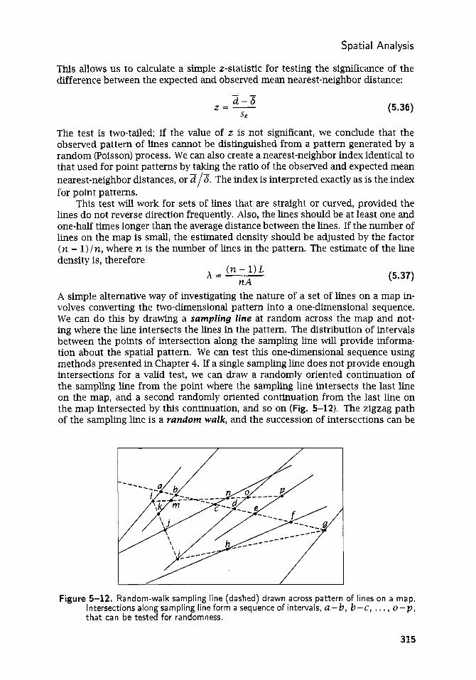
Spatial Analysis
This allows us to calculate a simple z-statistic for testing the significance of the difference between the expected and observed mean nearest-neighbor distance:
(5.36)
The test is two-tailed; if the value of z is not significant, we conclude that the observed pattern of lines cannot be distinguished from a pattern generated by a random (Poisson) process. We can also create a nearest-neighbor index identical to that used for point patterns by taking the ratio of the observed and expected mean nearest-neighbor distances, or d / 6 . The index is interpreted exactly as is the index for point patterns.
This test will work for sets of lines that are straight or curved, provided the lines do not reverse direction frequently. Also, the lines should be at least one and one-half times longer than the average distance between the lines. If the number of lines on the map is small, the estimated density should be adjusted by the factor (n - 1) In, where n is the number of lines in the pattern. The estimate of the line
- -
density is, therefore (n- l ) L
nA A = (5.37)
A simple alternative way of investigating the nature of a set of lines on a map in- volves converting the two-dimensional pattern into a one-dimensional sequence. We can do this by drawing a sampling line at random across the map and not- ing where the line intersects the lines in the pattern. The distribution of intervals between the points of intersection along the sampling line will provide informa- tion about the spatial pattern. We can test this one-dimensional sequence using methods presented in Chapter 4. If a single sampling line does not provide enough intersections for a valid test, we can draw a randomly oriented continuation of the sampling line from the point where the sampling line intersects the last line on the map, and a second randomly oriented continuation from the last line on the map intersected by this continuation, and so on (Fig. 5-12). The zigzag path of the sampling line is a random walk, and the succession of intersections can be
Figure 5-12. Random-walk sampling line (dashed) drawn across pattern of lines on a map. Intersections along sampling line form a sequence of intervals, a-b, b-c, , . , , o - p , that can be tested for randomness.
315

Statistics and Data Analysis in Geology - Chapter 5
treated as though they occurred along a single, straight sampling line. This and other methods for investigating the density of patterns of lines are reviewed by Getis and Boots (1978). A computer program for computing nearest-neighbor dis- tances, orientation, and other statistical measures of patterns of lines is given by Clark and Wilson (1994).
Analysis of Directional Da ta Directional data are an important category of geologic information. Bedding planes, fault surfaces, and joints are all characterized by their attitudes, expressed as strikes and dips. Glacial striations, sole marks, fossil shells, and water-laid peb- bles may have preferred orientations. Aerial and satellite photographs may show oriented linear patterns. These features can be measured and treated quantitatively like measurements of other geologic properties, but it is necessary to use special statistics that reflect the circular (or spherical) nature of directional data.
Following the practice of geographers, we can distinguish between directional and oriented features. Suppose a car is traveling north along a highway; the car’s motion has direction, while the highway itself has only a north-south orientation. Strikes of outcrops and the traces of faults are examples of geologic observations that are oriented, while drumlins and certain fossils such as high-spired gastropods have clear directional characteristics.
We may also distinguish observations that are distributed on a circle, such as paleocurrent measurements, and those that are distributed spherically, such as measurements of metamorphic fabric. The former data are conventionally shown as rose diagrams, a form of circular histogram, while the latter are plotted as points on a projection of a hemisphere. Although geologists have plotted direc- tional measurements in these forms for many years, they have not used formal statistical techniques extensively to test the veracity of the conclusions they have drawn from their diagrams. This is doubly unfortunate; not only are these statis- tical tests useful, but the development of many of the procedures was originally inspired by problems in the Earth sciences.
Figure 5-13 is a map of glacial striations measured in a small area of south- ern Finland; the measurements are listed in Table 5-4 and contained in file FIN- LAND.TXT. The directions indicated by the striations can be expressed by plotting them as unit vectors or on a circle of unit radius as in Figure 5-14 a. If the circle is subdivided into segments and the number of vectors within each segment counted, the results can be expressed as the rose diagram, or circular histogram, shown as Figure 5-14 b.
Nemec (1988) pointed out that many of the rose diagrams published by ge- ologists violate the basic principal on which histograms are based and, as a con- sequence, the diagrams are visually misleading. Recall that areas of columns in a histogram are proportional to the number (or percentage) of observations occurring in the corresponding intervals. For a rose diagram to correctly represent a circular distribution, it must be constructed so that the areas of the wedges (or “petals”) of the diagram are proportional to class frequencies. Unfortunately, most rose dia- grams are drawn so that the radii of the wedges are proportional to frequency. The resulting distortion may suggest the presence of a strong directional trend where none exists (Fig. 5-15).
316

Spatial Analysis
Figure 5-13. Map showing location and direction of 51 measurements of glacial striations in a 35-km2 area of southern Finland.
Table 5-4. Vector directions of glacial striations measured in an area of southern Finland; measure-
ments given in degrees clockwise from north.
23 105 127 144 171 27 113 127 145 172 53 113 128 145 179 58 114 128 146 181 64 117 129 153 186 83 121 132 155 190 85 123 132 155 212 88 125 132 155 93 126 134 157 99 126 135 163
100 126 137 165
If we define a radius for a sector of a rose diagram that represents either one observation, or 1%, we can easily calculate the appropriate radii that represent any number of observations or relative frequencies,
Yf = Yufi (5.38)
where r, is the unit radius representing one observation or 1%, f is the frequency (in counts or percent) of observations within a class, and yf is the radius of the class sector. In other words, the radius should be proportional to the square root of the frequency rather than to the frequency itself.
Rose diagrams, even if properly scaled, suffer from the same problems as or- dinary histograms; their appearance is extremely sensitive to the choice of class widths and starting point and they exhibit variations similar to the histogram
317

Statistics and Data Analysis in Geology - Chapter 5
Figure 5-14. Directions of glacial striations shown on Figure 5-13. (a) Directions plotted as unit vectors. (b ) Directions plotted as a rose diagram showing numbers of vectors within successive 10" segments.
Figure 5-15. Rose diagram o f glacial striations shown on Figure 5-13 plotted in 10" seg- ments. (a) Length of petals proportional t o frequency. (b ) Area of petals proportional t o frequency.
examples shownin Figure 2-11 onp. 30. Wells (1999) provides a computer program that quickly constructs rose diagrams with different conventions and also includes an assortment of graphical alternatives that may be superior to conventional rose diagrams for some uses (Fig. 5-16).
To compute statistics that describe characteristics of an entire set of vectors, we must work directly with the individual directional measurements rather than with a graphical summary such as a rose diagram. (Note that the following dis- cussion uses geological and geographic conventions in which angles are measured clockwise from north, or from the positive end of the Y-axis. Many papers on di- rectional statistics follow a mathematical convention in which angles are measured counterclockwise from east, or from the positive end of the X-axis.)
318

S patia I Analysis
Figure 5-16. Effect of choice of segment size and origin on appearance of rose diagrams. Data are directions of glacial striations from file FINLAND.TXT: (a) 5" segments, 0" origin, outer ring 20%; (b ) 15" segments, 0" origin, outer ring 30%; (c) 30" segments, 0" origin, outer ring 40%; ( d ) 15" segments, 10" origin-compare to (b ) . Alternative graphical forms include (e) kite diagram, 15" segments, 0" origin-sometimes used in statistical presentations; ( f ) circular histogram, 15" segments, 0" origin-widely used to plot wind directions.
The dominant direction in a set of vectors can be found by computing the vector resultant. The X- and Y-coordinates of the end point of a unit vector whose direction is given by the angle 8 are
xi = cos ei =s in& (5.39)
Three such vectors are shown plotted in Figure 5-17. Also shown is the vector resultant, R , obtained by summing the sines and cosines of the individual vectors:
(5.40)
From the resultant, we can obtain the mean direction, 3, which is the angular av- erage of all of the vectors in a sample. It is directly analogous to the mean value of a set of scalar measurements
(5.41)
Obviously, the magnitude or length of the resultant depends in part on the amount of dispersion in the sample of vectors, but it also depends upon the number of
319

Statistics and Data Analysis in Geology - Chapter 5
I R
U b
Figure 5-17. Determination of mean direction of a set of unit vectors. (a) Three vectors taken from Figure 5-16. (b ) Vector resultant, R , obtained by combining the three unit vectors. Order of combination is immaterial.
a b
Figure 5-18. Use of length of resultant to express dispersion in a collection of unit vectors. (a) Three vectors tightly clustered around a common direction. Resultant R is rela- tively long, approaching the value of n. (6) Three widely dispersed vectors; resultant length is less than 1.0.
vectors. In order to compare resultants from samples of different sizes, they must be converted into a standardized form. This is done simply by dividing the coordi- nates of the resultant by the number of observations, n
(5.42)
Note that these coordinates also define the centroid of the end points of the indi- vidual unit vectors.
'The resultant provides information not only about the average direction of a set of vectors, but also on the spread of the vectors about this average. Figure 5-18 a shows three vectors that deviate only slightly from the mean direction. The resultant is almost equal in length to the sum of the lengths of the three vectors. In contrast, three vectors in Figure 5-18 b are widely dispersed; their resultant is very short. The length of the resultant, R , is given by the Pythagorean theorem:
(5.43)
The length of the resultant can be standardized by dividing by the number of obser- vations. The standardized resultant length can also be found from the standardized end points
- R Jn (5.44) R = - = C + S n
320
Next Page

In previous chapters we have considered the analysis of data consisting of only a single variable measured on each specimen or observational unit. In Chapters 4 and 5 we also considered the influence of the temporal or geographic coordinates of the sample points. We will now examine techniques for the analysis of multivariate data, in which each observational unit is characterized by several variables. Multi- variate methods allow us to consider changes in several properties simultaneously. Examples of data appropriate for multivariate analysis abound in geology. They include chemical analyses, where the variables may be percentage compositions or parts per million of trace elements; measures on streams, such as discharge, suspended sediment load, depth, dissolved solids, pH, and oxygen content; and paleontologic variables, perhaps a large number of measurements made on speci- mens of an organism. Dozens of other examples quickly spring to mind. Some are simple extensions of problems we have considered previously; others are entirely new classes of problems.
Multivariate methods are extremely powerful, for they allow the researcher to manipulate more variables than can otherwise be assimilated. They are compli- cated, however, both in their theoretical structure and in their operational method- ology. For some of the procedures, statistical theory and tests have been worked out only for the most restrictive set of assumptions. The nature and behavior of the tests under more relaxed, general assumptions (such as those necessary for most real-world problems) are inadequately known. In fact, some of the procedures we will consider have no theoretical statistical basis at all, and tests of significance have yet to be devised. Nevertheless, these methods seem to hold the most promise for fruitful returns in geological investigations. Most of the problems in geology involve complex and interacting forces which are impossible to isolate and study individually. Often a meaningful decision as to the relative worth of one of a num- ber of possible variables cannot be made. The best course of action frequently is
Statistics and Data Analysis in Geology - Chapter 6
to examine as many facets of a problem as possible, and sort out, a posteriori, the major factors. The methods discussed in this chapter can be a significant help.
Multiple Regression The first topic we will consider in our final chapter is actually a familiar subject under a new and more general guise. This is multiple regression, which includes polynomial curve fitting (discussed in Chapter 4) and trend-surface analysis (dis- cussed in Chapter 5). However, we will now remove the restrictions that limited us to considerations of change as a function of temporal or spatial coordinates. Any observed variable can be considered to be a function of any other variable measured on the same samples. In Chapter 4 we considered changes in moisture content that occurred with changes in depth in the sediment. We could equally well have measured the montmorillonite content of the sediment in the core and examined the changes in water content that may accompany changes in montmo- rillonite percentage. In fact we could have measured several variables, perhaps organic content, mean grain size, and bulk density, and we could have examined the differences in water content associated with changes in each or all of these variables. In a sense, variables may be considered as dimensions, and their values as coordinates, so we can envision changes occurring “along” a dimension defined by a variable such as mineral content. Casting variables as dimensions is nothing new; we perform this every time we plot two variables against one another, because we are substituting spatial scales in the plot for the original scales on which the variables were measured. Such interchangeability is explicit in the references to “ p - dimensional space” which abound in the literature of multivariate analysis. Just as trend surfaces are a generalization of curve-fitting procedures to two-dimensional space, multiple regression is a further generalization to “many-dimensional” space.
We will not consider multiple regression in great detail because the theoretical and computational essentials have been presented in earlier chapters. You will re- call from Chapter 4 that polynomial regressions (having one independent variable) can be represented in a model equation of the general form
The model states that the value of a dependent variable, yi, at a location i is equal to a constant term plus the sum of a series of powers of an independent variable, xli, also observed at location i, plus a random error that is unique for location i. A least-squares solution to a linear equation of this type can be found by solving a set of normal equations for the P coefficients. These can be expressed in matrix form as
S x y = S = b (6.2) with a solution
b=S&Sxy
where S X ~ is a column matrix of the sums of cross products of y, with xl, xf, . . . , x y ; SXX is a matrix of sums of squares and cross products of the X I , x:, . . . , x? powers; and b estimates 8, the column matrix of unknown regression coefficients. In Chapter 4, we found the entries in the various matrices by labeling rows and columns and cross multiplying.
462

Analysis of Multivariate Data
Although we regarded this problem as involving only one independent variable (or two, in the case of trend-surface analysis as discussed in Chapter 5), it can be regarded as containing m independent variables. This can readily be seen if we rewrite the model equation as
yi = /30 + BlXl i + /3ZXZi + - * ‘ + /3mxmi + E i (6.4)
and define the variables as x1 = XI, xg = x:, x 3 = x:, and so forth. Thus, the regression procedures we have considered up to this point have simply involved the definition of the independent variables in a specific manner.
A regression of any m independent variables upon a dependent variable can be expressed as in Equation (6.4). The normal equations that will yield a least-squares solution can be found by appropriate labeling of the rows and columns of the matrix equation and cross multiplying to find the entries in the body of the matrix. For three independent variables, we obtain
where, again, xo is a dummy variable equal to 1 for every observation. The matrix equation, after cross multiplication, is
The 6’s in the regression model are estimated by the b’s, the sample partial regression coefficients. They are called partial regression coefficients because each gives the rate of change (or slope) in the dependent variable for a unit change in that particular independent variable, provided all other independent variables are held constant. Some statistics books emphasize this point by using the notation
The coefficient b1.23, for example, is read “the regression coefficient of variable x1 on y as variables xg and x 3 remain constant.” In general, these coefficients will differ from the total regression coefficients, which are the simple regressions of each individual x variable on the dependent y variable. We ordinarily expect multiple regression coefficients to account for more of the total variation in y than will any of the total regression coefficients. This is because multiple regression considers all possible interactions within combinations of variables as well as the variables themselves.
We will consider a problem in geomorphology to illustrate a typical application of multiple regression. For this study, a well-dissected area of relatively homoge- neous geology was selected in eastern Kentucky. The study region contains many drainage basins of differing sizes; from these, all third-order basins were chosen,
463

Statistics and Data Analysis in Geology - Chapter 6
and several variables were measured on each. The order of a drainage basin is defined by the number of successive levels of junctions on its stream from the stream’s sources to the point where it joins another stream of equal or higher or- der. Thus, a third-order basin has two levels of junctions within its boundaries. Basin size, however, may be defined by many alternative methods. One of these is basin magnitude, which essentially is a count of the number of sources in the basin. A collection of basins of specified order may contain many different mag- nitudes. The relationship between magnitude and order of streams in drainage basins is shown in Figure 6-1. Seven variables were measured on the collection of third-order basins:
Y - x1 - XZ - x3 - x4 - xs - x6 -
Basin magnitude, defined by the number of sources. Elevation of the basin outlet, in feet. Relief of the basin, in feet. Basin area, in square miles. Total length of the stream in the basin, in miles. Drainage density, defined as total length of stream in basinbasin area. Basin shape, measured as the ratio of inscribed to circumscribed circles.
1 Y 2
a b C
Figure 6-1. Contrast between stream magnitude and stream order. (a ) Tenth-magnitude stream of second order. (b ) Tenth-magnitude stream of third order. (c) Fourth- magnitude stream of third order. Magnitude is based on number of joining streams; order is based on succession of joining.
Our problem is to determine the influence of the six independent X variables on variable Y . Multiple regression, using basin magnitude as the dependent vari- able, is an appropriate technique. From the regression, the influence that all the variables have on basin magnitude can be assessed. File KENTUCKY.TXT contains measurements on these variables for 50 third-order basins in eastern Kentucky, taken from Krumbein and Shreve (1970). The significance of the linear relationship can be tested by analysis-of-variance methods presented in Chapter 4. Table 4-9 (p. 197), for example, outlines the ANOVA for simple linear regression which may be expanded to multiple regression by changing the various degrees of freedom to account for additional variables. The modified ANOVA is shown in Table 6-1. The
464

Analysis of Multivariate Data
Table 6-1. ANOVA for multiple regression with m independent variables.
Source of Variation
Linear Regression
Deviation
Total Variation
Variation Squares F-Test
Linear MSR I MSD
Sum of Degrees of Mean Squares Freedom Squares F-Test
1800.70 6 300.12 11.38**
43 26.38 34.
2934.82 49
t I I I I I
Table 6-2. Completed ANOVA for the significance o f regression o f six geomorphic variables on basin magnitude.'
completed ANOVA for multiple regression on basin magnitude is shown in Table 6-2. The regression coefficients are also shown.
In multiple-regression problems, we usually are interested in the relative ef- fectiveness of the independent variables as predictors of the dependent variable. We cannot determine this from a direct examination of the regression coefficients, however, because their magnitudes are dependent upon the magnitudes of the vari- ables themselves, which in part reflect the units of measurement. This is apparent in trend-surface analysis, where coefficients of higher orders almost invariably de- crease in absolute size, even though higher orders may make greater contributions to the trend than lower orders. This results from the fact that a geographic coordi- nate, raised to a power as it is in high orders, is much larger in magnitude than the original coordinate. The higher order regression coefficients become correspond- ingly smaller.
Fortunately, it is easy to standardize the partial regression coefficients by con- verting them to units of standard deviation. The standard partial regression coef- ficients, &, are found by
(6.6) sk Bk = bk- SY
where Sk is the standard deviation of variable xk and sy is the standard deviation of y. Because the standard partial regression coefficients are all expressed in units
465

Statistics and Data Analysis in Geology - Chapter 6
of standard deviation, they may be compared directly with each other to determine the most effective variables.
To compute the matrix of sums of squares and products necessary in the nor- mal equation set, we found the diagonal entries, C x i . It is a simple matter to convert these sums of squares to corrected sums of squares, ssk, and then to the standard deviations necessary to compute the partial correlation coefficients. However, it is possible to solve the normal equations in a manner that will yield the standardized partial regression coefficients directly, and gain an important com- putational advantage in the process.
The major sources of error in multiple regression occur in the creation of the entries in the S n matrix and during the inversion process. The sums of squares of the variables may become so large that significant digits are lost by truncation. If the entries in the S n matrix differ greatly in their magnitudes, an additional loss of digits may occur during inversion, especially if high correlations exist among the variables. Some computer programs may be capable of retaining only one or two significant digits in the coefficients, and with certain data sets retention may even be worse. Studies have shown that calculations using double-precision arithmetic may not be sufficient to overcome this problem. However, a few simple modifi- cations in our computational procedure will gain us two to six significant digits during computation and greatly increase the accuracy of the computed regression (Longley, 1967, p. 821-827).
The most obvious step that can be taken is to convert all observations to devia- tions from the mean. This reduces the absolute magnitude of variables and centers them about a common mean of zero. As an inevitable consequence, the coefficient bo will become zero, so the matrix equation can be reduced by one row and one column. This simple step may gain several significant digits. However, we also may reduce the size of entries in the matrix still further by converting them all to correlations. This is equivalent to expressing the original variables in the standard normal form of zero mean and unit standard deviation. The matrix equation for regression then has the form
R m B = R x y
which can be solved by the operation
B = R & R ~ (6.8)
where R w represents the column vector of correlations between y and the xk independent variables. The m x m matrix of correlations between the xk variables is represented by RXX. For example, the normal equation for three independent variables has the form
Note that the equation has one less row and column than the equivalent equation using the original variables (Eq. 6.5).
Computing the regression equation in standardized form has the disadvantage that the correlation matrix must be created first, increasing the computational ef- fort. In order to preserve accuracy, the correlations must be calculated using the
466

Analysis of Multivariate Data
definitional equation for the sums of products (Eq. 2.23; p. 40) rather than with the computational form for correlation given in Equation (2.28). This is because Equa- tion (2.28) involves squaring the quantities C x; and C x:. If these sums are large, the squares may be inaccurate because of truncation. This problem is avoided if the means are subtracted from each observation prior to calculation of the sums of squares. The sums of squares are then found by Equations (2.19) and (2.23). This process requires that the data be handled twice-first to calculate the means, and then to subtract out this quantity during calculations. Although this involves a significant increase in labor if computations are performed by hand, the additional effort is trivial on a digital computer. Also, the resulting coefficients must be “un- standardized” if they are to be used in a predictive equation with raw data. However, these disadvantages are more than offset by the increased stability and accuracy of the matrix solution, and the standardized coefficients provide a way of assessing the importance of individual variables in the regression. Partial regression coeffi- cients can be derived from the standardized partial regression coefficients by the transformation
(6.10) SY bk = Bk- s k
The constant term, b o , can be found by
(6.11)
Although the various sums of squares change if the data are standardized (i.e., the correlation form of the matrix equation is used), the ratios of the sums of squares remain the same. Therefore, tests of significance based on standardized regression are identical to those based on an unstandardized regression. Quantities such as the coefficient of multiple correlation (R) and percentage of goodness of fit (100% R 2 ) also remain unchanged.
We can compare the partial regression coefficients between basin magnitude and the other six basin properties in both raw and standardized form:
b‘ = [ -2.244 0.005 0.226 -0.233 0.063 -0.002 -0.1171
B’ = [ 0.000 0.049 0.284 -0.458 0.975 -0.120 -0.1631
Although the standardized partial regression coefficients suggest that the basin properties having the most pronounced relationship with basin magnitude are x2 (relief), x3 (area), and x4 (stream length), these values do not take into ac- count the uncertainty associated with each estimated parameter. The easiest way to consider this aspect is by expanding the analysis of variance to test the significance of each independent variable.
The sum of squares attributable to a single variable, X j , can be determined by calculating SSR(,) for the regression with all m variables, calculating S S R ( , - ~ ) , which is the sum of squares for regression using all variables except the j t h variable, then finding the difference. This process can be repeated for each independent variable in turn, in order to assess the contribution that each makes to the total regression. Fortunately, there is an easier way to calculate the individual regres- sion sums of squares, which simply requires dividing the square of each partial regression coefficient by the diagonal elements of S& that correspond to each of the variables. If we designate CXX = S&, then
(6.12)
467

Statistics and Data Analysis in Geology- Chapter 6
Once the regression sums of squares of the individual variables have been calculated, they can be entered into an expanded ANOVA table such as that shown in Table 6-3 and tested for significance. The F-test ratios are formed from the mean squares due to partial regression with each of the individual variables in the numerators, and the mean square due to deviation from the regression model as the denominator. Each F-test has 1 and (n - m - 1) associated degrees of freedom. The F-tests will not change if the calculations are based on standardized partial regression coefficients.
Table 6-3. ANOVA for testing the significance of partial regression of individual variables.
A complete ANOVA for testing the significance of the partial regression of each geomorphic variable on basin magnitude is given in Table 6-4. Although basin relief, basin area, and stream length all have the largest standardized partial regression coefficients, the contribution to the total regression made by basin area is not statistically significant. This is because the partial regression coefficient for basin area has an associated high standard error.
Although the standardized partial regression coefficients provide a guide to the most effective variables in the regression, they are not an infallible index to the “best possible’’ regression equation. Suppose you examine the regression equation and decide two variables are contributing a negligible amount to the regression and can be discarded. When one of the variables is omitted and the regression is recal- culated, the goodness of fit and the regression equation, of course, change. Now suppose you decide to discard the second variable; again the regression changes. But the change might be quite different from the change that would occur if the first discarded variable were still in the regression. This occurs because the interac- tion effects of the two discarded variables with other variables cannot be assessed without recomputing the regression. If we want to search through a large set of variables and “weed out” those which are not helpful in the problem, we must do more than simply examine the partial regression coefficients.
468

Analysis of Multivariate Data
Deviation
Total Variation
1134.12 43 26.38
2934.82 49
Increasing the number of independent variables in the regression equation will always increase the SSR (except in the situation where a new variable is perfectly correlated with a previous variable). However, the increase may not be significant. The loss of degrees of freedom for deviations may offset the reduction in SSD, and actually increase the mean squares due to deviation. If this happens, the F-ratio for the significance of the regression will decrease, and the addition of another variable has actually detracted from the regression. To determine the very best possible regression (in the sense of having the most significant F-ratio), all possible combinations of the variables would have to be examined. This is possible if we are dealing with few variables, but the number of possible variable combinations is equal to 2m - 1, and the computational effort is formidable if m is large. Other procedures are available which yield a nearly optimal regression with much less effort. These include schemes such as the backward elimination procedure, the forward selection procedure, stepwise regression, and stagewise regression. These methods may not find identical regression equations in a large selection of possible variables, but all will produce approximately equivalent results. A consideration of each is beyond the scope of this book; we will be content with a brief description
469

Statistics and Data Analysis in Geology - Chapter 6
of one of the techniques. These methods are well described in some of the texts listed in the Selected Readings at the end of the chapter, especially in Marascuilo and Levin (1983) and in Draper and Smith (1998).
The backward elimination procedure consists of computing a regression in- cluding all possible variables and selecting the least significant variable. The selec- tion proceeds by examining the standardized partial regression coefficients for the smallest value and then recomputing the regression, omitting that variable. The significance of the deleted variable is tested by the analysis of variance shown in Table 6-3. If the variable is not making a significant contribution to the regres- sion, it is permanently discarded. The reduced regression model is then fitted to the data, a new set of standardized partial regression coefficients for the reduced equation is calculated, and the process is repeated. At each step, the regression equation is reduced by one variable, until all remaining variables are significant.
It is instructive to examine the collection of six independent variables mea- sured on river basins (file KENTUCKY.TXT) and see if any can be discarded without significantly affecting the multiple regression on basin magnitude. We can find a minimal set of regressions by examining the standardized partial regression coeffi- cients, deleting the smallest of these, and recomputing the regression. Repeatedly running a multiple-regression program obviously is less efficient than using a step- wise computer program, but it has the advantage that every step in the process can be examined closely. When you are confident that you understand the elimination process and the changes that occur in the regression coefficients, you may turn to a more automated procedure.
Although multiple regression is “multivariate” in the sense that more than one variable is measured on each observational unit, it really is a univariate technique because we are concerned only with the variance of one variable, y . Behavior of the independent variables, the x’s, is not subject to analysis.
The next topic we will consider is discriminant function analysis, which in- volves identification or the placing of objects into predefined groups. The discrim- ination between two alternative groups is a process that is computationally inter- mediate between univariate procedures and true multivariate methods in which many variables are considered simultaneously. Two groups, each characterized by a set of multiple variables, can be discriminated by solving a set of simultaneous equations almost identical to those involved in multiple regression. The right-hand vector of the matrix equation, however, does not contain cross products between independent variables and a single dependent variable, but rather differences be- tween the multivariate means of the two groups that are to be discriminated.
Tests of discriminant functions involve multivariate extensions of simple uni- variate statistical tests of equality. These will be considered next, followed by a dis- cussion of multivariate classification, or the sorting of objects into homogeneous groups. We will then consider eigenvector techniques, including principal compo- nent and factor analysis. The final topics will include multivariate extensions of discriminant analysis and multiple regression.
This list of topics is certainly not all-inclusive. However, the subjects have been chosen because they have found special utility in the Earth sciences. They include a wide variety of computational techniques and encompass many fundamental con- cepts. An understanding of the theory and operational procedures involved in these methods should provide you with a sufficient background to evaluate other multivariate techniques as well.
470

Analysis of Multivariate Data
Discri m i na nt Functions One of the most widely used multivariate procedures in Earth science is the dis- criminant function. We will consider it at length for two reasons: discrimination is a powerful statistical tool and it can be regarded as either a way to treat univariate problems related to multiple regression, ‘or multivariate problems related to the statistical tests we will discuss later. Discriminant functions therefore provide an additional link between univariate and multivariate statistics.
First, however, we must define the process of discrimination, and carefully distinguish it from the related process of classification. Suppose we have assembled two collections of shale samples of known freshwater and saltwater origin. We may have determined their origin from an examination of their fossil content. A number of geochemical variables have been measured on each specimen, including the content of vanadium, boron, iron, and so forth. The problem is to find the linear combination of these variables that produces the maximum difference between the two previously defined groups. If we find a function that produces a significant difference, we can use it to allocate new specimens of shale of unknown origin to one of the two original groups. In other words, new shale samples, not containing diagnostic fossils, can then be categorized as marine or freshwater on the basis of the linear discriminant function of their geochemical components. [This problem was considered by Potter, Shimp, and Witters (1963).]
Classification can be illustrated with a similar example. Suppose we have ob- tained a large, heterogeneous collection of shale specimens, each of which has been geochemically analyzed. On the basis of the measured variables, can the shales be separated into groups (or clusters, as they are commonly called) that are both rel- atively homogeneous and distinct from other groups? The process by which this can be done has been highly developed by numerical taxonomists, and will be con- sidered in a later section. There are several obvious differences between these pro- cedures and those of discriminant function analysis. A classification is internally based; that is, it does not depend on a priori knowledge about relations between observations as does a discriminant function. The number of groups in a discrim- inant function is set prior to the analysis, while in contrast the number of clusters that will emerge from a classification scheme cannot ordinarily be predetermined. Similarly, each original observation is defined as belonging to a specific group in a discriminant analysis. In most classification procedures, an observation is free to enter any cluster that emerges. Other differences will become apparent as we examine these two procedures. The result of a cluster analysis of shales would be a classification of the observations into several groups. It would then be up to us to interpret the geological meaning (if any) of the groups so found.
A simple linear discriminant function transforms an original set of measure- ments on a specimen into a single discriminant score. That score, or transformed variable, represents the specimen’s position along a line defined by the linear dis- criminant function. We can therefore think of the discriminant function as a way of collapsing a multivariate problem down into a problem which involves only one variable.
Discriminant function analysis consists of finding a transform which gives the maximum ratio of the difference between two group multivariate means to the multivariate variance within the two groups. If we regard our two groups as form- ing clusters of points in multivariate space, we must search for the one orienta- tion along which the two clusters have the greatest separation while each cluster
471

Statistics and Data Analysis in Geology- Chapter 6
simultaneously has the least inflation. This can be graphically shown for two- dimensional cases, as in Figure 6-2, which is a scatter plot of the two groups of data listed in file SANDS.TXT. One group contains grain-size statistics of modern beach sands collected along the Gulf Coast in Texas; the second group contains grain-size statistics for sands collected offshore in the Gulf of Mexico. Both data sets consist of two variables, the median grain size and the grain-size sorting coefficient. Al- though the two clusters of points overlap, it is apparent that a line of division could be placed between the two clusters such that most of the beach sands would be on one side and most offshore sands would be on the other. An adequate separation between the sands of the two groups cannot be made using either median grain size or sorting coefficient alone. However, it is possible to find the orientation of an axis along which the two sets of sands are separated the most and inflated the least. The coordinates of this axis are the coefficients of the linear discriminant function.
Figure 6-2. Plot of distributions of median grain size and sorting coefFicient for samples of modern sands, with scatter plot of both variables. Samples indicated by open circles are beach sands, those indicated by solid dots are ofkhore sands. Dashed lines indicate bivariate means of the two groups. Distribution of discriminant scores also is shown along line parallel t o discriminant axis.
One method that can be used to find the discriminant function is regres- sion; however, the dependent variable consists of the differences between the
472

Analysis of Multivariate Data
multivariate means of the two groups. In matrix notation, we must solve an equa- tion of the form
SA = D (6.13)
where S is an m x m matrix of pooled variances and covariances of the m variables. The coefficients of the discriminant equation are represented by a column vector of the unknown lambdas. Lowercase lambdas (A) are used by convention to represent the coefficients of the discriminant function. These are exactly the same as the betas (p ) used (also by convention) in regression equations. They should not be confused with lambdas used to represent eigenvalues in principal component or factor analyses.
The right-hand side of the equation consists of the column vector of m differ- ences between the means of the two groups, which we will refer to as A and B. You will recall from Chapter 3 that such an equation can be solved by inversion and multiplication, as
A = S-lD (6.14)
where S-' is the inverse of the variance-covariance matrix formed by pooling the matrices of the sums of squares and cross products of the two groups, A and B. To compute the discriminant function, we must determine the various entries in the matrix equation. The mean differences are found simply by
(6.15)
In this notation, a i j is the i t h observation on variable j in group A and Z j is the mean of variable j in group A, which is the arithmetic average of the na observations of variable j in group A. The same conventions apply to group B . The multivariate means of groups A and B can be regarded as forming two vectors. The difference between these multivariate means therefore also forms a vector
D = A - B
or, in expanded form,
To construct the matrix of pooled variances and covariances, we must compute a matrix of sums of squares and cross products of all variables in group A and a similar matrix for group B . For example, considering only group A,
Here, U i j denotes the i t h observation of variable j in group A as before, and d.ik denotes the i t h Observation of variable k in the same group. Of course, this quantity will be the sum of squares of variable k whenever j = k. Similarly, a matrix of sums of squares and cross products can be found for group B:
473

Statistics and Data Analysis in Geology - Chapter 6
Table 6-5. Matrices necessary to compute discriminant function between beach sands and ofFshore sands listed in file SANDS-TXT.
Vector mean of beach sands:
Vector mean of offshore sands:
Vector of mean differences:
Corrected sums of squares for beach sands:
Corrected sums of squares for offshore sands:
Pooled variance- covariance matrix:
Inverse of pooled variance- covariance matrix:
[ 0.3297 1.16741
[ 0.3399 1.21001
[ -0.0101 -0.04261
0.000925 -0.004886 -0.004886 0.075662
0.001384 -0.008440 -0.008440 0.107000
1 0.000029 -0.000687 -0.000687 0.002312
1 59,098.3047 4311.6403 4311.6403 747.0581
We will denote the sums of products matrix from group A as SA and that from group B as S B . The matrix of pooled variance can now be found as
S A f S B S = n, + n b - 2 (6.16)
Remember this equation for the pooled variance: we will use it later in a T 2 test of the equality of the multivariate means of the two groups. Although the amount of mathematical manipulation that must be performed to calculate the coefficients of a discriminant function appears large, it actually is less formidable than it seems at first glance. To demonstrate, we can calculate a discriminant function between the two groups of observations in file SANDS.TXT. Group A consists of the beach sands and Group B consists of the offshore sands.
Table 6-5 contains the calculations necessary to find the two vectors of mul- tivariate means and the two matrices of sums of squares and products. From these, the matrix of pooled variances is calculated. We now have all of the entries
474

Analysis of Multivariate Data
necessary to estimate the discriminant function coefficients:
S D h - 783.442 ] ’ [ 1::::!] = [ -75.602 ] 59,098.305 4311.640
4311.640 747.058 [ The set of h coefficients we have found are entries in the discriminant function equation which has the form
Equation (6.17) is a linear function; that is, all the terms are added together to yield a single number, the discriminant score, Ri. In a two-dimensional example, we can plot the discriminant function as a line on the scatter diagram of the two original variables. It is a line through the plot whose slope, a, is
a = h2Ihl (6.18)
Substitution of the midpoint between the two group means into the discriminant function equation yields the discriminant index, Ro. That is, for each value of Xji in Equation (6.17), we insert the terms
- A j + B j
X j . = - 2 (6.19)
In our example,
Ro = (-783.442 * 0.335) + (-75.602 . 1.189) = -352.146
The discriminant index, Ro, is the point along the discriminant function line that is exactly halfway between the center of group A and the center of group B. Next, we may substitute the multivariate mean of group A into the equation (that is, we set X j :Xj) to obtain RA and substitute the multivariate mean of group B (setting X j = Bj) to obtain RB. The centers of the two original groups projected onto the axis defined by the discriminant function are RA and RB.
For group A,
RA = (-783.442 . 0.330) + (-75.602 * 1.167) = -346.560
and for group B,
RB = (-783.442 * 0.340) + (-75.602 . 1.210) = -357.732
The three points may be plotted as in Figure 6-3. In fact, every observation in the analysis can be entered into the equation and its position along the discrim- inant function located. These values are the raw discriminant scores. This has been done on Figure 6-3; note that a few members of group A are located on the
475

Statistics and Data Analysis in Geology - Chapter 6
I I I
1 1 ' 1 1 1 1 ' 1 ~ 1 1 ~ ~ 1 1 1 1 1 1 1 1 1 ~ ~ 1 ~ ~ 1 ~ 1 -335 -340 -345 -350 -355 -360 -365
Raw discriminant scores
Figure 6-3. Projection of beach and offshore sands onto discriminant function line shown in Figure 6-2. RA is projection of bivariate mean of beach sands, RB is projection of bivariate mean of ofkhore sands, and Ro is discriminant index.
group B side of Ro and a few members of group B are located on the group A side. These are observations that have been misclassified by the discriminant func- tion. The misclassification ratio, or percent of observations that the discriminant function places into the wrong group, is sometimes taken as an indication of the function's discriminatory power. However, the misclassification ratio is biased and can be misleading because it is calculated by reusing the observations that were used to estimate the coefficients of the discriminant function in the first place. It seems likely that the function may be less successful in correctly classifying new observations. Reyment and Savazzi (1999) discuss alternative ways of evaluating the goodness of a discriminant function.
We have calculated the YUW discriminant function which yields raw scores whose units are products of the units of measurement attached to the original vari- ables. There actually are an infinity of discriminant functions that will maximize the difference between the two groups, but all of these alternatives are propor- tional to the classical, or raw, solution. If A is the vector of coefficients determined by Equation (6.14), then all sets cA (where c is an arbitrary constant), will serve equally well. Although different computer programs may yield sets of coefficients that seem to be different, all of them are proportional to each other. Alternative choices include:
1. The raw coefficients are divided by the pooled mean squares within groups, or
where c = MSK'
MSw = A ' S A
This standardizes the coefficients to dimensionless z-scores.
coefficient by the first coefficient, which becomes equal to 1.
raw coefficients. or
2. The raw coefficients are first divided by M S w , then rescaled by dividing every
3. Each raw coefficient is divided by the square root of the sum of the squared
The sum of the squares of the transformed coefficients will then be equal to 1.
476

Analysis of Multivariate Data
Tests of significance If we are willing to make some assumptions about the nature of the data used in the discriminant function, we can test the significance of the separation between the two groups. Five basic assumptions about the data are necessary: (a) the ob- servations in each group are randomly chosen, (b) the probability of an unknown observation belonging to either group is equal, (c) variables are normally distributed within each group, (d) the variance-covariance matrices of the groups are equal in size, and (e) none of the observations used to calculate the function were misclas- sified. Of these, the most difficult to justify are (b), (c), and (d). Fortunately, the discriminant function is not seriously affected by limited departures from normal- ity or by limited inequality of variances. Justification of (b) must depend upon a priori assessment of the relative abundance of the groups under examination. If the assumption of equal abundance seems unjustified, a different assumption may be made, which will shift the position of Ro. [See Anderson (1984, chapter 6) for an extensive discussion of alternative decision rules for discrimination.]
The first step in a test of the significance of a discriminant function is to mea- sure the separation or distinctness of the two groups. This can be done by comput- ing the distance between the centroids, or multivariate means, of the groups. The measure of distance is derived directly from univariate statistics. We can obtain a measure of the difference between the means of two univariate samples, XI and X z , by simply subtracting one from the other. However, this difference is expressed in the same units as the original observations. If the difference is divided by the pooled standard deviation, we obtain a standardized difference in which the dif- ference between the means of the two groups is expressed in dimensionless units of standard deviation, or z-scores:
J P
When both sides of Equation (6.20) are squared, variance of the two samples, s; :
(6.20)
the denominator is the pooled
(6.21)
Suppose that instead of a single variable, two variables are measured on each observation in the two groups. The difference between the bivariate means of the two groups can be expressed as the ordinary Euclidean, or straight-line, distance between them. Again denoting the two groups as A and B ,
Euclidean distance = J(X1 -El)' + (& - 8')' (6.22)
In general, if m variables are measured on each observation, the straight-line distance between the multivariate means of the two groups is
Euclidean distance = (Xj -Bj)' (6.23)
The square of the Euclidean distance is Cj"=, (Xj - Ej) ; you can verify that this is the same as the matrix product,
Euclidean distance' = D'D (6.24)
477
2

Statistics and Data Analysis in Geology - Chapter 6
The Euclidean distance and its square, unfortunately, are expressed as hodge- podges of the original units of measurement. To be interpretable, they must be standardized. Comparison with Equation (6.20) suggests that standardization must involve division by the multivariate equivalent of the variance, which is the variance-covariance matrix S. Of course, division is not a defined operation in ma- trix algebra, but we can accomplish the same end by multiplying by the inverse. Multiplying Equation (6.24) by the inverse of the variance-covariance matrix yields the standardized squared distance,
D2 = D‘ S-l D (6.25)
This standardized measure of difference between the means of two multivariate groups is called Mahalanobis’ distance. Substituting quantities from Table 6-5 into Equation (6.25), we obtain
59,098.305 4311.640 -0.010 D2 = [-0*010 -0.0431 [ 4311.640 747.0581 [ -0.0431
= 11.172
Interestingly, we can obtain exactly the same distance measure by substituting the vector of mean differences into the discriminant function equation itself
1 - 783.442 D 2 = [ -0.010 -0.0431 [ -75.602
= 11.172
Mahalanobis’ distance can be visualized on Figure 6-3, where it is equal to the distance between R A and RB.
The significance of Mahalanobis’ distance can be tested using a multivariate equivalent of the t-test of the equality of two means, called Hotelling’s T 2 test. We will discuss this test more extensively in the next section. Here, we simply note
(6.26) that it has the form
and can be transformed to an F-test. The test of multivariate equality, using this more familiar statistic, is
n a n b D 2 T 2 = n a + n b
) ( nanb ) D 2 na + n b
n, + n b - m - 1 F = ( (na + n b - 2) m (6.27)
with m and (na + nb - m - 1) degrees of freedom. The null hypothesis tested by this statistic is that the two multivariate means are equal, or that the distance between them is zero. That is,
against Ho: D = O
Hi: D > O
The appropriateness of this as a test of a discriminant function should be apparent. If the means of the two groups are very close together, it will be difficult to tell them apart, especially if both groups have large variances. In contrast, if the two means are well separated and scatter about the means is small, discrimination will
478

Analysis of Multivariate Data
be relatively easy. As an exercise, it may be instructive to calculate the significance of the discriminant function for the example we have just worked.
Not all of the variables we have included in the discriminant function will be equally useful in distinguishing one group from another. We may wish to iso- late those variables that are not especially helpful and eliminate them from future analyses. Selecting the most effective set of discriminators for discriminant func- tion analysis would seem to be analogous to selecting the most efficient predictors in multiple regression. The problem, however, is more complicated because the “dependent” or predicted variable in a discriminant function is composed of dif- ferences between two sets of the same variables that are used as “independent” predictors of the discrimination. Unlike regression, where the sums of squares of y do not change as different variables X j are added to the equation, the sums of squares of the differences between groups A and B do change as variables are added or deleted.
Some idea of the effectiveness of the variables as discriminators can be gained by computing the standardized differences,
(6.28)
This is simply the difference between the means of the two groups A and B for variable j , divided by the pooled standard deviation of variable j . Since the mea- sure does not consider interactions between variables, it is useful only as a general guide to discriminating power. Stepwise discriminant analysis programs may use standardized differences in choosing the order in which variables are added to the discriminant function. Marascuilo and Levin (1983) discuss “after-the-fact” con- trast procedures that can be used to select the most important variables. However, the significance of different combinations of variables can be tested only by com- puting the various functions and determining the relative amounts of separation the different equations produce between the two groups. To avoid bias, such tests should be run on independent random samples.
Discriminant function analysis provides a natural transition between two major classes of multivariate statistical techniques. On one hand, it is closely related to multiple regression and trend-surface analysis. On the other, it can be expressed as an eigenvalue problem, related to principal component analysis, factor analysis, and similar multivariate methods. There are advantages to the use of eigenvectors in calculating the discriminant function, because they allow us to simultaneously discriminate between more than two groups. However, we will delay a consideration of this topic until we examine the basic elements of eigenvector analysis and some of the simpler eigenvector techniques.
Multivariate Extensions of Elementary Statistics In Chapter 2, we considered some simple geologic problems that could be examined by elementary statistical methods. We will begin our consideration of multivariate methods in geology with some direct extensions of these simple tests. You will recall that the variation measured in most naturally occurring phenomena could be described by the normal distribution. This is a reflection of the central limit theo- rem, which states that observations which are the sums of many independently op- erating processes tend to be normally distributed as the number of effects becomes
479

Statistics and Data Analysis in Geology - Chapter 6
large. It is this tendency that allows us to use the normal probability distribution as a basis for statistical tests and provides the starting point for the development of the t - , F- , and x 2 distributions and others. The concept of the normal distribution can be extended to include situations in which observational units consist of many variables.
Suppose we collect rocks from an area and measure a set of properties on each specimen. The measurements may include determinations of chemical or miner- alogical constituents, specific gravity, magnetic susceptibility, radioactivity, or any of an almost endless list of possible variables. We can regard the set of measure- ments made on an individual rock as defining a vector Xi = [ xli x ~ i s - - xmi ], where there are m measured characteristics or variables. If a sample of observa- tions, each represented by vectors Xi, is randomly selected from a population that is the result of many independently acting processes, the observed vectors will tend to be multivariate normally distributed. Considered individually, each variate is normally distributed and characterized by a mean, pj , and a variance, uj. The joint probabizity distribution is a p-dimensional equivalent of the normal distribu- tion, having a vector mean p = [ p1 pz - . . pm ] and a variance generalized into the form of a diagonal matrix:
u; 0 * - .
. .
1 0 0 ::.. a& : 1 In addition to these obvious extensions of the normal distribution to the multivari- ate case, the multivariate normal distribution has an important additional charac- teristic. This is the covariance, covjk, which occupies all of the off-diagonal posi- tions of the matrixX. Thus, in the multivariate normal distribution, the mean is gen eralized into a vector and the variance into a matrix of variances and covariances. In the simple case of m = 2, the probability distribution forms a three-dimensional bell curve such as that in Figure 2-19, shown as a contour map in Figure 6-4. Al- though the distributions of variables x1 and x2 are shown along their respective axes, the essential characteristics of the joint probability distribution are better shown by the major and minor axes of the probability density ellipsoid. Many of the multivariate procedures we will discuss are concerned with the relative orien- tations of these major and minor axes.
One of the simplest tests we considered in Chapter 2 was a t-test of the prob- ability that a random sample of n observations had been drawn from a normal population with a specified mean, p, and an unknown variance, u2. The test, given in Equation (2.45) on p. 70, can be rewritten in the form
(6.29)
An obvious generalization of this test to the multivariate case is the substitu- tion of a vector of sample means for x, a vector of population means for p, and a variance-covariance matrix for s2. We have defined the vector of population means as p, so a vector of sample means can be designated X. Similarly, Z is the ma- trix of population variances and covariances, so S represents the matrix of sample variances and covariances. Both X and p are taken to be column vectors, although equivalent equations may be written in which they are assumed to be row vectors. A column vector of differences between the sample means and the population means
480

Analysis of Multivariate Data
-3 I I I I I I I I I I I -5 -4 -3 -2 - 1 0 1 2 3 4 5
XI
Figure 6-4. Contour map of bivariate normal probability distribution. See Figure 2.19 on p. 40 for perspective diagram of same distribution.
is obtained by subtracting these two vectors. Substituting these quantities directly into Equation (6.29) gives
(E - 6
Unfortunately, there is no equally obvious way of solving this equation so that it yields a single value of t. We must reduce the vectors and the matrix to single numbers if we wish to apply this test. If we were to multiply the column vector (E - p ) by a row vector having the same number of elements, the result would be a single number. We will therefore define an arbitrary row vector, A, whose transpose is a column vector, A’. Multiplication of the column vector of differences (X - p ) by the row vector A gives a single number, and premultiplication of S by A and postmultiplication by A’ also yields a single number. That is, our test has become
t =
However, we have also changed what we are testing, from a null hypothesis of
to H,* ApI =Ape
The original hypothesis, Ho, is true only if the new hypothesis, H,*, holds for all possible values of A. It is sufficient, however, to test only the maximum possible value of the test statistic, because if H,* is rejected for any value of A, the hypothe- sis HO is also rejected. With a bit of mathematical manipulation, we can determine the conditions under which a maximum test statistic will result for any arbitrary vector A. This involves introducing the constraint ASA’ = 1 and expressing the equation in a form that incorporates a determinant. In the process, we can elimi- nate the troublesome square roots by squaring the equation. This also squares the test value, which is referred to as Hotelling’s T 2 , in honor of Harold Hotelling, the
481

Statistics and Data Analysis in Geology - Chapter 6
American statistician who formulated this generalization of Student’s t. When all operations are complete, we find that the test statistic can be expressed as
T~ = n(E-p)‘S-l ( z - p ) (6.30)
That is, the arbitrary vector A is equal to the vector of differences between the means, (X - p ) . We must find the inverse of the variance-covariance matrix, pre- multiply this inverse by a row vector of differences, (E - p ) ’ , and then postmultiply by a column vector of these same differences. The test statistic is a multivariate extension of the t-statistic, Hotelling’s T2. Critical values of T 2 can be determined by the relation
T 2 n-rn m(n - 1 )
F = (6.31)
where n is the number of observations and rn is the number of variables, allowing us to use conventional F-tables rather than special tables of the T 2 distribution. More complete discussions of this and related tests are given in texts on multivariate statistics such as Overall and Klett (1983), Harris (1985), Krzanowski (1988), and Morrison (1990).
Although the expression of this test in a form such as Equation (6.30) is easy, computation of a test value for an actual data set may be very laborious. For ex- ample, suppose we have measured the content of four elements in seven lunar samples. We wish to test the hypothesis that these samples have been drawn from a population having the same mean as terrestrial basalts. Assume we take our values for the populations’ means from the Handbook of Physical Constants (Clark, 1966, p. 4). Hotelling’s T 2 seems appropriate to test the hypothesis that the vector of lunar sample means is no different than the vector of basalt means given in this reference.
We must first compute the vector of four sample means and the 4 x 4 matrix of variances and covariances. The vector of differences between sample and popula- tion means, (P - p ) , must also be computed. Next, we must find the inverse of the variance-covariance matrix, or S-l. We then must perform two matrix multiplica- tions, (E - p)’S-’(JZ - p ) , and multiply by n to produce T 2 . From this description, you can appreciate that the computational effort becomes increasingly greater as the number of variables grows larger.
The data for the seven lunar samples are listed in Table 6-6, with the “popu- lation” means from Clark. Intermediate values in the computation of T 2 are also given, with the final test value of T 2 and the equivalent F-statistic, which has m and ( n - m) degrees of freedom. The test statistic of F = 73.11 far exceeds the critical value of F4,3,0.01 = 28.71, so we conclude that the mean composition of the sample of lunar basalts is significantly different than the mean composition of the population of terrestrial basalts.
We have dwelled on the T 2 test against a known mean not because this specific test has greater utility in geology than other multivariate tests, but to illustrate the close relationship between conventional statistics and multivariate statistics. Mul- tivariate equivalents can be formulated directly from most univariate tests with the proper expansion of the basic assumptions. However, the transition from ordinary algebra to matrix algebra often obscures the underlying similarity between the two applications. Although we usually regard multivariate methods as an extension of univariate statistics, univariate, or ordinary, statistical analysis should be consid- ered as a special subset of the general area of multivariate analysis.
482
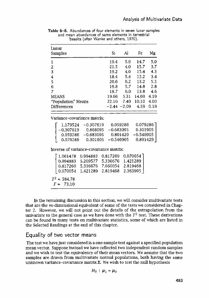
Analysis of Multivariate Data
Table 6-6. Abundances of four elements in seven lunar samples and mean abundances of same elements in terrestrial
basalts (after Wanke and others, 1970).
Lunar Samples Si Al Fe Mg
1 19.4 2 21.5 3 19.2 4 18.4 5 20.6 6 19.8 7 18.7 MEANS 19.66 “Population” Means 22.10 Differences -2.44
5.9 14.7 5.0 4.0 15.7 3.7 4.0 15.4 4.3 5.4 15.2 3.4 6.2 13.2 5.5 5.7 14.8 2.8 6.0 13.8 4.6
5.31 14.69 4.19 7.40 10.10 4.00
-2.09 4.59 0.19
Variance-covariance matrix:
1 1.179524 -0.307619 0.059286 0.079286 -0.307619 0.868095 -0.683095 0.301905
0.059286 -0.683095 0.801429 -0.546905 0.079286 0.301905 -0.546905 0.891429
Inverse of variance-covariance matrix: 1.061478 0.994883 0.817269 0.070054 0.994883 5.209577 5.336676 1.421289 0.817269 5.336676 7.660054 2.819468 0.070054 1.421289 2.819468 2.363995
T 2 = 584.78 F = 73.10
In the remaining discussion in this section, we will consider multivariate tests that are the m-dimensional equivalent of some of the tests we considered in Chap- ter 2. However, we will not point out the details of the extrapolation from the univariate to the general case as we have done with the T 2 test. These derivations can be found in many texts on multivariate statistics, some of which are listed in the Selected Readings at the end of this chapter.
Equality of two vector means The test we have just considered is a one-sample test against a specified population mean vector. Suppose instead we have collected two independent random samples and we wish to test the equivalency of their mean vectors. We assume that the two samples are drawn from multivariate normal populations, both having the same unknown variance-covariance matrix Z. We wish to test the null hypothesis
Ho : PI = P o
483

Statistics and Data Analysis in Geology - Chapter 6
against
The null hypothesis states that the mean vector of the parent population of the first sample is the same as the mean vector of the parent population from which the second sample was drawn.
The test we must use is a multivariate equivalent of Equation (2.48) on p. 73. In that two-sample t-test, we used a pooled estimate of the population variance based on both samples. Accordingly, we must compute a pooled estimate, S , , of the common variance-covariance matrix from our two multivariate samples. This is done by calculating a matrix of sums of squares and products for each sample. We can use the terminology of discriminant functions and denote the matrix of sums of squares and cross products of sample A as SA; similarly, the matrix from sample B is S B . The pooled estimate of the variance-covariance matrix is
H1 : P1 # P o
S, = ( n A + nB - 2)- l ( s A + s B ) (6.32)
We must next find the difference between the two mean vectors, D = EA - X B . Our T 2 test has the form
nAnB D‘S, lD T 2 =
n A + nB (6.33)
The significance of the T 2 test statistic can be determined by the F-transformation:
T 2 n A + nB - m - 1 ( n A + nB - 2 ) m F = (6.34)
which has m and ( n A + nB - m - 1) degrees of freedom (Morrison, 1990).
Eq ua I ity of varia nce-covaria nce matrices An underlying assumption in the two preceding tests is that the samples are drawn from populations having the same variance-covariance matrix. This is the multi- variate equivalent of the assumption of equal populationvariances necessary to per- form t-tests of means. In practice, an assumption of equality may be unwarranted, because samples which exhibit a high mean often will also have a large variance. You will recall from Chapter 4 that such behavior is characteristic of many geologic variables such as mine-assay values and trace-element concentrations. Equality of variance-covariance matrices may be checked by the following “test of generalized variances” which is a multivariate equivalent of the F-test (Morrison, 1990).
Suppose we have k samples of observations, and have measured m variables on each observation. For each sample a variance-covariance matrix, Sk, may be computed. We wish to test the null hypothesis
against the alternative H1 X i #Ej
The null hypothesis states that all k population variance-covariance matrices are the same. The alternative is that at least two of the matrices are different. Each variance-covariance matrix Si is an estimate of a population matrix Xi. If the parent populations of the k samples are identical, the sample estimates may be
484

Analysis of Multivariate Data
combined to form a pooled estimate of the population variance-covariance matrix. The pooled estimate is created by
(6.35)
where ni is the number of observations in the zth group and the summation over ni gives the total number of all observations in all k samples. This equation is algebraically equivalent to Equation (6.32) when k = 2.
From the pooled estimate of the population variance-covariance matrix, a test statistic, M, can be computed:
The test is based on the difference between the logarithm of the determinant of the pooled variance-covariance matrix and the average of the logarithms of the determinants of the sample variance-covariance matrices. If all the sample matrices are the same, this difference will be very small. As the variances and covariances of the samples deviate more and more from one another, the test statistic will increase. Tables of critical values of M are not widely available, so the transformation
can be used to convert M to an approximate x 2 statistic:
x 2 z MC-l (6.38)
The approximate x 2 value has degrees of freedom equal to v = (1 /2 ) (k - 1) . If all the samples contain the same number of observations, n, Equation (6.37) can be simdified to
(6.39)
The x 2 approximation is good if the number of k samples and m variables do not exceed about 5 and each variance-covariance estimate is based on at least 20 observations.
To illustrate the process of hypothesis testing using multivariate statistics, we will work through the following problem. Note that the number of observations is just sufficient for some of the approximations to be strictly valid; we will consider them to be adequate for the purposes of this demonstration.
In a local area in eastern Kansas, all potable water is obtained from wells. Some of these wells draw from the alluvial fill in stream valleys, while others tap a lime- stone aquifer that also is the source of numerous springs in the region. Residents prefer to obtain water from the alluvium, as they feel it is of better quality. How- ever, the water resources of the alluvium are limited, and it would be desirable for some users to obtain their supplies from the limestone aquifer.
In an attempt to demonstrate that the two sources are equivalent in quality, a state agency sampled wells that tapped each source. The water samples were an- alyzed for chemical compounds that affect the quality of water. Some of the data
485

Statistics and Data Analysis in Geology - Chapter 6
Table 6-7. Multivariate statistics for cation composition of water samples collected from wells in an area of eastern Kansas: x1 = silica, x2 = iron, XJ = magnesium, x4 = sodium + potassium, xg = calcium. Data given in file WELLWATR.TXT.
Vector mean of water from wells in limestone XL = [ 9.760 13.955 30.935 25.930 33.2701
Vector mean of water from wells in alluvium XA = [ 12.055 16.080 34.465 29.910 25.055 ]
Variance-covariance matrix of water from wells in limestone, ISL I = 1.8838 - lo8
1 1
5.1615 0.5134 7.3683 -1.4103 -3.4402 0.5134 21.0247 10.6948 -4.0896 -25.3972 7.3683 10.6948 102.8045 -38.5269 -58.1689
-1.4103 -4.0896 -38.5269 98.8654 7.2520 -3.4402 -25.3972 -58.1689 7.2520 290.8706
S L = I I
Variance-covariance matrix of water from wells in alIuvium, IsAI = 2.1777 - lo8 5.6394 0.7333 8.6868 -2.9822 -4.7095 0.7333 23.1733 12.7656 -4.5593 -26.9878
SA = 8.6868 12.7656 103.3982 -42.3949 -58.1232 -2.9822 -4.5593 -42.3949 106.9525 9.2199 -4.7095 -26.9878 -58.1232 9.2199 275.1616
5.4005 0.6233 8.0275 -2.1962 -4.0749 0.6233 22.0990 11.7302 -4.3244 -26.1925
S p = 8.0275 11.7302 103.1013 -40.4609 -58.1461 -2.1962 -4.3244 -40.4609 102.9089 8.2360 I -4.0749 -26.1925 -58.1461 8.2360 283.0661
Pooled variance-covariance matrix, ISPI = 2.0351 lo8
s-1 = P
Inverse of pooled variance-covariance matrix 0.2101 0.0027 -0.0178 -0.0024 -3.0820 - 0.0027 0.0521 -0.0036 4.9006 . 0.0041
-0.0178 -0.0036 0.0148 0.0051 0.0023 -0.0024 4.9006. lom4 0.0051 0.0116 7.2056 . -3.0820 lo-* 0.0041 0.0023 7.2056 - 0.0044
from these analyses are given in the file WELLWATR.TXT. The variance-covariance matrices, inverses, and determinants for the two data sets and for the pooled data are given in Table 6-7. From these we can test the equivalence of the two vector means. We will assume that the samples have been drawn randomly from multi- variate normal populations.
We must first test the assumption that the variance-covariance matrices for the two samples are equivalent using the test statistic M given in Equation (6.36):
M = (20 + 20 - 2)1n2.0351. lo8 - (19ln1.8838. lo8 + 19h2.1777. lo8) = 0.1804
486

Analysis of Multivariate Data
The transformation factor, C-l , must also be calculated to allow use of the x2 approximation:
6 ( 5 + 1 ) ( 2 - 1 ) 2 * 5 2 + 3 * 5 - 1
c- l= 1 -
= 0.8637 The x2 statistic is approximately 0.1804-0.8637 = 0.1558, with degrees of freedom equal to v = 1/2(2 - 1 ) ( 5 ) ( 5 + 1) = 15.
The critical value of x2 for v = 15 with a 5% level of significance is 25.00. The computed statistic is less than this value and does not fall into the critical region, so we may conclude that there is nothing in our samples which suggests that the variance-covariance structures of the parent populations are different. We may pool the two sample variance-covariance matrices and test the equality of the multivariate means using the T 2 test of Equation (6.33):
T 2 = - 2o 2o 1.4847 = 14.847 20 + 20
The value 1.4847 is the product of the matrix multiplications D’Sp’D specified in Equation (6.33). The T 2 statistic may be converted to an F-statistic by Equation (6.34):
Degrees of freedom are v1 = 5 and vz = ( 2 0 + 20 - 5 - 1) = 34. The crit- ical value for F with 5 and 34 degrees of freedom at the 5% (a = 0.05) level of signhcance is 2.49. Our computed test statistic just exceeds this critical value, so we conclude that our samples do, indeed, indicate a difference in the means of the two populations. In other words, there is a statistically significant difference in composition of water from the two aquifers. This simple test will not pinpoint the chemical variables responsible for this difference, but it does substantiate the natives’ contention that they can tell a difference in the water!
Multivariate techniques equivalent to the analysis-of-variance procedures discussed in Chapter 2 are available. In general, these involve a comparison of two m x m matrices that are the multivariate equivalents of the among-group and within-group sums of squares tested in ordinary analysis of variance. The test statistic consists of the largest eigenvalue of the matrix resulting from the compari- son. We will not consider these tests here because their formulation is complicated and their applications to geologic problems have been, so far, minimal. This is not a reflection on their potential utility, however. Interested readers are referred to chapter 5 of Griffith and Amrhein (1997), which presents worked examples of MANOVA’s applied to problems in geography. Koch and Link (1980) include a brief illustration of the application of multivariate analysis of variance to geochemical data. Statistical details are discussed by Morrison (1990).
Cluster Analysis Cluster analysis is the name given to a bewildering assortment of techniques de- signed to perform classification by assigning observations to groups so each group is more or less homogeneous and distinct from other groups. This is the special forte of taxonomists, who attempt to deduce the lineage of living creatures from
487

Statistics and Data Analysis in Geology - Chapter 6
their characteristics and similarities. Taxonomy is highly subjective and depen- dent upon the individual taxonomist’s skills, developed through years of experi- ence. In this respect, the field is analogous in many ways to geology. As in geology, researchers dissatisfied with the subjectivity and capriciousness of traditional methods have sought new techniques of classification which incorporate the mas- sive data-handling capabilities of the computer. These workers, responsible for many of the advances made in numerical classification, call themselves numerical taxonomists.
Numerical taxonomy has been a center of controversy in biology, much like the suspicion that swirled around factor analysis in the 1930’s and 1940’s and provoked acrimonious debates among psychologists. As in that dispute, the techniques of numerical taxonomy were overzealously promoted by some practitioners. In ad- dition, it was claimed that a numerically derived taxonomy better represented the phylogeny of a group of organisms than could any other type of classification. Al- though this has yet to be demonstrated, rapid progress in genotyping suggests that an objective phylogeny may someday be possible. The conceptual underpinnings of taxonomic methods such as cluster analysis are incomplete; the various cluster- ing methods lie outside the body of multivariate statistical theory, and only limited tests of significance are available (Hartigan, 1975; Milligan and Cooper, 1986; Bock, 1996). Although cluster analysis has become an accepted tool for researchers and there are an increasing number of books on the subject, a more complete statis- tical basis for classification has yet to be fashioned. In spite of this, many of the methods of numerical taxonomy are important in geologic research, especially in the classification of fossil invertebrates and the study of paleoenvironments.
The purpose of cluster analysis is to assemble observations into relatively ho- mogeneous groups or “clusters,” the members of which are at once alike and at the same time unlike members of other groups. There is no analytical solution to this problem, which is common to all areas of classification, not just numerical tax- onomy. Although there are alternative classifications of classification procedures (Sneath and Sokal, 1973; Gordon, 1999), most may be grouped into four general types.
1. Partitioning methods operate on the multivariate observations themselves, or on projections of these observations onto planes of lower dimension. Basically, these methods cluster by finding regions in the space defined by the m vari- ables that are poorly populated with observations, and that separate densely populated regions. Mathematical “partitions” are placed in the sparse regions, subdividing the variable space into discrete classes. Although the analysis is done in the m-dimensional space defined by the variables rather than the n-dimensional space defined by the observations, it proceeds iteratively and may be extremely time-consuming (Aldenderfer and Blashfield, 1984; Gordon, 1999).
2. Arbitrary origin methods operate on the similarity between the observations and a set of arbitrary starting points. If n observations are to be classified into k groups, it is necessary to compute an asymmetric n x k matrix of sim- ilarities between the n samples and the k arbitrary points that serve as initial group centroids. The observation closest or most similar to a starting point is combined with it to form a cluster. Observations are iteratively added to the nearest cluster, whose centroid is then recalculated for the expanded cluster.
488

Analysis of Multivariate Data
3. Mutual similarity procedures group together observations that have a common similarity to other observations. First an n x n matrix of similarities between all pairs of observations is calculated. Then the similarity between columns of this matrix is iteratively recomputed. Columns representing members of a single cluster will tend to have intercorrelations near +1, while having much lower correlations with nonmembers.
4. Hierarchical clustering joins the most similar observations, then successively connects the next most similar observations to these. First an n x n matrix of similarities between all pairs of observations is calculated. Those pairs having the highest similarities are then merged, and the matrix is recomputed. This is done by averaging the similarities that the combined observations have with other observations. The process iterates until the similarity matrix is reduced to 2 x 2. The progression of levels of similarity at which observations merge is displayed as a dendrogram. Hierarchical clustering techniques are most widely applied in the Earth sci-
ences, probably because their development has been closely linked with the numer- ical taxonomy of fossil organisms. Because of the widespread use of heirarchical techniques, we will consider them in some detail.
Suppose we have a collection of objects we wish to arrange into a hierarchical classification. In biology, these objects are referred to as “operational taxonomic units” or OW’S (Sneath and Sokal, 1973). We can make a series of measurements on each object which constitutes our data set. If we have n objects and measure m characteristics, the observations form an n x m data matrix, X. Next, some measure of resemblance or similarity must be computed between every pair of objects; that is, between the rows of the data matrix. Several coefficients of resemblance have been used, including a variation of the correlation coefficient fij in which the roles of objects and variables are interchanged. This can be done by transposing X so rows become columns and vice versa, then calculating f i j in the conventional man- ner (Eq. 2.28; p. 43), following the matrix algorithm given in Chapter 3. Although called “correlation,” this measure is not really a correlation coefficient in the con- ventional sense because it involves “means” and “variances” calculated across all the variables measured on two objects, rather than the means and variances of two variables.
Another commonly used measure of similarity between objects is a standard- ized m-space Euclidean distance, dij. The distance coefficient is computed by
(6.40)
where Xik denotes the kth variable measured on object i and xjk is the kth variable measured on object j. In all, m variables are measured on each object, and dij is the distance between object i and object j. As you would expect, a small distance indicates the two objects are similar or “close together,” whereas a large distance indicates dissimilarity. Commonly, each element in the n x m raw data matrix X is standardized by subtracting the column means and dividing by the column standard deviations prior to computing distance measurements. This ensures that each variable is weighted equally. Otherwise, the distance will be influenced most strongly by the variable which has the greatest magnitude. In some instances this may be desirable, but unwanted effects can creep in through injudicious choice of
489

Statistics and Data Analysis in Geology - Chapter 6
measurement units. As an extreme example, we might measure three perpendicular axes on a collection of pebbles. If we measure two of the axes in centimeters and the third in millimeters, the third axis will have proportionally ten times more influence on the distance coefficient than either of the other two variables.
Other measures of similarity that are less commonly used in the Earth sci- ences include a wide variety of association coefficients which are based on binary (presence-absence) variables or a combination of binary and continuous variables. The most popular of these are the simple matching coefficient, Jaccard’s coeffi- cient, and Cower’s coefficient-all ratios of the presence-absence of properties. They differ primarily in the way that mutual absences (called “negative matches”) are considered. Sneath and Sokal (1973) discuss the relative merits of these and other coefficients of association. Probabilistic similarity coefficients are used with binary data and consider the gain or loss of information when objects are combined into clusters. Again, Sneath and Sokal(1973) provide a comprehensive summary.
Computation of a similarity measurement between all possible pairs of objects will result in an n x n symmetrical matrix, C. Any coefficient C i j in the matrix gives the resemblance between objects i and j . The next step is to arrange the objects into a hierarchy so objects with the highest mutual similarity are placed together. Then groups or clusters of objects are associated with other groups which they most closely resemble, and so on until all of the objects have been placed into a complete classification scheme. Many variants of clustering have been developed; a consideration of all of the possible alternative procedures and their relative merits is beyond the scope of this book. Rather, we will discuss one simple clustering technique called the weighted pair-group method with arithmetic averaging, and then point out some useful modifications to this scheme.
Extensive discussions of hierarchical and other classification techniques are contained in books by Jardine and Sibson (1971), Sneath and Sokal (1973), Har- tigan (19751, Aldenderfer and Blashfield (1984), Romesburg (1984), Kaufman and Rousseeuw (1990), Backer (1995), and Gordon (1999). Diskettes containing cluster- ing programs are included in some of the these books or are available separately at modest cost. In addition, most personal computer programs for statistical analysis contain modules for hierarchical clustering.
Table 6-8 contains measurements made on six greywacke thin sections, iden- tified as A, B , . . . , F. The values represent the average of the apparent maximum diameters of ten randomly chosen grains of quartz, rock fragment, and feldspar and the average of the apparent maximum diameters of ten intergranular pores in each thin section. The table also gives a symmetric matrix of similarities, in the form of “correlation” coefficients calculated between the six thin sections.
The first step in clustering by a pair-group method is to find the mutually highest correlations in the matrix to form the centers of clusters. The highest correlation (disregarding the diagonal element) in each column of the matrix in Table 6-8 is shown in boldface type. Specimens A and B form mutually high pairs, because A most closely resembles B , and B most closely resembles A. C and D also form mutually high pairs. E most closely resembles D , but these two do not form a mutually high pair because D resembles C more than it does E. To qualify as a mutually high pair, coefficients C i j and C j i must be the highest coefficients in their respective columns.
We can indicate the resemblance between our mutually high pairs in a diagram such as Figure 6-5 a. Object C is connected to D at a level of? = 0.99, indicating
490

Analysis of Multivariate Data
Table 6-8. Average apparent grain diameters measured on thin sections of six greywackes and matrix of “correlations” between thin sections. Highest
“correlation” in each column is indicated in boldface type.
Average diameters in mm
Rock frag- Specimen Pore Quartz ment Feldspar
A 0.24 1.78 0.69 3.32 B 0.48 2.07 2.41 4.78 C 0.76 4.05 1.2 3.21 D 0.23 2.98 0.85 2.06 E 0.04 3.33 3.39 2.63 F 1.98 0.98 2.01 2.02
“Correlations” on initial iteration
A B C D E F A 1 0,9110 0.7671 0.7041 0.4401 -0.1067 B 0.91 10 1 0.5393 0.4996 0.5704 0.1680 C 0.7671 0.5393 1 0.9910 0.5873 -0.7187 D 0.7041 0.4996 0.9910 1 0.6647 -0.7675 E 0.4401 0.5704 0.5873 0.6647 1 -0.3883 F -0.1067 0.168 -0.7187 -0.7675 -0.3883 1
“Correlations” on second iteration
AB CD E F AB 1 0.394 0.505 0.031 CD 0.394 1 0.626 -0.744 E 0.505 0.626 1 -0.388 F 0.031 -0.744 -0.388 1
“Correlations” on third iteration
AB CDE F AB 1 0.450 0.031 CDE 0.450 1 -0.566 F 0.031 -0.566 1
“Correlations” on fourth iteration
ABCDE F ABCDE 1 -0.268 F -0.268 1
the degree of their mutual similarity. In the same manner, A and B are connected at a level of Q = 0.91. This is the first step in the construction of a dendrogrum, or tree diagram, which is the most common way of displaying the results of clustering.
Next, the similarity matrix must be recomputed, treating grouped or clustered elements as a single element. There are several methods for doing this. In the simple technique we are considering, new correlations between all clusters and unclustered objects are recalculated by simple arithmetic averaging. For exam- ple, the new correlation between cluster CD and object E is equal to the sum of the correlations of the elements collZmon to both CD and E, divided by 2 (that is, Q = (0.5873 + 0.6647)/2 = 0.626). Table 6-8 contains the results of these
491

Statistics and Data Analysis in Geology - Chapter 6
-0.5
-1 .o
1 .o
-0.5
-1 .o
-0.5
-1 .o
A B C D E F U
a
A B C D E F T I U
b
A B C D E F
C
Figure 6-5. (a) Dendrogram with initial clusters, CD and AB. (b) Connection of object E t o initial cluster CD. (c) Final connection of two clusters AB and CDE, and connection of isolated object F to CDE, completing dendrogram.
recalculations. Again, the highest correlations in each column are shown in bold- face type.
The clustering procedure is now repeated; mutually high pairs are sought out and clustered. In this cycle, object E joins cluster CD (Fig. 6-5 b) to form cluster CDE. The correlations between cluster CDE and other clusters or individual objects such as F are again found by adding together the common elements and dividing by 2. This process is repeated again and again until all objects and clusters are joined together. The final matrix of similarities will be a 2 x 2 matrix between the last remaining object and everything else collected into a single cluster, as shown in Table 6-8. This indicates that cluster ABCDE has a resemblance o f? = -0.27 with object F. Our dendrogram can then be completed (Fig. 6-5 c).
Clustering is an efficient way of displaying complex relationships among many objects. However, the process of averaging together members of a cluster and treating them as a single new object introduces distortions into the dendrogram. This distortion becomes increasingly apparent as successive levels of clusters are averaged together. We can evaluate the severity of this distortion by examining what numerical taxonomists call the matrix of cophenetic values. This is nothing more than a matrix of apparent correlations contained within the dendrogram. For example, the dendrogram in Figure 6-5 implies that the correlations between C, D , and E , on one hand, with A and B, on the other, are all ? = 0.45. Similarly, the corre- lation between F and E is the same as the correlation between F and D , or between F and any of the other objects. Only the correlations between A and B and between
492
Next Page

APPENDIX
Table A. l . Cumulative probabilities for the standardized normal distribution. Z-scores
the normal distribution. Especially useful critical values shown in bold italics. are standard deviations from the mean. Probabilities are cumulative areas under
Z P Z P Z P Z P -3.00 0.0013 -2.95 0.0016 -2.90 0.0019 -2.85 0.0022 -2.80 0.0026 -2.75 0.0030 -2.70 0.0035 -2.65 0.0040 -2.60 0.0047 -2.57 0.0050 -2.55 0.0054 -2.50 0.0062 -2.45 0.0071 -2.40 0.0082 -2.35 0.0094 -2.33 0.0100 -2.30 0.0107 -2.25 0.0122 -2.20 0.0139 -2.15 0.0158 -2.10 0.0179 -2.05 0.0202 -2.00 0.0228 -1.96 0.0250 -1.95 0.0256 -1.90 0.0287 -1.85 0.0322 -1.80 0.0359 -1.75 0.0401 -1.70 0.0446 -1.65 0.0495 -1.64 0.0500 -1.60 0.0548
-1.55 0.0606 -1.50 0.0668 -1.45 0.0735 -1.40 0.0808 -1.35 0.0885 -1.30 0.0968 -1.28 0.1000 -1.25 0.1056 -1.20 0.1151 -1.15 0.1251 -1.10 0.1357 -1.05 0.1469 -1.00 0.1587 -0.95 0.1711 -0.90 0.1841 -0.85 0.1977 -0.80 0.2119 -0.75 0.2266 -0.70 0.2420 -0.65 0.2578 -0.60 0.2743 -0.55 0.2912 -0.50 0.3085 -0.45 0.3264 -0.40 0.3446 -0.35 0.3632 -0.30 0.3821 -0.25 0.4013 -0.20 0.4207 -0.15 0.4404 -0.10 0.4602 -0.05 0.4801
0.00 0.5000
0.05 0.5199 0.10 0.5398 0.15 0.5596 0.20 0.5793 0.25 0.5987 0.30 0.6179 0.35 0.6368 0.40 0.6554 0.45 0.6736 0.50 0.6915 0.55 0.7088 0.60 0.7257 0.65 0.7422 0.70 0.7580 0.75 0.7734 0.80 0.7881 0.85 0.8023 0.90 0.8159 0.95 0.8289 1.00 0.8413 1.05 0.8531 1.10 0.8643 1.15 0.8749 1.20 0.8849 1.25 0.8944 1.28 0.9000 1.30 0.9032 1.35 0.9115 1.40 0.9192 1.45 0.9265 1.50 0.9332 1.55 0.9394 1.60 0.9452
1.64 0.9500 1.65 0.9505 1.70 0.9554 1.75 0.9599 1.80 0.9641 1.85 0.9678 1.90 0.9713 1.95 0.9744 1.96 0.9750 2.00 0.9772 2.05 0.9798 2.10 0.9821 2.15 0.9842 2.20 0.9861 2.25 0.9878 2.30 0.9893 2.33 0.9900 2.35 0.9906 2.40 0.9918 2.45 0.9929 2.50 0.9938 2.55 0.9946 2.57 0.9950 2.60 0.9953 2.65 0.9960 2.70 0.9965 2.75 0.9970 2.80 0.9974 2.85 0.9978 2.90 0.9981 2.95 0.9984 3.00 0.9987

Statistics and Data Analysis in Geology
Table A.2. Critical values of t for v degrees of freedom and selected levels of significance. For crit ical values in the left-hand tail, change the sign
o f the table value. Crit ical values are given for the right-hand tail.
Significance Level, a, for: One-tailed Test
.001 .005 .01 .025 .05 .1 .2 No. of Degrees Two-tailed Test of Freedom, v .002 .010 .02 .05 .1 .2 .4
1 2 3 4 5 6 7 8 9
10 11 12 13 14 15 16 17 18 19 20 2 1 22 23 24 25 26
3 18.3088 22.3271 10.2 145 7.1732 5.8934 5.2076 4.7853 4.5008 4.2968 4.1437 4.0247 3.9296 3.8520 3.7874 3.7328 3.6862 3.6458 3.6105 3.5794 3.5518 3.5272 3.5050 3.4850 3.4668 3.4502 3.4350
63.6567 9.9248 5.8409 4.6041 4.0322 3.7074 3.4995 3.3554 3.2498 3.1693 3.1058 3.0545 3.0123 2.9768 2.9467 2.9208 2.8982 2.8784 2.8609 2.8453 2.8314 2.8188 2.8073 2.7969 2.7874 2.7787
31.8205 6.9646 4.5407 3.7470 3.3649 3.1427 2.9980 2.8965 2.8214 2.7638 2.7181 2.6810 2.6503 2.6245 2.6025 2.5835 2.5669 2.5524 2.5395 2.5280 2.5176 2.5083 2.4999 2.4922 2.4851 2.4786
12.7062 4.3027 3.1824 2.7764 2.5706 2.4469 2.3646 2.3060 2.2622 2.2281 2.2010 2.1788 2.1604 2.1448 2.1314 2.1 199 2.1098 2.1009 2.0930 2.0860 2.0796 2.0739 2.0687 2.0639 2.0595 2.0555
6.3138 2.9200 2.3534 2.1318 2.0150 1.9432 1.8946 1.8595 1.8331 1.8125 1.7959 1.7823 1.7709 1.7613 1.7531 1.7459 1.7396 1.7341 1.7291 1.7247 1.7207 1.7171 1.7139 1.7109 1.7081 1.7056
3.0777 1.8856 1.6377 1.5332 1.4759 1.4398 1.4149 1.3968 1.3830 1.3722 1.3634 1.3562 1.3502 1.3450 1.3406 1.3368 1.3334 1.3304 1.3277 1.3253 1.3232 1.3212 1.3195 1.3178 1.3163 1.3150
1.3764 1.0607 0.9785 0.9410 0,9195 0.9057 0.8960 0.8889 0.8834 0.8791 0.8755 0.8726 0.8702 0.8681 0.8662 0.8647 0.8633 0.8620 0.8610 0.8600 0.8591 0.8583 0.8575 0.8569 0.8562 0.8557
(Continued)
602

Appendix
Table A.2. Concluded.
Sigdicance Level, a, for: One-tailed Test
No. of Degrees Two-tailed Test .001 .005 .01 .025 .05 .1 .2
of Freedom, v ,002 ,010 .02 .05 .1 .2 .4
27 28 29 30
40 50 60 70 80 90
100 110 120 130 140 150 03
3.4210 3.4082 3.3962 3.3852
3.3069 3.2614 3.2317 3.2108 3.1953 3.1833 3.1737 3.1660 3.1595 3.1541 3.1495 3.1455 3.0902
2.7707 2.7633 2.7564 2.7500
2.7045 2.6778 2.6603 2.6479 2.6387 2.6316 2.6259 2.6213 2.6174 2.6142 2.61 14 2.6090 2.5758
2.4727 2.4671 2.4620 2.4573
2.4233 2.4033 2.3901 2.3808 2.3739 2.3685 2.3642 2.3607 2.3578 2.3554 2.3533 2.3515 2.2364
2.0518 2.0484 2.0452 2.0423
2.02 11 2.0086 2.0003 1.9944 1.9901 1.9867 1.9840 1.9818 1.9799 1.9784 1.9771 1.9759 1.9600
1.7033 1.7011 1.6991 1.6973
1.6839 1.6759 1.6706 1.6669 1.664 1 1.6620 1.6602 1.6588 1.6577 1.6567 1.6558 1.6551 1.6449
1.3137 1.3125 1.3114 1.3104
1.3031 1.2987 1.2958 1.2938 1.2922 1.2910 1.2901 1.2893 1.2886 1.2881 1.2876 1.2872 1.2816
0.8551 0.8546 0.8542 0.8538
0.8507 0.8489 0.8477 0.8468 0.8461 0.8456 0.8452 0.8449 0.8446 0.8444 0.8442 0.8440 0.8416
Table A.3a. Critical values of F for v1 and vz degrees of freedom and 5% (a = 0.05) level o f significance.
d f 1 2 3 4 5 6 7 8 9 1 0 1 5 2 0 2 5 0 0
1 161.45 199.50 215.71 224.58 230.16 233.99 236.77 238.88 240.54 241.88 245.95 248.01 249.26 250.10
2 18.51 19 19.16 19.25 19.30 19.33 19.35 19.37 19.38 19.40 19.43 19.45 19.46 19.46
3 10.13 9.55 9.28 9.12 9.01 8.94 8.89 8.85 8.81 8.79 8.70 8.66 8.63 8.62
4 7.71 6.94 6.59 6.39 6.26 6.16 6.09 6.04 6.00 5.96 5.86 5.80 5.77 5.75
5 6.61 5.79 5.41 5.19 5.05 4.95 4.88 4.82 4.77 4.74 4.62 4.56 4.52 4.50
6 5.99 5.14 4.76 4.53 4.39 4.28 4.21 4.15 4.10 4.06 3.94 3.87 3.83 3.81
(Continued)
603

Statistics and Data Analysis in Geology
Table A.3a. Concluded.
df 1 2 3 4 5 6 7 8 9 1 0 1 5 2 0 2 5 0 3
7
8
9
10
11
12
13
14
15
16
17
18
19
20
21
22
23
24
25
26
27
28
29
30
40
50
60
70
80
90
100
110
120 03
5.59 4.74 4.35 4.12 3.97 3.87 3.79 3.73 3.68 3.64 3.51 3.44 3.4 3.38
5.32 4.46 4.07 3.84 3.69 3.58 3.50 3.44 3.39 3.35 3.22 3.15 3.11 3.08
5.12 4.26 3.86 3.63 3.48 3.37 3.29 3.23 3.18 3.14 3.01 2.94 2.89 2.86
4.96 4.10 3.71 3.48 3.33 3.22 3.14 3.07 3.02 2.98 2.85 2.77 2.73 2.70
4.84 3.98 3.59 3.36 3.20 3.09 3.01 2.95 2.90 2.85 2.72 2.65 2.60 2.57
4.75 3.89 3.49 3.26 3.11 3.00 2.91 2.85 2.80 2.75 2.62 2.54 2.50 2.47
4.67 3.81 3.41 3.18 3.03 2.92 2.83 2.77 2.71 2.67 2.53 2.46 2.41 2.38
4.60 3.74 3.34 3.11 2.96 2.85 2.76 2.70 2.65 2.60 2.46 2.39 2.34 2.31
4.54 3.68 3.29 3.06 2.90 2.79 2.71 2.64 2.59 2.54 2.40 2.33 2.28 2.25
4.49 3.63 3.24 3.01 2.85 2.74 2.66 2.59 2.54 2.49 2.35 2.28 2.23 2.19
4.45 3.59 3.20 2.96 2.81 2.70 2.61 2.55 2.49 2.45 2.31 2.23 2.18 2.15
4.41 3.55 3.16 2.93 2.77 2.66 2.58 2.51 2.46 2.41 2.27 2.19 2.14 2.11
4.38 3.52 3.13 2.90 2.74 2.63 2.54 2.48 2.42 2.38 2.23 2.16 2.11 2.07
4.35 3.49 3.10 2.87 2.71 2.60 2.51 2.45 2.39 2.35 2.20 2.12 2.07 2.04
4.32 3.47 3.07 2.84 2.68 2.57 2.49 2.42 2.37 2.32 2.18 2.10 2.05 2.01
4.30 3.44 3.05 2.82 2.66 2.55 2.46 2.40 2.34 2.30 2.15 2.07 2.02 1.98
4.28 3.42 3.03 2.80 2.64 2.53 2.44 2.37 2.32 2.27 2.13 2.05 2.00 1.96
4.26 3.40 3.01 2.78 2.62 2.51 2.42 2.36 2.30 2.25 2.11 2.03 1.97 1.94
4.24 3.39 2.99 2.76 2.60 2.49 2.40 2.34 2.28 2.24 2.09 2.01 1.96 1.92
4.23 3.37 2.98 2.74 2.59 2.47 2.39 2.32 2.27 2.22 2.07 1.99 1.94 1.90
4.21 3.35 2.96 2.73 2.57 2.46 2.37 2.31 2.25 2.20 2.06 1.97 1.92 1.88
4.20 3.34 2.95 2.71 2.56 2.45 2.36 2.29 2.24 2.19 2.04 1.96 1.91 1.87
4.18 3.33 2.93 2.70 2.55 2.43 2.35 2.28 2.22 2.18 2.03 1.94 1.89 1.85
4.17 3.32 2.92 2.69 2.53 2.42 2.33 2.27 2.21 2.16 2.01 1.93 1.88 1.84
4.08 3.23 2.84 2.61 2.45 2.34 2.25 2.18 2.12 2.08 1.92 1.84 1.78 1.74
4.03 3.18 2.79 2.56 2.40 2.29 2.20 2.13 2.07 2.03 1.87 1.78 1.73 1.69
4.00 3.15 2.76 2.53 2.37 2.25 2.17 2.10 2.04 1.99 1.84 1.75 1.69 1.65
3.98 3.13 2.74 2.50 2.35 2.23 2.14 2.07 2.02 1.97 1.81 1.72 1.66 1.62
3.96 3.11 2.72 2.49 2.33 2.21 2.13 2.06 2.00 1.95 1.79 1.70 1.64 1.60
3.95 3.10 2.71 2.47 2.32 2.20 2.11 2.04 1.99 1.94 1.78 1.69 1.63 1.59
3.94 3.09 2.70 2.46 2.31 2.19 2.10 2.03 1.97 1.93 1.77 1.68 1.62 1.57
3.93 3.08 2.69 2.45 2.30 2.18 2.09 2.02 1.97 1.92 1.76 1.67 1.61 1.56
3.92 3.07 2.68 2.45 2.29 2.18 2.09 2.02 1.96 1.91 1.75 1.66 1.60 1.55
3.85 3.00 2.61 2.38 2.22 2.11 2.02 1.95 1.89 1.84 1.68 1.58 1.52 1.47
604

Appendix
Table A.3b. Critical values of F for v1 and vz degrees of freedom and 2.5% (& = 0.025) level of significance.
d f 1 2 3 4 5 6 7 8 9 1 0 1 5 2 0 2 5 0 0
1
2
3
4
5
6
7
8
9
10
11
12
13
14
15
16
17
18
19
20
2 1
22
23
24
25
26
27
28
29
30
40
50
60
70
80
90
100
110
120 00
647.79
38.51
17.44
12.22
10.01
8.81
8.07
7.57
7.21
6.94
6.72
6.55
6.41
6.30
6.20
6.12
6.04
5.98
5.92
5.87
5.83
5.79
5.75
5.72
5.69
5.66
5.63
5.61
5.59
5.57
799.50 864.16 899.58 921.85 937.11 948.22 956.66 963.28 968.63 984.87 993.10 998.08 1001.41
39.00 39.17 39.25 39.30 39.33 39.36 39.37 39.39 39.40 39.43 39.45 39.46 39.46
16.04 15.44 15.10 14.88 14.73 14.62 14.54 14.47 14.42 14.25 14.17 14.12 14.08
10.65 9.98 9.60 9.36 9.20 9.07 8.98 8.90 8.84 8.66 8.56 8.50 8.46
8.43 7.76 7.39 7.15 6.98 6.85 6.76 6.68 6.62 6.43 6.33 6.27 6.23
7.26 6.60 6.23 5.99 5.82 5.70 5.60 5.52 5.46 5.27 5.17 5.11 5.07
6.54 5.89 5.52 5.29 5.12 4.99 4.90 4.82 4.76 4.57 4.47 4.40 4.36
6.06 5.42 5.05 4.82 4.65 4.53 4.43 4.36 4.30 4.10 4.00 3.94 3.89
5.71 5.08 4.72 4.48 4.32 4.20 4.10 4.03 3.96 3.77 3.67 3.60 3.56
5.46 4.83 4.47 4.24 4.07 3.95 3.85 3.78 3.72 3.52 3.42 3.35 3.31
5.26 4.63 4.28 4.04 3.88 3.76 3.66 3.59 3.53 3.33 3.23 3.16 3.12
5.10 4.47 4.12 3.89 3.73 3.61 3.51 3.44 3.37 3.18 3.07 3.01 2.96
4.97 4.35 4.00 3.77 3.60 3.48 3.39 3.31 3.25 3.05 2.95 2.88 2.84
4.86 4.24 3.89 3.66 3.50 3.38 3.29 3.21 3.15 2.95 2.84 2.78 2.73
4.77 4.15 3.80 3.58 3.41 3.29 3.20 3.12 3.06 2.86 2.76 2.69 2.64
4.69 4.08 3.73 3.50 3.34 3.22 3.12 3.05 2.99 2.79 2.68 2.61 2.57
4.62 4.01 3.66 3.44 3.28 3.16 3.06 2.98 2.92 2.72 2.62 2.55 2.50
4.56 3.95 3.61 3.38 3.22 3.10 3.01 2.93 2.87 2.67 2.56 2.49 2.44
4.51 3.90 3.56 3.33 3.17 3.05 2.96 2.88 2.82 2.62 2.51 2.44 2.39
4.46 3.86 3.51 3.29 3.13 3.01 2.91 2.84 2.77 2.57 2.46 2.40 2.35
4.42 3.82 3.48 3.25 3.09 2.97 2.87 2.80 2.73 2.53 2.42 2.36 2.31
4.38 3.78 3.44 3.22 3.05 2.93 2.84 2.76 2.70 2.50 2.39 2.32 2.27
4.35 3.75 3.41 3.18 3.02 2.90 2.81 2.73 2.67 2.47 2.36 2.29 2.24
4.32 3.72 3.38 3.15 2.99 2.87 2.78 2.70 2.64 2.44 2.33 2.26 2.21
4.29 3.69 3.35 3.13 2.97 2.85 2.75 2.68 2.61 2.41 2.30 2.23 2.18 4.27 3.67 3.33 3.10 2.94 2.82 2.73 2.65 2.59 2.39 2.28 2.21 2.16
4.24 3.65 3.31 3.08 2.92 2.80 2.71 2.63 2.57 2.36 2.25 2.18 2.13 4.22 3.63 3.29 3.06 2.90 2.78 2.69 2.61 2.55 2.34 2.23 2.16 2.11
4.20 3.61 3.27 3.04 2.88 2.76 2.67 2.59 2.53 2.32 2.21 2.14 2.09
4.18 3.59 3.25 3.03 2.87 2.75 2.65 2.57 2.51 2.31 2.20 2.12 2.07
5.42 4.05 3.46 3.13 2.90 2.74 2.62 2.53 2.45 2.39 2.18 2.07 1.99 1.94
5.34 3.97 3.39 3.05 2.83 2.67 2.55 2.46 2.38 2.32 2.11 1.99 1.92 1.87
5.29 3.93 3.34 3.01 2.79 2.63 2.51 2.41 2.33 2.27 2.06 1.94 1.87 1.82
5.25 3.89 3.31 2.97 2.75 2.59 2.47 2.38 2.30 2.24 2.03 1.91 1.83 1.78
5.22 3.86 3.28 2.95 2.73 2.57 2.45 2.35 2.28 2.21 2.00 1.88 1.81 1.75
5.20 3.84 3.26 2.93 2.71 2.55 2.43 2.34 2.26 2.19 1.98 1.86 1.79 1.73
5.18 3.83 3.25 2.92 2.70 2.54 2.42 2.32 2.24 2.18 1.97 1.85 1.77 1.71
5.16 3.82 3.24 2.90 2.68 2.53 2.40 2.31 2.23 2.17 1.96 1.84 1.76 1.70
5.15 3.80 3.23 2.89 2.67 2.52 2.39 2.30 2.22 2.16 1.94 1.82 1.75 1.69
5.04 3.70 3.13 2.80 2.58 2.42 2.30 2.20 2.13 2.06 1.85 1.72 1.64 1.58
605

Statistics and Data Analysis in Geology
Table A.3c. Critical values of F for v1 and vz degrees o f freedom and 1% ((x = 0.01) level of significance.
df 1 2 3 4 5 6 7 8 9 10 15 20 25 W
1 4052.18 4999.50 5403.35 5624.58 5763.65 5858.99 5928.36 5981.07 6022.47 6055.85 6157.28 6208.73 6239.83 6260.65
2
3
4
5
6 7
8
9
10
11
1 2
13
14
15
16
17
18
19
20
21
22
23
24
25
26
27
28
29
30
40
50
60
70
80
90
100
110
120 W
98.50
34.12
21.20
16.26
13.75
12.25
11.26
10.56
10.04
9.65
9.33
9.07
8.86
8.68
8.53
8.40
8.29
8.18
8.10
8.02
7.95
7.88
7.82
7.77
7.72
7.68
7.64
7.60
7.56
7.3 1
7.17
7.08
7.01
6.96
6.93
6.90
6.87
6.85
6.66
99.00
30.82
18.00
13.27
10.92
9.55
8.65
8.02
7.56
7.21
6.93
6.70
6.51
6.36
6.23
6.11
6.01
5.93
5.85
5.78
5.72
5.66
5.61
5.57
5.53
5.49
5.45
5.42
5.39
5.18
5.06
4.98
4.92
4.88
4.85
4.82
4.80
4.79
4.63
99.17
29.46
16.69
12.06
9.78
8.45
7.59
6.99
6.55
6.22
5.95
5.74
5.56
5.42
5.29
5.18
5.09
5.01
4.94
4.87
4.82
4.76
4.72
4.68
4.64
4.60
4.57
4.54
4.51
4.31
4.20
4.13
4.07
4.04
4.01
3.98
3.96
3.95
3.80
99.25
28.71
15.98
11.39
9.15
7.85
7.01
6.42
5.99
5.67
5.41
5.21
5.04
4.89
4.77
4.67
4.58
4.50
4.43
4.37
4.31
4.26
4.22
4.18
4.14
4.11
4.07
4.04
4.02
3.83
3.72
3.65
3.60
3.56
3.53
3.51
3.49
3.48
3.34
99.30
28.24
15.52
10.97
8.75
7.46
6.63
6.06
5.64
5.32
5.06
4.86
4.69
4.56
4.44
4.34
4.25
4.17
4.10
4.04
3.99
3.94
3.90
3.85
3.82
3.78
3.75
3.73
3.70
3.51
3.41
3.34
3.29
3.26
3.23
3.21
3.19
3.17
3.04
99.33
27.91
15.21
10.67
8.47
7.19
6.37
5.80
5.39
5.07
4.82
4.62
4.46
4.32
4.20
4.10
4.01
3.94
3.87
3.81
3.76
3.71
3.67
3.63
3.59
3.56
3.53
3.50
3.47
3.29
3.19
3.12
3.07
3.04
3.01
2.99
2.97
2.96
2.82
99.36
27.67
14.98
10.46
8.26
6.99
6.18
5.61
5.20
4.89
4.64
4.44
4.28
4.14
4.03
3.93
3.84
3.77
3.70
3.64
3.59
3.54
3.50
3.46
3.42
3.39
3.36
3.33
3.30
3.12
3.02
2.95
2.91
2.87
2.84
2.82
2.81
2.79
2.66
99.37
27.49
14.80
10.29
8.10
6.84
6.03
5.47
5.06
4.74
4.50
4.30
4.14
4.00
3.89
3.79
3.71
3.63
3.56
3.51
3.45
3.41
3.36
3.32
3.29
3.26
3.23
3.20
3.17
2.99
2.89
2.82
2.78
2.74
2.72
2.69
2.68
2.66
2.53
99.39
27.35
14.66
10.16
7.98
6.72
5.91
5.35
4.94
4.63
4.39
4.19
4.03
3.89
3.78
3.68
3.60
3.52
3.46
3.40
3.35
3.30
3.26
3.22
3.18
3.15
3.12
3.09
3.07
2.89
2.78
2.72
2.67
2.64
2.61
2.59
2.57
2.56
2.43
99.40
27.23
14.55
10.05
7.87
6.62
5.81
5.26
4.85
4.54
4.30
4.10
3.94
3.80
3.69
3.59
3.51
3.43
3.37
3.31
3.26
3.21
3.17
3.13
3.09
3.06
3.03
3.00
2.98
2.80
2.70
2.63
2.59
2.55
2.52
2.50
2.49
2.47
2.34
99.43
26.87
14.20
9.72
7.56
6.31
5.52
4.96
4.56
4.25
4.01
3.82
3.66
3.52
3.41
3.31
3.23
3.15
3.09
3.03
2.98
2.93
2.89
2.85
2.81
2.78
2.75
2.73
2.70
2.70
2.52
2.42
2.35
2.31
2.27
2.24
2.22
2.21
2.06
99.45
26.69
14.02
9.55
7.40
6.16
5.36
4.81
4.41
4.10
3.86
3.66
3.51
3.37
3.26
3.16
3.08
3.00
2.94
2.88
2.83
2.78
2.74
2.70
2.66
2.63
2.60
2.57
2.55
2.55
2.37
2.27
2.20
2.15
2.12
2.09
2.07
2.05
1.90
99.46
26.58
13.91
9.45
7.30
6.06
5.26
4.71
4.31
4.01
3.76
3.57
3.41
3.28
3.16
3.07
2.98
2.91
2.84
2.79
2.73
2.69
2.64
2.60
2.57
2.54
2.51
2.48
2.45
2.45
2.27
2.17
2.10
2.05
2.01
1.99
1.97
1.95
1.79
99.47
26.50
13.84
9.38
7.23
5.99
5.20
4.65
4.25
3.94
3.70
3.51
3.35
3.21
3.10
3.00
2.92
2.84
2.78
2.72
2.67
2.62
2.58
2.54
2.50
2.47
2.44
2.41
2.39
2.39
2.20
2.10
2.03
1.98
1.94
1.92
1.89
1.88
1.72
606

Appendix
Table A.4. Critical values of x2 for v degrees o f freedom and selected levels of significance.
No. of Degrees of Freedom, v 0.20 0.10 0.05 0.025 0.01
Significance Level, a
1 2 3 4 5 6 7 8 9
10 11 12 13 14 1 5 16 17 18 19 20 21 22 23 24 25 26 27 28 29 30
40 50 60
1.64 3.22 4.64 5.99 7.29 8.56 9.80
11.03 12.24 13.44 14.63 15.81 16.98 18.15 19.31 20.47 21.61 22.76 23.90 25.04 26.17 27.30 28.43 29.55 30.68 31.79 32.91 34.03 35.14 36.25
47.27 58.16 68.97
2.71 4.61 6.2 5 7.78 9.24
10.64 12.02 13.36 14.68 15.99 17.28 18.55 19.81 21.06 22.31 23.54 24.77 25.99 27.20 28.41 29.62 30.81 32.01 33.20 34.38 35.56 36.74 37.92 39.09 40.26
51.81 63.17 74.40
(Con t in ued)
3.84 5.99 7.81 9.49
11.07 12.59 14.07 15.51 16.92 18.31 19.68 2 1.03 22.36 23.68 25.00 26.30 27.59 28.87 30.14 31.41 32.67 33.92 35.17 36.42 37.65 38.89 40.11 41.34 42.56 43.77
55.76 67.50 79.08
5.02 7.38 9.35
11.14 12.83 14.45 16.01 17.53 19.02 20.48 21.92 23.34 24.74 26.12 2 7.49 28.85 30.19 31.53 32.85 34.17 35.48 36.78 38.08 39.36 40.65 41.92 43.19 44.46 45.72 46.98
59.34 71.42 83.30
6.63 9.21
11.34 13.28 15.09 16.81 18.48 20.09 21.67 23.21 24.72 26.22 27.69 29.14 30.58 32.00 33.41 34.81 36.19 37.57 38.93 40.29 41.64 42.98 44.31 45.64 46.96 48.28 49.59 50.89
63.69 76.15 88.38
607

Statistics and Data Analysis in Geology
Table A.4. Concluded.
No. of Degrees of Freedom, v 0.20 0.10 0.05 0.02 5 0.01
Significance Level, cx
70 79.71 85.53 90.5 3 95.02 100.43 80 90.41 96.58 101.88 106.63 112.33 90 101.05 107.57 113.15 118.14 124.12
100 111.67 118.50 124.34 129.56 135.81 110 122.25 129.39 135.48 140.92 147.41 120 132.81 140.23 146.57 152.21 158.95
Table A.5. Probabilities of occurrence o f specified values of the Mann-Whitney W, statistic for testing the equality t o two samples of size n and m, where
m 5 n I 8. CL is the lower critical value and Cu is the upper critical value.'
m = 3
CL 3 cu 4 cu 5 Cu 6 Cu 7 Cu 8 Cu n
6 .0500 15 7 .lo00 14 8 .2000 13 9 .3500 12
10 .5000 1 1 1 1 .6500 10 12 .8000 9 13 .9000 8 14 .9500 7 15 1.0000 6 16 17 18 19 20 21 22 23 24
.0286
.0571 ,1143 .zoo0 .3143 .4286 .5714 .6857 ,8000 .8857
.942 .9714
1.0000
18 .0179 17 .0357 16 .0714 15 .1250 14 .1964 13 .2857 12 .3929 1 1 .5000 10 .6071 9 .7143 8 .8036 7 .8750 6 .9286
.9643
.982 1 1.0000
21 20 19 18 17 16 15 14 13 12 1 1 10 9 8 7 6
.0119
.0238
.0476 ,0833 .1310 .1905 .2738 .3571 .4524 S476 .6429 .7262 .8095 .8690 .9167 .9524 .9762 .9881
1.0000
24 23 22 21 20 19 18 17 16 15 14 13 12 1 1 10 9 8 7 6
.0083
.0167
.0333
.0583
.0917
.1333
.1917
.2583 ,3333 .4167 .5000 .5833 .6667 .7417 .8083 .8667 .9083 .94 17 .9667
27 26 25 24 23 22 21 20 19 18 17 16 15 14 13 12 1 1 10 9
.0061
.0121
.0242
.0424
.0667
.0970
.1394
.1879
.2485 ,3152 .3879 .4606 .5394 .6121 .6848 .7515 .8121 .8606 .9030
30 29 28 27 26 25 24 23 22 21 20 19 18 17 16 15 14 13 12
'Adapted from S. Siege1 and N.J. Castellan, Jr., 1988, Nonparametric Statistics for the Behavioral Sciences, Zed. Reproduced by permission of The McGraw-Hill Companies, New York.
(Con t in ued)
608

Appendix
Table A.5. Continued.
m = 4 n CL 4 cu 5 Cu 6 Cu 7 Cu 8 Cu
10 .0143 26 .0079 30 .0048 34 .0030 38 .0020 42 1 1 .0286 25 .0159 29 .0095 33 .0061 37 .0040 41 12 ,0571 24 ,0317 28 .0190 32 .0121 36 .0081 40 13 .lo00 23 ,0556 27 .0333 31 .0212 35 .0141 39 14 .1714 22 .0952 26 ,0571 30 .0364 34 .0242 38 15 ,2429 21 .1429 25 .0857 29 .0545 33 .0364 37 16 ,3429 20 .2063 24 .1286 28 .0818 32 .0545 36 17 ,4429 19 .2778 23 .1762 27 .1152 31 .0768 35 18 .5571 18 ,3651 22 .2381 26 .1576 30 .lo71 34 19 .6571 17 ,4524 21 .3048 25 .2061 29 .1414 33 20 ,7571 16 .5476 20 .3810 24 .2636 28 .1838 32 21 .8286 15 .6349 19 .4571 23 .3242 27 .2303 31 22 ,9000 14 .7222 18 .5429 22 .3939 26 .2848 30 23 .9429 13 .7937 17 .6190 21 .4636 25 .3414 29 24 .9714 12 .8571 16 .6952 20 .5364 24 .4040 28 25 ,9857 1 1 .9048 15 .7619 19 .6061 23 .4667 27 26 1.0000 10 ,9444 14 .8238 18 .6758 22 .5333 26 27 ,9683 13 .8714 17 .7364 21 .5960 25 28 .9841 12 .9143 16 .7939 20 .6586 24 29 ,9921 1 1 .9429 15 .8424 19 .7152 23 30 1.0000 10 .9667 14 .8848 18 .7697 22 31 ,9810 13 .9182 17 .8162 21 32 .9905 12 .9455 16 .8586 20 33 .9952 1 1 .9636 15 .8929 19 34 1.0000 10 .9788 14 .9232 18
(Continued)
609

Statistics and Data Analysis in Geology
Table A.5. Continued.
15 16 17 18 19 20 21 22 23 24 25 26 27 28 29 30 31 32 33 34 35 36 37 38 39 40
,0040 40 ,0079 39 .0159 38 .0278 37 ,0476 36 .0754 35 ,1111 34 .1548 33 .2103 32 .2738 31 .3452 30 .4206 29 .5000 28 .5794 27 .6548 26 .7262 25 ,7897 24 .8452 23 ,8889 22 .9246 21 ,9524 20 .9722 19 .9841 18 .9921 17 .9960 16
1.0000 15
.0043 44
.0087 43
.0152 42
.0260 41
.0411 40
.0628 39
.0887 38
.1234 37
.1645 36
.2143 35
.2684 34
.3312 33
.3961 32
.4654 31
.5346 30
.6039 29
.6688 28
.7316 27
.7857 26
.8355 25
.8766 24
.9113 23
.9372 22
.9589 21 ,9740 20
n m = 5
CL 5 c u 6 cu 7 cu 8 cu .0013 50 .0008 55 .0022 45 .0025 49 .0051 48 .0088 47 .0152 46 .0240 45 ,0366 44 ,0530 43 .0745 42 ,1010 41 .1338 40 ,1717 39 ,2159 38 ,2652 37 ,3194 36 ,3775 35 .4381 34 ,5000 33 .5619 32 ,6225 31 .6806 30 .7348 29 .7841 28 .8283 27 .8662 26 .8990 25
.0016 54
.0031 53
.0054 52
.0093 51
.0148 50
.0225 49
.0326 48
.0466 47
.0637 46
.0855 45
.1111 44
.1422 43
.1772 42
.2176 41
.2618 40
.3108 39
.3621 38
.4165 37
.4716 36
.5284 35
.5835 34
.6379 33
.6892 32
.7382 31
.7824 30
(Continued)
610

Appendix
Table A.5. Continued.
m = 6 n CL 6 cu 7 cu 8 cu 21 22 23 24 25 26 27 28 29 30 31 32 33 34 35 36 37 38 39 40 41 42 43 44 45 46 47 48 49 50 51
.0011 57
.0022 56
.0043 55
.0076 54 ,0130 53 .0206 52 .0325 51 .0465 50 .0660 49 .0898 48 .1201 47 ,1548 46 .1970 45 ,2424 44 .2944 43 .3496 42 ,4091 41 .4686 40 ,5314 39 .5909 38 .6504 37 .7056 36 .7576 35 .8030 34 A452 33 A799 32 .9102 31 .9340 30 .9535 29 .9675 28 .9794 27
.0006 63 ,0012 62 ,0023 61 ,0041 60 .0070 59 .0111 58 .0175 57 .0256 56 .0367 55 .0507 54 .0688 53 .0903 52 ,1171 51 .1474 50 .1830 49 ,2226 48 .2669 47 .3141 46 .3654 45 ,4178 44 .4726 43 .5274 42 .5822 41 .6346 40 .6859 39 .7331 38 .7774 37 A170 36 A526 35 .8829 34 .9097 33
.0003 69
.0007 68
.0013 67
.0023 66
.0040 65
.0063 64
.0100 63
.0147 62 ,0213 61 .0296 60 .0406 59 .0539 58 .0709 57 .0906 56 .1142 55 .1412 54 .1725 53 .2068 52 .2454 51 .2864 50 .3310 49 .3773 48 .4259 47 .4749 46 .5251 45 .5741 44 .6227 43 .6690 42 .7136 41 .7546 40 .7932 39
(Continued)
611

Statistics and Data Analysis in Geology
Table A.5. Concluded.
28 29 30 31 32 33 34 35 36 37 38 39 40 41 42 43 44 45 46 47 48 49 50 51 52 53 54 55 56 57 58 59 60 61 62 63
.0003 77
.0006 76
.0012 75
.0020 74
.0035 73
.0055 72
.0087 71
.0131 70
.0189 69
.0265 68
.0364 67
.0487 66
.0641 65
.0825 64
.lo43 63
.1297 62
.1588 61
.1914 60
.2279 59
.2675 58
.3100 57
.3552 56
.4024 55
.4508 54
.5000 53
.5492 52
.5976 51
.6448 50
.6900 49
.7325 48
.7721 47
.8086 46 A412 45 A703 44 A957 43 .9175 42
.0002
.0003
.0006
.0011
.0019
.0030
.0047
.0070
.0103
.0145
.0200
.0270
.0361
.0469
.0603
.0760
.0946
.1159
.1405
.1678
.1984
.2317
.2679
.3063
.3472
.3894
.4333
.4775
.5225
.5667
.6106
.6528
.6937
.7321
.7683
.8016
84 83 82 81 80 79 78 77 76 75 74 73 72 71 70 69 68 67 66 65 64 63 62 61 60 59 58 57 56 55 54 53 52 51 50 49
36 37 38 39 40 41 42 43 44 45 46 47 48 49 50 51 52 53 54 55 56 57 58 59 60 61 62 63 64 65 66 67 68 69 70 71 72 73 74 75 76
.0001 100 ,0002 99 .0003 98 .0005 97 .0009 96 .0015 95 .0023 94 .0035 93 .0052 92 ,0074 91 ,0103 90 ,0141 89 .0190 88 .0249 87 .0325 86 .0415 85 ,0524 84 .0652 83 ,0803 82 .0974 81 .1172 80 .1393 79 .1641 78 .1911 77 .2209 76 .2527 75 ,2869 74 ,3227 73 ,3605 72 .3992 71 .4392 70 ,4796 69 .5204 68 ,5608 67 .6008 66 .6395 65 .6773 64 .7131 63 .7473 62 .7791 61 .8089 60
612

Appendix
Table A.6. Critical values o f Spearman's p for testing the significance of a rank correlation. Table gives upper critical value of Spearman's p
for specified level of significance. Lower critical values are equal t o - p .
Significance, ct, for One-tailed Test
Significance, a, for Two-tailed Test .10 .05 -02 5 .01 .005 .001
.20 .10 .05 .02 .01 .002
n 4 5 6 7 8 9
10 11 12 13 14 1 5 16 17 18 19 20 21 22 23 24 25 26 27 28 29 30
.8000
.7000
.6000
.5357
.so00
.4667
.4424
.4182
.3986
.3791
.3626
.3500
.3382
.3260
.3148
.3070
.2977
.2909
.2829
.2767
.2704
.2646
.2588
.2540
.2490
.2443
.2400
.8000
.8000 ,7714 .6786 .6190 .5833 .5515 .5273 .4965 .4780 ,4593 .4429 .4265 .4118 .3994 .3895 .3789 .3688 .3597 .3518 .3435 ,3362 .3299 .3236 .3175 .3113 .3059
.goo0
.8286
.7450
.7143
.6833 ,6364 .6091 .5804 . 5 549 .5341 .5179 ,5000 .4853 .4716 .4 5 79 .4451 .4351 .4241 .4150 .4061 .3977 .3894 .3822 .3749 .3685 .3620
.goo0
.8857
.8571
.8095
.7667
.7333
.7000
.6713
.6429
.6220
.6000
.5824
.5637
.5480
.5333
.5203
.5078
.4963
.4852
.4748
.4654
.4 5 64
.4481
.4401
.4320
.4251
.9429
.8929
.8571
.8167
.7818
.7455
.7273
.6978
.6747
.6536
.6324
.6152
.5975
.5825
.5684 ,5545 .5426 .5306 ,5200 .5100 .SO02 .4915 ,4828 .4 744 .4665
.9643
.9286
.g000
.8667
.8364
.8182
.7912
.7670
.7464
.7265
.7083
.6904
.6737
.6586
.6455
.6318
.6186
.6070
.5962
.5856
.5757
.5660
.5567
.5479
613

Statistics and Data Analysis in Geology
Table A.7. Critical values of D in the Kolmogorov-Smirnov goodness-of-fit test.
Significance, a, for One-tailed Test
Significance, a, for Two-tailed Test 0.1 0.05 0.02 5 0.05 0.02 0.01
0.2 0.1 0.05 0.02 5 0.01 0.005 n 1 2 3 4 5 6 7 8 9
10 11 1 2 13 14 1 5 16 17 18 19 20 2 1 22 23 24 25 26 27 28 29 30 31 32 33 34 35 36 37 38 39 40
0.7275 0.5551 0.4671 0.4 114 0.3720 0.3422 0.3187 0.2995 0.2834 0.2697 0.2579 0.2474 0.2382 0.2299 0.2225 0.2157 0.2096 0.2039 0.1986 0.1938 0.1893 0.1851 0.1812 0.1775 0.1740 0.1707 0.1676 0.1647 0.1619 0.1593 0.1568 0.1 544 0.1521 0.1499 0.1478 0.1458 0.1438 0.1420 0.1402 0.1385
0.8721 0.6655 0.5600 0.4932 0.4460 0.4103 0.3821 0.3591 0.3398 0.3234 0.3092 0.2967 0.2856 0.2757 0.2668 0.2586 0.2513 0.2444 0.2382 0.2323 0.2270 0.2219 0.2172 0.2128 0.2086 0.2047 0.2010 0.1975 0.1941 0.1910 0.1880 0.1851 0.1823 0.1797 0.1772 0.1748 0.1725 0.1702 0.1681 0.1660
0.9950 0.7592 0.6389 0.5627 0.5088 0.4681
0.436 0.4097 0.3877 0.3689 0.3527 0.3385 0.3258 0.3145 0.3043 0.2951 0.2866 0.2789 0.2717 0.2651 0.2589 0.2532 0.2478 0.2428 0.2380 0.2335 0.2293 0.2253 0.2215 0.2179 0.2144 0.2112 0.2080 0.2050 0.2021 0.1994 0.1967 0.1942 0.1917 0.1894
0.9999 0.8425 0.7090 0.6244 0.5646 0.5195 0.4838 0.4546 0.4302 0.4094 0.3914 0.3756 0.3616 0.3490 0.3377 0.3274 0.3181 0.3095 0.301 5 0.2942 0.2873 0.2810 0.2750 0.2694 0.2641 0.2591 0.2544 0.2500 0.2458 0.2418 0.2379 0.2343 0.2308 0.2275 0.2243 0.2212 0.2183 0.2155 0.2128 0.2102
0.9999 0.94 13 0.7922 0.6977 0.6309 0.5804 0.5405 0.5080 0.4807 0.4575 0.4373 0.4196 0.4040 0.3900 0.3773 0.3659 0.3554 0.3458 0.3369 0.3287 0.3211 0.3 139 0.3072 0.3010 0.2951 0.2895 0.2843 0.2793 0.2746 0.2701 0.2659 0.2618 0.2579 0.2542 0.2506 0.2472 0.2439 0.2408 0.2377 0.2348
0.9999 0.9999 0.8497 0.7483 0.6767 0.6226 0.5798 0.5448 0.5156 0.4907 0.4691 0.4501 0.4333 0.4183 0.4048 0.3924 0.3812 0.3709 0.3614 0.3526 0.3443 0.3367 0.3296 0.3228 0.3166 0.3106 0.3049 0.2996 0.2946 0.2897 0.2852 0.2808 0.2766 0.2726 0.2688 0.2652 0.2616 0.2582 0.2550 0.2519
(Continued)
614

Appendix
Table A.7. Continued.
Significance, a, for One-tailed Test
Significance, a, for Two-tailed Test 0.1 0.05 0.025 0.05 0.02 0.01
0.2 0.1 0.05 0.02 5 0.01 0.005
41 42 43 44 45 46 47 48 49 50 51 52 53 54 55 56 57 58 59 60 61 62 63 64 65 66 67 68 69 70 71 72 73 74 75 76 77 78 79 80
0.1368 0.1352 0.1337 0.1322 0.1307 0.1293 0.1280 0.1267 0.1254 0.1242 0.1230 0.1218 0.1206 0.1196 0.1185 0.1174 0.1164 0.1155 0.1145 0.1135 0.1126 0.1117 0.1108 0.1100 0.1092 0.1084 0.1075 0.1068 0.1060 0.1053 0.1045 0.1038 0.1031 0.1024 0.1017 0.1011 0.1004 0.0998 0.0992 0.0986
0.1640 0.1621 0.1602 0.1585 0.1567 0.1551 0.1534 0.1519 0.1503 0.1488 0.1474 0.1460 0.1447 0.1433 0.1421 0.1408 0.1396 0.1384 0.1373 0.1361 0.1350 0.1340 0.1329 0.1319 0.1309 0.1299 0.1290 0.1280 0.1271 0.1262 0.1253 0.1245 0.1236 0.1228 0.1220 0.1212 0.1204 0.1197 0.1189 0.1182
0.1871 0.1849 0.1828 0.1808 0.1788 0.1769 0.1751 0.1732 0.1715 0.1698 0.1682 0.1666 0.1650 0.1635 0.1621 0.1606 0.1 592 0.1579 0.1566 0.1553 0.1540 0.1528 0.1516 0.1505 0.1493 0.1482 0.1471 0.1460 0.1450 0.1440 0.1430 0.1420 0.1411 0.1401 0.1392 0.1383 0.1374 0.1365 0.1357 0.1348
(Con t in ued)
0.2076 0.2052 0.2029 0.2006 0.1984 0.1963 0.1942 0.1923 0.1903 0.1885 0.1866 0.1849 0.1831 0.1815 0.1798 0.1783 0.1767 0.1753 0.1738 0.1723 0.1709 0.1696 0.1683 0.1670 0.1657 0.1645 0.1633 0.1621 0.1609 0.1598 0.1587 0.1576 0.1565 0.1555 0.1544 0.1534 0.1525 0.1515 0.1506 0.1496
0.2320 0.2293 0.2267 0.2241 0.2217 0.2193 0.2170 0.2148 0.2126 0.2106 0.2085 0.2065 0.2046 0.2028 0.2010 0.1992 0.1975 0.1958 0.1941 0.1926 0.1910 0.1895 0.1880 0.1866 0.1851 0.1838 0.1824 0.1811 0.1798 0.1785 0.1773 0.1761 0.1749 0.1737 0.1726 0.1714 0.1703 0.1693 0.1682 0.1672
0.2489 0.2460 0.2431 0.2404 0.2378 0.2353 0.2328 0.2304 0.2281 0.2259 0.2237 0.2216 0.2195 0.2175 0.2155 0.2137 0.2118 0.2100 0.2082 0.2065 0.2049 0.2033 0.2017 0.2001 0.1986 0.1971 0.1957 0.1942 0.1928 0.1915 0.1901 0.1888 0.1876 0.1863 0.1851 0.1839 0.1827 0.1816 0.1805 0.1793
615

Statistics and Data Analysis in Geology
Table A.7. Concluded.
Significance, LX, for One-tailed Test
Significance, a, for Two-tailed Test 0.1 0.05 0.02 5 0.05 0.02 0.01
0.2 0.1 0.05 0.02 5 0.01 0.005
81 82 83 84 85 86 87 88 89 90 91 92 93 94 95 96 97 98 99
100
0.0980 0.0974 0.0968 0.0962 0.0957 0.0951 0.0946 0.0941 0.093 5 0.0930 0.092 5 0.0920 0.091 5 0.091 1 0.0906 0.0901 0.0897 0.0892 0.0888 0.0883
0.1175 0.1168 0.1161 0.1154 O.Il47 0.1141 0.1134 0.1128 0.1121 0.1115 0.1109 0.1103 0.1097 0.1092 0.1086 0.1081 0.1075 0.1069 0.1064 0.1059
0.1340 0.1332 0.1324 0.1316 0.1309 0.1301 0.1294 0.1287 0.1279 0.1272 0.1265 0.1259 0.1252 0.1245 0.1239 0.1233 0.1226 0.1220 0.1214 0.1208
0.1487 0.1478 0.1470 0.1461 0.1452 0.1444 0.1436 0.1428 0.1420 0.1412 0.1404 0.1397 0.1390 0.1382 0.1375 0.1368 0.1361 0.1354 0.1347 0.1341
0.1662 0.1652 0.1642 0.1632 0.1623 0.1613 0.1604 0.1595 0.1586 0.1578 0.1569 0.1561 0.1552 0.1544 0.1536 0.1528 0.1520 0.1513 0.1505 0.1498
0.1782 0.1772 0.1761 0.1751 0.1741 0.1730 0.1721 0.1711 0.1702 0.1692 0.1683 0.1674 0.1665 0.1656 0.1648 0.1639 0.1631 0.1623 0.1614 0.1607
616

Appendix
Table A.8. Critical values of the Lilliefors test statistic, T, for testing goodness-of-fit to a normal distribution.
Level of Significance, a .20 .15 .10 .05 .01
Sample size, n = 4
5 6 7 8 9
10 11 1 2 13 14 1 5 16 17 18 19 20 25 30
>30
.300 ,285 .265 .247 .233 .223 .215 .206 .199 ,190 .183 .177 .173 .169 .166 .163 .160 .142 .131
fi .736 -
.319
.299
.277 ,258 ,244 .233 ,224 .217 .212 .202 .194 .187 ,182 .177 .173 .169 ,166 ,147 .136
fi .768 -
.352
.315
.294
.276
.261
.249 ,239 .230 ,223 .214 .207 .201 .195 .189 .184 .179 .174 .158 .144
fi A05
.381 .417
.337 .405
.319 .364
.300 .348
.285 .331
.271 .311
.258 .294
.249 ,284
.242 .275
.234 .268
.227 .261
.220 .257
.213 .250
.206 ,245
.200 .239
.195 .235
.190 .231
.173 .200
.161 .187
fi fi .886 - 1.031 -
617

Statistics and Data Analysis, in Geology
Table A.9. Maximum likelihood estimates of the concentration parameter K for calculated values of a (adapted from Batschelet, 1965;
and Gumbel, Greenwood, and Durand, 1953). - i? K i? K R K
0.00 0.00000 .01 .02000 .02 .04001 .03 .06003 .04 .08006 .05 .lo013 .06 .12022 .07 .14034 .08 .16051 .09 .18073 .10 .20101 .ll .22134 .12 .24175 .13 .26223 .14 .28279 .15 .30344 .16 ,32419 .17 .34503 .18 .36599 .19 .38707 .20 .40828 .21 .42962 .22 .45110 .23 .47273 .24 .49453 2 5 .51649 .26 .53863 .27 .56097 .28 .58350 2 9 .60625 .30 .62922 .31 .65242 .32 .67587 .33 .69958 .34 .72356
0.35 .36 .37 -38 .39 .40 .4 1 .42 .43 .44 .4 5 .46 .4 7 .48 .49 .so .51 .52 .53 .54 .55 .56 .57 .58 .59 .60 -61 .62 .63 -64 .65 .66 .67 .68 .69
0.74783 .77241 .79730 .82253 .84812 .87408 .go043 .92720 .95440 ,98207
1.01022 1.03889 1.068 10 1.09788 1.12828 1.15932 1.19105 1.22350 1.25672 1.29077 1.32570 1.36156 1.39842 1.43635 1.47543 1.51574 1.55738 1.60044 1.64 506 1.69134 1.73945 1.7895 3 1.841 77 1.89637 1.95357
0.70 .71 -72 .73 -74 .75 -76 -77 .78 .79 .80 .81 .82 .83 .84 .85 .86 .87 .88 .89 .90 .91 -92 .93 .94 .95 .96 .97 .98 .99
1.00
2.01363 2.07685 2.14359 2.21425 2.28930 2.36930 2.45490 2.54686 2.64613 2.75382 2.87129 3.00020 3.14262 3.30114 3.47901 3.68041 3.91072 4.17703 4.48876 4.85871
5.3047 5.8522 6.5394 7.4257 8.6104
10.2716 12.766 1 16.9266 25.2522 50.2421
CQ
618

Appendix
Table A.10. Critical values o f for Rayleigh's test for the presence o f a preferred trend. From Mardia (1972).
Level of Significance, a .10 .05 ,025 .01
~~ ~
Sample size, n = 4
5 6 7 8 9
10 11 12 13 14 15 16 17 18 19 20 21 22 23 24 25 30 35 40 45 50
0.768 .677 .618 .572 .535 .504 .4 78 .456 .437 .420 .405 .391 .379 .367 .357 .348 .339 .331 .323 ,316 ,309 .303 .277 .256 .240 .226 .214
0.847 .754 .690 .642 .602 .569 .540 .516 .494 .475 .458 .443 .429 .417 .405 .394 .385 .375 .367 .359 .351 .344 .315 .292 .273 .257 .244
0.905 .816 .753 ,702 ,660 .624 ,594 .567 ,544 .524 .SO5 .489 .474 .460 ,447 .436 .425 ,415 .405 ,397 .389 .381 .348 .323 ,302 .285 .270
0.960 .879 .825 .771 .725 .687 .655 .62 7 .602 .580 .560 .542 .525 .510 .496 .484 .472 .461 .451 .44 1 .432 .423 .387 .359 .336 .318 .301
619

Statistics and Data Analysis in Geology
Table A.11. Critical values of for the test of uniformity of a spherical distribution.
Level of Significance, a .10 .05 .02 .o 1
Sample size, n = 5
6 7 8 9
10 11 12 13 14 15 16 17 18 19 20 2 1 22 23 24 25 30 35 40 45 50
100
0.637 .583 .541 .SO6 .478 .454 .433 .415 .398 .384 .371 .359 .349 .339 .330 .322 .314 .307 .300 .294 .288
.26
.24
.23
.22
.20
.14
0.700 .642 .597 ,560 .529 .SO3 .480 .460 .442 .427 .413 .400 .388 .377 ,367 .358 .350 .342 .334 .328 .321 .29 .27 .26 .24 .23 .16
0.765 .707 .659 .619 .586 .558 .533 .512 .492 .475 .460 ,446 .443 .42 1 .410 .399 .390 .382 .374 ,366 .359
.33
.31
.29
.27
.26
.18
0.805 .747 .698 .658 .624 .594 ,568 .546 .526 .507 .491 .4 76 ,463 ,450 .438 .428 ,418 .408 .400 .392 .384
.36
.33
.3 1
.29
.28
.19
620

This page has been reformatted by Knovel to provide easier navigation.
INDEX
Index Terms Links
A
Aberfan, Wales (UK) 284
ABOC.TXT 401
accuracy 26
added terms (curvilinear regression) 210
additive rule of probability 21
A.E.C. (Atomic Energy Commission) 154
aerial photograph 445 593
Africa 400
aggregated pattern of points 299
agricultural runoff 589
Agua Caliente Formation (Precambrian) 116
AGUACAL.TXT 116
airborne magnetometer survey 590
airborne radiometric measurement 570
Al2O3 590
Alabama (USA) 285 444
Alaska (USA) 204
Alberta Basin (Canada) 371 403
aliasing 274 365
Allen’s Creek, Indiana (USA) 284
alluvial fill 485
alluvial pediment 446
alternative hypothesis 61
ammonoid 502 505
amphibolite 288
amplitude 267 362
analcime 592
“analysis of associations” 552

Index Terms Links
This page has been reformatted by Knovel to provide easier navigation.
analysis of variance (ANOVA) 78 182 196 204 210 223 288
366 407 464 468 487 572
- clustering 497
- multiple regression 464 468
- nested 88 367 448
- one-way 78 117 572 589
- regression 196 204 210 223 288
- segmenting 236
- spatial analysis 366
- trend surface 407
- two-way 84 116
ANDES.TXT 451
andesite 179 202 281
angle of strike 332
Anglo-Barren Oil Company 400
angular deviation 365
angular similarity (Q-mode factor analysis) 540
anhydrite 49 154
anisotropy 264
Annapolis (Maryland) 251 253
anomaly, magnetic 443
anorthite 153
anorthosite 116 279 312
ANOVA (See analysis of variance.)
Antarctica 77
anthropogenic origin 448
anticline 327
apatite 593
API gravity 244 282 591
apparent correlation, matrix of 492
apparent grain density 154
Appleby (UK) 117
aquifer 223 431 435 485
AQUIFER.TXT 435

Index Terms Links
This page has been reformatted by Knovel to provide easier navigation.
aragonite 495
arbitrary origin methods (classification) 488
Arbuckle Group (Ordovician) 301 451
ARBUCKLE.TXT 301 451
archaeology 357
Archie’s equation 115
arcsine transformation 102
Arctic Ocean 119
area of closure 100 104
area of object 356
area of rejection 63 66
arenite 448
Argentine Limestone (Missourian) 557
arithmetic average 34
arithmetic averaging (in clustering) 490 493 496
Arizona (USA) 444 446
aromatics 564
arrowheads, shapes of 365
ARSENAL.TXT 250
ASO.TXT 178
Aso volcano (Japan) 178 183 281
asphaltics 564
association, coefficients of 490
astronomy 357
Atlantic Coastal Plain (USA) 322
Atokan (Pennsylvanian) 391
atoll 355 364
auger sample 439
Australia 563
Austria 265 287 590
autocorrelation 161 182 214 243 278 281 372
388 414 590 592
autocovariance 244 258
autocovariogram 244

Index Terms Links
This page has been reformatted by Knovel to provide easier navigation.
average linkage (clustering) 497
average rate of occurrence 179
axes of pebbles 46 126
axes of oriented features 331
axial length 355
axial plane 327
azimuth 332 338 446
azurite 495
B
backward elimination 469
badlands topography 446
Bahia de Guasimas (Mexico) 589
balanced ANOVA 90 367
Baltic Sea 140
BALTIC.TXT 140
Bangladesh 327
BANGLA.TXT 327 329
BANKSAND.TXT 393
BANK.TXT 312
BARATARA.TXT 518 523 589
bar graph (See also histogram.) 517
Barataria Bay (Louisiana) 518 520 589
Bartlett’s test 580
Basal Fish Scales (Cretaceous) 404
basalt 107 286 585 593
“basket-of-eggs” topography 117
bathymetric profile 351
Bayes’ theorem 23 238
beach sand 439 472 474 476
beam balance 113
bed thickness 211
Bellman’s principle of optimality 237
Belmont, Virginia (USA) 284

Index Terms Links
This page has been reformatted by Knovel to provide easier navigation.
BELRIDGE.TXT 593
beneficiation 287 590
Benioff subduction zone 202 449
BENIOFF.TXT 202 204
bentonite 125 178 281 404
Berea, Virginia (USA) 570
Bézier coefficient 378
BHTEMP.TXT 153
bias 29 38 196 199 220 225 414
416
bicubic polynomial 378
Bighorn Basin 70
Billings County (North Dakota) 240
bimodal distribution 322 325 337
binary (presence-absence) variables 7 490
binomial distribution 14 25 302
binomial, negative 17 307
bioclast 448
biology 357 488 501
biotite 288
bitmap image 447
bivariate: 40 447
- data 191 214 221
- ellipse 284
- mean 220 447
- normal probability distribution 481
BIVARIAT.TXT 216
Black Hills (USA) 397
black-sand beach 439
black shale 281
Bladen County (North Carolina) 323
“blended” surface (gridding) 390
block data 507 517 531 533 536 544 550
561 569

Index Terms Links
This page has been reformatted by Knovel to provide easier navigation.
block diagram 407
block kriging 437
blue galicia 146
Bolivia 451
Bonner Springs Shale (Missourian) 557
Bookstein coordinates 357 447 587
borehole televiewer 445
boron 160
bottomhole temperature 153
Bouger gravity 118
BOUGER.TXT 118
boundaries on maps 373 394
boundary (segmenting sequences) 235
box-and-whisker plot 33
box counting 353
box data (See block data.)
BOXES.TXT 507 517 531 535 542 560
brachiopod 45 60 62 357 447 510 517
540 587
Brancepeth colliery (County Durham, UK) 284
Brereton shale (Pennsylvanian) 366
BRERETON.TXT 367
brine 251 575 591
BRINE.TXT 575
brittlebush (Encelia furinose) 444
bryozoan 287
BRYOZOAN.TXT 287
buffer region (guard region) 391 415
Buffon’s problem 296
bulla (fossil skulls) 284
C
calcite 81 495
calcium 486

Index Terms Links
This page has been reformatted by Knovel to provide easier navigation.
Calcutta (India) 440
calibration 204
California (USA) 282 406 449 593
Cambrian 586
Canada 278 403 405 446
canonical:
- correlation 577 593
- loading 579 583
- score 579 581
- variate 574 577 579 581
canyon, submarine 283
CaO 590
Captain Creek Limestone (Missourian) 557
Carbon County (Wyoming) 446
carbon isotope ratio (δ13C) 591
Carbon-14 206
carbonate:- grains 114
- marine 114 591
- mineral 79 494
- reef 403
- rock 285 403 575
CARBONAT.TXT 494
Carboniferous 113 115 173
Caribbean Sea 446
Carlisle (UK) 117
“Carolina bays” (North Carolina) 322
CAROLINA.TXT 322
Cartesian coordinates 229 331 336 358 360 362 374
436 447 449 451 587
Cathedral Bluffs Member (Eocene) 446
cation 486 591
Cave Creek (Kentucky) 271
CAVECREK.TXT 271
cell (fractal analysis) 346 350

Index Terms Links
This page has been reformatted by Knovel to provide easier navigation.
cell (reservoir simulation) 439
Celtic Sea 114
CELTIC.TXT 114
cementation factor 115
center of gravity 360
centered logratio transformation 54 523 526 547 585
central limits theorem 58 479
centroid 360 448 588
centroid (of cluster) 488
centroid method 497
cephelon (of trilobite) 587
cerussite 495
chabazite 592
Chainman Shale (Mississippian) 593
Chanute Shale (Missourian) 557
cheilostome bryozoan 287
chemical analysis 51 146 369 543 545 575 591
Chernobyl 33
chert pebbles 127
Chesapeake Bay (Maryland) 251 253
Chile 451
χ2 China Sea 113
distance 554
χ2 distribution 92 105 171 175 178 300 304
310 326 480 485 487 539 554
581 586
χ2 similarity matrix 554
chlorite-actinolite schist 570
chromatogram 564
chromite 439
chromium 35 38 69
CICTUS Research Center, University of Sonora
(Mexico) 589

Index Terms Links
This page has been reformatted by Knovel to provide easier navigation.
circular:
- data 316
- distribution 316
- histogram (See rose diagram.)
- uniform distribution 322
- variance 321
classification 471 487 545
clay 116 243 285 520
closed data 48 519 523 546 549 554 560
585 594
closure (structural) 404
cluster analysis 238 487 526 545 548 587
clustered pattern 299 307 312 416
coal 160 168 172 366 440
Coal Measures (Carboniferous) 173
coastal lagoon 589
coastline (of Iceland) 345
cobalt 118
COBALT.TXT 118
coefficients of association 490
coefficient of variation 39
cofactors (evaluating determinant) 138
coin flipping 12 25 127 185
cokriging 443
collapse feature 444
colliery spoil heap 284
COLLIERY.TXT 284
Colorado (USA) 31 97 101 115 250 281 348
396
combinations 13 20
common factors 527
communality 530 534 537 543 546
commutative matrices 153
compass (fractal dimension) 343

Index Terms Links
This page has been reformatted by Knovel to provide easier navigation.
complete linkage 498
complex number 145 276
Composita 45 55 60 68
compositional data 48 519 523 546 591
compositional variation array 51
computer contouring 370
concentration parameter 322 324 330 342
conditional probability 22 169 552
conditional relationship 22
conditional simulation 443
confidence interval 66 72 200 206 218 225 325
342 424 428 435 437 574
confounded 27 79
conglomerate 397
conodont 364 556
CONO.TXT 556 559
constant-sum data 48 519 523 546 549 554 560
585 591 594
continental shelf 287
contingency table 93 552
continuous random variable 25
continuous spectrum 275
contouring density of points 341
contour map 294 370 417 428 449 451
convex hull 391 432
Cooper Basin (Australia) 563
COOPERBA.TXT 563
coordinates:
- Bookstein 357 447 587
- Cartesian 229 331 336 358 360 362 447
449 451 587
- Gauss-Krueger 369 452
- geographic 369 398 403 412 429 436 452

Index Terms Links
This page has been reformatted by Knovel to provide easier navigation.
coordinates: (Cont.)
- polar 332
- principal 507 548 567
- UTM 369 435 452
cophenetic correlation 493
copper 146 439
core measurement 99 285 582 584
correlation 43 74 105 116 147 202 219
225 406 411 415 466 494 499
509 512 515 517 584
- apparent, matrix of 492
- canonical 577 593
- coefficient, Pearsonian 105 116
- cophenetic 49
- cross- 161 246 248 285
- geologic 162 239 254 285
- induced negative 46 54 520
- lithostratigraphic 162 239 254 285
- matrix 147 466 499 509 517 528 546
571
- reproduced 533 537
- residual 533 537
- multiple (R) 195 402
- partial (factor analysis) 527 531
- serial 182 245
- similarity measure 489 554
- Spearman’s rank 106 116
- spurious negative 48
- stratigraphic 162 254
correlogram 246
CORREL.TXT 43
correspondence analysis 507 552
- axes 554 557 560 562
- factor loadings 555 558

Index Terms Links
This page has been reformatted by Knovel to provide easier navigation.
cosine 267
cosine θ coefficient 540 545
County Durham (UK) 284
covariance 40 418 480 510 51 2 515
- directional 446
- matrix 147 500 514 523 536 576 586
588
- reproduced 531
covariogram 264 417 429 433
COWURINE.TXT 118
Cramer’s rule 139
creosote bush (Larrea tridentata) 444
Cretaceous 24 31 97 281 397 401 403
446
Cretaceous-Tertiary boundary 287
critical region 63 74 76 93 170
Croatia 30 33 97 101 146
CROATRAD.TXT 30 33
CROPB.TXT 97 101
crossbed 331 446
cross-correlation 161 246 248 285
cross-correlogram 249 254 286
cross validation 390 443
crystallographic axes 331137Cs 33
cubic polynomial 229
cumulative plot 18 30
curvilinear regression 207
cycle 267
cyclicity 279
cyclostome bryozoan 287
cyclothem 160 243
D

Index Terms Links
This page has been reformatted by Knovel to provide easier navigation.
“Dansgaard-Oeschger events” 274
data 7 93 103 106 163 452 515
- bivariate 191 214 221
- block 507 517 531 533 536 544 550
561 569
- circular 316
- closed 48 519 523 546 549 554 560
585 594
- compositional 48 519 523 546 591
- constant-sum 48 519 523 546 549 554 560
585 591 594
- dimensionality 523
- directional 316 446
- interval 8 159 161 393 552 560
- nominal 7 93 103 161 393 549 552
- ordinal 8 93 103 106 161 549 552
560
- profile 592
- spherical 336
- stationary 183 214 256 279 447
- subsurface structural 380 388 391 398 404
- topographic 351 370 373 378 383 386
decile 32
declination 446
decline curve 592
deep-sea core 116
Deep Sea Drilling Project (DSDP) 446 593
deep-sea fan 283
DEEPSEA.TXT 594
degree of freedom 69 75 81 87 92 94 171
178 182 197 211 244 250 288
301 304 310 326 330 368 408
414 464 469 484 487 580 588
Delaunay triangle 375

Index Terms Links
This page has been reformatted by Knovel to provide easier navigation.
δ18O record 273 591
dendrogram 489 491 496 499 546
- distortion in 494 499
density of points 294 299 308 341
- contouring 341
density of rocks 288
density, well-log 23
Denver, Colorado (USA) 250
Denver-Julesburg Basin (Colorado) 31 97 101
dependent variable 194 400 462 464 577
depositional environment 518
derivatives of surface 372 396
determinant 136 481 586
detrending 273 276
Devonian 282 371 403
diabase 446 548
diagenesis 592
diagonal matrix 124
- inverse 134
differentiated igneous body 543
diffusion-limited aggregation 349
diffusion profile 286
dihedral angle 446
DIHEDRAL.TXT 446
dimensionality, data 553
dimension, fractal 342
diorite 288 548
dip 332 338 384 404 446 450
dip projection 392
directional covariance 335 446
directional data 316 446
Dirichlet polygon 376
discontinuities in surface 372 391
discovery well 102 304

Index Terms Links
This page has been reformatted by Knovel to provide easier navigation.
discrete power spectrum 270 351
discrete probability 12
discrete variable 7 12 490
discriminant:- analysis 471 484 572 590
- multigroup 572 592
- axis 574
- index, R0 475
- score 471 475 574 577
disjunctive kriging 442
dispersion 319 325 334 336 341
dissimilarity 241 489 493 498 594
DISSIM.TXT 551
distance coefficient 493 548 567
distance-weighted averaging 382 385 389 391
distributary channel 371
distribution [See type ( χ2, circular, F-, normal,
t-, etc.)]
DJBASIN.TXT 97 101
DJPOR.TXT 31
“D” and “J” sands (Cretaceous) 31
dolomite 279 495 449
dolomitization 591
DOLOMIT.TXT 591
double linear interpolation 396
dragon curve (fractal analysis) 343 348
drainage basin 355 357 463 468
drainage pattern 350
drape structure 404
drawdown 223
DRAWDOWN.TXT 223
drift 258 261 428 433 442
drilling mud 279
drillstem test 575
drumlin 117 355

Index Terms Links
This page has been reformatted by Knovel to provide easier navigation.
DRUMLIN.TXT 117
dune 351 447
dye injection test 445
dynamic programming 237 239 241 243
E
earthquake 178 250 449
Eastern Shelf area (of Permian Basin) 304
Eckart-Young theorem 502 507 541 546 552 556 566
568 570
Eden Valley (UK) 117
edge effect 391 415
Edinburgh (Scotland) 108
Egypt 448
eigenvalue 141 178 334 479 487 500 505
507 512 514 517 520 524 527
539 541 546 549 554 560 568
570 573 576 581 583
eigenvector 141 152 215 217 330 334 470
500 505 507 509 511 514 520
524 527 539 541 549 554 560
564 571 576 579
Eisenerz iron mine (Austria) 265 287 590
EISENERZ.TXT 287 590
electron microprobe 286 411
electron photomicrograph 446
elements, chemical 146 584
elements of a matrix 123
elevation, topographic 118 351 373
Elk County (Kansas) 262
Ellenburger Dolomite (Cambro-Ordovician) 575
ellipse (search target) 296
ellipsoidal depression 322
elongation of drumlin 117

Index Terms Links
This page has been reformatted by Knovel to provide easier navigation.
embedded Markov chain 173
empirical orthogonal function analysis 592
empirical survivor function 180
Encelia farinose (brittlebush) 445
end condition 230
end member 545
England 117 235 285 406
enhanced recovery 114
ensemble 276 417
environment 118 211 369 591
Eocene 278 285 446
epicenter 450
equilibrium landscape 283
ergodicity 276 417
erionite 592
error (petrographic and geochemical variates) 412
error sum of squares 80 86 195 198 218 368
error variance (kriging) 418 420 424 432 442
Erzgebirge Mountains (Germany) 48 117
Euclidean distance 236 342 477 548 567
Eudora Shale (Missourian) 557 560
Europe 118
eutectic point 188
evaluating the determinant 136
evolutionary (time series) 214
exact interpolator (kriging) 418 427
exinite 564
experimental error 27 79
experimental psychology 500
experimental semivariogram 255 260 264 285 422 452
exponential model 181 221 261
extracted organic material (EOM) 564
extrapolation 372 432

Index Terms Links
This page has been reformatted by Knovel to provide easier navigation.
F
factor:
- analysis 237 470 479 488 500 507 514
526 538
- maximum likelihood 528 538
- Q-mode 521 540
- R-mode 509 526
- axes 530 535 537
- hypothesis 500 527
- loading 527 529 536 541 592
- model 527
- rotation 533 545
- Kaiser’s varimax 533
- oblique 537
- score 535 556
factorial 13 303
FACTOR.TXT 528
fans, submarine 283
FANS.TXT 283
Farley Limestone (Missourian) 557 560
Fast Fourier Transform (FFT) 276
fault 250 340 393 373
fayalite 286
F-distribution 75
Fe (iron) 167 265 287 411 448 486 590
feldspar 188 446 490 594
femic 545
FEOOID.TXT 448
ferruginous ooid 448
Festinger’s test 105
Fick’s second law (diffusion) 286
fiducial limits 206
filtering 273 395 405

Index Terms Links
This page has been reformatted by Knovel to provide easier navigation.
finite element analysis 378
Finland 316 325
FINLAND.TXT 316 319
first-order Markov property 172
first-order stationarity (time series) 276
Fisher County (Texas) 304
Fisher distribution 341
Fisher, Sir Ronald 75
fit, lack of 198 211 228 413
fixed-effects model (Model I) 83
fixed probability vector 170 173
Florida (USA) 93 96 220 285
fluid flow 349
fluoride 118
fold 327
formline structural map 396
forward selection 469
Fourier, Jean Baptiste 266
Fourier:
- analysis 266 276 351 359 365 447 590
- shape measurement 359
- spectrum 270 272 353 359 361 364 447
- transformation, circular 361
fractal analysis 342 447
fractal dimension 342
fractional powers of matrices 131
fracture 340 348 445
France 254
Fremont County (Wyoming) 281
frequency 267
frequency analysis [See Fourier analysis.]
freshwater 251 282 589
Frisbee Limestone (Missourian) 557
Front Range (of Rocky Mountains, USA) 250

Index Terms Links
This page has been reformatted by Knovel to provide easier navigation.
F-table 77 482
F-test 76 80 197 200 211 327 330
408 414 468 478 480 484 487
573 588
G
gabbro 548
gabbronorite 288
gambler’s ruin 16 21
gamma-ray log 49 154 243 404 581
Ganges River 327
Garden City (Kansas) 447 351 353
GARDENEW.TXT 447
GARDENNS.TXT 352 447
garnet 166 288
GARNETS.TXT 167
gas injection 445
Gauss-Krueger coordinates 369 452
Gaussian semivariogram 256 262 442
generalized:- derivative (map) 396
- distance 235 574
- variances, test of 484
General Linear Model (GLM) 369
Geochemical Map of the World (IUGS) 366
geochemical variable 4 48 51 97 101 117 366
368 412 471 590
geographic coordinates 369 398 403 412 429 436 452
geographic information system (GIS) 375
Geological Survey of Canada 366
geologic correlation 162 239 254 285
geomagnetic field 331
geometric:
- distribution 20
- mean 34 54 98

Index Terms Links
This page has been reformatted by Knovel to provide easier navigation.
geometric: (Cont.)
- probability 295
- variance 99
geomorphic variable 463 465 468
geostatistics 254 370 390 416 442 452
geot.hermal gradient 281
Germany 48 117
girdle distribution 337
GIS (geographic information system) 375
GISP-2 ice core 272
glabella (of trilobite) 586
glacial striation 316 325
glacial till 126
Glendon Limestone (Oligocene) 444
GLM (General Linear Model) 369
global zonation 236
GLOMAR.TXT 446
gneiss 288
gold 154 278 397
goniatite ammonoid (Manticoceras) 502
goodness of fit 93 107 184 195 220 301 326
346 402 406 467
Gosper island (fractal analysis) 343
Gower distance 490 549
Graham County (Kansas) 395 399 406
GRAHAM.TXT 411
grain diameter 114 472 491
grain outline 359 362
grain-size distribution 97 116 472 518 589 592
granite 288 364 446
Grant, Louisiana (USA) 284
granulite 288
gravel 446 570
Grayburg Dolomite (Permian) 445 575

Index Terms Links
This page has been reformatted by Knovel to provide easier navigation.
Great Basin region (USA) 586
Great Britain 114 284
Greenland 77 273
Green River Formation (Eocene) 279 285
GREENRIV.TXT 278 285
greenstone 593
greywacke 490
grid:
- contouring 380 391 417 449
- fractal analysis 346 447
- node 380 428
- search 296
grid-to-grid operation 395
groundwater 91 97 110 588
guard region 311 391
Gulf of California (Mexico) 589
Gulf Coast (USA) 104 472 591
Gulf of Tonkin (Viet Nam) 113
H
halite 49 154
harmonic number 268 270 272 353
harmonic (spectral) analysis 266 268 361
Hausdorff dimension 343
heads or tails 12 25 127 185
heavy metal 589
heavy oil 282
hemisphere 336 338
Hermosillo (Mexico) 589
heteroscedasticity 214
heulandite 114 592
HEULAND.TXT 114
hexagonal network 311
Hg (mercury) 220 369 448

Index Terms Links
This page has been reformatted by Knovel to provide easier navigation.
HGCURVE.TXT 220
Hickory Creek Shale (Missourian) 557
hierarchical clustering 489 498
hierarchical design (ANOVA) 88 118 366
High Plains aquifer (Kansas) 91 260 435 437
Himalayas 327
histogram 29 180 304 306 309
- circular 3 16 446
Holocene 162 191 273
homogeneous series 276
homoscedasticity 214
honoring control points 388 428
Hotelling’s T2 test 478 481
hull, convex 432
“Humble Equation” 114
HUMBLE.TXT 115
Hunter-Shandaken, New York (USA) 284
Hutchinson Salt (Permian) 49 154
hydrocarbon fraction (HC) 564
hydrocarbon source bed 119 397 565 593
hydrogen index 119
hydrothermal origin 114 592
hypergeometric distribution 20
hypersaline brine 591
hypersthene 548 594
hypocenter, earthquake 451
hypothesis testing (See significance testing)
I
ice core, GISP-2 272
ICECORE.TXT 272
Iceland 344
ice movement 325
Idaho (USA) 154
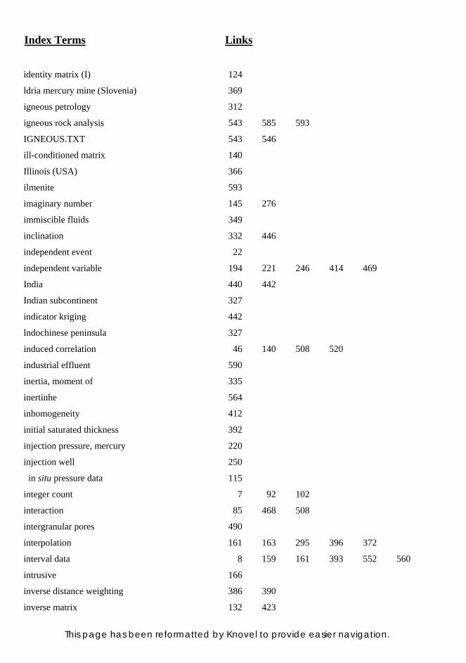
Index Terms Links
This page has been reformatted by Knovel to provide easier navigation.
identity matrix (I) 124
ldria mercury mine (Slovenia) 369
igneous petrology 312
igneous rock analysis 543 585 593
IGNEOUS.TXT 543 546
ill-conditioned matrix 140
Illinois (USA) 366
ilmenite 593
imaginary number 145 276
immiscible fluids 349
inclination 332 446
independent event 22
independent variable 194 221 246 414 469
India 440 442
Indian subcontinent 327
indicator kriging 442
lndochinese peninsula 327
induced correlation 46 140 508 520
industrial effluent 590
inertia, moment of 335
inertinhe 564
inhomogeneity 412
initial saturated thickness 392
injection pressure, mercury 220
injection well 250
in situ pressure data 115
integer count 7 92 102
interaction 85 468 508
intergranular pores 490
interpolation 161 163 295 396 372
interval data 8 159 161 393 552 560
intrusive 166
inverse distance weighting 386 390
inverse matrix 132 423

Index Terms Links
This page has been reformatted by Knovel to provide easier navigation.
inverse regression 205 217 205
iodine 97
ion exchange 575
Ireton shale (Upper Devonian) 404
iron (Fe) 167 265 287 411 448 486 590
Island Creek Shale (Missourian) 557
isopach map 372 395 449
Istrian peninsula 30 33 97 101 146 150
ISTRIA.TXT 146 152
ITALNAVY.TXT 11 6
IUGS Geochemical Map of the World 366
J
Jaccard’s coefficient 490
Japan 178
Java Sea 113
Jay Field (oil), Alabama-Florida, USA 285
joint probability 22 169 480 553 555 562
joints 313
Jurassic 220 285 591
K
Kaiser’s varimax (factor rotation) 533
KANSALT.TXT 154
Kansas (USA) 35 39 91 110 113 118 153
223 243 260 301 350 392 395
398 406 431 435 438 447 451
485 556 581
karst 444
KENTUCKY.TXT 464 470
Kentucky (USA) 271 463
Kepler, Johannes 266
kerogen 282 564

Index Terms Links
This page has been reformatted by Knovel to provide easier navigation.
key landmark 357
kite diagram 319
k-means procedure 499
Kolmogorov-Smirnov statistic 107 112 184
kriging 255 265 295 390 416 452
- block 437
- disjunctive 442
- error variance 418 420 424 432 442
- exact interpolator 418 427
- indicator 442
- multigaussian 442
- ordinary 420 432 437 440 452
- punctual 437
- simple 418 430
- universal 428 443
Kruskal-Wallis test 105
K2O (potassium) 48 114 202 486 570
kyanite 288
Kyushu (Japan) 178
L
La Chapelle bank (UK) 114
lack of fit 198 211 228 413
lag 244 248 417
lagoon, coastal 589
Lagrange multiplier 420 429 432
Laguna Mountains (Arizona) 446
lake deposit 278 285
Lambert projection (Schmidt net) 338 446
Lamont sandstone’ (Mississippian) 380 388
LAMONT.TXT 380 388
landmark 357 360 447 587
Landsat 327 593
landscape, equilibrium 283

Index Terms Links
This page has been reformatted by Knovel to provide easier navigation.
landslide 178
Lane Shale (Missourian) 557
Lansing-Kansas City Group (Pennsylvanian) 395 398 407
Laplace’s problem 296
Laramie Range (Wyoming) 153 279
large-sample statistics 68
Larrea tridentata (creosote bush) 445
latent factor (factor analysis) 527
latent value (See eigenvalue.)
latent vector (See eigenvector.)
“law of proportionate effect” 101
lead (Pb) 97 101 448
lease tract 303
least squares 191 382 385 407 462
- piecewise linear 384
- piecewise quadratic (gridding procedure) 384
Leduc Formation (Devonian) 403
LEDUC.TXT 371 406 411
level of significance 62
leveling (time series) 276
Ligonodina (conodont) 364
likelihood 12
Lilliefors procedure 109
limestone 88 127 160 168 172 220 243
444 581
line power spectrum 270 275
lineament 313 326
linear:
- drift 259 429 433
- interpolation 163
- projection (gridding) 385
- regression 199 203 273 283 288 464
- semivariogram model 261 435
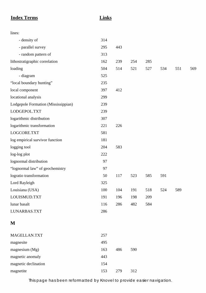
Index Terms Links
This page has been reformatted by Knovel to provide easier navigation.
lines:
- density of 314
- parallel survey 295 443
- random pattern of 313
lithostratigraphic correlation 162 239 254 285
loading 504 514 521 527 534 551 569
- diagram 525
“local boundary hunting” 235
local component 397 412
locational analysis 299
Lodgepole Formation (Mississippian) 239
LODGEPOL.TXT 239
logarithmic distribution 307
logarithmic transformation 221 226
LOGCORE.TXT 581
log empirical survivor function 181
logging tool 204 583
log-log plot 222
lognormal distribution 97
“lognormal law” of geochemistry 97
logratio transformation 50 117 523 585 591
Lord Rayleigh 325
Louisiana (USA) 100 104 191 518 524 589
LOUISMUD.TXT 191 196 198 209
lunar basalt 116 286 482 584
LUNARBAS.TXT 286
M
MAGELLAN.TXT 257
magnesite 495
magnesium (Mg) 163 486 590
magnetic anomaly 443
magnetic declination 154
magnetite 153 279 312

Index Terms Links
This page has been reformatted by Knovel to provide easier navigation.
MAGNETIT.TXT 153
Mahalanobis’ distance 478 574 588
major:- axis (principal axis) 215
- diagonal (of matrix) 124
- oxide 51 117 547
- product matrix 130 503 566
manganese (Mn) 164 590
Mann-Whitney test 103
MANOVA (multivariate analysis of variance) 487 592
Manticoceras (goniatite ammonoid) 502
map 293 300 311 338 344 354 370
405 417 442 452 593
- derivative 396
- drift 437
- error 425
- fault 393
- generalized derivative 396
- isopach 391 395 449
- kriging 417 428 435 442
- standard error 425 437
- trend residual 397 399 404 412 438 451
- of water-table elevation 422 427 431 437 440
mapping, plane-table 374
marginal probability 170 175 553
MARINEOL.TXT 591
marine sediment 591
marine seismic survey 256 263
Markov chain 161 168
- embedded 173
Markov property, first-order 172
Maryland (USA) 251 253
matrix:
- algebra 123 194 500
- cophenetic values 492

Index Terms Links
This page has been reformatted by Knovel to provide easier navigation.
matrix: (Cont.)
- correlation 147 466 492 499 509 517
- covariance 474 484 500 509 519 523 568
584
- diagonal 124
- distance 490 493 499 548
- elements of 123
- filter 395
- identity (I) 124
- ill-conditioned 140
- inverse 132 423
- major product 130 503 506
- minor product 130 503 505 566
- off-diagonal, elements of 124
- order of 124
- orthonormal, columns of 503 507
- overdetermined 520
- pooled variance-covariance 473 584 588
- rank of 145 505
- reproduced correlation 532 537
- residual correlation 533 537
- scalar 124
- similarity 488 491 499 540
- singular 132 139 145 152 425 502 523
- sparse 136
- square 124
- standardized variance-covariance 531 583
- symmetric 124
- transition 127 168 173
- tridiagonal 230
- unit 124
- variance-covariance 477 482 509 515 524 529 569
578 584 586
- within-groups covariance 573 576

Index Terms Links
This page has been reformatted by Knovel to provide easier navigation.
maturity 564
maximum likelihood factor analysis 528 538
MDS (multidimensional scaling) 560
- loadings 561 564
mean 33 61 66 72 192 202 276
306 355
- deviation 35
- direction 319 322 326 332 341 446
- rate of occurrence 179
- resultant 321 325 327 330
- square 80 369 409 197 469
measurement 7
median 32 103
median grain size 472 521
Mediterranean Sea 116
megacyclothem 556
meltwater 77
mercury (Hg) 220 369 448
- displacement 115 220 285
Merriam Limestone (Missourian) 557
metamorphism 592
Mexico 116 411 589
Mg (magnesium) 163 486 590
Michigan Basin (USA) 397
microfossil 553
microlaterolog 583
microparticle 77
microprobe 411
Midland Basin (Texas) 445
MIDLAND.TXT 173
Midland Valley (Scotland) 173
Milankovitch cycle 274
mine 156 265 280 287 366 437 439
590

Index Terms Links
This page has been reformatted by Knovel to provide easier navigation.
mineralogy, normative 593
minor product matrix 130 503 505 566
Miocene 282
misclassification ratio 476
Mississippian 153 239 380 388 593
Mississippi Delta 518
Mississippi River Valley 84
Missourian 556
mixed-effects model 83
Mn (manganese) 164 590
mode 34
moisture 191 198 211
moment of inertia 335
Montana (USA) 281
Monterey Formation (Miocene) 282
montmorillonite 281
monzonite 548
MOONCRST.TXT 116
Mt. Gleason, California (USA) 284
moving average 246 273 383
Mowry Shale (Cretaceous) 190 281
MOWRY.TXT 281
mud 191 198
- drilling 279
mudstone 174
multidimensional scaling (MDS) 548 552 560
multigaussian kriging 442
multigroup discriminant analysis 572 592
multinomial distribution 20
multiple correlation coefficient (R) 195 402
multiple regression 400 462 479 577
multiplicative model 223
multiplicative rule of probability 22
multivariate analysis of variance (MANOVA) 574 592

Index Terms Links
This page has been reformatted by Knovel to provide easier navigation.
multivariate morphometrics 357
multivariate normal 480 483 486 584 527 590
Muncie Creek Shale (Missourian) 557 560
Murray pluton (Canada) 446
mutually highest similarities 490 493
N
Na (sodium) 48 486 591
Naga Hills 327
National Earthquake Information Center 449
National Geophysical Data Center 446
natural end condition 230
natural neighbor 377
nearest neighbor 310 376 387 445 449
negative binomial 17 307
negative thickness 393
neighborhood 256 258 383 388 418 428 433
nested ANOVA 88 118 366 448 452
NESTED.TXT 88
neutron density 49 214
Nevada Test Site 588
Nevada (USA) 588 593
New Zealand 449
nickel 39
Noland County (Texas) 304
nominal data 7 93 103 161 393 549 552
nonnegative definite (semivariogram model) 261
nonparametric statistics 102
nonstationary 214 246 264 428 436
norite 548
normal distribution 27 34 36 55 69 75 92
109 111 227 246 322 341 355
412 424 435 477 479 538
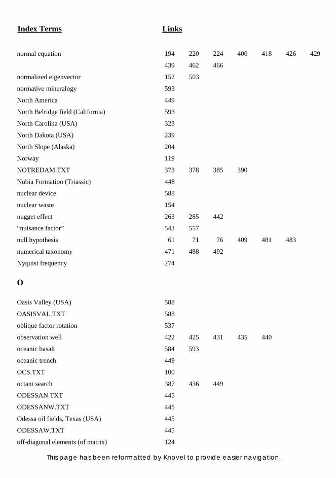
Index Terms Links
This page has been reformatted by Knovel to provide easier navigation.
normal equation 194 220 224 400 418 426 429
439 462 466
normalized eigenvector 152 503
normative mineralogy 593
North America 449
North Belridge field (California) 593
North Carolina (USA) 323
North Dakota (USA) 239
North Slope (Alaska) 204
Norway 119
NOTREDAM.TXT 373 378 385 390
Nubia Formation (Triassic) 448
nuclear device 588
nuclear waste 154
nugget effect 263 285 442
“nuisance factor” 543 557
null hypothesis 61 71 76 409 481 483
numerical taxonomy 471 488 492
Nyquist frequency 274
O
Oasis Valley (USA) 588
OASISVAL.TXT 588
oblique factor rotation 537
observation well 422 425 431 435 440
oceanic basalt 584 593
oceanic trench 449
OCS.TXT 100
octant search 387 436 449
ODESSAN.TXT 445
ODESSANW.TXT 445
Odessa oil fields, Texas (USA) 445
ODESSAW.TXT 445
off-diagonal elements (of matrix) 124

Index Terms Links
This page has been reformatted by Knovel to provide easier navigation.
offshore sand bar 371 472 474 476
Ohio (USA) 380 388
oil:
- field 31 36 97 100 220 285 305
327 355 393 403 412 439 445
449 451 593
-shape of 355
- volume 100
- gravity 282 410
- heavy 282
- production decline curve 592
- reservoir 239 392
- saturation 36 392 581 583
- shale 278 285
- well 14 301 385 449 589
Oklahoma (USA) 36 99 211 225 391 406 575
OKLA.TXT 211
Oligocene 284 444 593
olivine 153 279 594
one-tailed test 63 71 108 187 213
one-way analysis of variance (ANOVA) 78 117 572 589
ONEOVA.TXT 79
Ontario (Canada) 364 446
operational taxonomic unit, OTU 489
opisthoparian (trilobite) 587
ordered measurements 592
order of matrix 124
ordinal data 8 93 103 106 161 549 552
560
ordinary kriging 420 432 437 440 452
ordinary regression 217 284
ordination 239
ORDNALBX.TXT 562
Ordovician 84 301 357 447 451

Index Terms Links
This page has been reformatted by Knovel to provide easier navigation.
oreodont 284
OREODONT.TXT 284
organic material 566 591
orientation 316 321 329 340
orthid brachiopod, Resserella sp. 357 447 587
ORTHID.TXT 359 447 587
orthogonal axes 150 511 515 533
orthogonal regression 218
orthonormal (columns of matrix) 503 507
orthoquartzite 84
ostracode 360
Ouachita Mountains (USA) 391
Outer Continental Shelf 100
outlier 116
overdetermined matrix 520
oxide, major 51 117 547
oxygen isotope ratio (δ18O) 273 591
Ozark Dome (USA) 397
P
Pacific Ocean 364 451 584 594
PAGELER.TXT 243
pair-group methods (clustering) 496
Paleocene 119
paleocurrent 326
paleoecology 553 557
paleogeography 372
Paleolithic 366
Paleozoic 211
Paola Shale (Missourian) 557
parabola 402
parallel-line search 295 443
partial correlation (factor analysis) 527 531
partial regression coefficient 409 463 465

Index Terms Links
This page has been reformatted by Knovel to provide easier navigation.
partitioning methods (classification) 488
pattern recognition 162 271
PCA (See principal component.)
PCOORD.TXT 551
Pearce element ratio diagram 48
Pearsonian correlation coefficient 105 116
pebbles 46 75 126 490
pedicle valve 357
pegmatite 188
Pennsylvanian 35 39 70 73 113 115 243
366 391 395 398 407 581 583
percentile 32
perimeter 355 359 448
period 267 353
periodogram 161 270 274 351
peristome 503
permeability 27 84 99 115 225 331 581
583 591
Permian 49 154 282 445 449
Permian Basin 304 309
Perth Amboy, New Jersey (USA) 284
Peru 451
Petrified Forest, Arizona (USA) 284
petrofabric 331 337 341 412 591
petroleum 99 113 566 591
- exploration 414 451
- source-rock 564
petrophysical well log 102 115 154 204 583
“phantom black shale” 560
phase angle 267 362
phi transformation 97
Phillippines 439
phillipsite 592
phosphate 118
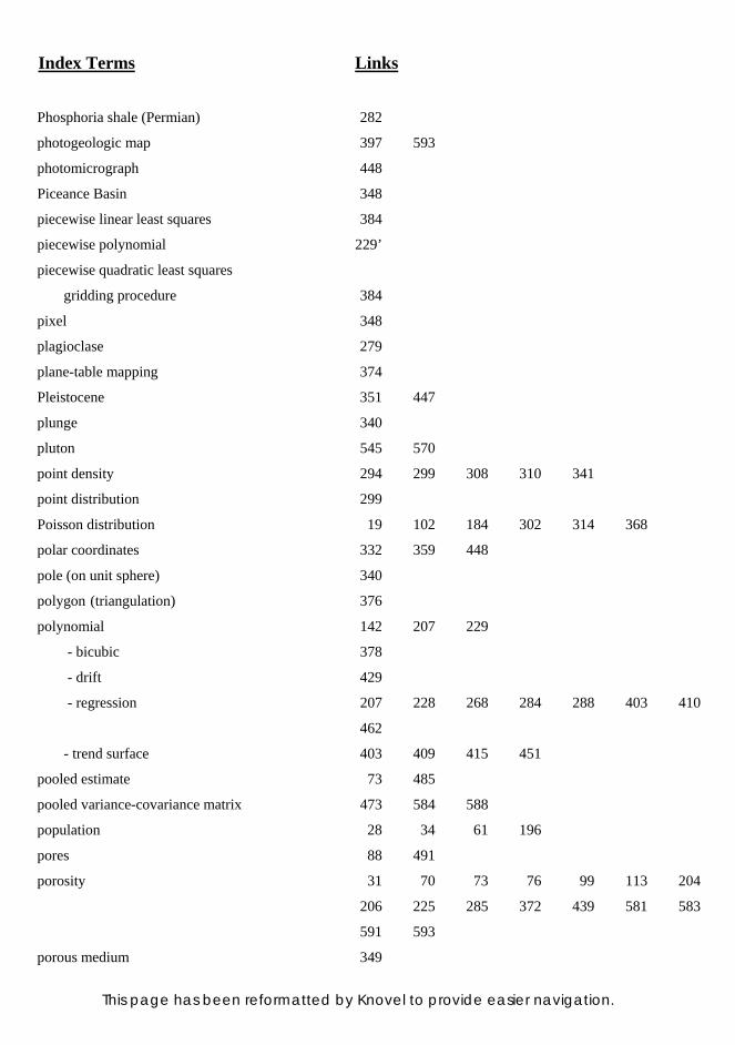
Index Terms Links
This page has been reformatted by Knovel to provide easier navigation.
Phosphoria shale (Permian) 282
photogeologic map 397 593
photomicrograph 448
Piceance Basin 348
piecewise linear least squares 384
piecewise polynomial 229’
piecewise quadratic least squares
gridding procedure 384
pixel 348
plagioclase 279
plane-table mapping 374
Pleistocene 351 447
plunge 340
pluton 545 570
point density 294 299 308 310 341
point distribution 299
Poisson distribution 19 102 184 302 314 368
polar coordinates 332 359 448
pole (on unit sphere) 340
polygon (triangulation) 376
polynomial 142 207 229
- bicubic 378
- drift 429
- regression 207 228 268 284 288 403 410
462
- trend surface 403 409 415 451
pooled estimate 73 485
pooled variance-covariance matrix 473 584 588
population 28 34 61 196
pores 88 491
porosity 31 70 73 76 99 113 204
206 225 285 372 439 581 583
591 593
porous medium 349

Index Terms Links
This page has been reformatted by Knovel to provide easier navigation.
PORPERM.TXT 99 225
positive definite (semivariogram) 261
postmultiplication 129
potassium (K2O) 48 114 202 486 570
potassium-40 243
power 271 352 365 415
- plant 444
- spectrum 270 277 362 364 447 592
- two-dimensional 354
- transform 102
Precambrian 116 279 397
precision 26
premultiplication 129
primate 357
principal axis 215 511 537
principal component:
- analysis (PCA) 235 239 470 479 507 509 527
540 566 569 577 588 592
- loading 513 517 525
- score 512 519 522 526 535 556 589
principal coordinates 507 548 567
principal diagonal 124
prism 277
pristane/n-C17 ratio 564
pristane/phytane ratio 564 591
probabilistic similarity coefficient 490
probability 11 127 560
- additive rule of 21
- bivariate normal distribution 481
- conditional 22 169 552
- discrete 12
- distribution, normal (See normal distribution.)
- ellipses, bivariate 447
- geometric 295

Index Terms Links
This page has been reformatted by Knovel to provide easier navigation.
probability (Cont.)
- joint 22 169 480 553 555 562
- marginal 170 175 553
- multiplicative rule of 22
Procrustes analysis 357
profile data 592
profile distance 560 563
PROFILE.TXT 592
projection equation 338
proper value 141
proper vector 141
prospects (oil and gas) 104 593
PROSPECT.TXT 154
provenance 364
Prudhoe Bay oil field (Alaska) 204
PRUDHOE.TXT 204
pseudo landmark 357
pseudopoint (triangulation) 380
P2O5 116
punctual kriging 437
pure error 198 211
P-value 64
pygidium (of trilobite) 587
pyroxene 51 54
Pythagorean theorem 320 335 383
Q
Q-mode:
- analysis 500 505
- factor analysis 521 540
- loading 543 560 566 568
- score 504 556 568
QMODE.TXT 541

Index Terms Links
This page has been reformatted by Knovel to provide easier navigation.
quadrant search 387
quadrat 300 302 445
quadratic equation 142 209 259 287 400
quantile 32
quartile 32
quartz 114 116 188 446 490 594
- diorite 548
- monzonite 570
- syenite 548
QUEBECAU.TXT 278
Quebec (Canada) 278
Quindaro Shale (Missourian) 557
R
radian 266 325
radiation 30 33 444 570
radioactivity 243 366 404
radiolarian 189
radionuclide 570
RADIO.TXT 570
random-effects model (Model II) 83
random:
- error 196 199 227 412 462
- function (geostatistics) 417
- location 299 302 312
- noise 246
- order 515
- sample 28 408 483
- variable 25 79 196 246 516
- walk 315
randomness, testing for 322 341
range (geostatistics) 256 433
Rangely oil field (USA) 115
RANGELY.TXT 115

Index Terms Links
This page has been reformatted by Knovel to provide easier navigation.
Raniganj coal field (India) 440
RANIGANJ.TXT 440
rank of matrix 145 505
rank of observations 8 103 514
Rappahannock, Virginia (USA) 284
rate of occurrence (of events) 184
ratio scale 8 159 161 393 552 560
Raton Basin (Colorado) 396
Rayleigh’s test 325
Raytown Limestone (Missourian) 557 560
reaction rim 286
Recent (Holocene) 162 191 273
reciprocal matrix (See inverse matrix.)
rectangular integration 166
recursive procedure 237 242
reduced major axis (RMA) 214 217 284
reef 371 403 449
REEF.TXT 449
regional dip 398 404
regionalized variable 254 295 416 420 428 433
regression 161 191 269 284 295 346 352
397 462 590
- “best possible” 468
- curvilinear 207
- generalized linear 417
- inverse 204
- ordinary 217 284
- orthogonal 218
- through the origin 220
“reification” 517
relaxed end condition 230
remanent magnetism 446
remote sensing 444 593
replicate 35 78 199 413 425

Index Terms Links
This page has been reformatted by Knovel to provide easier navigation.
reproduced correlation matrix 532 537
R.V. Glomar Challenger 446
RESENG.TXT 83
reserve estimates (coal) 441
reservoir, oil 239 392
residual 226 398 401 405 408 428 433
437
- correlation matrix 533 537
- map 406
- matrix (maximum likelihood) 539
- stationary 428
- trend map 451
resin 564
resistivity 114 239
response surface 412
Resserella sp. (brachiopod) 357 447 587
RESSEREL.TXT 358 447 587
resultant 319 325 327 329 332 341
rhodochrosite 495
rhyolitic volcanic ash 281
Rice County, Kansas (USA) 113 154
Richardson’s dimension 346
river 283 463 467 469
RMA line 215
R- mode:
- analysis 500 504 509 566
- correspondence axis 556
- factor analysis 526 542
- loading 504 556 560 562 568
- score 504 506 535 566
R, multiple correlation coefficient 195 402
rock analysis, igneous 543 585 593
Rock-Eval pyrolysis 119 593
Rock Lake Shale (Missourian) 557

Index Terms Links
This page has been reformatted by Knovel to provide easier navigation.
Rocky Mountain Arsenal (Colorado) 250
Rocky Mountains (USA) 189 250 278 285 403
rose diagram 316 323 329 446
rotation, factor 533 545
roughness (fractal analysis) 342 353 363
round-off error 209
roundness 106
R- and Q-mode analysis 501 566
ruler method (fractal analysis) 343
runoff 271 589
runs test 161 185 278
S
St. Peter Sandstone (Ordovician) 84
salinity 93 96 111 251 253
salt dome 100 104
saltwater 575 589
sample, definition of 28
sample, random 29 486
sample size (trend-surface analysis) 415
sampling 6 20 28 315 368 486
San Andres Limestone (Permian) 445
sand 116 140 351 355 359 362 371
403 446 472 520 570 572 589
Sandford St. Martin (UK) 285
sandstone 78 81 106 114 119 127 160
168 172 211 348 397 593
SANDS.TXT 472 474
San Jacinto County (Texas) 282
Santa Barbara Channel 282
Santa Maria basin (California) 282
satellite image 327 444 593
saturated thickness 393
saturates 564

Index Terms Links
This page has been reformatted by Knovel to provide easier navigation.
scalar matrix 124
Schellerhau pluton 48 117
SCHELLER.TXT 48 117
Schmidt net (Lambert projection) 338 446
Scotland 107 173
sea level, changes in 557
search:- for control points 263 383 387 394
- nearest-neighbor 387 449
- octant 387 449
- pattern 294 443
- quadrant 387
- systematic 294
seawater 251 556
secondary dolomitization 591
second derivative 229 396
second-order Markov (sequence) 172
second-order stationarity (time series) 276
sediment 114 116 283 369 404 518 589
sedimentary zeolites 114 592
sediment grain size 114 116 472 518 589 592
sediment load 283
segmenting sequences 234
seismic reflection 256 288 296 370 380 388 390
444 449 452
SEISMIC.TXT 449 452
selenium 97
self-affine 342
self-similar 243 342 346
self-stationary 276
semiaxis 147 152 511
semimadogram 264
semivariance 254 420 422 426 431 433 439
Index Terms Links
This page has been reformatted by Knovel to provide easier navigation.
semivariogram 161 255 259 287 417 422 428
431 433 436 452 590
- alternatives to 264
- converting to covariogram 265
- experimental 255 260 264 285 422 452
- Gaussian 262 442
- linear 261 422 431 434
- span of 285
- spherical 261 263 436
- theoretical 255 419 421
sequence 159
serial correlation 182 245
seriation 161 239
series of events 161 178
serpentinite 593
shale 35 38 49 69 127 154 160
168 172 189 243 281 366 403
563 565 591 593
- black 281 366
- oil 278 285
- “phantom black” 560
- siliceous 90 189 281
shape 355 448 587
sharpening filter 395
shear stress 155 284
shingle beach 46 75
sialic rock 545
siderite 287 495
Siegel-Tu key test 105
Sierpinski gasket (fractal analysis) 343
significance 64
- level of 62
- tests of 71 74 76 82 86 89 96

Index Terms Links
This page has been reformatted by Knovel to provide easier navigation.
significance (Cont.)
106 187 197 202 210 224 307
323 342 407 465 468 477 482
484 487 580 584
significant digits 466
silica (SiO2) 486 590 594
siliceous shale 90 189 281
siliciclast 448
sill 256 258 261 436 442
sill, diabase 446
silt 116 520
siltstone 119 174 211
similarities, mutually highest 490 493
similarity:
- cosine θ 540
- mutually highest 493
- within-cluster 498
- fractal dimension 343
- matrix 488 500 540 554 560 562
simple kriging 418 430 437
simple matching coefficient 490
simple structure 531 540
simplex 523
simulation, conditional 443
simultaneous equation 132 194 209 400 428 470 502
simultaneous R- and Q-mode analysis 566
sine wave 246 268
single linkage clustering 496
singular matrix 132 139 145 152 425 502 523
singular value 503 528 541 555 568 592
singular value decomposition (SVD) 136 152 502 531 556 569 573
578
singular value 503 528 541 555 568 592
sinkhole 444

Index Terms Links
This page has been reformatted by Knovel to provide easier navigation.
sinusoidal (wave form) 268 274
SiO2 (silica) 486 590 594
64-Zone sandstone (Oligocene) 593
SLOFEPB.TXT 448 452
slope 283 384 396 449
slotting 239
Slovenia 369 448
SLOVENIA.TXT 369 448 452
Smackover Formation (Jurassic) 285 591
S MACKOVR .TXT 285
small-sample statistics 68
smithsonite 495
smoothing (filtering) 395
snow 273
social sciences 501 552
sodium (Na) 48 486 591
soil 97 101 146 235 285 351 444
448
solvent extraction 564
Solway Lowlands (UK) 117
sonic transit time 49 154 204 206 214 285 288
581 583
SONIC.TXT 288
Sonora area (Mexico) 589
SONORA.TXT 589
sorting, degree of 106 521
source rock 566 591
South Africa 397
South America 256 263 450
South Bend Limestone (Missourian) 557
span (semivariogram) 285
span (spline function) 229
sparse matrix 136
spatial covariance 417 430 433 439 443 452

Index Terms Links
This page has been reformatted by Knovel to provide easier navigation.
spatial domain 277 396
Spearman’s rank correlation 106 116
specific gravity 113 279
spectral:
- analysis 266 287 351 590
- density 161 272
- method (fractals) 351 447
- window (filter) 273
spectrum, Fourier 270 272 353 359 361 364 447
sphalerite 411
SPHALRT.TXT 411
spherical:
- angle 333
- data 330 446
- model (semivariogram) 261 435
- variance 332 334 446
Spiro Sand (Pennsylvanian) 391
Spitzbergen Island 119
spline function 161 228 378
Spring Hill Limestone (Missourian) 557
SPTZBRGN.TXT 119
spurious negative correlation 48
squared Euclidean distance 548
square matrix 124
square network 312
square-root transformation 102
Sr 591
stagewise regression 469
standard deviation 35 216 465
standard error 59 67 201 203 218 306 314
325 364 424 435 452
standardization 57 61 418 477 493 495 517
519 528
standardized variance-covariance matrix 531 583

Index Terms Links
This page has been reformatted by Knovel to provide easier navigation.
standard normal form 57 466
stationarity, first-order (time series) 276
stationarity, second-order (time series) 418
stationarity, strong 276
stationary:
- data 183 214 256 279 447
- probability matrix 131
- residual 428
statistics 29 34 479 482
- large- and small-sample 68
stepwise discriminant analysis 479
stepwise regression 469
stereographic projection (Wulff net) 338
stochastic 274 342 349
Stoner Limestone (Missourian) 557 560
STPETER.TXT 84
Straits of Magellan 256 263
stratigraphic correlation 162 254
stratigraphic section 168 239
stratovolcano 179
stream 163 283 351 390 464 468
- basin 283
- profile 592
- sediment analysis 590
stress 155
“stretchability” 147
Striation 316 325
strike and dip 331
strip mine 366
strong stationarity 276
strontianite 494
structural analysis 218 259 422 429 434
structural data 370 394 398 405 412
Student’s t 68 482

Index Terms Links
This page has been reformatted by Knovel to provide easier navigation.
subcomposition 50 591 594
subduction surface 202 449
submarine canyon 283
submarine fan 283 593
subsurface structural data 380 388 391 398 404
sulfur 282 591
SULFUR.TXT 282
sum of squares 37 43 45 79 86 195 197
205 210 216 236 270 401 408
465 467 473 497
sunspot cycle 279
support (of regionalized variable) 255 437
surface-wave dispersion curve 592
surveying 374
Sweden 590
SWEDEN.TXT 590
syenite 548
symmetric matrix 124
systematic error 79
T
TABLE612.TXT 510 514
tally 168 553
tangent plane 339
target 296
taxonomy, numerical 487
t-distribution 68 480
tectonic plate 446
temperature 8 281 411 446
- bottomhole 153
TEMPER.TXT 282
Tensleep Sandstone (Pennsylvanian) 70 72 76
tensor 378
Tertiary 287 348 397

Index Terms Links
This page has been reformatted by Knovel to provide easier navigation.
Tertiary basin (Wyoming) 397
tests of significance (See significance, tests of.)
Texas (USA) 100 282 304 309 406 445 449
472 575
textural maturity 106
Thames River valley (UK) 235
THEMATIC.TXT 593
theoretical semivariogram 255 419 421
“theory of breakage” 101
thermal maturity 281 593
thermal radiation 445
THERMAL.TXT 444
thickness, negative 393
thickness, saturated 391
Thiessen polygon 376
thin section 88 490
thorium 570
tidal cycle 251
time domain 277
time series 159 178 185 213 243 250 266
275 295 417
TIN (triangulated irregular network) 375 393
titanium 48
tolerance limit 219
Tonga-Kermadec Trench (New Zealand) 449
TONGA.TXT 449
topographic data 351 370 373 378 50 383 386
topography, “basket-of-eggs” 117
topologic information 375
TOPSOIL.TXT 285
torus 311
total organic carbon (TOC) 119 564
total regression coefficient 463
total sum of squares 80 195

Index Terms Links
This page has been reformatted by Knovel to provide easier navigation.
township (U.S. Public Land Survey system) 366
trace element 146 588
trace of matrix 150 512 524 551
tracts (containing discovery wells) 305 309
transient 287
transition matrix 127 168 173
transition pair 178
transposition 126
trapezoidal approximation 360
tree diagram( See dendrogram)
trend:
- in observations) 161 179 182 198 213 281
- residual map 451
- surface 195 294 378 384 397 429 449
451 462 465 479 589
- edge effects in 391 415
triangular diagram 49
triangular network, Delaunay 375
triangulated irregular network (TIN) 375 393
triangulation 374 388 449
Triassic 448
triaxial stress 284
tridiagonal matrix 230
trigonometric relationship 266
trilobite 586
TRILOBIT.TXT 586
truncation 44
T2 test 474 482 487
t-test 70 74 116 212 250 307 480
Tukey-Hanning filter 273
two-tailed test 63 108 187 213
two-way analysis of variance (ANOVA) 84 116
two-way travel time 449 452
TWOWAY.TXT 115

Index Terms Links
This page has been reformatted by Knovel to provide easier navigation.
Tyne Gap (UK) 117
type I error 62
type II error 62 415
U
ultimate production 98
ultrabasite 288
ukramafic 280
umbilicus 502
unbalanced design (ANOVA) 367
unbiased estimate 34 192 418 429
unconditional 170
unconformity (stratigraphic) 388
underlying (latent) factor 527
uniform density 29
uniform distribution 301 323 337
unimodal vector 337
unique factor 527
unique variance 507 536
U.S. Geological Survey 351 366
U.S. Gulf Coast 191
unit matrix 124
unit vector 319
universal kriging 428 443
Universal Transverse Mercator (UTM) projection 369 435 452
University of Sonora (Mexico) 589
unweighted average linkage 497
uranium 570
“Useful Heat Value” (UHV) 440
Utah (USA) 439 586 593
UTM coordinates 369 435 452
V

Index Terms Links
This page has been reformatted by Knovel to provide easier navigation.
vanadium 39
variable:- continuous 8 25
- dependent 194 400 462 464 577
- discrete 7 12 490
- independent 194 221 246 414 469
- random 25 196 254 416
- regionalized 254 295 416 420 428 433
- regressed 194
- regressor 194
variance 35 66 69 75 94 101 195
226 270 276 306 311 355 361
398 407
variancecovariance matrix 477 482 509 515 524 529 569
578 584 586
variation, coefficient of 39
varimax factor score 547
varimax rotation 534
varve 273 279 285
vector 124
- direction 316 445
- fixed probability 170 173
- latent (See eigenvector.)
- proper 141
- resultant 319 445 450
vegetation, distribution of 444
Vilas Shale (Missourian) 557
vineyard 146 150
Viola Limestone (Ordovician) 575
Virginia (USA) 570
viscous fingering 349
vitrinite reflectance 564 593
volcanic ash, rhyolitic 281
volcanic eruption 178 202
von Mises distribution 322 324 341

Index Terms Links
This page has been reformatted by Knovel to provide easier navigation.
Voronoi polygon 376
W
Wabaunsee County (Kansas) 244
Wales 284
Ward’s method 238 497
Wasatch Formation (Eocene) 348 446
WASATCH.TXT 446
waste, injected 250
water:
- connate 575
- quality 485 588
- saturation 581 583
- table 91 223 260 422 424 431 434
water-flood breakthrough 445
WATER.TXT 91
“Waulsortian” (carbonate algal) mound 239
wavelength 267
wave number 267 352 362
weak stationarity (time series) 276
Weber Sandstone (Pennsylvanian) 115
Weichselian (Wisconsinan) glacial period 274
weighted- averaging 382 395 389 449
- pair-group linkage 493 496 546
- projection 384 390
- regression 224
Wellington Formation (Permian) 49 154
well-log analysis 227 581
well-log density 23
well logs, automatic zoning of 234
well, oil 14 301 385 449 589
well, water 422 485 588
WELLWATR.TXT 486
West Lyons oil field (Kansas) 113

Index Terms Links
This page has been reformatted by Knovel to provide easier navigation.
West Texas (USA) 36
WHITE.TXT 93
Whitewater Bay 93 96 111
whorl 502
Wilburton gas field (Oklahoma) 391
Wilcoxon test 105
Williston Basin (North Dakota) 239
Windfall Reef (Devonian) 406
Wind River Basin 73
Wisconsinan 274
Wishart’s modification 498
witherite 494
within-cluster similarity 498
within-groups covariance matrix 573 576
WLYONS.TXT 113
Wolf River (Kansas) 350
Woodford shale (Devonian) 282
Wulff net 338 446
Wyoming (USA) 70 72 125 153 279 286 397
406 446
X
xenocryst 286
Xian province (China) 113
X-ray fluorescence 206
Y
Yellowcraigs (Scotland) 108
Yuma (Arizona) 446
YUMA.PIC 447
YUMA.TIF 447
Z

Index Terms Links
This page has been reformatted by Knovel to provide easier navigation.
zeolites, sedimentary 114 592
ZEOLITES.TXT 592
zero isopach problem 391 449
zircon 102
zonation 234
z-score 57 95 110 476
z-statistic 57 61 63 66 310