statistical theory - pomona...

Statistical Theory

Lecture Notes

Adolfo J. Rumbosc⃝ Draft date December 18, 2009

Contents

1 Introduction 51.1 Introduction to statistical inference . . . . . . . . . . . . . . . . . 5

1.1.1 An Introductory Example . . . . . . . . . . . . . . . . . . 51.1.2 Sampling: Concepts and Terminology . . . . . . . . . . . 7

2 Estimation 132.1 Estimating the Mean of a Distribution . . . . . . . . . . . . . . . 132.2 Interval Estimate for Proportions . . . . . . . . . . . . . . . . . . 152.3 Interval Estimates for the Mean . . . . . . . . . . . . . . . . . . . 17

2.3.1 The �2 Distribution . . . . . . . . . . . . . . . . . . . . . 182.3.2 The t Distribution . . . . . . . . . . . . . . . . . . . . . . 262.3.3 Sampling from a normal distribution . . . . . . . . . . . . 292.3.4 Distribution of the Sample Variance from a Normal Dis-

tribution . . . . . . . . . . . . . . . . . . . . . . . . . . . 332.3.5 The Distribution of Tn . . . . . . . . . . . . . . . . . . . . 39

3 Hypothesis Testing 433.1 Chi–Square Goodness of Fit Test . . . . . . . . . . . . . . . . . . 44

3.1.1 The Multinomial Distribution . . . . . . . . . . . . . . . . 463.1.2 The Pearson Chi-Square Statistic . . . . . . . . . . . . . . 483.1.3 Goodness of Fit Test . . . . . . . . . . . . . . . . . . . . . 49

3.2 The Language and Logic of Hypothesis Tests . . . . . . . . . . . 503.3 Hypothesis Tests in General . . . . . . . . . . . . . . . . . . . . . 543.4 Likelihood Ratio Test . . . . . . . . . . . . . . . . . . . . . . . . 613.5 The Neyman–Pearson Lemma . . . . . . . . . . . . . . . . . . . . 73

4 Evaluating Estimators 774.1 Mean Squared Error . . . . . . . . . . . . . . . . . . . . . . . . . 774.2 Cramer–Rao Theorem . . . . . . . . . . . . . . . . . . . . . . . . 80

A Pearson Chi–Square Statistic 87

B The Variance of the Sample Variance 93

3

4 CONTENTS

Chapter 1

Introduction

1.1 Introduction to statistical inference

The main topic of this course is statistical inference. Loosely speaking, statisti-cal inference is the process of going from information gained from a sample toinferences about a population from which the sample is taken. There are twoaspects of statistical inference that we’ll be studying in this course: estimationand hypothesis testing. In estimation, we try to determine parameters from apopulation based on quantities, referred to as statistics, calculated from datain a sample. The degree to which the estimates resemble the parameters be-ing estimated can be measured by ascertaining the probability that a certainrange of values around the estimate will contain the actual parameter. The useof probability is at the core of statistical inference; it involves the postulationof a certain probability model underlying the situation being studied and cal-culations based on that model. The same procedure can in turn be used todetermine the degree to which the data in the sample support the underlyingmodel; this is the essence of hypothesis testing.

Before we delve into the details of the statistical theory of estimation andhypothesis testing, we will present a simple example which will serve to illustrateseveral aspects of the theory.

1.1.1 An Introductory Example

I have a hot–air popcorn popper which I have been using a lot lately. It is asmall appliance consisting of a metal, cylindrical container with narrow ventsat the bottom, on the sides of the cylinder, through which hot air is pumped.The vents are slanted in a given direction so that the kernels are made tocirculate at the bottom of the container. The top of the container is coveredwith a hard-plastic lid with a wide spout that directs popped and unpoppedkernels to a container placed next to the popper. The instructions call forone–quarter cup of kernels to be placed at the bottom of the container andthe device to be plugged in. After a short while of the kernels swirling in hot

5

6 CHAPTER 1. INTRODUCTION

air, a few of the kernels begin to pop. Pressure from the circulating air andother kernels popping an bouncing off around inside the cylinder forces kernelsto the top of the container, then to the spout, and finally into the container.Once you start eating the popcorn, you realize that not all the kernels popped.You also notice that there are two kinds of unpopped kernels: those that justdidn’t pop and those that were kicked out of the container before they couldget warm enough to pop. In any case, after you are done eating the poppedkernels, you cannot resit the temptation to count how many kernels did not pop.Table 1.1 shows the results of 27 popping sessions performed under nearly thesame conditions. Each popping session represents a random experiment.1 The

Trial Number of Uppopped Kernels1 322 113 324 95 176 87 78 159 139

10 11011 12412 11113 6714 14315 3516 5217 3518 6519 4420 5221 4922 1823 5624 13125 5526 5927 37

Table 1.1: Number of Unpopped Kernels out of 1/4–cup of popcorn

1A random experiment is a process or observation, which can be repeated indefinitelyunder the same conditions, and whose outcomes cannot be predicted with certainty beforethe experiment is performed.

1.1. INTRODUCTION TO STATISTICAL INFERENCE 7

number of unpopped kernels is a random variable2 which we obtain from theoutcome of each experiment. Denoting the number of unpopped kernels in agiven run by X, we may postulate that X follows a Binomial distribution withparameters N and p, where p is the probability that a given kernel will not pop(either because it was kicked out of the container too early, or because it wouldjust not pop) and N is the number of kernels contained in one-quarter cup. Wewrite

X ∼ binom(N, p)

and have that

P (X = k) =

(N

k

)pk(1− p)N−k for k = 0, 1, 2, . . . , N,

where (N

k

)=

N !

k!(N − k)!, k = 0, 1, 2 . . . , N.

This is the underlying probability model that we may postulate for this situa-tion. The probability of a failure to pop for a given kernel, p, and the number ofkernels, N , in one–quarter cup are unknown parameters. The challenge beforeus is to use the data in Table 1.1 on page 6 to estimate the parameter p. No-tice that N is also unknown, so we’ll also have to estimate N as well; however,the data in Table 1.1 do not give enough information do so. We will thereforehave to design a new experiment to obtain data that will allow us to estimateN . This will be done in the next chapter. Before we proceed further, we willwill lay out the sampling notions and terminology that are at the foundation ofstatistical inference.

1.1.2 Sampling: Concepts and Terminology

Suppose we wanted to estimate the number of popcorn kernels in one quartercup of popcorn. In order to do this we can sample one quarter cup from abag of popcorn and count the kernels in the quarter cup. Each time we dothe sampling we get a value, Ni, for the number of kernels. We postulate thatthere is a value, �, which gives the mean value of kernels in one quarter cup ofpopcorn. It is reasonable to assume that the distribution of each of the Ni, fori = 1, 2, 3, . . ., is normal around � with certain variance �2. That is,

Ni ∼ normal(�, �2) for all i = 1, 2, 3, . . . ,

so that each of the Nis has a density function, fN

, given by

fN

(x) =1√2��

e−(x−�)2

2�2 , for −∞ < x <∞.

2A random variable is a numerical outcome of a random experiment whose value cannotbe determined with certainty.


Hence, the probability that the number of kernels in one quarter cup of popcornlies within certain range of values, a ⩽ N < b is

P (a ⩽ N < b) =

∫ b

a

fN

(x) dx.

Notice here that we are approximating a discrete random variable, N , by acontinuous one. This approximation is justified if we are dealing with largenumbers of kernels, so that a few kernels might not make a large relative differ-ence. Table 1.2 shows a few of those numbers. If we also assume that the Nis

Sample Number of Kernels1 3562 3683 3564 3515 3396 2987 2898 3529 447

10 31411 33212 36913 29814 32715 31916 31617 34118 36719 35720 334

Table 1.2: Number of Kernels in 1/4–cup of popcorn

are independent random variables, then N1, N2, . . . , Nn constitutes a randomsample of size n.

Definition 1.1.1 (Random Sample). (See also [HCM04, Definition 5.1.1, p234]) The random variables, X1, X2, . . . , Xn, form a random sample of size n ona random variable X if they are independent and each has the same distributionas that of X. We say that X1, X2, . . . , Xn constitute a random sample from thedistribution of X.

Example 1.1.2. The second column of Table 1.2 shows values from a randomsample from from the distribution of the number of kernels, N , in one-quartercup of popcorn kernels.


Given a random sample, X1, X2, . . . , Xn, from the distribution of a randomvariable, X, the sample mean, Xn, is defined by

Xn =X1 +X2 + ⋅ ⋅ ⋅+Xn

n.

Xn is an example of a statistic.

Definition 1.1.3 (Statistic). (See also [HCM04, Definition 5.1.2, p 235]) Astatistic is a function of a random sample. In other words, a statistic is aquantity that is calculated from data contained in a random sample.

Let X1, X2, . . . , Xn denote a random sample from a distribution of mean �and variance �2. Then the expected value of the sample mean Xn is

E(Xn) = �.

We say that Xn is an unbiased estimator for the mean �.

Example 1.1.4 (Unbiased Estimation of the Variance). Let X1, X2, . . . , Xn bea random sample from a distribution of mean � and variance �2. Consider

n∑k=1

(Xk − �)2 =

n∑k=1

[X2k − 2�Xk + �2

]

=

n∑k=1

X2k − 2�

n∑k=1

Xk + n�2

=

n∑k=1

X2k − 2�nXn + n�2.

On the other hand,

n∑k=1

(Xk −Xn)2 =

n∑k=1

[X2k − 2XnXk +X

2

n

]

=

n∑k=1

X2k − 2Xn

n∑k=1

Xk + nX2

n

=

n∑k=1

X2k − 2nXnXn + nX

2

n

=

n∑k=1

X2k − nX

2

n.


Consequently,

n∑k=1

(Xk − �)2 −n∑k=1

(Xk −Xn)2 = nX2

n − 2�nXn + n�2 = n(Xn − �)2.

It then follows that

n∑k=1

(Xk −Xn)2 =

n∑k=1

(Xk − �)2 − n(Xn − �)2.

Taking expectations on both sides, we get

E

(n∑k=1

(Xk −Xn)2

)=

n∑k=1

E[(Xk − �)2

]− nE

[(Xn − �)2

]

=

n∑k=1

�2 − nvar(Xn)

= n�2 − n�2

n

= (n− 1)�2.

Thus, dividing by n− 1,

E

(1

n− 1

n∑k=1

(Xk −Xn)2

)= �2.

Hence, the random variable

S2n =

1

n− 1

n∑k=1

(Xk −Xn)2,

called the sample variance, is an unbiased estimator of the variance.

Given a random sample, X1, X2, . . . , Xn, from a distribution with mean �and variance �2, and a statistic, T = T (X1, X2, . . . , Xn), based on the ran-dom sample, it is of interest to find out what the distribution of the statistic,T , is. This is called the sampling distribution of T . For example, we wouldlike to know what the sampling distribution of the sample mean, Xn, is. Inorder to find out what the sampling distribution of a statistic is, we need toknow the joint distribution, F(X1,X2,...,Xn)(x1, x2, . . . , xn), of the sample vari-able X1, X2, . . . , Xn is. Since, the variables X1, X2, . . . , Xn are independentlyand identically distributed (iid), then we can compute

F(X1,X2,...,Xn)(x1, x2, . . . , xn) = FX(x1) ⋅ FX(x2) ⋅ ⋅ ⋅FX(xn),


where FX is the common distribution. Recall that

FX(x) = P(X ⩽ x)

and

F(X1,X2,...,Xn)(x1, x2, . . . , xn) = P(X1 ⩽ x1, X2 ⩽ x2, . . . , Xn ⩽ xn).

If X is a continuous random variable with density fX(x), then the joint densityof the sample is

f(1,X2,...,Xn)(x1, x2, . . . , xn) = fX(x1) ⋅ fX(x2) ⋅ ⋅ ⋅ fX(xn).

Example 1.1.5. Let N1, N2, . . . , Nn denote a random sample from the exper-iment consisting of scooping up a quarter-cup of kernels popcorn from bag andcounting the number of kernels. Assume that each Ni has a normal(�, �2) dis-tribution. We would like to find the distribution of the sample mean Nn. Wecan do this by first computing the moment generating function (mgf), MNn

(t),

of Nn:

MNn(t) = E(etNn)

= E(e(N1+N2+⋅⋅⋅+Nn)( tn )

)= MN1+N2+⋅⋅⋅+Nn

(t

n

)

= MX1

(t

n

)MN2

(t

n

)⋅ ⋅ ⋅MNn

(t

n

),

since the Nis are independent. Thus, since the Nis are also identically dis-tributed,

MNn(t) =

(MN1

(t

n

))n,

where MN1

(t

n

)= e�t/n+�2t2/2n2

, since N1 has a normal(�, �2) distribution.


MNn(t) = e�t+�

2t2/2n,

which is the mgf of a normal(�, �2/n) distribution. It then follows that Nn hasa normal distribution with mean

E(Nn) = �

and variance

var(Nn) =�2

n.


Example 1.1.5 shows that the sample mean, Xn, for a random sample froma normal(�, �2) distribution follows a normal(�, �2/n). A surprising, and ex-tremely useful, result from the theory of probability, states that for large valuesof n the sample mean for samples from any distribution are approximately

normal(�, �2/n). This is the essence of the Central Limit Theorem:

Theorem 1.1.6 (Central Limit Theorem). [HCM04, Theorem 4.4.1, p 220]Suppose X1, X2, X3 . . . are independent, identically distributed random vari-ables with E(Xi) = � and finite variance var(Xi) = �2, for all i. Then

limn→∞

P

(Xn − ��/√n⩽ z

)= P(Z ⩽ z),

for all z ∈ ℝ, where Z ∼ Normal(0, 1).

Thus, for large values of n, the distribution function forXn − ��/√n

can be

approximated by the standard normal distribution. We write

Xn − ��/√n

D−→ Z ∼ Normal(0, 1)

and say thatXn − ��/√n

converges in distribution to Z. In general, we have

Definition 1.1.7 (Convergence in Distribution). A sequence, (Yn), of randomvariables is said to converge in distribution to a random variable Y if

limn→∞

FYn(y) = FY (y)

for all y where FY is continuous. We write

YnD−→ Y as n→∞.

In practice, the Central Limit Theorem is applied to approximate the prob-abilities

P

(Xn − ��/√n⩽ z

)≈ P(Z ⩽ z) for larege n,

which we could write as

FXn ≈ F�+ �√nZ for larege n;

in other words, for large sample sizes, n, the distribution of the sample mean isapproximately normal(�, �2/n).

Chapter 2

Estimation

2.1 Estimating the Mean of a Distribution

We saw in the previous section that the sample mean, Xn, of a random sample,X1, X2, . . . , Xn, from a distribution with mean � is an unbiased estimator for �;that is, E(Xn) = �. In this section we will see that, as we increase the samplesize, n, then the sample means, Xn, approach � in probability; that is, for every" > 0,

limn→∞

P(∣Xn − �∣ ⩾ ") = 0,

orlimn→∞

P(∣Xn − �∣ < ") = 1.

We then say that Xn converges to � in probability and write

XnP−→ � as n→∞.

Definition 2.1.1 (Convergence in Probability). A sequence, (Yn), of randomvariables is said to converge in probability to b ∈ ℝ, if for every " > 0

limn→∞

P(∣Yn − b∣ < ") = 1.

We write

YnP−→ b as n→∞.

The fact that Xn converges to � in probability is known as the weak Lawof Large Numbers. We will prove this fact under the assumption that thedistribution being sampled has finite variance, �2. Then, the weak Law of LargeNumbers will follow from the inequality:

Theorem 2.1.2 (Chebyshev Inequality). Let X be a random variable withmean � and variance var(X). Then, for every " > 0,

P(∣X − �∣ ⩾ ") ⩽ var(X)

"2.

13

14 CHAPTER 2. ESTIMATION

Proof: We shall prove this inequality for the case in which X is continuous withpdf f

X.

Observe that var(X) = E[(X − �)2] =

∫ ∞−∞∣x− �∣2f

X(x) dx. Thus,

var(X) ⩾∫A"

∣x− �∣2fX

(x) dx,

where A" = {x ∈ ℝ ∣ ∣x− �∣ ⩾ "}. Consequently,

var(X) ⩾ "2

∫A"

fX

(x) dx = "2P(A").

we therefore get that

P(A") ⩽var(X)

"2,

or

P(∣X − �∣ ⩾ ") ⩽ var(X)

"2.

Applying Chebyshev Inequality to the case in which X is the sample mean,Xn, we get

P(∣Xn − �∣ ⩾ ") ⩽var(Xn)

"2=

�2

n"2.

We therefore obtain that

P(∣Xn − �∣ < ") ⩾ 1− �2

n"2.

Thus, letting n→∞, we get that, for every " > 0,

limn→∞

P(∣Xn − �∣ < ") = 1.

Later in these notes will we need the fact that a continuous function of asequence which converges in probability will also converge in probability:

Theorem 2.1.3 (Slutsky’s Theorem). Suppose that (Yn) converges in proba-bility to b as n → ∞ and that g is a function which is continuous at b. Then,(g(Yn)) converges in probability to g(b) as n→∞.

Proof: Let " > 0 be given. Since g is continuous at b, there exists � > 0 suchthat

∣y − b∣ < � ⇒ ∣g(y)− g(b)∣ < ".

It then follows that the event A� = {y ∣ ∣y − b∣ < �} is a subset the eventB" = {y ∣ ∣g(y)− g(b)∣ < "}. Consequently,

P(A�) ⩽ P(B").

2.2. INTERVAL ESTIMATE FOR PROPORTIONS 15


P(∣Yn − b∣ < �) ⩽ P(∣g(Yn)− g(b)∣ < ") ⩽ 1. (2.1)

Now, since YnP−→ b as n→∞,

limn→∞

P(∣Yn − b∣ < �) = 1.

It then follows from Equation (2.1) and the Squeeze or Sandwich Theorem that

limn→∞

P(∣g(Yn)− g(b)∣ < ") = 1.

Since the sample mean, Xn, converges in probability to the mean, �, ofsampled distribution, by the weak Law of Large Numbers, we say that Xn is aconsistent estimator for �.

2.2 Interval Estimate for Proportions

Example 2.2.1 (Estimating Proportions). Let X1, X2, X3, . . . denote indepen-dent identically distributed (iid) Bernoulli(p) random variables. Then the sam-ple mean, Xn, is an unbiased and consistent estimator for p. Denoting Xn bypn, we then have that

E(pn) = p for all n = 1, 2, 3, . . . ,

and

pnP−→ p as n→∞;

that is, for every " > 0,

limn→∞

P(∣pn − p∣ < ") = 1.

By Slutsky’s Theorem (Theorem 2.1.3), we also have that√pn(1− pn)

P−→√p(1− p) as n→∞.

Thus, the statistic√pn(1− pn) is a consistent estimator of the standard devi-

ation � =√p(1− p) of the Bernoulli(p) trials X1, X2, X3, . . .

Now, by the Central Limit Theorem, we have that

limn→∞

P

(pn − p�/√n⩽ z

)= P(Z ⩽ z),

where Z ∼ Normal(0, 1), for all z ∈ ℝ. Hence, since√pn(1− pn) is a consistent

estimator for �, we have that, for large values of n,

P

(pn − p√

pn(1− pn)/√n⩽ z

)≈ P(Z ⩽ z),


for all z ∈ ℝ. Similarly, for large values of n,

P

(pn − p√

pn(1− pn)/√n⩽ −z

)≈ P(Z ⩽ −z).

subtracting this from the previous expression we get

P

(−z < pn − p√

pn(1− pn)/√n⩽ z

)≈ P(−z < Z ⩽ z)

for large values of n, or

P

(−z ⩽ p− pn√

pn(1− pn)/√n< z

)≈ P(−z < Z ⩽ z)

for large values of n.Now, suppose that z > 0 is such that P(−z < Z ⩽ z) ⩾ 0.95. Then, for that

value of z, we get that, approximately, for large values of n,

P

(pn − z

√pn(1− pn)√

n⩽ p < pn + z

√pn(1− pn)√

n

)⩾ 0.95

Thus, for large values of n, the intervals[pn − z

√pn(1− pn)√

n, pn + z

√pn(1− pn)√

n

)have the property that the probability that the true proportion p lies in themis at least 95%. For this reason, the interval[

pn − z√pn(1− pn)√

n, pn + z

√pn(1− pn)√

n

)is called the 95% confidence interval estimate for the proportion p. Tofind the value of z that yields the 95% confidence interval for p, observe that

P(−z < Z ⩽ z) = FZ

(z)− FZ

(−z) = FZ

(z)− (1− FZ

(z)) = 2FZ

(z)− 1.

Thus, we need to solve for z in the inequality

2FZ

(z)− 1 ⩾ 0.95

orFZ

(z) ⩾ 0.975.

This yields z = 1.96. We then get that the approximate 95% confidenceinterval estimate for the proportion p is[

pn − 1.96

√pn(1− pn)√

n, pn + 1.96

√pn(1− pn)√

n

)

2.3. INTERVAL ESTIMATES FOR THE MEAN 17

Example 2.2.2. In the corn–popping experiment described in Section 1.1.1, outof 356 kernels, 52 fail to pop. In this example, we compute a 95% confidenceinterval for p, the probability of failure to pop for a given kernel, based onthis information. An estimate for p in this case is pn = 52/356 ≈ 0.146. Anapproximate 95% confidence interval estimate for the true proportion of kernels,p, which will not pop is then[

0.146− 1.96

√0.146(0.854)√

356, 0.146 + 1.96

√0.146(0.854)√

356

),

or about [0.146−0.037, 0.146+0.037), or [0.109, 0.183). Thus, the failure to poprate is between 10.9% and 18.3% with a 95% confidence level. The confidencelevel here indicates the probability that the method used to produce the inter-val estimate from the data will contain the true value of the parameter beingestimated.

2.3 Interval Estimates for the Mean

In the previous section we obtained an approximate confidence interval (CI)estimate for the probability that a given kernel will fail to pop. We did this byusing the fact that, for large numbers of trials, a binomial distribution can beapproximated by a normal distribution (by the Central Limit Theorem). We alsoused the fact that the sample standard deviation

√pn(1− pn) is a consistent

estimator of the standard deviation � =√p(1− p) of the Bernoulli(p) trials

X1, X2, X3, . . . The consistency condition might not hold in general. However,in the case in which sampling is done from a normal distribution an exactconfidence interval estimate may be obtained based on on the sample mean andvariance by means of the t–distribution. We present this development here andapply it to the problem of estimating the mean number of popcorn kernels inone quarter cup.

We have already seen that the sample mean, Xn, of a random sample of sizen from a normal(�, �2) follows a normal(�, �2/n) distribution. It then followsthat

P

(∣Xn − �∣�/√n

)= P(∣Z∣ ⩽ z) for all z ∈ ℝ, (2.2)

where Z ∼ normal(0, 1). Thus, if we knew �, then we could obtain the 95% CIfor � by choosing z = 1.96 in (2.2). We would then obtain the CI:[

Xn − 1.96�√n,Xn + 1.96

�√n

].

However, � is generally and unknown parameter. So, we need to resort toa different kind of estimate. The idea is to use the sample variance, S2

n, toestimate �2, where

S2n =

1

n− 1

n∑k=1

(Xk −Xn)2. (2.3)


Thus, instead of considering the normalized sample means

Xn − ��/√n,

we consider the random variables

Tn =Xn − �Sn/√n. (2.4)

The task that remains then is to determine the sampling distribution of Tn.This was done by William Sealy Gosset in 1908 in an article published in thejournal Biometrika under the pseudonym Student [Stu08]. The fact the wecan actually determine the distribution of Tn in (2.4) depends on the fact thatX1, X2, . . . , Xn is a random sample from a normal distribution and knowledgeof the �2 distribution.

2.3.1 The �2 Distribution

Example 2.3.1 (The Chi–Square Distribution with one degree of freedom).Let Z ∼ Normal(0, 1) and define X = Z2. Give the probability density function(pdf) of X.

Solution: The pdf of Z is given by

fX

(z) =1√2�e−z

2/2, for −∞ < z <∞.

We compute the pdf forX by first determining its cumulative densityfunction (cdf):

P (X ≤ x) = P (Z2 ≤ x) for y ⩾ 0

= P (−√x ≤ Z ≤

√x)

= P (−√x < Z ≤

√x), since Z is continuous.

Thus,

P (X ≤ x) = P (Z ≤√x)− P (Z ≤ −

√x)

= FZ

(√x)− F

Z(−√x) for x > 0,

since X is continuous.

We then have that the cdf of X is

FX

(x) = FZ

(√x)− F

Z(−√x) for x > 0,


from which we get, after differentiation with respect to x,

fX

(x) = F ′Z

(√x) ⋅ 1

2√x

+ F ′Z

(−√x) ⋅ 1

2√x

= fZ

(√x)

1

2√x

+ fZ

(−√x)

1

2√x

=1

2√x

{1√2�

e−x/2 +1√2�

e−x/2}

=1√2�⋅ 1√

xe−x/2

for x > 0. □

Definition 2.3.2. A continuous random variable, X having the pdf

fX

(x) =

⎧⎨⎩1√2�⋅ 1√

xe−x/2 if x > 0

0 otherwise,

is said to have a Chi–Square distribution with one degree of freedom. We write

Y ∼ �2(1).

Remark 2.3.3. Observe that if X ∼ �21, then its expected value is

E(X) = E(Z2) = 1,

since var(Z) = E(Z2)−(E(Z))2 and E(Z) = 0 and var(Z) = 1. To compute thesecond moment of X, E(X2) = E(Z4), we need to compute the fourth momentof Z. In order to do this, we first compute the mgf of Z is

MZ

(t) = et2/2 for all t ∈ ℝ.

Its fourth derivative can be computed to be

M (4)Z

(t) = (3 + 6t2 + t4) et2/2 for all t ∈ ℝ.

Thus,E(Z4) = M (4)

Z(0) = 3.

We then have that the variance of X is

var(X) = E(X2)− (E(X))2 = E(Z4)− 1 = 3− 1 = 2.

Suppose next that we have two independent random variable, X and Y ,both of which have a �2(1) distribution. We would like to know the distributionof the sum X + Y .


Denote the sum X + Y by W . We would like to compute the pdf fW . SinceX and Y are independent, fW is given by the convolution of fX and fY ; namely,

fW

(w) =

∫ +∞

−∞fX

(u)fY

(w − u)du,

where

fX

(x) =

⎧⎨⎩1√2�

1√xe−x/2 x > 0,

0 elsewhere,

fY

(y) =

⎧⎨⎩1√2�

1√ye−y/2 y > 0

0 otherwise.

We then have that

fW

(w) =

∫ ∞0

1√2�√ue−u/2f

Y(w − u) du,

since fX

(u) is zero for negative values of u. Similarly, since fY

(w − u) = 0 forw − u < 0, we get that

fW

(w) =

∫ w

0

1√2�√ue−u/2

1√2�√w − u

e−(w−u)/2 du

=e−w/2

2�

∫ w

0

1√u√w − u

du.

Next, make the change of variables t =u

w. Then, du = wdt and

fW

(w) =e−w/2

2�

∫ 1

0

w√wt√w − wt

dt

=e−w/2

2�

∫ 1

0

1√t√

1− tdt.

Making a second change of variables s =√t, we get that t = s2 and dt = 2sds,

so that

fW

(w) =e−w/2

�

∫ 1

0

1√1− s2

ds

=e−w/2

�[arcsin(s)]

10

=1

2e−w/2 for w > 0,

and zero otherwise. It then follows that W = X + Y has the pdf of anexponential(2) random variable.


Definition 2.3.4 (�2 distribution with n degrees of freedom). LetX1, X2, . . . , Xn

be independent, identically distributed random variables with a �2(1) distribu-tion. Then then random variable X1 + X2 + ⋅ ⋅ ⋅ + Xn is said to have a �2

distribution with n degrees of freedom. We write

X1 +X2 + ⋅ ⋅ ⋅+Xn ∼ �2(n).

The calculations preceding Definition 2.3.4 if a random variable, W , has a�2(2) distribution, then its pdf is given by

fW

(w) =

⎧⎨⎩1

2e−w/2 for w > 0;

0 for w ⩽ 0;

Our goal in the following set of examples is to come up with the formula for thepdf of a �2(n) random variable.

Example 2.3.5 (Three degrees of freedom). Let X ∼ exponential(2) and Y ∼�2(1) be independent random variables and define W = X + Y . Give thedistribution of W .

Solution: Since X and Y are independent, by Problem 1 in Assign-ment #3, f

Wis the convolution of f

Xand f

Y:

fW

(w) = fX∗ f

Y(w)

=

∫ ∞−∞

fX

(u)fY

(w − u)du,

where

fX

(x) =

⎧⎨⎩1

2e−x/2 if x > 0;

0 otherwise;

and

fY

(y) =

⎧⎨⎩1√2�

1√ye−y/2 if y > 0;

0 otherwise.

It then follows that, for w > 0,

fW

(w) =

∫ ∞0

1

2e−u/2f

Y(w − u)du

=

∫ w

0

1

2e−u/2

1√2�

1√w − u

e−(w−u)/2du

=e−w/2

2√

2�

∫ w

0

1√w − u

du.


Making the change of variables t = u/w, we get that u = wt anddu = wdt, so that

fW

(w) =e−w/2

2√

2�

∫ 1

0

1√w − wt

wdt

=

√w e−w/2

2√

2�

∫ 1

0

1√1− t

dt

=

√w e−w/2√

2�

[−√

1− t]10

=1√2�

√w e−w/2,

for w > 0. It then follows that

fW

(w) =

⎧⎨⎩1√2�

√w e−w/2 if w > 0;

0 otherwise.

This is the pdf for a �2(3) random variable. □

Example 2.3.6 (Four degrees of freedom). Let X,Y ∼ exponential(2) be in-dependent random variables and define W = X + Y . Give the distribution ofW .

Solution: Since X and Y are independent, fW

is the convolutionof f

Xand f

Y:

fW

(w) = fX∗ f

Y(w)

=

∫ ∞−∞

fX

(u)fY

(w − u)du,

where

fX

(x) =

⎧⎨⎩1

2e−x/2 if x > 0;

0 otherwise;

and

fY

(y) =

⎧⎨⎩1

2e−y/2 if y > 0;

0 otherwise.


It then follows that, for w > 0,

fW

(w) =

∫ ∞0

1

2e−u/2f

Y(w − u)du

=

∫ w

0

1

2e−u/2

1

2e−(w−u)/2du

=e−w/2

4

∫ w

0

du

=w e−w/2

4,

for w > 0. It then follows that

fW

(w) =

⎧⎨⎩1

4w e−w/2 if w > 0;

0 otherwise.

This is the pdf for a �2(4) random variable. □

We are now ready to derive the general formula for the pdf of a �2(n) randomvariable.

Example 2.3.7 (n degrees of freedom). In this example we prove that if W ∼�2(n), then the pdf of W is given by

fW

(w) =

⎧⎨⎩1

Γ(n/2) 2n/2wn2−1 e−w/2 if w > 0;

0 otherwise,

(2.5)

where Γ denotes the Gamma function defined by

Γ(z) =

∫ ∞0

tz−1e−tdt for all real values of z except 0,−1,−2,−3, . . .

Proof: We proceed by induction of n. Observe that when n = 1 the formula in(2.5) yields, for w > 0,

fW

(w) =1

Γ(1/2) 21/2w

12−1 e−w/2 =

1√2�

1√xe−w/2,

which is the pdf for a �(1) random variable. Thus, the formula in (2.5) holdstrue for n = 1.


Next, assume that a �2(n) random variable has pdf given (2.5). We willshow that if W ∼ �2(n+ 1), then its pdf is given by

fW

(w) =

⎧⎨⎩1

Γ((n+ 1)/2) 2(n+1)/2wn−12 e−w/2 if w > 0;

0 otherwise.

(2.6)

By the definition of a �2(n + 1) random variable, we have that W = X + Ywhere X ∼ �2(n) and Y ∼ �2(1) are independent random variables. It thenfollows that

fW

= fX∗ f

Y

where

fX

(x) =

⎧⎨⎩1

Γ(n/2) 2n/2xn2−1 e−x/2 if x > 0;

0 otherwise.

and

fY

(y) =

⎧⎨⎩1√2�

1√ye−y/2 if y > 0;

0 otherwise.

Consequently, for w > 0,

fW

(w) =

∫ w

0

1

Γ(n/2) 2n/2un2−1 e−u/2

1√2�

1√w − u

e−(w−u)/2du

=e−w/2

Γ(n/2)√� 2(n+1)/2

∫ w

0

un2−1

√w − u

du.

Next, make the change of variables t = u/w; we then have that u = wt, du = wdtand

fW

(w) =wn−12 e−w/2

Γ(n/2)√� 2(n+1)/2

∫ 1

0

tn2−1

√1− t

dt.

Making a further change of variables t = z2, so that dt = 2zdz, we obtain that

fW

(w) =2w

n−12 e−w/2

Γ(n/2)√� 2(n+1)/2

∫ 1

0

zn−1

√1− z2

dz. (2.7)

It remains to evaluate the integrals∫ 1

0

zn−1

√1− z2

dz for n = 1, 2, 3, . . .


We can evaluate these by making the trigonometric substitution z = sin � sothat dz = cos �d� and∫ 1

0

zn−1

√1− z2

dz =

∫ �/2

0

sinn−1 �d�.

Looking up the last integral in a table of integrals we find that, if n is even andn ⩾ 4, then ∫ �/2

0

sinn−1 �d� =1 ⋅ 3 ⋅ 5 ⋅ ⋅ ⋅ (n− 2)

2 ⋅ 4 ⋅ 6 ⋅ ⋅ ⋅ (n− 1),

which can be written in terms of the Gamma function as∫ �/2

0

sinn−1 �d� =2n−2

[Γ(n2

)]2Γ(n)

. (2.8)

Note that this formula also works for n = 2.Similarly, we obtain that for odd n with n ⩾ 1 that∫ �/2

0

sinn−1 �d� =Γ(n)

2n−1[Γ(n+1

2

)]2 �

2. (2.9)

Now, if n is odd and n ⩾ 1 we may substitute (2.9) into (2.7) to get

fW

(w) =2w

n−12 e−w/2

Γ(n/2)√� 2(n+1)/2

Γ(n)

2n−1[Γ(n+1

2

)]2 �

2

=wn−12 e−w/2

Γ(n/2) 2(n+1)/2

Γ(n)√�

2n−1[Γ(n+1

2

)]2 .Now, by Problem 5 in Assignment 1, for odd n,

Γ(n

2

)=

Γ(n)√�

2n−1 Γ(n+1

2

) .It the follows that

fW

(w) =wn−12 e−w/2

Γ(n+1

2

)2(n+1)/2

for w > 0, which is (2.6) for odd n.Next, suppose that n is a positive, even integer. In this case we substitute

(2.8) into (2.7) and get

fW

(w) =2w

n−12 e−w/2

Γ(n/2)√� 2(n+1)/2

2n−2[Γ(n2

)]2Γ(n)

or

fW

(w) =wn−12 e−w/2

2(n+1)/2

2n−1Γ(n2

)√� Γ(n)

(2.10)


Now, since n is even, n + 1 is odd, so that by by Problem 5 in Assignment 1again, we get that

Γ

(n+ 1

2

)=

Γ(n+ 1)√�

2n Γ(n+2

2

) =nΓ(n)

√�

2n n2 Γ(n2

) ,from which we get that

2n−1Γ(n2

)√� Γ(n)

=1

Γ(n+1

2

) .Substituting this into (2.10) yields

fW

(w) =wn−12 e−w/2

Γ(n+1

2

)2(n+1)/2

for w > 0, which is (2.6) for even n. This completes inductive step and theproof is now complete. That is, if W ∼ �2(n) then the pdf of W is given by

fW

(w) =

⎧⎨⎩1

Γ(n/2) 2n/2wn2−1 e−w/2 if w > 0;

0 otherwise,

for n = 1, 2, 3, . . .

2.3.2 The t Distribution

In this section we derive a very important distribution in statistics, the Studentt distribution, or t distribution for short. We will see that this distribution willcome in handy when we complete our discussion of estimating the mean basedon a random sample from a normal(�, �2) distribution.

Example 2.3.8 (The t distribution). Let Z ∼ normal(0, 1) and X ∼ �2(n− 1)be independent random variables. Define

T =Z√

X/(n− 1).

Give the pdf of the random variable T .

Solution: We first compute the cdf, FT

, of T ; namely,

FT

(t) = P (T ⩽ t)

= P

(Z√

X/(n− 1)⩽ t

)

=

∫∫R

f(X,Z)

(x, z)dxdz,


where Rt is the region in the xz–plane given by

Rt = {(x, z) ∈ ℝ2 ∣ z < t√x/(n− 1), x > 0},

and the joint distribution, f(X,Z)

, of X and Z is given by

f(X,Z)

(x, z) = fX

(x) ⋅ fZ

(z) for x > 0 and z ∈ ℝ,

because X and Z are assumed to be independent. Furthermore,

fX

(x) =

⎧⎨⎩1

Γ(n−1

2

)2(n−1)/2

xn−12 −1 e−x/2 if x > 0;

0 otherwise,

and

fZ

(z) =1√2�

e−z2/2, for −∞ < z <∞.

We then have that

FT

(t) =

∫ ∞0

∫ t√x/(n−1)

−∞

xn−32 e−(x+z2)/2

Γ(n−1

2

)√� 2

n2

dzdx.

Next, make the change of variables

u = x

v =z√

x/(n− 1),

so thatx = u

z = v√u/(n− 1).

Consequently,

FT

(t) =1

Γ(n−1

2

)√� 2

n2

∫ t

−∞

∫ ∞0

un−32 e−(u+uv2/(n−1))/2

∣∣∣∣∂(x, z)

∂(u, v)

∣∣∣∣dudv,

where the Jacobian of the change of variables is

∂(x, z)

∂(u, v)= det

⎛⎝ 1 0

v/2√u√n− 1 u1/2/

√n− 1

⎞⎠=

u1/2

√n− 1

.



FT

(t) =1

Γ(n−1

2

)√(n− 1)� 2

n2

∫ t

−∞

∫ ∞0

un2−1 e−(u+uv2/(n−1))/2dudv.

Next, differentiate with respect to t and apply the FundamentalTheorem of Calculus to get

fT

(t) =1

Γ(n−1

2

)√(n− 1)� 2

n2

∫ ∞0

un2−1 e−(u+ut2/(n−1))/2du

=1

Γ(n−1

2

)√(n− 1)� 2

n2

∫ ∞0

un2−1 e

−(

1+ t2

n−1

)u/2

du.

Put � =n

2and � =

2

1 + t2

n−1

. Then,

fT

(t) =1

Γ(n−1

2

)√(n− 1)� 2�

∫ ∞0

u�−1 e−u/�du

=Γ(�)��

Γ(n−1

2

)√(n− 1)� 2�

∫ ∞0

u�−1 e−u/�

Γ(�)��du,

where

fU

(u) =

⎧⎨⎩u�−1 e−u/�

Γ(�)��if u > 0

0 if u ⩽ 0

is the pdf of a Γ(�, �) random variable (see Problem 5 in Assignment#3). We then have that

fT

(t) =Γ(�)��

Γ(n−1

2

)√(n− 1)� 2�

for t ∈ ℝ.

Using the definitions of � and � we obtain that

fT

(t) =Γ(n2

)Γ(n−1

2

)√(n− 1)�

⋅ 1(1 +

t2

n− 1

)n/2 for t ∈ ℝ.

This is the pdf of a random variable with a t distribution with n− 1degrees of freedom. In general, a random variable, T , is said to havea t distribution with r degrees of freedom, for r ⩾ 1, if its pdf isgiven by

fT

(t) =Γ(r+1

2

)Γ(r2

)√r�⋅ 1(

1 +t2

r

)(r+1)/2for t ∈ ℝ.


We write T ∼ t(r). Thus, in this example we have seen that, ifZ ∼ norma(0, 1) and X ∼ �2(n− 1), then

Z√X/(n− 1)

∼ t(n− 1).

□

We will see the relevance of this example in the next section when we continueour discussion estimating the mean of a norma distribution.

2.3.3 Sampling from a normal distribution

Let X1, X2, . . . , Xn be a random sample from a normal(�, �2) distribution.Then, the sample mean, Xn has a normal(�, �2/n) distribution.

Observe that

∣Xn − �∣ < b⇔∣∣∣∣Xn − ��/√n

∣∣∣∣ < √n b� ,

whereXn − ��/√n∼ normal(0, 1).

Thus,

P(∣Xn − �∣ < b) = P

(∣Z∣ <

√n b

�

), (2.11)

where Z ∼ normal(0, 1). Observer that the distribution of the standard normalrandom variable Z is independent of the parameters � and �. Thus, for givenvalues of z > 0 we can compute P (∣Z∣ < z). For example, if there is a way ofknowing the cdf for Z, either by looking up values in probability tables or suingstatistical software packages to compute then, we have that

P(∣Z∣ < z) = P(−z < Z < z)

= P(−z < Z ⩽ z)

= P(Z ⩽ z)− P(Z ⩽ −z)

= FZ

(z)− FZ

(−z),

where FZ

(−z) = 1− FZ

(z), by the symmetry if the pdf of Z. Consequently,

P(∣Z∣ < z) = 2FZ

(z)− 1 for z > 0.

Suppose that 0 < � < 1 and let z�/2

be the value of z for which P(∣Z∣ < z) =1− �. We then have that z

�/2satisfies the equation

FZ

(z) = 1− �

2.


Thus,

z�/2

= F−1Z

(1− �

2

), (2.12)

where F−1Z

denotes the inverse of the cdf of Z. Then, setting

√n b

�= z

�/2,

we see from (2.11) that

P

(∣Xn − �∣ < z

�/2

�√n

)= 1− �,

which we can write as

P

(∣�−Xn∣ < z

�/2

�√n

)= 1− �,

or

P

(Xn − z�/2

�√n< � < Xn + z

�/2

�√n

)= 1− �, (2.13)

which says that the probability that the interval(Xn − z�/2

�√n,Xn + z

�/2

�√n

)(2.14)

captures the parameter � is 1−�. The interval in (2.14) is called the 100(1−�)%confidence interval for the mean, �, based on the sample mean. Notice thatthis interval assumes that the variance, �2, is known, which is not the case ingeneral. So, in practice it is not very useful (we will see later how to remedy thissituation); however, it is a good example to illustrate the concept of a confidenceinterval.

For a more concrete example, let � = 0.05. Then, to find z�/2

we may usethe NORMINV function in MS Excel, which gives the inverse of the cumulativedistribution function of normal random variable. The format for this functionis

NORMINV(probability,mean,standard_dev)

In this case the probability is 1 − �

2= 0.975, the mean is 0, and the standard

deviation is 1. Thus, according to (2.12), z�/2

is given by

NORMINV(0.975, 0, 1) ≈ 1.959963985

or about 1.96.In R, the inverse cdf for a normal random variable is the qnorm function

whose format is


qnorm(probability, mean, standard_deviation).

Thus, in R, for � = 0.05,

z�/2≈ qnorm(0.975, 0, 1) ≈ 1.959964 ≈ 1.96.

Hence the 95% confidence interval for the mean, �, of a normal(�, �2) distribu-tion based on the sample mean, Xn is(

Xn − 1.96�√n,Xn + 1.96

�√n

), (2.15)

provided that the variance, �2, of the distribution is known. Unfortunately, inmost situations, �2 is an unknown parameter, so the formula for the confidenceinterval in (2.14) is not useful at all. In order to remedy this situation, in 1908,William Sealy Gosset, writing under the pseudonym of A. Student (see [Stu08]),proposed looking tat the statistic

Tn =Xn − �Sn/√n,

where S2n is the sample variance defined by

S2n =

1

n− 1

n∑i=1

(Xi −Xn)2.

Thus, we are replacing � in

Tn =Xn − ��/√n

by the sample standard deviation, Sn, so that we only have one unknown pa-rameter, �, in the definition of Tn.

In order to find the sampling distribution of Tn, we will first need to deter-mine the distribution of S2

n, given that sampling is done form a normal(�, �2)distribution. We will find the distribution of S2

n by first finding the distributionof the statistic

Wn =1

�2

n∑i=1

(Xi −Xn)2. (2.16)

Starting with

(Xi − �)2 = [(Xi −Xn) + (Xn − �)]2,

we can derive the identity

n∑i=1

(Xi − �)2 =

n∑i=1

(Xi −Xn)2 + n(Xn − �)2, (2.17)


where we have used the fact that

n∑i=1

(Xi −Xn) = 0. (2.18)

Next, dividing the equation in (2.17) by �2 and rearranging we obtain that

n∑i=1

(Xi − ��

)2

= Wn +

(Xn − ��/√n

)2

, (2.19)

where we have used the definition of the random variable Wn in (2.16). Observethat the random variable

n∑i=1

(Xi − ��

)2

has a �2(n) distribution since the Xis are iid normal(�, �2) so that

Xi − ��

∼ normal(0, 1),

and, consequently, (Xi − ��

)2

∼ �2(1).

Similarly, (Xn − ��/√n

)2

∼ �2(1),

since Xn ∼ normal(�, �2/n). We can then re–write (2.19) as

Y = Wn +X, (2.20)

where Y ∼ �2(n) and X ∼ �2(1). If we can prove that Wn and X are indepen-dent random variables, we will then be able to conclude that

Wn ∼ �2(n− 1). (2.21)

To see why the assertion in (2.21) is true, if Wn and X are independent, notethat from (2.20) we get that the mgf of Y is

MY

(t) = MWn

(t) ⋅MX

(t),


by independence of Wn and X. Consequently,

MWn

(t) =M

Y(t)

MX

(t)

=

(1

1− 2t

)n/2(

1

1− 2t

)1/2

=

(1

1− 2t

)(n−1)/2

,

which is the mgf for a �2(n − 1) random variable. Thus, in order to prove

(2.21), it remains to prove that Wn and

(Xn − ��/√n

)2

are independent random

variables.

2.3.4 Distribution of the Sample Variance from a NormalDistribution

In this section we will establish (2.21), which we now write as

(n− 1)

�2S2n ∼ �2(n− 1). (2.22)

As pointed out in the previous section, (2.22)will follow from (2.20) if we canprove that

1

�2

n∑i=1

(Xi −Xn)2 and

(Xn − ��/√n

)2

are independent. (2.23)

In turn, the claim in (2.23) will follow from the claim

n∑i=1

(Xi −Xn)2 and Xn are independent. (2.24)

The justification for the last assertion is given in the following two examples.

Example 2.3.9. Suppose that X and Y are independent independent randomvariables. Show that X and Y 2 are also independent.

Solution: Compute, for x ∈ ℝ and u ⩾ 0,

P(X ⩽ x, Y 2 ⩽ u) = P(X ⩽ x, ∣Y ∣ ⩽√u)

= P(X ⩽ x,−√u ⩽ Y ⩽

√u)

= P(X ⩽ x) ⋅ P(−√u ⩽ Y ⩽

√u),


since X and Y are assumed to be independent. Consequently,

P(X ⩽ x, Y 2 ⩽ u) = P(X ⩽ x) ⋅ P(Y 2 ⩽ u),

which shows that X and Y 2 are independent. □

Example 2.3.10. Let a and b be real numbers with a ∕= 0. Suppose that Xand Y are independent independent random variables. Show that X and aY +bare also independent.

Solution: Compute, for x ∈ ℝ and w ∈ ℝ,

P(X ⩽ x, aY + b ⩽ w) = P(X ⩽ x, Y ⩽ w−ba )

= P(X ⩽ x) ⋅ P(Y ⩽

w − ba

),

since X and Y are assumed to be independent. Consequently,

P(X ⩽ x, aY + b ⩽ w) = P(X ⩽ x) ⋅ P(aY + b ⩽ w),

which shows that X and aY + b are independent. □

Hence, in order to prove (2.22) it suffices to show that the claim in (2.24) istrue. To prove this last claim, observe that from (2.18) we get

(X1 −Xn) = −n∑i=2

(Xi −Xn,

so that, squaring on both sides,

(X1 −Xn)2 =

(n∑i=2

(Xi −Xn

)2

.

Hence, the random variable

n∑i=1

(Xi −Xn)2 =

(n∑i=2

(Xi −Xn

)2

+

n∑i=2

(Xi −Xn)2

is a function of the random vector

(X2 −Xn, X3 −Xn, . . . , Xn −Xn).

Consequently, the claim in (2.24) will be proved if we can prove that

Xn and (X2 −Xn, X3 −Xn, . . . , Xn −Xn) are independent. (2.25)

The proof of the claim in (2.25) relies on the assumption that the randomvariables X1, X2, . . . , Xn are iid normal random variables. We illustrate this


in the following example for the spacial case in which n = 2 and X1, X2 ∼normal(0, 1). Observe that, in view of Example 2.3.10, by considering

Xi − ��

for i = 1, 2, . . . , n,

we may assume from the outset that X1, X2, . . . , Xn are iid normal(0, 1) randomvariables.

Example 2.3.11. Let X1 and X2 denote independent normal(0, 1) randomvariables. Define

U =X1 +X2

2and V =

X2 −X1

2.

Show that U and V independent random variables.

Solution: Compute the cdf of U and V :

F(U,V )

(u, v) = P(U ⩽ u, V ⩽ v)

= P

(X1 +X2

2⩽ u,

X2 −X1

2⩽ v

)= P (X1 +X2 ⩽ 2u,X2 −X1 ⩽ 2v)

=

∫∫Ru,v

f(X1,X2)

(x1, x2)dx1dx2,

where Ru,v is the region in ℝ2 defined by

Ru,v = {(x1, x2) ∈ ℝ2 ∣ x1 + x2 ⩽ 2u, x2 − x1 ⩽ 2v},

and f(X1,X2)

is the joint pdf of X1 and X2:

f(X1,X2)

(x1, x2) =1

2�e−(x2

1+x22)/2 for all (x1, x2) ∈ ℝ2,

where we have used the assumption that X1 and X2 are independentnormal(0, 1) random variables.

Next, make the change of variables

r = x1 + x2 and w = x2 − x1,

so that

x1 =r − w

2and x2 =

r + w

2,

and therefore

x21 + x2

2 =1

2(r2 + w2).


Thus, by the change of variables formula,

F(U,V )

(u, v) =

∫ 2u

−∞

∫ 2v

−∞

1

2�e−(r2+w2)/4

∣∣∣∣∂(x1, x2)

∂(r, w)

∣∣∣∣ dwdr,

where

∂(x1, x2)

∂(r, w)= det

⎛⎝ 1/2 −1/2

1/2 1/2

⎞⎠ =1

2.

Thus,

F(U,V )

(u, v) =1

4�

∫ 2u

−∞

∫ 2v

−∞e−r

2/4 ⋅ e−w2/4 dwdr,


F(U,V )

(u, v) =1

2√�

∫ 2u

−∞e−r

2/4 dr ⋅ 1

2√�

∫ 2v

−∞e−w

2/4 dw.

Taking partial derivatives with respect to u and v yields

f(U,V )

(u, v) =1√�e−u

2

⋅ 1√�e−v

2

,

where we have used the fundamental theorem of calculus and thechain rule. Thus, the joint pdf of U and V is the product of the twomarginal pdfs

fU

(u) =1√�e−u

2

for −∞ < u <∞,

and

fV

(v) =1√�e−v

2

for −∞ < v <∞.

Hence, U and V are independent random variables. □

To prove in general that if X1, X2, . . . , Xn is a random sample from anormal(0, 1) distribution, then

Xn and (X2 −Xn, X3 −Xn, . . . , Xn −Xn) are independent,

we may proceed as follows. Denote the random vector

(X2 −Xn, X3 −Xn, . . . , Xn −Xn)

by Y , and compute the cdf of Xn and Y :

F(Xn,Y )

(u, v2, v3 , . . . , vn)

= P(Xn ⩽ u,X2 −Xn ⩽ v2, X3 −Xn ⩽ v3, . . . , Xn −Xn ⩽ vn)

=

∫∫⋅ ⋅ ⋅∫Ru,v2,v3,...,vn

f(X1,X2,...,Xn)

(x1, x2, . . . , xn) dx1dx2 ⋅ ⋅ ⋅ dxn,


where

Ru,v2,...,vn = {(x1, x2, . . . , xn) ∈ ℝn ∣ x ⩽ u, x2 − x ⩽ v2, . . . , xn − x ⩽ vn},

for x =x1 + x2 + ⋅ ⋅ ⋅+ xn

n, and the joint pdf of X1, X2, . . . , Xn is

f(X1,X2,...,Xn)

(x1, x2, . . . xn) =1

(2�)n/2e−(

∑ni=1 x

2i )/2 for all (x1, x2, . . . , xn) ∈ ℝn,

since X1, X2, . . . , Xn are iid normal(0, 1).Next, make the change of variables

y1 = xy2 = x2 − xy3 = x3 − x

...yn = xn − x.

so that

x1 = y1 −n∑i=2

yi

x2 = y1 + y2

x3 = y1 + y3

...

xn = y1 + yn,

and therefore

n∑i=1

x2i =

(y1 −

n∑i=2

yi

)2

+

n∑i=2

(y1 + yi)2

= ny21 +

(n∑i=2

yi

)2

+

n∑i=2

y2i

= ny21 + C(y2, y3, . . . , yn),

where we have set

C(y2, y3, . . . , yn) =

(n∑i=2

yi

)2

+

n∑i=2

y2i .


Thus, by the change of variables formula,

F(Xn,Y )

( u, v2, . . . , vn)

=

∫ u

−∞

∫ v1

−∞⋅ ⋅ ⋅∫ vn

−∞

e−(ny21+C(y2,...,yn)/2

(2�)n/2

∣∣∣∣∂(x1, x2, . . . , xn)

∂(y1, y2, . . . , yn)

∣∣∣∣ dyn ⋅ ⋅ ⋅ dy1,

where

∂(x1, x2, . . . , xn)

∂(y1, y2, . . . yn)= det

⎛⎜⎜⎜⎜⎜⎝1 −1 −1 ⋅ ⋅ ⋅ −11 1 0 ⋅ ⋅ ⋅ 01 0 1 ⋅ ⋅ ⋅ 0...

......

...1 0 0 ⋅ ⋅ ⋅ 1

⎞⎟⎟⎟⎟⎟⎠ .

In order to compute this determinant observe that

ny1 = x1 + x2 + x3 + . . . xnny2 = −x1 + (n− 1)x2 − x3 − . . .− xnny3 = −x1 − x2 + (n− 1)x3 − . . .− xn

...nyn = −x1 − x2 − x3 − . . .+ (n− 1)xn

,

which can be written in matrix form as

n

⎛⎜⎜⎜⎜⎜⎝y1

y2

y3

...yn

⎞⎟⎟⎟⎟⎟⎠ = A

⎛⎜⎜⎜⎜⎜⎝x1

x2

x3

...xn

⎞⎟⎟⎟⎟⎟⎠ ,

where A is the n× n matrix

A =

⎛⎜⎜⎜⎜⎜⎝1 1 1 ⋅ ⋅ ⋅ 1−1 (n− 1) −1 ⋅ ⋅ ⋅ −1−1 −1 (n− 1) ⋅ ⋅ ⋅ −1

......

......

−1 −1 −1 ⋅ ⋅ ⋅ (n− 1)

⎞⎟⎟⎟⎟⎟⎠ ,

whose determinant is

detA = det

⎛⎜⎜⎜⎜⎜⎝1 1 1 ⋅ ⋅ ⋅ 10 n 0 ⋅ ⋅ ⋅ 00 0 n ⋅ ⋅ ⋅ 0...

......

...0 0 0 ⋅ ⋅ ⋅ n

⎞⎟⎟⎟⎟⎟⎠ = nn−1.


Thus, since

A

⎛⎜⎜⎜⎜⎜⎝x1

x2

x3

...xn

⎞⎟⎟⎟⎟⎟⎠ = nA−1

⎛⎜⎜⎜⎜⎜⎝y1

y2

y3

...yn

⎞⎟⎟⎟⎟⎟⎠ ,

it follows that

∂(x1, x2, . . . , xn)

∂(y1, y2, . . . yn)= det(nA−1) = nn ⋅ 1

nn−1= n.

Consequently,

F(Xn,Y )

( u, v2, . . . , vn)

=

∫ u

−∞

∫ v1

−∞⋅ ⋅ ⋅∫ vn

−∞

n e−ny21/2 e−C(y2,...,yn)/2

(2�)n/2dyn ⋅ ⋅ ⋅ dy1,

which can be written as

F(Xn,Y )

( u, v2, . . . , vn)

=

∫ u

−∞

n e−ny21/2

√2�

dy1 ⋅∫ v1

−∞⋅ ⋅ ⋅∫ vn

−∞

e−C(y2,...,yn)/2

(2�)(n−1)/2dyn ⋅ ⋅ ⋅ dy2.

Observe that ∫ u

−∞

n e−ny21/2

√2�

dy1

is the cdf of a normal(0, 1/n) random variable, which is the distribution of Xn.Therefore

F(Xn,Y )

(u, v2, . . . , vn) = FXn

(u) ⋅∫ v1

−∞⋅ ⋅ ⋅∫ vn

−∞

e−C(y2,...,yn)/2

(2�)(n−1)/2dyn ⋅ ⋅ ⋅ dy2,

which shows that Xn and the random vector

Y = (X2 −Xn, X3 −Xn, . . . , Xn −Xn)

are independent. Hence we have established (2.22); that is,

(n− 1)

�2S2n ∼ �2(n− 1).

2.3.5 The Distribution of Tn

We are now in a position to determine the sampling distribution of the statistic

Tn =Xn − �Sn/√n, (2.26)


where Xn and S2n are the sample mean and variance, respectively, based on a

random sample of size n taken from a normal(�, �2) distribution.We begin by re–writing the expression for Tn in (2.26) as

Tn =

Xn − ��/√n

Sn�

, (2.27)

and observing that

Zn =Xn − ��/√n∼ normal(0, 1).

Furthermore,

Sn�

=

√S2n

�2=

√Vnn− 1

,

where

Vn =n− 1

�2S2n,

which has a �2(n − 1) distribution, according to (2.22). It then follows from(2.27) that

Tn =Zn√Vnn− 1

,

where Zn is a standard normal random variable, and Vn has a �2 distributionwith n− 1 degrees of freedom. Furthermore, by (2.23), Zn and Vn are indepen-dent. Consequently, using the result in Example 2.3.8, the statistic Tn definedin (2.26) has a t distribution with n− 1 degrees of freedom; that is,

Xn − �Sn/√n∼ t(n− 1). (2.28)

Notice that the distribution on the right–hand side of (2.28) is independentof the parameters � and �2; we can can therefore obtain a confidence intervalfor the mean of of a normal(�, �2) distribution based on the sample mean andvariance calculated from a random sample of size n by determining a value t�/2such that

P(∣Tn∣ < t�/2) = 1− �.We then have that

P

(∣Xn − �∣Sn/√n

< t�/2

)= 1− �,

or

P

(∣�−Xn∣ < t�/2

Sn√n

)= 1− �,

or

P

(Xn − t�/2

Sn√n< � < Xn + t�/2

Sn√n

)= 1− �.


We have therefore obtained a 100(1−�)% confidence interval for the mean of anormal(�, �2) distribution based on the sample mean and variance of a randomsample of size n from that distribution; namely,(

Xn − t�/2Sn√n,Xn + t�/2

Sn√n

). (2.29)

To find the value for z�/2 in (2.29) we use the fact that the pdf for the tdistribution is symmetric about the vertical line at 0 (or even) to obtain that

P(∣Tn∣ < t) = P(−t < Tn < t)

= P(−t < Tn ⩽ t)

= P(Tn ⩽ t)− P(Tn ⩽ −t)

= FTn

(t)− FTn

(−t),

where we have used the fact that Tn is a continuous random variable. Now, bythe symmetry if the pdf of Tn FTn (−t) = 1− F

Tn(t). Thus,

P(∣Tn∣ < t) = 2FTn

(t)− 1 for t > 0.

So, to find t�/2 we need to solve

FTn

(t) = 1− �

2.

We therefore get that

t�/2

= F−1Tn

(1− �

2

), (2.30)

where F−1Tn

denotes the inverse of the cdf of Tn.

Example 2.3.12. Give a 95% confidence interval for the mean of a normaldistribution based on the sample mean and variance computed from a sampleof size n = 20.

Solution: In this case, � = 0.5 and Tn ∼ t(19).

To find t�/2

we may use the TINV function in MS Excel, whichgives the inverse of the two–tailed cumulative distribution functionof random variable with a t distribution. That is, the inverse of thefunction

P(∣Tn∣ > t) for t > 0.

The format for this function is

TINV(probability,degrees_freedom)


In this case the probability of the two tails is � = 0.05 and thenumber of degrees of freedom is 19. Thus, according to (2.30), t

�/2

is given byTINV(0.05, 19) ≈ 2.09,

where we have used 0.05 because TINV in MS Excel gives two-tailedprobability distribution values.

In R, the inverse cdf for a random variable with a t distribution isqt function whose format is

qt(probability, df).

Thus, in R, for � = 0.05,

t�/2≈ qt(0.975, 19) ≈ 2.09.

Hence the 95% confidence interval for the mean, �, of a normal(�, �2)distribution based on the sample mean, Xn, and the sample variance,S2n, is (

Xn − 2.09Sn√n,Xn + 2.09

Sn√n

), (2.31)

where n = 20. □

Example 2.3.13. Obtain a 95% confidence interval for the average number ofpopcorn kernels in a 1/4–cup based on the data in Table 1.2 on page 8.

Solution: Assume that the the underlying distribution of the countof kernels in 1/4–cup is normal(�, �2), where � is the parameter weare trying to estimate and �2 is unknown.

The sample mean, Xn, based on the sample in Table 1.2 on page8 is Xn ≈ 342. The sample standard deviation is Sn ≈ 35. Thus,using the formula in (2.31) we get that

(326, 358)

is a 95% confidence interval for the average number of kernels in onequarter cup. □

Chapter 3

Hypothesis Testing

In the examples of the previous chapters, we have assumed certain underlyingdistributions which depended on a parameter or more. Based on that assump-tion, we have obtained estimates for a parameter through calculations madewith the values of a random sample; this process yielded statistics which canbe used as estimators for the parameters. Assuming an underlying distribu-tion allowed as to determine the sampling distribution for the statistic; in turn,knowledge of the sampling distribution permitted the calculations of probabili-ties that estimates are within certain range of a parameter.

For instance, the confidence interval estimate for the average number ofpopcorn kernels in one–quarter cup presented Example 2.3.13 on page 42 re-lied on the assumption that the number of kernels in one–quarter cup followsa normal(�, �2) distribution. There is nothing sacred about the normality as-sumption. The assumption was made because a lot is known about the normaldistribution and therefore the assumption was a convenient one to use in orderto illustrate the concept of a confidence interval. In fact, cursory study of thedata in Table 1.2 on page 8 reveals that the shape of the distribution might notbe as bell–shaped as one would hope; see the histogram of the data in Figure3.0.1 on page 44, where N denotes the number of kernels in one–quarter cup.Nevertheless, the hope is that, if a larger sample of one–quarter cups of kernelsis collected, then we would expect to see the numbers bunching up around somevalue close to the true mean count of kernels in one–quarter cup.

The preceding discussion underscores the fact that assumptions, which aremade to facilitate the process of parameter estimation, are also there to bequestioned. In particular, the following question needs to be addressed: Doesthe assumed underlying distribution truly reflects what is going on in the realproblem being studied? The process of questioning assumptions falls under therealm of Hypothesis Testing in statistical inference. In this Chapter we discusshow this can done. We begin with the example of determining whether thenumber of unpopped kernels in one–quarter cup follows a Poisson distribution.

43

44 CHAPTER 3. HYPOTHESIS TESTING

Histogram of N

N

Fre

quen

cy

300 350 400 450

01

23

45

6

Figure 3.0.1: Histogram of Data in Table 1.2

3.1 Chi–Square Goodness of Fit Test

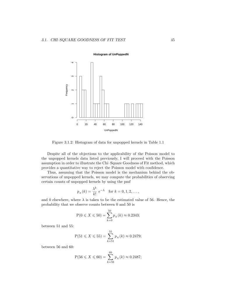
We begin with the example of determining whether the counts of unpoppedkernels in one–quarter cup shown in Table 1.1 on page 6 can be accounted forby a Poisson(�) distribution, where � is the average number of unpopped kernelsin one quarter cup. A point estimate for � is then given by the average of thevalues in the table; namely, 56. Before we proceed any further, I must point outthat the reason that I am assuming a Poisson model for the data in Table 1.1 ismerely for the sake of illustration of the Chi–Square test that we’ll be discussingin this section. However, a motivation for the use of the Poisson model is thata Poisson random variable is a limit of binomial random variables as n tends toinfinity under the condition that np = � remains constant (see your solution toProblem 5 in Assignment 2). However, this line of reasoning would be justifiedif the probability that a given kernel will not pop is small, which is not reallyjustified in this situation since, by the result in Example 2.2.2 on page 17, a 95%confidence interval for p is (0.109, 0.183). In addition, a look at the histogramof the data in Table 1.1, shown in Figure 3.1.2, reveals that the shape of thatdistribution for the number of unpopped kernels is far from being Poisson. Thereason for this is that the right tail of a Poisson distribution should be thinnerthan that of the distribution shown in Figure 3.1.2.

Moreover, calculation of the sample variance for the data in Table 1.1 yields1810, which is way too far from the sample mean of 56. Recall that the meanand variance of a Poisson(�) distribution are both equal to �.

3.1. CHI–SQUARE GOODNESS OF FIT TEST 45

Histogram of UnPoppedN

UnPoppedN

Fre

quen

cy

0 20 40 60 80 100 120 140

01

23

4

Figure 3.1.2: Histogram of data for unpopped kernels in Table 1.1

Despite all of the objections to the applicability of the Poisson model tothe unpopped kernels data listed previously, I will proceed with the Poissonassumption in order to illustrate the Chi–Square Goodness of Fit method, whichprovides a quantitative way to reject the Poisson model with confidence.

Thus, assuming that the Poisson model is the mechanism behind the ob-servations of unpopped kernels, we may compute the probabilities of observingcertain counts of unpopped kernels by using the pmf

pX

(k) =�k

k!e−� for k = 0, 1, 2, . . . ,

and 0 elsewhere, where � is taken to be the estimated value of 56. Hence, theprobability that we observe counts between 0 and 50 is

P(0 ⩽ X ⩽ 50) =

50∑k=0

pX

(k) ≈ 0.2343;

between 51 and 55:

P(51 ⩽ X ⩽ 55) =

55∑k=51

pX

(k) ≈ 0.2479;

between 56 and 60:

P(56 ⩽ X ⩽ 60) =

60∑k=56

pX

(k) ≈ 0.2487;


and 61 and above:

P(X ⩾ 61) =

∞∑k=61

pX

(k) ≈ 0.2691.

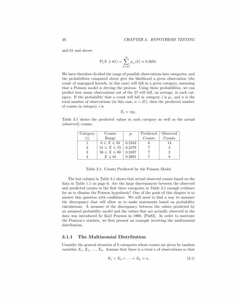
We have therefore divided the range of possible observations into categories, andthe probabilities computed above give the likelihood a given observation (thecount of unpopped kernels, in this case) will fall in a given category, assumingthat a Poisson model is driving the process. Using these probabilities, we canpredict how many observations out of the 27 will fall, on average, in each cat-egory. If the probability that a count will fall in category i is pi, and n is thetotal number of observations (in this case, n = 27), then the predicted numberof counts in category i is

Ei = npi.

Table 3.1 shows the predicted values in each category as well as the actual(observed) counts.

Category Counts pi Predicted Observed(i) Range Counts Counts1 0 ⩽ X ⩽ 50 0.2343 6 142 51 ⩽ X ⩽ 55 0.2479 7 33 56 ⩽ X ⩽ 60 0.2487 7 24 X ⩾ 61 0.2691 7 8

Table 3.1: Counts Predicted by the Poisson Model

The last column in Table 3.1 shows that actual observed counts based on thedata in Table 1.1 on page 6. Are the large discrepancies between the observedand predicted counts in the first three categories in Table 3.1 enough evidencefor us to dismiss the Poisson hypothesis? One of the goals of this chapter is toanswer this question with confidence. We will need to find a way to measurethe discrepancy that will allow us to make statements based on probabilitycalculations. A measure of the discrepancy between the values predicted byan assumed probability model and the values that are actually observed in thedata was introduced by Karl Pearson in 1900, [Pla83]. In order to motivatethe Pearson’s statistic, we first present an example involving the multinomialdistribution.

3.1.1 The Multinomial Distribution

Consider the general situation of k categories whose counts are given by randomvariables X1, X1, . . . , Xk. Assume that there is a total n of observations so that

X1 +X2 + ⋅ ⋅ ⋅+Xk = n. (3.1)


We assume that the probability that a count is going to fall in category i is pifor i = 1, 2, . . . , k. Assume also that the categories are mutually exclusive andexhaustive so that

p1 + p2 + ⋅ ⋅ ⋅+ pk = 1. (3.2)

Then, the distribution of the random vector

X = (X1, X2, . . . , Xk) (3.3)

is multinomial so that the joint pmf of the random variables X1, X1, . . . , Xk,given that X1 +X2 + ⋅ ⋅ ⋅+Xk = n, is

p(X1,X2,...,Xk)

(n1, n2, . . . , nk) =

⎧⎨⎩n!

n1!n2! ⋅ ⋅ ⋅nk!pn1

1 pn22 ⋅ ⋅ ⋅ p

nkk if

∑ki=1 nk = n;

0 otherwise.

(3.4)We first show that eachXi has marginal distribution which is binomial(n, pi),

so thatE(Xi) = npi for all i = 1, 2, . . . , k,

andvar((Xi)) = npi(1− pi) for all i = 1, 2, . . . , k.

Note that the X1, X2, . . . , Xk are not independent because of the relation in(3.1). In fact, it can be shown that

cov(Xi, Xj) = −npjpj for i ∕= j.

We will first establish that the marginal distribution of Xi is binomial. Wewill show it for X1 in the following example. The proof for the other variablesis similar. In the proof, though, we will need the following extension of thebinomial theorem known as the multinomial theorem [CB01, Theorem 4.6.4, p.181].

Theorem 3.1.1 (Multinomial Theorem). Let n, n1, n2, . . . , nk denote non–negative integers, and a1, a2, . . . , ak be real numbers. Then,

(a1 + a2 + ⋅ ⋅ ⋅+ ak)n =∑

n1+n2+⋅⋅⋅+nk=n

n!

n1!n2! ⋅ ⋅ ⋅nk!an1

1 an22 ⋅ ⋅ ⋅ a

nkk ,

where the sum is take over all k–tuples of nonnegative integers, n1, n2, . . . , nkwhich add up to n.

Remark 3.1.2. Note that when k = 2 in Theorem 3.1.1 we recover the binomialtheorem,

Example 3.1.3. Let (X1, X2, . . . , Xk) have a multinomil distribution with pa-rameters n, p1, p2, . . . , pk. Then, the marginal distribution ofX1 is binomial(n, p1).


Solution: The marginal distribution of X1 has pmf

pX1

(n1) =∑

n2,n3,...,nkn2+n3+...+nk=n−n1

n!

n1!n2! ⋅ ⋅ ⋅nk!pn1

1 pn22 ⋅ ⋅ ⋅ p

nkk ,

where the summation is taken over all nonnegative, integer values ofn2, n3, . . . , nk which add up to n− n1. We then have that

pX1

(n1) =pn1

1

n1!

∑n2,n3,...,nk

n2+n3+...+nk=n−n1

n!

n2! ⋅ ⋅ ⋅nk!pn2

2 ⋅ ⋅ ⋅ pnkk

=pn1

1

n1!

n!

(n− n1)!

∑n2,n3,...,nk

n2+n3+...+nk=n−n1

(n− n1)!

n2! ⋅ ⋅ ⋅nk!pn2

2 ⋅ ⋅ ⋅ pnkk

=

(n

n1

)pn1

1 (p2 + p3 + ⋅ ⋅ ⋅+ pk)n−n1 ,

where we have applied the multinomial theorem (Theorem 3.1.1).Using (3.2) we then obtain that

pX1

(n1) =

(n

n1

)pn1

1 (1− p1)n−n1 ,

which is the pmf of a binomial(n, p1) distribution. □

3.1.2 The Pearson Chi-Square Statistic

We first consider the example of a multinomial random vector (X1, X2) withparameters n, p1, p2; in other words, there are only two categories and the countsin each category are binomial(n, pi) for i = 1, 2, with X1 +X2 = n. We considerthe situation when n is very large. In this case, the random variable

Z =X1 − np1√np1(1− p1)

has an approximate normal(0, 1) distribution for large values of n. Consequently,for large values of n,

Z2 =(X1 − np1)2

np1(1− p1)

has an approximate �2(1) distribution.


Note that we can write

Z2 =(X1 − np1)2(1− p1) + (X1 − np1)2p1

np1(1− p1)

=(X1 − np1)2

np1+

(X1 − np1)2

n(1− p1)

=(X1 − np1)2

np1+

(n−X2 − np1)2

n(1− p1)

=(X1 − np1)2

np1+

(X2 − n(1− p1))2

n(1− p1)

=(X1 − np1)2

np1+

(X2 − np2)2

np2.

We have therefore proved that, for large values of n, the random variable

Q =(X1 − np1)2

np1+

(X2 − np2)2

np2

has an approximate �2(1) distribution.The random variable Q is the Pearson Chi–Square statistic for k = 2.

Theorem 3.1.4 (Pearson Chi–Square Statistic). Let (X1, X2, . . . , Xk) be a ran-dom vector with a multinomial(n, p1, . . . , pk) distribution. The random variable

Q =

k∑i=1

(Xi − npi)2

npi(3.5)

has an approximate �2(k − 1) distribution for large values of n. If the pisare computed assuming an underlying distribution with c unknown parameters,then the number of degrees of freedom in the chi–square distribution for Q getreduced by c. In other words

Q ∼ �2(k − c− 1) for large values of n.

Theorem 3.1.4, the proof of which is relegated to Appendix A on page 87 inthese notes, forms the basis for the Chi–Square Goodness of Fit Test. Examplesof the application of this result will be given in subsequent sections.

3.1.3 Goodness of Fit Test

We now go back to the analysis of the data portrayed in Table 3.1 on page 46.Letting X1, X2, X3, X4 denote the observed counts in the fourth column of the


table, we compute the value of the Pearson Chi–Square statistic according to(3.5) to be

Q =

4∑i=1

(Xi − npi)2

npi≈ 16.67,

where, in this case, n = 27 and the pis are given in the third column of Table3.1. This is the measure of how far the observed counts are from the countspredicted by the Poisson assumption. How significant is the number 16.67? Isit a big number or not? More importantly, how probable would a value like16.67, or higher, be if the Poisson assumption is true? The last question isone we could answer approximately by using Pearson’s Theorem 3.1.4. Since,Q ∼ �2(2) in this case, the answer to the last question is

p = P(Q > 16.67) ≈ 0.0002,

or 0.02%, less than 1%, which is a very small probability. Thus, the chances ofobserving the counts in the fourth column of Table 3.1 on page 46, under theassumption that the Poisson hypothesis is true, are very small. The fact thatwe did observe those counts, and the counts came from observations recorded inTable 1.1 on page 6 suggest that it is highly unlikely that the counts of unpoppedkernels in that table follow a Poisson distribution. We are therefore justified inrejecting the Poisson hypothesis on the basis on not enough statistical supportprovided by the data.

3.2 The Language and Logic of Hypothesis Tests

The argument that we followed in the example presented in the previous sectionis typical of hypothesis tests.

∙ Postulate a Null Hypothesis. First, we postulated a hypothesis thatpurports to explain patters observed in data. This hypothesis is the oneto be tested against the data. In the example at hand, we want to testwhether the counts of unpopped kernels in a one–quarter cup follow aPoisson distribution. The Poisson assumption was used to determineprobabilities that observations will fall into one of four categories. Wecan use these values to formulate a null hypothesis, Ho, in terms of thethe predicted probabilities; we write

Ho : p1 = 0.2343, p2 = 0.2479, p3 = 0.2487, p4 = 0.2691.

Based on probabilities in Ho, we compute the expected counts in eachcategories

Ei = npi for i = 1, 2, 3, 4.

Remark 3.2.1 (Why were the categories chosen the way we chose them?).Pearson’s Theorem 3.1.4 gives an approximate distribution for the Chi–Square statistic in (3.5) for large values of n. A rule of thumb to justify

3.2. THE LANGUAGE AND LOGIC OF HYPOTHESIS TESTS 51

the use the Chi–Square approximation to distribution of the Chi–Squarestatistic, Q, is to make sure that the expected count in each category is 5or more. That is why we divided the range of counts in Table 1.1 on page6 into the four categories shown in Table 3.1 on page 46.

∙ Compute a Test Statistic. In the example of the previous section,we computed the Pearson Chi–Square statistic, Q, which measures howfar the observed counts, X1, X2, X3, X4, are from the expected counts,E1, E2, E3, E4:

Q =

4∑i=1

(Xi − Ei)2

Ei.

According to Pearson’s Theorem, the random variable Q given by (3.5);namely,

Q =

4∑i=1

(Xi − npi)2

npi

has an approximate �2(4− 1− 1) distribution in this case.

∙ Compute or approximate a p–value. A p–value for a test is theprobability that the test statistic will attain the computed value, or moreextreme ones, under the assumption that the null hypothesis is true. Inthe example of the previous section, we used the fact that Q has an ap-proximate �2(2) distribution to compute

p–value = P(Q ⩾ Q).

∙ Make a decision. Either we reject or we don’t reject the null hypothesis.The criterion for rejection is some threshold, � with 0 < � < 1, usuallysome small probability, say � = 0.01 or � = 0.05.

We reject Ho if p–value < �; otherwise we don’t reject Ho.

We usually refer to � as a level of significance for the test. If p–value < �we say that we reject Ho at the level of significance �.

In the example of the previous section

p–value ≈ 0.0002 < 0.01;

Thus, we reject the Poisson model as an explanation of the distribution forthe counts of unpopped kernels in Table 1.1 on page 6 at the significancelevel of � = 1%.

Example 3.2.2 (Testing a binomial model). We have seen how to use a chi–square goodness of fit test to determine that the Poisson model for the distribu-tion of counts of unpopped kernels in Table 1.1 on page 6 is not supported bythe data in the table. A more appropriate model would be a binomial model.In this case we have two unknown parameters: the mean number of kernels,


n, in one–quarter cup, and the probability, p, that a given kernel will not pop.We have estimated n independently using the data in Table 1.2 on page 8 tobe n = 342 according to the result in Example 2.3.13 on page 42. In order toestimate p, we may use the average number of unppoped kernels in one–quartercup from the data in Table 1.1 on page 6 and then divide that number by theestimated value of n to obtain the estimate

p =56

342≈ 0.1637.

Thus, in this example, we assume that the counts, X, of unpopped kernels inone–quarter cup in Table 1.1 on page 6 follows the distribution

X ∼ binomial(n, p).

Category Counts pi Predicted Observed(i) Range Counts Counts1 0 ⩽ X ⩽ 50 0.2131 6 142 51 ⩽ X ⩽ 55 0.2652 7 33 56 ⩽ X ⩽ 60 0.2700 7 24 X ⩾ 61 0.2517 7 8

Table 3.2: Counts Predicted by the Binomial Model

Table 3.2 shows the probabilities predicted by the binomial hypothesis ineach of the categories that we used in the previous example in which we testedthe Poisson hypothesis. Observe that the binomial model predicts the sameexpected counts as the Poisson model. We therefore get the same value forthe Pearson Chi–Square statistic, Q = 16.67. In this case the approximate,asymptotic distribution of Q is �2(1) because we estimated two parameters, nand p, to compute the pis. Thus, the p–value in this case is approximated by

p–value ≈ 4.45× 10−5,

which is a very small probability. Thus, we reject the binomial hypothesis.Hence the hypothesis that distribution of the counts of unpopped kernels followsa binomial model is not supported by the data. Consequently, the intervalestimate for p which we obtained in Example 2.2.2 on page 17 is not justifiedsince that interval was obtained under the assumption of a binomial model. Wetherefore need to come up with another way to obtain an interval estimate forp.

At this point we need to re–evaluate the model and re–examine the assump-tions that went into the choice of the Poisson and binomial distributions aspossible explanations for the distribution of counts in Table 1.1 on page 6. Animportant assumption that goes into the derivations of both models is that of

3.2. THE LANGUAGE AND LOGIC OF HYPOTHESIS TESTS 53

independent trials. In this case, a trial consists of determining whether a givenkernel will pop or not. It was mentioned in Section 1.1.1 that a kernel in a hot–air popper might not pop because it gets pushed out of the container because ofthe popping of kernels in the neighborhood of the given kernel. Thus, the eventthat a kernel will not pop will depend on whether a nearby kernel popped ornot, and no necessarily on some intrinsic property of the kernel. These consid-erations are not consistent with the independence assumption required by boutthe Poisson and the binomial models. Thus, these models are not appropriatefor this situation.

How we proceed from this point on will depend on which question we wantto answer. If we want to know what the intrinsic probability of not poppingfor a given kernel is, independent of the popping mechanism that is used, weneed to redesign the experiment so that the popping procedure that is usedwill guarantee the independence of trials required by the binomial or Poissonmodels. For example, a given number of kernels, n, might be laid out on flatsurface in a microwave oven.

If we want to know what the probability of not popping is for the hot–air popper, we need to come up with another way to model the distribution.This process is complicated by the fact that there are two mechanisms at workthat prevent a given from popping: an intrinsic mechanism depending on theproperties of a given kernel, and the swirling about of the kernels in the containerthat makes it easy for the popping of a given kernel to cause other kernels tobe pushed out before they pop. Both of these mechanisms need to be modeled.

Example 3.2.3 (A test of normality). In this example we test whether thecounts of kernels in one–quarter cup shown in Table 1.2 on page 8 can beassumed to come from a normal distribution. We first use the data in the tableto estimate � and �2. Based on the calculations in Example 2.3.13 on page 42,we get the following estimates

� = Xn ≈ 342,

and

� = Sn ≈ 35.

We therefore assume that

N ∼ normal(�, �2)

and use the corresponding pdf to compute the probabilities that the counts willlie in certain ranges.

Table 3.3 on page 54 shows those ranges and their corresponding probabili-ties. Note that the ranges for the counts were chosen so that the expected countfor each category is 5. Table 3.3 shows also the predicted and observed countsfrom which we get the value for the chi–square statistic, Q, to be Q = 2/5.In this case Q has an approximate �2(1) asymptotic distribution, according to


Category Counts pi Predicted Observed(i) Range Counts Counts1 N ⩽ 319 0.2555 5 62 319 < N ⩽ 342 0.2445 5 53 342 < N ⩽ 365 0.2445 5 54 N > 365 0.2555 5 4

Table 3.3: Kernels in 1/4–cup Predicted by the Normal Model

Pearson’s Theorem, since we estimated two parameters, � and �, based on thedata. We therefore obtain the approximate p–value

p–value = P(Q ⩾ Q) ≈ 0.5271.

Thus, based on the data, we cannot reject the null hypothesis that the countscan be described as following a normal distribution. Hence, we were justifiedin assuming a normal model when estimating the mean number of kernels inone–quarter cup in Example 2.3.13 on page 42.

3.3 Hypothesis Tests in General

Hypothesis testing is a tool in statistical inference which provides a generalframework for rejecting certain hypothesis, known as the null hypothesis anddenoted by Ho, against an alternative hypothesis, denoted by H1. For in-stance, in Example 3.2.3 on page 53 we tested the hypothesis that the countsof kernel in a one–quarter cup, shown in Table 1.2 on page 8, follows a normaldistribution. In this case, denoting the counts of kernels by N , we may statethe null and alternative hypotheses as

Ho : N is normaly distributed

andH1 : N is not normaly distributed.

Here is another example.

Example 3.3.1. We wish to determine whether a given coin is fair or not.Thus, we test the null hypothesis

Ho : p =1

2

versus the alternative hypothesis

H1 : p ∕= 1

2,

where p denotes the probability that a given toss of the coin will yield a head.

3.3. HYPOTHESIS TESTS IN GENERAL 55

In order to tests the hypotheses in Example 3.3.1, we may perform an ex-periment which consists of flipping the coin 400 times. If we let Y denote thenumber of heads that we observe, then Ho may be stated as

Ho : Y ∼ binomial(400, 0.5).

Notice that this hypothesis completely specifies the distribution of the randomvariable Y , which is known as a test statistic. On the other hand, the hy-pothesis in the goodness of fit test in Example 3.2.3 on page 53 does not specifya distribution. Ho in Example 3.2.3 simply states that the the count, N , ofkernels in one–quarter cup follows a normal distribution, but it does not specifythe parameters � and �2.

Definition 3.3.2 (Simple versus Composite Hypotheses). A hypothesis whichcompletely specifies a distribution is said to be a simple hypothesis. A hy-pothesis which is not simple is said to be composite.

For example, the alternative hypothesis, H1 : p ∕= 0.5, in Example 3.3.1 iscomposite since the test statistic, Y , for that test is binomial(400, p) where p isany value between 0 and 1 which is not 0.5. Thus, H1 is a really a combinationof many hypotheses.

The decision to reject or not reject Ho in a hypothesis test is based on aset of observations, X1, X2, . . . , Xn; these could be the outcomes of certain ex-periment performed to test the hypothesis and are, therefore, random variableswith certain distribution. Given a set of of observations, X1, X2, . . . , Xn, a teststatistic, T = T (X1, X2, . . . , Xn), may be formed. For instance, in Example3.3.1 on page 54, the experiment might consist of flipping the coin 400 timesand determining the number of heads. If the null hypothesis in that test is true,then the 400 observations are independent Bernoulli(0.5) trials. We can definethe test statistic for this test to be

T =

400∑i=1

Xi

so that, in Ho is true,T ∼ binomial(400, 0.5).

A test statistic for a hypothesis test may be used to establish a criterion forrejecting Ho. For instance in the coin tossing Example 3.3.1, we can say thatwe reject the hypothesis that the coin is fair if

∣T − 200∣ > c; (3.6)

that is, the distance from the statistic T to the mean of the assumed distributionis at least certain critical value, c. The condition in (3.6) constitutes a decisioncriterion for rejection of Ho. It the null hypothesis is true and the observedvalue, T , of the test statistic, T , falls within the range specified by the rejectioncriterion in (3.6), we mistakenly reject Ho when it is in fact true. This is known


as a Type I error. The probability of committing a Type I error in the cointossing example is

P (∣T − 200∣ > c ∣ Ho true) .

Definition 3.3.3 (Significance Level). The largest probability of making a typeI error is denoted by � and is called the significance level of the test.

Example 3.3.4. In the coin tossing example (Example 3.3.1), we can set a givensignificance level, �, as follows. Since the number of tosses is large, n = 400, wecan use the central limit theorem to get that

P (∣T − 200∣ > c ∣ Ho true) = P

(∣T − 200∣√

400 ⋅ (0.5)(1− 0.5)>

c

10

)

≈ P(∣Z∣ > c

10

),

where Z ∼ normal(0, 1). It then follows that, if we set

c

10= z�/2,

where z�/2 is such that P(∣Z∣ > z�/2) = �, we obtain that c = 10z�/2. Hence,the rejection criterion

∣T − 200∣ > 10z�/2

yields a test with a significance level �. For example, if � = 0.05, then we getthat z�/2 = 1.96 and therefore c = 19.6 ≈ 20. Hence, the test that rejects Ho if

T < 180 or T > 220

has a significance level of � = 0.05.

If the null hypothesis, Ho, is in fact false, but the hypothesis test does notyield the rejection of Ho, then a type II error is made. The probability of a typeII error is denoted by �.

In general, a hypothesis test is concerned with the question of whether aparameter, �, from certain underlying distribution is in a certain range or not.Suppose the underlying distribution has pdf or pmf denoted by f(x ∣ �), wherewe have explicitly expressed the dependence of the distribution function on theparameter �; for instance, in Example 3.3.1, the underlying distribution is

f(x ∣ p) = px(1− p)1−x, for x = 0 or x = 1,

and 0 otherwise. The parameter � in this case is p, the probability of a successin a Bernoulli(p) trial.

In the general setting, the null and alternative hypothesis are statements ofthe form

Ho : � ∈ Ωo


andH1 : � ∈ Ω1

where Ωo and Ω1 are complementary subsets of a parameter space Ω = Ωo∪Ω1,where Ωo ∩ Ω1 = ∅. In Example 3.3.1, we have that Ωo = {0.5} and

Ω1 = {p ∈ [0, 1] ∣ p ∕= 0.5}.

Given a set of observations, X1, X2, . . . , Xn, which may be assumed to beiid random variables with distribution f(x ∣ �), we denote the set all possiblevalues of the n–tuple (X1, X2, . . . , Xn) by D. Consider a statistic

T = T (X1, X2, . . . , Xn).

A rejection region, R, for a test is defined by

R = {(x1, x2, . . . , xn) ∈ D ∣ T (x1, x2, . . . , xn) ∈ A}, (3.7)

where A is a subset of the real line. For example, in the coin tossing example,we had the rejection region

R = {(x1, x2, . . . , xn) ∈ D ∣ ∣T (x1, x2, . . . , xn)− E(T )∣ > c},

orR = {(x1, x2, . . . , xn) ∈ D ∣ ∣T (x1, x2, . . . , xn)− np∣ > c},

since, this this case, T ∼ binomial(n, p), where n = 400, and p depends onwhich hypothesis we are assuming to be true. Thus, in this case, the set A inthe definition of the rejection region in (3.7) is

A = (−∞, np− c) ∪ (np+ c,∞).

Given a rejection region, R, for a test of hypotheses

Ho : � ∈ Ωo

andH1 : � ∈ Ω1,

letP�((x1, x1, . . . , xn) ∈ R)

denote the probability that the observation values fall in the rejection regionunder the assumption that the random variables X1, X2, . . . , Xn are iid withdistribution f(x ∣ �). Thus,

max�∈Ωo

P�((x1, x1, . . . , xn) ∈ R)

is the largest probability that Ho will be rejected given that Ho; this is thesignificance level for the test; that is,

� = max�∈Ωo

P�((x1, x1, . . . , xn) ∈ R).


In Example 3.3.1 on page 54, Ωo = {0.5}; thus,

� = P0.5 ((x1, x2, . . . , xn) ∈ R) ,

where

R = {(x1, x2, . . . , xn) ∣ T (x1, x2, . . . , xn) < np−c, or T (x1, x2, . . . , xn) > np+c}.

By the same token, for � ∈ Ω1,

P�((x1, x1, . . . , xn) ∈ R)

gives the probability of rejecting the null hypothesis when Ho is false. It thenfollows that the probability of a Type II error, for the case in which � ∈ Ω1, is

�(�) = 1− P�((x1, x1, . . . , xn) ∈ R);

this is the probability of not rejecting the null hypothesis when Ho is in factfalse.

Definition 3.3.5 (Power of a Test). For � ∈ Ω1, the function

P� ((x1, x1, . . . , xn) ∈ R))

is called the power function for the test at �; that is, P� ((x1, x1, . . . , xn) ∈ R))is the probability of rejecting the null hypothesis when it is in fact false. Wewill use the notation

(�) = P� ((x1, x1, . . . , xn) ∈ R)) for � ∈ Ω1.

Example 3.3.6. In Example 3.3.1 on page 54, consider the rejection region

R = {(x1, x2, . . . , xn) ∈ D ∣ ∣T (x1, x2, . . . , xn)− 200∣ > 20}

where

T (x1, x2, . . . , xn) =

n∑j=1

xj ,

for n = 400, in the test of Ho : p = 0.5 against H1 : p ∕= 0.5. The significancelevel for this test is

� = P0.5 (∣T − 200∣ > 20) ,

whereT ∼ binomial(400, 0.5).

Thus,� = 1− P (∣T − 200∣ ⩽ 20)

= 1− P (180 ⩽ T ⩽ 220)

= 1− P (179.5 < T ⩽ 220.5) ,


where we have used the continuity correction, since we are going to be applyingthe Central Limit Theorem to approximate a discrete distribution; namely, Thas an approximate normal(200, 100) distribution in this case, since n = 400 islarge. We then have that

� ≈ 1− P (179.5 < Y ⩽ 220.5) ,

where Y ∼ normal(200, 100). Consequently,

� ≈ 1− (FY

(220.5)− FY

(179.5)),

where FY

is cdf of Y ∼ normal(200, 100). We then have that

� ≈ 0.0404.

We next compute the power function for this test:

(p) = P(∣T − 200∣ > 20),

where

T ∼ binomial(400, p) for p ∕= 1

2.

We write (p) = P(∣T − 200∣ > 20)

= 1− P(∣T − 200∣ ⩽ 20)

= 1− P(180 ⩽ T ⩽ 220)

= 1− P(179.5 < T ⩽ 220.5),

where we have used again the continuity correction, since we are going to beapplying the Central Limit Theorem to approximate the distribution of T bythat of a normal(400p, 400p(1− p)) random variable. We then have that

(p) ≈ 1− P(179.5 < Yp ⩽ 220.5),

where Yp denotes a normal(400p, 400p(1− p)) random variable. Thus,

(p) ≈ 1− (FYp

(220.5)− FYp

(179.5)), (3.8)

where FYp

denotes the cdf of Yp ∼ normal(400p, 400p(1− p)).Table 3.4 on page 60 shows a few values of p and their corresponding ap-

proximate values of (p) according to (3.8). A sketch of the graph of as afunction of p is shown in Figure 3.3.3 on page 61.

The sketch in Figure 3.3.3 was obtained using the plot function in R bytyping

plot(p,gammap,type=’l’,ylab="Power at p")


p (p)0.10 1.00000.20 1.00000.30 1.00000.40 0.97670.43 0.77560.44 0.63780.45 0.48000.46 0.32600.47 0.19780.48 0.10760.49 0.05660.50 0.04040.51 0.05660.52 0.10760.53 0.19780.54 0.32600.55 0.48000.56 0.63780.57 0.77560.60 0.97670.70 1.00000.80 1.00000.90 1.0000

Table 3.4: Table of values of p and (p)

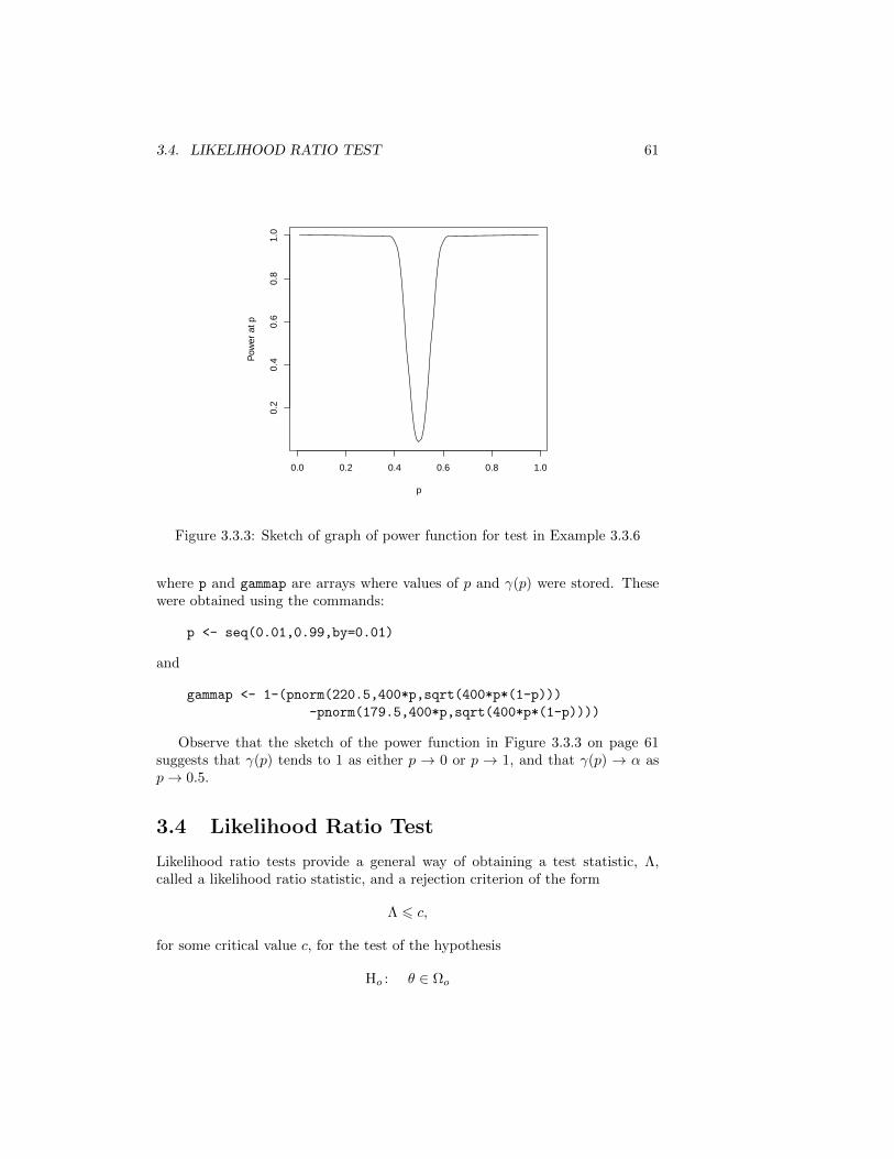
3.4. LIKELIHOOD RATIO TEST 61

0.0 0.2 0.4 0.6 0.8 1.0

0.2

0.4

0.6

0.8

1.0

p

Pow

er a

t p

Figure 3.3.3: Sketch of graph of power function for test in Example 3.3.6

where p and gammap are arrays where values of p and (p) were stored. Thesewere obtained using the commands:

p <- seq(0.01,0.99,by=0.01)

and

gammap <- 1-(pnorm(220.5,400*p,sqrt(400*p*(1-p)))

-pnorm(179.5,400*p,sqrt(400*p*(1-p))))

Observe that the sketch of the power function in Figure 3.3.3 on page 61suggests that (p) tends to 1 as either p → 0 or p → 1, and that (p) → � asp→ 0.5.

3.4 Likelihood Ratio Test

Likelihood ratio tests provide a general way of obtaining a test statistic, Λ,called a likelihood ratio statistic, and a rejection criterion of the form

Λ ⩽ c,

for some critical value c, for the test of the hypothesis

Ho : � ∈ Ωo


versus the alternativeH1 : � ∈ Ω1,

based on a random sample, X1, X2, . . . , Xn, coming a distribution with distri-bution function f(x ∣ �). Here f(x ∣ �) represents a pdf or a pmf, Ω = Ωo ∪ Ω1

is the parameter space, and Ωo ∩ Ω1 = ∅.Before we define the likelihood ratio statistic, Λ, we need to define the con-

cept of a likelihood function.

Definition 3.4.1 (Likelihood Function). Given a random sample, X1, X2, . . . , Xn,from a distribution with distribution function f(x ∣ �), either a pdf or a pmf,where � is some unknown parameter (either a scalar or a vector parameter), thejoint distribution of the sample is given by

f(x1, x2, . . . , xn ∣ �) = f(x1 ∣ �) ⋅ f(x2 ∣ �) ⋅ ⋅ ⋅ f(xn ∣ �),

by the independence condition in the definition of a random sample. If therandom variables, X1, X2, . . . , Xn, are discrete, f(x1, x2, . . . , xn ∣ �) gives theprobability of observing the values

X1 = x1, X2 = x2, . . . , Xn = xn,

under the assumption that the sample is taken from certain distribution withparameter �. We can also interpret f(x1, x2, . . . , xn ∣ �o) as measuring thelikelihood that the parameter � will take on the value �o given that we haveobserved the values x1, x2, . . . , xn in the sample. Thus, we call

f(x1, x2, . . . , xn ∣ �)

the likelihood function for the parameter � given the observations

X1 = x1, X2 = x2, . . . , Xn = xn,

and denote it by L(� ∣ x1, x2, . . . , xn); that is,

L(� ∣ x1, x2, . . . , xn) = f(x1, x2, . . . , xn ∣ �).

Example 3.4.2 (Likelihood function for independent Bernoulli(p) trials). LetX1, X2, . . . , Xn be a random sample from a Bernoulli(p). Thus, the underlyingdistribution in this case is

f(x ∣ p) = px(1− p)1−x for x = 0, 1 and 0 otherwise,

where 0 < p < 1.We then get that the likelihood function for p, based on the sample obser-

vations, is

L(p ∣ x1, x2, . . . , xn) = px1(1− p)1−x1 ⋅ px2(1− p)1−x2 ⋅ ⋅ ⋅ pxn(1− p)1−xn

= py(1− p)n−y

where y =

n∑i=1

xi.


Definition 3.4.3 (Likelihood Ratio Statistic). For a general hypothesis test of

Ho : � ∈ Ωo

against the alternative

H1 : � ∈ Ω1,

based on a random sample, X1, X2, . . . , Xn, from a distribution with distributionfunction f(x ∣ �), the likelihood ratio statistic, Λ(x1, x2, . . . , xn), is definedby

Λ(x1, x2, . . . , xn) =

sup�∈Ωo

L(� ∣ x1, x2, . . . , xn)

sup�∈Ω

L(� ∣ x1, x2, . . . , xn),

where Ω = Ωo ∪ Ω1 with Ωo ∩ Ω1 = ∅.

Example 3.4.4 (Simple hypotheses for Bernoulli(p) trials). Consider the testof

Ho : p = po

versus

H1 : p = p1,

where p1 ∕= po, based on random sample of size n from a Bernoulli(p) distribu-tion, for 0 < p < 1. The likelihood ratio statistic for this test is

Λ(x1, x2, . . . , xn) =L(po ∣ x1, x2, . . . , xn)

max{L(po ∣ x1, x2, . . . , xn), L(p1 ∣ x1, x2, . . . , xn)},

since, for this case, Ωo = {po} and Ω = {po, p1}; thus,

Λ(x1, x2, . . . , xn) =pyo(1− po)n−y

max{pyo(1− po)n−y, py1(1− p1)n−y},

where y =n∑i=1

xi.

Definition 3.4.5 (Likelihood Ratio Test). We can use the likelihood ratiostatistic, Λ(x1, x2, . . . , xn), to define the rejection region

R = {(x1, x2, . . . , xn) ∣ Λ(x1, x2, . . . , xn) ⩽ c},

for some critical value c with 0 < c < 1. This defines a likelihood ratio test(LRT) for Ho against H1.

The rationale for this definition is that, if the likelihood ratio of the sampleis very small, the evidence provided by the sample in favor of the null hypothesisis not strong in comparison with the evidence for the alternative. Thus, in thiscase it makes sense to reject Ho.


Example 3.4.6. Find the likelihood ratio test for

Ho : p = po

versus

H1 : p = p1,

for po ∕= p1, based on a random sample X1, X2, . . . , Xn from a Bernoulli(p)distribution for 0 < p < 1.

Solution: The rejection region for the likelihood ratio test is givenby

R : Λ(x1, x2, . . . , xn) ⩽ c,

for 0 < c < 1, where

Λ(x1, x2, . . . , xn) =pyo(1− po)n−y

max{pyo(1− po)n−y, py1(1− p1)n−y},

with

y =

n∑i=1

xi.

Thus, for R to be defined, we must have that

Λ(x1, x2, . . . , xn) =pyo(1− po)n−y

py1(1− p1)n−y;

otherwise Λ(x1, x2, . . . , xn) would be 1, and so we wouldn’t be ableto get the condition Λ(x1, x2, . . . , xn) ⩽ c to hold since c < 1. Thus,the LRT for this example will reject Ho if(

pop1

)y (1− po1− p1

)n−y⩽ c,

or (1− po1− p1

)n(po(1− p1)

p1(1− po)

)y⩽ c.

Write

a =1− po1− p1

and r =po(1− p1)

p1(1− po).

Then, the LRT rejection region is defined by

anry ⩽ c, (3.9)

where

y =

n∑i=1

xi.


We consider two cases:

Case 1: p1 > po. In this case, a > 1 and r < 1. Thus, taking thenatural logarithm on both sides of (3.9) and solving for y we get thatthe rejection region for the LRT in this example is equivalent to

y ⩾ln c− n ln a

ln r.

In other words, the LRT will reject Ho if

Y ⩾ b,

where b =ln (c/an)

ln r> 0, and Y is the statistic

Y =

n∑i=1

Xi,

which counts the number of successes in the sample.

Case 2: p1 < po. In this case, a < 1 and r > 1. We then get from(3.9) the LRT in this example rejects Ho if

y ⩽ln c− n ln a

ln r.

In other words, the LRT will reject Ho if

Y ⩽ d,

where d =ln c− n ln a

ln rcan be made to be positive by choosing

n >ln c

ln a, and Y is again the number of successes in the sample. □

We next consider the example in which we test

Ho : p = po

versus

H1 : p ∕= p0

based on a random sample X1, X2, . . . , Xn from a Bernoulli(p) distribution for0 < p < 1. We would like to find the LRT rejection region for this test ofhypotheses.

In this case the likelihood ratio statistic is

Λ(x1, x2, . . . , xn) =L(po ∣ x1, x2, . . . , xn)

sup1<p<1

L(p ∣ x1, x2, . . . , xn), (3.10)


where L(p ∣ x1, x2, . . . , xn) = py(1− p)n−y for y =

n∑i=1

xi.

In order to determine the denominator in the likelihood ratio in (3.10), weneed to maximize the function L(p ∣ x1, x2, . . . , xn) over 0 < p < 1. We can dothis by maximizing the natural logarithm of the likelihood function,

ℓ(p) = ln(L(p ∣ x1, x2, . . . , xn)), 0 < p < 1,

since ln : (0,∞)→ ℝ is a strictly increasing function. Thus, we need to maximize

ℓ(p) = y ln p+ (n− y) ln(1− p) over 0 < p < 1.

In order to do this, we compute the derivatives

ℓ′(p) =y

p− n− y

1− p,

and

ℓ′′(p) = − y

p2− n− y

(1− p)2,

and observe that ℓ′′(p) < 0 for all 1 < p < 1. Thus, a critical point of ℓ; that is,a solution of ℓ′(p) = 0, will yield a maximum for the function ℓ(p).

Solving for p in ℓ′(p) = 0 yields the critical point

p =1

ny,

which is the sample proportion of successes. This is an example of a maximumlikelihood estimator (MLE) for p. In general, we have the following definition.

Definition 3.4.7 (Maximum Likelihood Estimator). Let X1, X2, . . . , Xn be arandom sample from a distribution with distribution function f(x ∣ �), for � in

some parameter space Ω. A value, �, of the parameter � such that

L(� ∣ x1, x2, . . . , xn) = sup�∈Ω

L(� ∣ x1, x2, . . . , xn)

is called a maximum likelihood estimator for �, or an MLE for �.

We therefore have that the likelihood ratio statistic for the test of Ho : p = poversus H1 : p ∕= po, based on a random sample of size n from a Bernoulli(p)distribution, is

Λ(x1, x2, . . . , xn) =pyo(1− po)n−y

py(1− p)n−y,

where

y =

n∑i=1

xi

and

p =1

ny


is the MLE for p based on the random sample.Write the likelihood ratio statistic as

Λ(x1, x2, . . . , xn) =

(pop

)y (1− po1− p

)n−y

=

(pop

)y⎛⎜⎜⎝1

po− 1

1

po− p

po

⎞⎟⎟⎠n−y

,

and set t =p

po. Then, Λ can be written as a function of t as follows

Λ(t) =1

tnpot⋅(

1− po1− pot

)n−npot, for 0 ⩽ t ⩽

1

po,

where we have used the fact that p =1

ny so that y = npot.

We now proceed to sketch the graph of Λ as a function of t for 0 ⩽ t ⩽1

po.

First note that Λ(t) attains its maximum value of 1 when t = 1; namely,when p = po. That t = 1 is the only value of t at which the maximum for Λ(t)is attained can be verified by showing that

ℎ(t) = ln(Λ(t)) = −npot ln t− (n− npot) ln

(1− pot1− po

)attains its maximum solely at t = 1. Computing the derivative of ℎ with respectto t we find that

ℎ′(t) = −npo ln t+ npo ln

(1− pot1− po

)

= npo ln

(1− pott(1− po)

).

Thus, ℎ′(t) = 0 if and only if

1− pott(1− po)

= 1,

which implies that t = 1 is the only critical point of ℎ. The fact that t = 1yields a maximum for ℎ can be seen by observing that the second derivative ofℎ with respect to t,

ℎ′′(t) = −npot− np2

o

1− pot,

is negative for 0 < t <1

po.


Observe also that limt→0+

ℎ(t) = ln[(1 − po)n] and limt→(1/po)−

ℎ(t) = ln[pno ], so

that

Λ(0) = (1− po)n and Λ(1/po) = pno .

Putting all the information about the graph for Λ(t) together we obtain a sketchas the one shown in Figure 3.4.4,where we have sketched the case po = 1/4 andn = 20 for 0 ⩽ t ⩽ 4. The sketch in Figure 3.4.4 suggests that, given any

0 1 2 3 4

0.0

0.2

0.4

0.6

0.8

1.0

t

Lmab

da(t

)

Figure 3.4.4: Sketch of graph of Λ(t) for po = 1/4, n = 20, and 0 ⩽ t ⩽ 4

positive value of c such that c < 1 and c > max{pno , (1 − po)n}, there exist

positive values t1 and t2 such that 0 < t1 < 1 < t2 < 1/po and

Λ(t) = c for t = t1, t2.

Furthermore,

Λ(t) ⩽ c for t ⩽ t1 or t ⩾ t2.

Thus, the LRT rejection region for the test of Ho : p = po versus H1 : p ∕= po isequivalent to

p

po⩽ t1 or

p

po⩾ t2,

which we could rephrase in terms of Y =

n∑i=1

Xi as

R : Y ⩽ t1npo or Y ⩾ t2npo,


for some t1 and t2 with 0 < t1 < 1 < t2. This rejection region can also bephrased as

R : Y < npo − b or Y > npo + b,

for some b > 0. The value of b will then be determined by the significance levelthat we want to impose on the test.

Example 3.4.8 (Likelihood ratio test based on a sample from a normal distri-bution). We wish to test the hypothesis

Ho : � = �o, �2 > 0

versus the alternativeH1 : � ∕= �o, �

2 > 0,

based on a random sample, X1, X2, . . . , Xn, from a normal(�, �2) distribution.Observe that both Ho and H1 are composite hypotheses.

The likelihood function in this case is

L(�, � ∣ x1, x2, . . . , xn) =e−(x1−�)2/2�2

√2� �

⋅ e−(x2−�)2/2�2

√2� �

⋅ ⋅ ⋅ e−(xn−�)2/2�2

√2� �

=e−∑ni=1(xi−�)2/2�2

(2�)n/2 �n.

The likelihood ratio statistic is

Λ(x1, x2, . . . , xn) =

sup�>0

L(�o, � ∣ x1, x2, . . . , xn)

L(�, � ∣ x1, x2, . . . , xn), (3.11)

where � is the MLE for � and �2 is the MLE for �2. To find these MLEs, weneed to maximize the natural logarithm of the likelihood function:

ℓ(�, � ∣ x1, x2, . . . , xn) = − 1

2�2

n∑i=1

(xi − �)2 − n ln� − n

2ln(2�).

We therefore need to look at the first partial derivatives

∂ℓ

∂�(�, �) =

1

�2

n∑i=1

(xi − �) =n

�2(x− �)

∂ℓ

∂�(�, �) =

1

�3

n∑i=1

(xi − �)2 − n

�,

where x =1

n

n∑i=1

xi, and the second partial derivatives

∂2ℓ

∂�2(�, �) = − n

�2,


∂2ℓ

∂�∂�(�, �) =

∂2ℓ

∂�∂�(�, �) = −2n

�3(x− �),

and∂2ℓ

∂�2(�, �) = − 3

�4

n∑i=1

(xi − �)2 +n

�2,

The critical points of ℓ(�, �) are solutions to the system⎧⎨⎩∂ℓ

∂�(�, �) = 0

∂ℓ

∂�(�, �) = 0,

which yields� = x,

�2 =1

n

n∑i=1

(xi − x)2.

To see that ℓ(�, �) is maximized at these values, look at the Hessian matrix,⎛⎜⎜⎜⎜⎝∂2ℓ

∂�2(�, �)

∂2ℓ

∂�∂�(�, �)

∂2ℓ

∂�∂�(�, �)

∂2ℓ

∂�2(�, �)

⎞⎟⎟⎟⎟⎠ ,

at (�, �) to get ⎛⎜⎜⎝− n

�20

0 −2n

�2

⎞⎟⎟⎠ ,

which has negative eigenvalues. It then follows that ℓ(�, �) is maximized at(�, �). Hence, x is the MLE for � and

�2 =1

n

n∑i=1

(xi − x)2

is the MLE for �2. Observe that �2 is not the sample variance, S2n. In fact,

�2 =n− 1

nS2n,

so that

E(�2) =n− 1

n�2,


and so �2 is not an unbiased estimator of �2. It is, however, the maximumlikelihood estimator of �2.

We then have that the denominator in the likelihood ratio in (3.11) is

L(�, � ∣ x1, x2, . . . , xn) =e−∑ni=1(xi−x)2/2�2

(2�)n/2 �n=

e−n/2

(2�)n/2 �n.

To compute the numerator in (3.11), we need to maximize

ℓ(�) = ln(L(�o, � ∣ x1, x2, . . . , xn))

= − 1

2�2

n∑i=1

(xi − �o)2 − n ln� − n

2ln(2�).

Taking derivatives of ℓ we obtain

ℓ′(�) =1

�3

n∑i=1

(xi − �o)2 − n

�

and

ℓ′′(�) = − 3

�4

n∑i=1

(xi − �o)2 +n

�2.

Thus, a critical point of ℓ(�) is the value, �, of � given by

�2 =1

n

n∑i=1

(xi − �o)2.

Note that

ℓ′′(�) = −2n

�2 < 0,

so that ℓ(�) is maximized when � = �. We then have that

sup�>0

L(�o, � ∣ x1, x2, . . . xn) = L(�o, � ∣ x1, x2, . . . xn),

where

�2 =1

n

n∑i=1

(xi − �o)2.

Observe that

n∑i=1

(xi − �o)2 =

n∑i=1

(xi − x+ x− �o)2

=

n∑i=1

(xi − x)2 +

n∑i=1

(x− �o)2,


sincen∑i=1

2(xi − x)(x− �o) = 2(x− �o)n∑i=1

(xi − x) = 0.

We then have that�2 = �2 + (x− �o)2. (3.12)

Consequently,

sup�>0

L(�o, � ∣ x1, x2, . . . xn) =e−∑ni=1(xi−�o)2/2�2

(2�)n/2 �n=

e−n/2

(2�)n/2 �n.

Thus, the likelihood ratio statistic in (3.11) is

Λ(x1, x2, . . . , xn) =

sup�>0

L(�o, � ∣ x1, x2, . . . , xn)

L(�, � ∣ x1, x2, . . . , xn)=�n

�n.

Hence, an LRT will reject Ho is

�n

�n⩽ c,

for some c with 0 < c < 1, or�2

�2 ⩽ c2/n,

or�2

�2⩾

1

c2/n,

where1

c2/n> 1. In view of (3.12), we see that and LRT will reject Ho if

(x− �o)2

�2⩾

1

c2/n− 1 ≡ k,

where k > 0, and �2 is the MLE for �2. Writingn− 1

nS2n for �2 we see that

an LRT will reject Ho if

∣x− �o∣Sn/√n⩾√

(n− 1)k ≡ b,

where b > 0. Hence, the LRT can be based in the test statistic

Tn =Xn − �oSn/√n.

Note that Tn has a t(n−1) distribution if Ho is true. We then see that if t�/2,n−1

is such thatP(∣T ∣ ⩾ t�/2,n−1) = �, for T ∼ t(n− 1),

3.5. THE NEYMAN–PEARSON LEMMA 73

then the LRT of Ho : � = �o versus H1 : � ∕= �o which rejects Ho if

∣Xn − �o∣Sn/√n⩾ t�/2,n−1,

has significance level �.Observe also that the set of values of �o which do not get rejected by this

test is the open interval(Xn − t�/2,n−1

Sn√n,Xn + t�/2,n−1

Sn√n

),

which is a 100(1− �)% confidence interval for the mean, �, of a normal(�, �2)distribution based on a random sample of size n from that distribution. Thisprovides another interpretation of a confidence interval based on a hypothesistest.

3.5 The Neyman–Pearson Lemma

Consider a test of a simple hypothesis

Ho : � = �o

versus the alternativeH1 : � = �1

based on a random sample of size n from a distribution with distribution func-tion f(x ∣ �). The likelihood ratio statistic in this case is

Λ(x1, x2, . . . , xn) =L(�o ∣ x1, x2, . . . , xn)

L(�1 ∣ x1, x2, . . . , xn). (3.13)

The rejection region for the LRT is

R = {(x1, x2, . . . , xn) ∣ Λ(x1, x2, . . . , xn) ⩽ c} (3.14)

for some 0 < c < 1.If the significance level of the test is �, then

� =

∫R

f(x1, x2, . . . , xn ∣ �o) dx1dx2 ⋅ ⋅ ⋅ dxn,

for the case in which f(x ∣ �) is a pdf. Thus,

� =

∫R

L(�o ∣ x1, x2, . . . , xn) dx1dx2 ⋅ ⋅ ⋅ dxn, (3.15)

It then follows that the power of the LRT is

(�1) =

∫R

L(�1 ∣ x1, x2, . . . , xn) dx1dx2 ⋅ ⋅ ⋅ dxn; (3.16)


that is, the probability of reject Ho when H1 is true.Consider next another test with rejection region R and significance level �.

We then have that

� =

∫R

L(�o ∣ x1, x2, . . . , xn) dx1dx2 ⋅ ⋅ ⋅ dxn, (3.17)

and the power of the new test is

(�1) =

∫R

L(�1 ∣ x1, x2, . . . , xn) dx1dx2 ⋅ ⋅ ⋅ dxn. (3.18)

The Neyman–Pearson Lemma states that

(�1) ⩽ (�1); (3.19)

in other words, out of all the tests of the simple hypothesis Ho : � = �o versusH1 : � = �1, the LRT yields the largest possible power. Consequently, theLRT gives the smallest probability of making a Type II error our of the tests ofsignificance level �.

The proof of the Neyman–Pearson Lemma is straight forward. First observethat

R = (R ∩ R) ∪ (R ∩ Rc), (3.20)

where Rc denotes the complement of R. It then follows from (3.15) that

� =

∫R∩R

L(�o ∣ x) dx +

∫R∩Rc

L(�o ∣ x) dx, (3.21)

where we have abbreviated the vector (x1, x2, . . . , xn) by x, and the volumeelement dx1dx2 ⋅ ⋅ ⋅ dxn by dx. Similarly, using

R = (R ∩R) ∪ (R ∩Rc), (3.22)

and (3.17) we get that

� =

∫R∩R

L(�o ∣ x) dx +

∫R∩Rc

L(�o ∣ x) dx. (3.23)

Combining (3.21) and (3.23) we then get that∫R∩Rc

L(�o ∣ x) dx =

∫R∩Rc

L(�o ∣ x) dx. (3.24)

To prove (3.19), use (3.18) and (3.22) to get

(�1) =

∫R∩R

L(�1 ∣ x) dx +

∫R∩Rc

L(�1 ∣ x) dx (3.25)

Similarly, using (3.16) and (3.20), we get that

(�1) =

∫R∩R

L(�1 ∣ x) dx +

∫R∩Rc

L(�1 ∣ x) dx. (3.26)

3.5. THE NEYMAN–PEARSON LEMMA 75

Next, subtract (3.25) from (3.26) to get

(�1)− (�1) =

∫R∩Rc

L(�1 ∣ x) dx−∫R∩Rc

L(�1 ∣ x) dx, (3.27)

and observe thatcL(�1 ∣ x) ⩾ L(�o ∣ x) on R ∩ Rc (3.28)

andcL(�1 ∣ x) ⩽ L(�o ∣ x) on R ∩Rc, (3.29)

where we have used (3.13) and (3.14). Multiplying the inequality in (3.29) by−1 we get that

−cL(�1 ∣ x) ⩾ −L(�o ∣ x) on R ∩Rc. (3.30)

It then follows from (3.27), (3.28) and (3.30)

(�1)− (�1) ⩾1

c

(∫R∩Rc

L(�o ∣ x) dx−∫R∩Rc

L(�o ∣ x) dx

)= 0 (3.31)

where we have used (3.24). The inequality in (3.19) now follows from (3.31).Thus, we have proved the Neymann–Pearson Lemma.

The Neyman–Pearson Lemma applies only to tests of simple hypotheses.For instance, in Example 3.4.6 of page 64 dealing with the test of Ho : p = poversus H1 : p = p1, for p1 > po, based on a random sample X1, X2, . . . , Xn froma Bernoulli(p) distribution for 0 < p < 1, we saw that the LRT rejects the nullhypothesis at some significance level, �, is

Y =

n∑i=1

Xi ⩾ b, (3.32)

for some b > 0 determined by �. By the Neyman–Pearson Lemma, this is themost powerful test at that significance level; that is, the test with the smallestprobability of a Type II error. Recall that the value of b yielding a significancelevel � may be obtained, for large sample sizes, n, by applying the Central LimitTheorem. In fact, assuming that the null hypothesis is true, the test statistic Yin (3.32) is binomial(n, po). We then have that

� = P(Y ⩾ b)

= P

(Y − npo√npo(1− po)

⩾b− npo√npo(1− po)

)

≈ P

(Z ⩾

b− npo√npo(1− po)

),

where Z ∼ normal(0, 1). Thus, if z� is such that P(Z ⩾ z�) = �, then

b = npo + z�√npo(1− po) (3.33)


in (3.32) gives the most powerful test at the significance level of �. Observethat this value of b depends only on po and n; it does not depend on p1.

Now consider the test of Ho : p = po versus H1 : p > po. Since, the alterna-tive hypothesis is not simple, we cannot apply the Neyman–Pearson Lemma di-rectly. However, by the previous considerations, the test that rejects Ho : p = poif

Y ⩾ b,

where b is given by (3.33) for large n is the most powerful test at level � for everyp1 > po; i.e., for every possible value in the alternative hypothesis H1 : p > po.We then say that the LRT is the uniformly most powerful test (UMP) atlevel � in this case.

Definition 3.5.1 (Uniformly most powerful test). A test of a simple hypothesisHo : � = �o against a composite alternative hypothesis H1 : � ∈ Ω1 is said tobe uniformly most powerful test (UMP) at a level �, if it is most powerfulat that level for every simple alternative � = �1 in Ω1.

Chapter 4

Evaluating Estimators

Given a random sample, X1, X2, . . . , Xn, from a distribution with distributionfunction f(x ∣ �), we have seen that there might be more than one statistic,

T = T (X1, X2, . . . , Xn),

that can be used to estimate the parameter �. For example, if X1, X2, . . . , Xn isa random sample from a normal(�, �2) distribution, then the sample variance,

S2n =

1

n− 1

n∑i=1

(Xi −Xn)2,

and the maximum likelihood estimator,

�2 =1

n

n∑i=1

(Xi −Xn)2,

are both estimators for the variance �2. The sample variance, S2n, is unbiased,

while the MLE is not.As another example, consider a random sample, X1, X2, . . . , Xn, from a

Poisson distribution with parameter �. Then, the sample mean, Xn and thethen the sample variance, S2

n. are both unbiased estimators for �.Given two estimators for a given parameter, �, is there a way to evaluate

the two estimators in such a way that we can tell which of the two is the betterone? In this chapter we explore one way to measure how good an estimator is,the mean squared error or MSE. We will then see how to use that measure tocompare one estimator to others.

4.1 Mean Squared Error

Given a random sample, X1, X2, . . . , Xn, from a distribution with distributionfunction f(x ∣ �), and an estimator, W = W (X1, X2, . . . , Xn), for the parameter

77

78 CHAPTER 4. EVALUATING ESTIMATORS

�, we define the mean squared error (MSE) of W to be the expected valueof (W − �)2. We denote this expected value by E

�

[(W − �)2

]and compute it,

for the case in which f(x ∣ �) is a pdf, using the formula

E�

[(W − �)2

]=

∫ℝn

(W − �)2f(x1, x2, . . . , xn ∣ �) dx1dx2 ⋅ ⋅ ⋅ dxn,

where f(x1, x2, . . . , xn ∣ �) is the joint distribution of the sample. The subscript,�, in the expectation symbol for expectation, E, reminds us that we are usingf(x1, x2, . . . , xn ∣ �). By the same token, the expectation of the W is writtenE�(W ). We also write

MSE(W ) = E�

[(W − �)2

].

Observe that, since expectation is a linear operation,

MSE(W ) = E�

[((W − E

�(W )) + (E

�(W )− �))2

]= E

�

[((W − E

�(W )))2 + 2(W − E

�(W ))(E

�(W )− �) + (E

�(W )− �)2

]= E

�

[(W − E

�(W ))2

]+ E

�

[(E

�(W )− �)2

]since

E�

[2(W − E�(W ))(E

�(W )− �)] = 2(E

�(W )− �) E

�[(W − E

�(W )]

= 2(E�(W )− �) [E

�(W )− E

�(W )]

= 0.

We then have that

MSE(W ) = var�(W ) + [E

�(W )− �]2;

that is, the mean square error of W is the sum of the variance of W and thequantity [E

�(W ) − �]2. The expression E

�(W ) − � is called the bias of the

estimator W and is denoted by bias�(W ); that is,

bias�(W ) = E

�(W )− �.

We then have that the mean square error of an estimator is

MSE(W ) = var�(W ) + [bias

�(W )]2.

Thus, if the estimator, W , is unbiased, then E�(W ) = �, so that

MSE(W ) = var�(W ), for an unbiased estimator.

4.1. MEAN SQUARED ERROR 79

Example 4.1.1. Let X1, X2, . . . , Xn be a random sample from a normal(�, �2)distribution. Then, the sample mean, Xn, and the sample variance, S2

n, areunbiased estimators of the � and �2, respectively. It then follows that

MSE(Xn) = var(Xn) =�2

n

and

MSE(S2n) = var(S2

n) =2�4

n− 1,

where we have used the fact that

n− 1

�2S2n ∼ �2(n− 1),

and therefore(n− 1)2

�4var(S2

n) = 2(n− 1).

Example 4.1.2 (Comparing the sample variance and the MLE in a samplefrom a norma distribution). Let X1, X2, . . . , Xn be a random sample from anormal(�, �2) distribution. The MLE for �2 is the estimator

�2 =1

n

n∑i=1

(Xi −Xn)2.

Since �2 =n− 1

nS2n, and S2

n is an unbiased estimator for � it follows that

E(�2) =n− 1

n�2 = �2 − �2

n.

It then follows that the bias of �2 is

bias(�2) = E(�2)− �2 = −�2

n,

which shows that, on average, �2 underestimates �2.Next, we compute the variance of �2. In order to do this, we used the fact

thatn− 1

�2S2n ∼ �2(n− 1),

so that

var

(n− 1

�2S2n

)= 2(n− 1).

It then follows from �2 =n− 1

nS2n that

n2

�4var(�2) = 2(n− 1),


so that

var(�2) =2(n− 1)�4

n2.

It the follows that the mean squared error of �2 is

MSE(�2) = var(�2) + bias(�2)

=2(n− 1)�4

n2+�4

n2

=2n− 1

n2�4.

Comparing the value of MSE(�2) to

MSE(S2n) =

2�4

n− 1,

we see thatMSE(�2) < MSE(S2

n).

Hence, the MLE for �2 has a smaller mean squared error than the unbiasedestimator S2

n. Thus, �2 is a more precise estimator than S2n; however, S2

n ismore accurate than �2.

4.2 Cramer–Rao Theorem

If W = W (X1, X2, . . . , Xn) is an unbiased estimator for �, where X1, X2, . . . , Xn

is a random sample from a distribution with distribution function f(x ∣ �), wesaw in the previous section that the mean squared error of W is given by

MSE(W ) = var�(W ).

The question we would like to answer in this section is the following: Out of allunbiased estimators of � based on the random sample X1, X2, . . . , Xn, is thereone with the smallest possible variance, and consequently the smallest possibleMSE?

We will provide a partial answer to the question posed above. The answeris based on a lower bound for the variance of a statistic, W , based on a randomsample from a distribution with distribution function f(x ∣ �). The lower boundwas discovered independently by Rao and Cramer around the middle of thetwentieth century. The idea is to show that

var�(W ) ⩾ b(�, n)

for all estimators, W , based on the sample, for a function b of the parameter�. The Cramer–Rao inequality can be derived as a consequence of the Cauchy–Schwarz inequality: For any statistics, W1 and W2, based on the sample,

[cov(W1,W2)]2 ⩽ var(W1) ⋅ var(W2). (4.1)

4.2. CRAMER–RAO THEOREM 81

The proof of (4.1) is very straightforward. Define a function ℎ : ℝ→ ℝ by

ℎ(t) = var(W1 + tW2) for all t ∈ ℝ,

and observe that ℎ(t) ⩾ 0 for all t ∈ ℝ. By the properties of the expectationoperator and the definition of variance,

ℎ(t) = E[(W1 + tW2)2

]− [E(W1 + tW2)]

2

= E[W 2

1 + 2tW1W2 + t2W 22

]− [E(W1) + tE(W2)]

2

= E[W 2

1

]+ 2tE [W1W2] + t2E

[W 2

2

]− [E(W1)]

2 − 2tE(W1)E(W2)− t2 [E(W2)]2

= var(W1) + 2 cov(W1,W2) t+ var(W2) t2,

where we have used the definition of covariance

cov(W1,W2) = E(W1W2)− E(W1)E(W2). (4.2)

It then follows that ℎ(t) is quadratic polynomial which is never negative. Con-sequently, the discriminant,

[2 cov(W1,W2)]2 − 4 var(W2)var(W1),

is at most 0; that is,

4 [cov(W1,W2)]2 − 4 var(W2)var(W1) ⩽ 0,

from which the Cauchy–Schwarz inequality in (4.1) follows.To obtain the Crammer–Rao lower bound, we will apply the Cauchy–Schwarz

inequality (4.1) to the case W1 = W and

W2 =∂

∂�[ln (L(� ∣ X1, X2, . . . , Xn))] .

In other words, W1 is the estimator in question and W2 is the partial deriva-tive with respect to the parameter � of the natural logarithm of the likelihoodfunction.

In order to compute cov(W1,W2), we will need the expected value of W2.Note that

W2 =1

L(� ∣ X1, X2, . . . Xn)

∂

∂�[L(� ∣ X1, X2, . . . , Xn)] ,

so that

E�(W2) =

∫ℝn

1

L(� ∣ x)

∂

∂�[L(� ∣ x)] L(� ∣ x) dx,

where we have denoted the vector (x1, x2, . . . , xn) by x and the volume element,dx1dx2 ⋅ ⋅ ⋅ dxn, by dx. We then have that

E�(W2) =

∫ℝn

∂

∂�[L(� ∣ x)] dx.


Assuming that the order of differentiation and integration can be changed, wethen have that

E�(W2) =

∂

∂�

[∫ℝnL(� ∣ (x)) dx

]=

∂

∂�(1) = 0,

so that W2 has expected value 0. It then follows from (4.2) that

cov(W1,W2) = E�(W1W2)

=

∫ℝnW (x)

1

L(� ∣ x)

∂

∂�[L(� ∣ x)] L(� ∣ x) dx

=

∫ℝnW (x)

∂

∂�[L(� ∣ x)] dx

=

∫ℝn

∂

∂�[W (x) L(� ∣ x)] dx.

Thus, if the order of differentiation and integration can be interchanged, wehave that

cov(W1,W2) =∂

∂�

[∫ℝnW (x) L(� ∣ x) dx

]

=∂

∂�[E

�(W )] .

Thus, if we setg(�) = E

�(W )

for all � in the parameter range, we see that

cov�(W1,W2) = g′(�).

In particular, if W is an unbiased estimator, cov�(W,W2) = 1, where

W2 =∂

∂�[ln (L(� ∣ X1, X2, . . . , Xn))] .

Applying the Cauchy–Schwarz inequality in (4.1) we then have that

[g′(�)]2 ⩽ var(W ) ⋅ var(W2). (4.3)

In order to compute var(W2), observe that

W2 =∂

∂�

(n∑i=1

ln(f(Xi ∣ �)

)

=

n∑i=1

∂

∂�(ln(f(Xi ∣ �)) .


Thus, since X1, X2, . . . , Xn are iid random variable with distribution functionf(x ∣ �),

var(W2) =

n∑i=1

var

(∂

∂�(ln(f(Xi ∣ �))

)

= n ⋅ var

(∂

∂�(ln(f(Xi ∣ �))

)The variance of the random variable

∂

∂�[ln (f(X ∣ �))] is called the Fisher

Information and is denoted by I(�). We then have that

var(W2) = nI(�).

We then obtain from (4.3) that

[g′(�)]2 ⩽ nI(�) var(W ),

which yields the Cramer-Rao lower bound

var(W ) ⩾[g′(�)]2

nI(�), (4.4)

where

I(�) = var

(∂

∂�[ln (f(X ∣ �))]

)is the Fisher information. For the case in which W is unbiased we obtain from(4.4) that

var(W ) ⩾1

nI(�). (4.5)

Example 4.2.1. Let X1, X2, . . . , Xn be a random sample from a Poisson(�)distribution. Then,

f(X,�) =�X

X!e−�,

so thatln(f(X,�)) = X ln�− �− ln(X!)

and∂

∂�[ln(f(X,�))] =

X

�− 1.

Then the Fisher information is

I(�) =1

�2var(X) =

1

�2⋅ � =

1

�.

Thus, the Cramer–Rao lower bound for unbiased estimators is obtained from(4.5) to be

1

nI(�)=�

n.


Observe that if W = Xn, the sample mean, then W is unbiased and

var(W ) =�

n.

Thus, in this case, the lower bound for the variance of unbiased estimators isattained at the sample mean. We say that Xn is an efficient estimator.

Definition 4.2.2 (Efficient Estimator). An unbiased estimator, W , of a pa-rameter, �, is said to be efficient if its variance is the lower bound in theCramer–Rao inequality; that is, if

var(W ) =1

nI(�),

where I(�) is the Fisher information,

I(�) = var

(∂

∂�(ln(f(X ∣ �))

).

For any unbiased estimator, W , of �, we define the efficiency of W , denotedeff

�(W ), to be

eff�(W ) =

1/(nI(�))

var�(W )

.

Thus, by the Cramer–Rao inequality (4.5),

eff�(W ) ⩽ 1

for all unbiased estimators, W , of �. Furthermore, eff�(W ) = 1 if and only if W

is efficient.

Next, we turn to the question of computing the Fisher information, I(�).First, observe that

I(�) = var

(∂

∂�(ln(f(X ∣ �))

)= E

�

[(∂

∂�(ln(f(X ∣ �))

)2], (4.6)

since

E�

[∂

∂�(ln(f(X ∣ �))

]= 0. (4.7)

To see why (4.7) is true, observe that

E�

[∂

∂�(ln(f(X ∣ �))

]=

∫ ∞−∞

∂

∂�(ln(f(x ∣ �)) f(x ∣ �) dx

=

∫ ∞−∞

1

f(x ∣ �)∂

∂�(f(x ∣ �)) f(x ∣ �) dx

=

∫ ∞−∞

∂

∂�(f(x ∣ �)) dx

=∂

∂�

(∫ ∞−∞

f(x ∣ �) dx

),


assuming that the order of differentiation and integration can be interchanged.The identity in (4.7) now follows from the fact that∫ ∞

−∞f(x ∣ �) dx = 1.

Next, differentiate (4.7) with respect to � one more time to obtain that

∂

∂�E�

[∂

∂�(ln(f(X ∣ �))

]= 0, (4.8)

where, assuming that the order of differentiation and integration can be inter-changed,

∂

∂�E�

[∂

∂�(ln(f(x ∣ �))

]=

∂

∂�

[∫ ∞−∞

∂

∂�(ln(f(x ∣ �)) f(x ∣ �) dx

]

=

∫ ∞−∞

∂2

∂�2(ln(f(x ∣ �)) f(x ∣ �) dx

+

∫ ∞−∞

∂

∂�(ln(f(x ∣ �)) ∂

∂�f(x ∣ �) dx

= E�

[∂2

∂�2(ln(f(x ∣ �)))

]

+

∫ ∞−∞

1

f(x ∣ �)

[∂

∂�f(x ∣ �)

]2

dx,

where∫ ∞−∞

1

f(x ∣ �)

[∂

∂�f(x ∣ �)

]2

dx =

∫ ∞−∞

[1

f(x ∣ �)∂

∂�f(x ∣ �)

]2

f(x ∣ �) dx

=

∫ ∞−∞

[∂

∂�ln(f(x ∣ �))

]2

f(x ∣ �) dx

= E�

[(∂

∂�ln(f(x ∣ �))

)2].

It then follows from (4.6) that∫ ∞−∞

1

f(x ∣ �)

[∂

∂�f(x ∣ �)

]2

dx = I(�).

Consequently,

∂

∂�E�

[∂

∂�(ln(f(x ∣ �))

]= E

�

[∂2

∂�2(ln(f(x ∣ �)))

]+ I(�)


In view of (4.7) we therefore have that

I(�) = −E�

[∂2

∂�2(ln(f(x ∣ �)))

], (4.9)

which gives another formula for computing the Fisher information.

Appendix A

Pearson Chi–SquareStatistic

The goal of this appendix is to prove the first part of Theorem 3.1.4 on page49; namely: assume that

(X1, X2, . . . , Xk)

is a random vector with a multinomial(n, p1, p2, . . . , pk) distribution, and define

Q =

k∑i=1

(Xi − npi)2

npi. (A.1)

Then, for large values of n, Q has an approximate �2(k − 1) distribution. Theidea for the proof presented here comes from Exercise 3 on page 60 in [Fer02].

We saw is Section 3.1.2 that the result in Theorem 3.1.4 is true for k = 2.We begin the discussion in this appendix with the case k = 3. It is hoped thatthe main features of the proof of the general case will be seen in this simplecase.

Consider the random vector U = (U1, U2, U3) with a multinomial(1, p1, p2, p3)distribution. In other words, each component function, Ui, is a Bernoulli(pi)random variable for i = 1, 2, 3, and the distribution of U is conditioned on

U1 + U2 + U3 = 1.

We then have thatE(Uj) = pj for j = 1, 2, 3;

var(Uj) = pj(1− pj) for j = 1, 2, 3;

andcov(Ui, Uj) = −pipj for i ∕= j.

Suppose now that we have a sequence of independent multinomial(1, p1, p2, p3)random vectors

U1,U2, . . . ,Un, . . .

87

88 APPENDIX A. PEARSON CHI–SQUARE STATISTIC

We then have that the random vector

Xn = (X1, X2, X3) =

n∑i=1

Ui

has a multinomial(n, p1, p2, p3) distribution.We now try to get an expression for the Pearson chi–square statistic in (A.1),

for k = 3, in terms of the bivariate random vector

Wn =

(X1

X2

).

The expected value of the random vector Wn is

E(Wn) =

(np1

np2

),

and its covariance matrix is

CWn= n

(p1(1− p1) −p1p2

−p1p2 p2(1− p2)

),

or

CW = nC(U1,U2),

where C(U1,U2) is the covariance matrix for the bivariate random vector

(U1

U2

),

for (U1, U2, U3) ∼ multinomial(1, p1, p2, p3). Note that the determinant of thematrix C(U1,U2) is p1p2p3, which is different from 0 since we are assuming that

0 < pi < 1 for i = 1, 2, 3.

It then follows that C(U1,U2) is invertible with inverse

C−1(U1,U2) =

⎛⎜⎜⎜⎝1

p1+

1

p3

1

p3

1

p3

1

p2+

1

p3

⎞⎟⎟⎟⎠ .

Consequently,

n C−1Wn

=

⎛⎜⎜⎜⎝1

p1+

1

p3

1

p3

1

p3

1

p2+

1

p3

⎞⎟⎟⎟⎠ .

Note also that

(Wn − E(Wn))TC−1Wn

(Wn − E(Wn)),

89

where (Wn −E(Wn))T is the transpose of the column vector (Wn −E(Wn)),is equal to

n−1(X1 − np1, X2 − np2)

⎛⎜⎜⎜⎝1

p1+

1

p3

1

p3

1

p3

1

p2+

1

p3

⎞⎟⎟⎟⎠ .

⎛⎝X1 − np1

X2 − np2

⎞⎠ ,

which is equal to

n−1

(1

p1+

1

p3

)(X1 − np1)2

+n−1

p3(X1 − np1)(X2 − np2) +

n−1

p3(X2 − np2)(X1 − np1)

n−1

(1

p2+

1

p3

)(X2 − np2)2.

Note that

(X1 − np1)(X2 − np2) = (X1 − np1)(n−X1 −X3 − np2)

= (X1 − np1)(n(1− p2)−X1 −X3)

= (X1 − np1)(n(p1 + p3)−X1 −X3)

= −(X1 − np1)(X1 − np1 +X3 − np3)

= −(X1 − np1)2 − (X1 − np1)(X3 − np3).

Similarly, we obtain that

(X2 − np2)(X1 − np1) = −(X2 − np2)2 − (X2 − np2)(X3 − np3).

We then have that


(Wn − E(Wn))

is equal to

n−1

(1

p1+

1

p3− 1

p3

)(X1 − np1)2

−n−1

p3(X1 − np1)(X3 − np3)− n−1

p3(X2 − np2)(X3 − np3)

n−1

(1

p2+

1

p3− 1

p3

)(X2 − np2)2,


or1

np1(X1 − np1)2

− 1

np3(X3 − np3)[(X1 − np1) + (X2 − np2)]

1

np2(X2 − np2)2,

where

(X3 − np3)[(X1 − np1) + (X2 − np2)] = (X3 − np3)[X1 +X2 − n(p1 + p2)]

= (X3 − np3)[n−X3 − n(1− p3)]

= −(X3 − np3)2.

We have therefore shown that


(Wn − E(Wn))

is equal to

1

np1(X1 − np1)2 +

1

np3(X3 − np3)2 +

1

np2(X2 − np2)2;

that is,


(Wn − E(Wn)) =

3∑j=1

(Xj − npj)2

npj,

which is the Pearson Chi–Square statistic for the case k = 3. Consequently,

Q = (Wn − E(Wn))TC−1Wn

(Wn − E(Wn)).

Our goal now is to show that, as n→∞,


(Wn − E(Wn))

tends in distribution to a �2(2) random variable.Observe that the matrix C−1

Wnis symmetric and positive definite. There-

fore, it has a square root, C−1/2Wn

, which is also symmetric and positive definite.Consequently,

Q = (Wn − E(Wn))T(C−1/2Wn

)TC−1/2Wn

(Wn − E(Wn)),


Q = (C−1/2Wn

(Wn − E(Wn)))TC−1/2Wn

(Wn − E(Wn)).

91

Next, put

Zn = C−1/2Wn

(Wn − E(Wn))

and apply the multivariate central limit theorem (see, for instance, [Fer02, The-orem 5, p. 26]) to obtain that

ZnD−→ Z ∼ normal(0, I) as n→∞;

that is, the bivariate random vectors, Zn = C−1/2Wn

(Wn −E(Wn)), converge in

distribution to the bivariate random vector Z with mean

(00

)and covariance

matrix

I =

(1 00 1

).

In other words

Z =

(Z1

Z2

),

where Z1 and Z2 are independent normal(0, 1) random variables. Consequently,

(C−1/2Wn

(Wn − E(Wn))TC−1/2Wn

(Wn − E(Wn))D−→ ZTZ = Z2

1 + Z22

as n→∞; that is,

Q =

3∑i=1

(Xi − npi)2

npi

converges in distribution to a �2(2) random variable as n→∞, which we wantedto prove.

The proof of the general case is analogous. Begin with the multivariaterandom vector

(X1, X2, . . . , Xk) ∼ multinomial(n, p1, p2, . . . , pk).

Define the random vector

Wn =

⎛⎜⎜⎜⎝X1

X2

...Xk−1

⎞⎟⎟⎟⎠with covariance matrix CWn

. Verify that

Q =

k∑j=1

(Xj − npj)2

npj= (C

−1/2Wn

(Wn − E(Wn)))TC−1/2Wn

(Wn − E(Wn)).

Next, put

Zn = C−1/2Wn

(Wn − E(Wn))


and apply the multivariate central limit theorem to obtain that

ZnD−→ Z ∼ normal(0, I) as n→∞,

where I is the (k − 1)× (k − 1) identity matrix, so that

Z =

⎛⎜⎜⎜⎝Z1

Z2

...Zk−1

⎞⎟⎟⎟⎠ ,

where Z1, Z2, . . . , Zk−1 are independent normal(0, 1) random variables. Conse-quently,

(C−1/2Wn

(Wn − E(Wn))TC−1/2Wn

(Wn − E(Wn))D−→ ZTZ =

k−1∑j=1

Z2j ∼ �2(k − 1)

as n→∞. This proves that

Q =

k∑i=1

(Xi − npi)2

npi

converges in distribution to a �2(k − 1) random variable as n→∞.

Appendix B

The Variance of the SampleVariance

The main goal of this appendix is to compute the variance of the sample variancebased on a sample from and arbitrary distribution; i.e.,

var(S2n),

where

S2n =

1

n− 1

n∑i=1

(Xi −Xn)2.

We will come up with a formula based on the second and fourth centralmoments of the underlying distribution. More precisely, we will prove that

var(S2n) =

1

n

(�4 −

n− 3

n− 1�2

2

), (B.1)

where �2 denotes the second central moment, or variance, of the distributionand �4 is the fourth central moment.

In general, we define the first central moment, �1, of the distribution of Xto be

�1 = E(X),

the mean on the distribution. The second central moment of X, �2, is

�2 = E[(X − E(X))2

];

in other words, �2 is the variance of the distribution. Similarly, for any k ⩾ 2,the kth central moment, �k, of X is

�k = E[(X − E(X))k

].

93

94 APPENDIX B. THE VARIANCE OF THE SAMPLE VARIANCE

First observe that, for each i and j

(Xi −Xj)2 = (Xi −Xn +Xn −Xj)

2

= (Xi −Xn)2 − 2(Xi −Xn)(Xn −Xj) + (Xn −Xj)2,

so that∑i

∑j

(Xi −Xj)2 =

∑i

∑j

(Xi −Xn)2 +∑i

∑j

(Xj −Xn)2, (B.2)

since ∑i

∑j

(Xi −Xn)(Xn −Xj) =∑i

(Xi −Xn)∑j

(Xn −Xj) = 0.

It then follows from (B.2) that∑i

∑j

(Xi −Xj)2 = n

∑i

(Xi −Xn)2 + n∑j

(Xj −Xn)2

= n(n− 1)S2n + n(n− 1)S2

n

from which we obtain another formula for the sample variance:

S2n =

1

2n(n− 1)

∑i

∑j

(Xi −Xj)2,

which we can also write as

S2n =

1

n(n− 1)

∑∑i<j

(Xi −Xj)2. (B.3)

In order to compute var(S2n) we will need to compute the expectation of

(S2n)2, where, according to the formula in (B.3),

(S2n)2 =

1

n2(n− 1)2

∑∑i<j

∑∑k<ℓ

(Xi −Xj)2(Xk −Xℓ)

2.

It then follows by the linearity of the expectation operator that

E[(S2n)2]

=1

n2(n− 1)2

∑∑i<j

∑∑k<ℓ

E[(Xi −Xj)

2(Xk −Xℓ)2]. (B.4)

We will then to compute the expectations E[(Xi −Xj)

2(Xk −Xℓ)2]

for allpossible values of i, j, k, ℓ ranging from 1 to n such that i < j and k < ℓ. There

are

[n(n− 1)

2

]2

of those terms contributing to the expectation of (S2n)2 in

(B.4). Out of those terms,n(n− 1)

2, or

(n

2

), are of the form

E[(Xi −Xj)

4], (B.5)

95

where i < j. We compute the expectations in (B.5) as follows

E[(Xi −Xj)

4]

= E[(Xi − �1 + �1 −Xj)

4]

= E[(Xi − �1)4 + 4(Xi − �1)3(�1 −Xj)+6(Xi − �1)2(�1 −Xj)

2

+4(Xi − �1)(�1 −Xj)3 + (�1 −Xj)

4]

= �4 + 6�2 ⋅ �2 + �4,

where we have used the independence of the Xis and the definition of the centralmoments. We then have that

E[(Xi −Xj)

4]

= 2�4 + 6�22, for i ∕= j. (B.6)

For the rest for the expectations, E[(Xi −Xj)

2(Xk −Xℓ)2], in (B.4) there are

two possibilities

(i) i ∕= k and j ∕= ℓ, or

(ii) either i = k, or j = ℓ, but not both simultaneously.

In case (i) we obtain, by the independence of the Xis and the definition ofthe central moments, that

E[(Xi −Xj)

2(Xk −Xℓ)2]

= E[(Xi −Xj)

2]⋅ E[(Xk −Xℓ)

2], (B.7)

whereE[(Xi −Xj)

2]

= E[(Xi − �1 + �1 −Xj)

2]

= E[(Xi − �1)2

]+ E

[(Xj − �1)2

]since

E [(Xi − �1)(�1 −Xj)] = E(Xi − �1) ⋅ E(�1 −Xj) = 0.

Consequently,E[(Xi −Xj)

2]

= 2�2.

Similarly,E[(Xk −Xℓ)

2]

= 2�2.

We then have from (B.7) that

E[(Xi −Xj)

2(Xk −Xℓ)2]

= 4�22, for i ∕= j ∕= k ∕= ℓ. (B.8)

There are

4!

(n

4

)of making the choices for i ∕= j ∕= k ∕= ℓ. Since we are only interested in thosechoices with i < j and k < ℓ we get a total of

6

(n

4

)


choices in case (i). Consequently the number of choices in case (ii) is(n

2

)2

−(n

2

)− 6

(n

4

).

One of the expectations in case (ii) is of the form

E[(Xi −Xj)

2(Xi −Xℓ)2],

where j ∕= ℓ. In this case we have

E[(Xi −Xj)

2(Xi −Xℓ)2]

= E[(Xi − �1 + �1 −Xj)

2(Xi − �1 + �1 −Xℓ)2]

= E[(

(Xi − �1)2 + 2(Xi − �1)(�1 −Xj) + (�1 −Xj)2)(

(Xi − �1)2 + 2(Xi − �1)(�1 −Xℓ) + (�1 −Xℓ)2)]

= E[(Xi − �1)4 + 2(Xi − �1)3(�1 −Xℓ)+(Xi − �1)2(Xℓ − �1)2 + 2(Xi − �1)3(�1 −Xj)

+4(Xi − �1)2(�1 −Xj)(�1 −Xℓ)+2(Xi − �1)(�1 −Xj)(Xℓ − �1)2

+(Xi − �1)2(Xj − �1)2

+2(Xi − �1)(Xj − �1)2(�1 −Xℓ)+(Xj − �1)2(Xℓ − �1)2

].

Next, use the linearity of the expectation operator, the independence of Xi, Xj

and Xℓ, and the definition of the central moments to get

E[(Xi −Xj)

2(Xi −Xℓ)2]

= �4 + �2 ⋅ �2 + �2 ⋅ �2 + �2 ⋅ �2

= �4 + 3�22.

We obtain the same value for all the other expectations in case (ii); i.e.,

E[(Xi −Xj)

2(Xi −Xℓ)2]

= �4 + 3�22, for i ∕= j ∕= ℓ. (B.9)

It follows from (B.4) and the values of the possible expectations, E[(Xi −Xj)

2(Xk −Xℓ)2],

we have computed in equations (B.6), (B.8) and (B.9), that

E[n2(n− 1)2(S2

n)2]

=∑∑i<j

∑∑k<ℓ

E[(Xi −Xj)

2(Xk −Xℓ)2]

=

(n

2

)(2�4 + 6�2

2) + 6

(n

4

)(4�2

2)

+

((n

2

)2

−(n

2

)− 6

(n

4

))(�4 + 3�2

2).

Noting that

(n

2

)=n(n− 1)

2, the above expression simplifies to

E[n2(n− 1)2(S2

n)2]

= n(n− 1)(�4 + 3�22) + n(n− 1)(n− 2)(n− 3)�2

2

+n(n− 1)(n− 2)(�4 + 3�22).

97

Thus, dividing by n(n−1) on both sides of the previous equation we then obtainthat

E[n(n− 1)(S2

n)2]

= �4 + 3�22 + (n− 2)(n− 3)�2

2 + (n− 2)(�4 + 3�22)

= (n− 1)�4 + (n2 − 2n+ 3)�22.

Dividing by n− 1 we then have that

nE[(S2n)2]

= �4 +n2 − 2n+ 3

n− 1�2

2,

from which we obtain that

E[(S2n)2]

=1

n

(�4 +

n2 − 2n+ 3

n− 1�2

2

).

Thus,

var(S2n) = E

[(S2n)2]−[E(S2

n)]2

=1

n

(�4 +

n2 − 2n+ 3

n− 1�2

2

)− (�2)2,

since S2n is an unbiased estimator of �2. Simplifying we then obtain that

var(S2n) =

1

n�4 +

3− nn(n− 1)

�22,

which yields the equation in (B.1).

Bibliography

[CB01] G. Casella and R. L. Berger. Statistical Inference. Duxbury Press,second edition, 2001.

[Fer02] T. S. Ferguson. A Course in Large Sample Theory. Chapman &Hall/CRC, 2002.

[HCM04] R. V. Hogg, A. Craig, and J. W. McKean. Introduction to Mathemat-ical Statistics. Prentice Hall, 2004.

[Pla83] R. L. Plackett. Karl pearson and the chi–square test. InternationalStatistical Review, 51(1):59–72, April 1983.

[Stu08] Student. The probable error of a mean. Biometrika, 6(1):1–25, March1908.

99

statistical theory - pomona...

Documents