statistical signal processing of complex-valued data.pdf
TRANSCRIPT

8/21/2019 Statistical Signal Processing of Complex-Valued Data.pdf
http://slidepdf.com/reader/full/statistical-signal-processing-of-complex-valued-datapdf 1/330

8/21/2019 Statistical Signal Processing of Complex-Valued Data.pdf
http://slidepdf.com/reader/full/statistical-signal-processing-of-complex-valued-datapdf 2/330
This page intentionally left blank
8/21/2019 Statistical Signal Processing of Complex-Valued Data.pdf
http://slidepdf.com/reader/full/statistical-signal-processing-of-complex-valued-datapdf 3/330
Statistical Signal Processing of Complex-Valued Data
Complex-valued random signals are embedded into the very fabric of science and
engineering, yet the usual assumptions made about their statistical behavior are often
a poor representation of the underlying physics. This book deals with improper and noncircular complex signals, which do not conform to classical assumptions, and it
demonstrates how correct treatment of these signals can have significant payoffs.
The book begins with detailed coverage of the fundamental theory and presents a
variety of tools and algorithms for dealing with improper and noncircular signals. It pro-
vides a comprehensive account of the main applications, covering detection, estimation,
and signal analysis of stationary, nonstationary, and cyclostationary processes.
Providing a systematic development from the origin of complex signals to their
probabilistic description makes the theory accessible to newcomers. This book is ideal
for graduate students and researchers working with complex data in a range of researchareas from communications to oceanography.
PETER J. SCHREIER is an Associate Professor in the School of Electrical Engineering and
Computer Science, The University of Newcastle, Australia. He received his Ph.D. in
electrical engineering from the University of Colorado at Boulder in 2003. He currently
serves on the Editorial Board of the IEEE Transactions on Signal Processing , and on
the IEEE Technical Committee Machine Learning for Signal Processing .
LOUIS L. SCHARF is Professor of Electrical and Computer Engineering and Statistics at
Colorado State University. He received his Ph.D. from the University of Washington
at Seattle. He has since received numerous awards for his research contributions to
statistical signal processing, including an IEEE Distinguished Lectureship, an IEEE
Third Millennium Medal, and the Technical Achievement and Society Awards from the
IEEE Signal Processing Society. He is a Life Fellow of the IEEE.

8/21/2019 Statistical Signal Processing of Complex-Valued Data.pdf
http://slidepdf.com/reader/full/statistical-signal-processing-of-complex-valued-datapdf 4/330
8/21/2019 Statistical Signal Processing of Complex-Valued Data.pdf
http://slidepdf.com/reader/full/statistical-signal-processing-of-complex-valued-datapdf 5/330
Statistical Signal Processing
of Complex-Valued DataThe Theory of Improper and
Noncircular Signals
P E T E R J . S C H R E I E R
University of Newcastle, New South Wales, Australia
L O U I S L . S C H A R F
Colorado State University, Colorado, USA

8/21/2019 Statistical Signal Processing of Complex-Valued Data.pdf
http://slidepdf.com/reader/full/statistical-signal-processing-of-complex-valued-datapdf 6/330
CAMBRIDGE UNIVERSITY PRESS
Cambridge, New York, Melbourne, Madrid, Cape Town, Singapore,São Paulo, Delhi, Dubai, Tokyo
Cambridge University Press
The Edinburgh Building, Cambridge CB2 8RU, UK
First published in print format
ISBN-13 978-0-521-89772-3
ISBN-13 978-0-511-67772-4
© Cambridge University Press 2010
2010
Information on this title: www.cambridge.org/9780521897723
This publication is in copyright. Subject to statutory exception and to the
provision of relevant collective licensing agreements, no reproduction of any part
may take place without the written permission of Cambridge University Press.
Cambridge University Press has no responsibility for the persistence or accuracy
of urls for external or third-party internet websites referred to in this publication,
and does not guarantee that any content on such websites is, or will remain,
accurate or appropriate.
Published in the United States of America by Cambridge University Press, New York
www.cambridge.org
eBook (NetLibrary)
Hardback
8/21/2019 Statistical Signal Processing of Complex-Valued Data.pdf
http://slidepdf.com/reader/full/statistical-signal-processing-of-complex-valued-datapdf 7/330
Contents
Preface page xiii
Notation xvii
Part I Introduction 1
1 The origins and uses of complex signals 3
1.1 Cartesian, polar, and complex representations of two-dimensional signals 4
1.2 Simple harmonic oscillator and phasors 5
1.3 Lissajous figures, ellipses, and electromagnetic polarization 6
1.4 Complex modulation, the Hilbert transform, and complex analytic signals 8
1.4.1 Complex modulation using the complex envelope 9
1.4.2 The Hilbert transform, phase splitter, and analytic signal 111.4.3 Complex demodulation 13
1.4.4 Bedrosian’s theorem: the Hilbert transform of a product 14
1.4.5 Instantaneous amplitude, frequency, and phase 14
1.4.6 Hilbert transform and SSB modulation 15
1.4.7 Passband filtering at baseband 15
1.5 Complex signals for the efficient use of the FFT 17
1.5.1 Complex DFT 18
1.5.2 Twofer: two real DFTs from one complex DFT 18
1.5.3 Twofer: one real 2 N -DFT from one complex N -DFT 191.6 The bivariate Gaussian distribution and its complex representation 19
1.6.1 Bivariate Gaussian distribution 20
1.6.2 Complex representation of the bivariate Gaussian distribution 21
1.6.3 Polar coordinates and marginal pdfs 23
1.7 Second-order analysis of the polarization ellipse 23
1.8 Mathematical framework 25
1.9 A brief survey of applications 27
2 Introduction to complex random vectors and processes 30
2.1 Connection between real and complex descriptions 31
2.1.1 Widely linear transformations 31
2.1.2 Inner products and quadratic forms 33
8/21/2019 Statistical Signal Processing of Complex-Valued Data.pdf
http://slidepdf.com/reader/full/statistical-signal-processing-of-complex-valued-datapdf 8/330
vi Contents
2.2 Second-order statistical properties 34
2.2.1 Extending definitions from the real to the complex domain 35
2.2.2 Characterization of augmented covariance matrices 36
2.2.3 Power and entropy 37
2.3 Probability distributions and densities 38
2.3.1 Complex Gaussian distribution 39
2.3.2 Conditional complex Gaussian distribution 41
2.3.3 Scalar complex Gaussian distribution 42
2.3.4 Complex elliptical distribution 44
2.4 Sufficient statistics and ML estimators for covariances:
complex Wishart distribution 47
2.5 Characteristic function and higher-order statistical description 49
2.5.1 Characteristic functions of Gaussian and elliptical distributions 50
2.5.2 Higher-order moments 50
2.5.3 Cumulant-generating function 52
2.5.4 Circularity 53
2.6 Complex random processes 54
2.6.1 Wide-sense stationary processes 55
2.6.2 Widely linear shift-invariant filtering 57
Notes 57
Part II Complex random vectors 59
3 Second-order description of complex random vectors 61
3.1 Eigenvalue decomposition 62
3.1.1 Principal components 63
3.1.2 Rank reduction and transform coding 64
3.2 Circularity coefficients 65
3.2.1 Entropy 67
3.2.2 Strong uncorrelating transform (SUT) 67
3.2.3 Characterization of complementary covariance matrices 69
3.3 Degree of impropriety 70
3.3.1 Upper and lower bounds 72
3.3.2 Eigenvalue spread of the augmented covariance matrix 76
3.3.3 Maximally improper vectors 76
3.4 Testing for impropriety 77
3.5 Independent component analysis 81
Notes 84
4 Correlation analysis 85
4.1 Foundations for measuring multivariate association between two
complex random vectors 86
4.1.1 Rotational, reflectional, and total correlations for complex scalars 87
8/21/2019 Statistical Signal Processing of Complex-Valued Data.pdf
http://slidepdf.com/reader/full/statistical-signal-processing-of-complex-valued-datapdf 9/330
Contents vii
4.1.2 Principle of multivariate correlation analysis 91
4.1.3 Rotational, reflectional, and total correlations for complex vectors 94
4.1.4 Transformations into latent variables 95
4.2 Invariance properties 97
4.2.1 Canonical correlations 97
4.2.2 Multivariate linear regression (half-canonical correlations) 100
4.2.3 Partial least squares 101
4.3 Correlation coefficients for complex vectors 102
4.3.1 Canonical correlations 103
4.3.2 Multivariate linear regression (half-canonical correlations) 106
4.3.3 Partial least squares 108
4.4 Correlation spread 108
4.5 Testing for correlation structure 110
4.5.1 Sphericity 112
4.5.2 Independence within one data set 112
4.5.3 Independence between two data sets 113
Notes 114
5 Estimation 116
5.1 Hilbert-space geometry of second-order random variables 117
5.2 Minimum mean-squared error estimation 119
5.3 Linear MMSE estimation 1215.3.1 The signal-plus-noise channel model 122
5.3.2 The measurement-plus-error channel model 123
5.3.3 Filtering models 125
5.3.4 Nonzero means 127
5.3.5 Concentration ellipsoids 127
5.3.6 Special cases 128
5.4 Widely linear MMSE estimation 129
5.4.1 Special cases 130
5.4.2 Performance comparison between LMMSE and WLMMSE estimation 131
5.5 Reduced-rank widely linear estimation 132
5.5.1 Minimize mean-squared error (min-trace problem) 133
5.5.2 Maximize mutual information (min-det problem) 135
5.6 Linear and widely linear minimum-variance distortionless
response estimators 137
5.6.1 Rank-one LMVDR receiver 138
5.6.2 Generalized sidelobe canceler 139
5.6.3 Multi-rank LMVDR receiver 141
5.6.4 Subspace identification for beamforming and spectrum analysis 142
5.6.5 Extension to WLMVDR receiver 143
5.7 Widely linear-quadratic estimation 144
8/21/2019 Statistical Signal Processing of Complex-Valued Data.pdf
http://slidepdf.com/reader/full/statistical-signal-processing-of-complex-valued-datapdf 10/330
viii Contents
5.7.1 Connection between real and complex quadratic forms 145
5.7.2 WLQMMSE estimation 146
Notes 149
6 Performance bounds for parameter estimation 151
6.1 Frequentists and Bayesians 152
6.1.1 Bias, error covariance, and mean-squared error 154
6.1.2 Connection between frequentist and Bayesian approaches 155
6.1.3 Extension to augmented errors 157
6.2 Quadratic frequentist bounds 157
6.2.1 The virtual two-channel experiment and the quadratic
frequentist bound 157
6.2.2 Projection-operator and integral-operator representationsof quadratic frequentist bounds 159
6.2.3 Extension of the quadratic frequentist bound to improper
errors and scores 161
6.3 Fisher score and the Cramer–Rao bound 162
6.3.1 Nuisance parameters 164
6.3.2 The Cramer–Rao bound in the proper multivariate
Gaussian model 164
6.3.3 The separable linear statistical model and the geometry of the
Cramer–Rao bound 1656.3.4 Extension of Fisher score and the Cramer–Rao bound to
improper errors and scores 167
6.3.5 The Cramer–Rao bound in the improper multivariate
Gaussian model 168
6.3.6 Fisher score and Cramer–Rao bounds for functions
of parameters 169
6.4 Quadratic Bayesian bounds 170
6.5 Fisher–Bayes score and Fisher–Bayes bound 171
6.5.1 Fisher–Bayes score and information 1726.5.2 Fisher–Bayes bound 173
6.6 Connections and orderings among bounds 174
Notes 175
7 Detection 177
7.1 Binary hypothesis testing 178
7.1.1 The Neyman–Pearson lemma 179
7.1.2 Bayes detectors 180
7.1.3 Adaptive Neyman–Pearson and empirical Bayes detectors 1807.2 Sufficiency and invariance 180
7.3 Receiver operating characteristic 181
7.4 Simple hypothesis testing in the improper Gaussian model 183
8/21/2019 Statistical Signal Processing of Complex-Valued Data.pdf
http://slidepdf.com/reader/full/statistical-signal-processing-of-complex-valued-datapdf 11/330
Contents ix
7.4.1 Uncommon means and common covariance 183
7.4.2 Common mean and uncommon covariances 185
7.4.3 Comparison between linear and widely linear detection 186
7.5 Composite hypothesis testing and the Karlin–Rubin theorem 188
7.6 Invariance in hypothesis testing 189
7.6.1 Matched subspace detector 190
7.6.2 CFAR matched subspace detector 193
Notes 194
Part III Complex random processes 195
8 Wide-sense stationary processes 197
8.1 Spectral representation and power spectral density 1978.2 Filtering 200
8.2.1 Analytic and complex baseband signals 201
8.2.2 Noncausal Wiener filter 202
8.3 Causal Wiener filter 203
8.3.1 Spectral factorization 203
8.3.2 Causal synthesis, analysis, and Wiener filters 205
8.4 Rotary-component and polarization analysis 205
8.4.1 Rotary components 206
8.4.2 Rotary components of random signals 2088.4.3 Polarization and coherence 211
8.4.4 Stokes and Jones vectors 213
8.4.5 Joint analysis of two signals 215
8.5 Higher-order spectra 216
8.5.1 Moment spectra and principal domains 217
8.5.2 Analytic signals 218
Notes 221
9 Nonstationary processes 223
9.1 Karhunen–Loeve expansion 224
9.1.1 Estimation 227
9.1.2 Detection 230
9.2 Cramer–Loeve spectral representation 230
9.2.1 Four-corners diagram 231
9.2.2 Energy and power spectral densities 233
9.2.3 Analytic signals 235
9.2.4 Discrete-time signals 236
9.3 Rihaczek time–frequency representation 2379.3.1 Interpretation 238
9.3.2 Kernel estimators 240
9.4 Rotary-component and polarization analysis 242
8/21/2019 Statistical Signal Processing of Complex-Valued Data.pdf
http://slidepdf.com/reader/full/statistical-signal-processing-of-complex-valued-datapdf 12/330
x Contents
9.4.1 Ellipse properties 244
9.4.2 Analytic signals 245
9.5 Higher-order statistics 247
Notes 248
10 Cyclostationary processes 250
10.1 Characterization and spectral properties 251
10.1.1 Cyclic power spectral density 251
10.1.2 Cyclic spectral coherence 253
10.1.3 Estimating the cyclic power-spectral density 254
10.2 Linearly modulated digital communication signals 255
10.2.1 Symbol-rate-related cyclostationarity 255
10.2.2 Carrier-frequency-related cyclostationarity 25810.2.3 Cyclostationarity as frequency diversity 259
10.3 Cyclic Wiener filter 260
10.4 Causal filter-bank implementation of the cyclic Wiener filter 262
10.4.1 Connection between scalar CS and vector
WSS processes 262
10.4.2 Sliding-window filter bank 264
10.4.3 Equivalence to FRESH filtering 265
10.4.4 Causal approximation 267
Notes 268
Appendix 1 Rudiments of matrix analysis 270
A1.1 Matrix factorizations 270
A1.1.1 Partitioned matrices 270
A1.1.2 Eigenvalue decomposition 270
A1.1.3 Singular value decomposition 271
A1.2 Positive definite matrices 272
A1.2.1 Matrix square root and Cholesky decomposition 272
A1.2.2 Updating the Cholesky factors of a Grammian matrix 272A1.2.3 Partial ordering 273
A1.2.4 Inequalities 274
A1.3 Matrix inverses 274
A1.3.1 Partitioned matrices 274
A1.3.2 Moore–Penrose pseudo-inverse 275
A1.3.3 Projections 276
Appendix 2 Complex differential calculus (Wirtinger calculus) 277
A2.1 Complex gradients 278A2.1.1 Holomorphic functions 279
A2.1.2 Complex gradients and Jacobians 280
A2.1.3 Properties of Wirtinger derivatives 281
8/21/2019 Statistical Signal Processing of Complex-Valued Data.pdf
http://slidepdf.com/reader/full/statistical-signal-processing-of-complex-valued-datapdf 13/330
Contents xi
A2.2 Special cases 282
A2.3 Complex Hessians 283
A2.3.1 Properties 285
A2.3.2 Extension to complex-valued functions 285
Appendix 3 Introduction to majorization 287
A3.1 Basic definitions 288
A3.1.1 Majorization 288
A3.1.2 Schur-convex functions 289
A3.2 Tests for Schur-convexity 290
A3.2.1 Specialized tests 291
A3.2.2 Functions defined on D 292
A3.3 Eigenvalues and singular values 293A3.3.1 Diagonal elements and eigenvalues 293
A3.3.2 Diagonal elements and singular values 294
A3.3.3 Partitioned matrices 295
References 296
Index 305

8/21/2019 Statistical Signal Processing of Complex-Valued Data.pdf
http://slidepdf.com/reader/full/statistical-signal-processing-of-complex-valued-datapdf 14/330
8/21/2019 Statistical Signal Processing of Complex-Valued Data.pdf
http://slidepdf.com/reader/full/statistical-signal-processing-of-complex-valued-datapdf 15/330
Preface
Complex-valued random signals are embedded into the very fabric of science and
engineering, being essential to communications, radar, sonar, geophysics, oceanography,
optics, electromagnetics, acoustics, and other applied sciences. A great many problems
in detection, estimation, and signal analysis may be phrased in terms of two channels’
worth of real signals. It is common practice in science and engineering to place these
signals into the real and imaginary parts of a complex signal. Complex representations
bring economies and insights that are difficult to achieve with real representations.
In the past, it has often been assumed – usually implicitly – that complex random
signals are proper and circular . A proper complex random variable is uncorrelated with
its complex conjugate, and a circular complex random variable has a probability dis-
tribution that is invariant under rotation in the complex plane. These assumptions are
convenient because they simplifycomputations and, in many aspects, make complex ran-
dom signals look and behave like real random signals. Yet, while these assumptions can
often be justified, there are also many cases in which proper and circular random signals
are very poor models of the underlying physics. This fact has been known and appre-
ciated by oceanographers since the early 1970s, but it has only recently been accepted
across disciplines by acousticians, optical scientists, and communication theorists.
This book develops the tools and algorithms that are necessary to deal with improper
complex random variables, which are correlated with their complex conjugate, and
with noncircular complex random variables, whose probability distribution varies under
rotation in the complex plane. Accounting for the improper and noncircular nature
of complex signals can have big payoffs. In digital communications, it can lead to asignificantly improved tradeoff between spectral efficiency and power consumption. In
array processing, it can enable us to estimate with increased accuracy the direction of
arrival of one or more signals impinging on a sensor array. In independent component
analysis, it may be possible to blindly separate Gaussian sources – something that is
impossible if these sources are proper .
In the electrical engineering literature, the story of improper and noncircular complex
signals began with Brown and Crane, Gardner, van den Bos, Picinbono, and their co-
workers. They have laid the foundations for the theory we aim to review and extend in
this research monograph, and to them we dedicate this book. The story is continuing,with work by a number of our colleagues who are publishing new findings as we write
this preface. We have tried to stay up to date with their work by referencing it as carefully
as we have been able. We ask their forbearance for results not included.
8/21/2019 Statistical Signal Processing of Complex-Valued Data.pdf
http://slidepdf.com/reader/full/statistical-signal-processing-of-complex-valued-datapdf 16/330
xiv Preface
Outline of this book
The book can be divided into three parts. Part I (Chapters 1 and 2) gives an overview and
introduction to complex random vectors and processes. In Chapter 1, we describe theorigins and uses of complex signals. The chapter answers the following question: why do
engineers and applied scientists represent real measurable effects by complex signals?
Chapter 2 lays the foundation for the remainder of the book by introducing important
concepts and definitions for complex random vectors and processes, such as widely
linear transformations, complementary correlations, the multivariate improper Gaus-
sian distribution, and complementary power spectra of wide-sense stationary processes.
Chapter 2 should be read before proceeding to any of the later chapters.
Part II (Chapters 3–7) deals with complex random vectors and their application to
correlation analysis, estimation, performance bounding, and detection. In Chapter 3, we
discuss in detail the second-order description of a complex random vector. In particular,
we are interested in those second-order properties that are invariant under either widely
unitary or widely linear transformation. This leads us to a test for impropriety and appli-
cations in independent component analysis (ICA). Chapter 4 treats the assessment of
multivariate association between two complex random vectors. We provide a unifying
treatment of three popular correlation-analysis techniques: canonical correlation anal-
ysis, multivariate linear regression, and partial least squares. We also present several
generalized likelihood-ratio tests for the correlation structure of complex Gaussian data,
such as sphericity, independence within one data set, and independence between two
data sets.
Chapter 5 is on estimation. Here we are interested in linear and widely linear least-
squares problems, wherein parameter estimators are constrained to be linear or widely
linear in themeasurementandtheperformance criterionismean-squarederror or squared
error under a constraint. Chapter 6 deals with performance bounds for parameter esti-
mation. We consider quadratic performance bounds of the Weiss–Weinstein class, the
most notable representatives of which are the Cramer–Rao and Fisher–Bayes bound.
Chapter 7 addresses detection, where the problem is to determine which of two or more
competing models best describes experimental measurements. In order to demonstrate
the role of widely linear and widely quadratic forms in the theory of hypothesis testing,we concentrate on hypothesis testing within Gaussian measurement models.
Part III (Chapters 8–10) deals with complex random processes, both continuous- and
discrete-time. Throughout this part, we focus on second-order spectral properties, and
optimum linear (or widely linear) minimum mean-squared error filtering. Chapter 8
discusses wide-sense stationary (WSS) processes, with a focus on the role of the com-
plementary power spectral density in rotary-component and polarization analysis. WSS
processes admit a spectral representation in terms of the Fourier basis, which allows a
frequency interpretation. The transform-domain description of a WSS signal is a spec-
tral process with orthogonal increments. For nonstationary signals, we have to sacrificeeither the Fourier basis and thus its frequency interpretation, or the orthogonality of
the transform-domain representation. In Chapter 9, we will discuss both possibilities,
8/21/2019 Statistical Signal Processing of Complex-Valued Data.pdf
http://slidepdf.com/reader/full/statistical-signal-processing-of-complex-valued-datapdf 17/330
Preface xv
which leads either to the Karhunen–Loeve expansion or the Cramer–Loeve spectral
representation. The latter is the basis for bilinear time–frequency representations. Then,
in Chapter 10 we treat cyclostationary processes. They are an important class of nonsta-
tionary processes that have periodically varying correlation properties. They can model
periodic phenomena occurring in science and technology, including communications,
meteorology, oceanography, climatology, astronomy, and economics.
Three appendices provide background material. Appendix 1 presents rudiments of
matrix analysis. Appendix 2 introduces Wirtinger calculus, which enables us to com-
pute generalized derivatives of a real function with respect to complex parameters.
Finally, Appendix 3 discusses majorization, which is used at several places in this book.
Majorization introduces a preordering of vectors, and it will allow us to optimize certain
scalar real-valued functions with respect to real vector-valued parameters.
This book is mainly targeted at researchers and graduate students who rely on the
theory of signals and systems to conduct their work in signal processing, communica-
tions, radar, sonar, optics, electromagnetics, acoustics, oceanography, geophysics, and
geography. Although it is not primarily intended as a textbook, chapters of the book may
be used to support a special-topics course at a second-year graduate level. We would
expect readers to be familiar with basic probability theory, linear systems, and linear
algebra, at a level covered in a typical first-year graduate course.
Acknowledgments
We would like to thank Dr. Patrik Wahlberg for giving us detailed feedback on many
chapters of this book. We further thank Dr. Phil Meyler of Cambridge University Press
for his support throughout the writing of this book. Peter Schreier acknowledges finan-
cial support from the Australian Research Council (ARC) under its Discovery Project
scheme, and thanks Colorado State University, Ft. Collins, USA, for its hospitality dur-
ing a five-month study leave in the winter and spring of 2008 in the northern hemisphere.
Louis Scharf acknowledges years of research support by the Office of Naval Research
and the National Science Foundation (NSF), and thanks the University of Newcastle,
Australia, for its hospitality during a one-month study leave in the autumn of 2009 inthe southern hemisphere.
Peter J. Schreier
Newcastle, New South Wales, Australia
Louis L. Scharf
Ft. Collins, Colorado, USA

8/21/2019 Statistical Signal Processing of Complex-Valued Data.pdf
http://slidepdf.com/reader/full/statistical-signal-processing-of-complex-valued-datapdf 18/330

8/21/2019 Statistical Signal Processing of Complex-Valued Data.pdf
http://slidepdf.com/reader/full/statistical-signal-processing-of-complex-valued-datapdf 19/330
Notation
Conventions
x, y
inner product
x norm (usually Euclidean)
ˆ x estimate of x x complementary quantity to x
x ⊥ y x is orthogonal to y
Vectors and matrices
x column-vector with components x i
x
≺y x is majorized by y
x ≺w y x is weakly majorized by y
X matrix with components (X)i j = X i j
X > Y X − Y is positive definite
X ≥ Y X − Y is positive semidefinite (nonnegative definite)
X∗ complex conjugate
XT transpose
XH = (XT)∗ Hermitian (conjugate) transpose
X† Moore–Penrose pseudo-inverse
X
subspace spanned by columns of X
x = xx∗ augmented vector
X =
X1 X2
X∗2 X∗
1
augmented matrix
Functions
x(t ) continuous-time signal
x[k ] discrete-time signal
ˆ x(t ) Hilbert transform of x (t ); estimate of x (t ) X ( f ) scalar-valued Fourier transform of x (t )
X( f ) vector-valued Fourier transform of x(t )
X( f ) matrix-valued Fourier transform of X(t )
8/21/2019 Statistical Signal Processing of Complex-Valued Data.pdf
http://slidepdf.com/reader/full/statistical-signal-processing-of-complex-valued-datapdf 20/330
xviii Notation
X ( z ) scalar-valued z -transform of x [k ]
X( z ) vector-valued z -transform of x[k ]
X( z ) matrix-valued z -transform of X[k ]
x(t ) ∗ y(t ) = ( x ∗ y)(t ) convolution of x (t ) and y(t )
Commonly used symbols and operators
arg( x) = x argument (phase) of complex x
C field of complex numbers
C2n∗ set of augmented vectors x = [xT, xH]T, x ∈ Cn
δ( x) Dirac δ-function (distribution)
det(X) matrix determinantdiag(X) vector of diagonal values X 11, X 22, . . . , X nn of X
Diag( x1, . . . , xn) diagonal or block-diagonal matrix
with diagonal elements x1, . . . , xn
e error vector
E ( x) expectation of x
ev(X) vector of eigenvalues of X, ordered decreasingly
I identity matrix
Im x imaginary part of x
K matrix of canonical/half-canonical correlations k i
Λ matrix of eigenvalues λi
m x sample mean vector of x
x mean vector of x
p x ( x) probability density function (pdf) of x
(often used without subscript)
PU orthogonal projection onto subspace U P x x ( f ) power spectral density (PSD) of x (t )
P x x ( f ) complementary power spectral density (C-PSD) of x (t )
P x x ( f ) augmented PSD matrix of x (t )
Q error covariance matrix
ρ correlation coefficient; degree of impropriety; coherence
IR field of real numbers
R x y cross-covariance matrix of x and yR x y complementary cross-covariance matrix of x and y
R x y augmented cross-covariance matrix of x and y
R x y covariance matrix of composite vector [xT, yT]T
r x y(t , τ ) cross-covariance function of x (t ) and y(t )
r x y(t , τ ) complementary cross-covariance function of x (t ) and y(t )
Re x real part of x
sgn( x) sign of x
sv(X) vector of singular values of X, ordered decreasingly

8/21/2019 Statistical Signal Processing of Complex-Valued Data.pdf
http://slidepdf.com/reader/full/statistical-signal-processing-of-complex-valued-datapdf 21/330
Notation xix
S x x sample covariance matrix of x
S x x sample complementary covariance matrix of x
S x x augmented sample covariance matrix of x
S x x (ν, f ) (Loeve) spectral correlation of x (t )S x x (ν, f ) (Loeve) complementary spectral correlation of x (t )
T =
I jI
I − jI
real-to-complex transformation
tr(X) matrix trace
W Wiener (linear or widely linear minimum
mean-squared error) filter matrix
W m×n set of 2m × 2n augmented matrices
x = u + jv complex message/source
internal (latent) description of x
x(t ) = u(t ) + jv(t ) complex continuous-time message/source signal
ξ ( f ) spectral process corresponding to x (t )
y = a + jb complex measurement/observation
y(t ) complex continuous-time measurement/observation signal
υ( f ) spectral process corresponding to y(t )
internal (latent) description of y
sample space
0 zero vector or matrix

8/21/2019 Statistical Signal Processing of Complex-Valued Data.pdf
http://slidepdf.com/reader/full/statistical-signal-processing-of-complex-valued-datapdf 22/330

8/21/2019 Statistical Signal Processing of Complex-Valued Data.pdf
http://slidepdf.com/reader/full/statistical-signal-processing-of-complex-valued-datapdf 23/330
Part I
Introduction

8/21/2019 Statistical Signal Processing of Complex-Valued Data.pdf
http://slidepdf.com/reader/full/statistical-signal-processing-of-complex-valued-datapdf 24/330
8/21/2019 Statistical Signal Processing of Complex-Valued Data.pdf
http://slidepdf.com/reader/full/statistical-signal-processing-of-complex-valued-datapdf 25/330
1 The origins and uses ofcomplex signals
Engineering and applied science rely heavily on complex variables and complex analysis
to model and analyze real physical effects. Why should this be so? That is, why should
real measurable effects be represented by complex signals? The ready answer is that one
complex signal (or channel) can carry information about two real signals (or two real
channels), and the algebra and geometry of analyzing these two real signals as if they
wereone complex signalbringseconomiesandinsights that would not otherwise emerge.
But ready answers beg for clarity. In this chapter we aim to provide it. In the bargain, we
intend to clarify the language of engineers and applied scientists who casually speak of
complex velocities, complex electromagnetic fields, complex baseband signals, complex
channels, and so on, when what they are really speaking of is the x- and y-coordinates
of velocity, the x- and y-components of an electric field, the in-phase and quadrature
components of a modulating waveform, and the sine and cosine channels of a modulator
or demodulator.
For electromagnetics, oceanography, atmospheric science, and other disciplines where
two-dimensional trajectories bring insight into the underlying physics, it is the complex
representation of an ellipse that motivates an interest in complex analysis. For commu-
nication theory and signal processing, where amplitude and phase modulations carry
information, it is the complex baseband representation of a real bandpass signal that
motivates an interest in complex analysis.
In Section 1.1, we shall begin with an elementary introduction to complex represen-
tations for Cartesian coordinates and two-dimensional signals. Then we shall proceed
to a discussion of phasors and Lissajous figures in Sections 1.2 and 1.3. We will find that phasors are a complex representation for the motion of an undamped harmonic
oscillator and Lissajous figures are a complex representation for polarized electromag-
netic fields. The study of communication signals in Section 1.4 then leads to the Hilbert
transform, the complex analytic signal, and various principles for modulating signals.
Section 1.5 demonstrates how real signals can be loaded into the real and imaginary
parts of a complex signal in order to make efficient use of the fast Fourier transform
(FFT).
The second half of this chapter deals with complex random variables and signals.
In Section 1.6, we introduce the univariate complex Gaussian probability density func-tion (pdf) as an alternative parameterization for the bivariate pdf of two real correlated
Gaussian random variables. We will see that the well-known form of the univariate
complex Gaussian pdf models only a special case of the bivariate real pdf, where the
8/21/2019 Statistical Signal Processing of Complex-Valued Data.pdf
http://slidepdf.com/reader/full/statistical-signal-processing-of-complex-valued-datapdf 26/330
4 The origins and uses of complex signals
two real random variables are independent and have equal variances. This special case
is called proper or circular , and it corresponds to a uniform phase distribution of the
complex random variable. In general, however, the complex Gaussian pdf depends not
only on the variance but also on another term, which we will call the complementary
variance. In Section 1.7, we extend this discussion to complex random signals. Using
the polarization ellipse as an example, we will find an interplay of reality/complexity,
propriety/impropriety, and wide-sense stationarity/nonstationarity. Section 1.8 provides
a first glance at the mathematical framework that underpins the study of complex random
variables in this book. Finally, Section 1.9 gives a brief survey of some recent papers
that apply the theory of improper and noncircular complex random signals in commu-
nications, array processing, machine learning, acoustics, optics, and oceanography.
1.1 Cartesian, polar, and complex representationsof two-dimensional signals
It is commonplace to represent two Cartesian coordinates (u, v) in their two polar
coordinates ( A, θ ), or as the single complex coordinate x = u + jv = Ae jθ . The
real coordinates (u, v) ←→ ( A, θ ) are thus equivalent to the complex coordinates
u + jv ←→ Ae jθ . The virtue of this complex representation is that it leads to an eco-
nomical algebra and an evocative geometry, especially when polar coordinates A and
θ are used. This virtue extends to vector-valued coordinates (u, v), with complex rep-
resentation x = u + jv. For example, x could be a mega-vector composed by stacking
scan lines from a stereoscopic image, in which case u would be the image recorded
by camera one and v would be the image recorded by camera two. In oceanographic
applications, u and v could be the two orthogonal components of surface velocity and
x would be the complex velocity. Or x could be a window’s worth of a discrete-time
communications signal. In the context of communications, radar, and sonar, u and v
are called the in-phase and quadrature components, respectively, and they are obtained
as sampled-data versions of a continuous-time signal that has been demodulated with
a quadrature demodulator. The quadrature demodulator itself is designed to extract a
baseband information-bearing signal from a passband carrying signal. This is explained in more detail in Section 1.4.
The virtue of complex representations extends to the analysis of time-varying coordi-
nates (u(t ), v(t )), which we call two-dimensional signals, and which we represent as the
complexsignal x(t ) = u(t ) + jv(t ) = A(t )e jθ (t ). Of course, thenext generalizationof this
narrative would be to vector-valued complex signals x(t ) = [ x1(t ), x2(t ), . . . , x N (t )]T, a
generalization that produces technical difficulties, but not conceptual ones. The two best
examples are complex-demodulated signals in a multi-sensor antenna array, in which
case xk (t ) is the complex signal recorded at sensor k , and complex-demodulated sig-
nals in spectral subbands of a wideband communication signal, in which case xk (t ) isthe complex signal recorded in subband k . When these signals are themselves sampled
in time, then the vector-valued discrete-time sequence is x[n], with x[n] = x(nT ) a
sampled-data version of x(t ).

8/21/2019 Statistical Signal Processing of Complex-Valued Data.pdf
http://slidepdf.com/reader/full/statistical-signal-processing-of-complex-valued-datapdf 27/330
1.2 Simple harmonic oscillator and phasors 5
This introductory account of complex signals gives us the chance to remake a very
important point. In engineering and applied science, measured signals are real . Cor-
respondingly, in all of our examples, the components u and v are real . It is only our
representation x that is complex. Thus one channel’s worth of complex signal serves
to represent two channels’ worth of real signals. There is no fundamental reason why
this would have to be done. We aim to make the point in this book that the algebraic
economies, probabilistic computations, and geometrical insights that accrue to complex
representations justify their use. Theexamplesof the next several sections give a preview
of the power of complex representations.
1.2 Simple harmonic oscillator and phasors
The damped harmonic oscillator models damped pendulums and second-order electrical
and mechanical systems. A measurement (of position or voltage) in such a system obeys
the second-order, homogeneous, linear differential equation
d 2
d t 2u(t ) + 2ξ ω0
d
d t u(t ) + ω2
0u(t ) = 0. (1.1)
The corresponding characteristic equation is
s2 + 2ξ ω0 s + ω20 = 0. (1.2)
If the damping coefficient ξ satisfies 0 ≤ ξ < 1, the systemiscalled underdamped ,and the quadratic equation (1.2) has two complex conjugate roots s1 = −ξ ω0 + j
1 − ξ 2ω0
and s2 = s∗1 . The real homogeneous response of the damped harmonic oscillator is then
u(t ) = Ae jθ e s1t + Ae− jθ e s∗1
t = Re { Ae jθ e s1t } = Ae−ξ ω0t cos(
1 − ξ 2ω0t + θ ), (1.3)
and A and θ may be determined from the initial values of u(t ) and (d /d t )u(t ) at t = 0.
The real response (1.3) is the sum of two complex modal responses, or the real part of
one of them. In anticipation of our continuing development, we might say that Ae jθ e s1t
is a complex representation of the real signal u(t ).
For the undamped system with damping coefficient ξ = 0, we have s1 = jω0 and thesolution is
u(t ) = Re { Ae jθ e jω0t } = A cos(ω0t + θ ). (1.4)
In this case, Ae jθ e jω0t is the complex representation of the real signal A cos(ω0t + θ ).
The complex signal in its polar form
x(t ) = Ae j(ω0t +θ ) = Ae jθ e jω0t , t ∈ IR , (1.5)
is called a rotating phasor . The rotator e jω0t rotates the stationary phasor Ae jθ at the
angular rate of ω0 radians per second. The rotating phasor is periodic with period 2π/ω0,
thus overwriting itself every 2π/ω0 seconds. Euler’s identity allows us to express the
rotating phasor in its Cartesian form as
x(t ) = A cos(ω0t + θ ) + j A sin(ω0t + θ ). (1.6)
8/21/2019 Statistical Signal Processing of Complex-Valued Data.pdf
http://slidepdf.com/reader/full/statistical-signal-processing-of-complex-valued-datapdf 28/330
6 The origins and uses of complex signals
Re
Im
Ae jqe jw 0
πw 0
Ae jq (t = 0)
Ae jqe jw 0t 1
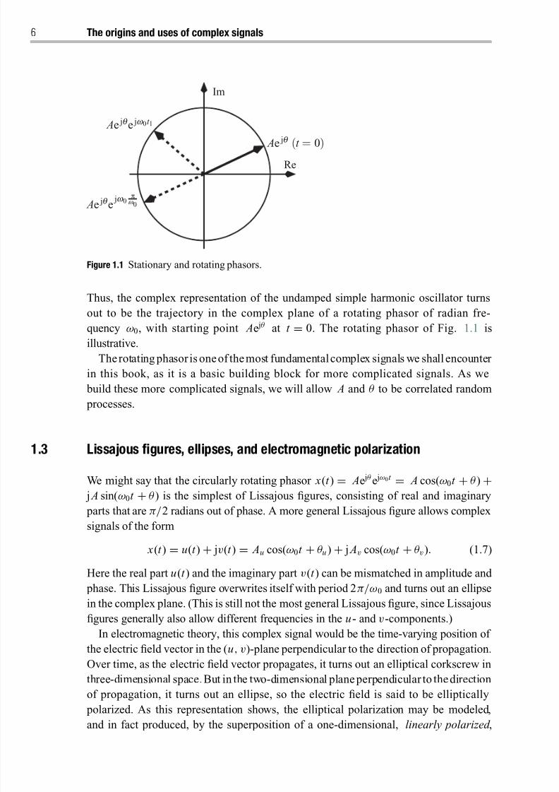
Figure 1.1 Stationary and rotating phasors.
Thus, the complex representation of the undamped simple harmonic oscillator turns
out to be the trajectory in the complex plane of a rotating phasor of radian fre-
quency ω0, with starting point Ae jθ at t = 0. The rotating phasor of Fig. 1.1 is
illustrative.
Therotating phasor is oneof themost fundamentalcomplex signals we shall encounter
in this book, as it is a basic building block for more complicated signals. As we
build these more complicated signals, we will allow A and θ to be correlated random
processes.
1.3 Lissajous figures, ellipses, and electromagnetic polarization
We might say that the circularly rotating phasor x(t ) = Ae jθ e jω0t = A cos(ω0t + θ ) + j A sin(ω0t + θ ) is the simplest of Lissajous figures, consisting of real and imaginary
parts that are π/2 radians out of phase. A more general Lissajous figure allows complex
signals of the form
x(t ) = u(t ) + jv(t ) = Au cos(ω0t + θ u) + j Av cos(ω0t + θ v). (1.7)Here the real part u(t ) and the imaginary part v(t ) can be mismatched in amplitude and
phase. This Lissajous figure overwrites itself with period 2π/ω0 and turns out an ellipse
in the complex plane. (This is still not the most general Lissajous figure, since Lissajous
figures generally also allow different frequencies in the u- and v-components.)
In electromagnetic theory, this complex signal would be the time-varying position of
the electric field vector in the (u, v)-plane perpendicular to the direction of propagation.
Over time, as the electric field vector propagates, it turns out an elliptical corkscrew in
three-dimensional space. But in the two-dimensional planeperpendicular to thedirection
of propagation, it turns out an ellipse, so the electric field is said to be elliptically polarized. As this representation shows, the elliptical polarization may be modeled,
and in fact produced, by the superposition of a one-dimensional, linearly polarized ,
8/21/2019 Statistical Signal Processing of Complex-Valued Data.pdf
http://slidepdf.com/reader/full/statistical-signal-processing-of-complex-valued-datapdf 29/330
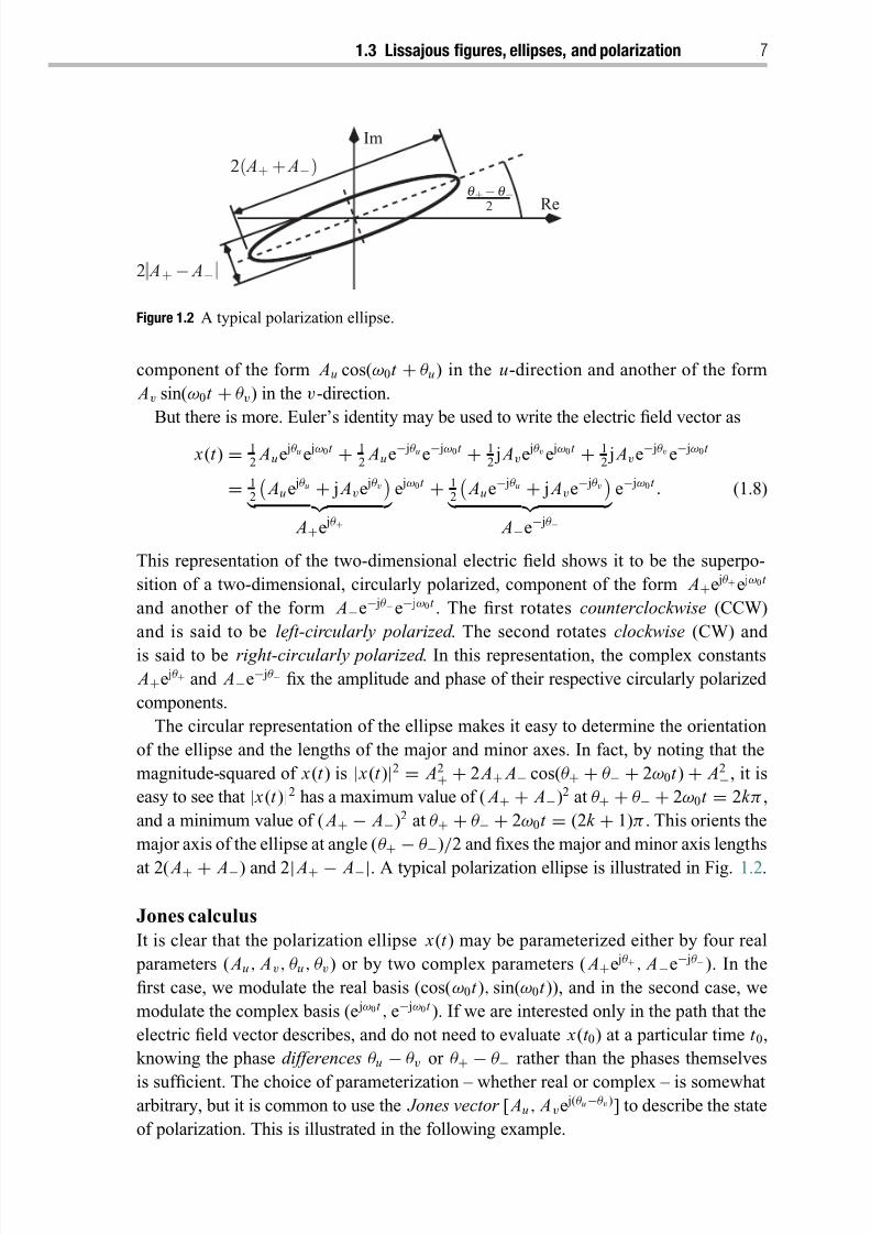
1.3 Lissajous figures, ellipses, and polarization 7
Re
Im
2( A+ + A−)
q+− q−2
2 A+− A−
Figure 1.2 A typical polarization ellipse.
component of the form Au cos(ω0t + θ u) in the u-direction and another of the form
Av sin(ω0t + θ v) in the v-direction.
But there is more. Euler’s identity may be used to write the electric field vector as
x(t ) = 12 Aue jθ u e jω0t + 1
2 Aue− jθ u e− jω0t + 1
2 j Ave jθ v e jω0t + 1
2 j Ave− jθ v e− jω0t
= 12
Aue jθ u + j Ave jθ v
A+e jθ +
e jω0t + 12
Aue− jθ u + j Ave− jθ v
A−e− jθ −
e− jω0t . (1.8)
This representation of the two-dimensional electric field shows it to be the superpo-
sition of a two-dimensional, circularly polarized, component of the form A+e jθ +e jω0t
and another of the form A−e− jθ −e− jω0t . The first rotates counterclockwise (CCW)
and is said to be left-circularly polarized . The second rotates clockwise (CW) and
is said to be right-circularly polarized . In this representation, the complex constants
A+e jθ + and A−e− jθ − fix the amplitude and phase of their respective circularly polarized
components.
The circular representation of the ellipse makes it easy to determine the orientation
of the ellipse and the lengths of the major and minor axes. In fact, by noting that the
magnitude-squared of x(t ) is | x(t )|2 = A2+ + 2 A+ A− cos(θ + + θ − + 2ω0t ) + A2
−, it is
easy to see that | x(t )|2 has a maximum value of ( A+ + A−)2 at θ + + θ − + 2ω0t = 2k π ,
and a minimum value of ( A+ − A−)2 at θ + + θ − + 2ω0t = (2k + 1)π . This orients the
major axis of the ellipse at angle (θ +−
θ −)/2 and fixes the major and minor axis lengths
at 2( A+ + A−) and 2| A+ − A−|. A typical polarization ellipse is illustrated in Fig. 1.2.
Jones calculus
It is clear that the polarization ellipse x(t ) may be parameterized either by four real
parameters ( Au , Av, θ u , θ v) or by two complex parameters ( A+e jθ +, A−e− jθ −). In the
first case, we modulate the real basis (cos(ω0t ), sin(ω0t )), and in the second case, we
modulate the complex basis (e jω0t , e− jω0t ). If we are interested only in the path that the
electric field vector describes, and do not need to evaluate x(t 0) at a particular time t 0,
knowing the phase differences θ u − θ v or θ + − θ − rather than the phases themselves
is sufficient. The choice of parameterization – whether real or complex – is somewhatarbitrary, but it is common to use the Jones vector [ Au , Ave j(θ u−θ v)] to describe the state
of polarization. This is illustrated in the following example.
8/21/2019 Statistical Signal Processing of Complex-Valued Data.pdf
http://slidepdf.com/reader/full/statistical-signal-processing-of-complex-valued-datapdf 30/330
8 The origins and uses of complex signals
Example 1.1. The Jones vectors for four basic states of polarization are (note that we do
not follow the convention of normalizing Jones vectors to unit norm):
10←→ x(t ) = cos(ω0t ) horizontal, linear polarization,
0
1
←→ x(t ) = j cos(ω0t ) vertical, linear polarization,
1
j
←→ x(t ) = e jω0t CCW (left-) circular polarization,
1
− j
←→ x(t ) = e− jω0t CW (right-) circular polarization.
Various polarization filters can be coded with two-by-two complex matrices that selec-
tively pass components of the polarization. For example, consider these two polarization
filters, and their corresponding Jones matrices:1 0
0 0
horizontal, linear polarizer ,
1
2
1 − j
j 1
CCW (left-)circular polarizer .
The first of these passes horizontal linear polarization and rejects vertical linear polariza-tion. Such polarizers are used to reduce vertically polarized glare in Polaroid sunglasses.
The second passes CCW circular polarization and rejects CW circular polarization. And
so on.
1.4 Complex modulation, the Hilbert transform, and complexanalytic signals
When analyzing the damped harmonic oscillator or the elliptically polarized electric
field, the appropriate complex representations present themselves naturally. We now
establish that this is so, as well, in the theory of modulation. Here the game is to
modulate a baseband , information-bearing, signal onto a passband carrier signal that
can be radiated from a real antenna onto a real channel. When the aim is to transmit
information from here to there, then the channel may be “air,” cable, or fiber. When the
aim is to transmit information from now to then, then the channel may be a magnetic
recording channel.
Actually, since a sinusoidal carrier signal can be modulated in amplitude and phase,the game is to modulate two information-bearing signals onto a carrier, suggesting again
that one complex signal might serve to represent these two real signals and provide
insight into how they should be designed. In fact, as we shall see, without the notion of
8/21/2019 Statistical Signal Processing of Complex-Valued Data.pdf
http://slidepdf.com/reader/full/statistical-signal-processing-of-complex-valued-datapdf 31/330
1.4 Complex modulation and analytic signals 9
a complex analytic signal , electrical engineers might never have discovered the Hilbert
transform and single-sideband (SSB) modulation as the most spectrally efficient way
to modulate one real channel of baseband information onto a passband carrier. Thus
modulation theory provides the proper context for the study of the Hilbert transform and
complex analytic signals.
1.4.1 Complex modulation using the complex envelope
Let us begin with two real information-bearing signals u(t )and v(t ), whicharecombined
in a complex baseband signal as
x(t ) = u(t ) + jv(t )
= A(t )e jθ (t ) = A(t )cos θ (t ) + j A(t )sin θ (t ). (1.9)
The amplitude A(t ) and phase θ (t ) are real. We take u(t ) and v(t ) to be lowpass signals
with Fourier transforms supported on a baseband interval of − < ω < . The repre-
sentation A(t )e jθ (t ) is a generalization of the stationary phasor, wherein the fixed radius
and angle of a phasor are replaced by a time-varying radius and angle. It is a simple
matter to go back and forth between x (t ) and (u(t ), v(t )) and ( A(t ), θ (t )).
From x (t ) we propose to construct the real passband signal
p(t )=
Re{ x(t )e jω0t
} = A(t )cos(ω0t
+θ (t ))
=u(t )cos(ω0t )
−v(t )sin(ω0t ). (1.10)
In accordance with standard communications terminology, we call x(t ) the complex
baseband signal or complex envelopeof p(t ), A(t )and θ (t ) the amplitude and phase of the
complex envelope, and u(t ) and v(t ) the in-phase and quadrature(-phase) components.
The term “quadrature component” refers to the fact that it is in phase quadrature (+π/2
out of phase) with respect to the in-phase component.
We say the complex envelope x (t ) complex-modulates the complex carrier e jω0t , when
what we really mean is that the real amplitude and phase ( A(t ), θ (t )) real-modulate the
amplitude and phase of the real carrier cos(ω0t ); or the in-phase and quadrature signals
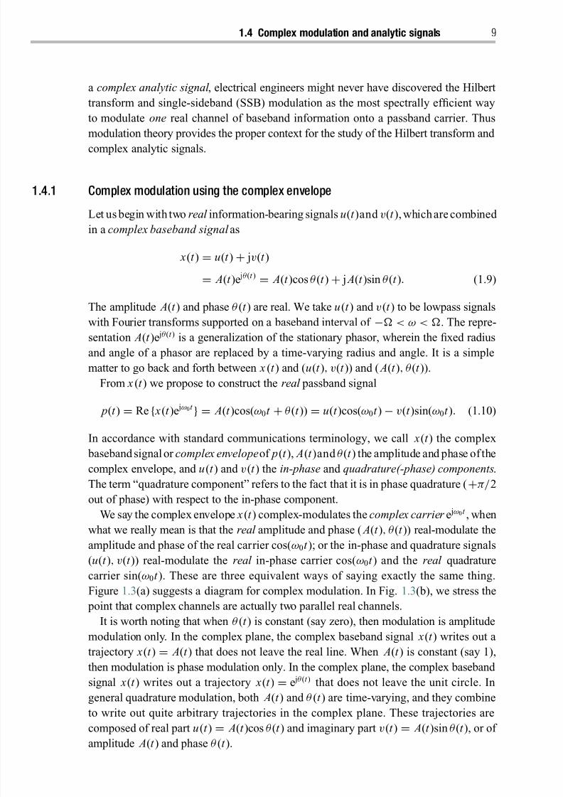
(u(t ), v(t )) real-modulate the real in-phase carrier cos(ω0t ) and the real quadraturecarrier sin(ω0t ). These are three equivalent ways of saying exactly the same thing.
Figure 1.3(a) suggests a diagram for complex modulation. In Fig. 1.3( b), we stress the
point that complex channels are actually two parallel real channels.
It is worth noting that when θ (t ) is constant (say zero), then modulation is amplitude
modulation only. In the complex plane, the complex baseband signal x(t ) writes out a
trajectory x(t ) = A(t ) that does not leave the real line. When A(t ) is constant (say 1),
then modulation is phase modulation only. In the complex plane, the complex baseband
signal x(t ) writes out a trajectory x(t ) = e jθ (t ) that does not leave the unit circle. In
general quadrature modulation, both A(t ) and θ (t ) are time-varying, and they combineto write out quite arbitrary trajectories in the complex plane. These trajectories are
composed of real part u(t ) = A(t )cos θ (t ) and imaginary part v(t ) = A(t )sin θ (t ), or of
amplitude A(t ) and phase θ (t ).
8/21/2019 Statistical Signal Processing of Complex-Valued Data.pdf
http://slidepdf.com/reader/full/statistical-signal-processing-of-complex-valued-datapdf 32/330
10 The origins and uses of complex signals
(b)
Re
(a)
v(t )
u(t )
(t ) p(t )
e jw 0t
sin ( )w 0t
p(t )
cos (w 0t )
Figure 1.3 (a) Complex and (b) quadrature modulation.
w 0
Im X (w )
Re X (w )
Im P (w )
w 0
−w 0 w
Re P (w )
w
−w 0
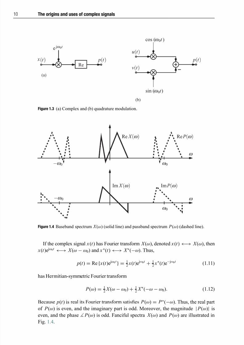
Figure 1.4 Baseband spectrum X (ω) (solid line) and passband spectrum P (ω) (dashed line).
If the complex signal x (t ) has Fourier transform X (ω), denoted x (t ) ←→ X (ω), then
x(t )e jω0t ←→ X (ω − ω0) and x ∗(t ) ←→ X ∗(−ω). Thus,
p(t ) = Re { x(t )e jω0t } = 12 x(t )e jω0t + 1
2 x∗(t )e− jω0t (1.11)
has Hermitian-symmetric Fourier transform
P (ω) = 12 X (ω − ω0) + 1
2 X ∗(−ω − ω0). (1.12)
Because p(t ) is real its Fourier transform satisfies P (ω) = P ∗(−ω). Thus, the real partof P (ω) is even, and the imaginary part is odd. Moreover, the magnitude | P (ω)| iseven, and the phase P (ω) is odd. Fanciful spectra X (ω) and P (ω) are illustrated in
Fig. 1.4.

8/21/2019 Statistical Signal Processing of Complex-Valued Data.pdf
http://slidepdf.com/reader/full/statistical-signal-processing-of-complex-valued-datapdf 33/330
1.4 Complex modulation and analytic signals 11
1.4.2 The Hilbert transform, phase splitter, and analytic signal
If the complex baseband signal x (t ) can be recovered from the passband signal p(t ), then
the two real channels u(t ) and v(t ) can be easily recovered as u(t )
=Re x(t )
= 12[ x(t )
+ x∗(t )] and v(t ) = Im x(t ) = [1/(2j)][ x(t ) − x∗(t )]. But how is x (t ) to be recovered from p(t )?
The real operator Re in the definition of p(t ) is applied to the complex signal x (t )e jω0t
and returns the real signal p(t ). Suppose there existed an inverse operator , i.e., a
linear, convolutional, complex operator, that could be applied to the real signal p(t )
and return the complex signal x(t )e jω0t . Then this complex signal could be complex-
demodulatedfor x(t ) = e− jω0t e jω0t x(t ). Thecomplexoperator would havetobedefined
by an impulse response φ(t ) ←→ (ω), whose Fourier transform (ω) were zero
for negative frequencies and 2 for positive frequencies, in order to return the signal
x(t )e jω
0t ←→ X (ω − ω0).This brings us to the Hilbert transform, the phase splitter, and the complex analytic
signal. The Hilbert transform of a signal p(t ) is denoted ˆ p(t ), and defined as the linear
shift-invariant operation
ˆ p(t ) = (h ∗ p)(t ) ∞−∞
h(t − τ ) p(τ )d τ ←→ ( H P )(ω) H (ω) P (ω) = ˆ P (ω).
(1.13)
The impulse response h(t ) and complex frequency response H (ω) of the Hilbert trans-
form are defined to be, for t ∈ IR and ω ∈ IR,
h(t ) = 1
π t ←→− j sgn(ω) = H (ω). (1.14)
Here sgn(ω) is the function
sgn(ω) =
1, ω > 0,
0, ω = 0,
−1, ω < 0.
(1.15)
So h(t ) is real and odd, and H (ω) is imaginary and odd. From the Hilbert transformh(t ) ←→ H (ω) we define the phase splitter
φ(t ) = δ(t ) + jh(t ) ←→ 1 − j2 sgn(ω) = 2(ω) = (ω). (1.16)
The complex frequency response of the phase splitter is (ω) = 2(ω), where (ω)
is the standard unit-step function. The convolution of the complex filter φ(t ) and the
real signal p(t ) produces the analytic signal y(t ) = p(t ) + j ˆ p(t ), with Fourier transform
identity
y(t )=
(φ∗
p)(t )=
p(t )+
j ˆ p(t )←→
P (ω)+
sgn(ω) P (ω)=
2( P )(ω)=
Y (ω).
(1.17)
Recall that the Fourier transform P (ω) of a real signal p(t ) has Hermitian sym-
metry P (−ω) = P ∗(ω), so P (ω) for ω < 0 is redundant. In the polar representation
8/21/2019 Statistical Signal Processing of Complex-Valued Data.pdf
http://slidepdf.com/reader/full/statistical-signal-processing-of-complex-valued-datapdf 34/330
12 The origins and uses of complex signals
P (ω) = B(ω)e j(ω), we have B (ω) = B(−ω) and (−ω) = −(ω). Therefore, the cor-
responding spectral representations for real p(t ) and complex analytic y(t ) are
p(t )=
∞
−∞ P (ω)e jωt d ω
2π =2
∞
0
B(ω)cos(ωt +
(ω))d ω
2π, (1.18)
y(t ) = ∞
0
2 P (ω)e jωt d ω
2π= 2
∞0
B(ω)e j(ωt +(ω)) d ω
2π. (1.19)
The analytic signal replaces the redundant two-sided spectral representation (1.18) by
theefficientone-sided representation (1.19). Equivalently, theanalytic signaluses a linear
combination of amplitude- and phase-modulated complex exponentials to represent
a linear combination of amplitude- and phase-modulated cosines. We might say the
analytic signal y(t ) is a bandwidth-efficient representation for its corresponding real
signal p(t ).
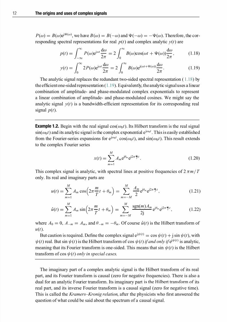
Example 1.2. Begin with the real signal cos(ω0t ). Its Hilbert transform is the real signal
sin(ω0t ) and its analytic signal is the complex exponential e jω0t . This is easily established
from the Fourier-series expansions for e jω0t , cos(ω0t ), and sin(ω0t ). This result extends
to the complex Fourier series
x(t ) = M
m=1
Ame jθ m e j2π mT
t . (1.20)
This complex signal is analytic, with spectral lines at positive frequencies of 2π m/ T
only. Its real and imaginary parts are
u(t ) = M
m=1
Am cos
2πm
T t + θ m
=
M m=− M
Am
2 e jθ m e j2π m
T t , (1.21)
u(t ) = M
m=1
Am sin
2πm
T t + θ m
=
M m=− M
sgn(m) Am
2j e jθ m e j2π m
T t , (1.22)
where A0 =
0, A−m =
Am
, and θ −m = −
θ m
. Of course u(t ) is the Hilbert transform of
u(t ).
But caution is required. Define the complex signal e jψ(t ) = cos ψ(t ) + j sin ψ(t ), with
ψ(t ) real. But sin ψ(t ) is the Hilbert transform of cos ψ(t ) if and only if e jψ(t ) is analytic,
meaning that its Fourier transform is one-sided. This means that sin ψ(t ) is the Hilbert
transform of cos ψ(t ) only in special cases.
The imaginary part of a complex analytic signal is the Hilbert transform of its real
part, and its Fourier transform is causal (zero for negative frequencies). There is also a
dual for an analytic Fourier transform. Its imaginary part is the Hilbert transform of itsreal part, and its inverse Fourier transform is a causal signal (zero for negative time).
This is called the Kramers–Kronig relation, after the physicists who first answered the
question of what could be said about the spectrum of a causal signal.

8/21/2019 Statistical Signal Processing of Complex-Valued Data.pdf
http://slidepdf.com/reader/full/statistical-signal-processing-of-complex-valued-datapdf 35/330
1.4 Complex modulation and analytic signals 13
(a)
(b)
p(t )v(
( (
t )( )
u(t )
x(t )
f(t )
(t )
jh
d e− jw 0t
cos w 0t
h
d
cos(w )0t
sin w 0t
Figure 1.5 Complex demodulation with the phase splitter: (a) one complex channel and (b) two
real channels.
1.4.3 Complex demodulation
Let’s recap. The output of the phase splitter applied to a passband signal p(t ) =Re { x(t )e jω0t } ←→ 1
2 X (ω − ω0) + 1
2 X ∗(−ω − ω0) = P (ω) is the analytic signal
y(t )=
(φ∗
p)(t )←→
( P )(ω)=
2( P )(ω)=
Y (ω). (1.23)
Under the assumption that the bandwidth of the spectrum X (ω) satisfies < ω0, we
have
Y (ω) =
X (ω − ω0), ω > 0,
0, ω ≤ 0.(1.24)
From here, we only need to shift y (t ) down to baseband to obtain the complex baseband
signal
x(t )=
y(t )e− jω0t
=(φ
∗ p)(t )e− jω0t
←→2( P )(ω
+ω0)
= X (ω). (1.25)
Two diagrams of a complex demodulator are shown in Fig. 1.5.
The Hilbert transform is an idealized convolution operator that can only be approx-
imated in practice. The usual approach to approximating it is to complex-demodulate
8/21/2019 Statistical Signal Processing of Complex-Valued Data.pdf
http://slidepdf.com/reader/full/statistical-signal-processing-of-complex-valued-datapdf 36/330
14 The origins and uses of complex signals
p(t ) as
e− jω0t p(t ) ←→ P (ω + ω0) = 12 X (ω) + 1
2 X ∗(−ω − 2ω0). (1.26)
Again, under the assumption that X (ω) is bandlimited, this demodulated signal may belowpass-filtered (with cutoff frequency ) for x(t ) ←→ X (ω). Of course there are no
ideal lowpass filters, so either the Hilbert transform is approximated and followed by a
complex demodulator, or a complex demodulator is followed by an approximate lowpass
filter.
Evidently, in the case of a complex bandlimited baseband signalmodulating a complex
carrier, a phase splitter followed by a complex demodulator is equivalent to a complex
demodulator followed by a lowpass filter. But how general is this? Bedrosian’s theorem
answers this question.
1.4.4 Bedrosian’s theorem: the Hilbert transform of a product
Let u(t ) = u1(t )u2(t ) be a product signal and let u(t ) denote the Hilbert transform of this
product. If U 1(ω) = 0 for |ω| > and U 2(ω) = 0 for |ω| < , then u(t ) = u1(t )u2(t ).
That is, the lowpass, slowly varying, factor may be regarded as constant when calculating
the Hilbert transform. The proof is a frequency-domain proof:
( H (U 1 ∗ U 2))(ω) = − j sgn(ω)(U 1 ∗ U 2)(ω)
= − j ∞−∞ U 1(ν)U 2(ω − ν)sgn(ω)
d ν
2π
= − j
∞−∞
U 1(ν)U 2(ω − ν)sgn(ω − ν) d ν
2π
= (U 1 ∗ ( HU 2))(ω). (1.27)
Actually, this proof is not as simple as it looks. It depends on the fact that sgn(ω − ν) =sgn(ω) over the range of values ν for which the integrand is nonzero.
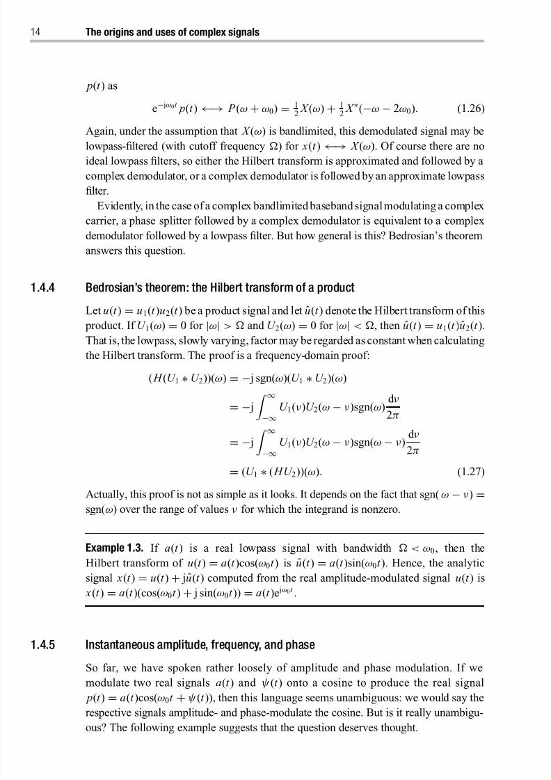
Example 1.3. If a(t ) is a real lowpass signal with bandwidth < ω0, then theHilbert transform of u(t ) = a(t )cos(ω0t ) is u(t ) = a(t )sin(ω0t ). Hence, the analytic
signal x(t ) = u(t ) + ju(t ) computed from the real amplitude-modulated signal u(t ) is
x(t ) = a(t )(cos(ω0t ) + j sin(ω0t )) = a(t )e jω0t .
1.4.5 Instantaneous amplitude, frequency, and phase
So far, we have spoken rather loosely of amplitude and phase modulation. If we
modulate two real signals a(t ) and ψ(t ) onto a cosine to produce the real signal p(t ) = a(t )cos(ω0t + ψ(t )), then this language seems unambiguous: we would say the
respective signals amplitude- and phase-modulate the cosine. But is it really unambigu-
ous? The following example suggests that the question deserves thought.
8/21/2019 Statistical Signal Processing of Complex-Valued Data.pdf
http://slidepdf.com/reader/full/statistical-signal-processing-of-complex-valued-datapdf 37/330
1.4 Complex modulation and analytic signals 15
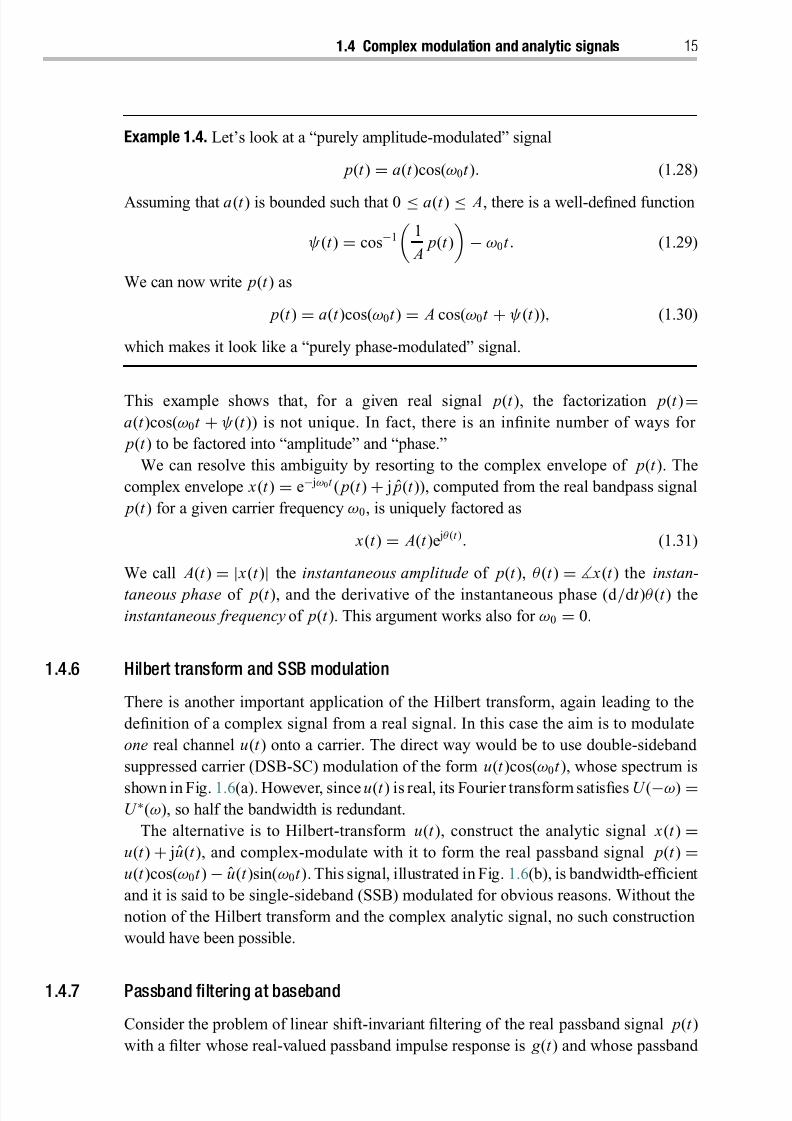
Example 1.4. Let’s look at a “purely amplitude-modulated” signal
p(t ) = a(t )cos(ω0t ). (1.28)
Assuming that a(t ) is bounded such that 0 ≤ a(t ) ≤ A, there is a well-defined function
ψ(t ) = cos−1
1
A p(t )
− ω0t . (1.29)
We can now write p(t ) as
p(t ) = a(t )cos(ω0t ) = A cos(ω0t + ψ(t )), (1.30)
which makes it look like a “purely phase-modulated” signal.
This example shows that, for a given real signal p(t ), the factorization p(t )=a(t )cos(ω0t + ψ(t )) is not unique. In fact, there is an infinite number of ways for
p(t ) to be factored into “amplitude” and “phase.”
We can resolve this ambiguity by resorting to the complex envelope of p(t ). The
complex envelope x(t ) = e− jω0t ( p(t ) + j ˆ p(t )), computed from the real bandpass signal
p(t ) for a given carrier frequency ω0, is uniquely factored as
x(t ) = A(t )e jθ (t ). (1.31)
We call A(t )
= | x(t )
| the instantaneous amplitude of p(t ), θ (t )
= x(t ) the instan-
taneous phase of p(t ), and the derivative of the instantaneous phase (d /d t )θ (t ) the
instantaneous frequency of p(t ). This argument works also for ω0 = 0.
1.4.6 Hilbert transform and SSB modulation
There is another important application of the Hilbert transform, again leading to the
definition of a complex signal from a real signal. In this case the aim is to modulate
one real channel u(t ) onto a carrier. The direct way would be to use double-sideband
suppressed carrier (DSB-SC) modulation of the form u(t )cos(ω0t ), whose spectrum is
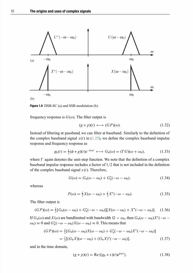
shown in Fig. 1.6(a). However, since u(t ) is real, its Fourier transform satisfies U (−ω) =U ∗(ω), so half the bandwidth is redundant.
The alternative is to Hilbert-transform u(t ), construct the analytic signal x(t ) =u(t ) + ju(t ), and complex-modulate with it to form the real passband signal p(t ) =u(t )cos(ω0t ) − u(t )sin(ω0t ). This signal, illustrated in Fig. 1.6( b), is bandwidth-efficient
and it is said to be single-sideband (SSB) modulated for obvious reasons. Without the
notion of the Hilbert transform and the complex analytic signal, no such construction
would have been possible.
1.4.7 Passband filtering at baseband
Consider the problem of linear shift-invariant filtering of the real passband signal p(t )
with a filter whose real-valued passband impulse response is g (t ) and whose passband
8/21/2019 Statistical Signal Processing of Complex-Valued Data.pdf
http://slidepdf.com/reader/full/statistical-signal-processing-of-complex-valued-datapdf 38/330
16 The origins and uses of complex signals
w
X (w −w 0) X ∗(−w −w 0)
U (w −w 0)U ∗(−w −w 0)
w
−w 0 w 0
w 0−w 0(a)
(b)
Figure 1.6 DSB-SC (a) and SSB modulation (b).
frequency response is G (ω). The filter output is
( g ∗ p)(t ) ←→ (G P )(ω). (1.32)
Instead of filtering at passband, we can filter at baseband. Similarly to the definition of
the complex baseband signal x(t ) in (1.25), we define the complex baseband impulse
response and frequency response as
g b(t ) = 12(φ ∗ g )(t )e− jω0t ←→ G b(ω) = (G )(ω + ω0), (1.33)
where again denotes the unit-step function. We note that the definition of a complex
baseband impulse response includes a factor of 1/2 that is not included in the definition
of the complex baseband signal x (t ). Therefore,
G (ω) = G b(ω − ω0) + G ∗ b(−ω − ω0), (1.34)
whereas
P (ω) = 12 X (ω − ω0) + 1
2 X ∗(−ω − ω0). (1.35)
The filter output is
(G P )(ω) = 12[G b(ω − ω0) + G ∗ b(−ω − ω0)][ X (ω − ω0) + X ∗(−ω − ω0)]. (1.36)
If G b(ω) and X (ω) are bandlimited with bandwidth < ω0, then G b(ω − ω0) X ∗(−ω −ω0) ≡ 0 and G ∗ b(−ω − ω0) X (ω − ω0) ≡ 0. This means that
(G P )(ω) = 12[G b(ω − ω0) X (ω − ω0) + G ∗ b(−ω − ω0) X ∗(−ω − ω0)]
= 12 [(G b X )(ω − ω0) + (G b X )∗(−ω − ω0)], (1.37)
and in the time domain,
( g ∗ p)(t ) = Re {( g b ∗ x)(t )e jω0t }. (1.38)
8/21/2019 Statistical Signal Processing of Complex-Valued Data.pdf
http://slidepdf.com/reader/full/statistical-signal-processing-of-complex-valued-datapdf 39/330
1.5 Complex signals for efficient FFT 17
Re
12e− jw 0t
(t )
g (t )
LPF
LPF
e− jw 0t
∗ ( g ∗ p)(t )
e jw 0t
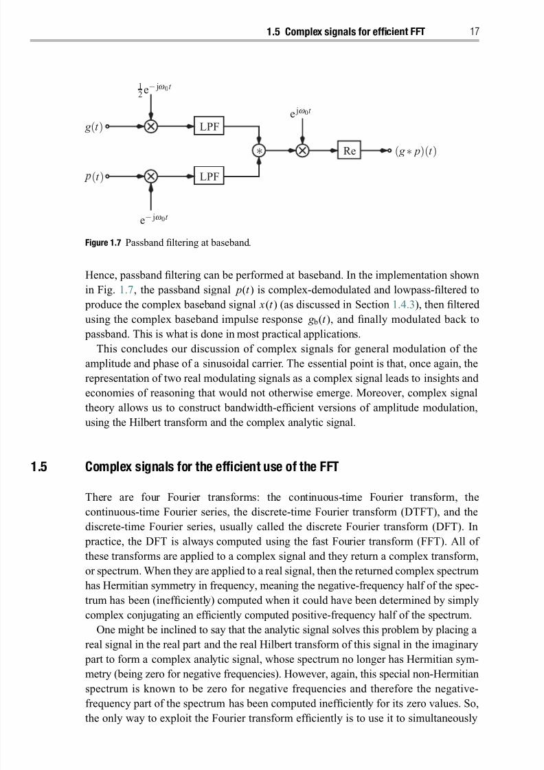
Figure 1.7 Passband filtering at baseband.
Hence, passband filtering can be performed at baseband. In the implementation shown
in Fig. 1.7, the passband signal p(t ) is complex-demodulated and lowpass-filtered to
produce the complex baseband signal x(t ) (as discussed in Section 1.4.3), then filtered
using the complex baseband impulse response g b(t ), and finally modulated back to
passband. This is what is done in most practical applications.
This concludes our discussion of complex signals for general modulation of the
amplitude and phase of a sinusoidal carrier. The essential point is that, once again, the
representation of two real modulating signals as a complex signal leads to insights and
economies of reasoning that would not otherwise emerge. Moreover, complex signal
theory allows us to construct bandwidth-efficient versions of amplitude modulation,using the Hilbert transform and the complex analytic signal.
1.5 Complex signals for the efficient use of the FFT
There are four Fourier transforms: the continuous-time Fourier transform, the
continuous-time Fourier series, the discrete-time Fourier transform (DTFT), and the
discrete-time Fourier series, usually called the discrete Fourier transform (DFT). In
practice, the DFT is always computed using the fast Fourier transform (FFT). All of these transforms are applied to a complex signal and they return a complex transform,
or spectrum. When they are applied to a real signal, then the returned complex spectrum
has Hermitian symmetry in frequency, meaning the negative-frequency half of the spec-
trum has been (inefficiently) computed when it could have been determined by simply
complex conjugating an efficiently computed positive-frequency half of the spectrum.
One might be inclined to say that the analytic signal solves this problem by placing a
real signal in the real part and the real Hilbert transform of this signal in the imaginary
part to form a complex analytic signal, whose spectrum no longer has Hermitian sym-
metry (being zero for negative frequencies). However, again, this special non-Hermitianspectrum is known to be zero for negative frequencies and therefore the negative-
frequency part of the spectrum has been computed inefficiently for its zero values. So,
the only way to exploit the Fourier transform efficiently is to use it to simultaneously
8/21/2019 Statistical Signal Processing of Complex-Valued Data.pdf
http://slidepdf.com/reader/full/statistical-signal-processing-of-complex-valued-datapdf 40/330
18 The origins and uses of complex signals
Fourier-transform two real signals that have been composed into the real and imaginary
parts of a complex signal, or to compose two subsampled versions of a length-2 N real
signal into the real and imaginary parts of a length- N complex signal.
Let’s first review the N -point DFT and its important identities. Then we will illustrate
its efficient use for transforming two real discrete-time signals of length N , and for
transforming a single real signal of length 2 N , using just one length- N DFT of a
complex signal. This treatment is adapted from Mitra (2006).
1.5.1 Complex DFT
We shall denote the DFT of the length- N sequence { x[n]} N −1n=0 by the length- N sequence
{ X [m]} N −1m=0 and establish the shorthand notation { x[n]} N −1
n=0 ←→ { X [m]} N −1m=0 . The mth
DFT coefficient X [m] is computed as
X [m] = N −1n=0
x[n]W −mn N , W N = e j2π/ N , (1.39)
and these DFT coefficients are inverted for the original signal as
x[n] = 1
N
N −1m=0
X [m]W mn N . (1.40)
The complex number W N
=e j2π/ N is an N th root of unity. When raised to the powers
n = 0, 1, . . . , N − 1, it visits all the N th roots of unity.
An important symmetry of the DFT is { x∗[n]} N −1n=0 ←→ { X ∗[( N − m) N ]} N −1
m=0 , which
reads “the DFT of a complex-conjugated sequence is the DFT of the original sequence,
complex-conjugated and cyclically reversed in frequency.” The notation ( N − m) N
stands for “ N − m modulo N ” so that X [( N ) N ] = X [0].
Now consider a length-2 N sequence { x[n]}2 N −1n=0 and its length-2 N DFT sequence
{ X [m]}2 N −1m=0 . Call {e[n] = x[2n]} N −1
n=0 the even polyphase component of x , and {o[n] = x[2n + 1]} N −1
n=0 the odd polyphase component of x . Their DFTs are {e[n]} N −1n=0 ←→
{ E [m]
} N −1m
=0 and
{o[n]
} N −1n
=0
←→ {O[m]
} N −1m
=0 . The DFT of
{ x[n]
}2 N −1n
=0 is, for m
=0, 1, . . . , 2 N − 1,
X [m] =2 N −1
n=0
x[n]W −mn2 N =
N −1n=0
e[n]W −mn N + W −m
N
N −1n=0
o[n]W −mn N
= E [(m) N ] + W −m N O[(m) N ]. (1.41)
That is, the 2 N -point DFT is computed from two N -point DFTs. In fact, this is the basis
of the decimation-in-time FFT.
1.5.2 Twofer: two real DFTs from one complex DFT
Begin with the two real length- N sequences {u[n]} N −1n=0 and {v[n]} N −1
n=0 . From them
form the complex signal { x[n] = u[n] + jv[n]} N −1n=0 . DFT this complex sequence
8/21/2019 Statistical Signal Processing of Complex-Valued Data.pdf
http://slidepdf.com/reader/full/statistical-signal-processing-of-complex-valued-datapdf 41/330
1.6 The bivariate Gaussian distribution 19
Od
FFT
Ev
N
N
N 2 N
2 N
2 N
W −m N
U X x
u
D j
↓ 2
↓ 2
E
O
Figure 1.8 Using one length- N complex DFT to compute the DFT for a length-2 N real signal.
for { x[n]} N −1n=0 ←→ { X [m]} N −1
m=0 . Now note that u[n] = 12( x[n] + x∗[n]), and v[n] =
[1/(2j)]( x[n] − x∗[n]). So for m = 0, 1, . . . , N − 1,
U [m] = 12
( X [m] + X ∗[( N − m) N ]), (1.42)
V [m] = 1
2j( X [m] − X ∗[( N − m) N ]). (1.43)
In this way, the N -point DFT is applied to a complex N -sequence x and efficiently
returns an N -point DFT sequence X , from which the DFTs for u and v are extracted
frequency-by-frequency.
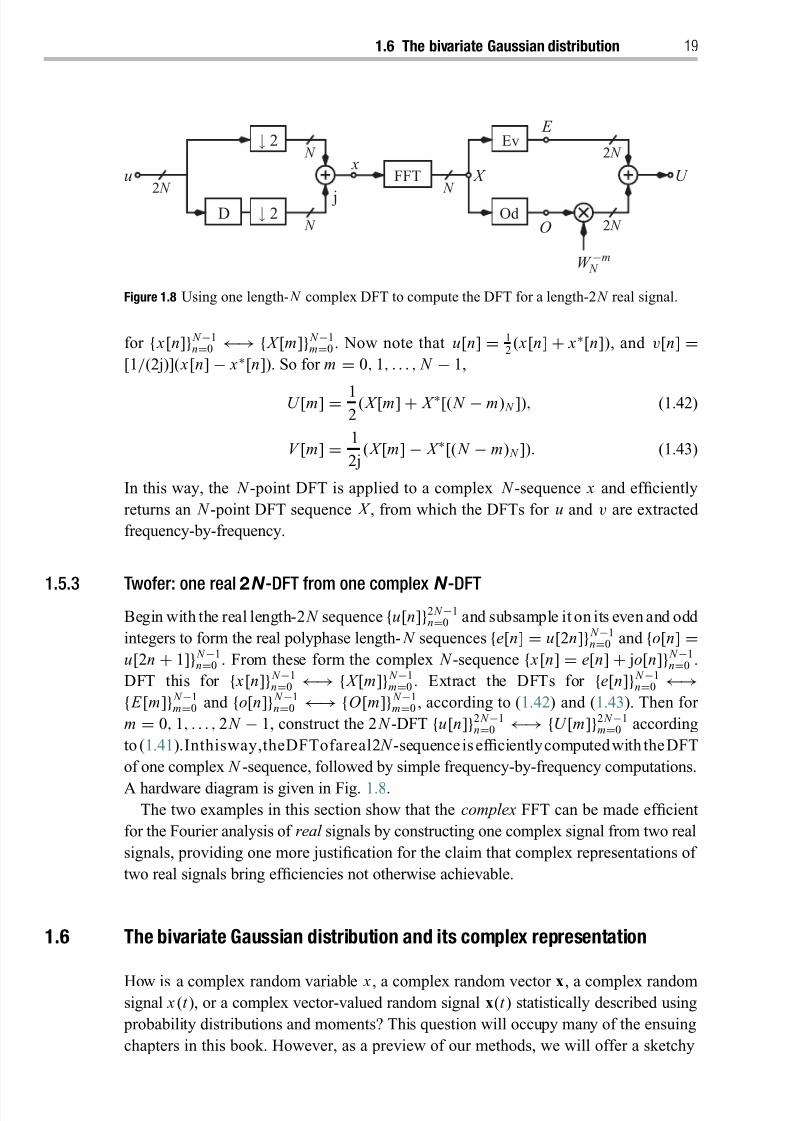
1.5.3 Twofer: one real 2N -DFT from one complex N -DFTBegin with the real length-2 N sequence {u[n]}2 N −1
n=0 and subsample it on its even and odd
integers to form the real polyphase length- N sequences {e[n] = u[2n]} N −1n=0 and {o[n] =
u[2n + 1]} N −1n=0 . From these form the complex N -sequence { x[n] = e[n] + jo[n]} N −1
n=0 .
DFT this for { x[n]} N −1n=0 ←→ { X [m]} N −1
m=0 . Extract the DFTs for {e[n]} N −1n=0 ←→
{ E [m]} N −1m=0 and {o[n]} N −1
n=0 ←→ {O[m]} N −1m=0 , according to (1.42) and (1.43). Then for
m = 0, 1, . . . , 2 N − 1, construct the 2 N -DFT {u[n]}2 N −1n=0 ←→ {U [m]}2 N −1
m=0 according
to (1.41).Inthisway,theDFTofareal2 N -sequenceis efficientlycomputedwith theDFT
of one complex N -sequence, followed by simple frequency-by-frequency computations.
A hardware diagram is given in Fig. 1.8.The two examples in this section show that the complex FFT can be made efficient
for the Fourier analysis of real signals by constructing one complex signal from two real
signals, providing one more justification for the claim that complex representations of
two real signals bring efficiencies not otherwise achievable.
1.6 The bivariate Gaussian distribution and its complex representation
How is a complex random variable x , a complex random vector x, a complex randomsignal x (t ), or a complex vector-valued random signal x(t ) statistically described using
probability distributions and moments? This question will occupy many of the ensuing
chapters in this book. However, as a preview of our methods, we will offer a sketchy

8/21/2019 Statistical Signal Processing of Complex-Valued Data.pdf
http://slidepdf.com/reader/full/statistical-signal-processing-of-complex-valued-datapdf 42/330
20 The origins and uses of complex signals
account of complex second-ordermoments andthe Gaussian probability density function
for the complex scalar x = u + jv. A more general account for vector-valued x will be
given in Chapter 2.
1.6.1 Bivariate Gaussian distribution
The real components u and v of the complex scalar random variable x = u + jv, which
may be arranged in a vector z = [u, v]T, are said to be bivariate Gaussian distributed,
with mean zero and covariance matrix R zz , if their joint probability density function
(pdf) is
puv(u, v) = 1
2π det1/2 R zz
exp
− 1
2
u v
R −1
zz
u
v
= 1
2π det1/2 R zz
exp− 1
2quv(u, v)
. (1.44)
Here the quadratic form quv(u, v) and the covariance matrix R zz of the composite vector
z are defined as follows:
quv(u, v) = u v
R −1 zz
u
v
, (1.45)
R zz = E (zzT) =
E (u2) E (uv)
E (vu) E (v2)=
Ruu
√ Ruu
√ Rvv ρuv√
Ruu
√ Rvv ρuv Rvv
. (1.46)
In the right-most parameterization of R zz , the terms are
Ruu = E (u2) variance of the random variable u,
Rvv = E (v2) variance of the random variable v,
Ruv =
Ruu
√ Rvv ρuv = E (uv) correlation of the random variables u, v,
ρuv = Ruv√
Ruu
√ Rvv
correlation coefficient of the random variables u, v.
As in (A1.38), the inverse of the covariance matrix R −1 zz may be factored as
R −1 zz =
1 0
−(√
Ruu /√
Rvv )ρuv 1
1/[ Ruu (1 − ρ2
uv)] 0
0 1/ Rvv
1 −(
√ Ruu /
√ Rvv )ρuv
0 1
.
(1.47)
Using (A1.3) we find det R zz = Ruu (1 − ρ2uv) Rvv , and from here the bivariate pdf
puv(u, v) may be written as
puv(u, v
) =1
(2π Ruu (1 − ρ2uv))1/2 exp− 1
2 Ruu (1 − ρ2uv) u − Ruu
√ Rvv
ρuv
v2
× 1
(2π Rvv )1/2 exp
− 1
2 Rvv
v2
. (1.48)

8/21/2019 Statistical Signal Processing of Complex-Valued Data.pdf
http://slidepdf.com/reader/full/statistical-signal-processing-of-complex-valued-datapdf 43/330
1.6 The bivariate Gaussian distribution 21
The term (√
Ruu /√
Rvv )ρuvv is the conditional mean estimator of u from v and e =u − (
√ Ruu /
√ Rvv )ρuv v is the error of this estimator. Thus the bivariate pdf p(u, v)
factors into a zero-mean Gaussian pdf for the error e, with variance Ruu (1 − ρ2uv), and
a zero-mean Gaussian pdf for v, with variance Rvv . The error e and v are independent.From u = r cos θ , v = r sin θ , d u d v = r d r d θ , it is possible to change variables and
obtain the pdf for the polar coordinates (r , θ )
pr θ (r , θ ) = r · puv(u, v)|u=r cos θ,v=r sin θ . (1.49)
From here it is possible to integrate over r to obtain the marginal pdf for θ and over θ
to obtain the marginal pdf for r . But this sequence of steps is so clumsy that it is hard
to find formulas in the literature for these marginal pdfs. There is an alternative, which
demonstrates again the power of complex representations.
1.6.2 Complex representation of the bivariate Gaussian distribution
Let’s code the real random variables u and v asu
v
= 1
2
1 1
− j j
x
x∗
. (1.50)
Then the quadratic form quv(u, v) in the definition of the bivariate Gaussian distribution
(1.45) may be written as
quv(u, v) = 14
x∗ x
1 j
1 − j
R −1
zz
1 1
− j j
x
x∗
= x∗ x
R −1 x x
x
x∗
, (1.51)
where the covariance matrix R x x and its inverse R −1 x x are
R x x = E x
x∗ x∗ x =
R x x
R x x
R∗ x x
R x x = 1 j
1 −
j R zz 1 1
− j j , (1.52)
R −1 x x = 1
4
1 j
1 − j
R −1
zz
1 1
− j j
= 1
R2 x x − | R x x |2
R x x − R x x
− R∗ x x R x x
. (1.53)
The new terms in this representation of the quadratic form quv(u, v) bear comment.
So let’s consider the elements of R x x . The variance term R x x is
R x x = E | x|2 = E [(u + jv)(u − jv)] = Ruu + Rvv + j0. (1.54)
This variance alone is an incomplete characterization for the bivariate pair (u, v), and it
carries no information at all about ρuv , the correlation coefficient between the random
variables u and v. But R x x contains another complex second-order moment
R x x = E x 2 = E [(u + jv)(u + jv)] = Ruu − Rvv + j2
Ruu
√ Rvv ρuv, (1.55)
8/21/2019 Statistical Signal Processing of Complex-Valued Data.pdf
http://slidepdf.com/reader/full/statistical-signal-processing-of-complex-valued-datapdf 44/330
22 The origins and uses of complex signals
which we will call the complementary variance. The complementary variance is the
correlation between x and its conjugate x∗. It is zero if and only if Ruu = Rvv and
ρuv = 0. This is the so-called proper case. All others are improper .
Now let’s introduce the complex correlation coefficient ρ between x and x∗ as
ρ = R x x
R x x
. (1.56)
Thus, we may write R x x = R x x ρ and R2 x x − | R x x |2 = R2
x x (1 − |ρ|2). Thecomplexcorre-
lation coefficient ρ = |ρ|e jψ satisfies |ρ| ≤ 1. If |ρ| = 1, then x = R x x R−1 x x x∗ = ρ x∗ =
e jψ x∗ with probability 1. Equivalent conditions for |ρ| = 1 are Ruu = 0, or Rvv = 0,
or ρuv = ±1. The first of these conditions makes the complex signal x purely imag-
inary and the second makes it real. The third condition means v = tan(ψ/2)u and
x =
[1+
j tan(ψ/2)]u. All these cases with |
ρ
| =1 are called maximally improper
because the support of the pdf for the complex random variable x degenerates into a line
in the complex plane.
There are three real parameters Ruu , Rvv , and ρuv required to determine the bivariate
pdf for (u, v), and these may be obtained from the three real values R x x , Re ρ, and
Im ρ (or alternatively, R x x , Re R x x , and Im R x x ) using the following inverse formulas of
(1.54) and (1.55):
Ruu = 12 R x x (1 + Re ρ), (1.57)
Rvv
= 12 R x x (1
−Re ρ), (1.58)
ρuv =Im ρ
1 − (Re ρ)2. (1.59)
Now, by replacing the quadratic form quv(u, v) in (1.44) with the expression (1.51),
and noting that det R x x = 4det R zz , we may record the complex representation of the
pdf for the bivariate Gaussian distribution or, equivalently, the pdf for complex x :
p x ( x) puv(u, v) = 1
π det1/2R x x
exp
− 1
2
x∗ x
R −1
x x
x
x∗
= 1π R x x
1 − |ρ|2
exp−| x |2
− Re (ρ x∗2
) R x x (1 − |ρ|2)
. (1.60)
This shows that the bivariate pdf for the real pair (u, v) can be written in terms of the
complex variable x . Yet the formula (1.60) is not what most people expect to see when
they talk about the pdf of a complex Gaussian random variable x . In fact, it is often
implicitly assumed that x is proper , i.e., ρ = 0 and x is not correlated with x ∗. Then the
pdf takes on the simple and much better-known form
p x ( x)
=
1
π R x x
exp−| x|2
R x x . (1.61)
But it is clear fromour development that (1.61) models only a special case of the bivariate
pdf for (u, v) where Ruu = Rvv and ρuv = 0. In general, we need to incorporate both the
variance R x x and the complementary variance R x x = R x x ρ. That is, even in this very
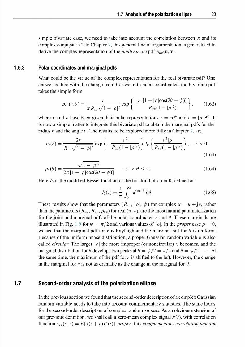
8/21/2019 Statistical Signal Processing of Complex-Valued Data.pdf
http://slidepdf.com/reader/full/statistical-signal-processing-of-complex-valued-datapdf 45/330
1.7 Analysis of the polarization ellipse 23
simple bivariate case, we need to take into account the correlation between x and its
complex conjugate x ∗. In Chapter 2, this general line of argumentation is generalized to
derive the complex representation of the multivariate pdf puv(u, v).
1.6.3 Polar coordinates and marginal pdfs
What could be the virtue of the complex representation for the real bivariate pdf? One
answer is this: with the change from Cartesian to polar coordinates, the bivariate pdf
takes the simple form
pr θ (r , θ ) = r
π R x x
1 − |ρ|2
exp
−r 2[1 − |ρ|cos(2θ − ψ)]
R x x (1 − |ρ|2)
, (1.62)
where x and ρ have been given their polar representations x =
r e jθ and ρ = |
ρ
|e jψ . It
is now a simple matter to integrate this bivariate pdf to obtain the marginal pdfs for the
radius r and the angle θ . The results, to be explored more fully in Chapter 2, are
pr (r ) = 2r
R x x
1 − |ρ|2
exp
− r 2
R x x (1 − |ρ|2)
I 0
r 2|ρ|
R x x (1 − |ρ|2)
, r > 0,
(1.63)
pθ (θ ) =
1 − |ρ|22π[1 − |ρ|cos(2θ − ψ)]
, −π < θ ≤ π. (1.64)
Here I 0 is the modified Bessel function of the first kind of order 0, defined as
I 0( z ) = 1
π
π
0
e z cos θ d θ. (1.65)
These results show that the parameters ( R x x , |ρ|, ψ) for complex x = u + jv, rather
than the parameters ( Ruu , Rvv , ρuv) for real (u, v), are the most natural parameterization
for the joint and marginal pdfs of the polar coordinates r and θ . These marginals are
illustrated in Fig. 1.9 for ψ = π/2 and various values of |ρ|. In the proper case ρ = 0,
we see that the marginal pdf for r is Rayleigh and the marginal pdf for θ is uniform.
Because of the uniform phase distribution, a proper Gaussian random variable is also
called circular . The larger |ρ| the more improper (or noncircular) x becomes, and themarginal distribution for θ develops two peaks at θ = ψ/2 = π/4 and θ = ψ/2 − π . At
the same time, the maximum of the pdf for r is shifted to the left. However, the change
in the marginal for r is not as dramatic as the change in the marginal for θ .
1.7 Second-order analysis of the polarization ellipse
In the previous section we found that thesecond-order description of a complex Gaussian
random variable needs to take into account complementary statistics. The same holdsfor the second-order description of complex random signals. As an obvious extension of
our previous definition, we shall call a zero-mean complex signal x (t ), with correlation
function r x x (t , τ ) = E [ x(t + τ ) x∗(t )], proper if its complementary correlation function
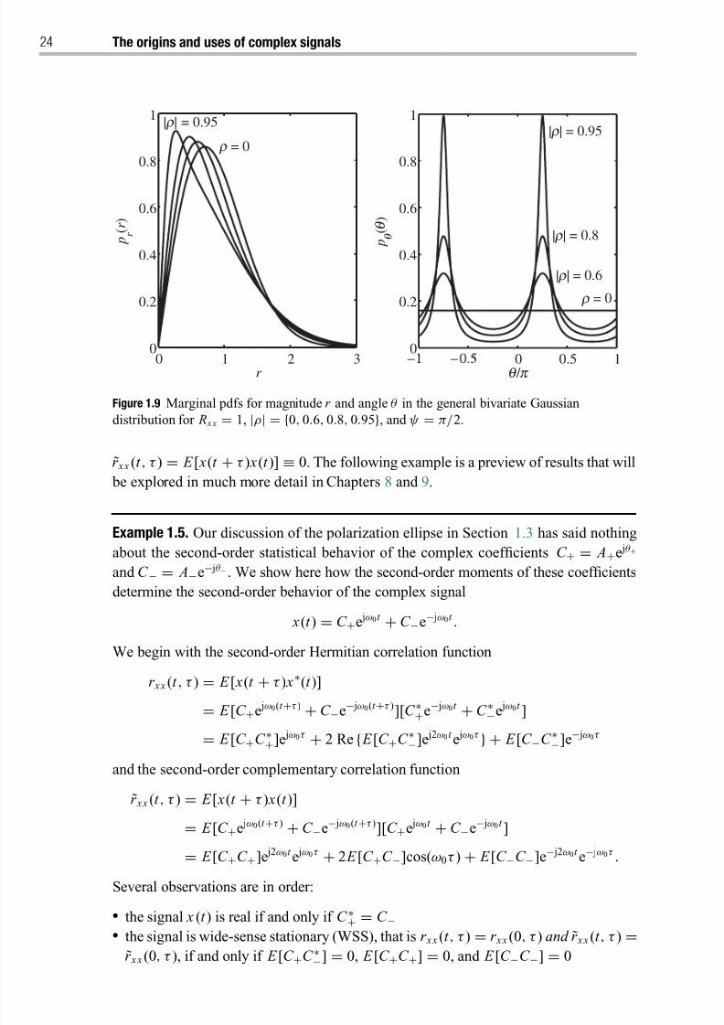
8/21/2019 Statistical Signal Processing of Complex-Valued Data.pdf
http://slidepdf.com/reader/full/statistical-signal-processing-of-complex-valued-datapdf 46/330
24 The origins and uses of complex signals
0 1 2 30
0.2
0.4
0.6
0.8
1
p r
( r )
r 0 0.5 1
0
0.2
0.4
0.6
0.8
1
p q
( q )
q / p
|r| = 0.6
|r| = 0.95
|r| = 0.8
r = 0
|r| = 0.95
r = 0
Figure 1.9 Marginal pdfs for magnitude r and angle θ in the general bivariate Gaussian
distribution for R x x = 1, |ρ| = {0, 0.6, 0.8, 0.95}, and ψ = π/2.
r x x (t , τ ) = E [ x(t + τ ) x(t )] ≡ 0. The following example is a preview of results that will
be explored in much more detail in Chapters 8 and 9.
Example 1.5. Our discussion of the polarization ellipse in Section 1.3 has said nothingabout the second-order statistical behavior of the complex coefficients C + = A+e jθ +
and C − = A−e− jθ − . We show here how the second-order moments of these coefficients
determine the second-order behavior of the complex signal
x(t ) = C +e jω0t + C −e− jω0t .
We begin with the second-order Hermitian correlation function
r x x (t , τ ) = E [ x(t + τ ) x∗(t )]
= E [C +e
jω0(t
+τ )
+ C −e− jω0(t
+τ )
][C ∗+e− jω0t
+ C ∗−e
jω0t
]= E [C +C ∗+]e jω0τ + 2 Re { E [C +C ∗−]e j2ω0t e jω0τ } + E [C −C ∗−]e− jω0τ
and the second-order complementary correlation function
r x x (t , τ ) = E [ x(t + τ ) x(t )]
= E [C +e jω0(t +τ ) + C −e− jω0(t +τ )][C +e jω0t + C −e− jω0t ]
= E [C +C +]e j2ω0t e jω0τ + 2 E [C +C −]cos(ω0τ ) + E [C −C −]e− j2ω0t e− jω0τ .
Several observations are in order:
the signal x (t ) is real if and only if C ∗+ = C − the signal is wide-sense stationary (WSS), that is r x x (t , τ ) = r x x (0, τ ) and r x x (t , τ ) =
r x x (0, τ ), if and only if E [C +C ∗−] = 0, E [C +C +] = 0, and E [C −C −] = 0

8/21/2019 Statistical Signal Processing of Complex-Valued Data.pdf
http://slidepdf.com/reader/full/statistical-signal-processing-of-complex-valued-datapdf 47/330
1.8 Mathematical framework 25
the signal is proper, that is r x x (t , τ ) = 0, if and only if E [C +C +] = 0, E [C +C −] = 0,
and E [C −C −] = 0 the signal isproperand WSS ifand only if E [C +C ∗−] = 0, E [C +C +] = 0, E [C +C −] =
0, and E [C −
C −
]=
0 the signal cannot be nonzero, real, and proper, because C ∗+ = C − makes E [C +C −] =
E [C +C ∗+] > 0
So a signal can be proper and WSS, proper and nonstationary, improper and WSS, or
improper and nonstationary. If the signal is real then it is improper, but it can be WSS
or nonstationary.
1.8 Mathematical framework
This chapter has shown that there are conceptual differences between one complex signal
and two real signals. In this section, we will explain why there are also mathematical
differences. This will allow us to provide a first glimpse at the mathematical framework
that underpins much of what is to come later in this book. Consider the simple C-linear
relationship between two complex scalars x = u + jv and y = a + jb:
y = kx . (1.66)
We may write this relationship in terms of real and imaginary parts asa
b
=
Re k −Im k
Im k Re k
M
u
v
. (1.67)
The 2 × 2 matrix M has a special structure and is determined by two real numbers Re k
and Im k . On the other hand, a general linear transformation on IR 2 is
a
b=
M 11 M 12
M 21 M 22 M
u
v, (1.68)
where all four elements of M may be chosen freely. This IR 2-linear expression is C-
linear, i.e., it can be expressed as y = kx , if and only if M 11 = M 22 and M 21 = − M 12. In
the more general case, where M 11 = M 22 and/or M 21 = − M 12, the complex equivalent
of (1.68) is the linear–conjugate-linear, or widely linear , transformation
y = k 1 x + k 2 x∗. (1.69)
Widely linear transformations depend linearly on x and its conjugate x ∗. The two com-
plex coefficients k 1 and k 2 have a one-to-one correspondence to the four real coefficients M 11, M 12, M 21, M 22, which we derive in Section 2.1.
Traditionally, widely linear transformations have been employed only reluctantly.
If the IR 2-linear transformation (1.68) does not satisfy M 11 = M 22 and M 21 = − M 11,
8/21/2019 Statistical Signal Processing of Complex-Valued Data.pdf
http://slidepdf.com/reader/full/statistical-signal-processing-of-complex-valued-datapdf 48/330
26 The origins and uses of complex signals
most people would prefer the IR 2-linear representation (1.68) over the C-widely linear
representation (1.69). As a matter of fact, in classical complex analysis, functions that
depend on x∗ are not even considered differentiable even if they are differentiable
when expressed as two-dimensional functions in terms of real and imaginary parts (seeAppendix 2). In this book, we aim to make the point that a complex representation is
not only feasible but also can be much more powerful and elegant, even if it leads to
expressions involving complex conjugates.
A key tool will be the augmented representation of widely linear transformations,
where we express (1.69) as y
y∗
=
k 1 k 2k ∗2 k ∗1
x
x∗
,
y=
K x. (1.70)
This representation utilizes the augmented vectors
y =
y
y∗
and x =
x
x∗
(1.71)
and the augmented matrix
K =
k 1 k 2k ∗2 k ∗1
. (1.72)
Augmented vectors and matrices are underlined. The augmented representation obvi-ously has some built-in redundancy but it will turn out to be very useful and convenient
as we develop the first- and second-order theories of improper signals. The space of
augmented complex vectors [ x, y]T, where y = x∗, is denoted C2∗, and it is isomorphic
to IR 2. However, C2∗ is only an IR-linear (or C-widely linear), but not a C-linear, subspace
of C 2. It satisfies all properties of a linear subspace except that it is not closed under
multiplication with a complex scalar α because α x∗ = (α x)∗. Similarly, augmented
matrices form a matrix algebra that is closed under addition, multiplication, inversion,
and multiplication with a real scalar but not under multiplication with a complex scalar.
We have already had a first exposure to augmented vectors and matrices in our discussion of thecomplex Gaussian distribution in Section 1.6. In fact, we now recognize
that the covariance matrix defined in (1.52) is
R x x = E x xH =
R x x R x x R∗
x x R x x
. (1.73)
This is the covariance matrix of the augmented vector x = [ x , x∗]T, and R x x itself is an
augmented matrix because R x x = R∗ x x . This is why we call R x x the augmented covari-
ance matrixof x . Theaugmentedcovariance matrix R x x is more than simply a convenient
way of keeping track of both the variance R x x = E | x|2 and the complementary variance R x x = E x 2. By combining R x x and R x x into R x x , we gain access to the large number of
results on 2 × 2 matrices. For instance, we know that any covariance matrix, including
R x x , must be positive semidefinite and thus have nonnegative determinant, det R x x ≥ 0.
8/21/2019 Statistical Signal Processing of Complex-Valued Data.pdf
http://slidepdf.com/reader/full/statistical-signal-processing-of-complex-valued-datapdf 49/330
1.9 A brief survey of applications 27
This immediately leads to | R x x |2 ≤ R2 x x , a simple upper bound on the magnitude of the
complementary variance.
1.9 A brief survey of applications
The following is a brief survey of a few applications of improper and noncircular com-
plex random signals, without any attempt at a complete bibliography. Our aim here
is to indicate the breadth of applications spanning areas as diverse as communica-
tions and oceanography. We apologize in advance to authors whose work has not been
included.
Currently, much of the research utilizing improper random signals concerns appli-
cations in communications. So what has sparked this recent interest in impropriety?
There is an important result (cf. Results 2.15 and 2.16) stating that wide-sense sta-
tionary analytic signals, and also complex baseband representations of wide-sense
stationary real bandpass signals, must be proper. On the other hand, nonstationary
analytic signals and complex baseband representations of nonstationary real bandpass
signals can be improper. In digital communications, thermal noise is assumed to be
wide-sense stationary, but the transmitted signals are nonstationary (in fact, as we will
discuss in Chapter 9, they are cyclostationary). This means that the analytic and com-
plex baseband representations of thermal noise are always proper, whereas the analytic
and complex baseband representations of the transmitted data signal are potentially
improper.
In optimum maximum-likelihood detection, only the noise is assigned statistical
properties. The likelihood function, which is the probability density function of the
received signal conditioned on the transmitted signal, is proper because the noise is
proper. Therefore, in maximum-likelihood detection, it is irrelevant whether or not the
transmitted signal is improper. The communications research until the 1990s focused
on optimal detection strategies based on maximum likelihood and was thus prone to
overlook the potential impropriety of the data signal.
However, when more complicated scenarios are considered, such as multiuser or
space–time communications, maximum likelihood is no longer a viable detection strat-egy because it is computationally too expensive. In these scenarios, detection is usually
based on suboptimum algorithms that are less complex to implement. Many of these
suboptimum detection algorithms do assign statistical properties to the signal. Hence,
the potentially improper nature of signals must be taken into account when design-
ing these detection algorithms. In mobile multiuser communications, this leads to a
significantly improved tradeoff between spectral efficiency and power consumption.
Important examples of digital modulation schemes that produce improper complex
baseband signals are Binary Phase Shift Keying (BPSK), Pulse Amplitude Modula-
tion (PAM), Gaussian Minimum Shift Keying (GMSK), Offset Quaternary Phase ShiftKeying (OQPSK), and baseband (but not passband) Orthogonal Frequency Division
Multiplexing (OFDM), which is commonly called Discrete Multitone (DMT). A small
sample of papers addressing these issues is Yoon and Leib (1997), Gelli et al . (2000),
8/21/2019 Statistical Signal Processing of Complex-Valued Data.pdf
http://slidepdf.com/reader/full/statistical-signal-processing-of-complex-valued-datapdf 50/330
28 The origins and uses of complex signals
Lampe et al . (2002), Gerstacker et al . (2003), Nilsson et al . (2003), Napolitano and
Tanda (2004), Witzke (2005), Buzzi et al . (2006), Jeon et al . (2006), Mirbagheri et al .
(2006), Chevalier and Pipon (2006), Taubock (2007), and Cacciapuoti et al . (2007).
Improper baseband communication signals can also arise due to imbalance between
their in-phase and quadrature (I/Q) components. This can be caused by amplifier or
receiver imperfections, or by communication channels that are not rotationally invariant.
If the in-phase and quadrature components of a signal are subject to different gains, or
if the phase-offset between them is not exactly 90◦, even rotationally invariant modula-
tion schemes such as Quaternary Phase Shift Keying (QPSK) become improper at the
receiver. I/Q imbalance degrades the signal-to-noise ratio and thus bit error rate per-
formance. Some papers proposing ways of compensating for I/Q imbalance in various
typesof communication systems include Anttila etal . (2008), Rykaczewski etal . (2008),
and Zou et al . (2008). Morgan (2006) and Morgan and Madsen (2006) present tech-
niques for wideband system identification when the system (e.g., a wideband wireless
communication channel) is not rotationally invariant.
Array processing is the generic term applied to processing the output of an array of
sensors. An important example of array processing is beamforming , which allows direc-
tional signal transmission or reception, either for radio or for sound waves. Besides the
perhaps obvious applications in radar, sonar, and wireless communications, array pro-
cessing is also employed in fields such as seismology, radio astronomy, and biomedicine.
Often the aim is to estimate the direction of arrival (DOA) of one or more signals of
interest impinging on a sensor array. If the signals of interest or the interference are
improper (as they would be if they originated, e.g., from a BPSK transmitter), this can
be exploited to achieve higher DOA resolution. Some papers addressing the adapta-
tion of array-processing algorithms to improper signals include Charge et al . (2001),
McWhorter and Schr eier (2003), Haardt and R oemer (2004), Delmas (2004), Chevalier
and Blin (2007), and R omer and Haardt (2009).
Another area where the theory of impropriety has led to important advances is
machine learning. Much interest is centered around independent component analysis
(ICA), which is a technique for separating a multivariate signal into additive components
that are as independent as possible. A typical application of ICA is to functional mag-
netic resonance imaging (fMRI), which measures neural activity in the brain or spinalcord. The fMRI signal is naturally modeled as a complex signal (see Adali and Calhoun
(2007) for an introduction to complex ICA applied to fMRI data). In the past, it has
been assumed that the fMRI signal is proper, when in fact it isn’t. As we will discuss in
Section 3.5, impropriety is even a desirable property because it enables the separation of
signals that would otherwise not be separable. The impropriety of the fMRI signal is now
recognized, and techniques for ICA of complex signals that exploit impropriety have
been proposed by DeLathauwer and DeMoor (2002), Eriksson and Koivunen (2006),
Adali et al . (2008), Novey and Adali (2008a,2008b), Li and Adali (2008), and Ollila
and Koivunen (2009), amongst others.Machine-learning techniques are often implemented using neural networks. Exam-
ples of neural-network implementations of signal processing algorithms utilizing com-
plementary statistics are given by Goh and Mandic (2007a, 2007b). A comprehensive
8/21/2019 Statistical Signal Processing of Complex-Valued Data.pdf
http://slidepdf.com/reader/full/statistical-signal-processing-of-complex-valued-datapdf 51/330
1.9 A brief survey of applications 29
account of complex-valued nonlinear adaptive filters is provided in the research mono-
graph by Mandic and Goh (2009).
The theory of impropriety has also found recent applications in acoustics (e.g.,
Rivet et al . (2007)) and optics. In optics, the standard correlation function is called
the phase-insensitive correlation, and the complementary correlation function is called
the phase-sensitive correlation. In a recent paper, Shapiro and Erkmen (2007) state
that “Optical coherence theory for the complex envelopes of passband fields has been
concerned, almost exclusively, with correlations that are all phase insensitive, despite
decades of theoretical and experimental work on the generation and applications of
light with phase-sensitive correlations. This paper begins the process of remedying that
deficiency . . . .” More details on the work with phase-sensitive light can be found in
Erkmen and Shapiro (2006) and the Ph.D. dissertation by Erkmen (2008). Maybe our
discussion of polarization analysis in Sections 8.4 and 9.4 can make a contribution to
this topic.
It is interesting to note that perhaps the first fields of research that recognized the
importance of the complementary correlation and made consistent use of complex
representations are oceanography and geophysics. The seminal paper by Mooers (1973),
buildingupon prior work by Gonella (1972), presentedtechniques for thecross-spectrum
analysisof bivariate time seriesby modeling them as complex-valued time series. Mooers
realized that the information in the standard correlation function – which he called the
inner-cross correlation – must be complemented by the complementary correlation
function – which he called the outer-cross correlation – to fully model the second-
order behavior of bivariate time series. He also recognized that the complex-valued
description yields the desirable property that coherences are invariant under coordinate
rotation. Moreover, testing for coherence between a pair of complex-valued time series
is significantly simplified compared with the r eal-valued descri ption. Early examples
using this work are the analysis of wind fields by Burt et al . (1974) and the interpretation
of ocean-current spectra by Calman (1978). Mooers’ work is still frequently cited today,
and it provides the basis for our discussion of polarization analysis in Section 8.4.
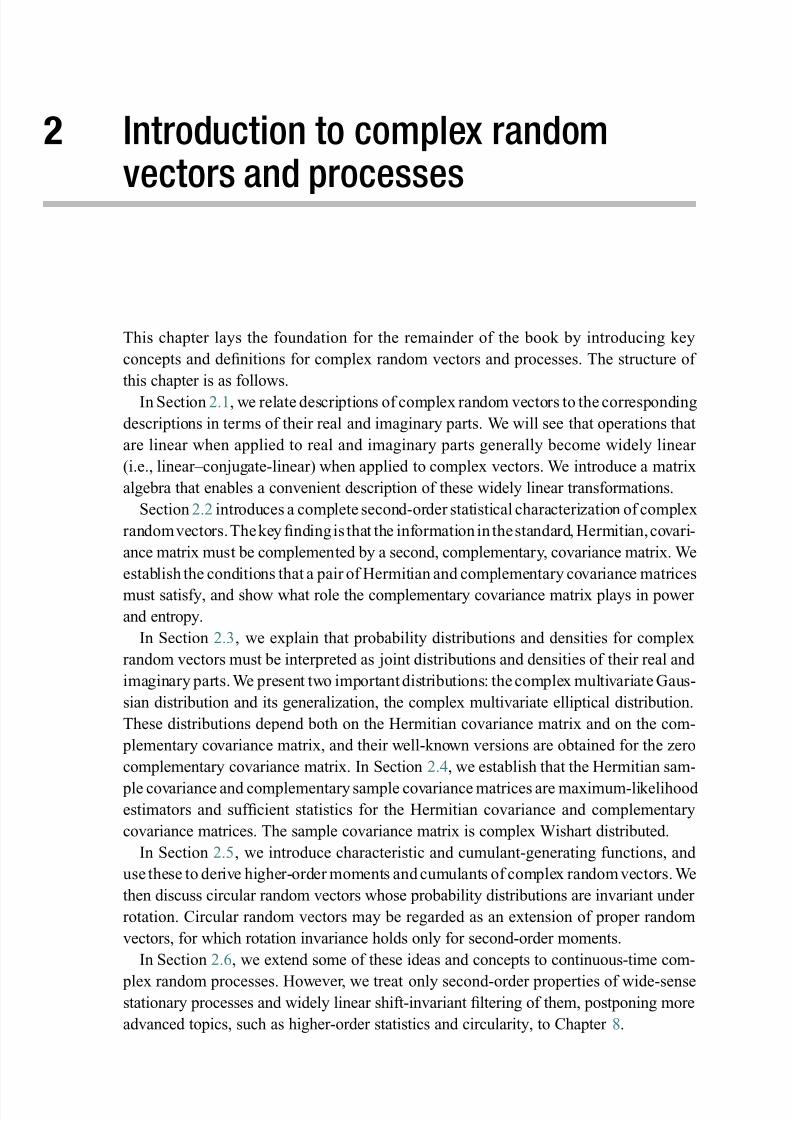
8/21/2019 Statistical Signal Processing of Complex-Valued Data.pdf
http://slidepdf.com/reader/full/statistical-signal-processing-of-complex-valued-datapdf 52/330
2 Introduction to complex randomvectors and processes
This chapter lays the foundation for the remainder of the book by introducing key
concepts and definitions for complex random vectors and processes. The structure of
this chapter is as follows.
In Section 2.1, we relate descriptions of complex random vectors to the corresponding
descriptions in terms of their real and imaginary parts. We will see that operations that
are linear when applied to real and imaginary parts generally become widely linear
(i.e., linear–conjugate-linear) when applied to complex vectors. We introduce a matrix
algebra that enables a convenient description of these widely linear transformations.
Section 2.2 introduces a complete second-order statistical characterization of complex
randomvectors.Thekey findingis that the information in thestandard, Hermitian,covari-
ance matrix must be complemented by a second, complementary, covariance matrix. We
establish the conditions that a pair of Hermitian and complementary covariance matrices
must satisfy, and show what role the complementary covariance matrix plays in power
and entropy.
In Section 2.3, we explain that probability distributions and densities for complex
random vectors must be interpreted as joint distributions and densities of their real and
imaginary parts. We present two important distributions: thecomplex multivariate Gaus-
sian distribution and its generalization, the complex multivariate elliptical distribution.
These distributions depend both on the Hermitian covariance matrix and on the com-
plementary covariance matrix, and their well-known versions are obtained for the zero
complementary covariance matrix. In Section 2.4, we establish that the Hermitian sam-
ple covariance and complementary sample covariance matrices are maximum-likelihood estimators and sufficient statistics for the Hermitian covariance and complementary
covariance matrices. The sample covariance matrix is complex Wishart distributed.
In Section 2.5, we introduce characteristic and cumulant-generating functions, and
use these to derive higher-order moments and cumulants of complex randomvectors. We
then discuss circular random vectors whose probability distributions are invariant under
rotation. Circular random vectors may be regarded as an extension of proper random
vectors, for which rotation invariance holds only for second-order moments.
In Section 2.6, we extend some of these ideas and concepts to continuous-time com-
plex random processes. However, we treat only second-order properties of wide-sensestationary processes and widely linear shift-invariant filtering of them, postponing more
advanced topics, such as higher-order statistics and circularity, to Chapter 8.

8/21/2019 Statistical Signal Processing of Complex-Valued Data.pdf
http://slidepdf.com/reader/full/statistical-signal-processing-of-complex-valued-datapdf 53/330
2.1 Real and complex descriptions 31
2.1 Connection between real and complex descriptions
Let be the sample space of a random experiment, and u: −→ IR n and v: −→ IR n
be two real random vectors defined on . From u and v we construct three closelyrelated vectors. The first is the real composite random vector z: −→ IR 2n, obtained
by stacking u on v:
z =
u
v
. (2.1)
The second vector is the complex random vector x: −→ Cn, obtained by composing
u and v into its real and imaginary parts:
x
=u
+ jv. (2.2)
The third vector is the complex augmented random vector x: −→ C2n∗ , obtained by
stacking x on top of its complex conjugate x∗:
x =
x
x∗
. (2.3)
The space of complex augmented vectors, whose bottom n entries are the complex
conjugates of the top n entries, is denoted by C2n∗ . Augmented vectors will always be
underlined.
The complex augmented vector x is related to the real composite vector z as
x = Tn z ⇐⇒ z = 12
THn x, (2.4)
where the real-to-complex transformation
Tn =
I jI
I − jI
∈ C2n×2n (2.5)
is unitary up to a factor of 2:
Tn TH
n = TH
n Tn = 2I. (2.6)
The complex augmented random vector x: −→ C2n∗ is obviously an equivalent redun-
dant representation of z: −→ IR 2n . But far from being a vice, this redundancy will
be turned into an evident virtue as we develop the algebra of improper complex random
vectors. Whenever the size of Tn is clear, we will drop the subscript n for economy.
2.1.1 Widely linear transformations
If a real linear transformation M
∈IR 2m×2n is applied to the composite real vector
z: −→ IR 2n , it yields a real composite vector w: −→ IR 2m ,
w =
a
b
=
M11 M12
M21 M22
u
v
= Mz, (2.7)
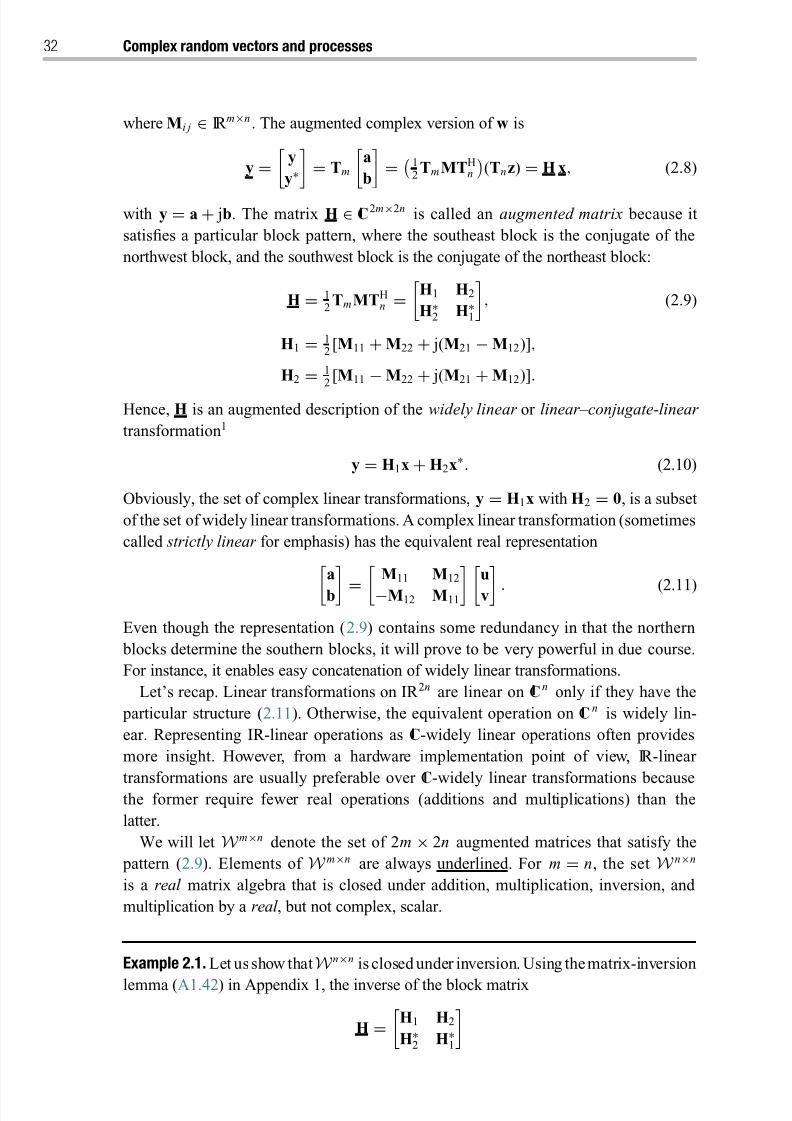
8/21/2019 Statistical Signal Processing of Complex-Valued Data.pdf
http://slidepdf.com/reader/full/statistical-signal-processing-of-complex-valued-datapdf 54/330
32 Complex random vectors and processes
where Mi j ∈ IR m×n . The augmented complex version of w is
y =
y
y∗= Tm
a
b=
12
Tm MTHn
(Tn z) = H x, (2.8)
with y = a + jb. The matrix H ∈ C2m×2n is called an augmented matrix because it
satisfies a particular block pattern, where the southeast block is the conjugate of the
northwest block, and the southwest block is the conjugate of the northeast block:
H = 12
Tm MTHn =
H1 H2
H∗2 H∗
1
, (2.9)
H1 = 12[M11 + M22 + j(M21 − M12)],
H2
= 12[M11
−M22
+ j(M21
+M12)].
Hence, H is an augmented description of the widely linear or linear–conjugate-linear
transformation1
y = H1x + H2x∗. (2.10)
Obviously, the set of complex linear transformations, y = H1x with H2 = 0, is a subset
of the set of widely linear transformations. A complex linear transformation (sometimes
called strictly linear for emphasis) has the equivalent real representation
a
b = M11 M12
−M12 M11 u
v . (2.11)
Even though the representation (2.9) contains some redundancy in that the northern
blocks determine the southern blocks, it will prove to be very powerful in due course.
For instance, it enables easy concatenation of widely linear transformations.
Let’s recap. Linear transformations on IR 2n are linear on Cn only if they have the
particular structure (2.11). Otherwise, the equivalent operation on Cn is widely lin-
ear. Representing IR-linear operations as C-widely linear operations often provides
more insight. However, from a hardware implementation point of view, IR-linear
transformations are usually preferable over C-widely linear transformations becausethe former require fewer real operations (additions and multiplications) than the
latter.
We will let W m×n denote the set of 2m × 2n augmented matrices that satisfy the
pattern (2.9). Elements of W m×n are always underlined. For m = n, the set W n×n
is a real matrix algebra that is closed under addition, multiplication, inversion, and
multiplication by a real , but not complex, scalar.
Example 2.1. Let usshow that
W n×n is closed under inversion. Using thematrix-inversion
lemma (A1.42) in Appendix 1, the inverse of the block matrix
H =
H1 H2
H∗2 H∗
1
8/21/2019 Statistical Signal Processing of Complex-Valued Data.pdf
http://slidepdf.com/reader/full/statistical-signal-processing-of-complex-valued-datapdf 55/330
2.1 Real and complex descriptions 33
can be calculated as
H−1 =
(H1 − H2H−∗1 H∗
2)−1 −(H1 − H2H−∗1 H∗
2)−1H2H−∗1
−(H∗1 − H∗
2H−11 H2)−1H∗
2H−11 (H∗
1 − H∗2H−1
1 H2)−1
= N1 N2
N∗2 N∗
1
= N,
which has the block structure (2.9).
When working with the augmented matrix algebraW we often require that all factors
in matrix factorizations represent widely linear transformations. If that is the case, we
need to ensure that all factors satisfy the block pattern (2.9). If a factor H ∈W , it
does not represent a widely linear transformation, since applying H to an augmented
vector x would yield a vector whose last n entries are not the conjugate of the first nentries.
Example 2.2. Consider theCholesky factorization of a positive definite matrix H ∈W n×n
into a lower-triangularandupper-triangular factor. If we require that theCholesky factors
be widely linear transformations, then H = XXH with X lower triangular and XH upper
triangular will not work since generally X ∈W n×n . Instead, we determine the Cholesky
factorization of the equivalent real matrix
12 THHT = LLH, (2.12)
and transform L into the augmented complex notation as N = 12
TLTH. Then
H = N NH (2.13)
is the augmented complex representation of the Cholesky factorization of H with N ∈W n×n. Note that (2.13) simply reexpresses (2.12) in the augmented algebraW n×n but N
itself is not generally lower triangular, and neither are its blocks N1 and N2. An exception
is the block-diagonal case: if H is block-diagonal, N is block-diagonal and the diagonal
block N1 (and N∗1) is lower triangular.
2.1.2 Inner products and quadratic forms
Consider the two 2n-dimensional real composite vectors w = [aT, bT]T and z =[uT, vT]T, the corresponding n-dimensionalcomplexvectors y = a + jb and x = u + jv,
and their complex augmented descriptions y = Tw and x = Tz. We may now relate the
inner products defined on IR 2n , C2n∗ , and Cn as
wTz
= 1
2
yHx
=ReyHx. (2.14)
Thus, the usual inner product wTz defined on IR 2n equals (up to a factor of 1/2) the
inner product yHx defined on C2n∗ , and also the real part of the usual inner prod-
uct yHx defined on Cn . In this book, we will compute inner products on C 2n∗ as
8/21/2019 Statistical Signal Processing of Complex-Valued Data.pdf
http://slidepdf.com/reader/full/statistical-signal-processing-of-complex-valued-datapdf 56/330
34 Complex random vectors and processes
well as inner products on C n. These inner products are discussed in more detail in
Section 5.1.
Another common real-valued expression is the quadratic form zTMz, which may be
written as a (real-valued) widely quadratic form in x:
zTMz = 12(zTTH)
12
TMTH
(Tz) = 12
xHH x. (2.15)
The augmented matrix H and the real matrix M are connected as before in (2.9). Thus,
we obtain
zTMz = xHH1x + Re (xHH2x∗). (2.16)
Widely quadratic forms are discussed in more detail in the context of widely quadratic
estimation in Section 5.7.
2.2 Second-order statistical properties
In order to characterize thesecond-order statistical properties of x = u + jv, we consider
the composite real random vector z. Its mean vector is
z = E z =
E u
E v
=
u
v
(2.17)
and its covariance matrix is
R zz = E (z − z )(z − z )T =
R uu R uv
R Tuv R vv
(2.18)
with R uu = E (u − u)(u − u)T, R uv = E (u − u)(v − v)T, and R vv = E (v −v)(v − v)T. The augmented mean vector of x is
x = E x = T z =
x
∗ x
=
u + jv
u − jv
(2.19)
and the augmented covariance matrix of x is
R x x = E (x − x
)(x − x
)H = TR zz TH = R x x R x xR ∗ x x R ∗ x x
= R H x x . (2.20)
The augmented covariance matrix R x x is a member of the matrix algebra W n×n . Its
northwest block is the usual (Hermitian) covariance matrix
R x x = E (x − x )(x − x )H = R uu + R vv + j(R T uv − R uv) = R H x x (2.21)
and its northeast block is the complementary covariance matrix
R x x
= E (x
− x )(x
− x )T
=R uu
−R vv
+ j(R Tuv
+R uv)
= R T x x , (2.22)
which uses a regular transpose rather than a Hermitian (conjugate) transpose. Other
names for R x x include pseudo-covariance matrix, conjugate covariance matrix, and
relation matrix.2 It is important to note that both R x x and R x x are required for a
8/21/2019 Statistical Signal Processing of Complex-Valued Data.pdf
http://slidepdf.com/reader/full/statistical-signal-processing-of-complex-valued-datapdf 57/330
2.2 Second-order statistical properties 35
complete second-order characterization of x. There is, however, an important special
case in which the complementary covariance vanishes.
Definition 2.1. If the complementary covariance matrix vanishes, R x x
=0 , x is called
proper , otherwise x is called improper .
The conditions for propriety on the covariance and cross-covariance of real and
imaginary parts u and v are
R uu = R vv , (2.23)
R uv = −R Tuv . (2.24)
The second condition, (2.24), requires R uv to have zero diagonal elements, but its
off-diagonal elements may be nonzero. When x
=u
+ jv is scalar, then Ruv
=0 is
necessary for propriety. If x is proper, its complementary covariance matrix R x x = 0
and its Hermitian covariance matrix is
R x x = 2R uu − 2jR uv = 2R vv + 2jR Tuv , (2.25)
so its augmented covariance matrix R x x is block-diagonal. If complex x is proper and
scalar, then R x x = 2 Ruu = 2 Rvv . It is easy to see that propriety is preserved by strictly
linear transformations, which are represented by block-diagonal augmented matrices.
2.2.1 Extending definitions from the real to the complex domain
A general question that has divided researchers is how to extend definitions from the
real to the complex case. As an example, consider the definition of uncorrelatedness.
Two real random vectors z and w are called uncorrelated if their cross-covariance matrix
is zero:
R z w = E (z − z )(w − w)T = 0. (2.26)
There are now two philosophies for a corresponding definition for two complex vectors
x and y. One could argue for the classical definition that calls x and y uncorrelated if
R x y = E (x − x )(y − y)H = 0. (2.27)
This only considers the usual cross-covariance matrix but not the complementary cross-
covariance matrix. On the other hand, if we consider x and y to be equivalent complex
descriptions of real z = [uT, vT]T and w = [aT, bT]T as
x = u + jv ⇔ x = Tz, (2.28)
y = a + jb ⇔ y = Tw, (2.29)
then the condition equivalent to (2.26) is that the augmented cross-covariance matrix bezero:
R x y = E (x − x
)(y − y
)H = 0. (2.30)

8/21/2019 Statistical Signal Processing of Complex-Valued Data.pdf
http://slidepdf.com/reader/full/statistical-signal-processing-of-complex-valued-datapdf 58/330
36 Complex random vectors and processes
Thus, (2.30) requires R x y = 0 but also R x y = 0. If x and y have zero mean, an equivalent
statement in the Hilbert space of second-order random variables is that the first definition
(2.27) requires x ⊥ y, whereas the second definition (2.30) requires x ⊥ y and x ⊥ y∗.
Which of these two definitions is more compelling? The first school of thought, whichignores complementary covariances in definitions, treats real and complex descriptions
differently. This leads to unusual and counterintuitive results such as the following.
Two uncorrelated Gaussian random vectors need not be independent (because their
complementary covariance matrix need not be diagonal). A wide-sense stationary analytic signal may describe a nonstationary real signal
(because the complementary covariance function of the analytic signal need not be
shift-invariant).
We would like to avoid these displeasing results, and therefore always adhere to thefollowing general principle in this book: definitions and conditions derived for the real
and complex domains must be equivalent. This means that complementary covariances
must be considered if they are nonzero.
2.2.2 Characterization of augmented covariance matrices
A matrix R x x is the augmented covariance matrix of a complex random vector x if and
only if
(1) it satisfies the block pattern (2.9), i.e., R x x ∈ W n×n , and
(2) it is Hermitian and positive semidefinite.
Condition (1) needs to be enforced when factoring an augmented covariance matrix
into factors that represent widely linear transformations. Then all factors must be mem-
bers of W n×n . A particularly important example is the eigenvalue decomposition of R x x ,
which will be presented in Chapter 3 (Result 3.1).
Condition (2) leads to characterizations of the individual blocks of R x x , i.e., the
covariance matrix R x x and the complementary covariance matrix R x x .3
Result 2.1. If R x x is nonsingular, the following three conditions are necessary and
sufficient for R x x and R x x to be covariance and complementary covariance matrices of
a complex random vector x.
1. The covariance matrix R x x is Hermitian and positive semidefinite.
2. The complementary covariance matrix is symmetric, R x x = R T x x .
3. The Schur complement of the augmented covariance matrix, R x x −
R x x R −∗ x x
R ∗ x x , is
positive semidefinite.
If R x x is singular, then condition 3 must be replaced with3a. The generalized Schur complement of the augmented covariance matrix, R x x −R x x (R ∗ x x )†R ∗ x x , where (·)† denotes the pseudo-inverse, is positive semidefinite.
3b. The null space of R x x is contained in the null space of R ∗ x x .

8/21/2019 Statistical Signal Processing of Complex-Valued Data.pdf
http://slidepdf.com/reader/full/statistical-signal-processing-of-complex-valued-datapdf 59/330
2.2 Second-order statistical properties 37
This result says that (1) any given complex random vector x has covariance and
complementary covariance matrices R x x and R x x that satisfy conditions 1–3, and (2),
given a pair of matrices R x x and
R x x that satisfies conditions 1–3, there exists a complex
random vector x with covariance and complementary covariance matrices R x x
and R x x . We will revisit the problem of characterizing augmented covariance matrices in
Section 3.2.3, where we will develop an alternative point of view.
2.2.3 Power and entropy
The average power of complex x is defined as
P x =1
n
n
i=1
E | xi |2. (2.31)
It can be calculated as
P x =1
ntr R x x =
1
2ntr R x x =
1
ntr R zz . (2.32)
Hence, power is invariant under widely unitary transformation U, U UH = UHU = I,
and x = U1x + U2x∗ has the same power as x.
The entropy of a complex random vector x is defined to be the entropy of the com-
posite vector of real and imaginary parts [uT, vT]T = z. If u and v are jointly Gaussian
distributed, their differential entropy is
H (z) = 12 log(2πe)2n det R zz . (2.33)
Since det T = (−2j)n and
det R x x = det R zz |det T|2 = 22n det R zz , (2.34)
we obtain the following result.
Result 2.2. The differential entropy of a complex Gaussian random vector x with aug-
mented covariance matrix R x x is
H (x) = 12 log(π e)
2n
det R x x. (2.35)
The Fischer determinant inequality
det
R x x
R x xR ∗ x x R ∗ x x
≤ det
R x x 0
0 R ∗ x x
(2.36)
establishes the following classical result.
Result 2.3. If x is Gaussian with given covariance matrix R x x , its differential entropy
is maximized if x is proper. The differential entropy of a proper complex Gaussian x is
H (x) = log[(πe)n det R x x ]. (2.37)
This formula for H (x) is owed to det R x x = det2R x x for block-diagonal R x x . Like
power, entropy is invariant under widely unitary transformation.
8/21/2019 Statistical Signal Processing of Complex-Valued Data.pdf
http://slidepdf.com/reader/full/statistical-signal-processing-of-complex-valued-datapdf 60/330
38 Complex random vectors and processes
2.3 Probability distributions and densities
Rather than defining a complex random variable from first principles (where we would
start with a probability measure on a sample space), we simply define a complex randomvariable x: −→ Cn as x = u + jv, where u: −→ IR n and v: −→ IR n are a pair
of real random variables. This pair (u, v) has the joint probability distribution
P (u0, v0) = Prob(u ≤ u0, v ≤ v0) (2.38)
and joint probability density function (pdf)
p(u, v) = ∂
∂u
∂
∂v P (u, v). (2.39)
We will allow the use of Dirac delta functions in the pdf. When we write P (x) or p(x),
we shall define this to mean
P (x) = P (u + jv) P (u, v), (2.40)
p(x) = p(u + jv) p(u, v). (2.41)
Thus, the probability distribution of a complex random vector is interpreted as the 2n-
dimensional joint distribution of its real and imaginary parts. The probability of x taking
a value in the region A = {u1 < u ≤ u2; v1 < v ≤ v2} is thus
Prob(x ∈ A) = v2
v1 u2
u1 p(x)d u d v. (2.42)
For a function g: D → Cn whose domain D includes the range of x, the expectation
operator is defined accordingly as
E {g(x)} = E {Re[g(x)]} + j E {Im[g(x)]}
=
IR 2n
g(u + jv) p(u + jv)d u d v. (2.43)
In many cases, expressing P (u, v) or p(u, v) in terms of x requires the use of the com-
plex conjugate x∗. This has prompted many researchers to write P (x, x∗) and p(x, x∗),which raises the question of whether these are now the joint distribution and density for
x and x∗. This question is actually ill-posed since distributions and densities of complex
random vectors are always interpreted in terms of (2.40) and (2.41) – whether we write
this as p(x) or p(x, x∗) makes no difference. Nevertheless, the notation p(x, x∗) does
seem to carry potential for confusion since x perfectly determines x∗, and vice versa. It
is not possible to assign densities to x and x∗ independently.
The advantage of expressing a pdf in terms of complex x lies not in the fact that
Prob(x ∈ A) becomes easier to evaluate – that is obviously not the case. However, direct
calculations of Prob(x ∈ A) via (2.42) are rare. In most practical cases, e.g., maximum-likelihood or minimum mean-squared error estimation, we can work directly with p(x)
since it contains all relevant information, conveniently parameterized in terms of the
statistical properties of complex x.
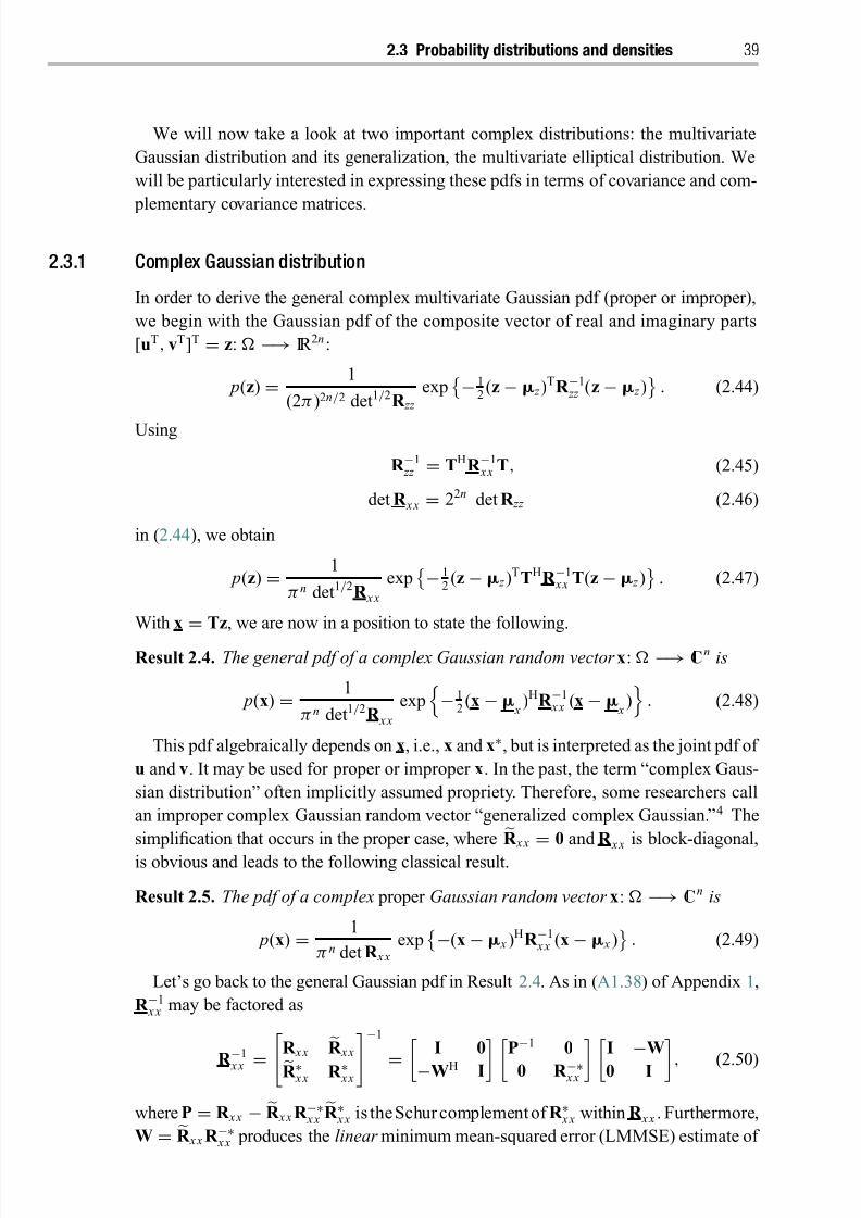
8/21/2019 Statistical Signal Processing of Complex-Valued Data.pdf
http://slidepdf.com/reader/full/statistical-signal-processing-of-complex-valued-datapdf 61/330
2.3 Probability distributions and densities 39
We will now take a look at two important complex distributions: the multivariate
Gaussian distribution and its generalization, the multivariate elliptical distribution. We
will be particularly interested in expressing these pdfs in terms of covariance and com-
plementary covariance matrices.
2.3.1 Complex Gaussian distribution
In order to derive the general complex multivariate Gaussian pdf (proper or improper),
we begin with the Gaussian pdf of the composite vector of real and imaginary parts
[uT, vT]T = z: −→ IR 2n:
p(z) = 1
(2π)2n/2 det1/2R zz
exp
− 1
2(z − z )
TR −1 zz (z − z )
. (2.44)
Using
R −1 zz = THR −1
x x T, (2.45)
det R x x = 22n det R zz (2.46)
in (2.44), we obtain
p(z) = 1
π n det1/2R x x
exp− 1
2(z − z )
TTHR −1 x x T(z − z )
. (2.47)
With x
=Tz, we are now in a position to state the following.
Result 2.4. The general pdf of a complex Gaussian random vector x: −→ Cn is
p(x) = 1
π n det1/2R x x
exp− 1
2(x −
x)HR −1
x x (x − x
)
. (2.48)
This pdf algebraically depends on x, i.e., x and x∗, but is interpreted as the joint pdf of
u and v. It may be used for proper or improper x. In the past, the term “complex Gaus-
sian distribution” often implicitly assumed propriety. Therefore, some researchers call
an improper complex Gaussian random vector “generalized complex Gaussian.”4 The
simplification that occurs in the proper case, where R x x
=0 and R x x is block-diagonal,
is obvious and leads to the following classical result.
Result 2.5. The pdf of a complex proper Gaussian random vector x: −→ Cn is
p(x) = 1
π n det R x x
exp−(x − x )HR −1
x x (x − x )
. (2.49)
Let’s go back to the general Gaussian pdf in Result 2.4. As in (A1.38) of Appendix 1,
R −1 x x may be factored as
R −1
x x = R x x R x xR ∗ x x R ∗ x x−1
= I 0
−WH I P−1 0
0 R −∗ x x I
−W
0 I , (2.50)
where P = R x x − R x x R −∗ x xR ∗ x x is theSchur complementof R ∗ x x within R x x . Furthermore,
W = R x x R −∗ x x produces the linear minimum mean-squared error (LMMSE) estimate of
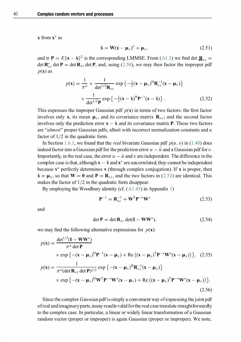
8/21/2019 Statistical Signal Processing of Complex-Valued Data.pdf
http://slidepdf.com/reader/full/statistical-signal-processing-of-complex-valued-datapdf 62/330
40 Complex random vectors and processes
x from x∗ as
x = W(x − x )∗ + x , (2.51)
and tr P = E x − x2
is the corresponding LMMSE. From (A1.3) we find det R x x =det R ∗ x x det P = det R x x det P, and, using (2.50), we may then factor the improper pdf
p(x) as
p(x) = 1
π n × 1
det1/2R x x
exp− 1
2(x − x )HR −1
x x (x − x )
× 1
det1/2Pexp
− 12(x − x)HP−1(x − x)
. (2.52)
This expresses the improper Gaussian pdf p(x) in terms of two factors: the first factor
involves only x, its mean x
, and its covariance matrix R x x
; and the second factor
involves only the prediction error x − x and its covariance matrix P. These two factors
are “almost ” proper Gaussian pdfs, albeit with incorrect normalization constants and a
factor of 1/2 in the quadratic form.
In Section 1.6.1, we found that the real bivariate Gaussian pdf p(u, v) in (1.48) does
indeed factor into a Gaussian pdf for the prediction error u − u and a Gaussian pdf for v.
Importantly, in the real case, the error u − u and v are independent. The difference in the
complex case is that, although x − x and x∗ are uncorrelated, they cannot be independent
because x∗ perfectly determines x (through complex conjugation). If x is proper, then
x
= x , so that W
=0 and P
=R x x , and the two factors in (2.52) are identical. This
makes the factor of 1/2 in the quadratic form disappear.
By employing the Woodbury identity (cf. (A1.43) in Appendix 1)
P−1 = R −1 x x + WTP−∗W∗ (2.53)
and
det P = det R x x det(I − WW∗), (2.54)
we may find the following alternative expressions for p(x):
p(x) = det1/2
(I − WW∗)π n det P
× exp−(x − x )HP−1(x − x ) + Re
(x − x )TP−∗W∗(x − x )
, (2.55)
p(x) = 1
π n(det R x x det P)1/2 exp
−(x − x )HR −1 x x (x − x )
× exp
−(x − x )HWTP−∗W∗(x − x ) + Re(x − x )TP−∗W∗(x − x )
.
(2.56)
Since the complex Gaussian pdf is simply a convenient way of expressing the joint pdf of real andimaginaryparts, many results valid for the real case translate straightforwardly
to the complex case. In particular, a linear or widely linear transformation of a Gaussian
random vector (proper or improper) is again Gaussian (proper or improper). We note,

8/21/2019 Statistical Signal Processing of Complex-Valued Data.pdf
http://slidepdf.com/reader/full/statistical-signal-processing-of-complex-valued-datapdf 63/330
2.3 Probability distributions and densities 41
however, that a widely linear transformation of a proper Gaussian will generally produce
an improper Gaussian, and a widely linear transformation of an improper Gaussian may
produce a proper Gaussian.
2.3.2 Conditional complex Gaussian distribution
If two real random vectors z = [uT, vT]T : −→ IR 2n and w = [aT, bT]T : −→ IR 2m
are jointly Gaussian, then the conditional density for z given w is Gaussian,
p(z|w) = 1
(2π)2n/2 det1/2R zz |wexp
− 12(z − z |w)TR −1
zz |w(z − z |w)
(2.57)
with conditional mean vector
z |w = z + R z wR −1ww(w − w) (2.58)
and conditional covariance matrix
R zz |w = R zz − R z wR −1ww R T z w . (2.59)
This result easily generalizes to the complex case. Let x = u + jv: −→ Cn and
y = a + jb: −→ Cm , and y = Tw. Then the augmented conditional mean vector is
x
| y
= x| y
∗ x| y = T z
|w
=T z
+(TR z wTH)(T−HR −1
ww T−1)T(w
−w)
= x + R x y R −1
yy (y − y
). (2.60)
The augmented conditional covariance matrix is
R x x| y = TR zz |wTH = TR zz TH − (TR z wTH)(T−HR −1
ww T−1)(TR T z wTH)
= R x x − R x y R −1 yy R H x y . (2.61)
Therefore, the conditional pdf takes the general form
p(x|y) = 1π n det1/2R x x| y
exp− 12 (x − x | y)HR −1
x x| y(x − x| y) . (2.62)
Using the matrix inversion lemma for R −1 x x| y , it is possible to derive an expression that
explicitly shows the dependence of p(x|y) on y and y∗. However, we shall postpone this
until our discussion of widely linear estimation in Section 5.4.
Definition 2.2. Two complex random vectors x and y are called jointly proper if the
composite vector [xT, yT]T is proper. This means they must be individually proper,
R x x = 0 and R yy = 0 , and also cross-proper, R x y = 0.
If x and y are jointly proper, the conditional Gaussian density for x given y is
p(x|y) = 1
π n det R x x | yexp
−(x − x| y)HR −1 x x| y(x − x| y)
(2.63)
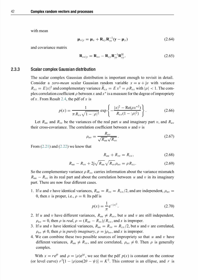
8/21/2019 Statistical Signal Processing of Complex-Valued Data.pdf
http://slidepdf.com/reader/full/statistical-signal-processing-of-complex-valued-datapdf 64/330
42 Complex random vectors and processes
with mean
x| y = x + R x y R −1 yy (y − y) (2.64)
and covariance matrix
R x x| y = R x x − R x y R −1 yy R H x y . (2.65)
2.3.3 Scalar complex Gaussian distribution
The scalar complex Gaussian distribution is important enough to revisit in detail.
Consider a zero-mean scalar Gaussian random variable x = u + jv with variance
R x x = E | x|2 and complementary variance
R x x = E x2 = ρ R x x with |ρ| < 1. The com-
plex correlation coefficient ρ between x and x∗ is a measure for the degree of impropriety
of x . From Result 2.4, the pdf of x is
p( x) = 1
π R x x
1 − |ρ|2
exp
−| x|2 − Re(ρ x∗2)
R x x (1 − |ρ|2)
. (2.66)
Let Ruu and Rvv be the variances of the real part u and imaginary part v, and Ruv
their cross-covariance. The correlation coefficient between u and v is
ρuv = Ruv√
Ruu
√ Rvv
. (2.67)
From (2.21) and (2.22) we know that
Ruu + Rvv = R x x , (2.68)
Ruu − Rvv + 2j
Ruu
Rvv ρuv = ρ R x x . (2.69)
So the complementary variance ρ R x x carries information about the variance mismatch
Ruu − Rvv in its real part and about the correlation between u and v in its imaginary
part. There are now four different cases.
1. If u and v have identical variances, Ruu = Rvv = R x x /2, and are independent, ρuv =0, then x is proper, i.e., ρ = 0. Its pdf is
p( x) = 1
πe−| x|
2
. (2.70)
2. If u and v have different variances, Ruu = Rvv , but u and v are still independent,
ρuv = 0, then ρ is real , ρ = ( Ruu − Rvv )/ R x x , and x is improper.
3. If u and v have identical variances, Ruu = Rvv = R x x /2, but u and v are correlated,
ρuv = 0, then ρ is purely imaginary, ρ = jρuv , and x is improper.
4. We can combine these two possible sources of impropriety so that u and v have
different variances, Ruu
= Rvv , and are correlated, ρuv
=0. Then ρ is generally
complex.
With x = r e jθ and ρ = |ρ|e jψ , we see that the pdf p( x) is constant on the contour
(or level curve) r 2[1 − |ρ|cos(2θ − ψ)] = K 2. This contour is an ellipse, and r is
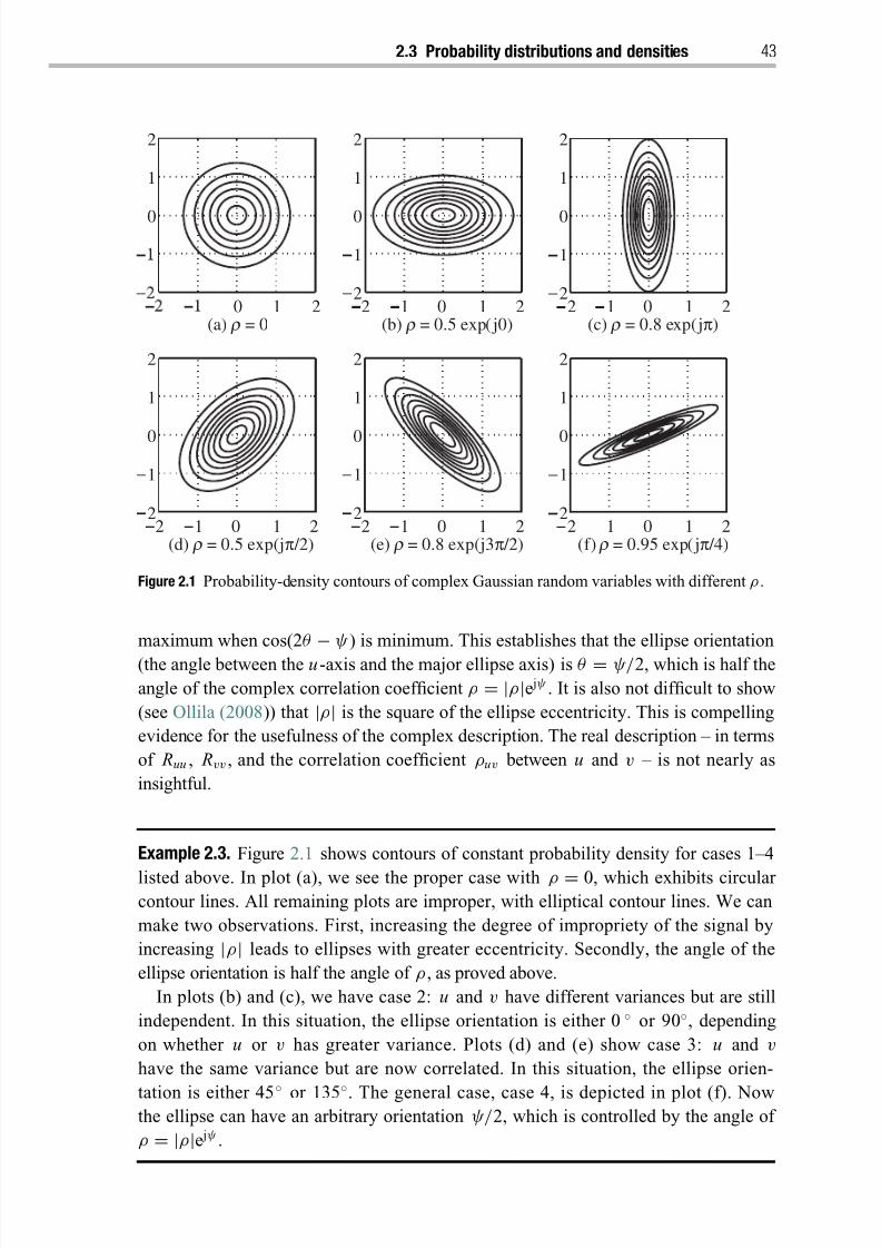
8/21/2019 Statistical Signal Processing of Complex-Valued Data.pdf
http://slidepdf.com/reader/full/statistical-signal-processing-of-complex-valued-datapdf 65/330
2.3 Probability distributions and densities 43
(a) r = 00 1 2
0
1
2
(b) r = 0.5 exp(j0)2 1 0 1 2
2
1
0
1
2
(c) r = 0.8 exp(jπ)2 1 0 1 2
2
1
0
1
2
(d) r = 0.5 exp(jπ /2)2 1 0 1 2
2
1
0
1
2
(e) r = 0.8 exp(j3π /2)2 1 0 1 2
2
1
0
1
2
(f) r = 0.95 exp(jπ /4)2 1 0 1 2
2
1
0
1
2
Figure 2.1 Probability-density contours of complex Gaussian random variables with different ρ .
maximum when cos(2θ
−ψ) is minimum. This establishes that the ellipse orientation
(the angle between the u-axis and the major ellipse axis) is θ = ψ/2, which is half the
angle of the com plex correlation coefficient ρ = |ρ|e jψ . It is also not difficult to show
(see Ollila (2008)) that |ρ| is the square of the ellipse eccentricity. This is compelling
evidence for the usefulness of the complex description. The real description – in terms
of Ruu , Rvv , and the correlation coefficient ρuv between u and v – is not nearly as
insightful.
Example 2.3. Figure 2.1 shows contours of constant probability density for cases 1–4
listed above. In plot (a), we see the proper case with ρ = 0, which exhibits circular contour lines. All remaining plots are improper, with elliptical contour lines. We can
make two observations. First, increasing the degree of impropriety of the signal by
increasing |ρ| leads to ellipses with greater eccentricity. Secondly, the angle of the
ellipse orientation is half the angle of ρ , as proved above.
In plots (b) and (c), we have case 2: u and v have different variances but are still
independent. In this situation, the ellipse orientation is either 0◦ or 90◦, depending
on whether u or v has greater variance. Plots (d) and (e) show case 3: u and v
have the same variance but are now correlated. In this situation, the ellipse orien-
tation is either 45◦ or 135◦. The general case, case 4, is depicted in plot (f). Nowthe ellipse can have an arbitrary orientation ψ/2, which is controlled by the angle of
ρ = |ρ|e jψ .
8/21/2019 Statistical Signal Processing of Complex-Valued Data.pdf
http://slidepdf.com/reader/full/statistical-signal-processing-of-complex-valued-datapdf 66/330
44 Complex random vectors and processes
With u = r cos θ , v = r sin θ , d u d v = r d r d θ , it is possible to change variables and
obtain the pdf for the polar coordinates (r , θ )
pr θ
(r , θ )=
r
π R x x 1 − |ρ|2exp−r 2[1 − |ρ| cos(2θ − ψ)]
R x x (1 − |ρ|2) , (2.71)
where x = r e jθ and ρ = |ρ|e jψ . The marginal pdf for r is obtained by integrating over
θ ,
pr (r ) = 2r
R x x
1 − |ρ|2
exp
− r 2
R x x (1 − |ρ|2)
I 0
r 2|ρ|
R x x (1 − |ρ|2)
, r > 0,
(2.72)
where I 0 is the modified Bessel function of the first kind of order 0:
I 0( z ) =1
π π
0 e
z cos θ
d θ . (2.73)
This pdf is invariant with respect to ψ . It is plotted in Fig. 1.9 in Section 1.6 for several
values of |ρ|. For ρ = 0, it is the Rayleigh pdf
pr (r ) = r
R x x /2 exp
− r 2
R x x
. (2.74)
This suggests that we call pr (r ) in (2.72) the improper Rayleigh pdf .5 Integrating
pr θ (r , θ ) over r yields the marginal pdf for θ :
pθ (θ ) = 1 − |ρ|2
2π[1 − |ρ|cos(2θ − ψ)], −π < θ ≤ π. (2.75)
This pdf is shown in Fig. 1.9 for several values of |ρ|. For ρ = 0, the pdf is uniform. For
larger |ρ|, the pdf develops two peaks at θ = ψ/2 and θ = ψ/2 − π .
If |ρ| = 1, x isa singular randomvariable because the support of the pdf p( x) collapses
to a line in the complex plane and the pdf (2.66) must be expressed using a Dirac δ-
function. This case is called maximally improper (terms used by other researchers are
rectilinear and strict-sense noncircular ). If x is maximally improper, we can express it as
x
=ae jψ/2
=a cos(ψ/2)
+ ja sin(ψ/2),where a isa real Gaussianrandomvariablewith
zero mean and variance R x x . Hence, the radius-squared r 2 of x /√ R x x is χ 2-distributed with one degree of freedom, and the angle θ takes on values ψ/2 and ψ/2 − π , each
with probability equal to 1/2.
2.3.4 Complex elliptical distribution
A generalization of the Gaussian distribution, which has found some interesting appli-
cations in communications, is the family of elliptical distributions. We could proceed as
in the Gaussian case by starting with the pdf of an elliptical distribution for a composite
real random vector z and then deriving an expression in terms of complex x. Instead,we will directly modify the improper Gaussian pdf (2.48) by replacing the exponential
function with a nonnegative function g : [0,∞) −→ [0,∞), called the pdf generator ,
that satisfies ∞
0 t n−1 g (t )d t < ∞. This necessitates two changes: First, since we do not
8/21/2019 Statistical Signal Processing of Complex-Valued Data.pdf
http://slidepdf.com/reader/full/statistical-signal-processing-of-complex-valued-datapdf 67/330
2.3 Probability distributions and densities 45
yet know the second-order moments of x, the matrix used in the expression for the pdf
may no longer be the augmented covariance matrix of x. Hence, instead of R x x , we use
the augmented generating matrix
H x x = H x x H x xH∗ x x H∗
x x
to denote an arbitrary augmented positive definite matrix of size 2n × 2n. Secondly,
we need to introduce a normalizing constant cn to ensure that p(x) is a valid pdf that
integrates to 1.
We now state the general form of the complex elliptical pdf, which is a straightforward
generalization of the real elliptical pdf, due to Ollila and Koivunen (2004).
Definition 2.3. The pdf of a complex elliptical random vector x:
−→Cn is
p(x) = cn
det1/2H x x
g
(x − x
)HH−1 x x (x −
x)
. (2.76)
The normalizing constant cn is given by
cn =(n − 1)!
π n ∞
0 t 2n−1 g (t 2)d t
. (2.77)
If the mean exists, the parameter x in the pdf (2.76) is the augmented mean of x. This
indicates that the mean is independent of the choice of pdf generator. However, there
are distributions for which some or all moments are undefined. For instance, none of the moments exist for the Cauchy distribution, which belongs to the family of elliptical
distributions. In this case, x should be treated simply as a parameter of the pdf but not
its augmented mean.
Since the complex elliptical pdf (2.76) contains the same quadratic form as the
complex Gaussian pdf (2.48), we can obtain straightforward analogs of (2.55) and
(2.56), which are expressions in terms of x and x∗. We can also write down the expres-
sion for the pdf of an elliptical random vector with zero complementary generating
matrix.
Result 2.6. The pdf of a complex elliptical random vector x: −→ Cn with H x x = 0is
p(x) = cn
det H x x
g
2(x − x )HH−1 x x (x − x )
, (2.78)
with normalizing constant cn given by ( 2.77 ).
A good overview of real and complex elliptical distributions is given by Fang et al .
(1990). However, Fang et al. consider only complex elliptical distributions with zero
complementary generating matrix. Thus, Ollila and Koivunen (2004) refer to the gen-
eral complex elliptical pdf in Definition 2.3 as a “generalized complex elliptical” pdf.
The family of complex elliptical distributions contains some important subclasses of
distributions.

8/21/2019 Statistical Signal Processing of Complex-Valued Data.pdf
http://slidepdf.com/reader/full/statistical-signal-processing-of-complex-valued-datapdf 68/330
46 Complex random vectors and processes
(a) r = 00 1 2
0
1
2
(b) r = 0.5 exp(jπ /2)2 1 0 1 2
2
1
0
1
2
(c) r = 0.95 exp( jπ /4)2 1 0 1 2
2
1
0
1
2
Figure 2.2 Probability-density contours of complex Cauchy random variables with different ρ .
The complex multivariate Gaussian distribution, for pdf generator g (t ) = exp(−t /2). The complex multivariate t -distribution, with pdf given by
p(x) = 2n (n + k /2)
(π k )n(k /2)det1/2H x x
1 + k −1(x −
x)HH−1
x x (x − x
)−n−k /2
, (2.79)
where k is an integer. We note that the Gamma function satisfies (n) = (n − 1)! if n
is a positive integer. The complex multivariate Cauchy distribution, which is a special case of the complex
multivariate t -distribution with k = 1. Its pdf is
p(x) = 2n (n + 1/2)
π n+1/2 det1/2H x x 1 + (x −
x)HH−1
x x (x − x
)
−n−1/2
. (2.80)
None of the moments of the Cauchy distribution exist.
Example 2.4. Similarly to Example 2.3, consider a scalar complex Cauchy pdf with
µ x = 0 (which is the median but not the mean, since the mean does not exist) and
augmented generator matrix
H x x =
1 ρ
ρ∗ 1
, |ρ| < 1. (2.81)
Its pdf is
p( x) = 1
π
1 − |ρ|2
1 + | x|2 − Re(ρ x∗2)
1 − |ρ|2−3/2
. (2.82)
If ρ = 0, then the pdf is p( x) = (1/π )(1 + | x|2)−3/2.
Just as for the scalar complex Gaussian pdf, the scalar complex Cauchy pdf is constant
on elliptical contours whose major axis is ψ/2, half the angle of ρ = |ρ|e jψ . Figure 2.2
shows contours of constant probability density for three Cauchy random variables. Plots
(a), (b), and (c) in this figure should be compared with plots (a), (d), and (f) in Fig. 2.1,
respectively, for the Gaussian case. The main difference is that Cauchy random variables
have much heavier tails than Gaussian random variables. From the expression (2.82), itis straightforward to write down the joint pdf in polar coordinates (r , θ ), and not quite
as straightforward to integrate with respect to r or θ to obtain the marginal pdfs.
8/21/2019 Statistical Signal Processing of Complex-Valued Data.pdf
http://slidepdf.com/reader/full/statistical-signal-processing-of-complex-valued-datapdf 69/330
2.4 ML covariance estimators: Wishart distribution 47
Complex elliptical distributions have a number of desirable properties.
The mean of x (if it exists) is independent of the choice of pdf generator g . The augmented covariance matrix of x (if it exists) is proportional to the augmented
generating matrix H x x . The proportionality factor depends on g , and is most eas-
ily determined using the characteristic function of x. Therefore, if the second-order
moments exist, the pdf (2.76) is the pdf of a complex improper elliptical random
vector, and the pdf (2.78) for H x x = 0 is the pdf of a complex proper elliptical random
vector with R x x = 0. This is due to Result 2.8, to be discussed in Section 2.5. All marginal distributions are also elliptical. If y: −→ Cm contains components of
x: −→ Cn , m < n , then y is elliptical with the same g as x, and y contains the
corresponding components of x . The augmented generating matrix of y, H yy , is the
sub-matrix of H x x that corresponds to the components that y extracts from x. Let y = M x + b, where M is a given 2m × 2n augmented matrix and b is a given
2m × 1 augmented vector. Then y is elliptical with thesame g as x and y = M
x + b
and H yy = M H x x MH. If x: −→ Cn and y: −→ Cm are jointly elliptically distributed with pdf generator
g , then the conditional distribution of x given y is also elliptical with
x| y =
x + H x y H−1
yy (y − y
), (2.83)
which is analogous to the Gaussian case (2.60), and augmented conditional generating
matrix
H x x| y = H x x − H x y H−1 yy HH
x y , (2.84)
which is analogous to the Gaussian case (2.61). However, the conditional distribution
will in general have a different pdf generator than x and y.
2.4 Sufficient statistics and ML estimators for covariances:
complex Wishart distribution
Let’s draw a sequence of M independent and identically distributed (i.i.d.) samples
{xi } M i=1 from a complex multivariate Gaussian distribution with mean x and augmented
covariance matrix R x x . We assemble these samples in a matrix X = [x1, x2, . . . , x M ],
and let X = [x1, x2, . . . , x M ] denote the augmented sample matrix. Using the expression
for the Gaussian pdf in Result 2.4, the joint pdf of the samples {xi } M i=1 is
p(X)=
π− Mn (det R x x
)− M /2 exp−1
2
M
m=1
(xm −
x
)HR −1
x x (x
m −
x) (2.85)
= π− Mn (det R x x )− M /2 exp
− M
2 tr(R −1
x x S x x )
. (2.86)
8/21/2019 Statistical Signal Processing of Complex-Valued Data.pdf
http://slidepdf.com/reader/full/statistical-signal-processing-of-complex-valued-datapdf 70/330
48 Complex random vectors and processes
In this expression, S x x is the augmented sample covariance matrix
S x x = S x x
S x x
S∗ x x
S∗ x x =
1
M
M
m=1
(xm − m x )(xm − m x )H = 1
M X XH − m x mH
x (2.87)
and m x is the augmented sample mean vector
m x =1
M
M m=1
xm . (2.88)
The augmented sample covariance matrix contains the sample Hermitian covariance
matrix
S x x =1
M
M
m=1
(xm − m x )(xm − m x )H
=1
M XXH
− m x mH
x (2.89)
and the sample complementary covariance matrix
S x x =1
M
M m=1
(xm − m x )(xm − m x )T = 1
M XXT − m x mT
x . (2.90)
We now appeal to the Fisher–Neyman factorization theorem to argue that m x and S x x
are a pair of sufficient statistics for x
and R x x , or, equivalently, (m x , S x x ,
S x x ) are a
set of sufficient statistics for ( x , R x x , R x x ).
It is a straightforward consequence of the corresponding result for the real case that the
sample mean m x is also a maximum-likelihood estimator of the mean x , and the sample
covariances (S x x ,S x x )are maximum-likelihood estimatorsof thecovariances (R x x , R x x ).
Note that the sample mean is independent of the sample covariance matrices, but the
Hermitian and complementary sample covariances are not independent.
Complex Wishart distribution
How are the sample covariance matrices distributed? Let ui and vi be the real and
imaginaryparts of the samplevector xi
=ui
+ jvi ,and U and V be the real and imaginary
parts of the sample matrix X = U + jV. Moreover, let Z = [UT, VT]T. If the samples xi
are drawn from a zero-mean Gaussian distribution, then W zz = ZZT = M S zz is Wishart
distributed :
pW zz (W zz ) =
[det W zz ]( M −1)/2−n exp
− 12 tr(R −1
zz W zz )
2 Mn 2n( M /2)[det R zz ] M /2 . (2.91)
In this expression, 2n( M /2) is the multivariate Gamma function
2n( M /2) = π
n(2n
−1)/2
2n
i=1
[( M − i + 1)/2]. (2.92)
By following a path similar to the derivation of the complex Gaussian pdf in Section
2.3.1, it is possible to rewrite the pdf of real W zz in terms of the complex augmented
8/21/2019 Statistical Signal Processing of Complex-Valued Data.pdf
http://slidepdf.com/reader/full/statistical-signal-processing-of-complex-valued-datapdf 71/330
2.5 Characteristic function 49
matrix W x x = TW zz TH = X XH = M S x x and the augmented covariance matrix R x x as
pW zz (W x x ,
W x x ) = [det W x x ]( M −1)/2−n exp
− 12 tr(R −1
x x W x x )
2n( M −2n−1)2n( M /2)[det R x x ] M /2 . (2.93)
If x is proper , then R x x = 0 and R x x = Diag(R x x , R ∗ x x ). However, this does not imply
that the sample complementary covariance matrix vanishes. In general, W x x = XXT =0. Thus, for proper x the pdf (2.93) simplifies, but it is still the pdf of real W zz , expressed
as a function of both W x x = XXH and W x x = XXT:
pW zz (W x x , W x x )= [det W x x det(W∗
x x − W∗ x x W−1
x xW x x )]( M −1)/2−n exp
− tr(R −1 x x W x x )
2n( M −2n−1)2n( M /2)[det R x x ] M
.
(2.94)
In order to obtain the marginal pdf of W x x , we would need to integrate pW zz (W x x , W x x )for given W x x over all W∗
x x − W∗ x x W−1
x xW x x > 0. Alternatively, we can compute the
characteristic function of W zz , set all complementary terms equal to zero, and then
compute the corresponding pdf of W x x . The last of these three steps is the tricky one.
In essence, this is the approach followed by Goodman (1963), who showed that
p(W x x ) = [det W x x ] M −n exp−tr(R −1
x x W x x )
cn( M )[det R x x ] M
, (2.95)
where cn( M ) is
cn( M ) = π n(n−1)/2 n
i=1
( M − i)! (2.96)
The marginal pdf p(W x x ) for proper x in (2.95) is what is commonly referred to as the
complex Wishart distribution. Its support is W x x > 0, and it is interpreted as the joint
pdf of real and imaginary parts of W x x .
An alternative, simpler, derivation of the complex Wishart distribution, not based
on the characteristic function, was given by Srivastava (1965). The derivation of the
marginal pdf p(W x x ) for improper x is an unresolved problem.
2.5 Characteristic function and higher-order statistical description
The characteristic function is a characterization equivalent to the pdf of a random vector,
yet working with the characteristic function can be more convenient. For the composite
real random vector z = [uT, vT]T, the characteristic function is defined in terms of
su ∈ IR n and sv ∈ IR n (which are not random) as
ψ(su , sv) = E exp j(sTu u + sT
v v) . (2.97)
This is the inverse Fourier transform of the pdf p(u, v). If we let x = u + jv (random)
and s = su + jsv (not random), we have
sTu u + sT
v v = 12
sHx = Re(sHx). (2.98)
8/21/2019 Statistical Signal Processing of Complex-Valued Data.pdf
http://slidepdf.com/reader/full/statistical-signal-processing-of-complex-valued-datapdf 72/330
50 Complex random vectors and processes
Thus, we may define the characteristic function of x as
ψ(s) = E
exp
j
2sHx
= E
exp[j Re(sHx)]
. (2.99)
2.5.1 Characteristic functions of Gaussian and elliptical distributions
The characteristic function of a real elliptical random vector z (cf. Fang et al . (1990)) is
ψ(su , sv) = exp(j
sTu sT
v
z )φ
sT
u sTv
R zz
su
sv
, (2.100)
where φ is a scalar function that determines the distribution. From this we obtain the
following result, which was first published by Ollila and Koivunen (2004).
Result 2.7. The characteristic function of a complex elliptical random vector x is
ψ(s) = exp
j
2sH
x
φ
14
sHH x x s
= exp[j Re(sH x )]φ
12
sHH x x s + 12 Re(sHH x x s∗)
. (2.101)
If x is complex Gaussian, then H x x = R x x , H x x = R x x , and φ(t ) = exp(−t /2).
Both expressions in (2.101) – in terms of augmented vectors and in terms of un-
augmented vectors – are useful. It is easy to see the simplification that occurs whenH x x = 0 or R x x = 0, as when x is a proper Gaussian random vector.The characteristic function has a number of useful properties. It exists even when
the augmented covariance matrix R x x (or the covariance matrix R x x ) is singular, a
property not shared by the pdf. The characteristic function also allows us to state a
simple connection between R x x and H x x for elliptical random vectors (consult Fang
et al . (1990) for the expression in the real case).
Result 2.8. Let x be a complex elliptical random vector with characteristic function
( 2.101 ). If the second-order moments of x exist, then
R x x = cH x x with c = −2 d d t
φ(t )|t =0. (2.102)
It follows that R x x = cH x x and R x x = cH x x . In particular, we see that x is proper
if and only if H x x = 0. For Gaussian x, φ(t ) = exp(−t /2) and therefore c = 1, as
expected.
2.5.2 Higher-order moments
First- andsecond-order moments suffice for thecharacterization of many probabilitydis-
tributions. They also suffice for the solution of mean-squared-error estimation problemsand Gaussian detection problems. Nevertheless, higher-order moments and cumulants
carry important information that can be exploited when the underlying probability distri-
bution is unknown. For a complexrandomvariable x , there are N + 1 different N th-order
8/21/2019 Statistical Signal Processing of Complex-Valued Data.pdf
http://slidepdf.com/reader/full/statistical-signal-processing-of-complex-valued-datapdf 73/330
2.5 Characteristic function 51
moments E ( x q x∗ N −q ), with q = 0, 1, 2, . . . , N . It is immediately clear that there can
be only a maximum of N /2 + 1 distinct moments, where · denotes the floor func-
tion. Since E ( x q x∗ N −q) = [ E ( x N −q x∗q )]∗ we can restrict q to q = 0, 1, 2, . . . , N /2.
Because moments become increasingly difficult to estimate in practice for larger N , itis rare to consider moments with N > 4.
Summarizing all N th-order moments for a complex random vector x requires the use
of tensor algebra, as developed in the complex case by Amblard et al . (1996a). We will
avoid this by considering only moments of individual components of x. These are of the
form E ( x1
i1 x2
i2· · · x N
i N ), where 1 ≤ i j ≤ n, j = 1, . . . , N , and j indicates whether or
not x i j is conjugated. Again, there are only a maximum of N /2 + 1 distinct moments
since E ( x1
i1 x2
i2· · · x N
i N ) = [ E (( x
1
i1)∗( x
2
i2)∗ · · · ( x N
i N )∗)]∗.
As in the real case, the moments of x can be calculated from the characteristic
function. To this end, we use two generalized complex differential operators for complex
s = su + j sv , which are defined as
∂
∂ s
1
2
∂
∂ su
− j ∂
∂ sv
, (2.103)
∂
∂ s∗
1
2
∂
∂ su
+ j ∂
∂ sv
(2.104)
and discussed in Appendix 2. From the complex Taylor-series expansion of ψ(s), we
can obtain the N th-order moment from the characteristic function. The following result
is due to Amblard et al . (1996a).
Result 2.9. For a random vector x with characteristic function ψ(s) , the N th-order
moment can be computed as
E ( x1
i1 x2
i2· · · x N
i N ) = 2 N
j N
∂ N ψ(s)
(∂ s1
i1)∗(∂ s
2
i2)∗ · · · (∂ s
N
i N )∗
s=0
. (2.105)
Example 2.5. Consider a scalar Gaussian random variable with zero mean, variance R x x ,
and complementary variance
R x x = ρ R x x , whose pdf is
p( x) = 1
π R x x
1 − |ρ|2
exp−| x|2 − Re(ρ x∗2)
R x x (1 − |ρ|2)
. (2.106)
Its characteristic function is
ψ( s) = exp− 1
4 R x x [| s|2 + Re(ρ s∗2)]
. (2.107)
The pdf p( x) is not defined for |ρ| = 1 because the support of the pdf collapses to a line
in the complex plane. The characteristic function, on the other hand, is defined for all
|ρ| ≤ 1.
Using the differentiation rules from Appendix 2, we compute the first-order partialderivative
∂ψ( s)
∂ s∗ = − 1
4 R x x ψ( s)( s + ρ s∗) (2.108)
8/21/2019 Statistical Signal Processing of Complex-Valued Data.pdf
http://slidepdf.com/reader/full/statistical-signal-processing-of-complex-valued-datapdf 74/330
52 Complex random vectors and processes
and the second-order partial derivatives
∂2ψ( s)
∂ s ∂ s∗ = − 1
4 R x x
∂ψ( s)
∂ s( s + ρ s∗) + ψ( s)
, (2.109)
∂2ψ( s)
(∂ s∗)2 = − 1
4 R x x
∂ψ( s)
∂ s∗ ( s + ρ s∗) + ρψ( s)
. (2.110)
According to Result 2.9, the variance is obtained as
E ( x∗ x) = 22
j2∂2ψ( s)
∂ s ∂ s∗
s=0
= R x x (2.111)
and the complementary variance as
E ( x x) =22
j2∂2ψ( s)
(∂ s∗)2 s=0
= ρ R x x . (2.112)
2.5.3 Cumulant-generating function
The cumulant-generating function of x is defined as
(s) = log ψ(s) = log E
exp
j Re(sHx)
. (2.113)
The cumulants are found from the cumulant-generating function just like the momentsare from the characteristic function:
Cum( x1
i1 x2
i2· · · x N
i N ) = 2 N
j N
∂ N (s)
(∂ s1
i1)∗(∂ s
2
i2)∗ · · · (∂ s
N
i N )∗
s=0
. (2.114)
The first-order cumulant is the mean,
Cum xi = E xi . (2.115)
For a zero-mean random vector x, the cumulants of second, third, and fourth order are
related to moments through
Cum( x1
i1 x2
i2) = E ( x
1
i1 x2
i2), (2.116)
Cum( x1
i1 x2
i2 x3
i3) = E ( x1
i1 x2
i2 x3
i3), (2.117)
Cum( x1
i1 x2
i2 x3
i3 x4
i4) = E ( x
1
i1 x2
i2 x3
i3 x4
i4) − E ( x
1
i1 x2
i2) E ( x
3
i3 x4
i4)
− E ( x1
i1 x3
i3) E ( x
2
i2 x4
i4) − E ( x
1
i1 x4
i4) E ( x
2
i2 x3
i3). (2.118)
Thus, thesecond-order cumulant is thecovariance or complementary covariance. Cumu-
lants are sometimes preferred over moments because cumulants are additive for inde- pendent random variables. For Gaussian random vectors, all cumulants of order higher
than two are zero. This leads to the following result for proper Gaussians, which is based
on (2.118) and vanishing complementary covariance terms.

8/21/2019 Statistical Signal Processing of Complex-Valued Data.pdf
http://slidepdf.com/reader/full/statistical-signal-processing-of-complex-valued-datapdf 75/330
2.5 Characteristic function 53
Result 2.10. For a proper complex Gaussian random vector x , only fourth-order
moments with two conjugated and two nonconjugated terms are nonzero. Without loss
of generality, assume that xi3 and xi4
are the conjugated terms. We then have
E ( xi1 xi2 x∗i3 x∗i4) = E ( xi1 x∗
i3) E ( xi2 x∗i4) + E ( xi1 x∗i4) E ( xi2 x∗i3). (2.119)
2.5.4 Circularity
It is also possible to define a stronger version of propriety in terms of the probability
distribution of a random vector. A vector is called circular if its probability distribution
is rotationally invariant .
Definition 2.4. A random vector x is called circular if x and x = e jαx have the same
probability distribution for any given real α.
Therefore, x must have zero mean in order to be circular. But circularity does not imply
any condition on the standard covariance matrix R x x because
R x x = E (xxH) = E (e jαxxHe− jα) = R x x . (2.120)
On the other hand,
R x x = E (xxT) = E (e jαxxTe jα) = e j2α
R x x (2.121)
can be true for arbitrary α only if R x x
=0. Because the Gaussian pdf is completely
determined by x , R x x , and R x x , we obtain the following result, due to Grettenberg
(1965).
Result 2.11. A complex zero-mean Gaussian random vector x is proper if and only if it
is circular.
This result generalizes nicely to the elliptical pdf.
Result 2.12. A complex elliptical random vector x is circular if and only if x = 0 and
the complementary generating matrix H x x = 0. If the first- and second-order moments
exist, then we may equivalently say that x is circular if and only if it has zero mean and is proper.
The first half of this result is easily obtained by inspecting the elliptical pdf, and the
second half is due to Result 2.8.
Propriety requires that second-order moments be rotationally invariant, whereas circu-
larity requires that the pdf, and thus all moments (if they exist), be rotationally invariant.
Therefore, circularity implies propriety, but not vice versa, and impropriety implies
noncircularity, but not vice versa. By extending the reasoning of (2.120) and (2.121) to
higher-order moments, we see that the following result holds.
Result 2.13. If x is circular, an Nth-order moment E ( x1
i1 x2
i2· · · x N
i N ) can be nonzero
only if it has the same number of conjugated and nonconjugated terms. In particular, all
odd moments must be zero. This holds for arbitrary N.
8/21/2019 Statistical Signal Processing of Complex-Valued Data.pdf
http://slidepdf.com/reader/full/statistical-signal-processing-of-complex-valued-datapdf 76/330
54 Complex random vectors and processes
We havealready seen a forerunner of this fact inResult 2.10. We may also be interested
in a term for a random vector that satisfies this condition up to some order N only.
Definition 2.5. A vector x is called N th-order circular or N th-order proper if the only
nonzero moments up to order N have the same number of conjugated and nonconjugated
terms. In particular, all odd moments up to order N must be zero.
Therefore, the terms proper and second-order circular are equivalent. We note that,
while this terminology is most common, there is not uniform agreement in the literature.
Some researchers use the terms “proper” and “circular” interchangeably. It is also
possible to define stronger versions of circularity, as Picinbono (1994) has done.
Do circular random vectors have spherical pdf contours?
It is instructive to first take a closer look at a scalar circular random variable x = Ae jφ .If x and e jα x have the same probability distribution, then the phase φ of x must be
uniformly distributed over [0, 2π) and independent of the amplitude A, which may have
an arbitrary distribution. This means that the pdf of x is complex elliptical with variance
R x x and zero complementary generator,
p( x) = c1
R x x
g
2| x |2 R x x
, (2.122)
as developed in Section 2.3.4. The pdf (2.122) has circular contour lines of constant
probability density. Does this result generalize to circular random vectors?
Unfortunately, nothing can be said in general about the contours of a circular random
vector x – not even that they are elliptical. Elliptical random vectors have elliptical
contours but circularity is not sufficient to make them spherical. In order to obtain
spherical contours, x must be spherically distributed , which means that x is elliptical
with x = 0 and augmented generating matrix H x x = k I for some positive constant k .
Hence, only spherical circular random vectors indeed have spherical contours.
2.6 Complex random processes
In this section, we extend some of the ideas introduced so far to a continuous-time
complex random process x(t ) = u(t ) + jv(t ), which is built from two real-valued ran-
dom processes u(t ) and v(t ) defined on IR. We restrict our attention to a second-order
description of wide-sense stationary processes. Higher-order statistical characterizations
and concepts such as circularity of random processes are more difficult to treat than in
the vector case, and we postpone a discussion of more advanced topics to Chapters 8
and 9.6
To simplify notation in this section, we will assume that x(t ) has zero mean. Thecovariance function of x (t ) is denoted by
r x x (t , τ ) = E [ x(t + τ ) x∗(t )], (2.123)
8/21/2019 Statistical Signal Processing of Complex-Valued Data.pdf
http://slidepdf.com/reader/full/statistical-signal-processing-of-complex-valued-datapdf 77/330
2.6 Complex random processes 55
and the complementary covariance function of x (t ) is
r x x (t , τ ) = E [ x(t + τ ) x(t )]. (2.124)
We also introduce the augmented signal x(t ) = x(t ) x∗(t )T
, whosecovariance matrix
R x x (t , τ ) = E [x(t + τ )xH(t )] =
r x x (t , τ ) r x x (t , τ )
r ∗ x x (t , τ ) r ∗ x x (t , τ )
(2.125)
is called the augmented covariance function of x (t ).
2.6.1 Wide-sense stationary processes
Definition 2.6. A signal x(t ) is wide-sense stationary (WSS) if and only if R x x (t , τ ) is
independent of t. That is, both the covariance function r x x (t , τ ) and the complementarycovariance function r x x (t , τ ) are independent of t.
This definition, in keeping with our general philosophy outlined in Section 2.2.1, calls
x(t ) WSS ifand only if its real and imaginary parts u(t )and v(t ) are jointly WSS. We note
that some researchers call a complex signal x(t ) WSS if r x x (t , τ ) alone is independent
of t , and second-order stationary if both r x x (t , τ ) and r x x (t , τ ) are independent of t . If
x(t ) is WSS, we drop the t -argument from the covariance functions. The covariance and
complementary covariance functions then have the symmetries
r x x (τ ) = r ∗ x x (−τ ) and r x x (τ ) = r x x (−τ ). (2.126)
The Fourier transform of R x x (τ ) is the augmented power spectral density (PSD) matrix
P x x ( f ) =
P x x ( f ) P x x ( f ) P ∗ x x (− f ) P ∗ x x (− f )
. (2.127)
The augmented PSD matrix contains the PSD P x x ( f ), which is the Fourier transform
of r x x (τ ), and the complementary power spectral density (C-PSD)
P x x ( f ), which is the
Fourier transform of r x x (τ ). The augmented PSD matrix is positive semidefinite, which
implies the following result.
Result 2.14. There exists a WSS random process x(t ) with PSD P x x ( f ) and C-PSD P x x ( f ) if and only if
(1) the PSD is real and nonnegative (but not necessarily even),
P x x ( f ) ≥ 0; (2.128)
(2) the C-PSD is even (but generally complex),
P x x
( f )= P
x x(−
f ); (2.129)
(3) the PSD provides a bound on the magnitude of the C-PSD,
| P x x ( f )|2 ≤ P x x ( f ) P x x (− f ). (2.130)

8/21/2019 Statistical Signal Processing of Complex-Valued Data.pdf
http://slidepdf.com/reader/full/statistical-signal-processing-of-complex-valued-datapdf 78/330
56 Complex random vectors and processes
Condition (3) is due to det P x x ( f ) ≥ 0. The three conditions in this result correspond
to the three conditions in Result 2.1 for a complex vector x. Because of (2.128) and
(2.129) the augmented PSD matrix simplifies to
P x x ( f ) = P x x ( f ) P x x ( f ) P ∗ x x ( f ) P x x (− f )
. (2.131)
The time-invariant power of x (t ) is
P x = r x x (0) = ∞−∞
P x x ( f )d f , (2.132)
regardless of whether or not x (t ) is proper.
We now connect the complex description of x (t ) = u(t ) + jv(t ) to the description in
terms of its real and imaginary parts u(t ) and v(t ). Let r uv(τ ) = E [ u(t + τ )v(t )] denotethe cross-covariance function between u(t ) and v(t ), and P uv( f ) the Fourier transform of
r uv(τ ), which is the cross-PSD between u(t ) and v(t ). Analogously to (2.20) for n = 1,
there is the connection
P x x ( f ) = T
P uu ( f ) P uv( f )
P ∗uv( f ) P vv ( f )
TH. (2.133)
From it, we find that
P x x ( f )
= P uu ( f )
+ P vv ( f )
+2 Im P uv( f ), (2.134) P x x ( f ) = P uu ( f )− P vv ( f )+ 2j Re P uv( f ), (2.135)
which are the analogs of (2.21) and (2.22). Note that, unlike the PSD of x (t ), the PSDs
of u(t ) and v(t ) are even: P uu ( f ) = P uu (− f ) and P vv ( f ) = P vv (− f ). Propriety is now
defined as the obvious extension from vectors to processes.
Definition 2.7. A complex WSS random process x(t ) is called proper if r x x (τ ) = 0 for
all τ or, equivalently,
P x x ( f ) = 0 for all f .
Equivalent conditions on real and imaginary parts for propriety are
r uu (τ ) = r vv (τ ) and r uv(τ ) = −r uv(−τ ) for all τ (2.136)
or
P uu ( f ) = P vv ( f ) and Re P uv( f ) = 0 for all f . (2.137)
Therefore, if WSS x (t ) is proper, its PSD is
P x x ( f ) = 2[ P uu ( f )− j P uv( f )] = 2[ P vv ( f )+ j P vu( f )]. (2.138)
The PSD of a proper x(t ) is even if and only if P uv( f ) = 0 because P uv( f ) is purelyimaginary and odd.
From(2.130), we obtain the following importantresult for WSSanalytic signals, which
have P x x ( f ) = 0 for f < 0, and WSS anti-analytic signals, which have P x x ( f ) = 0 for
f > 0.
8/21/2019 Statistical Signal Processing of Complex-Valued Data.pdf
http://slidepdf.com/reader/full/statistical-signal-processing-of-complex-valued-datapdf 79/330
Notes 57
Result 2.15. A WSS analytic (or anti-analytic) signal without a DC component, i.e.,
P x x (0) = 0 , is proper.
Because the equivalent complex baseband signal of a real bandpass signal is a down-
modulated analytic signal, and modulation keeps propriety intact, we also have thefollowing result.
Result 2.16. The equivalent complex baseband signal of a WSS real bandpass signal is
proper.
2.6.2 Widely linear shift-invariant filtering
Widely linear (linear–conjugate-linear) shift-invariant filtering is described in the time
domain as
y(t ) = ∞−∞
[h1(t − τ ) x(τ ) + h2(t − τ ) x∗(τ )]d τ. (2.139)
There is a slight complication with a corresponding frequency-domain expression: as
we will discuss in Section 8.1, the Fourier transform of a WSS random process x (t ) does
not exist. The way to deal with WSS processes in the frequency domain is to utilize the
Cramer spectral representation for x (t ) and y(t ),
x(t ) = ∞−∞
d ξ ( f )e j2π f t , (2.140)
y(t ) = ∞−∞
d υ( f )e j2π f t , (2.141)
where ξ ( f ) and υ( f ) are spectral processes with orthogonal increments d ξ ( f ) and
d υ( f ), respectively. This will be discussed in detail in Section 8.1. For now, we content
ourselves with stating that
d υ( f ) = H 1( f )d ξ ( f )+ H 2( f )d ξ ∗(− f ), (2.142)
which may be written in augmented notation as
d υ( f )d υ∗(− f ) = H 1( f ) H 2( f ) H ∗2 (− f ) H ∗1 (− f ) H( f )
d ξ ( f )d ξ ∗(− f ). (2.143)
The relationship between the PSDs of x (t ) and y(t ) is
P yy ( f ) = H( f )P x x ( f )HH( f ). (2.144)
Strictly linear filters have h2(t ) = 0 for all t or, equivalently, H 2( f ) = 0 for all f . It
is clear that propriety is preserved under linear filtering, and it is also preserved under
modulation.
Notes
1 The first account of widely linear filtering for complex signals seems to have been that by Brown
and Crane (1969), who used the term “conjugate linear filtering.” Gardner and his co-authors
8/21/2019 Statistical Signal Processing of Complex-Valued Data.pdf
http://slidepdf.com/reader/full/statistical-signal-processing-of-complex-valued-datapdf 80/330
58 Complex random vectors and processes
have made extensive use of widely linear filtering in the context of cyclostationary signals, in
particular for communications. See, for instance, Gardner (1993). The term “widely linear”
was introduced by Picinbono and Chevalier (1995), who presented the widely linear minimum
mean-squared error (WLMMSE) estimator for complex random vectors. Schreier and Scharf
(2003a) revisited the WLMMSE problem using the augmented complex matrix algebra.2 The terms “proper” and “pseudo-covariance” (for complementary covariance) were coined by
Neeser and Massey (1993), who looked at applications of proper random vectors in commu-
nications and information theory. The term “complementary covariance” is used by Lee and
Messerschmitt (1994), “relation matrix” by Picinbono and Bondon (1997), and “conjugate
covariance” by Gardner. Both van den Bos (1995) and Picinbono (1996) utilize what we have
called the augmented covariance matrix.
3 Conditions 1–3 in Result 2.1 for the nonsingular case were proved by Picinbono (1996). A
rather technical proof of conditions 3a and 3b was presented by Wahlberg and Schreier (2008).
4 The complex proper multivariate Gaussian distribution was introduced by Wooding (1956).
Goodman (1963) provided a more in-depth study, and also derived the proper complex Wishart
distribution. The assumption of propriety when studying Gaussian random vectors was com-monplace until van den Bos (1995) introduced the improper multivariate Gaussian distribution,
which he called “generalized complex normal.” Picinbono (1996) explicitly connected this
distribution with the Hermitian and complementary covariance matrices.
5 There are other distributions thrown off by the scalar improper complex Gaussian pdf. For
example, the conditional distribution P θ |r (θ |r ) = pr θ (r , θ )/ P r (r ), with pr θ (r , θ ) given by (2.71)
and pr (r ) by (2.72) is the von Mises distribution. The distribution of the radius-squared r 2 could
be called the improper χ 2-distribution with one degree of freedom, and the sum of the radii-
squared of k independent improper Gaussian random variables could be called the improper
χ 2-distribution with k degrees of freedom. One could also derive improper extensions of the β -
and exponential distributions.
6 Section 2.6 builds on results by Picinbono and Bondon (1997), who discussed second-order
properties of complex signals, both stationary and nonstationary, and Amblard et al . (1996b),
who developed higher-order properties of complex stationary signals. Rubin-Delanchy and
Walden (2007) present an algorithm for the simulation of improper WSS processes having
specified covariance and complementary covariance functions.

8/21/2019 Statistical Signal Processing of Complex-Valued Data.pdf
http://slidepdf.com/reader/full/statistical-signal-processing-of-complex-valued-datapdf 81/330
Part II
Complex random vectors

8/21/2019 Statistical Signal Processing of Complex-Valued Data.pdf
http://slidepdf.com/reader/full/statistical-signal-processing-of-complex-valued-datapdf 82/330
8/21/2019 Statistical Signal Processing of Complex-Valued Data.pdf
http://slidepdf.com/reader/full/statistical-signal-processing-of-complex-valued-datapdf 83/330
3 Second-order description of complexrandom vectors
In this chapter, we discuss in detail the second-order description of a complex random
vector x. We have seen in Chapter 2 that the second-order averages of x are completely
described by the augmented covariance matrix R x x . We shall now be interested in those
second-order properties of x that are invariant under two types of transformations:
widely unitary and nonsingular strictly linear.
The eigenvalues of the augmented covariance matrix R x x constitute a maximal invari-
ant for R x x under widely unitary transformation. Hence, any function of R x x that is
invariant under widely unitary transformation must be a function of these eigenvalues
only. In Section 3.1, we consider the augmented eigenvalue decomposition (EVD) of R x x
for a complex random vector x. Since we are working with an augmented matrix algebra,
this EVD looks somewhat different from what one might expect. In fact, because all
factors in the EVD must be augmented matrices, widely unitary diagonalization of R x x
is generally not possible. As an application for the augmented EVD, we discuss rank
reduction and transform coding.
In Section 3.2, we introduce the canonical correlations between x and x∗, which have
been called the circularity coefficients. These constitute a maximal invariant for R x x
under nonsingular strictly linear transformation. They are interesting and useful for a
number of reasons.
They determine the loss in entropy that an improper Gaussian random vector incurs
compared with its proper version (see Section 3.2.1).
They enable an easy characterization of the set of complementary covariance matricesfor a fixed covariance matrix (Section 3.2.3) and can be used to quantify the degree of
impropriety (Section 3.3). They define the test statistic in a generalized likelihood-ratio test for impropriety
(Section 3.4). They play a key role in blind source separation of complex signals using independent
component analysis (Section 3.5).
The connection between the circularity coefficients and the eigenvalues of R x x is
explored in Section 3.3.1. We find that certain functions of the circularity coefficients(in particular, the degree of impropriety) are upper- and lower-bounded by functions of
the eigenvalues.1
8/21/2019 Statistical Signal Processing of Complex-Valued Data.pdf
http://slidepdf.com/reader/full/statistical-signal-processing-of-complex-valued-datapdf 84/330
62 Second-order description of complex random vectors
3.1 Eigenvalue decomposition
In this section, we develop the augmented eigenvalue decomposition (EVD), or spectral
representation, of the augmented covariance matrix of a complex zero-mean randomvector x: −→ Cn . Proceeding along the lines of Schreier and Scharf (2003a), the
idea is to start with the EVD for the composite vector of real and imaginary parts of x.
Following the notation introduced in Chapter 2, let x = u + jv and z = [uT, vT]T. The
covariance matrix of the composite vector z is
R zz = E zzT =
E uuT E uvT
E vuT E vvT
=
R uu R uv
R Tuv R vv
. (3.1)
Using the matrix
T = I jII − jI
(3.2)
we may transform z to x = [xT, xH]T = Tz. The augmented covariance matrix of x is
R x x = E x xH =
E xxH E xxT
E x∗xH E x∗xT
=
R x x R x xR ∗ x x R ∗ x x
, (3.3)
which can be connected with R zz as
R x x
= E x xH
= E [(Tz)(Tz)H]
=TR zz T
H. (3.4)
Since T is unitary up to a factor of 2, the eigenvalues of R x x are the eigenvalues of R zz
multiplied by 2,
[λ1, λ2, . . . , λ2n]T = ev(R x x ) = 2 ev(R zz ). (3.5)
We write the EVD of R zz as
R zz = U
12Λ
(1) 0
0 12Λ
(2)
UT, (3.6)
where the eigenvalues λ1 ≥
λ2 ≥ · · · ≥
λ2n ≥
0 are contained on the diagonals of the
diagonal matrices
Λ(1) = Diag(λ1, λ3, . . . , λ2n−1), (3.7)
Λ(2) = Diag(λ2, λ4, . . . , λ2n). (3.8)
We will see shortly why we are distributing the eigenvalues over Λ(1) and Λ(2) in this
fashion.
The orthogonal transformation U in (3.6) is sometimes called the Karhunen–Loeve
transform. On inserting (3.6) into (3.4), we obtain
R x x =
12
TUTH
T 1
2Λ
(1) 0
0 12Λ
(2)
TH
12
TUTHH
. (3.9)
From this, we obtain the following expression for the EVD of R x x .
8/21/2019 Statistical Signal Processing of Complex-Valued Data.pdf
http://slidepdf.com/reader/full/statistical-signal-processing-of-complex-valued-datapdf 85/330
3.1 Eigenvalue decomposition 63
Result 3.1. The augmented EVD of the augmented covariance matrix R x x is
R x x = UΛUH (3.10)
with
U = 12
TUTH, (3.11)
Λ = 12
Λ
(1) +Λ(2)Λ
(1) −Λ(2)
Λ(1) −Λ(2)
Λ(1) +Λ(2)
. (3.12)
A crucial remark regarding this EVD is the following. When factoring augmented
matrices, we need to make sure that all factors again have the block pattern required of
an augmented matrix. In the EVD, U is a widely unitary transformation, satisfying
U = U1 U2
U∗2 U∗
1 , (3.13)
and U UH = UH U = I. The pattern of U is necessary to ensure that, in the augmented
internal description
= UHx ⇔ = UH1 x + UT
2 x∗, (3.14)
the bottom half of is indeed the conjugate of the top half. This leads to the maybe
unexpected result that the augmented eigenvalue matrix Λ is generally not diagonal, but
has diagonal blocks instead. It becomes diagonal if and only if all eigenvalues have even
multiplicity.In general, the internal description has uncorrelated components:
E ξ i ξ ∗ j = 0 and E ξ i ξ j = 0 for i = j . (3.15)
The i th component has variance
E |ξ i |2 = 12(λ2i−1 + λ2i ) (3.16)
and complementary variance
E ξ 2
i = 1
2(λ2i
−1
−λ2i ). (3.17)
Thus, if the eigenvalues do not have even multiplicity, is improper. If x is proper, the
augmented covariance matrix is R x x = R 0 = Diag(R x x , R ∗ x x ). If we denote ev(R x x ) =[µ1, µ2, . . . , µn]T, then ev(R 0) = [µ1, µ1, µ2, µ2, . . . , µn , µn]T. Propriety of x is a suf-
ficient but not necessary condition for the internal description to be proper.
3.1.1 Principal components
Principal-component analysis (PCA) is a classical statistical tool for data analysis,
compression, and prediction. PCA determines a unitary transformation into an internalcoordinate system, where the i th component makes the i th largest possible contribution
to the overall variance of x. It is easy to show that the EVD achieves this objective, using
results from majorization theory (see Appendix 3).
8/21/2019 Statistical Signal Processing of Complex-Valued Data.pdf
http://slidepdf.com/reader/full/statistical-signal-processing-of-complex-valued-datapdf 86/330
64 Second-order description of complex random vectors
We shall begin with strictly unitary PCA, which computes an internal description as
= UHx, (3.18)
restricted to strictly unitary transformations. The internal representation has covariancematrix R ξ ξ = UHR x x U. The variance of component ξ i is d i = E |ξ i |2 = (R ξ ξ )ii . For
simplicity and without loss of generality, we assume that we order the components ξ i
such that d 1 ≥ d 2 ≥ · · · ≥ d n . PCA aims tomaximize the sum over the r largestvariances
d i , for each r :
maxU
r i=1
d i , r = 1, . . . , n. (3.19)
An immediate consequence of the majorization relation (cf. Result A3.5)
[d 1, d 2, . . . , d n]T = diag(R ξ ξ ) ≺ ev(R ξ ξ ) = ev(R x x ) (3.20)
is that (3.19) is maximized if U is chosen from the EVD of R x x = UMUH, where
M = Diag(µ1, µ2, . . . , µn) contains the eigenvalues of R x x . Therefore, for each r ,
maxU
r i=1
d i =r
i=1
µi , r = 1, . . . , n. (3.21)
The components of are called the principal components and are Hermitian-
uncorrelated.
The approach (3.18) is generally suboptimal because it ignores the complementary
covariances. For improper complex vectors, the principal components must instead
be determined by (3.14), using the widely unitary transformation U from the EVD
R x x = UΛUH. This leads to an improved result
maxU
r i=1
d i =r
i=1
12(λ2i−1 + λ2i ) ≥
r i=1
µi , r = 1, . . . , n. (3.22)
This maximization requires the arrangement of eigenvalues in (3.7) and (3.8). The
inequality in (3.22) follows from the majorization
[µ1, µ1, µ2, µ2, . . . , µn , µn]T = ev(R 0) ≺ ev(R x x ) = [λ1, λ2, . . . , λ2n]T, (3.23)
which in turn is a consequence of Result A3.7. The last result shows that the eigenvalues
of the augmented covariance matrix of an improper vector are more spread out than
those of a proper vector with augmented covariance matrix R 0 = Diag(R x x , R ∗ x x ). We
will revisit this finding later on.
3.1.2 Rank reduction and transform coding
The maximization property (3.19) makes PCA an ideal candidate for rank reduction
and transform coding, as shown in Fig. 3.1. Example A3.5 in Appendix 3 considers the
equivalent structure for real-valued vectors.
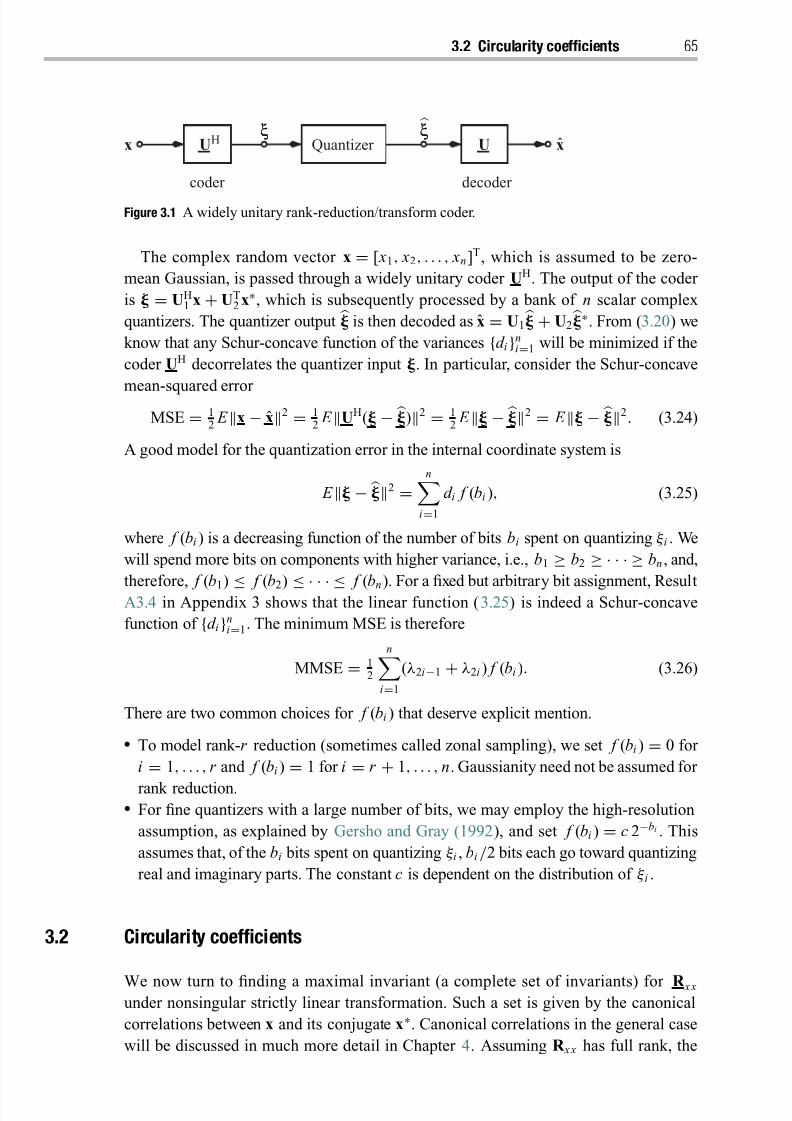
8/21/2019 Statistical Signal Processing of Complex-Valued Data.pdf
http://slidepdf.com/reader/full/statistical-signal-processing-of-complex-valued-datapdf 87/330
3.2 Circularity coefficients 65
decoder coder
Quantizer UUH x
ξξ ξξx
Figure 3.1 A widely unitary rank-reduction/transform coder.
The complex random vector x = [ x1, x2, . . . , xn]T, which is assumed to be zero-
mean Gaussian, is passed through a widely unitary coder UH. The output of the coder
is = UH1 x + UT
2 x∗, which is subsequently processed by a bank of n scalar complex
quantizers. The quantizer output is then decoded as x = U1 + U2
∗. From (3.20) we
know that any Schur-concave function of the variances {d i}ni=1 will be minimized if the
coder UH decorrelates the quantizer input . In particular, consider the Schur-concave
mean-squared error MSE = 1
2 E x − x2 = 1
2 E UH( − )2 = 1
2 E − 2 = E − 2. (3.24)
A good model for the quantization error in the internal coordinate system is
E − 2 =n
i=1
d i f (bi ), (3.25)
where f (bi ) is a decreasing function of the number of bits bi spent on quantizing ξ i . We
will spend more bits on components with higher variance, i.e., b1 ≥ b2 ≥ · · · ≥ bn , and,
therefore, f (b1) ≤ f (b2) ≤ · · · ≤ f (bn). For a fixed but arbitrary bit assignment, ResultA3.4 in Appendix 3 shows that the linear function (3.25) is indeed a Schur-concave
function of {d i}ni=1. The minimum MSE is therefore
MMSE = 12
ni=1
(λ2i−1 + λ2i ) f (bi ). (3.26)
There are two common choices for f (bi ) that deserve explicit mention.
To model rank-r reduction (sometimes called zonal sampling), we set f (bi ) = 0 for
i
=1, . . . , r and f (bi )
=1 for i
=r
+1, . . . , n. Gaussianity need not be assumed for
rank reduction. For fine quantizers with a large number of bits, we may employ the high-resolution
assumption, as explained by Gersho and Gray (1992), and set f (bi ) = c 2−bi . This
assumes that, of the bi bits spent on quantizing ξ i , bi /2 bits each go toward quantizing
real and imaginary parts. The constant c is dependent on the distribution of ξ i .
3.2 Circularity coefficients
We now turn to finding a maximal invariant (a complete set of invariants) for R x x
under nonsingular strictly linear transformation. Such a set is given by the canonical
correlations between x and its conjugate x∗. Canonical correlations in the general case
will be discussed in much more detail in Chapter 4. Assuming R x x has full rank, the
8/21/2019 Statistical Signal Processing of Complex-Valued Data.pdf
http://slidepdf.com/reader/full/statistical-signal-processing-of-complex-valued-datapdf 88/330
66 Second-order description of complex random vectors
canonical correlations between x and x∗ are determined by starting with the coherence
matrix
C
=R −1/2
x x R x x (R ∗ x x )−H/2
=R −1/2
x x R x x R −T/2 x x . (3.27)
Since C is complex symmetric, C = CT, yet not Hermitian symmetric, C = CH, there
exists a special singular value decomposition (SVD), called the Takagi factorization,
which is
C = FKFT. (3.28)
The Takagi factorization is discussed more thoroughly in Section 3.2.2. The complex
matrix F is unitary, and K = Diag(k 1, k 2, . . . , k n) contains the canonical correlations
1 ≥ k 1 ≥ k 2 ≥ · · · ≥ k n ≥ 0 on its diagonal. The squared canonical correlations k 2i are
the eigenvalues of the squared coherence matrix CCH
=R −1/2
x x R x x R −∗ x x R ∗
x x
R −H/2
x x
, or
equivalently, of the matrix R −1 x xR x x R −∗ x x
R ∗ x x because
KK H = FHR −1/2 x x
R x x R −∗ x xR ∗ x x R −H/2
x x F. (3.29)
The canonical correlations between x and x∗ are invariant to the choice of a square
root for R x x , and they are a maximal invariant for R x x under nonsingular strictly linear
transformation of x. Therefore, any function of R x x that is invariant under nonsingular
strictly linear transformation must be a function of these canonical correlations only.
The internal description
= FH
R −1/2
x x x = Ax (3.30)
is said to be given in canonical coordinates. We will adopt the following terminology
by Eriksson and Koivunen (2006).
Definition 3.1. Vectors that are uncorrelated with unit variance, but possibly improper,
are called strongly uncorrelated . The transformation A = FHR −1/2 x x , which transforms x
into canonical coordinates , is called the strong uncorrelating transform (SUT). The
canonical correlations k i are referred to as circularity coefficients , and the set {k i}ni=1
as the circularity spectrum of x.
The term “circularity coefficient” is not entirely accurate insofar as the circularitycoefficients only characterize second-order circularity, or (im-)propriety. Thus, the name
impropriety coefficients would have been more suitable. Moreover, the insight that the
circularity coefficients are canonical correlations is critical because it enables us to
utilize a wealth of results on canonical correlations in the literature.2
The canonical coordinates are strongly uncorrelated, i.e., they are uncorrelated,
E ξ i ξ ∗ j = E ξ i ξ j = 0 for i = j , (3.31)
and have unit variance, E |ξ i |2 = 1. However, they are generally improper as
E ξ 2i = k i . (3.32)
The circularity coefficients k i measure the correlations between the white, unit-
norm canonical coordinates and their conjugates ∗. More precisely, the
8/21/2019 Statistical Signal Processing of Complex-Valued Data.pdf
http://slidepdf.com/reader/full/statistical-signal-processing-of-complex-valued-datapdf 89/330
3.2 Circularity coefficients 67
circularity coefficients k i are the cosines of the canonical angles between the linear
subspaces spanned by and the complex conjugate ∗. If these angles are small,
then x∗ may be linearly estimated from x, indicating that x is improper – obvi-
ously, x∗ can always be perfectly estimated from x if widely linear operations are
allowed. If these angles are large, then x∗ may not be linearly estimated from x,
indicating a proper x. These angles are invariant with respect to nonsingular linear
transformation.
3.2.1 Entropy
Combining our results so far, we may factor R x x as
R x x = R x x R x xR ∗ x x R ∗ x x = R 1/2
x x 0
0 R ∗/2 x x F 0
0 F∗ I K
K I FH 0
0 FT R H/2 x x 0
0 R T/2 x x .
(3.33)
Note that each factor is an augmented matrix. This factorization establishes
det R x x = det2R x x det(I − KK H) = det2R x x
ni=1
(1 − k 2i ). (3.34)
This allows us to derive the following connection between the entropy of an improper
Gaussian random vector with augmented covariance matrix R x x and the corresponding
proper Gaussian random vector with covariance matrix R x x .
Result 3.2. The entropy of a complex improper Gaussian random vector x is
H improper = 12 log[(π e)2n det R x x ]
= log[(πe)n det R x x ] H proper
+ 12 log
ni=1
(1 − k 2i ) − I (x; x∗)
, (3.35)
where H proper is the entropy of a proper Gaussian random vector with the same Her-
mitian covariance matrix R x x (but R x x = 0 ), and I (x; x∗) is the (nonnegative) mutual information between x and x∗. Therefore, the entropy is maximized if and only if x is
proper.
If x is improper, the loss in entropy compared with the proper case is the mutual
information between x and x∗, which is a function of the circularity spectrum.
3.2.2 Strong uncorrelating transform (SUT)
The Takagi factorization is a special SVD for a complex symmetric matrix C = CT.
But why do we need the Takagi factorization C = FKFT rather than simply a regular SVD C = UKVH? The reason is that the canonical coordinates and ∗ are supposed
to be complex conjugates of each other. If we used a regular SVD C = UKVH, then
VHR −∗/2 x x x∗ would not generally be the complex conjugate of = UHR −1/2
x x x. For this
8/21/2019 Statistical Signal Processing of Complex-Valued Data.pdf
http://slidepdf.com/reader/full/statistical-signal-processing-of-complex-valued-datapdf 90/330
68 Second-order description of complex random vectors
we need V = U∗. So how exactly is the Takagi factorization determined from the SVD?
Because the matrix C is symmetric, it has two SVDs:
C
=UKVH
=V∗KUT
=CT. (3.36)
Now, since
CCH = UK 2UH = V∗K 2VT ⇔ K 2UHV∗ = UHV∗K 2
⇔ KUHV∗ = UHV∗K , (3.37)
the unitary matrix UHV∗ commutes with K . This is possible only if the (i, j )th element
of UHV∗ is zero whenever k i = k j . Thus, every C can be expressed as
C = UKDUT (3.38)
with D = VH
U∗. Assume that among the circularity coefficients {k i }n
i=1 there are N dis-tinct coefficients, denoted by σ 1, . . . , σ N . Their respective multiplicities are m1, . . . , m N .
Then we may write
D = Diag(D1, D2, . . . , D N ), (3.39)
where Di is an m i × mi unitary and symmetric matrix, and
KD = Diag(σ 1D1, σ 2D2, . . . , σ N D N ). (3.40)
In the special case in which all circularity coefficients are distinct, we have σ i = k i
and Di is a scalar with unit magnitude. Therefore,
D = Diag(e jθ 1 , e jθ 2 , . . . , e jθ n ) (3.41)
KD = Diag(k 1e jθ 1 , k 2e jθ 2 , . . . , k ne jθ n ). (3.42)
Then we have
C = UD1/2KDT/2UT (3.43)
with
D1/2
=Diag(
±e jθ 1/2,
±e jθ 2/2, . . . ,
±e jθ n /2) (3.44)
with arbitrary signs, so that F = UD1/2 achieves the Takagi factorization C = FKFT.
This shows how to obtain the Takagi factorization from the SVD. We note that, if only
the circularity coefficients k i need to be computed and the canonical coordinates are
not required, a regular SVD will suffice.
The SVD C = UKVH of any matrix C with distinct singular values is unique up to
multiplication of U from the right by a unitary diagonal matrix. If C = CT, the Takagi
factorization determines this unitary diagonal factor in such a way that the matrix of
left singular vectors is the conjugate of the matrix of right singular vectors. Hence, if all
circularity coefficients are distinct, the Takagi factorization is unique up to the sign of
the diagonal elements in D1/2. The following result then follows.
Result 3.3. For distinct circularity coefficients, the strong uncorrelating transformA =FHR −1/2
x x is unique up to the sign of its rows, regardless of the choice of the inverse
square root of R x x .
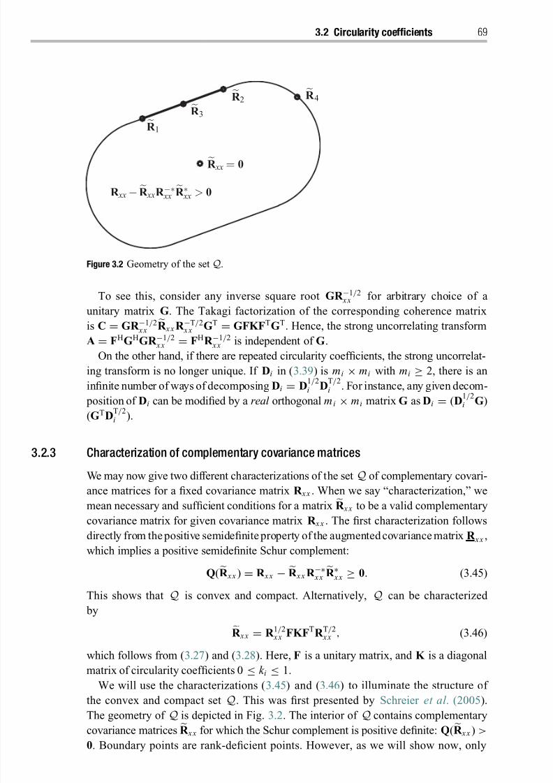
8/21/2019 Statistical Signal Processing of Complex-Valued Data.pdf
http://slidepdf.com/reader/full/statistical-signal-processing-of-complex-valued-datapdf 91/330
3.2 Circularity coefficients 69
R xx− R xxR −∗ xx R ∗ xx > 0
R 4R 2
R 3
R 1
R xx = 0
Figure 3.2 Geometry of the set
Q.
To see this, consider any inverse square root GR −1/2 x x for arbitrary choice of a
unitary matrix G. The Takagi factorization of the corresponding coherence matrix
is C = GR −1/2 x x
R x x R −T/2 x x GT = GFKFTGT. Hence, the strong uncorrelating transform
A = FHGHGR −1/2 x x = FHR −1/2
x x is independent of G.
On the other hand, if there are repeated circularity coefficients, the strong uncorrelat-
ing transform is no longer unique. If Di in (3.39) is mi × mi with mi ≥ 2, there is an
infinite number of ways of decomposing Di = D1/2i D
T/2i . For instance, any given decom-
position of Di can be modified by a real orthogonal m i
×mi matrix G as Di
=(D
1/2i G)
(GTDT/2i ).
3.2.3 Characterization of complementary covariance matrices
We may now give two different characterizations of the set Q of complementary covari-
ance matrices for a fixed covariance matrix R x x . When we say “characterization,” we
mean necessary and sufficient conditions for a matrix R x x to be a valid complementary
covariance matrix for given covariance matrix R x x . The first characterization follows
directly from thepositive semidefiniteproperty of the augmented covariance matrix R x x ,
which implies a positive semidefinite Schur complement:
Q(R x x ) = R x x − R x x R −∗ x xR ∗ x x ≥ 0. (3.45)
This shows that Q is convex and compact. Alternatively, Q can be characterized
by R x x = R 1/2 x x FKFTR T/2
x x , (3.46)
which follows from (3.27) and (3.28). Here, F is a unitary matrix, and K is a diagonal
matrix of circularity coefficients 0 ≤ k i ≤ 1.
We will use the characterizations (3.45) and (3.46) to illuminate the structure of the convex and compact set Q. This was first presented by Schreier et al . (2005).
The geometry of Q is depicted in Fig. 3.2. The interior of Q contains complementary
covariance matrices R x x for which the Schur complement is positive definite: Q(R x x ) >
0. Boundary points are rank-deficient points. However, as we will show now, only
8/21/2019 Statistical Signal Processing of Complex-Valued Data.pdf
http://slidepdf.com/reader/full/statistical-signal-processing-of-complex-valued-datapdf 92/330
70 Second-order description of complex random vectors
boundary points where the Schur complement is identically zero, Q(R x x ) = 0, are also
extreme points.
Definition 3.2. An extreme point R # of the closed convex set
Q may be written as a
convex combination of points inQ in only a trivial way. That is, if R # = αR 1 + (1 − α)R 2
with 0 < α < 1 , R 1, R 2 ∈ Q , then R # = R 1 = R 2.
In Fig. 3.2, only R 4 is an extreme point. The boundary point R 3, for instance, can be
obtained as a convex combination of the points R 1 and R 2.
Result 3.4. A complementary covariance matrix R # is an extreme point of Q if and only
if the Schur complement of R x x vanishes: Q(R #) = 0. In other words, R # is an extreme
point if and only if all circularity coefficients have unit value: k i = 1 , i = 1, . . . , n.
We prove this result by first showing that a point R x x
∈ Qwith nonzero Schur com-
plement cannot be an extreme point. There exists at least one circularity coefficient, say
k j , with k j < 1. Now choose ε > 0 such that k j + ε ≤ 1. Define K 1 such that it agrees
with K except that the j th entry, k j , is replaced with k j + ε. Similarly, define K 2 such
that it agrees with K except that the j th entry, k j , is replaced with k j − ε. Then, using
(3.46), write R x x = 12
R 1/2 x x F(K 1 + K 2)FTR T/2
x x (3.47)
= 12
R 1 + 1
2
R 2. (3.48)
This expresses R x x as a nontrivial convex combination of R 1 = R 1/2 x x FK 1F
T
R T/2 x x and R 2 = R 1/2
x x FK 2FTR T/2 x x , with α = 1/2. Hence, R x x is not an extreme point.
We now assume that the Schur complement Q(R x x ) = R x x − R x x R −∗ x xR ∗ x x = 0 for
some R x x . We first note that
α(1 − α)(R 1 − R 2)R −∗ x x (R 1 − R 2)H ≥ 0 (3.49)
with equality if and only if R 1 = R 2. This implies
(α
R 1 + (1 − α)
R 2)R x x (α
R 1 + (1 − α)
R 2)∗ ≤ α
R 1R x x
R ∗1 + (1 − α)
R 2R x x
R ∗2.
(3.50)
Thus, we find
α Q(R 1) + (1 − α)Q(R 2) ≤ Q(R x x ) (3.51)
for R x x = αR 1 + (1 − α)R 2, with equality if and only if R 1 = R 2. This makes Q(R x x )
a strictly matrix-concave function. Since Q(R 1) ≥ 0 and Q(R 2) ≥ 0, a vanishing
Q(R x x ) = 0 requires R 1 = R 2 = R x x . Thus, R x x is indeed an extreme point of Q,
which concludes the proof of the result.
3.3 Degree of impropriety
Building upon our insights from the previous section, we may now ask how to quantify
the degree of impropriety of x. Propriety is preserved by strictly linear (but not widely
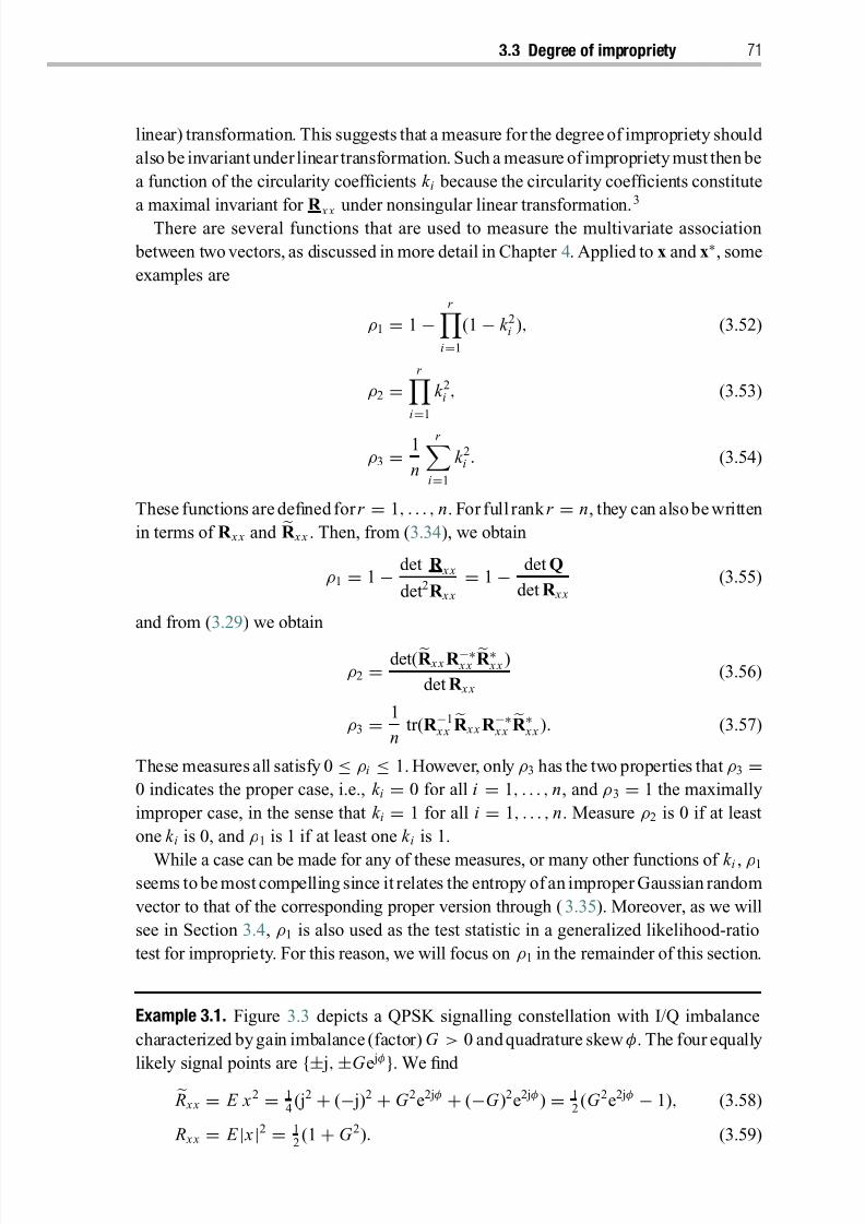
8/21/2019 Statistical Signal Processing of Complex-Valued Data.pdf
http://slidepdf.com/reader/full/statistical-signal-processing-of-complex-valued-datapdf 93/330
3.3 Degree of impropriety 71
linear) transformation. This suggests that a measure for the degree of impropriety should
also be invariant under linear transformation. Such a measure of impropriety must then be
a function of the circularity coefficients k i because the circularity coefficients constitute
a maximal invariant for R x x
under nonsingular linear transformation.3
There are several functions that are used to measure the multivariate association
between two vectors, as discussed in more detail in Chapter 4. Applied to x and x∗, some
examples are
ρ1 = 1 −r
i=1
(1 − k 2i ), (3.52)
ρ2 =r
i=1
k 2i , (3.53)
ρ3 =1
n
r i=1
k 2i . (3.54)
These functions are defined for r = 1, . . . , n. For full rank r = n, they can also bewritten
in terms of R x x and R x x . Then, from (3.34), we obtain
ρ1 = 1 − det R x x
det2R x x
= 1 − det Q
det R x x
(3.55)
and from (3.29) we obtain
ρ2 =det(R x x R −∗ x x
R ∗ x x )
det R x x
(3.56)
ρ3 =1
ntr(R −1
x xR x x R −∗ x x
R ∗ x x ). (3.57)
These measures all satisfy 0 ≤ ρi ≤ 1. However, only ρ3 has the two properties that ρ3 =0 indicates the proper case, i.e., k i = 0 for all i = 1, . . . , n, and ρ3 = 1 the maximally
improper case, in the sense that k i = 1 for all i = 1, . . . , n. Measure ρ2 is 0 if at least
one k i is 0, and ρ1 is 1 if at least one k i is 1.
While a case can be made for any of these measures, or many other functions of k i , ρ1
seems to be most compelling since it relates the entropy of an improper Gaussian random
vector to that of the corresponding proper version through (3.35). Moreover, as we will
see in Section 3.4, ρ1 is also used as the test statistic in a generalized likelihood-ratio
test for impropriety. For this reason, we will focus on ρ1 in the remainder of this section.
Example 3.1. Figure 3.3 depicts a QPSK signalling constellation with I/Q imbalance
characterized by gain imbalance (factor) G > 0 and quadrature skew φ. The four equally
likely signal points are{±
j,±
G e jφ
}. We find R x x = E x2 = 1
4(j2 + (− j)2 + G 2e2jφ + (−G )2e2jφ) = 1
2(G 2e2jφ − 1), (3.58)
R x x = E | x|2 = 12(1 + G 2). (3.59)
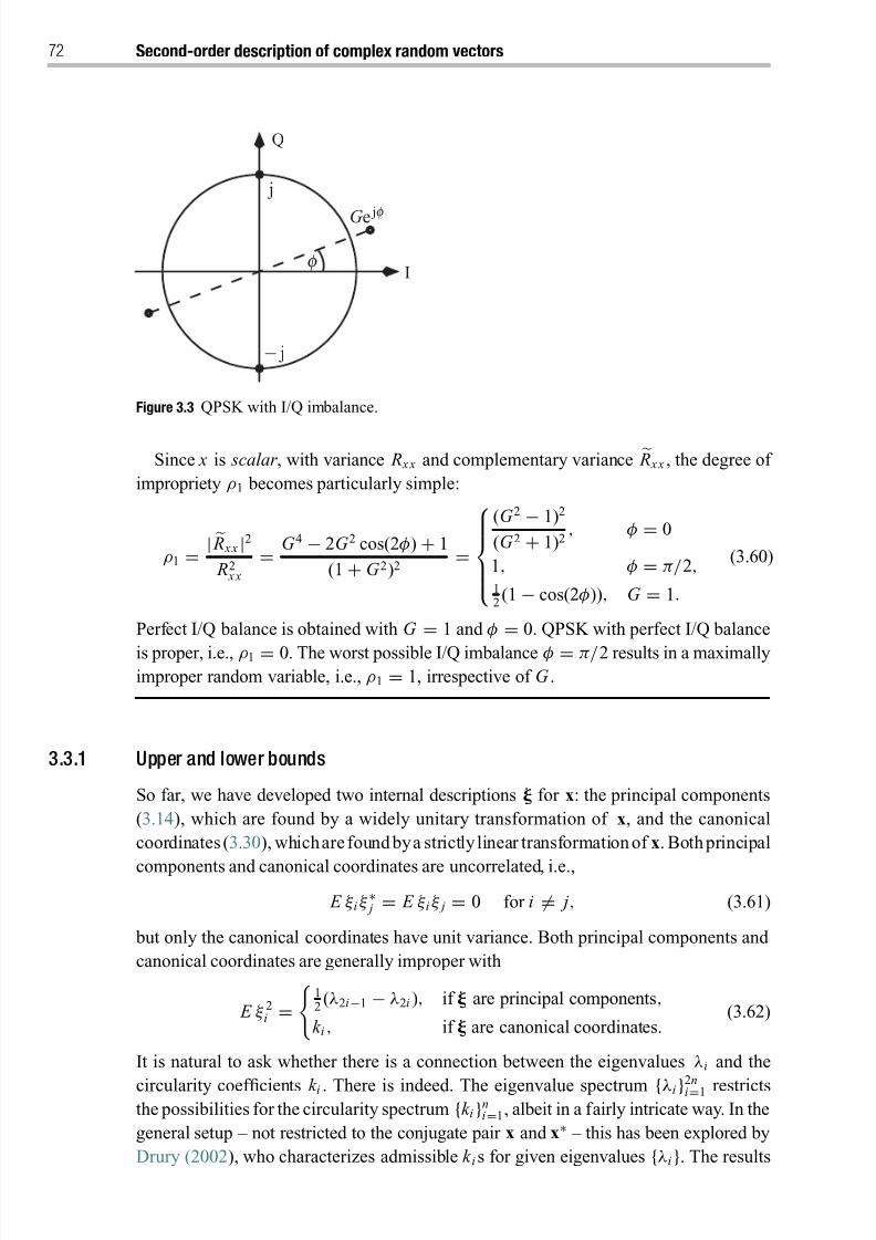
8/21/2019 Statistical Signal Processing of Complex-Valued Data.pdf
http://slidepdf.com/reader/full/statistical-signal-processing-of-complex-valued-datapdf 94/330
72 Second-order description of complex random vectors
I
Q
f
j
− j
G e jf
Figure 3.3 QPSK with I/Q imbalance.
Since x is scalar , with variance R x x and complementary variance R x x , the degree of
impropriety ρ1 becomes particularly simple:
ρ1 =| R x x |2
R2 x x
= G 4 − 2G 2 cos(2φ) + 1
(1 + G 2)2 =
(G 2 − 1)2
(G 2 + 1)2, φ = 0
1, φ = π/2,
12(1 − cos(2φ)), G = 1.
(3.60)
Perfect I/Q balance is obtained with G
=1 and φ
=0. QPSK with perfect I/Q balance
is proper, i.e., ρ1 = 0. The worst possible I/Q imbalance φ = π/2 results in a maximallyimproper random variable, i.e., ρ1 = 1, irrespective of G .
3.3.1 Upper and lower bounds
So far, we have developed two internal descriptions for x: the principal components
(3.14), which are found by a widely unitary transformation of x, and the canonical
coordinates (3.30), whicharefound bya strictly linear transformation of x. Both principal
components and canonical coordinates are uncorrelated, i.e.,
E ξ i ξ ∗ j = E ξ i ξ j = 0 for i = j , (3.61)
but only the canonical coordinates have unit variance. Both principal components and
canonical coordinates are generally improper with
E ξ 2i =
12(λ2i−1 − λ2i ), if are principal components,
k i , if are canonical coordinates.(3.62)
It is natural to ask whether there is a connection between the eigenvalues λi and the
circularity coefficients k i . There is indeed. The eigenvalue spectrum {λi}2ni=1 restrictsthe possibilities for the circularity spectrum {k i }n
i=1, albeit in a fairly intricate way. In the
general setup – not restricted to the conjugate pair x and x∗ – this has been explored by
Drury (2002), who characterizes admissible k i s for given eigenvalues {λi}. The results
8/21/2019 Statistical Signal Processing of Complex-Valued Data.pdf
http://slidepdf.com/reader/full/statistical-signal-processing-of-complex-valued-datapdf 95/330
3.3 Degree of impropriety 73
are very involved, which is due to the fact that the singular values of the sum of two
matrices are not easily characterized. It is much easier to develop bounds on certain
functions of {k i} in terms of the eigenvalues {λi}. In particular, we are interested in
bounds on the degree of impropriety ρ1 if {
λi}
are known. We first state the upper bound
on ρ1.
Result 3.5. The degree of impropriety ρ1 of a vector x with prescribed eigenvalues {λi}of the augmented covariance matrix R x x is upper-bounded by
ρ1 = 1 −r
i=1
(1 − k 2i ) ≤ 1 −r
i=1
4λi λ2n+1−i
(λi + λ2n+1−i )2, r = 1, . . . , n. (3.63)
This upper bound is attained when
R x x = 12 Diag(λ1 + λ2n , λ2 + λ2n−1, . . . , λn + λn+1), (3.64)R x x = 12
Diag(λ1 − λ2n , λ2 − λ2n−1, . . . , λn − λn+1). (3.65)
This bound has been derived by Bartmann and Bloomfield (1981) for the canonical
correlations between arbitrary pairs of real vectors (u, v), and it holds a forteriori for the
canonical correlations between x and x∗. It is easy to see that R x x , with R x x and R x x as
specified in (3.64) and (3.65), is a valid augmented covariance matrix with eigenvalues
{λi} and attains the bound.
There is no nontrivial lower bound on the canonical correlations between arbitrary
pairs of random vectors (x, y). It is always possible to choose, for instance, E xxH =Diag(λ1, . . . , λn), E yyH = Diag(λn+1, . . . , λ2n), and E xyH = 0, which has the required
eigenvalues {λi} and zero canonical correlation matrix K = 0. That there is a lower
bound on ρ1 stems from the special structure of the augmented covariance matrix R x x ,
where the northwest and southeast blocks must be complex conjugates.
We will now derive this lower bound for r = n. Let x = u + jv and z = [uT, vT]T.
From (2.21) and (2.22), we know that
R x x = R uu + R vv + j(R Tuv − R uv), (3.66)
R x x = R uu − R vv + j(R Tuv + R uv). (3.67)
Since the eigenvalues are given,
det R x x =2n
i=1
λi (3.68)
is fixed. Hence, it follows from (3.34) that the minimum ρ1 is achieved when det R x x
is minimized. We can assume without loss of generality that R x x is diagonal. If it is
not, it can be made diagonal with a strictly unitary transform that leaves det R x x and the
eigenvalues {λi} unchanged. Thus, we have
min det R x x = min
ni=1
(R x x )ii = min
ni=1
[(R uu )ii + (R vv )ii ]. (3.69)

8/21/2019 Statistical Signal Processing of Complex-Valued Data.pdf
http://slidepdf.com/reader/full/statistical-signal-processing-of-complex-valued-datapdf 96/330
74 Second-order description of complex random vectors
Now let qi be the i th largest diagonal element of R uu + R vv , and r i the i th largest
diagonal element of R zz . Then,
r
i=1
qi ≤r
i=1
r 2i−1 + r 2i ≤r
i=1
λ2i
−1
+λ2i
2 , r = 1, . . . , n, (3.70)
with equality for r = n. We have the second inequality because the diagonal ele-
ments of R zz are majorized by the eigenvalues of R zz (cf. Result A3.5). Since
qi
is Schur-concave, a consequence of (3.70) is the following variant of Hadamard’s
inequality:
ni=1
[(R uu )i i + (R vv )i i ] ≥n
i=1
λ2i−1 + λ2i
2 . (3.71)
This implies
min det R x x =n
i=1
λ2i−1 + λ2i
2 . (3.72)
Using this result in (3.34), we get
n
i=1
(1
−k 2i )
≤
2ni=1
λi
ni=1
(λ2i−1 + λ2i )2
4
, (3.73)
from which we obtain the following lower bound on ρ1.
Result 3.6. The degree of impropriety ρ1 of a vector x with prescribed eigenvalues {λi}of the augmented covariance matrix R x x is lower-bounded by
ρ1 = 1 −n
i=1
(1 − k 2i ) ≥ 1 −n
i=1
4λ2i−1λ2i
(λ2i−1 + λ2i )2. (3.74)
The lower bound is attained if R uu = 12Λ
(1) , R vv = 12Λ
(2) , and R uv = 0 , or, equivalently,
R x x = 12(Λ(1) +Λ(2)) = 1
2 Diag (λ1 + λ2, λ3 + λ4, . . . , λ2n−1 + λ2n), (3.75)R x x = 1
2(Λ(1) −Λ(2)) = 1
2 Diag(λ1 − λ2, λ3 − λ4, . . . , λ2n−1 − λ2n), (3.76)
whereΛ(1) = Diag(λ1, λ3, . . . , λ2n−1) and Λ(2) = Diag(λ2, λ4, . . . , λ2n).
Example 3.2. In the scalar case n
=1, the upper bound equals the lower bound, which
leads to the following expression for the degree of impropriety:
ρ1 = k 21 = 1 − 4λ1λ2
(λ1 + λ2)2 = (λ1 − λ2)2
(λ1 + λ2)2.
8/21/2019 Statistical Signal Processing of Complex-Valued Data.pdf
http://slidepdf.com/reader/full/statistical-signal-processing-of-complex-valued-datapdf 97/330
3.3 Degree of impropriety 75
Thus we also have a simple expression for the circularity coefficient k 1 in terms of the
eigenvalues λ1 and λ2:
k 1 =
λ1 − λ2
λ1 + λ2
.
While the upper bound (3.63) holds for r = 1, . . . , n, we have been able to establish
the lower bound (3.74) for r = n only. A natural conjecture is to assume that the diagonal
R x x and R x x given by (3.75) and (3.76) also attain the lower bound for r < n . Let ci be
the i th largest of the factors
4λ2 j −1λ2 j
(λ2 j −1 + λ2 j )2, j = 1, . . . , n.
Then the conjecture may be written as
ρ1 = 1 −r
i=1
(1 − k 2i ) ≥ 1 −n
i=n−r +1
ci , r = 1, . . . , n. (3.77)
We point out that the diagonal matrices R x x and R x x that achieve the upper bound do
not necessarily give upper bounds for other functions of {k i}, such as ρ2 and ρ3. Drury
et al . (2002) prove an upper bound for ρ2 and conjecture an upper bound for ρ3. Lower
bounds for ρ2 and ρ3 are still unresolved problems.
Example 3.3. We have seen that the principal components minimize the degree of impro-
priety ρ1 under widely unitary transformation. In this example, we show that they do
not necessarily minimize other measures of impropriety such as ρ2 and ρ3.
Consideran augmentedcovariance matrix R x x with eigenvalues 100, 50, 50,and2.The
principal components have covariance matrix R ξ ξ = Diag(75, 26), complementary
covariance matrix R ξ ξ = Diag(25, 24), and circularity coefficients k 1 = 24/26 and k 2 =25/75. We compute ρ2 = 0.481 and ρ3 = 0.095.
On the other hand, there obviously exists a widely unitary transformation into coor-
dinates x with covariance matrix R x x = Diag(51, 50) and complementary covariancematrix R x x = Diag(49, 0), and circularity coefficients k 1 = 49/51 and k 2 = 0/50. The
description x is less improper than the principal components when measured in terms
of ρ2 = 0.461 and ρ3 = 0.
Least improper analog
Given a random vector x, we can produce a least improper analog = UHx, using a
widely unitary transformation U. It is clear from (3.75) and (3.76) that the principal
components obtained from (3.14) are such an analog, with U determined by the EVDR x x = UΛUH. The principal components have the same eigenvalues and thus the
same power as x. They minimize ρ1 and thus maximize entropy under widely unitary
transformation. We note that a least improper analog is not unique, since any strictly
8/21/2019 Statistical Signal Processing of Complex-Valued Data.pdf
http://slidepdf.com/reader/full/statistical-signal-processing-of-complex-valued-datapdf 98/330
76 Second-order description of complex random vectors
unitary transform will leave both the eigenvalues {λi } and the canonical correlations {k i}unchanged.
3.3.2 Eigenvalue spread of the augmented covariance matrix
Let us try to further illuminate the upper and lower bounds. Both the upper and
the lower bounds are attained when R x x and R x x are diagonal matrices. For R x x =Diag( R11, . . . , Rnn ) and R x x = Diag( R11, . . . , Rnn ), we find that
ni=1
(1 − k 2i ) =n
i=1
1 − | Rii |2
R2ii
. (3.78)
If R x x has diagonal blocks R x x and R x x , it has eigenvalues
{ Rii
± | Ri i
|}ni
=1. This gives
ni=1
(1 − k 2i ) =n
i=1
1 − (ai − bi )
2
(ai + bi )2
=
ni=1
4ai bi
(ai + bi )2, (3.79)
where {ai }ni=1 and {bi }n
i=1 are two disjoint subsets of {λi}2ni=1. Each factor
4ai bi
(ai + bi )2
is the squared ratio of the geometric and arithmetic means of ai and bi . Hence, it is
1 if ai
=bi , and 0 if ai or bi are 0, and thus measures the spread between ai and
bi . Minimizing or maximizing (3.79) is a matter of choosing the subsets {ai} and {bi}from the eigenvalues {λi } using a combinatorial argument presented by Bloomfield and
Watson (1975). In order to minimize (3.79), we need maximum spread between the two
sets {ai} and {bi }, which is achieved by choosing ai = λi and bi = λ2n−i . In order to
maximize (3.79), we need minimum spread between {ai } and {bi}, which is achieved by
ai = λ2i−1 and bi = λ2i . Hence, the degree of impropriety is related to the eigenvalue
spread of R x x .
3.3.3 Maximally improper vectorsFollowing this line of thought, one might expect a vector that is maximally improper – in
the sense that K = I – to correspond to an augmented covariance matrix with maximum
possible eigenvalue spread. This was in fact claimed by Schreier et al . (2005) but,
unfortunately, it is only partially true. Let ev(R x x ) = [µ1, µ2, . . . , µn]T and ev(R x x ) =[λ1, λ2, . . . , λ2n]. Let R # be the augmented covariance matrix of a maximally improper
vector with K = I. Using (3.46), we may write
R # = R x x R 1/2
x x FFTR T/2 x x
R ∗/2
x x
F∗FHR H/2
x x
R ∗ x x (3.80)
for some unitary matrix F. The matrix R # has a vanishing Schur complement and thusR # = R 1/2 x x FFTR T/2
x x is an extreme point in the set Q. Schreier et al . (2005) incorrectly
stated that ev(R #) = [2µ1, 2µ2, . . . , 2µn , 0Tn ]T for any extremepoint R #. While this isnot
8/21/2019 Statistical Signal Processing of Complex-Valued Data.pdf
http://slidepdf.com/reader/full/statistical-signal-processing-of-complex-valued-datapdf 99/330
3.4 Testing for impropriety 77
true, there is indeed at least one extreme point R ## such that the augmented covariance
matrix R ## has these eigenvalues. Let R x x = UMUH be the EVD of R x x . Choosing
R ##
=UMUT
=UM1/2UHUUTU∗M1/2UT
=R 1/2
x x FFTR T/2 x x (3.81)
with F = U means that
R ## =
R x x R ##R ∗## R ∗ x x
(3.82)
has eigenvalues ev(R ##) = [2µ1, 2µ2, . . . , 2µn , 0Tn ]T. Letus now establish the following.
Result 3.7. There is the majorization preordering
ev(R 0) ≺ ev(R x x ) ≺ ev(R ##). (3.83)
This says that, for given Hermitian covariance matrix R x x , the vector whose augmented
covariance matrix R x x has least eigenvalue spread must be proper: R x x = 0 and R 0 =Diag(R x x , R ∗ x x ). The vector whose augmented covariance matrix R x x has maximum
eigenvalue spread must be maximally improper, i.e., K = I.
In order to show this result we note that the left inequality is (3.23), and the right
inequality is a consequence of Result A3.8. Applied to the matrix R x x , Result A3.8 says
that
k
i=1
λi +
λ2n−k +i ≤
k
i=1
2µi, k
=1, . . . , n, (3.84)
and, since λ2n−k +i ≥ 0,
k i=1
λi ≤k
i=1
2µi , k = 1, . . . , n. (3.85)
Moreover, the trace constraint tr R x x = 2 tr R x x and λi ≥ 0 imply
k
i=1
λi ≤n
i=1
2µi , k = n + 1, . . . , 2n. (3.86)
Together, (3.85) and (3.86) prove the result.
Again, K = I is a necessary condition only for maximum eigenvalue spread of R x x .
It is not sufficient, as Schreier et al . (2005) incorrectly claimed. In Section 5.4.2, we will
use (3.83) to maximize/minimize Schur-convex/concave functions of ev(R x x ) for fixed
R x x . It follows from (3.83) that these maxima/minima will be achieved for the extreme
point R ##, but not necessarily for all extreme points.
3.4 Testing for impropriety
In practice, the complementary covariance matrix must often be estimated from the data
available. Such an estimate will in general be nonzero even if the source is actually
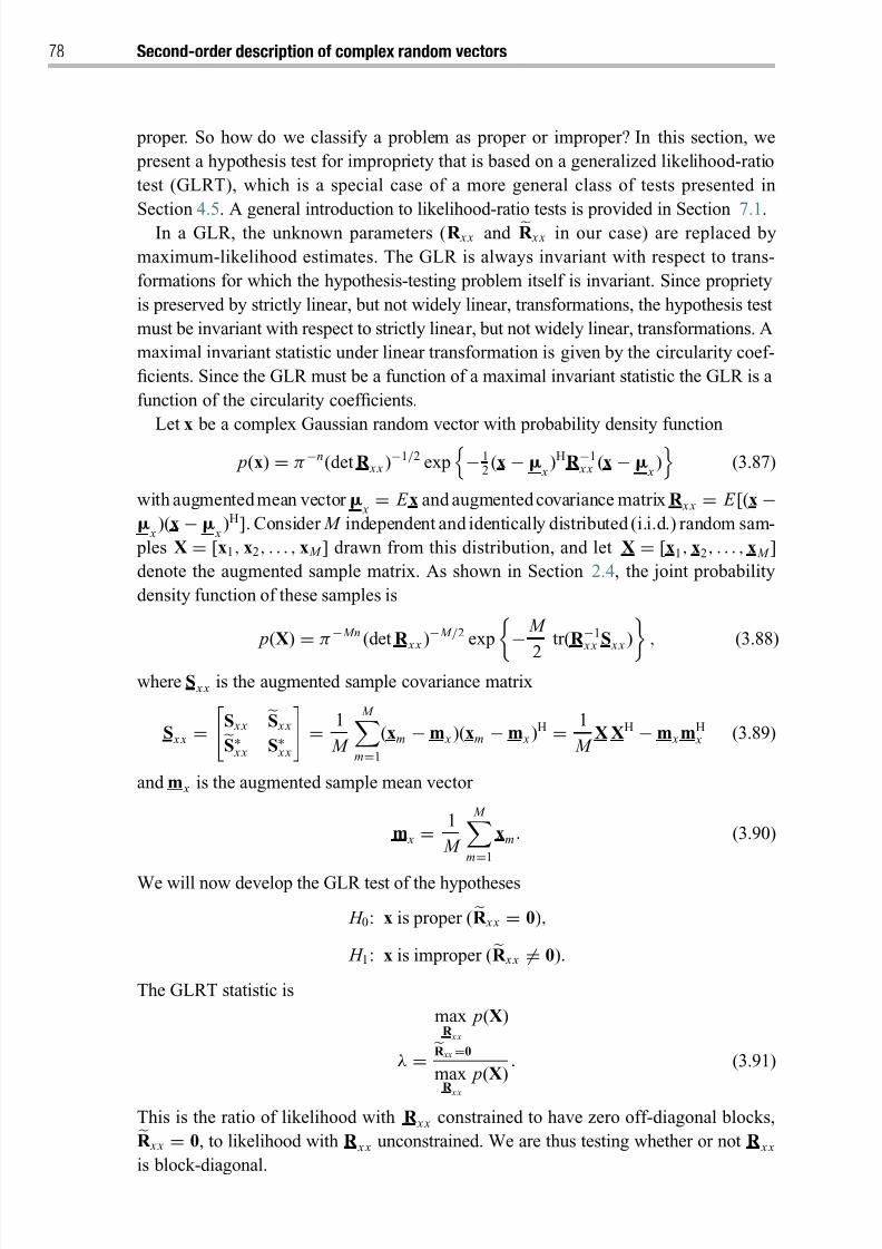
8/21/2019 Statistical Signal Processing of Complex-Valued Data.pdf
http://slidepdf.com/reader/full/statistical-signal-processing-of-complex-valued-datapdf 100/330
78 Second-order description of complex random vectors
proper. So how do we classify a problem as proper or improper? In this section, we
present a hypothesis test for impropriety that is based on a generalized likelihood-ratio
test (GLRT), which is a special case of a more general class of tests presented in
Section 4.5. A general introduction to likelihood-ratio tests is provided in Section 7.1.
In a GLR, the unknown parameters (R x x and R x x in our case) are replaced by
maximum-likelihood estimates. The GLR is always invariant with respect to trans-
formations for which the hypothesis-testing problem itself is invariant. Since propriety
is preserved by strictly linear, but not widely linear, transformations, the hypothesis test
must be invariant with respect to strictly linear, but not widely linear, transformations. A
maximal invariant statistic under linear transformation is given by the circularity coef-
ficients. Since the GLR must be a function of a maximal invariant statistic the GLR is a
function of the circularity coefficients.
Let x be a complex Gaussian random vector with probability density function
p(x) = π−n(det R x x )−1/2 exp− 1
2(x −
x)HR −1
x x (x − x
)
(3.87)
with augmented mean vector x = E x and augmented covariance matrix R x x = E [(x −
x
)(x − x
)H]. Consider M independent and identically distributed (i.i.d.) random sam-
ples X = [x1, x2, . . . , x M ] drawn from this distribution, and let X = [x1, x2, . . . , x M ]
denote the augmented sample matrix. As shown in Section 2.4, the joint probability
density function of these samples is
p(X)
=π− Mn (det R x x )− M /2 exp−
M
2
tr(R −1 x x S x x ) , (3.88)
where S x x is the augmented sample covariance matrix
S x x =
S x x S x xS∗
x x S∗ x x
= 1
M
M m=1
(xm − m x )(xm − m x )H = 1
M X XH − m x mH
x (3.89)
and m x is the augmented sample mean vector
m x =1
M
M
m=1
xm . (3.90)
We will now develop the GLR test of the hypotheses
H 0: x is proper (R x x = 0),
H 1: x is improper (R x x = 0).
The GLRT statistic is
λ =
maxR
x x
R xx =0
p(X)
maxR
x x
p(X). (3.91)
This is the ratio of likelihood with R x x constrained to have zero off-diagonal blocks,R x x = 0, to likelihood with R x x unconstrained. We are thus testing whether or not R x x
is block-diagonal.
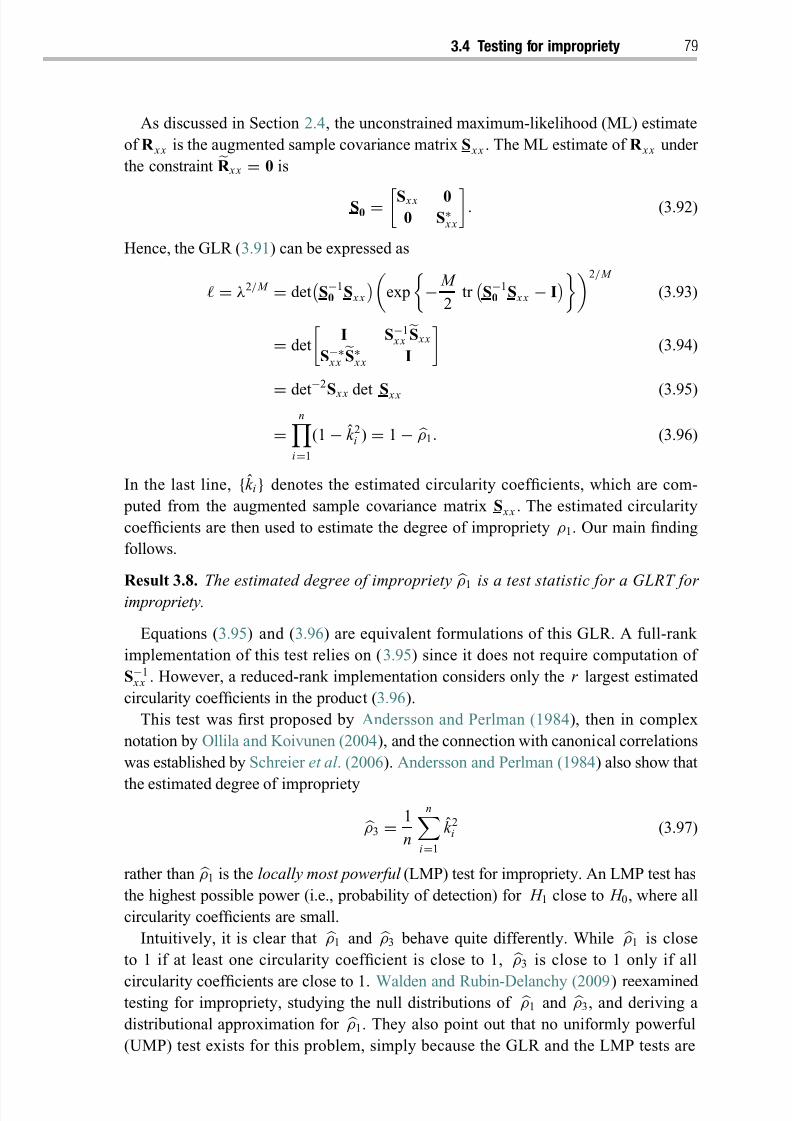
8/21/2019 Statistical Signal Processing of Complex-Valued Data.pdf
http://slidepdf.com/reader/full/statistical-signal-processing-of-complex-valued-datapdf 101/330
3.4 Testing for impropriety 79
As discussed in Section 2.4, the unconstrained maximum-likelihood (ML) estimate
of R x x is the augmented sample covariance matrix S x x . The ML estimate of R x x under
the constraint
R x x = 0 is
S0 = S x x 00 S∗
x x
. (3.92)
Hence, the GLR (3.91) can be expressed as
= λ2/ M = det
S−10 S x x
exp
− M
2 tr
S−10 S x x − I
2/ M
(3.93)
= det
I S−1
x xS x x
S−∗ x x
S∗
x x I
(3.94)
= det−2
S x x det S x x (3.95)
=n
i=1
(1 − k 2i ) = 1 − ρ1. (3.96)
In the last line, {k i } denotes the estimated circularity coefficients, which are com-
puted from the augmented sample covariance matrix S x x . The estimated circularity
coefficients are then used to estimate the degree of impropriety ρ1. Our main finding
follows.
Result 3.8. The estimated degree of impropriety ρ1 is a test statistic for a GLRT for
impropriety.
Equations (3.95) and (3.96) are equivalent formulations of this GLR. A full-rank
implementation of this test relies on (3.95) since it does not require computation of
S−1 x x . However, a reduced-rank implementation considers only the r largest estimated
circularity coefficients in the product (3.96).
This test was first proposed by Andersson and Perlman (1984), then in complex
notation by Ollila and Koivunen (2004), and the connection with canonical correlations
was established by Schreier et al . (2006). Andersson and Perlman (1984) also show that
the estimated degree of impropriety
ρ3 =1
n
ni=1
k 2i (3.97)
rather than ρ1 is the locally most powerful (LMP) test for impropriety. An LMP test has
the highest possible power (i.e., probability of detection) for H 1 close to H 0, where all
circularity coefficients are small.
Intuitively, it is clear that
ρ1 and
ρ3 behave quite differently. While
ρ1 is close
to 1 if at least one circularity coefficient is close to 1, ρ3 is close to 1 only if all
circularity coefficients are close to 1. Walden and Rubin-Delanchy (2009) reexamined testing for impropriety, studying the null distributions of ρ1 and ρ3, and deriving a
distributional approximation for ρ1. They also point out that no uniformly powerful
(UMP) test exists for this problem, simply because the GLR and the LMP tests are
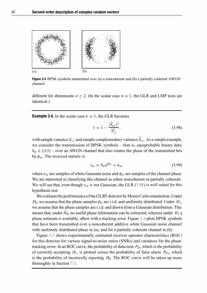
8/21/2019 Statistical Signal Processing of Complex-Valued Data.pdf
http://slidepdf.com/reader/full/statistical-signal-processing-of-complex-valued-datapdf 102/330
80 Second-order description of complex random vectors
(a) (b)
Figure 3.4 BPSK symbols transmitted over (a) a noncoherent and (b) a partially coherent AWGN
channel.
different for dimensions n ≥ 2. (In the scalar case n = 1, the GLR and LMP tests are
identical.)
Example 3.4. In the scalar case n = 1, the GLR becomes
= 1 − |S x x |2S 2 x x
, (3.98)
withsample variance S x x and sample complementary variance S x x . As a simpleexample,
we consider the transmission of BPSK symbols – that is, equiprobable binary data
bm
∈ {±1} – over an AWGN channel that also rotates the phase of the transmitted bits
by φm . The received statistic is
xm = bme jφm + nm , (3.99)
where nm are samples of white Gaussian noise and φm are samples of the channel phase.
We are interested in classifying this channel as either noncoherent or partially coherent.
We will see that, even though x m is not Gaussian, the GLR (3.98) is well suited for this
hypothesis test.
We evaluatetheperformance of the GLRT detector by MonteCarlo simulations. Under
H 0, we assume that the phase samples φm are i.i.d. and uniformly distributed. Under H 1,
we assume that the phase samples are i.i.d. and drawn from a Gaussian distribution. This
means that, under H 0, no useful phase information can be extracted, whereas under H 1 a
phase estimate is available, albeit with a tracking error. Figure 3.4 plots BPSK symbols
that have been transmitted over a noncoherent additive white Gaussian noise channel
with uniformly distributed phase in (a), and for a partially coherent channel in (b).
Figure 3.5 shows experimentally estimated receiver operator characteristics (ROC)
for this detector for various signal-to-noise ratios (SNRs) and variances for the phase
tracking error. In an ROC curve, the probability of detection P D, which is the probability
of correctly accepting H 1, is plotted versus the probability of false alarm P FA, which
is the probability of incorrectly rejecting H 0. The ROC curve will be taken up morethoroughly in Section 7.3.
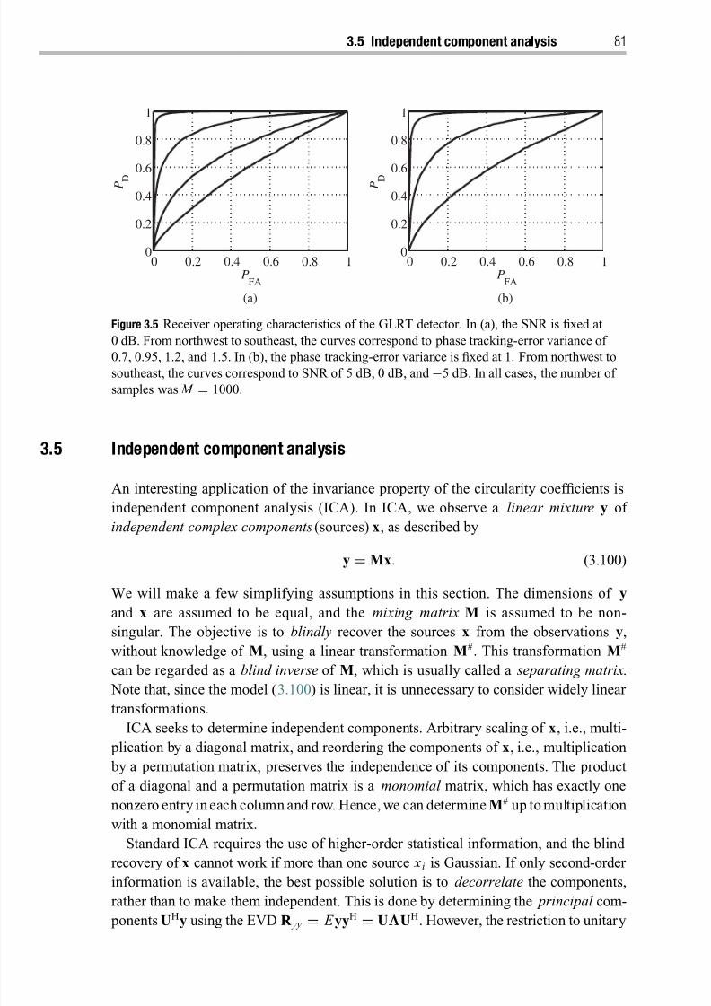
8/21/2019 Statistical Signal Processing of Complex-Valued Data.pdf
http://slidepdf.com/reader/full/statistical-signal-processing-of-complex-valued-datapdf 103/330
3.5 Independent component analysis 81
0 0.2 0.4 0.6 0.8 10
0.2
0.4
0.6
0.8
1
PFA
P D
0 0.2 0.4 0.6 0.8 10
0.2
0.4
0.6
0.8
1
PFA
P D
(a) (b)
Figure 3.5 Receiver operating characteristics of the GLRT detector. In (a), the SNR is fixed at
0 dB. From northwest to southeast, the curves correspond to phase tracking-error variance of
0.7, 0.95, 1.2, and 1.5. In (b), the phase tracking-error variance is fixed at 1. From northwest tosoutheast, the curves correspond to SNR of 5 dB, 0 dB, and −5 dB. In all cases, the number of
samples was M = 1000.
3.5 Independent component analysis
An interesting application of the invariance property of the circularity coefficients is
independent component analysis (ICA). In ICA, we observe a linear mixture y of
independent complex components (sources) x, as described by
y = Mx. (3.100)
We will make a few simplifying assumptions in this section. The dimensions of y
and x are assumed to be equal, and the mixing matrix M is assumed to be non-
singular. The objective is to blindly recover the sources x from the observations y,
without knowledge of M, using a linear transformation M#. This transformation M#
can be regarded as a blind inverse of M, which is usually called a separating matrix.
Note that, since the model (3.100) is linear, it is unnecessary to consider widely linear
transformations.ICA seeks to determine independent components. Arbitrary scaling of x, i.e., multi-
plication by a diagonal matrix, and reordering the components of x, i.e., multiplication
by a permutation matrix, preserves the independence of its components. The product
of a diagonal and a permutation matrix is a monomial matrix, which has exactly one
nonzero entry in each column and row. Hence, we can determine M# up to multiplication
with a monomial matrix.
Standard ICA requires the use of higher-order statistical information, and the blind
recovery of x cannot work if more than one source x i is Gaussian. If only second-order
information is available, the best possible solution is to decorrelate the components,rather than to make them independent. This is done by determining the principal com-
ponents UHy using the EVD R yy = E yyH = UΛUH. However, the restriction to unitary
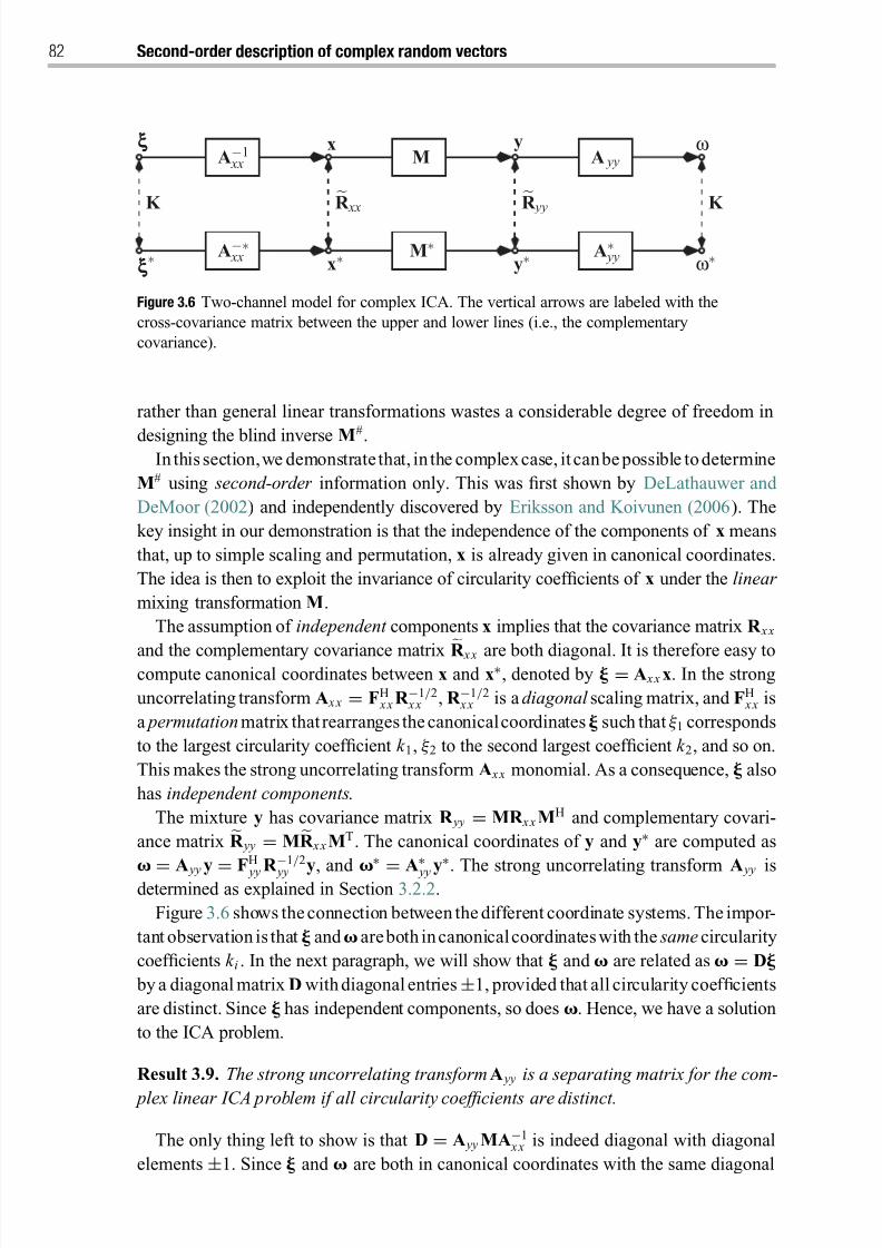
8/21/2019 Statistical Signal Processing of Complex-Valued Data.pdf
http://slidepdf.com/reader/full/statistical-signal-processing-of-complex-valued-datapdf 104/330
82 Second-order description of complex random vectors
ξξξ∗
K R yyR xxK
ω yxξξξAM yyA−1
xx
ω ∗A∗
yyy∗
M∗x∗
A−∗ xx
Figure 3.6 Two-channel model for complex ICA. The vertical arrows are labeled with the
cross-covariance matrix between the upper and lower lines (i.e., the complementary
covariance).
rather than general linear transformations wastes a considerable degree of freedom in
designing the blind inverse M#
.In this section,we demonstrate that, in the complexcase, it canbepossible to determine
M# using second-order information only. This was first shown by DeLathauwer and
DeMoor (2002) and independently discovered by Eriksson and Koivunen (2006). The
key insight in our demonstration is that the independence of the components of x means
that, up to simple scaling and permutation, x is already given in canonical coordinates.
The idea is then to exploit the invariance of circularity coefficients of x under the linear
mixing transformation M.
The assumption of independent components x implies that the covariance matrix R x x
and the complementary covariance matrix R x x are both diagonal. It is therefore easy tocompute canonical coordinates between x and x∗, denoted by = A x x x. In the strong
uncorrelating transform A x x = FH x x R −1/2
x x , R −1/2 x x is a diagonal scaling matrix, and FH
x x is
a permutation matrix that rearranges thecanonicalcoordinates such that ξ 1 corresponds
to the largest circularity coefficient k 1, ξ 2 to the second largest coefficient k 2, and so on.
This makes the strong uncorrelating transform A x x monomial. As a consequence, also
has independent components.
The mixture y has covariance matrix R yy = MR x x MH and complementary covari-
ance matrix
R yy = M
R x x MT. The canonical coordinates of y and y∗ are computed as
=
A yy
y=
FH
yyR −
1/2
yy y
, and
∗ =A∗ yy
y∗. The strong uncorrelating transform
A yy isdetermined as explained in Section 3.2.2.
Figure 3.6 shows theconnection between the different coordinate systems. The impor-
tant observation is that and areboth incanonicalcoordinateswith the same circularity
coefficients k i . In the next paragraph, we will show that and are related as = D
by a diagonal matrix D with diagonal entries±1, provided that all circularity coefficients
are distinct. Since has independent components, so does . Hence, we have a solution
to the ICA problem.
Result 3.9. The strong uncorrelating transform A yy is a separating matrix for the com-
plex linear ICA problem if all circularity coefficients are distinct.
The only thing left to show is that D = A yy MA−1 x x is indeed diagonal with diagonal
elements ±1. Since and are both in canonical coordinates with the same diagonal
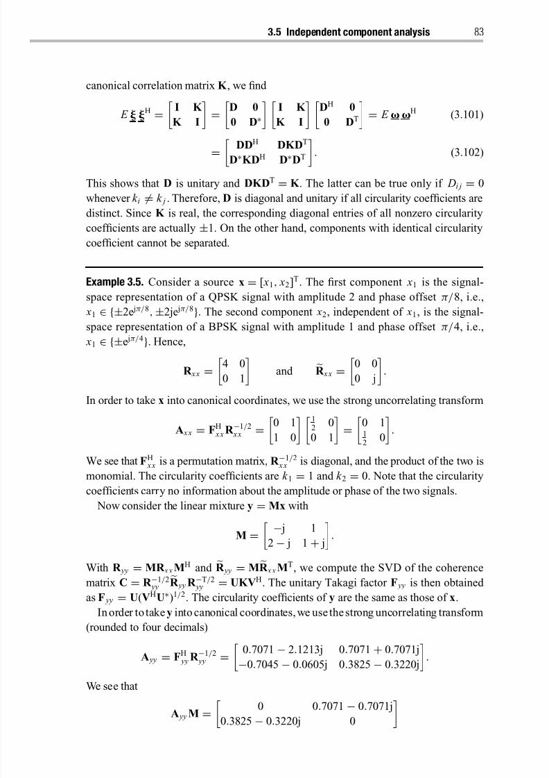
8/21/2019 Statistical Signal Processing of Complex-Valued Data.pdf
http://slidepdf.com/reader/full/statistical-signal-processing-of-complex-valued-datapdf 105/330
3.5 Independent component analysis 83
canonical correlation matrix K , we find
E H =
I K
K I
=
D 0
0 D∗
I K
K I
DH 0
0 DT
= E H (3.101)
= DDH DKDT
D∗KDH D∗DT
. (3.102)
This shows that D is unitary and DKDT = K . The latter can be true only if Di j = 0
whenever k i = k j . Therefore, D is diagonal and unitary if all circularity coefficients are
distinct. Since K is real, the corresponding diagonal entries of all nonzero circularity
coefficients are actually ±1. On the other hand, components with identical circularity
coefficient cannot be separated.
Example 3.5. Consider a source x = [ x1, x2]T. The first component x1 is the signal-
space representation of a QPSK signal with amplitude 2 and phase offset π/8, i.e.,
x1 ∈ {±2e jπ/8,±2je jπ/8}. The second component x2, independent of x1, is the signal-
space representation of a BPSK signal with amplitude 1 and phase offset π/4, i.e.,
x1 ∈ {±e jπ/4}. Hence,
R x x =
4 0
0 1
and R x x =
0 0
0 j
.
In order to take x into canonical coordinates, we use the strong uncorrelating transform
A x x = FH x x R −1/2
x x =
0 1
1 0
12
0
0 1
=
0 112
0
.
We see that FH x x is a permutation matrix, R −1/2
x x is diagonal, and the product of the two is
monomial. The circularity coefficients are k 1 = 1 and k 2 = 0. Note that the circularity
coefficients carry no information about the amplitude or phase of the two signals.
Now consider the linear mixture y = Mx with
M
= − j 1
2 − j 1 + j.
With R yy = MR x x MH and R yy = MR x x MT, we compute the SVD of the coherence
matrix C = R −1/2 yy
R yy R −T/2 yy = UKVH. The unitary Takagi factor F yy is then obtained
as F yy = U(VHU∗)1/2. The circularity coefficients of y are the same as those of x.
In order to take y into canonical coordinates, we use thestrong uncorrelating transform
(rounded to four decimals)
A yy = FH yy R −1/2
yy =
0.7071 − 2.1213j 0.7071 + 0.7071j
−0.7045 − 0.0605j 0.3825 − 0.3220j
.
We see that
A yy M =
0 0.7071 − 0.7071j
0.3825 − 0.3220j 0
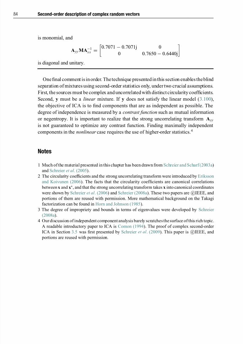
8/21/2019 Statistical Signal Processing of Complex-Valued Data.pdf
http://slidepdf.com/reader/full/statistical-signal-processing-of-complex-valued-datapdf 106/330
84 Second-order description of complex random vectors
is monomial, and
A yy MA−1 x x =
0.7071 − 0.7071j 0
0 0.7650 − 0.6440j
is diagonal and unitary.
Onefinal comment is in order. Thetechnique presented in this section enables theblind
separation of mixtures using second-order statistics only, under two crucial assumptions.
First, the sources must be complex and uncorrelated with distinct circularity coefficients.
Second, y must be a linear mixture. If y does not satisfy the linear model (3.100),
the objective of ICA is to find components that are as independent as possible. The
degree of independence is measured by a contrast function such as mutual information
or negentropy. It is important to realize that the strong uncorrelating transform A yyis not guaranteed to optimize any contrast function. Finding maximally independent
components in the nonlinear case requires the use of higher-order statistics.4
Notes
1 Much of the material presented in this chapter has been drawn from Schreier and Scharf (2003a)
and Schreier et al . (2005).
2 The circularity coefficients and the strong uncorrelating transform were introduced by Eriksson
and Koivunen (2006). The facts that the circularity coefficients are canonical correlations between x and x∗, and that the strong uncorrelating transfor m takes x into canonical coordinates
were shown by Schreier et al . (2006) and Schreier (2008a). These two papers are cIEEE, and
portions of them are reused with permission. More mathematical background on the Takagi
factorization can be found in Horn and Johnson (1985).
3 The degree of impropriety and bounds in terms of eigenvalues were developed by Schreier
(2008a).
4 Ourdiscussion of independent componentanalysisbarely scratches thesurface of this rich topic.
A readable introductory paper to ICA is Comon (1994). The pr oof of complex second-order
ICA in Section 3.5 was first presented by Schreier et al . (2009). This paper is cIEEE, and
portions are reused with permission.
8/21/2019 Statistical Signal Processing of Complex-Valued Data.pdf
http://slidepdf.com/reader/full/statistical-signal-processing-of-complex-valued-datapdf 107/330
4 Correlation analysis
Assessing multivariate association between two random vectors x and y is an important
problem in many research areas, ranging from the natural sciences (e.g., oceanography
and geophysics) to the social sciences (in particular psychometrics and behaviormet-
rics) and to engineering. While “multivariate association” is often simply visualized as
“similarity” between two random vectors, there are many different ways of measuring
it. In this chapter, we provide a unifying treatment of three popular correlation analysis
techniques: canonical correlation analysis (CCA), multivariate linear regression (MLR),
and partial least squares (PLS).1 Each of these techniques transforms x and y into its
respective internal representation and . Different correlation coefficients may then
be defined as functions of the diagonal cross-correlations {k i} between the internal
representations ξ i and ωi .
The key differences among CCA, MLR, and PLS are revealed in their invariance
properties. CCA is invariant under nonsingular linear transformation of x and y, MLR is
invariant under nonsingular linear transformation of y but only unitary transformation of
x, and PLS is invariant under unitary transformation of x and y. Correlation coefficients
then share the invariance properties of the correlation analysis technique on which they
are based.
Analyzing multivariate association of complex data is further complicated by the
fact that there are different types of correlation.2 Two scalar complex random variables
x and y are called rotationally dependent if x = ky for some complex constant k .
This term is motivated by the observation that, in the complex plane, sample pairs
of x and y rotate in the same direction (counterclockwise or clockwise), by the sameangle. They are called reflectionally dependent if x = k y∗ for some complex constant
k . This means that sample pairs of x and y rotate by the same angle, but in opposite
directions – one rotating clockwise and the other counterclockwise. Rotational and
reflectional correlations measure the degree of rotational and reflectional dependence.
The combined effect of rotational and reflectional correlation is assessed by a total
correlation.
Thus, there are two fundamental choices that must be made when analyzing multivari-
ate association between two complex random vectors: the desired invariance properties
of the analysis (linear/linear, unitary/linear, or unitary/unitary) and the type of correla-tion (rotational, reflectional, or total). These choices will have to be motivated by the
problem under consideration.
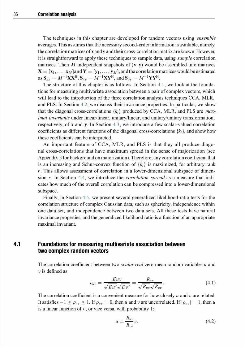
8/21/2019 Statistical Signal Processing of Complex-Valued Data.pdf
http://slidepdf.com/reader/full/statistical-signal-processing-of-complex-valued-datapdf 108/330
86 Correlation analysis
The techniques in this chapter are developed for random vectors using ensemble
averages. This assumes that the necessary second-order information is available, namely,
the correlationmatricesof x and y and their cross-correlation matrix areknown.However,
it is straightforward to apply these techniques to sample data, using sample correlation
matrices. Then M independent snapshots of (x, y) would be assembled into matrices
X = [x1, . . . , x M ]and Y = [y1, . . . , y M ], andthe correlation matrices would be estimated
as S x x = M −1XXH, S x y = M −1XYH, and S yy = M −1YYH.
The structure of this chapter is as follows. In Section 4.1, we look at the founda-
tions for measuring multivariate association between a pair of complex vectors, which
will lead to the introduction of the three correlation analysis techniques CCA, MLR,
and PLS. In Section 4.2, we discuss their invariance properties. In particular, we show
that the diagonal cross-correlations {k i} produced by CCA, MLR, and PLS are max-
imal invariants under linear/linear, unitary/linear, and unitary/unitary transformation,
respectively, of x and y. In Section 4.3, we introduce a few scalar-valued correlation
coefficients as different functions of the diagonal cross-correlations {k i }, and show how
these coefficients can be interpreted.
An important feature of CCA, MLR, and PLS is that they all produce diago-
nal cross-correlations that have maximum spread in the sense of majorization (see
Appendix 3 for background on majorization). Therefore, any correlation coefficient that
is an increasing and Schur-convex function of {k i } is maximized, for arbitrary rank
r . This allows assessment of correlation in a lower-dimensional subspace of dimen-
sion r . In Section 4.4, we introduce the correlation spread as a measure that indi-
cates how much of the overall correlation can be compressed into a lower-dimensional
subspace.
Finally, in Section 4.5, we present several generalized likelihood-ratio tests for the
correlation structure of complex Gaussian data, such as sphericity, independence within
one data set, and independence between two data sets. All these tests have natural
invariance properties, and the generalized likelihood ratio is a function of an appropriate
maximal invariant.
4.1 Foundations for measuring multivariate association betweentwo complex random vectors
The correlation coefficient between two scalar real zero-mean random variables u and
v is defined as
ρuv = Euv√
Eu2√
E v2= Ruv√
Ruu
√ Rvv
. (4.1)
The correlation coefficient is a convenient measure for how closely u and v are related.
It satisfies −1 ≤ ρuv ≤ 1. If ρuv = 0, then u and v are uncorrelated. If |ρuv| = 1, then uis a linear function of v, or vice versa, with probability 1:
u = Ruv
Rvv
v. (4.2)
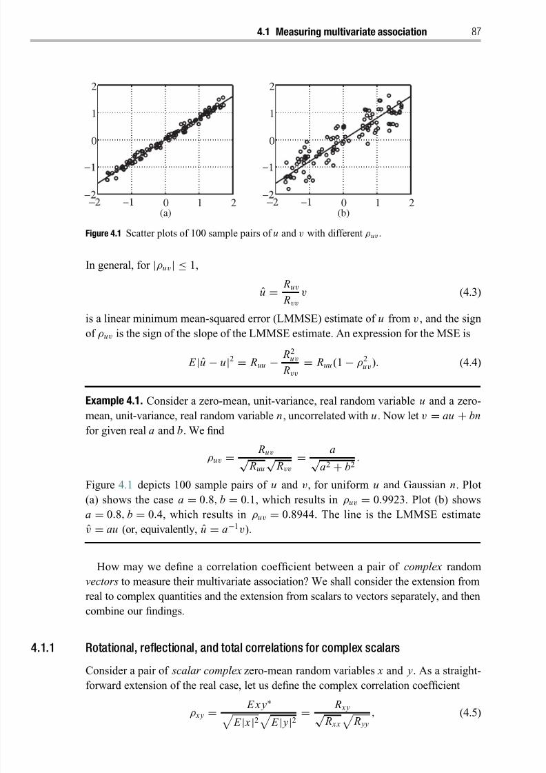
8/21/2019 Statistical Signal Processing of Complex-Valued Data.pdf
http://slidepdf.com/reader/full/statistical-signal-processing-of-complex-valued-datapdf 109/330
4.1 Measuring multivariate association 87
0 1 2
0
1
2
(b)0 1 2
0
1
2
(a)
Figure 4.1 Scatter plots of 100 sample pairs of u and v with different ρuv .
In general, for |ρuv| ≤ 1,
u = Ruv
Rvv
v (4.3)
is a linear minimum mean-squared error (LMMSE) estimate of u from v , and the sign
of ρuv is the sign of the slope of the LMMSE estimate. An expression for the MSE is
E |u − u|2 = Ruu − R2
uv
Rvv
= Ruu (1 − ρ2uv). (4.4)
Example 4.1. Consider a zero-mean, unit-variance, real random variable u and a zero-mean, unit-variance, real random variable n , uncorrelated with u . Now let v = au + bn
for given real a and b. We find
ρuv = Ruv√
Ruu
√ Rvv
= a√ a2 + b2
.
Figure 4.1 depicts 100 sample pairs of u and v, for uniform u and Gaussian n. Plot
(a) shows the case a = 0.8, b = 0.1, which results in ρuv = 0.9923. Plot (b) shows
a = 0.8, b = 0.4, which results in ρuv = 0.8944. The line is the LMMSE estimate
v
=au (or, equivalently, u
=a−1v).
How may we define a correlation coefficient between a pair of complex random
vectors to measure their multivariate association? We shall consider the extension from
real to complex quantities and the extension from scalars to vectors separately, and then
combine our findings.
4.1.1 Rotational, reflectional, and total correlations for complex scalars
Consider a pair of scalar complex zero-mean random variables x and y. As a straight-
forward extension of the real case, let us define the complex correlation coefficient
ρ x y = E x y∗
E | x |2
E | y|2= R x y√
R x x
R yy
, (4.5)
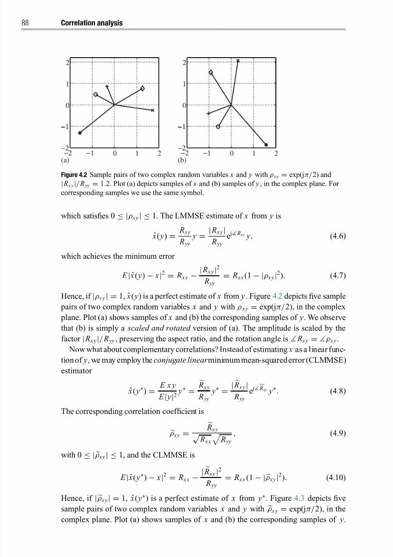
8/21/2019 Statistical Signal Processing of Complex-Valued Data.pdf
http://slidepdf.com/reader/full/statistical-signal-processing-of-complex-valued-datapdf 110/330
88 Correlation analysis
0 1 2
0
1
2
(a)0 1 2
0
1
2
(b)
Figure 4.2 Sample pairs of two complex random variables x and y with ρ x y = exp(jπ/2) and
| R x y |/ R yy = 1.2. Plot (a) depicts samples of x and (b) samples of y , in the complex plane. For
corresponding samples we use the same symbol.
which satisfies 0 ≤ |ρ x y| ≤ 1. The LMMSE estimate of x from y is
ˆ x( y) = R x y
R yy
y = | R x y | R yy
e j R xy y, (4.6)
which achieves the minimum error
E | ˆ x( y) − x|2 = R x x −| R x y|2
R yy
= R x x (1 − |ρ x y|2). (4.7)
Hence, if |ρ x y | = 1, ˆ x( y) is a perfect estimate of x from y . Figure 4.2 depicts five sample
pairs of two complex random variables x and y with ρ x y = exp(jπ/2), in the complex
plane. Plot (a) shows samples of x and (b) the corresponding samples of y. We observe
that (b) is simply a scaled and rotated version of (a). The amplitude is scaled by the
factor | R x y|/ R yy , preserving the aspect ratio, and the rotation angle is R x y = ρ x y .
Now what about complementary correlations? Instead of estimating x as a linear func-
tion of y, we may employ the conjugate linear minimummean-squarederror (CLMMSE)
estimator
ˆ x( y∗) = E x y
E | y|2 y∗ = R x y
R yy y∗ = | R x y
| R yye j R xy y∗. (4.8)
The corresponding correlation coefficient is
ρ x y = R x y√
R x x
R yy
, (4.9)
with 0 ≤ |ρ x y| ≤ 1, and the CLMMSE is
E | ˆ x( y∗) − x|2 = R x x −|
R x y |2 R
yy
= R x x (1 − |ρ x y |2). (4.10)
Hence, if |ρ x y| = 1, ˆ x( y∗) is a perfect estimate of x from y∗. Figure 4.3 depicts five
sample pairs of two complex random variables x and y with ρ x y = exp(jπ/2), in the
complex plane. Plot (a) shows samples of x and (b) the corresponding samples of y.
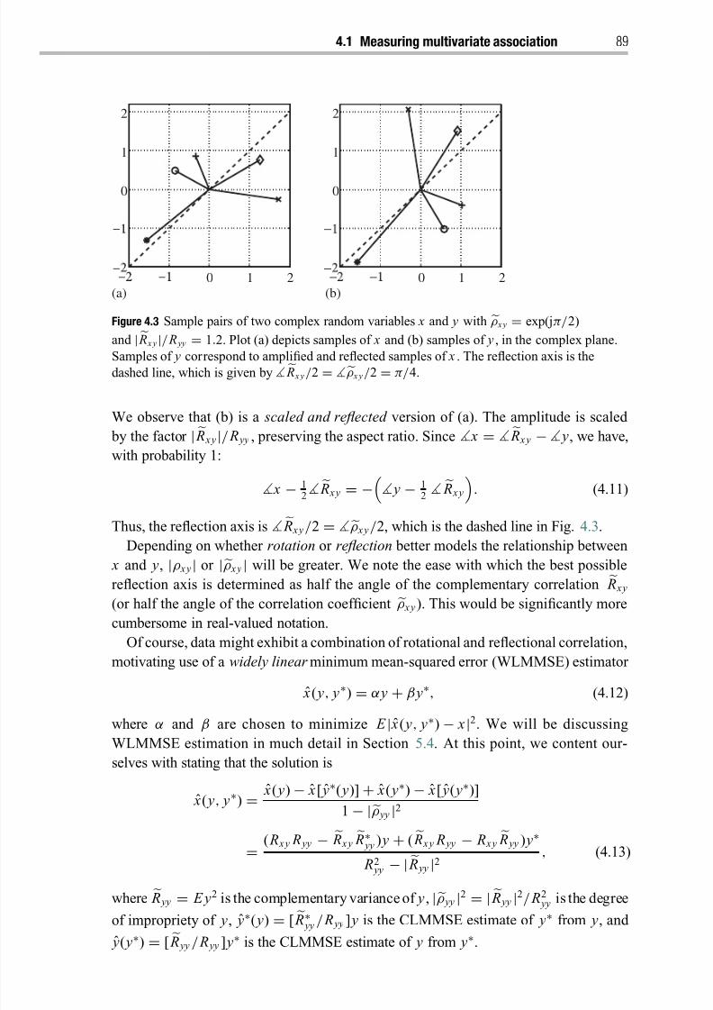
8/21/2019 Statistical Signal Processing of Complex-Valued Data.pdf
http://slidepdf.com/reader/full/statistical-signal-processing-of-complex-valued-datapdf 111/330
4.1 Measuring multivariate association 89
0 1 2
0
1
2
(a)
0 1 2
0
1
2
(b)
Figure 4.3 Sample pairs of two complex random variables x and y with
ρ x y = exp(jπ/2)
and
| R x y
|/ R yy
=1.2. Plot (a) depicts samples of x and (b) samples of y , in the complex plane.
Samples of y correspond to amplified and reflected samples of x . The reflection axis is thedashed line, which is given by R x y /2 = ρ x y /2 = π/4.
We observe that (b) is a scaled and reflected version of (a). The amplitude is scaled
by the factor | R x y|/ R yy , preserving the aspect ratio. Since x = R x y − y, we have,
with probability 1:
x − 12
R x y = −
y − 1
2
R x y
. (4.11)
Thus, the reflection axis is R x y /2 = ρ x y /2, which is the dashed line in Fig. 4.3.Depending on whether rotation or reflection better models the relationship between
x and y, |ρ x y| or |ρ x y | will be greater. We note the ease with which the best possible
reflection axis is determined as half the angle of the complementary correlation R x y
(or half the angle of the correlation coefficient ρ x y). This would be significantly more
cumbersome in real-valued notation.
Of course, data might exhibit a combination of rotational and reflectional correlation,
motivating use of a widely linear minimum mean-squared error (WLMMSE) estimator
ˆ x( y, y∗)
=α y
+β y∗, (4.12)
where α and β are chosen to minimize E | ˆ x( y, y∗) − x |2. We will be discussing
WLMMSE estimation in much detail in Section 5.4. At this point, we content our-
selves with stating that the solution is
ˆ x( y, y∗) = ˆ x( y) − ˆ x[ ˆ y∗( y)] + ˆ x( y∗) − ˆ x[ ˆ y( y∗)]
1 − |ρ yy |2
= ( R x y R yy −
R x y
R∗
yy ) y + (
R x y R yy − R x y
R yy ) y∗
R2 yy − | R yy |2
, (4.13)
where R yy = E y2 is the complementary variance of y , |ρ yy |2 = | R yy |2/ R2 yy is the degree
of impropriety of y, ˆ y∗( y) = [ R∗ yy / R yy ] y is the CLMMSE estimate of y∗ from y, and
ˆ y( y∗) = [ R yy / R yy ] y∗ is the CLMMSE estimate of y from y∗.
8/21/2019 Statistical Signal Processing of Complex-Valued Data.pdf
http://slidepdf.com/reader/full/statistical-signal-processing-of-complex-valued-datapdf 112/330
90 Correlation analysis
Through the connection
E | ˆ x( y, y∗) − x |2 = R x x (1 − ρ2 x y), (4.14)
we obtain the corresponding squared correlation coefficient
ρ2 x y =
|ρ x y |2 + |ρ x y|2 − 2 Re[ρ x y ρ∗ x y ρ yy ]
1 − |ρ yy |2
= (| R x y|2 + | R x y|2) R yy − 2 Re( R x y R∗
x y R yy )
R x x ( R2 yy − | R yy |2)
, (4.15)
with 0 ≤ ρ2 x y ≤ 1. We note that the correlation coefficient ρ x y , unlike ρ x y = ρ∗
yx and
ρ x y =
ρ yx , is not symmetric in x and y: in general, ρ2
x y = ρ2 yx .
The correlation coefficient ρ x y
is bounded in terms of the coefficients ρ x y
and ρ x y as
max(|ρ x y|2, |ρ x y |2) ≤ ρ2 x y ≤ min(|ρ x y|2 + |ρ x y |2, 1). (4.16)
The lower bound holds because a WLMMSE estimator subsumes both the LMMSE
and CLMMSE estimators, so we must have WLMMSE ≤ LMMSE and WLMMSE ≤CLMMSE. However, there is no general ordering of LMMSE and CLMMSE, which we
write as LMMSE CLMMSE.
A common scenario in which the lower bound is attained is when y is maximally
improper, i.e., R yy = |
R yy | ⇔ |
ρ yy |2 = 1, which yields a zero denominator in (4.15).
This means that, with probability 1, y∗ =
e jα y for some constant α, and R x y
=e jα R x y .
In this case, y and y∗ carry exactly the same information about x . Therefore, WLMMSE
estimation is unnecessary, and can be replaced with either LMMSE or CLMMSE esti-
mation. In the maximally improper case, ρ2 x y = |ρ x y |2 = |ρ x y |2. Two other examples
of attaining the lower bound in (4.16) are either R x y = 0 and R yy = 0 (i.e., ρ x y = 0
and ρ yy = 0), which leads to ρ2 x y = |ρ x y|2, or R x y = 0 and R yy = 0 (i.e., ρ x y = 0 and ρ yy = 0), which yields ρ2
x y = |ρ x y |2; cf. (4.15).
The upper bound ρ2 x y = |ρ x y |2 + |ρ x y|2 is attained when the WLMMSE estimator is
the sum of the LMMSE and CLMMSE estimators: ˆ x( y, y∗) = ˆ x( y) + ˆ x( y∗). In this case,
y and y∗ carry completely complementary information about x . This is possible only for
uncorrelated y and y∗, that is, a proper y. It is easy to see that R yy = 0 ⇔ |ρ yy |2 = 0
in (4.15) leads to ρ2 x y = |ρ x y |2 + |ρ x y|2. The following example gives two scenarios in
which the lower and upper bounds are attained.
Example 4.2. Attaining the lower bound . Consider a complex random variable
y = e jα(u + n),
where u is a real random variable and α is a fixed constant. Further, assume that n
is a real random variable, uncorrelated with u, and Rnn = Ruu . Let x = Re(e jαu) =cos(α)u. The LMMSE estimator ˆ x( y) = 1
2 cos(α)e− jα y and the CLMMSE estimator
ˆ x( y∗) = 12 cos(α)e jα y∗ both perform equally well. However, they both extract the same
information from y because y is maximally improper. Hence, a WLMMSE estimator has

8/21/2019 Statistical Signal Processing of Complex-Valued Data.pdf
http://slidepdf.com/reader/full/statistical-signal-processing-of-complex-valued-datapdf 113/330
4.1 Measuring multivariate association 91
no performance advantage over an LMMSE or CLMMSE estimator: |ρ x y|2 = |ρ x y|2 =ρ2
x y = 12.
Attaining the upper bound. Consider a proper complex random variable y and let
x be its real part. The LMMSE estimator of x from y is ˆ x( y) = 1
2 y, the CLMMSEestimator is ˆ x( y∗) = 12 y∗, and the WLMMSE estimator ˆ x( y, y∗) = 1
2 y + 1
2 y∗ produces
a perfect estimate of x . Here, rotational and reflectional models are equally appropriate.
Each tells only half the story, but they complement each other perfectly. It is easy
to see that |ρ x y |2 = |ρ x y |2 = 12 and ρ2
x y = |ρ x y|2 + |ρ x y |2 = 1. (This also shows that
ρ2 x y = ρ2
yx since it is obviously impossible to perfectly reconstruct y as a widely linear
function of x .)
The following definition sums up the main findings of this section, and will be used
to classify correlation coefficients throughout this chapter.
Definition 4.1. A correlation coefficient that measures how well a
(1) linear function
(2) conjugate linear function
(3) widely linear function
models the relationship between two complex random variables is respectively called a
(1) rotational correlation coefficient
(2) reflectional correlation coefficient (3) total correlation coefficient.
4.1.2 Principle of multivariate correlation analysis
We would now like to define a scalar-valued correlation coefficient that gives an overall
measure of the association between two zero-mean random vectors. The following
definition sets out the minimum requirements for such a correlation coefficient.
Definition 4.2. A correlation coefficient ρ x y between two random vectors x and y must satisfy the following conditions for all nonzero scalars α and β , provided that x and y
are not both zero.
0 ≤ ρ x y ≤ 1, (4.17)
ρ x y = ρ x y = ρ x y for x = αx, y = βy, (4.18)
ρ x y = 1 if y = βx, (4.19)
ρ x y = 0 if x and y are uncorrelated . (4.20)
Note that we do not require the symmetry ρ x y = ρ yx .3 If a correlation coefficient isallowed to be negative or complex-valued (as we have seen in the previous section),
these conditions apply to its absolute value. However, the correlation coefficients con-
sidered hereafter are all real and nonnegative. For simplicity, we consider only rotational
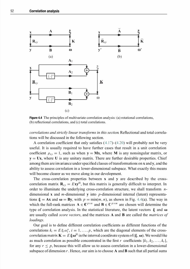
8/21/2019 Statistical Signal Processing of Complex-Valued Data.pdf
http://slidepdf.com/reader/full/statistical-signal-processing-of-complex-valued-datapdf 114/330
92 Correlation analysis
(a) (b)
(c)
R xy
B2
B1
A2
A1
ω
ξ
ξξξ
ω ω ∗ωω B
K
A
K
A
B
(·)∗
(·)∗
K
x
y
x
y
x
y∗
ξξξ
R xyR xy
Figure 4.4 The principles of multivariate correlation analysis: (a) rotational correlations,
(b) reflectional correlations, and (c) total correlations.
correlations and strictly linear transforms in this section. Reflectional and total correla-
tions will be discussed in the following section.
A correlation coefficient that only satisfies (4.17) –(4.20) will probably not be very
useful. It is usually required to have further cases that result in a unit correlation
coefficient ρ x y = 1, such as when y = Mx, where M is any nonsingular matrix, or
y = Ux, where U is any unitary matrix. There are further desirable properties. Chief
among them are invariance under specified classes of transformations on x and y, and the
ability to assess correlation in a lower-dimensional subspace. What exactly this means
will become clearer as we move along in our development.
The cross-correlation properties between x and y are described by the cross-
correlation matrix R x y
= E xyH, but this matrix is generally difficult to interpret. In
order to illuminate the underlying cross-correlation structure, we shall transform n-dimensional x and m-dimensional y into p-dimensional internal (latent) representa-
tions = Ax and = By, with p = min(m, n), as shown in Fig. 4.4(a). The way in
which the full-rank matrices A ∈ C p×n and B ∈ C p×m are chosen will determine the
type of correlation analysis. In the statistical literature, the latent vectors and
are usually called score vectors, and the matrices A and B are called the matrices of
loadings.
Our goal is to define different correlation coefficients as different functions of the
correlations k i = E ξ i ω∗i , i = 1, . . . , p , which are the diagonal elements of the cross-
correlation matrix K = E H in the internal coordinate system of (, ). We would likeas much correlation as possible concentrated in the first r coefficients {k 1, k 2, . . . , k r },for any r ≤ p, because this will allow us to assess correlation in a lower-dimensional
subspace of dimension r . Hence, our aim is to choose A and B such that all partial sums
8/21/2019 Statistical Signal Processing of Complex-Valued Data.pdf
http://slidepdf.com/reader/full/statistical-signal-processing-of-complex-valued-datapdf 115/330
4.1 Measuring multivariate association 93
over the absolute values of the diagonal cross-correlations k i are maximized:
maxA,B
r
i=1
|k i |, r = 1, . . . , p (4.21)
In order to make this a well-defined maximization problem, we need to impose some
constraints on A and B. The following three choices are most compelling.
Require that the internal representations and each have identity correlation matrix
(we avoid using the term “white” because and may have non-identity complemen-
tary correlation matrices): R ξ ξ = AR x x AH = I and R ωω = BR yy BH = I. This choice
leads to canonical correlation analysis (CCA). The corresponding diagonal cross-
correlations k i are called the canonical correlations, and the latent vectors and
are given in canonical coordinates.
Require that A have unitary rows (which we will simply call row-unitary) and haveidentity correlation matrix: AAH = I and R ωω = BR yy BH = I. This choice leads to
multivariate linear regression (MLR), also known as half-canonical correlation anal-
ysis. The corresponding diagonal cross-correlations k i are called the half-canonical
correlations, and the latent vectors and are given in half-canonical coordinates. Require that A and B be row-unitary: AAH = I and BBH = I. This choice leads to
partial least-squares (PLS) analysis. The corresponding diagonal cross-correlations
k i are called the PLS correlations, and the latent vectors and are given in PLS
coordinates.
Sometimes, when there is a risk of confusion, we will use the subscript C, M, or P to
emphasize that quantities were derived using CCA, MLR, or PLS.
Example 4.3. If x and y are scalars, then the CCA constraints are | A|2 = R−1 x x and | B|2 =
R−1 yy . Thus, the latent variables are ξ = R−1/2
x x e jφ1 x and ω = R−1/2 yy e jφ2 y for arbitrary φ1
and φ2. We then obtain
|k | = | E ξ ω∗| = | R x y |√ R x x R yy
= |ρ x y |,
with ρ x y defined in (4.5).
We will find in Section 4.1.4 that the solution to the maximization problem (4.21) for
CCA, MLR, or PLS results in a diagonal cross-correlation matrix
K = E H = Diag(k 1, . . . , k p), (4.22)
with k 1 ≥ k 2 ≥ · · · ≥ k p ≥ 0. Of course, the k i s depend on which of the principles
CCA, MLR, and PLS is employed, so they are canonical correlations, half-canonical
correlations, or PLS correlations. Furthermore, we will show that CCA, MLR, and PLSeach produce a set {k i} that has maximum spread in the sense of majorization (see
Appendix 3). Therefore, any correlation coefficient that is an increasing, Schur-convex
function of {k i } is maximized, for arbitrary rank r .
8/21/2019 Statistical Signal Processing of Complex-Valued Data.pdf
http://slidepdf.com/reader/full/statistical-signal-processing-of-complex-valued-datapdf 116/330
94 Correlation analysis
The key difference among CCA, MLR, and PLS lies in their invariance properties.
We will see that CCA is invariant under nonsingular linear transformation of both x
and y, MLR is invariant under nonsingular linear transformation of y but only unitary
transformation of x, and PLS is invariant under unitary transformation of both x and y.
Therefore, CCA and PLS provide a symmetric assessment of correlation since the roles
of x and y are interchangeable. MLR, on the other hand, distinguishes between the mes-
sage (or predictor/explanatory variables) x and the measurement (or criterion/response
variables) y. The correlation analysis technique must be chosen to match the invariance
properties of the problem at hand.
4.1.3 Rotational, reflectional, and total correlations for complex vectors
It is easy to see how to apply these principles to reflectional and total correlations, as
shown in Figs. 4.4( b) and (c). For reflectional correlations, the internal representation is
= Ax and ∗ = By∗, whose complementary cross-correlation matrix is K = E T,
and k i = E ξ i ωi . The maximization problem is then to maximize all partial sums over
the absolute value of the complementary cross-correlations
maxA,Br
i=1
|k i |, r = 1, . . . , p, (4.23)
with the following constraints on
A and
B.
For CCA, AR x x AH = I and BR ∗ yy BH = I. For MLR, AAH = I and BR ∗ yy
BH = I. For PLS, AAH = I and BBH = I.
For total correlations, the internal representation is computed as a widely linear
function: = A x (i.e., = A1x + A2x∗) and = B y (i.e., = B1y + B2y∗). Here,
our goal is to maximize the diagonal cross-correlations between the vectors of real and
imaginary parts of and . That is, for i = 1, . . . , p , we let
k 2i−
1
=2 E (Re ξ i Re ωi )
=Re( E ξ i ω∗
i + E ξ i ωi ), (4.24)
k 2i = 2 E (Im ξ i Im ωi ) = Re( E ξ i ω∗i − E ξ i ωi ), (4.25)
and maximize
maxA,B
r i=1
|k i |, r = 1, . . . , 2 p, (4.26)
with the following constraints placed on A and B.
For CCA, A R x x AH = I and B R yy BH = I. Hence, and are each white and
proper. For MLR, A AH = I and B R yy BH = I. While is white and proper, is generally
improper. For PLS, A AH = I and B BH = I. Both and are generally improper.
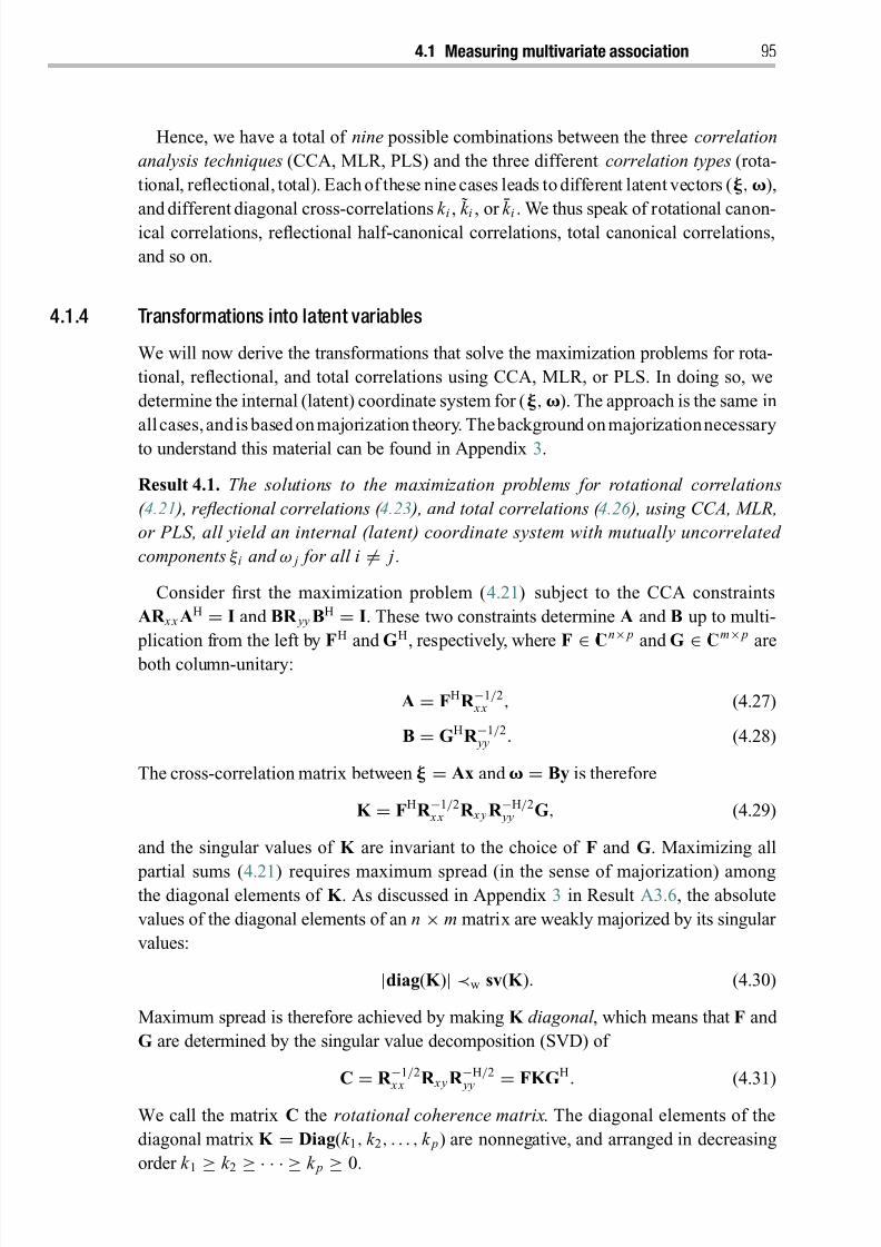
8/21/2019 Statistical Signal Processing of Complex-Valued Data.pdf
http://slidepdf.com/reader/full/statistical-signal-processing-of-complex-valued-datapdf 117/330
4.1 Measuring multivariate association 95
Hence, we have a total of nine possible combinations between the three correlation
analysis techniques (CCA, MLR, PLS) and the three different correlation types (rota-
tional, reflectional, total). Each of these nine cases leads to different latent vectors (, ),
and different diagonal cross-correlations k i, k
i, or k
i. We thus speak of rotational canon-
ical correlations, reflectional half-canonical correlations, total canonical correlations,
and so on.
4.1.4 Transformations into latent variables
We will now derive the transformations that solve the maximization problems for rota-
tional, reflectional, and total correlations using CCA, MLR, or PLS. In doing so, we
determine the internal (latent) coordinate system for (, ). The approach is the same in
allcases, andis based on majorization theory. Thebackground on majorizationnecessary
to understand this material can be found in Appendix 3.
Result 4.1. The solutions to the maximization problems for rotational correlations
( 4.21 ), reflectional correlations ( 4.23 ) , and total correlations ( 4.26 ) , using CCA, MLR,
or PLS, all yield an internal (latent) coordinate system with mutually uncorrelated
components ξ i and ω j for all i = j .
Consider first the maximization problem (4.21) subject to the CCA constraints
AR x x AH = I and BR yy BH = I. These two constraints determine A and B up to multi-
plication from the left by FH and GH, respectively, where F
∈Cn× p and G
∈Cm× p are
both column-unitary:
A = FHR −1/2 x x , (4.27)
B = GHR −1/2 yy . (4.28)
The cross-correlation matrix between = Ax and = By is therefore
K = FHR −1/2 x x R x y R −H/2
yy G, (4.29)
and the singular values of K are invariant to the choice of F and G. Maximizing all
partial sums (4.21) requires maximum spread (in the sense of majorization) amongthe diagonal elements of K . As discussed in Appendix 3 in Result A3.6, the absolute
values of the diagonal elements of an n × m matrix are weakly majorized by its singular
values:
|diag(K )| ≺w sv(K ). (4.30)
Maximum spread is therefore achieved by making K diagonal , which means that F and
G are determined by the singular value decomposition (SVD) of
C
=R −1/2
x x R x y R −H/2 yy
=FKGH. (4.31)
We call the matrix C the rotational coherence matrix. The diagonal elements of the
diagonal matrix K = Diag(k 1, k 2, . . . , k p) are nonnegative, and arranged in decreasing
order k 1 ≥ k 2 ≥ · · · ≥ k p ≥ 0.
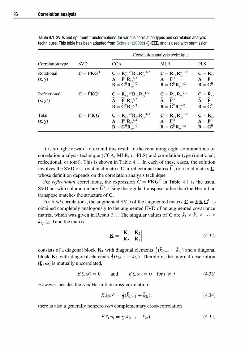
8/21/2019 Statistical Signal Processing of Complex-Valued Data.pdf
http://slidepdf.com/reader/full/statistical-signal-processing-of-complex-valued-datapdf 118/330
96 Correlation analysis
Table 4.1 SVDs and optimum transformations for various correlation types and correlation analysis
techniques. This table has been adapted from Schreier (2008c) cIEEE, and is used with permission.
Correlation analysis technique
Correlation type SVD CCA MLR PLS
Rotational C = FKGH C = R −1/2 x x R x y R −H/2
yy C = R x y R −H/2 yy C = R x y
(x, y) A = FHR −1/2 x x A = FH A = FH
B = GHR −1/2 yy B = GHR −1/2
yy B = GH
Reflectional C = FK GT C = R −1/2 x x R x y R −T/2
yyC = R x y R −T/2
yyC = R x y
(x, y∗) A = FHR −1/2 x x
A = FH A = FH
B =
GTR −∗/2
yy
B =
GTR −∗/2
yy
B =
GT
Total C = F K GH C = R −1/2 x x R x y R −H/2
yy C = R x y R −H/2 yy C = R x y
(x, y) A = FHR −1/2 x x A = FH A = FH
B = GHR −1/2 yy B = GHR −1/2
yy B = GH
It is straightforward to extend this result to the remaining eight combinations of
correlation analysis technique (CCA, MLR, or PLS) and correlation type (rotational,
reflectional, or total). This is shown in Table 4.1. In each of these cases, the solution
involves the SVD of a rotational matrix C, a reflectional matrix
C, or a total matrix C,
whose definition depends on the correlation analysis technique.
For reflectional correlations, the expression C = FK GT in Table 4.1 is the usualSVD but with column-unitary G∗. Using the regular transpose rather than the Hermitian
transpose matches the structure of C.
For total correlations, the augmented SVD of the augmented matrix C = F K GH is
obtained completely analogously to the augmented EVD of an augmented covariance
matrix, which was given in Result 3.1. The singular values of C are k 1 ≥ k 2 ≥ · · · ≥k 2 p ≥ 0 and the matrix
K = K 1 K 2
K 2 K 1 (4.32)
consists of a diagonal block K 1 with diagonal elements 12(k 2i−1 + k 2i ) and a diagonal
block K 2 with diagonal elements 12(k 2i−1 − k 2i ). Therefore, the internal description
(, ) is mutually uncorrelated,
E ξ i ω∗ j = 0 and E ξ i ω j = 0 for i = j . (4.33)
However, besides the real Hermitian cross-correlation
E ξ i ω∗i = 1
2(k 2i−1 + k 2i ), (4.34)
there is also a generally nonzero real complementary cross-correlation
E ξ i ωi = 12(k 2i−1 − k 2i ), (4.35)
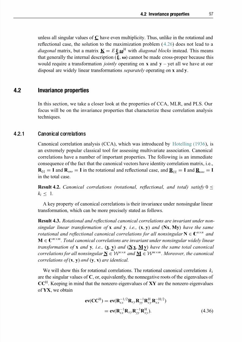
8/21/2019 Statistical Signal Processing of Complex-Valued Data.pdf
http://slidepdf.com/reader/full/statistical-signal-processing-of-complex-valued-datapdf 119/330
4.2 Invariance properties 97
unless all singular values of C have even multiplicity. Thus, unlike in the rotational and
reflectional case, the solution to the maximization problem (4.26) does not lead to a
diagonal matrix, but a matrix K = E H with diagonal blocks instead. This means
that generally the internal description (, ) cannot be made cross-proper because this
would require a transformation jointly operating on x and y – yet all we have at our
disposal are widely linear transformations separately operating on x and y.
4.2 Invariance properties
In this section, we take a closer look at the properties of CCA, MLR, and PLS. Our
focus will be on the invariance properties that characterize these correlation analysis
techniques.
4.2.1 Canonical correlations
Canonical correlation analysis (CCA), which was introduced by Hotelling (1936), is
an extremely popular classical tool for assessing multivariate association. Canonical
correlations have a number of important properties. The following is an immediate
consequence of the fact that the canonical vectors have identity correlation matrix, i.e.,
R ξ ξ = I and R ωω = I in the rotational and reflectional case, and R ξ ξ = I and R ωω = I
in the total case.
Result 4.2. Canonical correlations (rotational, reflectional, and total) satisfy 0 ≤k i ≤ 1.
A key property of canonical correlations is their invariance under nonsingular linear
transformation, which can be more precisely stated as follows.
Result 4.3. Rotational and reflectional canonical correlations are invariant under non-
singular linear transformation of x and y , i.e., (x, y) and (Nx, My) have the same
rotational and reflectional canonical correlations for all nonsingular N
∈Cn×n and
M ∈ Cm×m . Total canonical correlations are invariant under nonsingular widely linear transformation of x and y , i.e., (x, y) and (N x, M y) have the same total canonical
correlations for all nonsingular N ∈W n×n and M ∈W m×m . Moreover, the canonical
correlations of (x, y) and (y, x) are identical.
We will show this for rotational correlations. The rotational canonical correlations k i
are the singular values of C, or, equivalently, the nonnegative roots of the eigenvalues of
CCH. Keeping in mind that the nonzero eigenvalues of XY are the nonzero eigenvalues
of YX, we obtain
ev(CCH) = ev(R −1/2 x x R x y R −1 yy R H x y R −H/2 x x )
= ev(R −1 x x R x y R −1
yy R H x y). (4.36)
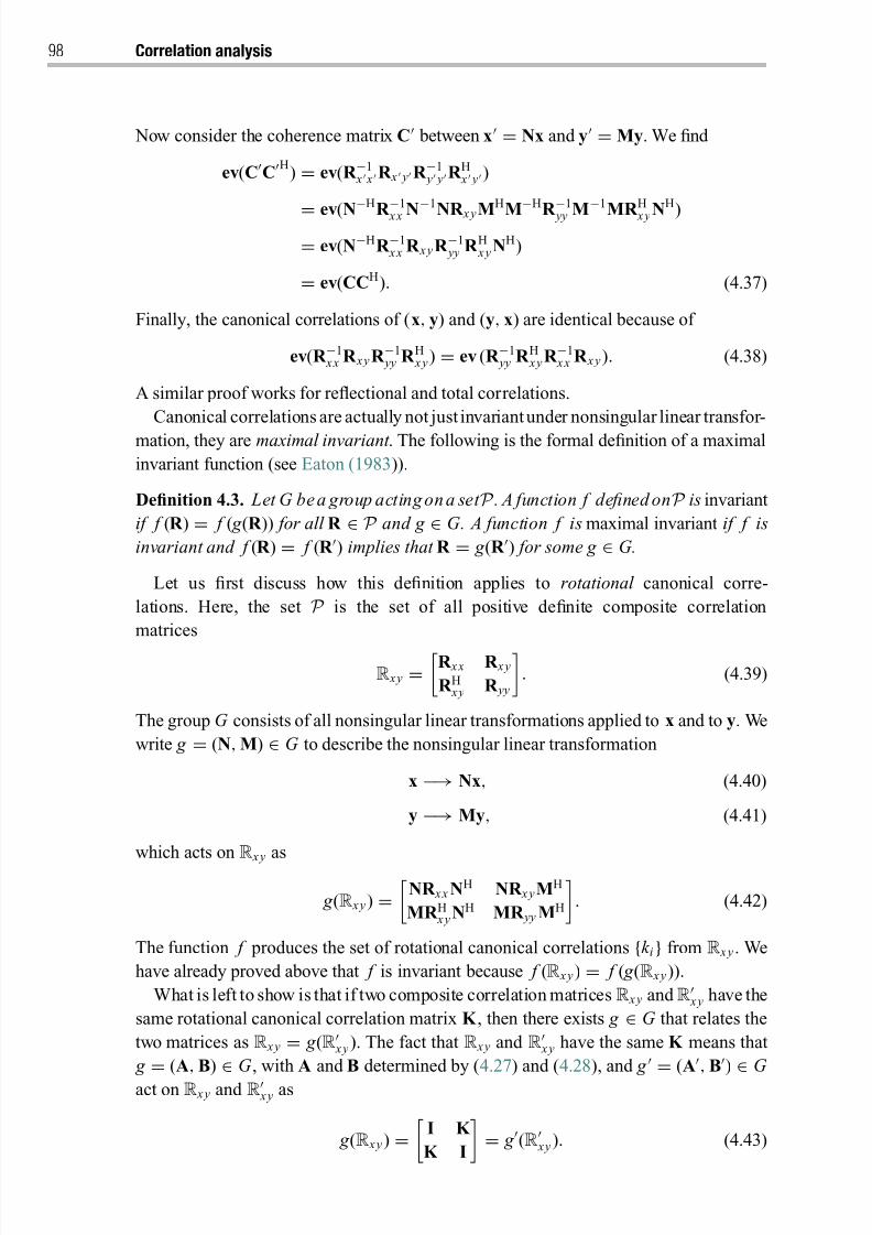
8/21/2019 Statistical Signal Processing of Complex-Valued Data.pdf
http://slidepdf.com/reader/full/statistical-signal-processing-of-complex-valued-datapdf 120/330
98 Correlation analysis
Now consider the coherence matrix C between x = Nx and y = My. We find
ev(CCH) = ev(R −1 x x R x yR −1
y yR H x y)
= ev(N−H
R −1
x x N−1
NR x y M
H
M−H
R −1
yy M−1
MR
H
x y N
H
)
= ev(N−HR −1 x x R x y R −1
yy R H x y NH)
= ev(CCH). (4.37)
Finally, the canonical correlations of (x, y) and (y, x) are identical because of
ev(R −1 x x R x y R −1
yy R H x y) = ev (R −1 yy R H x y R −1
x x R x y). (4.38)
A similar proof works for reflectional and total correlations.
Canonical correlations are actually not just invariantunder nonsingular linear transfor-
mation, they are maximal invariant . The following is the formal definition of a maximal
invariant function (see Eaton (1983)).
Definition 4.3. Let G be a group acting on a set P . A function f defined onP is invariant
if f (R ) = f ( g (R )) for all R ∈ P and g ∈ G. A function f is maximal invariant if f is
invariant and f (R ) = f (R ) implies that R = g (R ) for some g ∈ G.
Let us first discuss how this definition applies to rotational canonical corre-
lations. Here, the set P is the set of all positive definite composite correlation
matrices
R x y =R x x R x y
R H x y R yy
. (4.39)
The group G consists of all nonsingular linear transformations applied to x and to y. We
write g = (N, M) ∈ G to describe the nonsingular linear transformation
x −→ Nx, (4.40)
y −→ My, (4.41)
which acts on R x y as
g (R x y) =
NR x x NH NR x y MH
MR H x y NH MR yy MH
. (4.42)
The function f produces the set of rotational canonical correlations {k i} from R x y . We
have already proved above that f is invariant because f (R x y) = f ( g (R x y)).
What is left to show is that if two composite correlation matricesR x y and R x y have the
same rotational canonical correlation matrix K , then there exists g ∈ G that relates the
two matrices as R x y = g (R x y). The fact that R x y and R
x y have the same K means that
g
=(A, B)
∈G , with A and B determined by (4.27) and (4.28), and g
=(A, B)
∈G
act on R x y and R x y as
g (R x y) =
I K
K I
= g (R
x y). (4.43)
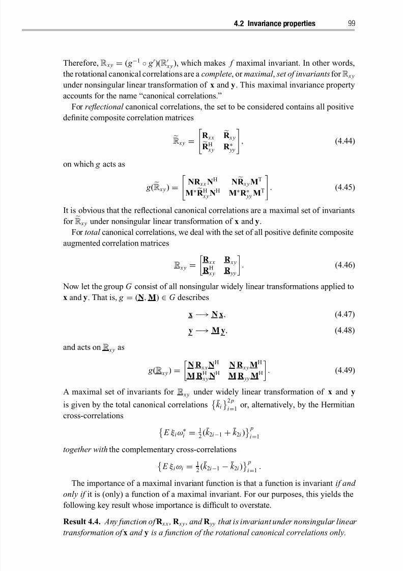
8/21/2019 Statistical Signal Processing of Complex-Valued Data.pdf
http://slidepdf.com/reader/full/statistical-signal-processing-of-complex-valued-datapdf 121/330
4.2 Invariance properties 99
Therefore, R x y = ( g −1 ◦ g )(R x y), which makes f maximal invariant. In other words,
the rotational canonical correlations are a complete, or maximal , set of invariants for R x y
under nonsingular linear transformation of x and y. This maximal invariance property
accounts for the name “canonical correlations.”For reflectional canonical correlations, the set to be considered contains all positive
definite composite correlation matrices
R x y =
R x x R x yR H x y R ∗ yy
, (4.44)
on which g acts as
g (
R x y) =
NR x x NH N
R x y MT
M∗R H x y NH M∗R ∗ yy MT. (4.45)
It is obvious that the reflectional canonical correlations are a maximal set of invariants
for R x y under nonsingular linear transformation of x and y.
For total canonical correlations, we deal with the set of all positive definite composite
augmented correlation matrices
R x y =
R x x R x y
R H x y R yy
. (4.46)
Now let the group G consist of all nonsingular widely linear transformations applied to
x and y. That is, g = (N, M) ∈ G describes
x −→ N x, (4.47)
y −→ M y, (4.48)
and acts on R x y as
g (R x y) =
N R x x NH N R x y MH
M R H x y NH M R yy MH
. (4.49)
A maximal set of invariants for R x y under widely linear transformation of x and y
is given by the total canonical correlations k i2 pi=1
or, alternatively, by the Hermitian
cross-correlations E ξ i ω∗
i = 12(k 2i−1 + k 2i )
p
i=1
together with the complementary cross-correlations E ξ i ωi = 1
2(k 2i−1 − k 2i )
p
i=1.
The importance of a maximal invariant function is that a function is invariant if and
only if it is (only) a function of a maximal invariant. For our purposes, this yields the
following key result whose importance is difficult to overstate.
Result 4.4. Any function of R x x , R x y , and R yy that is invariant under nonsingular linear
transformation of x and y is a function of the rotational canonical correlations only.
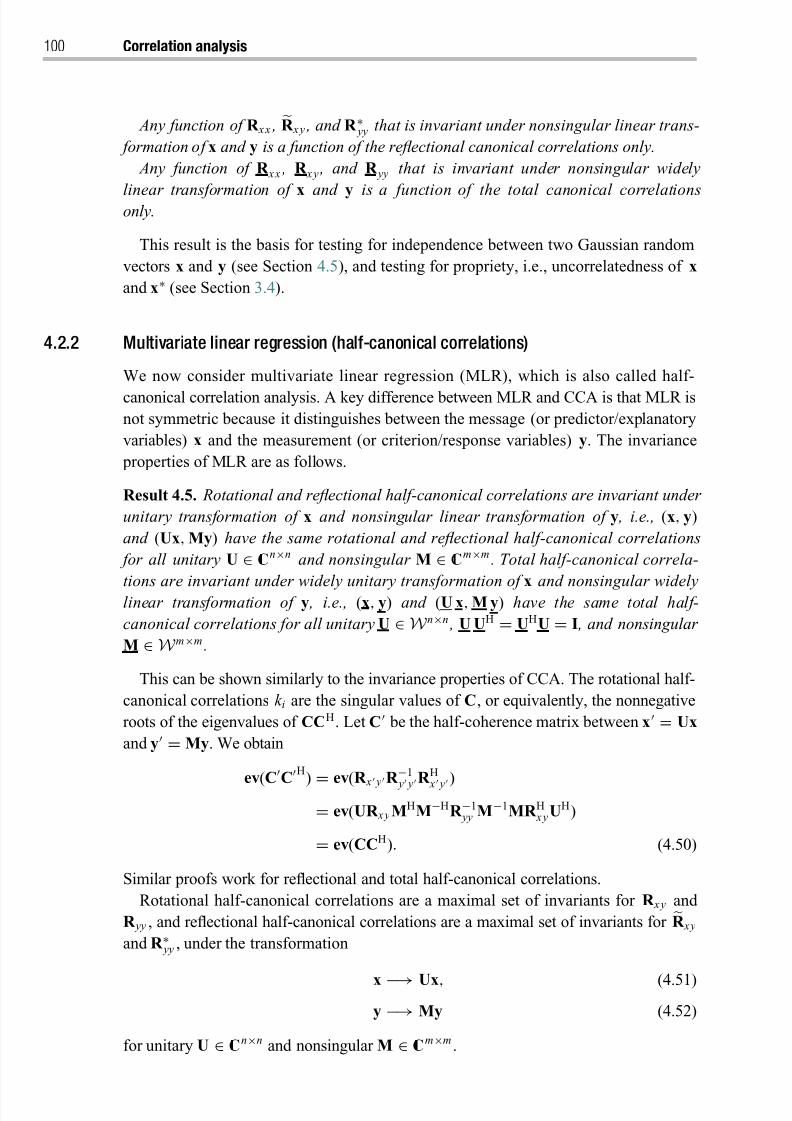
8/21/2019 Statistical Signal Processing of Complex-Valued Data.pdf
http://slidepdf.com/reader/full/statistical-signal-processing-of-complex-valued-datapdf 122/330
100 Correlation analysis
Any function of R x x , R x y , and R ∗ yy that is invariant under nonsingular linear trans-
formation of x and y is a function of the reflectional canonical correlations only.
Any function of R x x , R x y , and R yy that is invariant under nonsingular widely
linear transformation of x and y is a function of the total canonical correlationsonly.
This result is the basis for testing for independence between two Gaussian random
vectors x and y (see Section 4.5), and testing for propriety, i.e., uncorrelatedness of x
and x∗ (see Section 3.4).
4.2.2 Multivariate linear regression (half-canonical correlations)
We now consider multivariate linear regression (MLR), which is also called half-
canonical correlation analysis. A key difference between MLR and CCA is that MLR isnot symmetric because it distinguishes between the message (or predictor/explanatory
variables) x and the measurement (or criterion/response variables) y. The invariance
properties of MLR are as follows.
Result 4.5. Rotational and reflectional half-canonical correlations are invariant under
unitary transformation of x and nonsingular linear transformation of y , i.e., (x, y)
and (Ux, My) have the same rotational and reflectional half-canonical correlations
for all unitary U ∈ Cn×n and nonsingular M ∈ Cm×m . Total half-canonical correla-
tions are invariant under widely unitary transformation of x and nonsingular widelylinear transformation of y , i.e., (x, y) and (U x, M y) have the same total half-
canonical correlations for all unitary U ∈W n×n , U UH = UHU = I , and nonsingular
M ∈W m×m .
This can be shown similarly to the invariance properties of CCA. The rotational half-
canonical correlations k i are the singular values of C, or equivalently, the nonnegative
roots of the eigenvalues of CCH. Let C be the half-coherence matrix between x = Ux
and y = My. We obtain
ev(CCH
) = ev(R x yR −1
y yR
H
x y)= ev(UR x y MHM−HR −1
yy M−1MR H x y UH)
= ev(CCH). (4.50)
Similar proofs work for reflectional and total half-canonical correlations.
Rotational half-canonical correlations are a maximal set of invariants for R x y and
R yy , and reflectional half-canonical correlations are a maximal set of invariants for R x y
and R ∗ yy , under the transformation
x −→ Ux, (4.51)
y −→ My (4.52)
for unitary U ∈ Cn×n and nonsingular M ∈ Cm×m .

8/21/2019 Statistical Signal Processing of Complex-Valued Data.pdf
http://slidepdf.com/reader/full/statistical-signal-processing-of-complex-valued-datapdf 123/330
4.2 Invariance properties 101
Total half-canonical correlations are a maximal set of invariants for R x y and R yy
under the transformation
x
−→U x, (4.53)
y −→ M y (4.54)
for unitary U ∈W n×n and nonsingular M ∈W m×m . This maximal invariance property is
proved along the same lines as the maximal invariance property of canonical correlations
in the previous section. Thus, we have the following important result.
Result 4.6. Any function of R x y and R yy that is invariant under unitary transformation
of x and nonsingular linear transformation of y is a function of the rotational half-
canonical correlations only.
Any function of R x y and R ∗ yy that is invariant under unitary transformation of x and
nonsingular linear transformation of y is a function of the reflectional half-canonical
correlations only.
Any function of R x y and R yy that is invariant under widely unitary transformation
of x and nonsingular widely linear transformations of y is a function of the total half-
canonical correlations only.
One may have been tempted to assume that half-canonical correlations are maximal
invariants for the composite correlation matrices R x y in (4.39), R x y in (4.44), or R x y
in (4.46). But it is clear that half-canonical correlations do not characterize R x x or
R x x
. A maximal set of invariants for R x x
under unitary transformation of x is the set
of eigenvalues of R x x , and a maximal set of invariants for R x x under widely unitary
transformation of x is the set of eigenvalues of R x x . For instance, tr R x x , which is
invariant under unitary transformation, is the sum of the eigenvalues of R x x .
Weighted MLR
A generalizationof MLR replaces thecondition that A have unitary rows, AAH = I, with
AWAH = I, where W ∈ Cn×n is a Hermitian, positive definite weighting matrix. In the
rotational case, the optimum transformations and corresponding SVD are then given by
A = FH
W−1/2
, (4.55)
B = GHR −1/2 yy , (4.56)
C = W−1/2R x y R −H/2 yy = FKGH. (4.57)
Extensions to the reflectional and total case work analogously. The invariance properties
of weighted half-canonical correlations are different than those of half-canonical corre-
lations and depend on the choice of W. It is interesting to note that canonical correlations
are actually weighted half-canonical correlations with weighting matrix W = R x x .
4.2.3 Partial least squares
Finally, we turn to partial least squares (PLS). We emphasize that there are many variants
of PLS. Our description of PLS follows Sampson et al . (1989), which differs from the
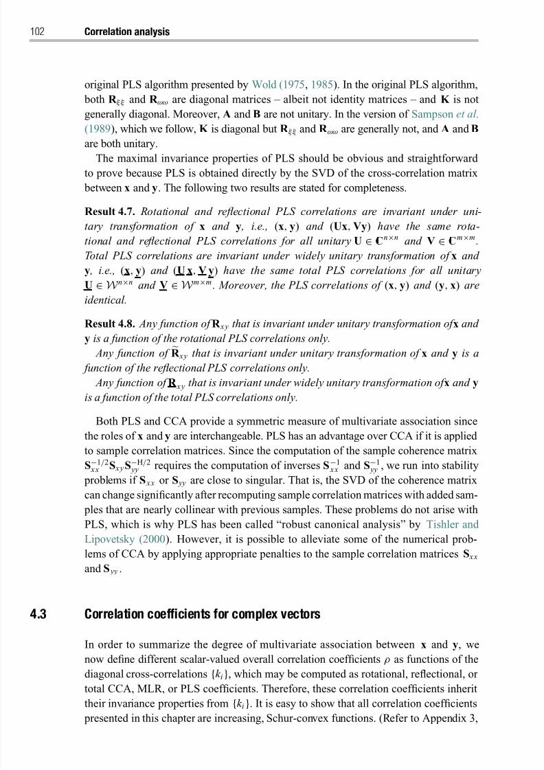
8/21/2019 Statistical Signal Processing of Complex-Valued Data.pdf
http://slidepdf.com/reader/full/statistical-signal-processing-of-complex-valued-datapdf 124/330
102 Correlation analysis
original PLS algorithm presented by Wold (1975, 1985). In the original PLS algorithm,
both R ξ ξ and R ωω are diagonal matrices – albeit not identity matrices – and K is not
generally diagonal. Moreover, A and B are not unitary. In the version of Sampson et al .
(1989), which we follow, K is diagonal but R ξ ξ
and R ωω
are generally not, and A and B
are both unitary.
The maximal invariance properties of PLS should be obvious and straightforward
to prove because PLS is obtained directly by the SVD of the cross-correlation matrix
between x and y. The following two results are stated for completeness.
Result 4.7. Rotational and reflectional PLS correlations are invariant under uni-
tary transformation of x and y , i.e., (x, y) and (Ux, Vy) have the same rota-
tional and reflectional PLS correlations for all unitary U ∈ Cn×n and V ∈ Cm×m .
Total PLS correlations are invariant under widely unitary transformation of x and
y , i.e., (x, y) and (U x, V y) have the same total PLS correlations for all unitaryU ∈W n×n and V ∈W m×m . Moreover, the PLS correlations of (x, y) and (y, x) are
identical.
Result 4.8. Any function of R x y that is invariant under unitary transformation of x and
y is a function of the rotational PLS correlations only.
Any function of R x y that is invariant under unitary transformation of x and y is a
function of the reflectional PLS correlations only.
Any function of R x y that is invariant under widely unitary transformation of x and y
is a function of the total PLS correlations only.
Both PLS and CCA provide a symmetric measure of multivariate association since
the roles of x and y are interchangeable. PLS has an advantage over CCA if it is applied
to sample correlation matrices. Since the computation of the sample coherence matrix
S−1/2 x x S x y S−H/2
yy requires the computation of inverses S−1 x x and S−1
yy , we run into stability
problems if S x x or S yy are close to singular. That is, the SVD of the coherence matrix
can change significantly after recomputing sample correlation matrices with added sam-
ples that are nearly collinear with previous samples. These problems do not arise with
PLS, which is why PLS has been called “robust canonical analysis” by Tishler and
Lipovetsky (2000). However, it is possible to alleviate some of the numerical prob-lems of CCA by applying appropriate penalties to the sample correlation matrices S x x
and S yy .
4.3 Correlation coefficients for complex vectors
In order to summarize the degree of multivariate association between x and y, we
now define different scalar-valued overall correlation coefficients ρ as functions of the
diagonal cross-correlations {k i}, which may be computed as rotational, reflectional, or total CCA, MLR, or PLS coefficients. Therefore, these correlation coefficients inherit
their invariance properties from {k i }. It is easy to show that all correlation coefficients
presented in this chapter are increasing, Schur-convex functions. (Refer to Appendix 3,
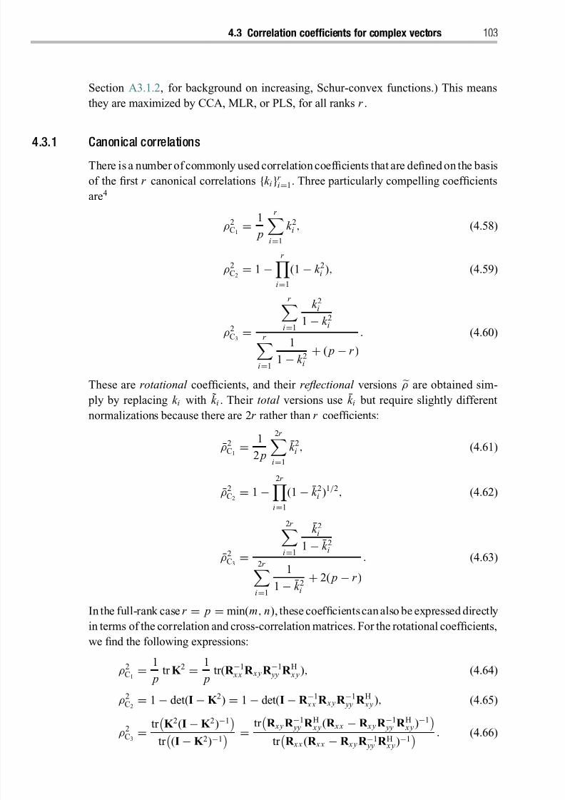
8/21/2019 Statistical Signal Processing of Complex-Valued Data.pdf
http://slidepdf.com/reader/full/statistical-signal-processing-of-complex-valued-datapdf 125/330
4.3 Correlation coefficients for complex vectors 103
Section A3.1.2, for background on increasing, Schur-convex functions.) This means
they are maximized by CCA, MLR, or PLS, for all ranks r .
4.3.1 Canonical correlations
There is a number of commonly used correlation coefficients that are defined on the basis
of the first r canonical correlations {k i}r i=1. Three particularly compelling coefficients
are4
ρ2C1= 1
p
r i=1
k 2i , (4.58)
ρ2C2
=1
−
r
i=1
(1
−k 2i ), (4.59)
ρ2C3=
r i=1
k 2i
1 − k 2ir
i=1
1
1 − k 2i+ ( p − r )
. (4.60)
These are rotational coefficients, and their reflectional versions
ρ are obtained sim-
ply by replacing k i with k i . Their total versions use k i but require slightly different
normalizations because there are 2r rather than r coefficients:
ρ2C1= 1
2 p
2r i=1
k 2i , (4.61)
ρ2C2= 1 −
2r i=1
(1 − k 2i )1/2, (4.62)
ρ2
C3 =
2r
i=1
k 2i
1
− k 2i
2r i=1
1
1 − k 2i+ 2( p − r )
. (4.63)
In the full-rank case r = p = min(m, n), these coefficientscan also be expressed directly
in terms of the correlation and cross-correlation matrices. For the rotational coefficients,
we find the following expressions:
ρ2C1= 1
ptr K 2 = 1
ptr(R −1
x x R x y R −1 yy R H x y), (4.64)
ρ2C2 = 1 − det(I − K
2
) = 1 − det(I − R −1
x x R x y R −1
yy R H x y), (4.65)
ρ2C3= tr
K 2(I − K 2)−1
tr (I − K 2)−1
= tr
R x y R −1 yy R H x y(R x x − R x y R −1
yy R H x y)−1
tr
R x x (R x x − R x y R −1 yy R H x y)−1
. (4.66)
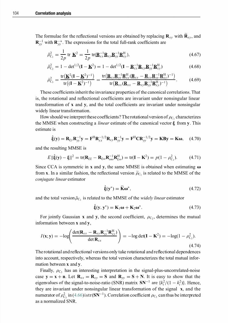
8/21/2019 Statistical Signal Processing of Complex-Valued Data.pdf
http://slidepdf.com/reader/full/statistical-signal-processing-of-complex-valued-datapdf 126/330
104 Correlation analysis
The formulae for the reflectional versions are obtained by replacing R x y with R x y , and
R −1 yy with R −∗ yy . The expressions for the total full-rank coefficients are
ρ
2
C1 =1
2 p tr K
2
=1
2 p tr(R −1
x x R x y R −1
yy R
H
x y), (4.67)
ρ2C2= 1 − det1/2(I − K 2) = 1 − det1/2(I − R −1
x x R x y R −1 yy R H x y) (4.68)
ρ2C3= tr
K 2(I − K 2)−1
tr (I − K 2)−1
= tr
R x y R −1 yy R H x y(R x x − R x y R −1
yy R H x y)−1
tr
R x x (R x x − R x y R −1 yy R H x y)−1
. (4.69)
These coefficients inherit the invariance properties of the canonical correlations. That
is, the rotational and reflectional coefficients are invariant under nonsingular linear
transformation of x and y, and the total coefficients are invariant under nonsingular
widely linear transformation.How should we interpret thesecoefficients? The rotationalversion of ρC1 characterizes
the MMSE when constructing a linear estimate of the canonical vector from y. This
estimate is
(y) = R ξ y R −1 yy y = FHR −1/2
x x R x y R −1 yy y = FHCR −1/2
yy y = KBy = K , (4.70)
and the resulting MMSE is
E (y) − 2 = tr(R ξ ξ − R ξ ωR −1ωωR Hξ ω) = tr(I − K 2) = p(1 − ρ2
C1). (4.71)
Since CCA is symmetric in x and y, the same MMSE is obtained when estimating
from x. In a similar fashion, the reflectional version ρC1 is related to the MMSE of the
conjugate linear estimator
(y∗) = K ∗, (4.72)
and the total version ρC1 is related to the MMSE of the widely linear estimator
(y, y∗) = K 1 + K 2∗. (4.73)
For jointly Gaussian x and y, the second coefficient, ρC2, determines the mutual
information between x and y,
I (x; y) = −log
det(R x x − R x y R −1
yy R H x y)
det R x x
= −log det(I − K 2) = −log(1 − ρ2
C2).
(4.74)
The rotational and reflectional versionsonly take rotational and reflectional dependences
into account, respectively, whereas the total version characterizes the total mutual infor-
mation between x and y.
Finally, ρC3 has an interesting interpretation in the signal-plus-uncorrelated-noise
case y = x + n. Let R x x = R x y = S and R yy = S + N. It is easy to show that the
eigenvalues of the signal-to-noise-ratio (SNR) matrix SN−1 are {k 2i /(1 − k 2i )}. Hence,they are invariant under nonsingular linear transformation of the signal x, and the
numerator of ρ2C3
in (4.66)istr(SN−1). Correlation coefficient ρC3 can thus be interpreted
as a normalized SNR.
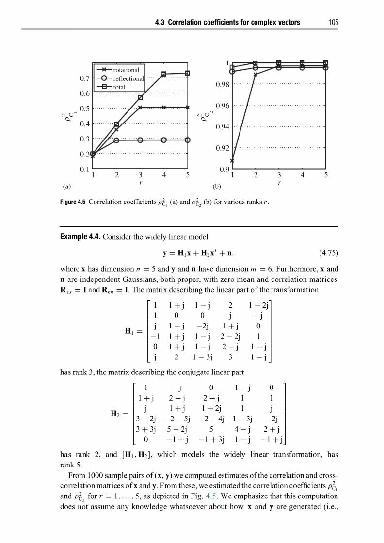
8/21/2019 Statistical Signal Processing of Complex-Valued Data.pdf
http://slidepdf.com/reader/full/statistical-signal-processing-of-complex-valued-datapdf 127/330
4.3 Correlation coefficients for complex vectors 105
1
(a) (b)
2 3 4 50.1
0.2
0.3
0.4
0.5
0.6
0.7
r
r C
1 2
rotational
reflectional
total
1 2 3 4 50.9
0.92
0.94
0.96
0.98
1
r
r C
2 2
Figure 4.5 Correlation coefficients ρ 2C1
(a) and ρ 2C2
(b) for various ranks r .
Example 4.4. Consider the widely linear model
y = H1x + H2x∗ + n, (4.75)
where x has dimension n = 5 and y and n have dimension m = 6. Furthermore, x and
n are independent Gaussians, both proper, with zero mean and correlation matrices
R x x = I and R nn = I. The matrix describing the linear part of the transformation
H1 =
1 1 + j 1 − j 2 1 − 2j
1 0 0 j − j
j 1 − j −2j 1 + j 0
−1 1 + j 1 − j 2 − 2j 1
0 1 + j 1 − j 2 − j 1 − j
j 2 1 − 3j 3 1 − j
has rank 3, the matrix describing the conjugate linear part
H2 =
1 − j 0 1 − j 0
1 + j 2 − j 2 − j 1 1
j 1 + j 1 + 2j 1 j
3 − 2j −2 − 5j −2 − 4j 1 − 3j −2j
3 + 3j 5 − 2j 5 4 − j 2 + j
0 −1 + j −1 + 3j 1 − j −1 + j
has rank 2, and [H1, H2], which models the widely linear transformation, has
rank 5.
From 1000 sample pairs of (x, y) we computed estimates of the correlation and cross-correlation matrices of x and y. From these, we estimated the correlation coefficients ρ2
C1
and ρ2C2
for r = 1, . . . , 5, as depicted in Fig. 4.5. We emphasize that this computation
does not assume any knowledge whatsoever about how x and y are generated (i.e.,
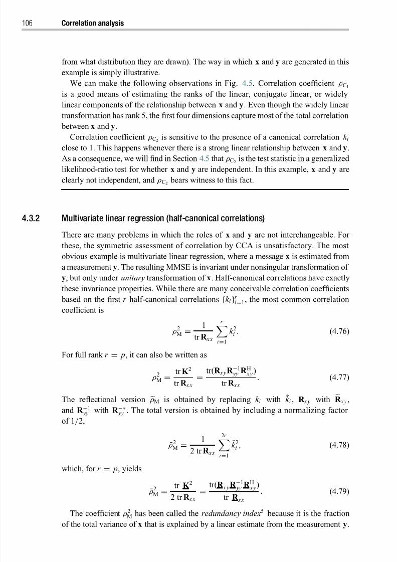
8/21/2019 Statistical Signal Processing of Complex-Valued Data.pdf
http://slidepdf.com/reader/full/statistical-signal-processing-of-complex-valued-datapdf 128/330
106 Correlation analysis
from what distribution they are drawn). The way in which x and y are generated in this
example is simply illustrative.
We can make the following observations in Fig. 4.5. Correlation coefficient ρC1
is a good means of estimating the ranks of the linear, conjugate linear, or widely
linear components of the relationship between x and y. Even though the widely linear
transformation has rank 5, the first four dimensions capture most of the total correlation
between x and y.
Correlation coefficient ρC2 is sensitive to the presence of a canonical correlation k i
close to 1. This happens whenever there is a strong linear relationship between x and y.
As a consequence, we will find in Section 4.5 that ρC2 is the test statistic in a generalized
likelihood-ratio test for whether x and y are independent. In this example, x and y are
clearly not independent, and ρC2 bears witness to this fact.
4.3.2 Multivariate linear regression (half-canonical correlations)
There are many problems in which the roles of x and y are not interchangeable. For
these, the symmetric assessment of correlation by CCA is unsatisfactory. The most
obvious example is multivariate linear regression, where a message x is estimated from
a measurement y. The resulting MMSE is invariant under nonsingular transformation of
y, but only under unitary transformation of x. Half-canonical correlations have exactly
these invariance properties. While there are many conceivable correlation coefficients
based on the first r half-canonical correlations {k i }r i=1, the most common correlation
coefficient is
ρ2M =
1
tr R x x
r i=1
k 2i . (4.76)
For full rank r = p, it can also be written as
ρ2M =
tr K 2
tr R x x
= tr(R x y R −1 yy R H x y)
tr R x x
. (4.77)
The reflectional version ρM is obtained by replacing k i with k i , R x y with R x y ,
and R −1 yy with R −∗ yy . The total version is obtained by including a normalizing factor
of 1/2,
ρ2M =
1
2 tr R x x
2r i=1
k 2i , (4.78)
which, for r = p, yields
ρ2M =
tr K 2
2 tr R x x=
tr(R x y R −1 yy R H x y)
tr R x x. (4.79)
The coefficient ρ2M has been called the redundancy index5 because it is the fraction
of the total variance of x that is explained by a linear estimate from the measurement y.
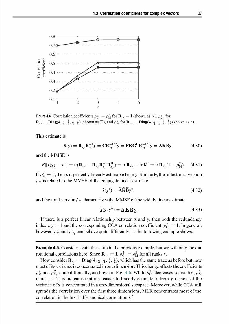
8/21/2019 Statistical Signal Processing of Complex-Valued Data.pdf
http://slidepdf.com/reader/full/statistical-signal-processing-of-complex-valued-datapdf 129/330
4.3 Correlation coefficients for complex vectors 107
1 2 3 4 50.1
0.2
0.3
0.4
0.5
C o r r e l a t i o n
c o e f f i c i e n t 0.6
0.7
0.8
r
Figure 4.6 Correlation coefficients ρ 2C1= ρ2
M for R x x = I (shown as ×), ρ 2C1
for
R x x = Diag(4, 14
, 14
, 14
, 14) (shown as ), and ρ2
M for R x x = Diag(4, 14
, 14
, 14
, 14) (shown as ◦).
This estimate is
x(y) = R x y R −1 yy y = CR −1/2
yy y = FKGHR −1/2 yy y = AKBy, (4.80)
and the MMSE is
E
x(y)
−x
2
=tr(R x x
−R x y R −1
yy R H x y)
=tr R x x
−tr K 2
=tr R x x (1
−ρ2
M). (4.81)
If ρ2M = 1, then x is perfectly linearly estimable from y. Similarly, the reflectional versionρM is related to the MMSE of the conjugate linear estimate
x(y∗) = AK By∗, (4.82)
and the total version ρM characterizes the MMSE of the widely linear estimate
x(y, y∗) = A K B y. (4.83)
If there is a perfect linear relationship between x and y, then both the redundancy
index ρ
2
M = 1 and the corresponding CCA correlation coefficient ρ
2
C1 = 1. In general,however, ρ 2
M and ρ 2C1
can behave quite differently, as the following example shows.
Example 4.5. Consider again the setup in the previous example, but we will only look at
rotational correlations here. Since R x x = I, ρ 2C1= ρ2
M for all ranks r .
Now consider R x x = Diag(4, 14
, 14
, 14
, 14), which has the same trace as before but now
most of its variance is concentrated in onedimension. This change affects thecoefficients
ρ2M and ρ 2
C1quite differently, as shown in Fig. 4.6. While ρ 2
C1decreases for each r , ρ 2
M
increases. This indicates that it is easier to linearly estimate x from y if most of the
variance of x is concentrated in a one-dimensional subspace. Moreover, while CCA stillspreads the correlation over the first three dimensions, MLR concentrates most of the
correlation in the first half-canonical correlation k 21 .
8/21/2019 Statistical Signal Processing of Complex-Valued Data.pdf
http://slidepdf.com/reader/full/statistical-signal-processing-of-complex-valued-datapdf 130/330
108 Correlation analysis
4.3.3 Partial least squares
For problemsthat are invariantunder unitarytransformation of x and y, the mostcommon
correlation coefficient is defined in terms of the PLS correlations
{k i
}r i
=1 as
ρ2P =
r i=1
k 2i
√ tr R 2 x x tr R 2 yy
. (4.84)
This coefficient was proposed by Robert and Escoufier (1976). For r = p, it can be
expressed as
ρ2P =
tr K 2√ tr R 2 x x tr R 2 yy
= tr(R x y R H x y)√ tr R 2 x x tr R 2 yy
. (4.85)
This correlation coefficient measures how closely x and y are related under unitarytransformation. For y = Ux, with UHU = I but not necessarily UUH = I, we haveperfect
correlation ρ 2P = 1.
The reflectional version ρP is obtained by replacing k i with k i and R x y with R x y .
The total version, which is invariant under widely unitary transformation of x and
y, is
ρ2P
=
2r i=1
k 2i
√ tr R 2 x x tr R 2 yy
. (4.86)
In the full-rank case r = p, this yields
ρ2P =
tr K 2√ tr R 2 x x tr R 2 yy
= tr(R x y R H x y)√ tr R 2 x x tr R 2 yy
. (4.87)
4.4 Correlation spread
Using the results from Appendix 3, Section A3.2, it is not difficult to show thatall correlation coefficients presented in this chapter are Schur-convex and increas-
ing functions of the diagonal cross-correlations {k i }. By maximizing all partial
sums over their absolute values, subject to the constraints imposed by the correla-
tion analysis technique, the correlation coefficients are then also maximized for all
ranks r .
Theimportance of this result is that we may assesscorrelation in a low(er)-dimensional
subspace of dimension r < p. In fact, the development in this chapter anticipates some
closely related results on reduced-rank estimation, which we will study in Section
5.5. There we will find that canonical coordinates are the optimum coordinate systemfor reduced-rank estimation and transform coding if the aim is to maximize informa-
tion rate, whereas half-canonical coordinates are the optimum coordinate system for
8/21/2019 Statistical Signal Processing of Complex-Valued Data.pdf
http://slidepdf.com/reader/full/statistical-signal-processing-of-complex-valued-datapdf 131/330
4.4 Correlation spread 109
reduced-rank estimation and transform coding if we want to minimize mean-squared
error.
An interesting question in this context is how much of the overall correlation is cap-
tured by r coefficients{
k i}
r
i=1, which can be rotational, reflectional, or total coefficients
defined either through CCA, MLR, or PLS. One could, of course, compute the frac-
tion ρ 2(r )/ρ2( p) for all 1 ≤ r < p. The following definition, however, provides a more
convenient approach.
Definition 4.4. The rotational correlation spread is defined as
σ 2 = 1
p
var({k 2i })µ2({k 2i })
= p
p − 1
p
i=1
k 4i pi=1
k 2i
2 − 1
p
, (4.88)
where var({k 2i }) denotes the variance of the correlations {k 2i } and µ2({k 2i }) denotes their
squared mean.
The correlation spread provides a single, normalized measure of how concentrated
the overall correlation is. If there is only one nonzero coefficient k 1, then σ 2
= 1. If all coefficients are equal, k 1 = k 2 = · · · = k p, then σ 2 = 0. In essence, the correlation
spread gives an indication of how compressible the cross-correlation between x and y is.
The definition (4.88) is inspired by the definition of the degree of polarization of a
random vector x. The degree of polarization measures the spread among the eigenvalues
of R x x . A random vector x is said to be completely polarized if all of its energy is
concentrated in one direction, i.e., if there is only one nonzero eigenvalue. On the other
hand, x is unpolarized if its energy is equally distributed among all dimensions, i.e., if all
eigenvalues are equal. The correlation spread σ 2 generalizes this idea to the correlation
between two random vectors x and y.
Example 4.6. Continuing Example 4.5 for R x x = I, we find σ 2C = σ 2M = 0.167 for both
CCA and MLR. For R x x = Diag(4, 14
, 14
, 14
, 14), we find σ 2C = 0.178 for CCA and σ 2M =
0.797forMLR.A σ 2-value close to1 indicates that the correlation ishighly concentrated.
Indeed, as we have found in Example 4.5, most of the MLR correlation is concentrated
in a one-dimensional subspace.
The reflectional correlation spread is defined as a straightforward extension by replac-ing k 2i with k 2i in Definition 4.4, but the total correlation spread is defined in a slightly
different manner.
8/21/2019 Statistical Signal Processing of Complex-Valued Data.pdf
http://slidepdf.com/reader/full/statistical-signal-processing-of-complex-valued-datapdf 132/330
110 Correlation analysis
Definition 4.5. The total correlation spread is defined as
σ 2
=
1
p
var
12(k 22i−1 + k 22i )
µ2 1
2 (¯k
2
2i−1 + ¯k
2
2i ) (4.89)
= p
p − 1
p
i=1
(k 22i−1 + k 22i )2
pi=1
k 22i−1 + k 22i
2 − 1
p
. (4.90)
The motivation for defining σ 2 in this way is twofold. First, since k 2i−1 is the cross-
correlation between the real parts and k 2i is the cross-correlation between the imaginary
parts of ξ i and ωi , they belong to the same complex dimension. Secondly, the expression
(4.90) becomes (4.88) if k 2i−1 = k 2i = k i for all i .
4.5 Testing for correlation structure
In practice, correlation matrices will be estimated from measurements. Given these
estimates, how can we make informed decisions such as whether x is white, or whether x
and y areindependent? Questionssuch as thesemust beanswered byemployingstatisticaltests for correlation structure. In this section, we develop generalized likelihood-ratio
tests (GLRTs) for complex Gaussian data.6 That is, we assume that the data can be
modeled as a complex Gaussian random vector x: −→ Cn with probability density
function
p(x) = 1
π n det R x x
exp−(x − x )HR −1
x x (x − x )
, (4.91)
mean x , and covariance matrix R x x . Later we will also replace x with other vectors
such as [xT
, yT
]T
. We note that (4.91) is a proper Gaussian pdf, and the story we will betelling here is strictly linear, for simplicity. Appropriate extensions exist for augmented
vectors, where the pdf (4.91) is adapted by replacing det with det1/2 and including a
factor of 1/2 in the quadratic form of the exponential (cf. Result 2.4). These two changes
to the pdf have no significant consequences for the following development.
Consider M independent and identically distributed (i.i.d.) random samples X =[x1, x2, . . . , x M ] drawn from this distribution. The joint probability density function of
these samples is given by
p(X) = π− Mn (det R x x )− M exp− M m=1
(xm − x )HR −1 x x (xm − x ) (4.92)
= π− Mn (det R x x )− M exp− M tr(R −1
x x S x x )
, (4.93)
8/21/2019 Statistical Signal Processing of Complex-Valued Data.pdf
http://slidepdf.com/reader/full/statistical-signal-processing-of-complex-valued-datapdf 133/330
4.5 Testing for correlation structure 111
where S x x is the sample covariance matrix
S x x =1
M
M
m=1
(xm − m x )(xm − m x )H = 1
M XXH − m x mH
x (4.94)
and m x is the sample mean vector
m x =1
M
M m=1
xm . (4.95)
We would now like to test whether R x x has structure 0 or the alternative structure 1. We
write this hypothesis-testing problem as
H 0: R x x ∈ R0,
H 1: R x x ∈ R1.
The GLRT statistic is
λ =max
R xx ∈R0
p(X)
maxR xx ∈R1
p(X). (4.96)
This ratio compares the likelihood of drawing the samples x1, . . . , x M from a distribution
whose covariance matrix has structure 0 with the likelihood of drawing them from
a distribution whose covariance matrix has structure 1. Since the actual covariance
matrices arenotknown, theyarereplaced with theirmaximum-likelihood(ML) estimates
computed from the samples. If we denote by R 0 the ML estimate of R x x under H 0 and
by R 1 the ML estimate of R x x under H 1, we find
λ = det M R −1
0 R 1
exp− M tr
R −10 S x x − R −1
1 S x x
. (4.97)
If we further assume that R1 is the set of positive semidefinite matrices (i.e., no special
constraints are imposed), then R 1 = S x x , and
λ
=det M
R −10 S x xexp Mn
− M tr R −1
0 S x x. (4.98)
This may be expressed in the following result, which is Theorem 5.3.2 in Mardia et al .
(1979).
Result 4.9. The generalized likelihood ratio for testing whether R x x has structure
R0 is
= λ1/( Mn ) = g e1−a (4.99)
where a and g are the arithmetic and geometric means of the eigenvalues of
R −1
0 S x x :
a = 1n
tr R −10 S x x, (4.100)
g =det R −1
0 S x x
1/n
. (4.101)
8/21/2019 Statistical Signal Processing of Complex-Valued Data.pdf
http://slidepdf.com/reader/full/statistical-signal-processing-of-complex-valued-datapdf 134/330
112 Correlation analysis
In the hypothesis-testing problem, a threshold 0 is chosen to achieve a desired prob-
ability of false alarm or probability of detection. Then, if ≥ 0, we accept hypothesis
H 0, and if < 0, we reject it.
The GLRT is always invariant with respect to transformations for which the
hypothesis-testing problem itself is invariant. The GLR will therefore turn out to
be a function of a maximal invariant , which is determined by the hypothesis-testing
problem. Let’s consider a few interesting special cases.
4.5.1 Sphericity
We would like to test whether x has a spherical distribution, i.e.,
R0 = {R x x = σ 2
x I}, (4.102)
where σ 2 x is the variance of each component of x. The ML estimate of R x x under H 0 is R 0 = σ 2 x I, where the variance is estimated as σ 2 x = n−1 tr S x x . The GLR in Result 4.9 is
therefore
= [det S x x ]1/n
1ntr S x x
. (4.103)
This test is invariantwith respect to scale and unitary transformation. That is, x
−→αUx
with α ∈ C and unitary U ∈ Cn×n leaves the GLR unchanged. The GLR is therefore a
function of a maximal invariant under scale and unitary transformation. Such a maximal
invariant is the set of estimated eigenvalues of R x x (i.e., the eigenvalues of S x x ), denoted
by {λi}ni=1, normalized by tr S x x :
λi
tr S x x
n
i=1
.
Indeed, we can express the GLR as
(n)n =n
i=1
λi
tr S x x
, (4.104)
which also allows a reduced-rank implementation of the GLRT by considering only the
r largest estimated eigenvalues.
4.5.2 Independence within one data set
Now we would like to test whether x has independent components, i.e., whether R x x is
diagonal:
R0 = {R x x = Diag( R11, R22, . . . , Rnn )}. (4.105)
8/21/2019 Statistical Signal Processing of Complex-Valued Data.pdf
http://slidepdf.com/reader/full/statistical-signal-processing-of-complex-valued-datapdf 135/330
4.5 Testing for correlation structure 113
The ML estimate of R x x under H 0 is R 0 = Diag (S 11, S 22, . . . , S nn ), where S ii is the i th
diagonal element of S x x . The GLR in Result 4.9 is therefore the Hadamard ratio
n
=det S x x
ni=1
S ii
. (4.106)
This test is invariant with respect to multiplication with a nonsingular diagonal matrix.
That is, x −→ Dx with nonsingular diagonal D ∈ Cn×n leaves the GLR unchanged.
The GLR is therefore a function of a maximal invariant under multiplication with a
diagonal matrix. Such a maximal invariant is obtained as follows. Let Zii denote the
submatrix obtained from rows i + 1 through n and columns i + 1 through n of the
sample covariance matrix S x x . Let zi be the column-vector obtained from rows i + 1
through n in column i of the sample covariance matrix S x x . For i =
1, . . . , n−
1, they
can be combined in
Zi−1,i−1 =
S ii zHi
zi Zii
(4.107)
and Z00 = S x x . Now define
β2i =
zHi Z−1
i i zi
S i i
, i = 1, . . . , n − 1, (4.108)
β2n = 0. (4.109)
We notice that β2i is the estimated squared canonical correlation between the i th com- ponent of x and components i + 1 through n of x, and thus 0 ≤ β2
i ≤ 1. It can be shown
that the set {β2i }n−1
i=1 is the maximal invariant we are looking for. Indeed, we can express
the GLR as
n =
ni=1
S ii (1 − β2i )
n
i=1
S ii
=n−1i=1
(1 − β2i ), (4.110)
which also allows a reduced-rank implementation of the GLRT by considering only the
r largest estimated canonical correlations β2i .
4.5.3 Independence between two data sets
Now replace x with the composite vector [xT, yT]T, where x: −→ Cn and y: −→Cm , and replace R x x with the composite covariance matrix of x and y:
R x y =
R x x R x y
R H x y R yy. (4.111)
We would like to test whether x and y are independent , i.e., whether x and y have a
block-diagonal composite covariance matrix R x y with R x y = 0:
R0 =R x y =
R x x 0
0 R yy
. (4.112)
8/21/2019 Statistical Signal Processing of Complex-Valued Data.pdf
http://slidepdf.com/reader/full/statistical-signal-processing-of-complex-valued-datapdf 136/330
114 Correlation analysis
The ML estimate of R x y under H 0 is
R0 =
S x x 0
0 S yy. (4.113)
The GLR in Result 4.9 is therefore
n = det
I S−1
x x S x y
S−1 yy SH
x y I
= det(I − S−1
x x S x y S−1 yy SH
x y). (4.114)
This test is invariant with respect to multiplication of x and y, each with a nonsingular
matrix. That is, x −→ Nx and y −→ My for nonsingular N ∈ Cn×n and M ∈ Cm×m
leaves the GLR unchanged. A maximal invariant for these invariances is, of course, the
set of canonical correlations. Hence, the GLR can also be written as
n = pi=1
(1 − k 2i ) = 1 − ρ2C2
, (4.115)
where p = min(m, n), {k i } pi=1 are the estimated canonical correlations between x and y,
computed from the sample covariances, and ρ2C2
is the estimated correlation coefficient
defined in (4.59). This expression allows a reduced-rank implementation of theGLRT by
considering only the r largest estimated canonical correlations. The test for impropriety
in Section 3.4 is a special case of the test presented here, where y = x∗. However, the test
for impropriety tests for uncorrelatedness between x and x∗ rather than independence: x
and x∗ cannot be independent because x∗ is perfectly determined by x through complexconjugation.7
Notes
1 Since the assessment of multivariate association between random vectors is of importance in
many research areas, there is a rich literature on this topic. Canonical correlation analysis is the
oldest technique, which was invented by Hotelling (1936). Partial least squares was introduced
by Wold (1975) in the field of chemometrics but our description of it follows a different variant
suggested by Sampson et al . (1989).
Much of this chapter, in particular the discussion of majorization and correlation spread,
closely follows Schreier (2008c). This paper is cIEEE, and portions are used with permission.
An excellent unifying discussion of correlation analysis techniques with emphasis on their
invariance properties is given by Ramsay et al . (1984). Different research areas often use quite
different jargon, and we have attempted to use terms that are as generic as possible.
2 To the best of our knowledge, there are not many papers on correlation analysis of complex
data. Usually, the analysis of rotational and reflectional correlations proceeds in terms of real
data of double dimension rather than complex data, see, for instance, Jupp and Mardia (1980).
Hanson et al . (1992) proposed working directly with complex data when analyzing rotational
and reflectional dependences.
3 Many definitions of correlation coefficients (see, e.g., Renyi (1959)) require the symmetry
ρ x y = ρ yx . However, this does notseem like a fundamental requirement. In fact, if thecorrelation
analysis technique itself is not symmetric (as for instance is the case for MLR) it would not be
reasonable to ask for symmetry in correlation coefficients based on it.

8/21/2019 Statistical Signal Processing of Complex-Valued Data.pdf
http://slidepdf.com/reader/full/statistical-signal-processing-of-complex-valued-datapdf 137/330
Notes 115
4 Correlation coefficients based on CCA were discussed by Rozeboom (1965), Coxhead (1974),
Yanai (1974), and Cramer and Nicewander (1979).
5 The redundancy index, which is based on MLR, was analyzed by Stewart and Love (1968) and
Gleason (1976).
6 Section 4.5 draws on material from Mardia et al . (1979). A general introduction to likelihood-ratio tests is provided in Section 7.1.
7 Much more can be done in Section 4.5. There are the obvious extensions to augmented vectors
and widely linear transformations. The results of Sections 4.5.2 and 4.5.3 can be combined
to test for block-diagonal structure with more than two diagonal blocks. Then hypothesis tests
that have the invariance properties of half-canonical correlations and partial least squares can
be developed, for which half-canonical correlations and partial least-squares correlations will
be the maximal invariants. Finally, we have completely ignored the distributional properties of
the GLRT statistics. The moments of the statistic in (4.114) are well known, cf. Mardia et al .
(1979) and Lehmann and Romano (2005). The latter reference provides more background on
the rich topic of hypothesis testing.
8/21/2019 Statistical Signal Processing of Complex-Valued Data.pdf
http://slidepdf.com/reader/full/statistical-signal-processing-of-complex-valued-datapdf 138/330
5 Estimation
One of the most important applications of probability in science and engineering is
to the theory of statistical inference, wherein the problem is to draw defensible con-
clusions from experimental evidence. The three main branches of statistical inference
are parameter estimation, hypothesis testing , and time-series analysis. Or, as we say in
the engineering sciences, the three main branches of statistical signal processing are
estimation, detection, and signal analysis.
A common problem is to estimate the value of a parameter, or vector of parameters,
from a sequence of measurements. The underlying probability law that governs the
generation of the measurements depends on the parameter. Engineering language would
say that a source of information, loosely speaking, generates a signal x and a channel
carries this information in a measurement y, whose probability law p(y|x) depends on
the signal. There is usually little controversy over this aspect of the problem because
the measurement scheme generally determines the probability law. There is, however, a
philosophical divide about the modeling of the signal x. Frequentists adopt the point of
view that to assign a probability law to the signal assumes too much. They argue that the
signal should be treated as an unknown constant and the data should be allowed to speak
for itself. Bayesians argue that the signal should be treated as a random variable whose
prior probability distribution is to be updated to a posterior distribution as measurements
are made.
In the realm of exploratory data analysis and in the absence of a physical model for
the experiment or measurement scheme, the difference between these points of view is
profound. But, for most problems of parameter estimation and hypothesis testing in theengineering and applied sciences, the question resolves itself on the basis of physical
reasoning, either theoretical or empirical. For example, in radar, sonar, and geophysical
imaging, the question of estimating a signal, or resolving a hypothesis about the signal,
usually proceeds without the assignment of a probability law or the assignment of a prior
probability to the hypothesis that a nonzero signal will be returned. The point of view is
decidedly frequentist. On the other hand, in data communication, where the problem is
to determine which signal from a set of signals was transmitted, it is quite appropriate
to assign prior probabilities to elements of the set. The appropriate view is Bayesian.
Finally, in most problemsof engineering andapplied science, measurements areplentiful by statistical standards, and the weight of experimental evidence overwhelms the prior
model, making the practical distinction between the frequentist and the Bayesian a
philosophical one of marginal practical effect.
8/21/2019 Statistical Signal Processing of Complex-Valued Data.pdf
http://slidepdf.com/reader/full/statistical-signal-processing-of-complex-valued-datapdf 139/330
5.1 Hilbert-space geometry 117
In this chapter on estimation, we shall be interested, by and large, in linear and widely
linear least-squares problems, wherein parameter estimators are constrained to be linear
or widely linear in the measurement and the performance criterion is mean-squared
error or squared error under a constraint. The estimators we compute are then linear
or widely linear minimum mean-squared error (LMMSE or WLMMSE) estimators.
These estimators strike a balance between frequentism and Bayesianism by using only
second-order statistical models for signal and noise. When the underlying joint dis-
tribution between the measurement y and the signal x is multivariate Gaussian, these
estimators are also conditional mean and maximum a-posteriori likelihood estimators
that would appeal to a Bayesian. No matter what your point of view is, the result-
ing estimators exploit all of the Hermitian and complementary correlation that can be
exploited, within the measurements, within the signals, and between the signals and
measurements.
As a prelude to our development of estimators, Section 5.1 establishes a Hilbert-space
geometry for augmented random variables that will be central to our reasoning about
WLMMSE estimators. We then review a few fundamental results for MMSE estimation
in Section 5.2, without the constraint that the estimator be linear or widely linear. From
there we proceed to the development of linear channel and filtering models, since these
form the foundation for LMMSE estimation, which is discussed in Section 5.3. Most of
these results translate to widely linear estimation in a straightforward fashion, but it is
still worthwhile to point out a few peculiarities of WLMMSE estimation and compare it
with LMMSE estimation, which is done in Section 5.4. Section 5.5 considers reduced-
rank widely linear estimators, which either minimize mean-squared error or maximize
information rate. We derive linear and widely linear minimum-variance distortionless
response (MVDR) receivers in Section 5.6. These estimators assign no statistical model
to the signal, and therefore appeal to the frequentist. Finally, Section 5.7 presents widely
linear-quadratic estimators.
5.1 Hilbert-space geometry of second-order random variables
The Hilbert space geometry of random variables is based on second-order moment properties only. Why should such a geometry be important in applications? The obvious
answer is that the dimension of signals to be estimated is generally small and the
dimension of measurements large, so that quality estimates can be obtained from sample
means and generalizations of these that are based on correlation structure. The subtle
answer is that the geometry of second-order random variables enables us to exploit a
comfortable imagery and intuition based on our familiarity with Euclidean geometry.
An algebraic approach to Euclidean geometry, often called analytic geometry, is
founded on the concept of an inner product between two vectors. To exploit this point of
view, we will have to think of a random variable as a vector. Then norm, distance, and orthogonality can be defined in terms of inner products.
A random experiment is modeled by the sample space , where each point ω ∈
corresponds to a possible outcome, and a probability measure P on . The probability
8/21/2019 Statistical Signal Processing of Complex-Valued Data.pdf
http://slidepdf.com/reader/full/statistical-signal-processing-of-complex-valued-datapdf 140/330
118 Estimation
measure associates with each event A (a measurable subset of ) a probability
P ( A). A random variable x is a measurable function x : −→ C, which assigns
each outcome ω ∈ a complex number x . The set of second-order random vari-
ables (for which E | x|2 <
∞) forms a Hilbert space with respect to the inner product
defined as
x, y = E ( x∗ y) =
x∗(ω) y(ω)d P (ω), (5.1)
which is the correlation between x and y . We may thus identify the space of second-order
random variables with the space of square-integrable functions L2(, P ). This space is
closed under addition and multiplication by complex scalars. From this inner product,
we obtain the following geometrical quantities:
the norm (length) of a random variable x : x =
√ x , x
= E | x|2,
the distance between two random variables x and y: x − y = √ x − y, x − y = E | x − y|2,
the angle between two random variables x and y:
cos2α = | x , y |2 x2 y2
= | E ( x∗ y)|2 E | x|2 E | y|2 ,
orthogonality: x and y are orthogonal if x, y = E ( x∗ y) = 0, the Cauchy–Schwarz inequality: | x, y| ≤ x y, i.e., | E ( x∗ y)| ≤
E | x|2 E | y|2.
The random variable x may be replaced by the random variable x ∗, in which case theinner product is the complementary correlation
x∗, y = E ( x y) =
x(ω) y(ω)d P (ω). (5.2)
This inner product is nonzero if and only if x and y are cross-improper. For y = x
the complementary correlation is x∗, x = E x2, which is nonzero if and only if x is
improper. It follows from the Cauchy–Schwarz inequality that | E x2| ≤ E | x|2.
In the preceding chapters we have worked with augmented random variables x =[ x, x∗]T, which are measurable functions x:
−→C2
∗. The vector space C2
∗ contains
all complex pairs of the form [ x , x∗]T. It is a real linear (or complex widely linear )
subspace of C2 because it is closed under addition and multiplication with a real scalar,
but not with a complex scalar. The inner product for augmented random variables isx, y
= E (xHy) = 2 Re E ( x∗ y) = 2 Re x, y, (5.3)
which amounts to taking (twice) the real part of the inner product between x and y. In
this book, we use all three inner products, x, y, x∗, y, and
x, y.
Example 5.1. Let x be a real random variable and y a purely imaginary random variable.Theinner product x , y is generally nonzero, but it must be purely imaginary. Therefore,
x, y = 2 Re x, y = 0. This means that x and y are orthogonal even though x and y
might not be.

8/21/2019 Statistical Signal Processing of Complex-Valued Data.pdf
http://slidepdf.com/reader/full/statistical-signal-processing-of-complex-valued-datapdf 141/330
5.2 Minimum mean-squared error estimation 119
If z = x + y, we may perfectly reconstruct x from z . This, however, requires the
widely linear operation x = Re z , which assumes that we know the phase of z . It is not
generally possible to perfectly reconstruct x from z using strictly linear operations.
The preceding generalizes to random vectors x = [ x1, x2, . . . , xn]T: −→ Cn and
x = [xT, xH]T: −→ C2n∗ . Let H (x) denote the Hilbert space of second-order aug-
mented random vectors x. The Euclidean view characterizes the angle between span-
ning vectors in terms of a Grammian matrix, consisting of all inner products between
vectors. In the Hilbert space H (x), this Grammian matrix consists of all inner products
of the form E ( x∗i x j ) and E ( xi x j ). We have come to know this Grammian matrix as the
augmented correlation matrix of x:
R x x = E (x x
H
) = E x
x∗ xH
xT = R x x R x xR ∗ x x R ∗ x x. (5.4)
It is commonplace in adaptive systems to use a vector of N realizations si ∈ C N of
a random variable x i to estimate the Hilbert-space inner products E ( x∗i x j ) and E ( xi x j )
by the Euclidean inner products N −1sHi s j and N −1sT
i s j .
There is one more connection to be made with Euclidean spaces. Given two sets of
(deterministic) spanning vectors S = [s1, s2, . . . , sn] and R = [r1, r2, . . . , rn], we may
define the cosines of the principal angles between their linear subspaces S and R as
the singular values of the matrix (SHS)−1/2SHR (R HR )−H/2. In a similar way we define
the cosines of the principal angles between the subspaces H (x) and H (y) as the singular values of the matrix R −1/2 x x R x y R −H/2
yy , whicharecalled thecanonical correlations between
x and y. They were introduced in Section 4.1. We will use them again in Section 5.5 to
develop reduced-rank linear estimators.
5.2 Minimum mean-squared error estimation
The general problem we address here is the estimation of a complex random vector x
from a complex random vector y. As usual we think of x as the signal or source, and y
as the measurement or observation. Presumably, y carries information about x that can
be extracted with an estimation algorithm.
We begin with the consideration of an arbitrary estimator x, which is a function
of y, and its mean-squared error matrix Q = E [(x − x)(x − x)H]. We first expand the
expression for Q using the conditional mean E [x|y] – which is itself a random vector
since it depends on y – as
Q = E [(x − E [x|y] + E [x|y] − x)(x − E [x|y] + E [x|y] − x)H], (5.5)
where the outer E stands for expectation over the joint distribution of x and y. We may
then write
Q = E [( E [x|y] − x)( E [x|y] − x)H] + E [(x − E [x|y])( E [x|y] − x)H]
+ E [( E [x|y] − x)(x − E [x|y])H] + E [(x − E [x|y])(x − E [x|y])H]. (5.6)
8/21/2019 Statistical Signal Processing of Complex-Valued Data.pdf
http://slidepdf.com/reader/full/statistical-signal-processing-of-complex-valued-datapdf 142/330
120 Estimation
The third term is of the form E [( E [x|y] − x)gH(y)] with g(y) = x − E [x|y]. Using the
law of total expectation, we see that this term vanishes:
E
{ E [( E [x
|y]
−x)gH(y)
|y]
} =0. (5.7)
The same reasoning can be applied to conclude that the second term in (5.6) is also zero.
Therefore, the optimum estimator, obtained by making the fourth term in (5.6) equal to
zero, turns out to be the conditional mean estimator x = E [x|y]. Let
e = x − x = E [x|y] − x (5.8)
be the error vector. Its mean E [e] = 0, and thus E [x] = E [x]. This says that x is an
unbiased estimator of x. The covariance matrix of the error vector is
Q = E [eeH] = E [( E [x|y] − x)( E [x|y] − x)H]. (5.9)
Any competing estimator x with mean-squared error matrix Q = E [eeH] = E [(x −x)(x − x)H] will be suboptimum in the sense that Q ≥ Q, meaning that Q − Q is
positive semidefinite. As a consequence, the conditional mean estimator is a minimum
mean-squared error (MMSE) estimator:
E e2 = tr Q ≤ tr Q = E e2. (5.10)
But we can say more. For the class of real-valued increasing functions of matrices,
Q ≤ Q implies f (Q) ≤ f (Q). Thus we have the following result.
Result 5.1. The conditional mean estimator E [x|y] minimizes (maximizes) any increas-ing (decreasing) function of the mean-squared error matrix Q.
Besides the trace, the determinant is another example of an increasing function. Thus,
the volume of the error covariance ellipsoid is also minimized:
det Q ≤ det Q. (5.11)
A very important property of the MMSE estimator is the so-called orthogonality
principle, a special case of which we have already encountered in the derivation (5.7).
However, it holds much more generally.
Result 5.2. The error vector e is orthogonal to every measurable function of y , g(y).
That is, E [egH(y)] = E {( E [x|y] − x)gH(y)} = 0.
For g(y) = E [x|y], this orthogonality condition says that the estimator error e is
orthogonal to the estimator E [x|y]. Moreover, since the conditional mean estimator
is an idempotent operator Px = E [x|y] – which is to say that P2x = E { E [x|y]|y} = E [x|y] = Px – we may think of the conditional mean estimator as a projection operator
that orthogonally resolves x into its estimator E [x|y] minus its estimator error e:
x=
E [x|y]−
( E [x|y]−
x). (5.12)
The conditional mean estimator summarizes everything of use for MMSE estimation
of x from y. This means conditioning x on y and y∗ would change nothing, since this has
already been done, so to speak, in the conditional mean E [x|y]. Similarly the conditional
8/21/2019 Statistical Signal Processing of Complex-Valued Data.pdf
http://slidepdf.com/reader/full/statistical-signal-processing-of-complex-valued-datapdf 143/330
5.3 Linear MMSE estimation 121
mean estimator of x∗ is just the complex conjugate of the conditional mean estimator
of x. Thus it makes no sense to consider the estimation of x from y and y∗, since this
brings no refinement to the conditional mean estimator. As we shall see, this statement
is decidedly false when the estimator is constrained to be a (widely) linear or (widely)
linear-quadratic estimator.
5.3 Linear MMSE estimation
We shall treat the problem of linearly or widely linearly estimating a signal from a mea-
surement as a virtual two-channel estimation problem, wherein the underlying exper-
iment consists of generating a composite vector of signal and measurement, only one
of which is observed.1 Our point of view is that the augmented covariance matrix for
this composite vector then encapsulates all of the second-order information that can be
extracted. In order to introduce our methods, we shall begin here with the Hermitian
case, wherein complementary covariances are ignored, and then extend our methods to
include Hermitian and complementary covariances in the next section.
Let usbegin witha signal (or source) x: −→ Cn anda measurement vector y: −→Cm . There isno requirement that the signal dimension n besmaller than the measurement
dimension m. We first assume that the signal and measurement have zero mean, but
remove this restriction later on. Their composite covariance matrix is the matrix
R x y = E xy xH yH = R x x R x y
R H x y R yy. (5.13)
The error between the signal x and the linear estimator x = Wy is e = x − x and the
error covariance matrix is Q = E [(x − x)(x − x)H]. This error covariance is
Q = E [(Wy − x)(Wy − x)H] = WR yy WH − R x y WH − WR H x y + R x x . (5.14)
After completing the square, this may be written
Q = R x x − R x y R −1 yy R H x y + (W − R x y R −1
yy )R yy (W − R x y R −1 yy )H. (5.15)
This quadratic form in W is positive semidefinite, so Q ≥ R x x − R x y R −1 yy R H x y withequality for
W = R x y R −1 yy and Q = R x x − R x y R −1
yy R H x y . (5.16)
The solution for W may be written as the solution to the normal equations WR yy −R x y = 0, or more insightfully as2
E [(Wy − x)yH] = 0. (5.17)
Thus theorthogonality principle is at work: theestimatorerror e = Wy − x is orthogonal
to the measurement y, as illustrated in Fig. 5.1. There H (y) denotes the Hilbert space of measurement vectors y and orthogonality means E [(Wy − x)i y
∗ j ] = 0 for all pairs (i, j ).
Moreover, the linear operator W is a projection operator, since the LMMSE estimator
of x from Wy remains Wy. The LMMSE estimator is sometimes referred to as the

8/21/2019 Statistical Signal Processing of Complex-Valued Data.pdf
http://slidepdf.com/reader/full/statistical-signal-processing-of-complex-valued-datapdf 144/330
122 Estimation
H (y)Wy
ex
Figure 5.1 Orthogonality between the error e = Wy − x and H (y) in LMMSE estimation.
(c)(b)y
H
H
y
x x
H
(a)n
x xyx
nn
Figure 5.2 The signal-plus-noise channel model: (a) channel, (b) synthesis, and (c) analysis.
(discrete) Wiener filter , which explains our choice of notation W. However, the LMMSE
estimator predates Wiener’s work on causal LMMSE prediction and smoothing of time
series.
5.3.1 The signal-plus-noise channel model
We intend to argue that it is as if the source and measurement vectors were drawn from a
linear channel model y = Hx + n that draws a source vector x, linearly filters the source
vector with a channel filter H, and adds an uncorrelated noise vector n to produce the
measurement vector. This scheme is illustrated with the signal-plus-noise channel model
of Fig. 5.2(a). According to this channel model, the source and measurement have the
synthesis and analysis representations of Figs. 5.2( b) and (c):x
y
=
I 0
H I
x
n
, (5.18)
x
n
=
I 0
−H I
x
y
. (5.19)
The synthesis model of Fig. 5.2( b) and the analysis model of Fig. 5.2(c) produce these
block LDU (Lower triangular–Diagonal–Upper triangular) Cholesky factorizations:
R x y = R x x R x y
R H x y R yy
= I 0H I
R x x 00 R nn
I HH
0 I, (5.20)
R x x 0
0 R nn
=
I 0
−H I
R x x R x y
R H x y R yy
I −HH
0 I
. (5.21)
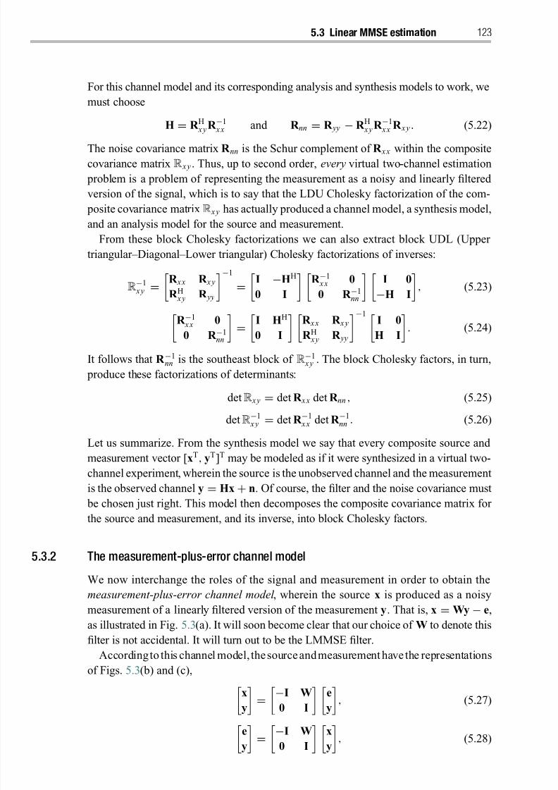
8/21/2019 Statistical Signal Processing of Complex-Valued Data.pdf
http://slidepdf.com/reader/full/statistical-signal-processing-of-complex-valued-datapdf 145/330
5.3 Linear MMSE estimation 123
For this channel model and its corresponding analysis and synthesis models to work, we
must choose
H
=R H x y R −1
x x and R nn
=R yy
−R H x y R −1
x x R x y . (5.22)
The noise covariance matrix R nn is the Schur complement of R x x within the composite
covariance matrix R x y . Thus, up to second order, every virtual two-channel estimation
problem is a problem of representing the measurement as a noisy and linearly filtered
version of the signal, which is to say that the LDU Cholesky factorization of the com-
posite covariance matrixR x y has actually produced a channel model, a synthesis model,
and an analysis model for the source and measurement.
From these block Cholesky factorizations we can also extract block UDL (Upper
triangular–Diagonal–Lower triangular) Cholesky factorizations of inverses:
R−1 x y = R x x R x y
R H x y R yy
−1 = I −HH
0 I R −1 x x 0
0 R −1nn
I 0
−H I, (5.23)
R −1
x x 0
0 R −1nn
=
I HH
0 I
R x x R x y
R H x y R yy
−1 I 0
H I
. (5.24)
It follows that R −1nn is the southeast block of R−1
x y . The block Cholesky factors, in turn,
produce these factorizations of determinants:
detR x y = det R x x det R nn , (5.25)
detR−1 x y = det R −1
x x det R −1nn . (5.26)
Let us summarize. From the synthesis model we say that every composite source and
measurement vector [xT, yT]T may be modeled as if it were synthesized in a virtual two-
channel experiment, wherein the source is the unobserved channel and the measurement
is the observed channel y = Hx + n. Of course, the filter and the noise covariance must
be chosen just right. This model then decomposes the composite covariance matrix for
the source and measurement, and its inverse, into block Cholesky factors.
5.3.2 The measurement-plus-error channel model
We now interchange the roles of the signal and measurement in order to obtain the
measurement-plus-error channel model , wherein the source x is produced as a noisy
measurement of a linearly filtered version of the measurement y. That is, x = Wy − e,
as illustrated in Fig. 5.3(a). It will soon become clear that our choice of W to denote this
filter is not accidental. It will turn out to be the LMMSE filter.
Accordingto this channel model, thesourceandmeasurement have the representations
of Figs. 5.3( b) and (c),
xy = −I W
0 I e
y, (5.27)
e
y
=−I W
0 I
x
y
, (5.28)
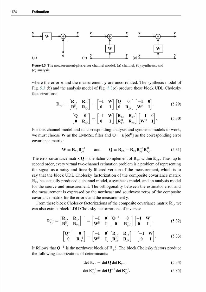
8/21/2019 Statistical Signal Processing of Complex-Valued Data.pdf
http://slidepdf.com/reader/full/statistical-signal-processing-of-complex-valued-datapdf 146/330
124 Estimation
(b) (c)(a) y
e
y
e
e
y x
W
y
x
W
W
y
x
Figure 5.3 The measurement-plus-error channel model: (a) channel, (b) synthesis, and
(c) analysis
where the error e and the measurement y are uncorrelated. The synthesis model of
Fig. 5.3 (b) and the analysis model of Fig. 5.3(c) produce these block UDL Cholesky
factorizations:
R x y = R x x R x y
R H x y R yy = −I W
0 I Q 0
0 R yy −I 0
WH I, (5.29)
Q 0
0 R yy
=−I W
0 I
R x x R x y
R H x y R yy
−I 0
WH I
. (5.30)
For this channel model and its corresponding analysis and synthesis models to work,
we must choose W as the LMMSE filter and Q = E [eeH] as the corresponding error
covariance matrix:
W
=R x y R −1
yy and Q
=R x x
−R x y R −1
yy R H x y . (5.31)
The error covariance matrix Q is the Schur complement of R yy within R x y . Thus, up to
second order, every virtual two-channel estimation problem is a problem of representing
the signal as a noisy and linearly filtered version of the measurement, which is to
say that the block UDL Cholesky factorization of the composite covariance matrix
R x y has actually produced a channel model, a synthesis model, and an analysis model
for the source and measurement. The orthogonality between the estimator error and
the measurement is expressed by the northeast and southwest zeros of the composite
covariance matrix for the error e and the measurement y.
From these block Cholesky factorizations of the composite covariance matrixR x y wecan also extract block LDU Cholesky factorizations of inverses:
R−1 x y =
R x x R x y
R H x y R yy
−1
=−I 0
WH I
Q−1 0
0 R −1 yy
−I W
0 I
, (5.32)
Q−1 0
0 R −1 yy
=−I 0
WH I
R x x R x y
R H x y R yy
−1 −I W
0 I
. (5.33)
It follows that Q−1 is the northwest block of R−1 x y . The block Cholesky factors produce
the following factorizations of determinants:
detR x y = det Q det R yy , (5.34)
detR−1 x y = det Q−1 det R −1
yy . (5.35)

8/21/2019 Statistical Signal Processing of Complex-Valued Data.pdf
http://slidepdf.com/reader/full/statistical-signal-processing-of-complex-valued-datapdf 147/330
5.3 Linear MMSE estimation 125
Let us summarize. From the analysis model we say that every composite signal and
measurement vector [xT, yT]T may be modeled as if it were a virtual two-channel
experiment, wherein the signal is subtracted from a linearly filtered measurement to
produce an error that is orthogonal to the measurement. Of course, the filter and the
error covariance must be chosen just right. This model then decomposes the composite
covariance matrix for the signal and measurement, and its inverse, into block Cholesky
factors.
5.3.3 Filtering models
We might say that the models we have developed give us two alternative parameteriza-
tions:
the signal-plus-noise channel model (R x x , H, R nn ) with H = R H x y R −1 x x and R nn =R yy − R H x y R −1
x x R x y ; and the measurement-plus-error channel model (R yy , W, Q) with W = R x y R −1
yy and Q =R x x − R x y R −1
yy R H x y .
These correspond to the two factorizations (A1.2) and (A1.1) of R x y , and R nn and Q
are the Schur complements of R x x and R yy , respectively, within R x y . Let’s mix the
synthesis equation for the signal-plus-noise channel model with the analysis equation of
the measurement-plus-error channel model to solve for the filter W and error covariance
matrix Q in terms of the channel parameters H and R nn :e
y
=−I W
0 I
I 0
H I
x
n
. (5.36)
This composition of maps produces these factorizations:Q 0
0 R yy
=−I W
0 I
I 0
H I
R x x 0
0 R nn
I HH
0 I
−I 0
WH I
, (5.37)
Q−1 0
0 R −1 yy
=−I 0
WH I I −HH
0 I R −1
x x 0
0 R −1nn
I 0
−H I
−I W
0 I . (5.38)
We now evaluate the northeast block of (5.37) and the southwest block of (5.38) to obtain
two formulae for the filter W:
W = R x x HH(HR x x HH + R nn )−1 = (R −1 x x + HHR −1
nn H)−1HHR −1nn . (5.39)
In a similar fashion, we evaluate the northwest blocks of both (5.37) and (5.38) to get
two formulae for the error covariance Q:
Q = R x x − R x x HH(HR x x HH + R nn )−1HR x x = (R −1 x x + HHR −1
nn H)−1. (5.40)
These equations are Woodbury identities, (A1.43) and (A1.44). They determine theLMMSE inversion of the measurement y for the signal x. In the absence of noise, if the
signal and measurement were of the same dimension, then W would be H−1, assuming
that this inverse existed. However, generally WH = I, but is approximately so if R nn is
8/21/2019 Statistical Signal Processing of Complex-Valued Data.pdf
http://slidepdf.com/reader/full/statistical-signal-processing-of-complex-valued-datapdf 148/330
126 Estimation
small compared with HR x x HH. The LMMSE estimator may be written as
Wy = W(Hx + n) = WHx + Wn. (5.41)
So, the LMMSE estimator W, sometimes called a deconvolutionfilter, decidedly doesnotequalize H to produce WH = I. Rather, it approximatesI so that the error e = Wy − x =(WH − I)x + Wn, with covariance matrix Q = (WH − I)R x x (WH − I)H + WR nn WH
provides the best tradeoff between model-bias-squared (WH − I)R x x (WH − I)H and
filtered noise variance WR nn WH to minimize the error covariance Q. The importance
of these results cannot be overstated.
Let us summarize. Every problem of LMMSE estimation requiring only first- and
second-order moments can be phrased as a problem of estimating one unobserved
channel from another observed channel in a virtual two-channel experiment. In this
virtual two-channel experiment, there are two different channel models.The first channel model says it is as if the measurement were a linear combination
of filtered source and uncorrelated additive noise. The second channel model says it is
as if the source vector were a linear combination of the filtered measurement and the
estimator error.
The first channel model produces a block LDU Cholesky factorization for the com-
posite covariance matrix R x y and a block UDL Cholesky factorization for its inverse.
The second channel model produces a block UDL Cholesky factorization for the com-
posite covariance matrix R x y and a block LDU Cholesky factorization for its inverse.
By mixing these two factorizations, two different solutions are found for the LMMSEestimator and its error covariance.
Example 5.2. In many problems of signal estimation in communication, radar, and sonar,
or imaging in geophysics and radio astronomy, the measurement model may be taken to
be the rank-one linear model
y = x + n, (5.42)
where ∈ Cm is the channel vector that carries the unknown complex signal amplitude
x to the measurement, x is a zero-mean random variable with variance σ 2 x , and R nn is the
covariance matrix of the noise vector n. Using the results of the previous subsections,
we may write down the following formulae for the LMMSE estimator of x and its
mean-squared error:
ˆ x = σ 2 x H(σ 2 x H + R nn )−1y = (σ −2 x + HR −1
nn )−1HR −1nn y, (5.43)
Q = σ 2 x − σ 4 x H(σ 2 x H + R nn )−1 = 1
σ −2 x
+HR −1
nn . (5.44)
In both forms the estimator consists of a matrix inverse operator, followed by a
correlator, followed by a scalar multiplication. When the channel filter is a vector’s worth
of a geometric sequence, = [1, e jθ , . . . , e jmθ ]T, as in a uniformly sampled complex
8/21/2019 Statistical Signal Processing of Complex-Valued Data.pdf
http://slidepdf.com/reader/full/statistical-signal-processing-of-complex-valued-datapdf 149/330
5.3 Linear MMSE estimation 127
exponential time series or a uniformly sampled complex exponential plane wave, then
the correlation step is a correlation with a discrete-time Fourier-transform (DTFT)
vector.
5.3.4 Nonzero means
We have assumed until now that the signal and measurement have zero means. What if
the signal has known mean x and the measurement has known mean y? How do these
filtering formulae change? The centered signal and measurement x − x and y − y
then share the composite covariance matrix R x y . So the LMMSE estimator of x − x
from y − y should obey all of the equations already derived. That is,
x − x = W(y − y) ⇔ x = W(y − y) + x . (5.45)
But what about the orthogonality principle which says that the error between the
estimator and the signal is orthogonal to the measurement? This is still so due to
E [(x− x)yH]= E {[x− x − (x − x )](y − y)H}+ E {[x − x − (x − x )]H y } = 0.
(5.46)
The first term on the right is zero due to the orthogonality principle already established
for zero-mean LMMSE estimators. The second term is zero because x is an unbiased
estimator of x, i.e., E [x] = x .
5.3.5 Concentration ellipsoids
Let’s call B x x = {x: xHR −1 x x x = 1} the concentration ellipsoid for the signal vector x.
For scalar x , this is the circle B x x = { x : | x|2 = R x x}. The concentration ellipsoid for
the error vector e is Bee = {e: eHQ−1e = 1}. From the equation Q = R x x − R x y R −1 yy R H x y
we know that R x x ≥ Q and hence R −1 x x ≤ Q−1. The posterior concentration ellipsoid
Bee is therefore smaller than, and completely embedded within, the prior concentration
ellipsoid B x x . When the signal and measurement are jointly Gaussian, these ellipsoids
are probability-density contour lines (level curves).
Among measures of effectiveness for LMMSE are relative values for the trace and
determinant of Q and R x x . Various forms of these may be derived from the matrix
identities obtained from the channel models. They may be given insightful forms in
canonical coordinate systems, as we will see in Section 5.5. One particularly illuminating
formula is the gain of LMMSE filtering, which is closely related to mutual information
(cf. Section 5.5.2):
det R x x
det Q =det R yy
det R nn. (5.47)
So the gain of LMMSE estimation is the ratio of the volume of the measurement
concentration ellipsoid to the volume of the noise concentration ellipsoid.
8/21/2019 Statistical Signal Processing of Complex-Valued Data.pdf
http://slidepdf.com/reader/full/statistical-signal-processing-of-complex-valued-datapdf 150/330
128 Estimation
Example 5.3. Let’s consider the problem of linearly estimating the zero-mean signal
x from the zero-mean measurement y when the measurement is in fact the complex
conjugate of the signal, namely y
=x∗. The MMSE estimator is obviously the widely
linear estimator x = y∗ and its error covariance matrix is Q = 0.
The composite covariance matrix for x and x∗ is the augmented covariance matrix
R x x . From the structure of this matrix, namely
R x x =
R x x R x xR ∗ x x R ∗ x x
,
we know that the LMMSE estimator of x from x∗ is x = R x x R −∗ x x x∗, with error covariance
matrix Q = R x x −
R x x R −∗ x x
R ∗ x x . This error covariance matrix satisfies the inequality
0≤
Q≤
R x x . Of course, if x is proper, R x x
=0, then linear MMSE estimation is no
good at all. But, for improper signals, the error concentration ellipsoid for the error
e = x − x lies inside the concentration ellipsoid for x.
5.3.6 Special cases
Two special cases of LMMSE estimation warrant particular attention: the pure signal-
plus-noise case and the Gaussian case.
Signal plus noise
The pure signal-plus-noise problem is y = x + n, with H = I and x and n uncorrelated.
As a consequence, R x y = R x x , R yy = R x x + R nn , and the composite covariance matrix
is
R x y =
R x x R x x
R x x R x x + R nn
. (5.48)
The prior signal-plus-noise covariance is the series formula R yy = R x x + R nn , but the
posterior error covariance is the parallel formula Q = (R −1 x x + R −1
nn )−1. The gain of
LMMSE filtering is
det R x x
det Q= det(R x x + R nn )
det R nn
= det(I + R −1/2nn R x x R −H/2
nn ). (5.49)
The matrix R −1/2nn R x x R −H/2
nn can reasonably be called a signal-to-noise-ratio matrix.
These formulae are characteristic of LMMSE problems.
The Gaussian case
Suppose the signal and measurement are multivariate Gaussian, meaning that the com-
posite vector [xT, yT]T is multivariate normal with zero mean and composite covariance
matrix R x y . Then the conditional pdf for x, given y, is
p(x|y) = p(x, y)
p(y) = det R yy
π n detR x y
exp
xH yH
R−1
x y
x
y
− yHR −1
yy y
. (5.50)
8/21/2019 Statistical Signal Processing of Complex-Valued Data.pdf
http://slidepdf.com/reader/full/statistical-signal-processing-of-complex-valued-datapdf 151/330
5.4 Widely linear MMSE estimation 129
Using the identity detR x y = det R yy det Q and one of the Cholesky factors for R−1 x y , this
pdf may be written
p(x|y)=
1
π n det Qexp(x
−Wy)HQ−1(x
−Wy) . (5.51)
Thus the posterior pdf for x, given y, is Gaussian with conditional mean Wy and
conditional covariance Q. This means that the MMSE estimator – without the qualifier
that it be linear – is this conditional mean Wy, and its error covariance is Q.
5.4 Widely linear MMSE estimation
We have already established that widely linear transformations are required in order
to access the information contained in the complementary covariance matrix. In thissection,weconsiderwidely linear minimummean-squarederror (WLMMSE)estimation
of the zero-mean signal x: −→ Cn from the zero-mean measurement y: −→Cm . To extend our results for LMMSE estimation to WLMMSE estimation we need
only replace the signal x by the augmented signal x and the measurement y by the
augmented measurement y, specify the composite augmented covariance matrix for
these two vectors, and proceed as before. Nothing else changes. Thus, most of the results
from Section 5.3 apply straightforwardly to WLMMSE estimation. It is, however, still
worthwhile to summarizesome of these results and to compare LMMSE with WLMMSE
estimation.3
The widely linear (or linear–conjugate linear) estimator isx = W y ⇐⇒ x = W1y + W2y∗, (5.52)
where
W =
W1 W2
W∗2 W∗
1
(5.53)
is determined such that the mean-squared error
E x − x2 = 12 E x − x2 (5.54)
is minimized. This can be done by applying the orthogonality principle,
(x − x) ⊥ y and (x − x) ⊥ y∗, (5.55)
or (x − x) ⊥ y. This says that the error between the augmented estimator and the aug-
mented signal must be orthogonal to the augmented measurement. This leads to
E (x yH) − E (x yH) = 0,
W R yy − R x y = 0 ⇔ W = R x y R −1 yy . (5.56)
Using the matrix-inversion lemma (A1.42) for R −1 yy , we obtain the following result.
Result 5.3. Given an observation y: −→ Cm , the WLMMSE estimator of the signal
x: −→ Cn in augmented notation is
x = R x y R −1 yy y. (5.57)
8/21/2019 Statistical Signal Processing of Complex-Valued Data.pdf
http://slidepdf.com/reader/full/statistical-signal-processing-of-complex-valued-datapdf 152/330
130 Estimation
Equivalently,
x = (R x y −
R x y R −∗ yy
R ∗ yy )P−1
yy y + (
R x y − R x y R −1
yy
R yy )P−∗
yy y∗. (5.58)
In this equation, the Schur complement P yy = R yy − R yy R −∗ yy R ∗ yy is the error covariancematrix for linearly estimating y from y∗. The augmented error covariance matrix Q of
the error vector e = x − x is
Q = E [e eH] = R x x − R x y R −1 yy R H x y . (5.59)
A competing estimator x = Wy will produce an augmented error e = x − x with
covariance matrix
Q = E
eeH= Q + (W − W)R yy (W − W)H, (5.60)
which shows that Q≤
Q. As a consequence, all real-valued increasing functions of Q
are minimized, in particular,
E e2 = tr Q ≤ tr Q = E e2, (5.61)
det Q ≤ det Q. (5.62)
These statements hold for the error vector e as well as the augmented error vector e
because
Q ≤ Q ⇒ Q ≤ Q. (5.63)
The error covariance matrix Q of the error vector e = x − x is the northwest block of the augmented error covariance matrix Q, which can be evaluated as
Q = E [eeH] = R x x − (R x y − R x y R −∗ yyR ∗ yy )P−1
yy R H x y − (R x y − R x y R −1 yyR yy )P−∗
yyR H x y .
(5.64)
A particular choice for a generally suboptimum filter is the LMMSE filter
W =
R x y R −1 yy 0
0 R ∗ x y R −∗ yy
⇐⇒ W = R x y R −1
yy , (5.65)
which ignorescomplementarycovariance matrices.We willexaminetherelationbetween
LMMSE and WLMMSE filters in the following subsections.
5.4.1 Special cases
If the signal x is real , we have R x y = R ∗ x y . This leads to the simplified expression
x = 2 Re
(R x y − R x y R −∗ yyR ∗ yy )P−1
yy y
. (5.66)
While the WLMMSE estimate of a real signal is always real, the LMMSE estimate is
generally complex.
Result 5.4. The WLMMSE and LMMSE estimates are identical if and only if the error
of the LMMSE estimate is orthogonal to y∗ , i.e.,
(Wy − x) ⊥ y∗ ⇐⇒ R x y R −1 yyR yy − R x y = 0. (5.67)
8/21/2019 Statistical Signal Processing of Complex-Valued Data.pdf
http://slidepdf.com/reader/full/statistical-signal-processing-of-complex-valued-datapdf 153/330
5.4 Widely linear MMSE estimation 131
There are two important special cases in which (5.67) holds.
Thesignal andmeasurement arecross-proper,
R x y = 0, andthe measurement isproper,
R yy
=0. Joint propriety of x and y will suffice but it is not necessary that x be proper.
The measurement is maximally improper , i.e., y = αy∗ with probability 1 for con-stant α with |α| = 1. In this case, R x y = αR x y and R yy = αR yy and R x y R −1
yy R yy α −R x y α = 0. WL estimation is unnecessary since y and y∗ both carry exactly the same
information about x. This is irrespective of whether or not x is proper.
It may be surprising that (5.67) puts no restrictions on whether or not x be proper.
This is true for the performance criterion of MMSE. Other criteria such as weighted
MMSE or mutual information do depend on the complementary covariance matrix
of x.
Finally, the following result for Gaussian random vectors is now obvious bycomparing
x with x| y in (2.60) and Q with R x x| y in (2.61).
Result 5.5. Let x and y be two jointly Gaussian random vectors. The mean of the
conditional distribution for x given y is the WLMMSE estimator of x from y , and the
covariance matrix of the conditional distribution is the error covariance matrix of the
WLMMSE estimator.
5.4.2 Performance comparison between LMMSE and WLMMSE estimation
It is interesting to compare the performance of LMMSE and WLMMSE estimation. Wewill consider the signal-plus-uncorrelated-noise case y = x + n with white and proper
noise n, i.e., R nn = N 0I, R x y = R x x , and R yy = R x x + N 0I.
The LMMSE is
LMMSE = E e2 = tr(R x x − R x x (R x x + N 0I)−1R H x x )
=n
i=1
µi −
µ2i
µi + N 0
= N 0
ni=1
µi
µi + N 0, (5.68)
where {µi}ni=1 are the eigenvalues of R x x . On the other hand, the WLMMSE is
WLMMSE = E e2 = 12 tr (R x x − R x x (R x x + N 0I)−1R H x x )
= N 0
2
2ni=1
λi
λi + N 0, (5.69)
where {λi}2ni=1 are the eigenvalues of R x x . In order to evaluate the maximum perfor-
mance advantage of WLMMSE over LMMSE processing, we need to minimize theWLMMSE for fixed R x x and varying R x x . Using (A3.13) from Appendix 3, we see that
the WLMMSE is a Schur-concave function of the eigenvalues {λi }. Therefore, minimiz-
ing the WLMMSE requires maximum spread of the {λi } in the sense of majorization.
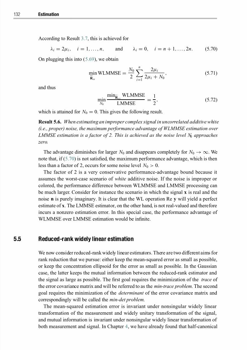
8/21/2019 Statistical Signal Processing of Complex-Valued Data.pdf
http://slidepdf.com/reader/full/statistical-signal-processing-of-complex-valued-datapdf 154/330
132 Estimation
According to Result 3.7, this is achieved for
λi = 2µi , i = 1, . . . , n, and λi = 0, i = n + 1, . . . , 2n. (5.70)
On plugging this into (5.69), we obtain
minR xx
WLMMSE = N 0
2
ni=1
2µi
2µi + N 0, (5.71)
and thus
min N 0
minR x xWLMMSE
LMMSE = 1
2, (5.72)
which is attained for N 0 = 0. This gives the following result.
Result 5.6. When estimating an improper complex signal in uncorrelated additive white(i.e., proper) noise, the maximum performance advantage of WLMMSE estimation over
LMMSE estimation is a factor of 2. This is achieved as the noise level N 0 approaches
zero.
The advantage diminishes for larger N 0 and disappears completely for N 0 → ∞. We
note that, if (5.70) is not satisfied, the maximum performance advantage, which is then
less than a factor of 2, occurs for some noise level N 0 > 0.
The factor of 2 is a very conservative performance-advantage bound because it
assumes the worst-case scenario of white additive noise. If the noise is improper or
colored, the performance difference between WLMMSE and LMMSE processing can
be much larger. Consider for instance the scenario in which the signal x is real and the
noise n is purely imaginary. It is clear that the WL operation Re y will yield a perfect
estimate of x. The LMMSE estimator, on the other hand, is not real-valued and therefore
incurs a nonzero estimation error. In this special case, the performance advantage of
WLMMSE over LMMSE estimation would be infinite.
5.5 Reduced-rank widely linear estimation
We now consider reduced-rank widely linear estimators. There are two different aims for
rank reduction that we pursue: either keep the mean-squared error as small as possible,
or keep the concentration ellipsoid for the error as small as possible. In the Gaussian
case, the latter keeps the mutual information between the reduced-rank estimator and
the signal as large as possible. The first goal requires the minimization of the trace of
the error covariance matrix and will be referred to as the min-trace problem. The second
goal requires the minimization of the determinant of the error covariance matrix and
correspondingly will be called the min-det problem.
The mean-squared estimation error is invariant under nonsingular widely linear transformation of the measurement and widely unitary transformation of the signal,
and mutual information is invariant under nonsingular widely linear transformation of
both measurement and signal. In Chapter 4, we have already found that half-canonical
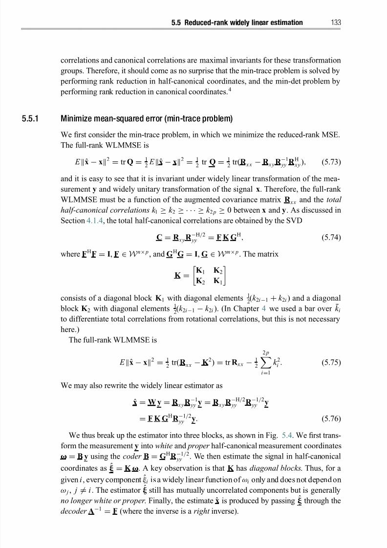
8/21/2019 Statistical Signal Processing of Complex-Valued Data.pdf
http://slidepdf.com/reader/full/statistical-signal-processing-of-complex-valued-datapdf 155/330
5.5 Reduced-rank widely linear estimation 133
correlations and canonical correlations are maximal invariants for these transformation
groups. Therefore, it should come as no surprise that the min-trace problem is solved by
performing rank reduction in half-canonical coordinates, and the min-det problem by
performing rank reduction in canonical coordinates.4
5.5.1 Minimize mean-squared error (min-trace problem)
We first consider the min-trace problem, in which we minimize the reduced-rank MSE.
The full-rank WLMMSE is
E x − x2 = tr Q = 12 E x − x2 = 1
2 tr Q = 1
2 tr(R x x − R x y R −1
yy R H x y), (5.73)
and it is easy to see that it is invariant under widely linear transformation of the mea-
surement y and widely unitary transformation of the signal x. Therefore, the full-rank WLMMSE must be a function of the augmented covariance matrix R x x and the total
half-canonical correlations k 1 ≥ k 2 ≥ · · · ≥ k 2 p ≥ 0 between x and y. As discussed in
Section 4.1.4, the total half-canonical correlations are obtained by the SVD
C = R x y R −H/2 yy = F K GH, (5.74)
where FHF = I, F ∈W n× p, and GHG = I, G ∈W m× p. The matrix
K =
K 1 K 2
K 2 K 1consists of a diagonal block K 1 with diagonal elements 1
2(k 2i−1 + k 2i ) and a diagonal
block K 2 with diagonal elements 12(k 2i−1 − k 2i ). (In Chapter 4 we used a bar over k i
to differentiate total correlations from rotational correlations, but this is not necessary
here.)
The full-rank WLMMSE is
E x − x2 = 12 tr(R x x − K 2) = tr R x x − 1
2
2 pi=1
k 2i . (5.75)
We may also rewrite the widely linear estimator as
x = W y = R x y R −1 yy y = R x y R −H/2
yy R −1/2 yy y
= F K GHR −1/2 yy y. (5.76)
We thus break up the estimator into three blocks, as shown in Fig. 5.4. We first trans-
form the measurement y into white and proper half-canonical measurement coordinates
= B y using the coder B = GHR −1/2 yy . We then estimate the signal in half-canonical
coordinates as = K . A key observation is that K has diagonal blocks. Thus, for a
given i , every component ξ i is a widely linear function of ωi only and does not depend onω j , j = i . The estimator still has mutually uncorrelated components but is generally
no longer white or proper . Finally, the estimate x is produced by passing through the
decoder A−1 = F (where the inverse is a right inverse).
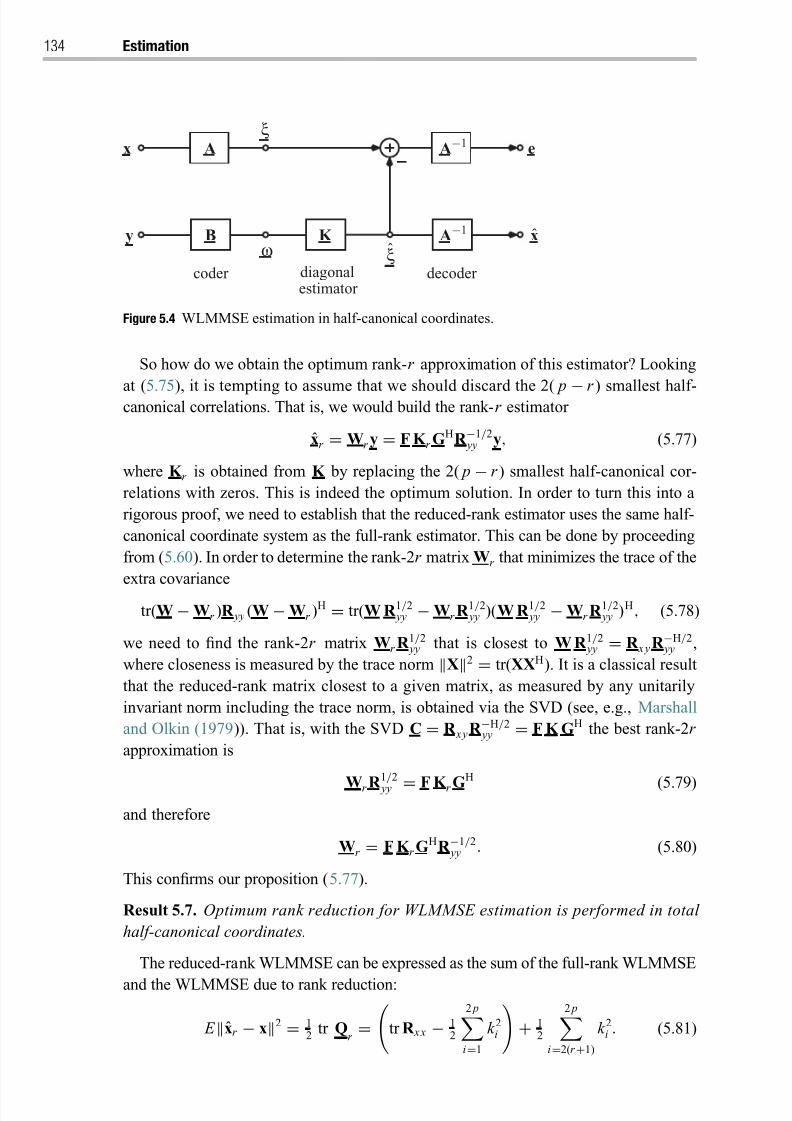
8/21/2019 Statistical Signal Processing of Complex-Valued Data.pdf
http://slidepdf.com/reader/full/statistical-signal-processing-of-complex-valued-datapdf 156/330
134 Estimation
decoder coder estimator diagonal
x
e
A−1
ξω K
A−1ξ
B
Ax
y
Figure 5.4 WLMMSE estimation in half-canonical coordinates.
So how do we obtain the optimum rank-r approximation of this estimator? Looking
at (5.75), it is tempting to assume that we should discard the 2( p − r ) smallest half-canonical correlations. That is, we would build the rank-r estimator
xr = Wr y = F K r GHR −1/2
yy y, (5.77)
where K r is obtained from K by replacing the 2( p − r ) smallest half-canonical cor-
relations with zeros. This is indeed the optimum solution. In order to turn this into a
rigorous proof, we need to establish that the reduced-rank estimator uses the same half-
canonical coordinate system as the full-rank estimator. This can be done by proceeding
from (5.60). In order to determine the rank-2r matrix Wr that minimizes the trace of the
extra covariance
tr(W − Wr )R yy (W − Wr )H = tr(W R 1/2
yy − Wr R 1/2 yy )(W R 1/2
yy − Wr R 1/2 yy )H, (5.78)
we need to find the rank-2r matrix Wr R 1/2 yy that is closest to W R 1/2
yy = R x y R −H/2 yy ,
where closeness is measured by the trace norm X2 = tr(XXH). It is a classical result
that the reduced-rank matrix closest to a given matrix, as measured by any unitarily
invariant norm including the trace norm, is obtained via the SVD (see, e.g., Marshall
and Olkin (1979)). That is, with the SVD C = R x y R −H/2 yy = F K GH the best rank-2r
approximation is
Wr R 1/2 yy = F K r G
H
(5.79)
and therefore
Wr = F K r GHR −1/2
yy . (5.80)
This confirms our proposition (5.77).
Result 5.7. Optimum rank reduction for WLMMSE estimation is performed in total
half-canonical coordinates.
The reduced-rank WLMMSE can be expressed as the sum of the full-rank WLMMSE
and the WLMMSE due to rank reduction:
E xr − x2 = 12 tr Q
r =
tr R x x − 12
2 pi=1
k 2i
+ 1
2
2 pi=2(r +1)
k 2i . (5.81)
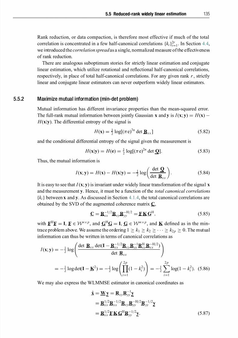
8/21/2019 Statistical Signal Processing of Complex-Valued Data.pdf
http://slidepdf.com/reader/full/statistical-signal-processing-of-complex-valued-datapdf 157/330
5.5 Reduced-rank widely linear estimation 135
Rank reduction, or data compaction, is therefore most effective if much of the total
correlation is concentrated in a few half-canonical correlations {k i }2r i=1. In Section 4.4,
we introduced the correlation spread as a single, normalized measure of the effectiveness
of rank reduction.
There are analogous suboptimum stories for strictly linear estimation and conjugate
linear estimation, which utilize rotational and reflectional half-canonical correlations,
respectively, in place of total half-canonical correlations. For any given rank r , strictly
linear and conjugate linear estimators can never outperform widely linear estimators.
5.5.2 Maximize mutual information (min-det problem)
Mutual information has different invariance properties than the mean-squared error.
The full-rank mutual information between jointly Gaussian x and y is I (x; y)=
H (x)− H (x|y). The differential entropy of the signal is
H (x) = 12 log[(π e)2n det R x x ] (5.82)
and the conditional differential entropy of the signal given the measurement is
H (x|y) = H (e) = 12 log[(π e)2n det Q]. (5.83)
Thus, the mutual information is
I (x; y)
= H (x)
− H (x
|y)
= −12 log
det Q
det R x x . (5.84)
It is easy to see that I (x; y) is invariant under widely linear transformation of the signal x
and the measurement y. Hence, it must be a function of the total canonical correlations
{k i } between x and y. As discussed in Section 4.1.4, the total canonical correlations are
obtained by the SVD of the augmented coherence matrix C,
C = R −1/2 x x R x y R −H/2
yy = F K GH, (5.85)
with FHF = I, F ∈W n× p, and GHG = I, G ∈W m× p, and K defined as in the min-
trace problem above. We assume the ordering 1 ≥ k 1 ≥ k 2 ≥ · · · ≥ k 2 p ≥ 0. The mutual
information can thus be written in terms of canonical correlations as
I (x; y) = − 12 log
det R x x det(I − R −1/2
x x R x y R −1 yy R H x y R −H/2
x x )
det R x x
= − 12 logdet(I − K 2) = − 1
2 log
2 p
i=1
(1 − k 2i )
= − 1
2
2 pi=1
log(1 − k 2i ). (5.86)
We may also express the WLMMSE estimator in canonical coordinates as
x=
W y=
R x y
R −1
yy
y
= R 1/2 x x R −1/2
x x R x y R −H/2 yy R −1/2
yy y
= R 1/2 x x F K GHR −1/2
yy y. (5.87)
8/21/2019 Statistical Signal Processing of Complex-Valued Data.pdf
http://slidepdf.com/reader/full/statistical-signal-processing-of-complex-valued-datapdf 158/330
136 Estimation
As in the previous section, this breaks up the estimator into three blocks. However,
this time we use a canonical coordinate system rather than a half-canonical coordi-
nate system. We first transform the measurement y into white and proper canonical
measurement coordinates =
B y using the coder B=
GHR −
1/2
yy . We then estimate
the signal in canonical coordinates as = K . While the estimator has mutually
uncorrelated components but is generally not white or proper , the canonical signal is
white and proper. Finally, the estimate x is produced by passing through the decoder
A−1 = F R 1/2 x x (where the inverse is a right inverse).
We now ask how to find a rank-r widely linear estimator that provides as much mutual
information about the signal as possible. Looking at (5.86), we are inclined to discard the
2( p − r ) smallest canonical correlations. We would thus construct the rank-r estimator
xr
=Wr y
=R 1/2
x x F K r GHR −1/2
yy y, (5.88)
which is similar to the solution of the min-trace problem (5.77) except that it uses a
canonical coordinate system in place of a half-canonical coordinate system. The rank-r
matrix K r is obtained from K by replacing the 2( p − r ) smallest canonical correlations
with zeros.
As in the min-trace case, our intuition is correct but it still requires a proof that
the reduced-rank maximum mutual information estimator does indeed use the same
canonical coordinate system as the full-rank estimator. The proof given below follows
Hua et al . (2001).
Starting from (5.60), maximizing mutual information means minimizing
det Qr = det(Q + (W − Wr )R yy (W − Wr )
H)
= det R x x det
I − C CH + (C − R −1/2 x x Wr R 1/2
yy )(C − R −1/2 x x Wr R 1/2
yy )H
.
(5.89)
For notational convenience, let
Xr = C − R −1/2 x x Wr R 1/2
yy . (5.90)
The minimum det Qr is zero if there is at least one canonical correlation k i equal to 1.
We may thus assume that all canonical correlations are strictly less than 1, which allowsus to write
det R x x det
I − C CH + Xr XHr
= det R x x det(I − C CH)det
I + (I − C CH)−1/2Xr X
Hr (I − C CH)−H/2
. (5.91)
Since det R x x and det(I − C CH) are independent of Wr , they can be disregarded in the
minimization. The third determinant in (5.91) is of the form
det(I+
Y YH)=
2 p
i=1
(1+
σ 2
i
), (5.92)
where {σ i }2 pi=1 are the singular values of Y = (I − C CH)−1/2Xr . This amounts to mini-
mizing Ywith respect to an arbitrary unitarily invariant norm. In other words, we need
to find the rank-2r matrix (I − C CH)−1/2R −1/2 x x Wr R 1/2
yy closest to (I − C CH)−1/2C. This
8/21/2019 Statistical Signal Processing of Complex-Valued Data.pdf
http://slidepdf.com/reader/full/statistical-signal-processing-of-complex-valued-datapdf 159/330
5.6 Linear and widely linear MVDR estimators 137
is achieved by a rank-2r SVD of (I − C CH)−1/2C. However, because the eigenvectors
of (I − C CH)−1/2 are the left singular vectors of C, a simpler solution is to use directly
the SVD of the augmented coherence matrix C = R −1/2 x x R x y R −H/2
yy = F K GH. The best
rank-2r approximation is thenR −1/2
x x Wr R 1/2 yy = F K r G
H (5.93)
and thus
Wr = R 1/2 x x F K r G
HR −1/2 yy . (5.94)
This confirms our initial claim.
Result 5.8. For Gaussian data, optimum rank reduction for widely linear maximum
information rate estimation is performed in total canonical coordinates.
The reduced-rank information rate is
I r (x; y) = − 12
2r i=1
log(1 − k 2i ), (5.95)
and the loss of information rate due to rank reduction is
I (x; y) − I r (x; y) = − 12
2 pi=2(r +1)
log(1 − k 2i ). (5.96)
Two remarks made in the min-trace case hold for the min-det case as well. Firstly,rank reduction is most effective if much of the total correlation is concentrated in a
few canonical correlations {k i}2r i=1. A good measure for the degree of concentration is
the correlation spread introduced in Section 4.4. Secondly, there are completely anal-
ogous, suboptimum, developments for strictly linear min-det estimation and conjugate
linear min-det estimation. These utilize rotational and reflectional canonical correla-
tions, respectively, in place of total canonical correlations. For any given rank, widely
linear min-det estimation is at least as good as strictly linear or conjugate linear min-det
estimation, but superior if the signals are improper.
5.6 Linear and widely linear minimum-variance distortionlessresponse estimators
In the engineering literature, especially in the fields of radar, sonar, and wireless com-
munication, it is commonplace to design a linear minimum-variance unbiased or linear
minimum variance-distortionless response(LMVDR)estimator(or receiver). Actually, it
would be more accurate to call these receivers best linear unbiased estimators (BLUEs),
which conforms to standard language in the statistics literature. In this section, we willfirst review the design and performance of the LMVDR receiver using Hermitian covari-
ances only, and then we shall extend our results to widely linear minimum-variance
distortionless response (WLMVDR) receivers by accounting for complementary
covariances.

8/21/2019 Statistical Signal Processing of Complex-Valued Data.pdf
http://slidepdf.com/reader/full/statistical-signal-processing-of-complex-valued-datapdf 160/330
138 Estimation
5.6.1 Rank-one LMVDR receiver
We shall begin by assuming the signal component of the received signal to lie in
a known one-dimensional subspace of C m , denoted
. We will later generalize to
p-dimensional subspaces Ψ. Without loss of generality we may assume H = 1,which is to say that is a unit vector. Thus the measurement model for the received
signal y: −→ Cm is
y = x + n, (5.97)
where the complex scalar x is unknown andtobe estimated, butmodeled as deterministic,
i.e., x is not assigned a probability distribution. The additive noise n is zero-mean with
Hermitian covariance matrix R nn = E [nnH]. The problem is to design a linear estimator
of x that is unbiased with variance smaller than any unbiased competitor. A first guess
would be the matched filter
ˆ x = Hy, (5.98)
which has mean E [ ˆ x] = x and variance
E [( ˆ x − x)( ˆ x − x)∗] = HR nn . (5.99)
This solution is linear and unbiased, but, as we now show, not minimum variance. To
design the LMVDR receiver ˆ x = wHy, let’s minimize its variance, under the constraint
that its mean be x :
min wHR nn w under constraint wH = 1. (5.100)
It is a simple matter to set up a Lagrangian, solve for the set of candidate solutions, and
enforce the constraint. This leads to the LMVDR receiver
ˆ x = HR −1nn
HR −1nn
y, (5.101)
which, for obvious reasons, is sometimes also called a whitened matched filter . This
solution too has mean E [ ˆ x] = x , but its variance is smaller:
Q = E [( ˆ x − x)( ˆ x − x)∗] = 1HR −1
nn . (5.102)
The inequality (HR −1nn )−1 ≤ HR nn is a special case of the Kantorovich inequality.
The LMVDR or BLUE estimator is also maximum likelihood when the measurement
noise n is zero-mean Gaussian with covariance R nn , in which case the measurement y
is Gaussian with mean x and covariance R nn .
Relation to LMMSE estimator
If the unknown variable x is modeled as in Example 5.2 as a random variable that is
uncorrelated with n and has zero mean and variance σ 2 x , then its LMMSE estimator is
ˆ x = HR −1nn
σ −2 x + HR −1
nn y. (5.103)
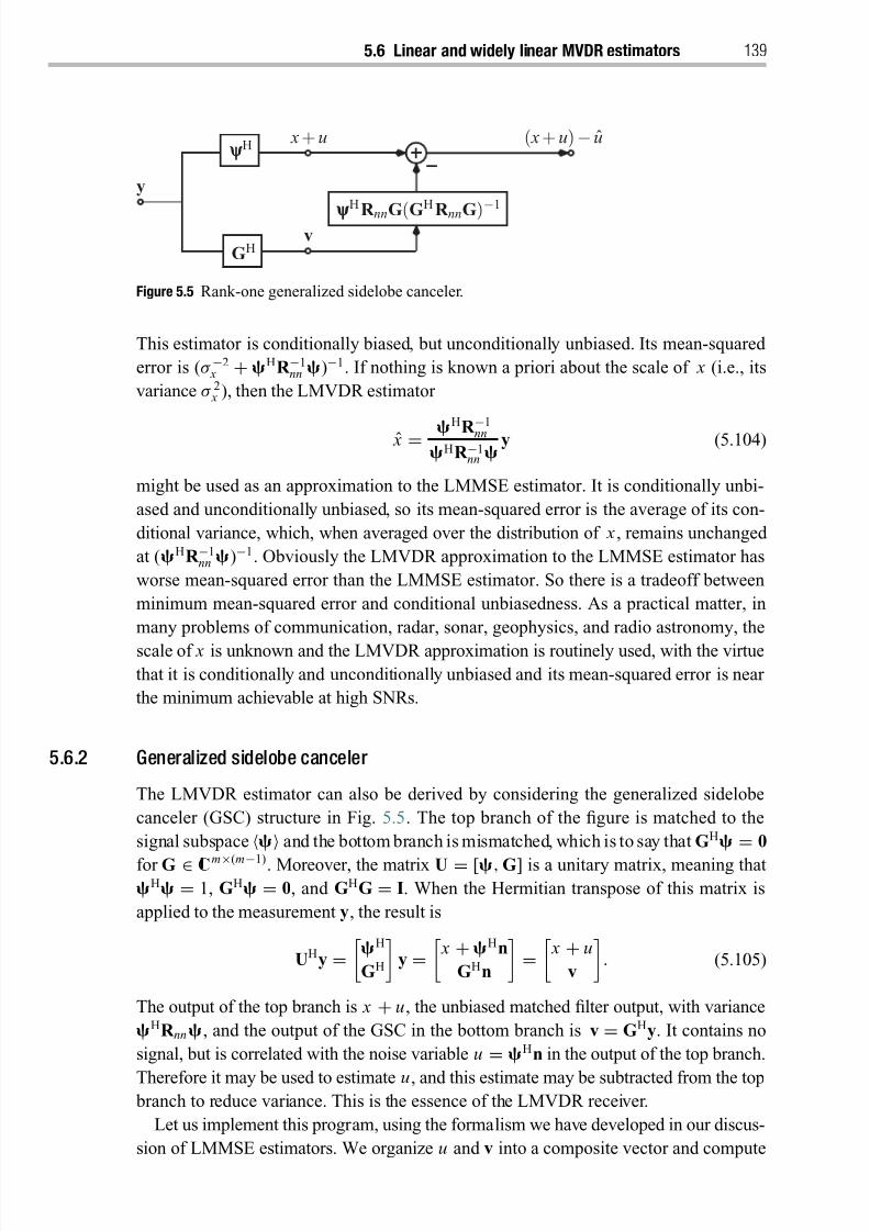
8/21/2019 Statistical Signal Processing of Complex-Valued Data.pdf
http://slidepdf.com/reader/full/statistical-signal-processing-of-complex-valued-datapdf 161/330
5.6 Linear and widely linear MVDR estimators 139
ψψ H
R nnG(GH
R nnG)−1
v
x+uψ ψ H
( x+u)− u
GH
y
Figure 5.5 Rank-one generalized sidelobe canceler.
This estimator is conditionally biased, but unconditionally unbiased. Its mean-squared
error is (σ −2 x + HR −1
nn )−1. If nothing is known a priori about the scale of x (i.e., its
variance σ 2 x ), then the LMVDR estimator
ˆ x = H
R −1
nn
HR −1nn
y (5.104)
might be used as an approximation to the LMMSE estimator. It is conditionally unbi-
ased and unconditionally unbiased, so its mean-squared error is the average of its con-
ditional variance, which, when averaged over the distribution of x , remains unchanged
at (HR −1nn )−1. Obviously the LMVDR approximation to the LMMSE estimator has
worse mean-squared error than the LMMSE estimator. So there is a tradeoff between
minimum mean-squared error and conditional unbiasedness. As a practical matter, in
many problems of communication, radar, sonar, geophysics, and radio astronomy, the
scale of x is unknown and the LMVDR approximation is routinely used, with the virtuethat it is conditionally and unconditionally unbiased and its mean-squared error is near
the minimum achievable at high SNRs.
5.6.2 Generalized sidelobe canceler
The LMVDR estimator can also be derived by considering the generalized sidelobe
canceler (GSC) structure in Fig. 5.5. The top branch of the figure is matched to the
signal subspace
and the bottom branch is mismatched, which is to say that GH
=0
for G ∈ Cm×(m−1). Moreover, the matrix U = [, G] is a unitary matrix, meaning thatH = 1, GH = 0, and GHG = I. When the Hermitian transpose of this matrix is
applied to the measurement y, the result is
UHy =
H
GH
y =
x + Hn
GHn
=
x + u
v
. (5.105)
The output of the top branch is x + u, the unbiased matched filter output, with variance
HR nn , and the output of the GSC in the bottom branch is v = GHy. It contains no
signal, but is correlated with the noise variable u = Hn in the output of the top branch.
Therefore it may be used to estimate u, and this estimate may be subtracted from the top branch to reduce variance. This is the essence of the LMVDR receiver.
Let us implement this program, using the formalism we have developed in our discus-
sion of LMMSE estimators. We organize u and v into a composite vector and compute
8/21/2019 Statistical Signal Processing of Complex-Valued Data.pdf
http://slidepdf.com/reader/full/statistical-signal-processing-of-complex-valued-datapdf 162/330
140 Estimation
the covariance of this composite vector as
E
u
v
u∗ vH
=
H
GH
R nn
G
=HR nn HR nn G
GHR nn GHR nn G
. (5.106)
From the unitarity of the matrix [, G], it follows that the inverse of this composite
covariance matrix isH
GH
R −1
nn
G
= HR −1nn HR −1
nn G
GHR −1nn GHR −1
nn G
. (5.107)
Recall that the northwest entry of this matrix is the inverse of the error variance for
estimating u from v:
E [(u − u)(u − u)∗] = 1
HR −1nn
. (5.108)
This result establishes that the variance in estimating u from v is the same as the
variance in estimating x from y. Let us now show that it is also the variance in estimating
x from v, thus establishing that the GSC is indeed an implementation of the LMVDR or
BLUE estimator. The LMMSE estimator of u from v may be read out of the composite
covariance matrix for u and v:
u =H
R nn G(G
H
R nn G)−1
v.
(5.109)The resulting LMVDR estimator of x from y, illustrated in Fig. 5.5, is the difference
between x + u and u, namely ˆ x = x + (u − u) = ( x + u) − u:
ˆ x = H[I − R nn G(GHR nn G)−1GH]y. (5.110)
From the orthogonality of and G, it follows that this estimator is unbiased. Moreover,
its variance is the mean-squared error between u and u :
Q = E [( ˆ x − x)( ˆ x − x)∗] = E [(u − u)(u − u)∗]
= H
R nn − H
R nn G(GH
R nn G)−1
GH
R nn = hH
(I − PF)h. (5.111)
Here, h = R H/2nn , F = R H/2
nn G, and PF = F(FHF)−1FH is the orthogonal projection
onto the subspace F. This result produces the following identity for the variance of the
LMVDR receiver:
Q = 1
HR −1nn
= hH(I − PF)h = hHh − hHPFh. (5.112)
Actually, this equality is a decomposition of the variance of u, namely hHh = HR nn ,
into the sum of the variance for (u − u), namely (HR −1nn )−1, plus the variance of u,
namely hHPFh = HR nn G(GHR nn G)−1GHR nn . This decomposition comes from theorthogonal decomposition of u into u − (u − u).
The virtue of the identity (5.112) for the variance of the LMVDR receiver is that
it shows the variance to depend on the angle between the subspaces h and F, as
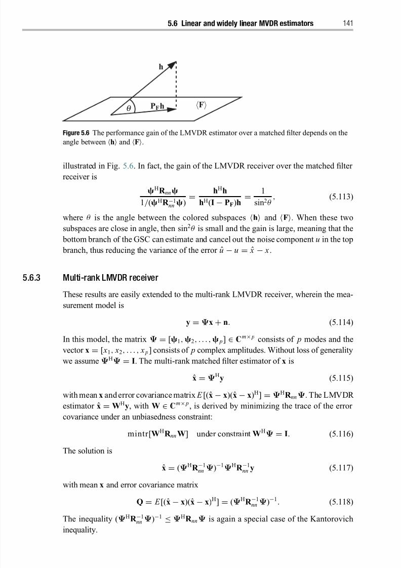
8/21/2019 Statistical Signal Processing of Complex-Valued Data.pdf
http://slidepdf.com/reader/full/statistical-signal-processing-of-complex-valued-datapdf 163/330
5.6 Linear and widely linear MVDR estimators 141
q PFh F
h
Figure 5.6 The performance gain of the LMVDR estimator over a matched filter depends on the
angle between h and F.
illustrated in Fig. 5.6. In fact, the gain of the LMVDR receiver over the matched filter
receiver is
HR nn
1/(HR −1nn ) =
hHh
hH(I − PF)h =1
sin2θ , (5.113)
where θ is the angle between the colored subspaces h and F. When these two
subspaces are close in angle, then sin2θ is small and the gain is large, meaning that the
bottom branch of the GSC can estimate and cancel out the noise component u in the top
branch, thus reducing the variance of the error u − u = ˆ x − x .
5.6.3 Multi-rank LMVDR receiver
These results are easily extended to the multi-rank LMVDR receiver, wherein the mea-surement model is
y =Ψx + n. (5.114)
In this model, the matrix Ψ = [1, 2, . . . , p] ∈ Cm× p consists of p modes and the
vector x = [ x1, x2, . . . , x p] consists of p complex amplitudes. Without loss of generality
we assumeΨHΨ = I. The multi-rank matched filter estimator of x is
x = ΨHy (5.115)
with mean x and error covariance matrix E [(x − x)(x − x)H
] = ΨH
R nnΨ
. The LMVDR estimator x = WHy, with W ∈ Cm× p, is derived by minimizing the trace of the error
covariance under an unbiasedness constraint:
mintr[WHR nn W] under constraint WHΨ = I. (5.116)
The solution is
x = (ΨHR −1nn Ψ)−1
ΨHR −1
nn y (5.117)
with mean x and error covariance matrix
Q = E [(x − x)(x − x)H] = (ΨHR −1nn Ψ)−1. (5.118)
The inequality (ΨHR −1nn Ψ)−1 ≤ΨHR nnΨ is again a special case of the Kantorovich
inequality.
8/21/2019 Statistical Signal Processing of Complex-Valued Data.pdf
http://slidepdf.com/reader/full/statistical-signal-processing-of-complex-valued-datapdf 164/330
142 Estimation
Generalized sidelobe canceler
As in the one-dimensional case, there is a generalized sidelobe-canceler (GSC) struc-
ture. Figure 5.5 still holds, with the one-dimensional matched filter of the top branch
relabeled with the p-dimensional matched filter ΨH and the bottom GSC branch labeled
with the (m − p)-dimensional sidelobe canceler GH, G ∈ Cm×(m− p), where the matrix
U = [Ψ, G] is unitary. The filter connecting the bottom branch to the top branch is
ΨHR nn G(GHR nn G)−1v and the resulting LMVDR estimator of x is the difference
between x + u and u, namely x = x + (u − u) = (x + u) − u:
x = ΨH[I − R nn G(GHR nn G)−1GH]y. (5.119)
From the orthogonality of Ψ and G, it follows that this estimator is unbiased. Moreover,
its variance is the mean-squared error between u and u:
Q = E [(x − x)(x − x)H] = E [(u − u)(u − u)H]
= ΨHR nnΨ−ΨHR nn G(GHR nn G)−1GHR nnΨ = HH(I − PF)H. (5.120)
Here, H = R H/2nn Ψ and F = R H/2
nn G. As in the one-dimensional case, this result produces
the following identity for the error covariance matrix of the LMVDR receiver:
Q = (ΨHR −1nn Ψ)−1 = HH(I − PF)H. (5.121)
The virtue of this identity is that it shows the error covariance to depend on the principal
angles between the subspaces H and F. Figure 5.6 applies correspondingly, if one
accounts for the fact that H is now multidimensional. The gain of the multi-rank LMVDR receiver over the multi-rank matched filter receiver may be written as
det(HHH)
det[HH(I − PF)H] = 1
pi=1
sin2θ i
, (5.122)
where the θ i are the principal angles between the two subspaces H and F. When
these angles are small, the gain is large, meaning that the bottom branch of the GSC
can estimate and cancel out the noise component u in the top branch, thus reducing the
variance of the error u − u.
5.6.4 Subspace identification for beamforming and spectrum analysis
Often the measurement model y = x + n is hypothesized, but the channel vector
that carries the unknown complex parameter x to the measurement is unknown. This
kind of model is called a separable linear model . Call the true unknown vector 0.
A standard ploy in subspace identification, spectrum analysis, and beamforming is to
scan the LMVDR estimator ˆ x through candidates for 0 and choose the candidate that
best models the measurement y. That is to say, the weighted squared error betweenthe measurement y and its prediction ˆ x is evaluated for each candidate and the
minimizing candidate is taken to be the best estimate of 0. Such scanners are called
goniometers. This minimizing candidate is actually the maximum-likelihood estimate
8/21/2019 Statistical Signal Processing of Complex-Valued Data.pdf
http://slidepdf.com/reader/full/statistical-signal-processing-of-complex-valued-datapdf 165/330
5.6 Linear and widely linear MVDR estimators 143
in a multivariate Gaussian model for the noise and it is also the weighted least-squared
error estimate, as we now demonstrate.
Recall that the LMVDR estimate of the complex amplitude x in the measurement
model y=
x +
n is ˆ x =
(HR −
1
nn)
−1HR
−1
nn y. The corresponding LMVDR estima-
tor of the whitened noise R −1/2nn n is R −1/2
nn n = R −1/2nn (y − ˆ x). It is just a few steps of
algebra to write this estimator as
R −1/2nn n = (I − P)w, (5.123)
where w = R −1/2nn y is a whitenedversion of the measurement, = R −1/2
nn is a whitened
version of , and P = (H)−1H is the orthogonal projector onto the subspace
. The mean value of R −1/2nn n is the bias
b
= E [R −1/2
nn n]
=(I
−P)0 x , (5.124)
with 0 = R −1/2nn 0, and its covariance is E [(R −1/2
nn n − b)(R −1/2nn n − b)H] = (I − P).
Thus the bias is zero when = 0, as expected.
The output power of the goniometer is the quadratic form
nHR −1nn n = wH(I − P)w = yHR −1
nn y − H| ˆ x |2 = yHR −1nn y − |HR −1
nn y|2HR −1
nn . (5.125)
This is a biased estimator of the noise-free squared bias bHb:
E (nHR −1
nn
n)=
tr (I−
P)+
bHb=
(m−
1)+
bHb
= (m − 1) + | x|2H0 (I − P)0. (5.126)
At the true value of the parameter 0 the mean value of the goniometer, or maximum-
likelihood function, is m − 1. At other values of the mean value is (m − 1) + bHb. So
the output power of the goniometer is scanned through candidate values of to search
for a minimum.
On the right-hand side of (5.125), only the second term depends on . So a reasonable
strategy for approximating the goniometer is to compute this second term, which is
sometimes called the noncoherent adaptive matched filter . When is a DFT vector, the
adaptive matched filter is a spectrum analyzer or beamformer .5
5.6.5 Extension to WLMVDR receiver
Let us now extend the results for multi-rank LMVDR estimators to multi-rank
WLMVDR estimators that account for complementary covariance.6 The multi-rank
measurement model (5.114) in augmented form is
y = Ψ x + n, (5.127)
where
Ψ =Ψ 0
0 Ψ∗
(5.128)
8/21/2019 Statistical Signal Processing of Complex-Valued Data.pdf
http://slidepdf.com/reader/full/statistical-signal-processing-of-complex-valued-datapdf 166/330
144 Estimation
and the noise n is generally improper with augmented covariance matrix R nn . The
matched filter estimator of x, however, does not take into account noise, and thus the
widely linear matched filter solution is still the linear solution (5.115)
x = ΨHy ⇐⇒ x = ΨHy. (5.129)
The whitened matched filter or WLMVDR estimator, on the other hand, is obtained
as the solution to
mintr[WHR nn W] under constraint WHΨ = I (5.130)
with
W =
W1 W2
W∗2 W∗
1
. (5.131)
This solution is widely linear,
x = (ΨHR −1nn Ψ)−1
ΨHR −1
nn y, (5.132)
with mean x and augmented error covariance matrix
Q = E [(x − x)(x − x)H] = (ΨHR −1nn Ψ)−1. (5.133)
It requires a few steps of algebra to show that the variance of the WLMVDR estimator is
indeed less than or equal to the variance of the LMVDR estimator. Alternatively, we can
argue as follows. The optimization (5.130) is performed under the constraint WHΨ
=I,
or, equivalently, WH1Ψ = I and WH2Ψ = 0. Thus, the WLMMSE optimization prob-lem contains the LMMSE optimization problem as a special case in which W2 = 0
is enforced. Hence, WLMVDR estimation cannot be worse than LMVDR estimation.
However, the additional degree of freedom of being able to choose W2 = 0 can reduce
the variance if the noise n is improper. The results from the preceding subsections –
for instance, the generalized sidelobe canceler – apply in a straightforward manner to
WLMVDR estimation.
The reduction in variance of the WLMVDR compared with the LMVDR estimator
is entirely due to exploiting the complementary correlation of the noise n. Indeed, it is
easy to see that, for proper noise n, the WLMVDR solution (5.132) simplifies to theLMVDR solution (5.117). Since x is not assigned statistical properties, the solution is
independent of whether or not x is improper. This stands in marked contrast to the case
of WLMMSE estimation discussed in Section 5.4.
5.7 Widely linear-quadratic estimation
While widely linear estimation is optimum in the Gaussian case, it may be improved
upon for non-Gaussian data if we have access to higher-order statistics. The next logicalextension of widely linear processing is to widely linear-quadratic (WLQ) processing,
which requires statistical information up to fourth order.7 Because we would like to
keep the notation simple, we shall restrict our attention to systems with vector-valued
input but scalar output.
8/21/2019 Statistical Signal Processing of Complex-Valued Data.pdf
http://slidepdf.com/reader/full/statistical-signal-processing-of-complex-valued-datapdf 167/330
5.7 Widely linear-quadratic estimation 145
5.7.1 Connection between real and complex quadratic forms
What does the most general widely quadratic transformation look like? To answer this
question, we begin with the real-valued quadratic form
u = wTMw, (5.134)
wT = aT bT
, (5.135)
M =
M11 M12
M21 M22
=
M11 M12
MT12 M22
, (5.136)
with u ∈ IR, a, b ∈ IR m , and M11, M12, M21, M22 ∈ IR m×m . Without loss of generality,
we may assume that M is symmetric, and therefore M11 = MT11, M21 = MT
12, and M22 =MT
22. Using
T =I jI
I − jI
, TTH = THT = 2I, (5.137)
the complex version of this real-valued quadratic form is
u = 12(wTTH)
12
TMTH(Tw) = 1
2yHN y (5.138)
with y = a + jb and y = Tw. There is the familiar connection
N
= 12
TMTH
= N1 N2
N∗2 N∗1, (5.139)
N1 = 12[M11 + M22 + j(MT
12 − M12)], (5.140)
N2 = 12[M11 − M22 + j(MT
12 + M12)], (5.141)
and N ∈W m×m is an augmented Hermitian matrix, i.e., NH1 = N1 and NT
2 = N2. In
general, N does not have to be positive or negative (semi)definite. However, if it is, N
will have the same definiteness property as M. Because of the special structure of N, the
quadratic form can be expressed as
u = 1
2 [yH
N1y + yT
N∗1y∗ + yT
N∗2y + yH
N2y∗]
= yHN1y + Re (yHN2y∗). (5.142)
So far, we have considered only a quadratic system with real output u. We may combine
two quadratic systems Nr and Ni to produce the real and imaginary parts, respectively,
of a complex-valued quadratic form:
x = u + jv = 12[yHNr y + jyHNiy] = 1
2yH(Nr + jNi)y. (5.143)
The resulting
H = H11 H12
H21 H22
= Nr + jNi =Nr ,1 + jNi,1 Nr ,2 + jNi,2
N∗r ,2 + jN∗
i,2 N∗r ,1 + jN∗
i,1
(5.144)
no longer has the block pattern of an augmented matrix, i.e., H ∈W m×m , nor is it
generally Hermitian. It does, however, satisfy H22 = HT11, H12 = HT
12, and H21 = HT21.
8/21/2019 Statistical Signal Processing of Complex-Valued Data.pdf
http://slidepdf.com/reader/full/statistical-signal-processing-of-complex-valued-datapdf 168/330
146 Estimation
Thus, a general complex-valued quadratic form can be written as
x = 12
yHHy = 12[yHH11y + yTHT
11y∗ + yTH21y + yHH12y∗]
= y
H
H11y + 1
2 [y
T
H21y + y
H
H12y∗]. (5.145)Combining our results so far, the complex-valued output of a WLQ system can be
expressed as
x = c + 12
gHy + 12
yHHy
= c + 12[gH
1 y + gH2 y∗] + yHH11y + 1
2[yTH21y + yHH12y∗], (5.146)
where c is a complex constant, and gHy with gH = [gH1 , gH
2 ] ∈ C2m constitutes the widely
linear part and yHH y the widely quadratic part.
If x is real, then g1 = g∗2, i.e., g
H
= g
H
1 = [g
H
1 , g
T
1 ] ∈ C
2m
∗ has the structure of anaugmented vector, and H11 = HH11, H21 = H∗
12, i.e., H has the structure of an augmented
matrix (where N1 = H11 and N2 = H12). Thus, for real x ,
x = u = c + 12
gH
1y + 1
2yHN y
= c + Re(gH1 y) + yHN1y + Re(yHN2y∗). (5.147)
We may consider a pair [g, H] to be a vector in a linear space,8 with addition defined by
[g, H] + [g, H] = [g + g, H + H] (5.148)
and multiplication by a complex scalar a by
a[g, H] = [ag, aH]. (5.149)
The inner product in this space is defined by[g, H], [g, H]
= gHg + tr(HHH). (5.150)
5.7.2 WLQMMSE estimation
We would now like to estimate a scalar complex signal x : −→
C from a measurement
y: −→ Cm , using the WLQ estimator
ˆ x = c + gHy + yHHy. (5.151)
For convenience, we have absorbed the factors of 1/2 in (5.146) into g ∈ C2m and
H ∈ C2m×2m . We derive the WLQ estimator as a fairly straightforward extension of
Picinbono and Duvaut (1988) to the complex noncircular case, which avoids the use of
tensor notation. We assume that both x and y have zero mean. In order to ensure that ˆ x
has zero mean as well, we need to choose c = −tr (R yy H) so that
ˆ x = gH
y + yH
Hy − tr (R yy H). (5.152)
Using the definition of the inner product (5.150), the estimator is
ˆ x = [g, HH], [y, y yH − R yy ]
. (5.153)
8/21/2019 Statistical Signal Processing of Complex-Valued Data.pdf
http://slidepdf.com/reader/full/statistical-signal-processing-of-complex-valued-datapdf 169/330
5.7 Widely linear-quadratic estimation 147
In order to make ˆ x a WLQ minimum mean-squared error (WLQMMSE) estimator that
minimizes E | ˆ x − x |2, we apply the orthogonality principle of Result 5.2. That is,
( ˆ x
− x)
⊥ ˆ x , (5.154)
where
ˆ x = gHy + yHHy − tr (R yy H) (5.155)
is any WLQ estimator with arbitrary [g, H]. The orthogonality in (5.154) can be
expressed as
E {( ˆ x − x)∗ ˆ x } = 0, for all g and H. (5.156)
We now obtain
E ( x∗ ˆ x ) = E ( x∗gHy) + E ( x∗yHHy) − E ( x∗)tr(R yy H), (5.157)
and, because x has zero mean,
E ( x∗ ˆ x ) = gH E ( x∗y) + tr [H E ( x∗y yH)]
=
[g, HH], [ E ( x∗y), E ( x∗y yH)]
. (5.158)
Because y has zero mean, we find
E ( ˆ x ˆ x∗) = gH E
ygTy∗ + y yTH∗y∗
+ E
yHHygTy∗ + yHHy yTH∗y∗ − yHHy tr (R ∗ yy H∗)
. (5.159)
By repeatedly using the permutation property of the trace, tr (AB) = tr (BA), we obtain
E ( ˆ x ˆ x∗) = gH E
ygTy∗ + y yTH∗y∗
+ tr
H E (ygTy∗yH + y yTH∗y∗yH − tr (R ∗ yy H∗)y yH)
= [g, HH], [R yy g + E (y yTH∗y∗),
E (y yHyHg) + E (y yH yTH∗y∗) − tr (R ∗ yy H∗)R yy ]
(5.160)
=
[g, HH],K[g, H]
. (5.161)
In the last equation, we have introduced the positive definite operator K, which is defined
in terms of the second-, third-, and fourth-order moments of y. It acts on [g, H] as in
(5.160). We can find an explicit expression for this. Let yi, i
=1, . . . , 2m, denote the
i th element of y, i.e., yi = yi , i = 1, . . . , m, and yi = y∗i−m , i = m + 1, . . . , 2m. Alsolet (R yy )i j denote the (i, j )th element of R yy and (R yy )i the i th row of R yy . Then
K[g, H] = [p, N] (5.162)
8/21/2019 Statistical Signal Processing of Complex-Valued Data.pdf
http://slidepdf.com/reader/full/statistical-signal-processing-of-complex-valued-datapdf 170/330
148 Estimation
with
pi = (R yy )i g +2m
k =
1
2m
l =
1
E ( yi y
k y∗
l ) H ∗kl , i = 1, . . . , 2m,
N i j =2m
k =1
E ( yi y∗
j y∗
k ) g k +
2mk =1
2ml =1
E ( yi y∗
j y
k y∗
l ) H ∗kl
− tr (R ∗ yy H∗)(R yy )i j , i, j = 1, . . . , 2m
=2m
k =1
E ( yi y∗
j y∗
k ) g k +
2mk =1
2ml =1
[ E ( yi y∗
j y
k y∗
l ) − E ( y
i y∗
j ) E ( y
k y∗
l )] H ∗kl . (5.163)
Putting all the pieces together, (5.156) becomes
[g, HH],K[g, H] − [ E ( x∗y), E ( x∗y yH)] = 0. (5.164)
Since this must hold for all g and H, this implies
K[g, H] − [ E ( x∗y), E ( x∗y yH)] = 0, (5.165)
[g, H] = K−1[ E ( x∗y), E ( x∗y yH)]. (5.166)
The MSE achieved by this WLQMMSE estimator is
E | ˆ x − x |2 = E | x |2 − [ E ( x∗y), E ( x∗y yH)], [g, H]= E | x |2 − [ E ( x∗y), E ( x∗y yH)],K−1[ E ( x∗y), E ( x∗y yH)]. (5.167)
Two remarks are in order. First, the widely linear part g of a WLQMMSE filter is not
the WLMMSE filter determined in Result 5.3. Second, it is worth pointing out that the
WLQMMSE filter depends on the complete statistical information up to fourth order.
That is, all conjugation patterns of the second-, third-, and fourth-order moments are
required.
Example 5.4. Consider, for instance, the third-order moments. The formula (5.163)
implicitly utilizes all eight conjugation patterns E ( yi y j yk ), E ( y∗i y j yk ), E ( yi y∗ j yk ),
E ( yi y j y∗k ), E ( y∗i y∗ j yk ), E ( y∗i y j y
∗k ), E ( yi y
∗ j y
∗k ), and E ( y∗i y∗ j y
∗k ). Of course, only two
of these eight conjugation patterns are distinct, due to permutation, e.g., E ( y∗i y j yk ) = E ( y j yk y
∗i ), or complex conjugation, e.g., E ( yi y
∗ j yk ) = [ E ( y∗i y j y
∗k )]
∗.
We may consider E ( yi y
j y
k ) with i, j , k = 1, . . . , 2m as a 2m × 2m × 2m array, more
precisely called a tensor of order 3. This tensor is depicted in Fig. 5.7, and it has many
symmetry relationships. Each m × m × m cube is the complex conjugate of the cube
with which it does not share a side or edge.
A common linear estimation scenario is the estimation of a signal in second-
order white (and proper) noise n whose augmented covariance matrix is R nn = I. For
WLQMMSE estimation, we need to know statistical properties of the noise up to fourth
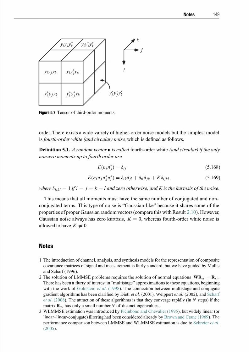
8/21/2019 Statistical Signal Processing of Complex-Valued Data.pdf
http://slidepdf.com/reader/full/statistical-signal-processing-of-complex-valued-datapdf 171/330
Notes 149
j
y∗i y∗ j y∗k
yi y∗ j y∗k yi y j y
∗k
yi y∗ j yk
y∗i y∗ j yk y∗i y j yk
yi y j yk i
k
Figure 5.7 Tensor of third-order moments.
order. There exists a wide variety of higher-order noise models but the simplest model
is fourth-order white (and circular) noise, which is defined as follows.
Definition 5.1. A random vector n is called fourth-order white (and circular) if the only
nonzero moments up to fourth order are
E (ni n∗ j ) = δi j (5.168)
E (ni n j n∗k n
∗l ) = δi k δ jl + δil δ j k + K δi j k l , (5.169)
where δi j k l = 1 if i = j = k = l and zero otherwise, and K is the kurtosis of the noise.
This means that all moments must have the same number of conjugated and non-
conjugated terms. This type of noise is “Gaussian-like” because it shares some of the
properties of proper Gaussian random vectors (compare this with Result 2.10). However,
Gaussian noise always has zero kurtosis, K = 0, whereas fourth-order white noise is
allowed to have K = 0.
Notes
1 The introduction of channel, analysis, and synthesis models for the representation of composite
covariance matrices of signal and measurement is fairly standard, but we have guided by Mullis
and Scharf (1996).
2 The solution of LMMSE problems requires the solution of normal equations WR yy = R x y .
There has been a flurry of interest in “multistage” approximations to these equations, beginning
with the work of Goldstein et al . (1998). The connection between multistage and conjugate
gradient algorithms has been clarified by Dietl et al. (2001), Weippert et al. (2002), and Scharf
et al . (2008). The attraction of these algorithms is that they converge rapidly (in N steps) if the
matrix R yy
has only a small number N of distinct eigenvalues.
3 WLMMSE estimation was introduced by Picinbono and Chevalier (1995), but widely linear (or
linear–linear-conjugate) filtering had been considered already by Brown and Crane (1969). The
perfor mance comparison between LMMSE and WLMMSE estimation is due to Schreier et al .
(2005).

8/21/2019 Statistical Signal Processing of Complex-Valued Data.pdf
http://slidepdf.com/reader/full/statistical-signal-processing-of-complex-valued-datapdf 172/330
150 Estimation
4 Our discussionof reduced-rank estimators follows Scharf (1991), Hua et al . (2001),and Schreier
and Scharf (2003a). Canonical coordinate systems are optimum even for the more general
problem of transform coding for noisy sour ces (under some restrictive assumptions), which has
been shown by Schreier and Scharf (2006a). This, however, is not considered in this chapter.
5 There are many variations on the goniometer that aim to adapt to unknown noise covariance.They go by the name “adaptive beamforming” or “Capon beamforming,” after Jack Capon,
who first advocated alternatives to conventional beamforming. Capon applied his methods to
the processing of multi-sensor array measurements.
6 The WLMVDR receiver was introduced by McWhorter and Schreier (2003), where it was
applied to widely linear beamforming, and then analyzed in mor e detail by Chevalier and Blin
(2007).
7 Widely linear-quadraticsystems fordetectionand array processing were introduced byChevalier
and Picinbono (1996).
8 The linear space consisting of vectors [g, H] is the direct sum of the Hilbert spaces C 2m and
C2m×2m , usually denoted as C2m
⊕C2m×2m .
8/21/2019 Statistical Signal Processing of Complex-Valued Data.pdf
http://slidepdf.com/reader/full/statistical-signal-processing-of-complex-valued-datapdf 173/330
6 Performance bounds forparameter estimation
All parameter estimation begins with a measurement and an algorithm for extracting a
parameter estimate from the measurement. The algorithm is the estimator.
There are two ways to think about performance analysis. One way is to begin with a
particular estimator and then to compute its performance. Typically this would amount
to computing the bias of the estimator and its error covariance matrix. The practitioner
then draws or analyzes concentration ellipsoids to decide whether or not the estimator
meets specifications. But the other, more general, way is to establish a limit on the
accuracy of any estimator of the parameter. We might call this a uniform limit, uniform
over an entire class of estimators. Such a limit would speak to the information that
the measurement carries about the underlying parameter, independently of how the
information is extracted.
Performance bounds are fundamental to signal processing because they tell us when
the number and quality of spatial, temporal, or spatial–temporal measurements is suf-
ficient to meet performance specifications. That is, these general bounds speak to the
quality of the experiment or the sensing schema itself, rather than to the subsequent
signal processing. If the sensing scheme carries insufficient information about the
underlying parameter, then no amount of sophisticated signal processing can extract
information that is not there. In other words, if the bound says that the error covariance
is larger than specifications require, then theexperiment or measurement schememust be
redesigned.
But there is a cautionary note here: the performance bounds we will derive are
lower bounds on variance, covariance, and mean-squared error. They are not nec-essarily tight. So, even if the bound is smaller than specifications require, there
is still no guarantee that you will be able to find an estimator that achieves this
bound. So the bound may meet variance specifications, but your estimator might
not. Peter Schultheiss has called performance bounds spoiled-sport results because
they establish unwelcome limits on what can be achieved and because they can
be used to bring into question performance claims that violate these fundamental
bounds.
In this book, measurements are complex-valued and parameters are complex-valued.
So the problem is to extract an estimate of a complex parameter from a complexmeasurement. As we have seen in previous chapters, we need to consider the correlation
structure for errors and measurements and their complex conjugates, since this enables
us to account for complementary correlation.
8/21/2019 Statistical Signal Processing of Complex-Valued Data.pdf
http://slidepdf.com/reader/full/statistical-signal-processing-of-complex-valued-datapdf 174/330
152 Performance bounds for parameter estimation
In this chapter, we shall consider quadratic performance bound s of the Weiss–
Weinstein class, which were introduced by Weiss and Weinstein (1985). The idea behind
this class of bounds is to establish a lower bound on the error covariance for a parameter
estimator by considering an approximation of the estimator error from a linear function
of a score function. This is very sophisticated reasoning: “If I use a linear function
of a score function to approximate the estimator error, then maybe I can use the error
covariance of this approximation to derive a bound on the error covariance for any esti-
mator.” Of course, the bound will depend on the score function that is chosen for the
approximation. The idea is then to choose good scores, and among these are the Fisher,
Bhattacharyya, Ziv–Zakai, Barankin, and Bobrovsky–Zakai scores. In our extension of
this reasoning, we will approximate the error using a widely linear function of the score
function.
We shall develop a frequentist theory of quadratic performance bounding and a
Bayesian theory. Frequentist bounds are sometimes called deterministic bounds and
Bayesian boundsare sometimescalled stochastic bounds.For a frequentist the underlying
assumption is that an experiment produces a measurement y that is drawn from a
distribution P (y). The parameter of this distribution is unknown, and to be estimated.
Repeated trials of the experiment would consist of repeated draws of the measurements
{yi} from the same distribution, with fixed. For a Bayesian the underlying assumption
is that a random parameter and a random measurement (y, ) are drawn from a joint
distribution P (y, ). Repeated trials of the experiment would consist of repeated draws
of the measurement and parameter pairs (
{yi
}, ), with the parameter a single, fixed,
random draw. In some cases the repeated draws are ({yi , i}). For the frequentist and
the Bayesian there is a density for the measurement, indexed by the parameter, but for
the Bayesian there is also a prior distribution that may concentrate the probability of the
parameter. For the frequentist there is none.1
The organization of this chapter is as follows. Section 6.1 introduces the frequen-
tist and Bayesian concepts and establishes notation. Section 6.2 discusses quadratic
frequentist bounds in general, and Section 6.3 presents the most common frequentist
bound, the Cramer–Rao bound. Bayesian bounds are investigated in Section 6.4, and
the best-known Bayesian bound, the Fisher–Bayes bound (or “stochastic Cramer–Rao
bound”), is derived in Section 6.5. When these bounds are specialized to the multivariateGaussian model, then the formulae of this chapter reproduce or generalize those of a
great number of authors who have computed quadratic bounds for spectrum analysis
and beamforming. Finally, Section 6.6 establishes connections and orderings among the
bounds.
6.1 Frequentists and Bayesians
Frequentists model the complex measurement as a random vector y: −→ Cn
with probability distribution P (y) andprobabilitydensity function (pdf) p(y). These depend
on the parameter , which is unknown but known to belong to the set Θ ⊆ C p. As
explained in Section 2.3, the probability distribution and pdf of a complex random
8/21/2019 Statistical Signal Processing of Complex-Valued Data.pdf
http://slidepdf.com/reader/full/statistical-signal-processing-of-complex-valued-datapdf 175/330
6.1 Frequentists and Bayesians 153
vector are interpreted as the joint distribution and pdf of its real and imaginary parts.
Typically, and throughout this chapter, the random vector y is continuous. If y contains
discrete components, the pdf can be expressed using Dirac δ-functions.
Bayesians regard both the measurement y: −→
Cn and the parameter : −→
C p
as random vectors defined on the same sample space. They are given a joint probability
distribution P (y, ), and pdf p(y, ). The joint pdf may be expressed as
p(y, ) = p(y) p(), (6.1)
where p(y) = p(y|) is the conditional measurement pdf and p() is the prior pdf on
the random parameter .
So, when is deterministic, p(y) denotes a parameterized pdf. When it is random,
p(y) denotes a conditional pdf. We do not make any distinction in our notation, since
context clarifies which meaning is to be taken.
In our development of performance bounds on estimators of the parameter we
will construct error scores and measurement scores. These are functions of the mea-
surement or of the measurement and parameter. Moreover, later on we shall augment
these with their complex conjugates so that we can construct bounds based on widely
linear estimates of error scores from measurement scores. We work with the space of
square-integrable measurable functions (i.e., their Hermitian second-order moments are
finite) of the complex random vector y, or of the complex random vector (y, ), and
assume all errors and scores to be elements of this space. Of course, a finite Hermitian
second-order moment ensures a finite complementary second-order moment.
Definition 6.1. Throughout this chapter we define Cn
f (y)d y
IR 2n
Re[f (y)]d[Re y]d[Im y] + j
IR 2n
Im[f (y)]d[Re y]d[Im y]. (6.2)
That is, an integral with respect to a complex variable is the integral with respect to its
real and imaginary parts.
The mean value of any function g(y), computed with respect to the parameterized pdf
p(y), is
E [g(y)] = Cn
g(y) p(y)d y. (6.3)
The mean value of any function g(y, ), computed with respect to the joint pdf p(y, ),
is
E [g(y, )] =
C p×Cn
g(y, ) p(y, )d y d
=
C p
Cn
g(y, ) p(y)d y
p()d
= E { E [g(y, )]}. (6.4)
In this notation, E [g(y, )] is a conditional expectation with respect to the conditional
pdf p(y), and the outer E is the expectation over the distribution of .
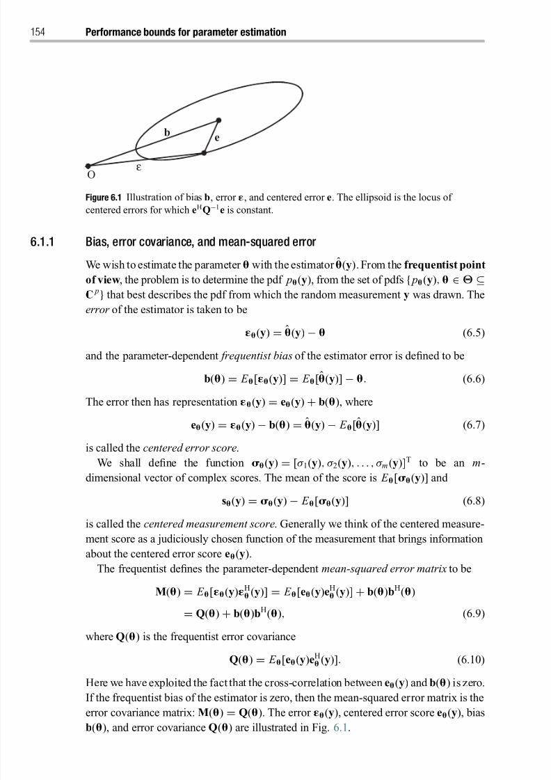
8/21/2019 Statistical Signal Processing of Complex-Valued Data.pdf
http://slidepdf.com/reader/full/statistical-signal-processing-of-complex-valued-datapdf 176/330
154 Performance bounds for parameter estimation
b
O ε
e
Figure 6.1 Illustration of bias b, error , and centered error e. The ellipsoid is the locus of
centered errors for which eHQ−1e is constant.
6.1.1 Bias, error covariance, and mean-squared error
We wish to estimate the parameter with the estimator (y). From the frequentist point
of view, the problem is to determine the pdf p(y), from the set of pdfs { p(y), ∈Θ ⊆C p} that best describes the pdf from which the random measurement y was drawn. The
error of the estimator is taken to be
(y) = (y) − (6.5)
and the parameter-dependent frequentist bias of the estimator error is defined to be
b() = E [(y)] = E [(y)] − . (6.6)
The error then has representation (y)=
e(y)+
b(), where
e(y) = (y) − b() = (y) − E [(y)] (6.7)
is called the centered error score.
We shall define the function (y) = [σ 1(y), σ 2(y), . . . , σ m(y)]T to be an m-
dimensional vector of complex scores. The mean of the score is E [(y)] and
s(y) = (y) − E [(y)] (6.8)
is called the centered measurement score. Generally we think of the centered measure-
ment score as a judiciously chosen function of the measurement that brings information
about the centered error score e(y).
The frequentist defines the parameter-dependent mean-squared error matrix to be
M() = E [(y)H (y)] = E [e(y)eH
(y)] + b()bH()
= Q() + b()bH(), (6.9)
where Q() is the frequentist error covariance
Q() = E [e(y)eH (y)]. (6.10)
Here we have exploited the fact that the cross-correlation between e(y) and b() is zero.If the frequentist bias of the estimator is zero, then the mean-squared error matrix is the
error covariance matrix: M() = Q(). The error (y), centered error score e(y), bias
b(), and error covariance Q() are illustrated in Fig. 6.1.
8/21/2019 Statistical Signal Processing of Complex-Valued Data.pdf
http://slidepdf.com/reader/full/statistical-signal-processing-of-complex-valued-datapdf 177/330
6.1 Frequentists and Bayesians 155
From the Bayesian point of view, we wish to determine the joint pdf p(y, ) from
the set of pdfs { p(y, ), ∈Θ ⊆ C p} that best describes the joint pdf from which the
random measurement–parameter pair (y, ) was drawn. The estimator error is
(y, ) = (y) − (6.11)
and the Bayes bias of the estimator error is
b = E [(y, )] = E { E [(y)]} = E [b()] = E [(y)] − E []. (6.12)
The Bayes bias is the average of the frequentist bias because the Bayesian and the
frequentist define their errors in the same way: (y, ) = (y). The error then has the
representation (y, ) = e(y, ) + b, where the centered error score is defined to be
e(y, ) = (y, ) − b = (y) − E [(y)] − ( − E []). (6.13)
The measurement score is defined to be the m-dimensional vector of complex scores
(y, ) = [σ 1(y, ), σ 2(y, ), . . . , σ m(y, )]T. The mean value of the measurement score
is E [(y, )] = E { E [(y, )]} and the centered measurement score is
s(y, ) = (y, ) − E [(y, )]. (6.14)
The mean E [(y, )] is generally not E { E [(y)]} because the Bayesian will define
a score (y, ) that differs from the frequentist score (y), in order to account for
prior information about the parameter . Again we think of scores as judiciously chosen
functions of the measurement that bring information about the true parameter.
The Bayesian defines the mean-squared error matrix for the estimator (y) to be
M = E [(y, )H(y, )] = E { E [(y)H (y)]} = E [M()], which is the average over
the prior distribution on of the frequentist mean-squared error matrix M(). This
average may be written
M = E [(y, )H(y, )] = E [e(y, )eH(y, )] + bbH = Q + bbH, (6.15)
where Q is the Bayes error covariance
Q = E [e(y, )eH(y, )]. (6.16)
Note that the Bayes bias and error covariance matrix are independent of the parameter . If the Bayes bias of the estimator is zero, then the mean-squared error matrix is the
error covariance matrix: M = Q.
6.1.2 Connection between frequentist and Bayesian approaches
We have established that the Bayes bias b = E [b()] is the average of the frequentist
bias and the Bayes mean-squared error matrix M = E [M()] is the average of the
frequentist mean-squared error matrix. But what about the Bayes error covariance Q? Is
it the average over the distribution of the parameter of the frequentist error covarianceQ()? The answer (surprisingly) is no, as the following argument shows.
The Bayesian’s centered error score may be written in terms of the frequentist’s
centered error score as e(y, ) = e(y) + (b() − b). In this representation, e(y) and
8/21/2019 Statistical Signal Processing of Complex-Valued Data.pdf
http://slidepdf.com/reader/full/statistical-signal-processing-of-complex-valued-datapdf 178/330
156 Performance bounds for parameter estimation
b() − b are conditionally and unconditionally uncorrelated, so as a consequence the
Bayesian’s error covariance may be written in terms of the frequentist’s parameter-
dependent error covariance as
Q = E [Q()] + R bb, (6.17)
where R bb = E [(b() − b)(b() − b)H] is the covariance of the parameter-dependent
bias b(). If the frequentist bias of the estimator is constant at b() = b, then R bb = 0
and the Bayes error covariance is the average over the distribution of the param-
eter of the frequentist error covariance. In other words, we have the following
result.
Result 6.1. The frequentist error covariance can be averaged for the Bayes error covari-
ance to produce the identity
Q = E [Q()] (6.18)
if and only if the frequentist bias of the estimator is constant.
This generally is a property of linear minimum-variance distortionless response
(LMVDR) estimators, also called best linear unbiased estimators (BLUEs) – for which
b() = 0 – but not of MMSE estimators. The following example is illuminating.
Example 6.1. Consider the linear signal-plus-noise model
y = H + n, (6.19)
where H ∈ Cn× p, ∈ C p is zero-mean proper Gaussian with covariance matrix R θ θ , n
is zero-mean proper Gaussian with covariance matrix R nn , and and n are independent.
Following Section 5.6, the LMVDR estimator (also called BLUE), which in this case is
also the maximum-likelihood (ML) estimator, is
LMVDR (y) = (HHR −1nn H)−1HHR −1
nn y = + (HHR −1nn H)−1HHR −1
nn n, (6.20)
which ignores the prior distribution on . Consequently the frequentist bias is
b() = 0 and the Bayes bias is b = 0. The centered frequentist error is e(y) =(HHR −1nn H)−1HHR −1
nn n. The frequentist error covariance is then Q() = (HHR −1nn H)−1
and this is also the Bayes error covariance Q:
QLMVDR = (HHR −1nn H)−1 = E [QLMVDR ()] = QLMVDR (). (6.21)
The MMSE estimator accounts for the distribution of :
MMSE(y) = (HHR −1nn H + R −1
θ θ )−1HHR −1
nn y
= (HHR −1nn H + R −1
θ θ )−1HHR −1
nn H + (HHR −1nn H + R −1
θ θ )−1HHR −1
nn n. (6.22)
The frequentist bias of this estimator is b() = (HHR −1nn H + R −1
θθ )−1HHR −1nn H − and the Bayes bias is b = 0. The frequentist error covariance of this estimator is Q() =(HHR −1
nn H + R −1θθ )
−1HHR nn H(HHR −1nn H + R −1
θ θ )−1. The Bayes error covariance is the
sum of the expectation of the frequentist error covariance Q() and the covariance
8/21/2019 Statistical Signal Processing of Complex-Valued Data.pdf
http://slidepdf.com/reader/full/statistical-signal-processing-of-complex-valued-datapdf 179/330
6.2 Quadratic frequentist bounds 157
of the parameter-dependent bias R bb = E [b()bH()]. But, since the frequentist error
covariance is independent of , we may write
QMMSE
=QMMSE()
+R bb
=(HHR −1
nn H
+R −1
θ θ )−1
≤ (HHR −1nn H)−1 = QLMVDR () = QLMVDR . (6.23)
There are lessons here: the MMSE estimator has smaller Bayes error covariance than
the LMVDR estimator; it also has smaller frequentist error covariance. Its only vice is
that it is not frequentist unbiased. So, from the point of view of Bayes error covariance,
frequentist unbiasedness is no virtue. In fact, it is uncommon for the frequentist bias of
an estimator of a random parameter to be zero, but common for the Bayes bias to be
zero.
6.1.3 Extension to augmented errors
These results extend to the characterization of augmented error scores eT = [eT, eH].
The augmented Bayes bias remains the average of the augmented frequentist bias, which
is to say that b = E [b()], the augmented Bayes mean-squared error matrix remains the
average of the augmented frequentist mean-squared error matrix, M = E [M()], and
the Bayes and frequentist augmented error covariances remain related as
Q=
E [Q()]+
R bb
, (6.24)
where Q() = E [e(y)eH(y)] is the augmented frequentist error covariance matrix and
R bb = E [(b() − b)(b() − b)H] is the augmented covariance matrix for the frequentist
bias.
6.2 Quadratic frequentist bounds
Let us begin our discussion of quadratic frequentist covariance bounds by considering
the Hermitian version of the story, where complementary covariances are ignored in the bounding procedure.Then wewill extendtheseboundsbyaccountingfor complementary
covariances and find that this tightens the bounds.
Here is the idea: from the measurement y is computed the estimator (y), with
frequentist error (y) = (y) − and centered error score e(y) = (y) − b(). We
would like to approximate this centered error score by using a linear function of the
centered measurement score s(y).
6.2.1 The virtual two-channel experiment and the quadratic frequentist bound
Consider the virtual two-channel estimation problem of Fig. 6.2, which is reminiscent
of the virtual two-channel problems developed in Section 5.3. In Fig. 6.2, the centered
error score e(y) is to be estimated from the centered measurement score s(y). The first
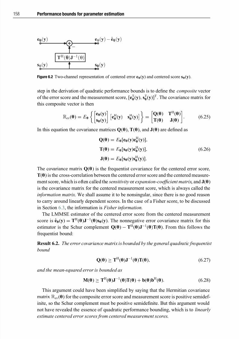
8/21/2019 Statistical Signal Processing of Complex-Valued Data.pdf
http://slidepdf.com/reader/full/statistical-signal-processing-of-complex-valued-datapdf 180/330
158 Performance bounds for parameter estimation
eθθ(y)
sθθ(y)
eθ(y)− eθθ(y)
TH
(θθ)J−1
(θ)sθ(y)
Figure 6.2 Two-channel representation of centered error e(y) and centered score s(y).
step in the derivation of quadratic performance bounds is to define the composite vector
of the error score and the measurement score, [eT(y), sT
(y)]T. The covariance matrix for
this composite vector is then
Res () = E e(y)
s(y) eH
(y) sH
(y) = Q() TH()
T() J() . (6.25)
In this equation the covariance matrices Q(), T(), and J() are defined as
Q() = E [e(y)eH (y)],
T() = E [s(y)eH (y)], (6.26)
J() = E [s(y)sH (y)].
The covariance matrix Q() is the frequentist covariance for the centered error score,
T() is the cross-correlation between the centered error score and the centered measure-
ment score, which is often called the sensitivity or expansion-coefficient matrix, and J()
is the covariance matrix for the centered measurement score, which is always called the
information matrix. We shall assume it to be nonsingular, since there is no good reason
to carry around linearly dependent scores. In the case of a Fisher score, to be discussed
in Section 6.3, the information is Fisher information.
The LMMSE estimator of the centered error score from the centered measurement
score is e(y) = TH()J−1()s(y). The nonnegative error covariance matrix for this
estimator is the Schur complement Q() − TH()J−1()T(). From this follows the
frequentist bound:
Result 6.2. The error covariance matrix is bounded by the general quadratic frequentist
bound
Q() ≥ TH()J−1()T(), (6.27)
and the mean-squared error is bounded as
M() ≥ TH()J−1()T() + b()bH(). (6.28)
This argument could have been simplified by saying that the Hermitian covariance
matrix Res () for the composite error score and measurement score is positive semidef-inite, so the Schur complement must be positive semidefinite. But this argument would
not have revealed the essence of quadratic performance bounding, which is to linearly
estimate centered error scores from centered measurement scores.
8/21/2019 Statistical Signal Processing of Complex-Valued Data.pdf
http://slidepdf.com/reader/full/statistical-signal-processing-of-complex-valued-datapdf 181/330
6.2 Quadratic frequentist bounds 159
As noted by Weinstein and Weiss (1988), the Battacharrya, Ziv–Zakai, Barankin, and
Bobrovsky–Zakai bounds all have this quadratic structure. Only the choice of score
distinguishes one bound from another. Moreover, each quadratic bound is invariant
with respect to nonsingular linear transformation of the score function s. That is, the
transformed score Ls transforms the sensitivity matrix T to LT and the information
matrix J to LJLH, leaving the bound invariant.
Definition 6.2. An estimator is said to be efficient with respect to a given score if the
bound in (6.27) is achieved with equality: Q() = TH()J−1()T().
That is, the estimated error score equals the actual error score:
e(y) = TH()J−1()s(y). (6.29)
This is also invariant with respect to linear transformation L. That is, an estimator isefficient if, element-by-element, its centered error score lies in the subspace spanned by
the elements of the centered measurement score. The corresponding representation for
the estimator itself is (y) − = TH()J−1()s(y).
One score is better than another if its quadratic bound is larger than the other. So the
search goes on for a better bound, or in fact a better score.
Good and bad scores
We shall not give the details here, but McWhorter and Scharf (1993c) showed that a
given measurement score can be improved, in the sense that it improves the quadraticfrequentist bound, by “Rao–Blackwellizing” it. To “Rao–Blackwellize” is to compute
the expected value of the centered measurement score, conditioned on the frequentist
sufficient statistic for the parameter. In other words, to be admissible a score must be a
function of the sufficient statistic for the parameter to be estimated. Moreover, additional
score functions never hurt, which is to say that the quadratic performance bound is never
loosened with the addition of additional scores.
6.2.2 Projection-operator and integral-operator representations of quadratic
frequentist bounds
Let us consider the variance bound for one component of the parameter vector . Call
it θ . The corresponding component of the estimator (y) is called θ (y), and the cor-
responding component of the centered error score is eθ (y) = θ (y) − E [θ (y)]. Without
loss of generality, assume that scores have been transformed into a coordinate sys-
tem where the information matrix is J(θ ) = I. The composite covariance matrix for
[eθ (y), sTθ (y)]T is
Res (θ ) = E eθ (y)
sθ (y) e∗θ (y) sHθ (y) = Q(θ ) tH(θ )
t(θ ) I , (6.30)
where t(θ ) = E [sθ (y)e∗θ (y)] is the m-dimensional column vector of expansion coeffi-
cients in this transformed coordinate system. Then the invariant quadratic frequentist

8/21/2019 Statistical Signal Processing of Complex-Valued Data.pdf
http://slidepdf.com/reader/full/statistical-signal-processing-of-complex-valued-datapdf 182/330
160 Performance bounds for parameter estimation
eq(y)
s1 s2 sm
Figure 6.3 Projection of the error eθ (y) onto the Hilbert space of centered error scores
s1, s2, . . . , sm .
bound may be written
Q(θ ) ≥ tH(θ )t(θ ) =m
i=1
|t i (θ )|2, (6.31)
where t i (θ ) is the i th coordinate of the m-dimensional expansion-coefficient vector t(θ ).
The score random variables are uncorrelated with variance unity, so we may write the
previous equation as
Q(θ ) ≥ E
mi=1
m j =1
t i s∗i t ∗ j s j
= E | s eθ (y)|2, (6.32)
where the operator s eθ (y) acts like this:
s eθ (y) =m
i=1
t ∗i si =m
i=1
E [ s∗i (y)eθ (y)] si (y). (6.33)
This projection operator projects the centered error score eθ (y) onto each element of the
centered measurement score (or onto the Hilbert space of centered measurement scores),
as illustrated in Fig. 6.3. Thus, for the bound (6.31) to be tight, the actual error score
eθ (y) must lie close to the subspace spanned by the m centered measurement scores.
This interpretation makes it easy to see that the elements of the vector t(θ ) are just the
coefficients of the true error eθ (y) in the basis sθ (y). That is, t i (θ ) = E [ si (y)e∗θ (y)].
There is also a kernel representation of this bound due to McWhorter and Scharf
(1993c). Write the projection as
s eθ (y) =m
i=1
t ∗i si =
eθ (y)m
i=1
si (y) s∗i (y) pθ (y)d y
=
eθ (y) K θ (y, y) pθ (y)d y. (6.34)
So, for a tight bound, s eθ (y) must be nearly the actual error eθ (y), which is to say that
the actual error eθ (y) must nearly be an element of the reproducing kernel Hilbert space
defined by the kernel
K θ (y, y) =m
i=1
si (y) s∗i (y). (6.35)
8/21/2019 Statistical Signal Processing of Complex-Valued Data.pdf
http://slidepdf.com/reader/full/statistical-signal-processing-of-complex-valued-datapdf 183/330
6.2 Quadratic frequentist bounds 161
6.2.3 Extension of the quadratic frequentist bound to improper errors and scores
The essential step in the extension of quadratic frequentist bounds to improper error and
measurement scores is to define the composite vector of augmented errors and scores,
[eT, sT]T. The covariance matrix for this composite vector is
E
e(y)
s(y)
eH
(y) sH (y)
=
Q() TH()
T() J()
. (6.36)
In this equation the constituent matrices are defined as
Q() = E [e(y)eH (y)] =
Q() Q()Q∗() Q∗()
,
T() = E [s(y)eH (y)] = T() T()T∗() T∗(), (6.37)
J() = E [s(y)sH (y)] =
J() J()
J∗() J∗()
.
The covariance matrix T() = E [s(y)eT(y)] is the complementary sensitivity or
expansion-coefficient matrix, and J() = E [s(y)sT(y)] is the complementary covari-
ance matrix for the centered measurement score, which is called the complementary
information matrix. Furthermore, Q() is the augmented error covariance matrix, T()
is the augmented sensitivity or expansion-coefficient matrix, and J() is the augmented
information matrix. Obviously, we are interested in bounding Q() rather than Q(),
but it is convenient to derive the bounds on Q() first, from which one can immediately
obtain the bound on Q().
The covariance matrix for the composite vector of augmented error score and aug-
mented measurement score is positive semidefinite, so, assuming the information matrix
to be nonsingular, we obtain the bound Q() ≥ TH()J−1()T(). From this, we can
read out the northwest block of Q() to obtain the following result.
Result 6.3. The frequentist error covariance is bounded as
Q() ≥ TH() TT()
J−1() T()T∗()
. (6.38)
The quadratic form on the right-hand side is the general widely linear-quadratic fre-
quentist bound on the error covariance matrix for improper error and measurement
scores. Of course the underlying idea is that Q() − TH()J−1()T() is the augmented
error covariance matrix of the widely linear estimator of the error score from the mea-
surement score:
e(y)
= TH() TT() J−1()s(y). (6.39)
The bound in Result 6.3 is tighter than the bound in Result 6.2, but for proper mea-
surement scores (i.e., J() = 0) and cross-proper measurement and error scores (i.e.,T() = 0) the bounds are identical.

8/21/2019 Statistical Signal Processing of Complex-Valued Data.pdf
http://slidepdf.com/reader/full/statistical-signal-processing-of-complex-valued-datapdf 184/330
162 Performance bounds for parameter estimation
A widely linear estimator is efficient if equality holds in (6.38). This is the case if and
only if the estimator of the centered error score equals the actual error, meaning that the
estimator has the representation
(y) − = TH() TT() J−1()s(y). (6.40)
6.3 Fisher score and the Cram ´ er–Rao bound
Our results for quadratic frequentist bounds so far are general. To make them applicable
we need to consider a concrete score for which T() and J() can be computed. For this
we choose the Fisher score and compute its associated Cramer–Rao bound.
Definition 6.3. The Fisher score is defined as
(y) =
∂
∂log p(y)
H
=
∂
∂θ ∗1log p(y), . . . ,
∂
∂θ ∗ plog p(y)
T
, (6.41)
where the partial derivatives are Wirtinger derivatives as discussed in Appendix 2.
The i th component of the Fisher score is
σ i (y) = ∂
∂(Re θ i )log p(y) + j
∂
∂(Im θ i )log p(y). (6.42)
Thus, the Fisher score is a p-dimensional complex-valued column vector. The notation(∂/∂) p(y) means (∂/∂ ) p(y), evaluated at = . We shall demonstrate shortly
that the expected value of the Fisher score is E [(y)] = 0, so that Definition 6.3 also
defines the centered measurement score s(y).
The Fisher score has a number of properties that make it a compelling statistic for
inferring the value of a parameter and for bounding the error covariance of any estimator
for that parameter. We list these properties and annotate them here.
1. We may write the partial derivative as
∂
∂θ ∗i log p(y) =1
p(y)
∂
∂θ ∗i p(y), (6.43)
which is a normalized measure of the sensitivity of the pdf p(y) to variations in the
parameter θ i . Large sensitivity is valued, and this will be measured by the variance
of the score.
2. TheFisher score is a zero-mean randomvariable.This statisticalproperty is consistent
with maximum-likelihood procedures that search for maxima of the log-likelihood
function log p(y) by searching for the zeros of (∂/∂)log p(y). Functions with steep
slopes are valued, so we value a zero-mean score with large variance.
3. The cross-correlation between the centered Fisher score and the centered error score
is the expansion-coefficient matrix
T() = I +
∂
∂b()
H
, (6.44)

8/21/2019 Statistical Signal Processing of Complex-Valued Data.pdf
http://slidepdf.com/reader/full/statistical-signal-processing-of-complex-valued-datapdf 185/330
6.3 Fisher score and the Cram´ er–Rao bound 163
where as before b() is the frequentist bias of the estimator. The (i, j )th element of
the matrix (∂/∂)b() is (∂/∂θ j )bi (). When the estimator is unbiased, then T = I,
which is to say that the measurement score is perfectly aligned with the error score.
The effect of bias is to misalign them.
4. The Fisher information matrix is also the expected Hessian of the score function (up
to a minus sign):
JF() = E
∂
∂log p(y)
H∂
∂log p(y)
= − E
∂
∂
∂
∂log p(y)
H
. (6.45)
The first of these four properties is interpretive only. The next three are interpretive
and analytical. Let’s prove them.
2. The expected value of the Fisher score is
E [(y)] =
∂
∂log p(y)
H
p(y)d y =
∂
∂ p(y)
H
d y = 0. (6.46)
3. The frequentist bias b() of the parameter estimator (y) may be differentiated with
respect to as follows:
∂
∂
b()
=∂
∂ [(y)
−] p(y)d y
=
[(y) − ]
∂
∂log p(y)
p(y)d y − I
= E [(y)H (y)] − I = TH() − I. (6.47)
In the last line, we have used E [(y)] = 0.
4. Consider the p × p Hessian matrix
∂
∂ ∂
∂log p(y)
H
= ∂
∂ ∂
∂ p(y)
H1
p(y)
= ∂
∂
∂
∂ p(y)
H1
p(y) −
∂
∂log p(y)
H∂
∂log p(y).
(6.48)
The expectation of this matrix is
E
∂
∂
∂
∂log p(y)
H= 0 − E [s(y)sH
(y)] = −JF(). (6.49)
Result 6.4. The quadratic frequentist bound for the Fisher score is the Cram er–Raobound:
Q() ≥
I + ∂
∂b()
J−1
F ()
I + ∂
∂b()
H
. (6.50)
8/21/2019 Statistical Signal Processing of Complex-Valued Data.pdf
http://slidepdf.com/reader/full/statistical-signal-processing-of-complex-valued-datapdf 186/330
164 Performance bounds for parameter estimation
When the frequentist bias is zero, then the Cram´ er–Rao bound is
Q() ≥ J1F(), (6.51)
where JF() is the Fisher information.This bound is sometimes also called the deterministic Cramer–Rao bound, in order to
differentiate it from the corresponding Bayesian (i.e., stochastic) bound in Result 6.7. It
is the most celebrated of all quadratic frequentist bounds.
If repeated measurements carry information about one fixed and deterministic param-
eter through the product pdf M
i=1 p(yi ), then the sensitivity matrix remains fixed
and the Fisher information matrix scales with M . Consequently the Cramer–Rao bound
decreases as M −1.
6.3.1 Nuisance parameters
There are many ways to show the effect of nuisance parameters on error bounds, and
some of these are given by Scharf (1991, pp. 231–233). But perhaps the easiest, if
not most general, way to establish the effect is this. Begin with the Fisher informa-
tion matrix J() and the corresponding Cramer–Rao bound for frequentist unbiased
estimators, Q() ≥ J−1(). (In order to simplify the notation we do not subscript J as
JF.) The (i, i)th element of J() is J i i () and the (i, i )th element of J−1() is denoted
by (J−1)ii ().
From the definition of a score we see that J ii () is the Fisher information for the i thelement of , when only the i th parameter in the parameter vector is unknown.
The Cauchy–Schwarz inequality says that (yHJy)(xHJx) ≥ |yHJx|2. Choose x = uk
and y = J−1uk , with uk the k th Euclidean basis vector. Then (J−1)ii () J i i () ≥ 1,
or (J−1)ii () ≥ 1/ J ii (). These results actually generalize to show that any r -by-r -
dimensional submatrix of the p-by- p inverse J−1() is more positive definite than the
inverse of the corresponding r -by-r Fisher matrix J(). So nuisance parameters increase
the Cramer–Rao bound.
6.3.2 The Cram ´ er–Rao bound in the proper multivariateGaussian model
In Result 2.5, the pdf for a proper complex Gaussian random variable y: −→ Cn was
shown to be
p(y) = 1
π n det R yy
exp{−(y − y)HR −1 yy (y − y)}, (6.52)
where y is the mean and R yy the Hermitian covariance matrix of y. For our purposes
we assume that the mean value and the Hermitian covariance matrix are both functions
of the unknown parameter vector , even though we have not made this dependenceexplicit in the notation. We shall assume that we have drawn M independent copies
of the random vector y from the pdf p(y), so that the logarithm of the joint pdf of

8/21/2019 Statistical Signal Processing of Complex-Valued Data.pdf
http://slidepdf.com/reader/full/statistical-signal-processing-of-complex-valued-datapdf 187/330
6.3 Fisher score and the Cram´ er–Rao bound 165
Y = [y1, y2, . . . , y M ] is
log
M
i=1
p(yi )= − Mn log π − M log det R yy − M tr (R −1
yy S yy ), (6.53)
where S yy = M −1 M
i=1(yi − y)(yi − y)H is the sample Hermitian covariance matrix.
Using the results of Appendix 2 for Wirtinger derivatives, in particular the results for
differentiating logarithms and traces in Section A2.2, we may express the j th element
of the centered measurement score s(Y) as
s j (Y) = − M ∂
∂θ ∗ j
log det R yy − M ∂
∂θ ∗ j
tr(R −1 yy S yy )
= − M tr R −1
yy
∂
∂θ ∗ j R yy+ M tr R −1
yy ∂
∂θ ∗ j R yyR −1
yy S yy− M tr R −1
yy
∂
∂θ ∗ j S yy.
(6.54)
It is a simple matter to show that ∂S yy /∂ θ ∗ j has mean-value zero. So to compute the
Hessian term − E [(∂/∂θ i ) s j (Y)] we can ignore any terms that involve a first partial
derivative of S yy . The net result, after a few lines of algebra, is
J F,i j = − E
∂
∂θ i s j (Y)
= M tr R −1 yy ∂
∂θ iR yyR −1
yy ∂∂θ ∗ j
R yy+ M tr R −1 yy E ∂
∂θ i∂
∂θ ∗ j
S yy= M tr
R −1
yy
∂
∂θ iR yy
R −1
yy
∂
∂θ ∗ j
R yy
+ M
∂
∂θ i y
H
R −1 yy
∂
∂θ ∗ j
y
+ M
∂
∂θ ∗ j
y
H
R −1 yy
∂
∂θ i y
= J ∗F, ji . (6.55)
This is the general formula for the (i, j )th element of the Fisher information matrix in
the proper multivariate Gaussian experiment that brings information about in its meanand covariance. The real version of this result dates at least to Slepian (1954) and the
complex version to Bangs (1971). There are a few special cases. If the covariance matrix
R yy is independent of then the first term vanishes. If the mean y is independent of
∗ then the second term vanishes, and if it is independent of , the third term vanishes.
6.3.3 The separable linear statistical model and the geometry of theCram ´ er–Rao bound
To gain geometrical insight into the Fisher matrix and the Cramer–Rao bound, we nowapply the results of the previous subsection to parameter estimation in the linear model
y = H + n, where n is a zero-mean proper Gaussian with covariance R nn independent
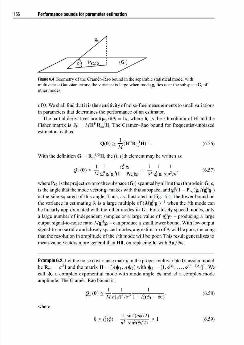
8/21/2019 Statistical Signal Processing of Complex-Valued Data.pdf
http://slidepdf.com/reader/full/statistical-signal-processing-of-complex-valued-datapdf 188/330
166 Performance bounds for parameter estimation
gi
PGigi ri Gi
Figure 6.4 Geometry of the Cramer–Rao bound in the separable statistical model with
multivariate Gaussian errors; the variance is large when mode gi lies near the subspace Gi of
other modes.
of . We shall find that it is the sensitivity of noise-free measurements to small variations
in parameters that determines the performance of an estimator.
The partial derivatives are ∂ y /∂θ i = hi , where hi is the i th column of H and theFisher matrix is JF = M HHR −1nn H. The Cramer–Rao bound for frequentist-unbiased
estimators is thus
Q() ≥ 1
M (HHR −1
nn H)−1. (6.56)
With the definition G = R −1/2nn H, the (i, i )th element may be written as
Qii () ≥ 1
M
1
gHi gi
gHi gi
gHi (I − PGi
)gi
= 1
M
1
gHi gi
1
sin2ρi
, (6.57)
where PGi is the projection onto thesubspace Gi spanned by all but the i thmodein G, ρi
is the angle that the mode vector gi makes with this subspace, and gHi (I − PGi
)gi /(gHi gi )
is the sine-squared of this angle. Thus, as illustrated in Fig. 6.4, the lower bound on
the variance in estimating θ i is a large multiple of ( M gHi gi )
−1 when the i th mode can
be linearly approximated with the other modes in Gi . For closely spaced modes, only
a large number of independent samples or a large value of gHi gi – producing a large
output signal-to-noise ratio M gHi gi – can produce a small lower bound. With low output
signal-to-noise ratio and closely spaced modes, any estimator of θ i will be poor, meaning
that the resolution in amplitude of the i th mode will be poor. This result generalizes to
mean-value vectors more general than H, on replacing hi with ∂ /∂θ i .
Example 6.2. Let the noise covariance matrix in the proper multivariate Gaussian model
be R nn = σ 2I and the matrix H = [ A1, A2] with k = [1, e jφk , . . . , e j(n−1)φk ]T. We
call k a complex exponential mode with mode angle φk and A a complex mode
amplitude. The Cramer–Rao bound is
Qii () ≥ 1
M
1
n
| A
|2/σ 2
1
1
−l 2n (φ1
−φ2)
, (6.58)
where
0 ≤ l 2n(φ) = 1
n2
sin2(nφ/2)
sin2(φ/2) ≤ 1 (6.59)
8/21/2019 Statistical Signal Processing of Complex-Valued Data.pdf
http://slidepdf.com/reader/full/statistical-signal-processing-of-complex-valued-datapdf 189/330
6.3 Fisher score and the Cram´ er–Rao bound 167
is the Lanczos kernel. In this bound, snr = | A|2/σ 2 is the per-sample or input signal-
to-noise ratio, SNR = nsnr is the output signal-to-noise ratio and 1 − l 2n(φ1 − φ2) is
the sine-squared of the angle between the subspaces 1 and 2. This bound is
( M SNR)−1
at φ1 − φ2 = 2π/ n, and this angle difference is called the Rayleigh limit to resolution. It governs much of optics, radar, sonar, and geophysics, even though it is
quite conservative in the sense that many independent samples or large input SNR can
override the aperture effects of the Lanczos kernel.2
This example bounds the error covariance matrix for estimating the linear param-
eters in the separable linear model, not the nonlinear parameters that would deter-
mine the matrix H(). Typically these parameters would be frequency, wavenumber,
delay, and so on. The Cramer–Rao bound for these parameters then depends on terms
like ∂ hi /∂θ ∗ j .3
6.3.4 Extension of Fisher score and the Cram´ er–Rao bound to improper
errors and scores
In order to extend the Cramer–Rao bound to improper errors and scores, we need only
compute the complementary expansion-coefficient matrix T() = E [s(y)eT(y)] and
complementary Fisher information matrix J() = E [s(y)sT(y)]. To this end, consider
the following conjugate partial derivative of the bias:
∂
∂∗ b() = ∂
∂∗ [(y) − ] p(y)d y
=
[(y) − ]
∂
∂∗ log p(y)
p(y)d y − 0 = TT(). (6.60)
This produces the identity
T() =
∂
∂b∗()
H
=
∂
∂∗ b()
T
. (6.61)
The (i,
j )th element of the matrix (∂/∂
∗)b
(
) is (∂/∂θ
∗ j )bi (
). Importantly, for fre-quentist unbiased estimators, the complementary expansion-coefficient matrix is zero,
and the augmented expansion-coefficient matrix is T() = I.
For the complementary Fisher information, consider the p × p Hessian
∂
∂
∂
∂log p(y)
T
= ∂
∂
∂
∂ p(y)
T1
p(y)
= ∂
∂
∂
∂ p(y)
T1
p(y) −
∂
∂log p(y)
T∂
∂log p(y). (6.62)
Taking expectations, we find the identity
JF() = E [s(y)sT (y)] = − E
∂
∂
∂
∂log p(y)
T
, (6.63)
8/21/2019 Statistical Signal Processing of Complex-Valued Data.pdf
http://slidepdf.com/reader/full/statistical-signal-processing-of-complex-valued-datapdf 190/330
168 Performance bounds for parameter estimation
which is the complementary dual to (6.45). The augmented Cramer–Rao bound for
improper error and measurement scores is the bound of Result 6.3, applied to the Fisher
score.
Result 6.5. For frequentist-unbiased estimators, the widely linear Cram´ er–Rao bound is
Q() ≥ [JF() − JF()J−∗F ()J∗F()]−1. (6.64)
Since [JF() − JF()J−∗F ()J∗F()]−1 ≥ J−1F (), the widely linear bound is tighter than
the standard Cramer–Rao bound in Result 6.4, which ignores complementary Fisher
information. Result 6.5 was essentially given by van den Bos (1994b).
Note that Results 6.3 and 6.5 assume that JF() is nonsingular. An important
case in which JF() is always singular is when the parameter is real . For real
, we have JF() = JF(), so there is no need to compute the complementaryFisher matrix. In this case, widely linear estimation of the error from the measure-
ment score is equivalent to linear estimation, and the widely linear Cramer–Rao
bound is the standard Cramer–Rao bound: Q() ≥ J−1F (). However, this bound still
depends on whether or not y is proper because even the Hermitian Fisher matrix
JF() depends on the complementary correlation of y, as the following subsection
illustrates.
6.3.5 The Cram ´ er–Rao bound in the improper multivariate Gaussian model
It is straightforward to extend the results of Section 6.3.2 to improper Gaussians. Let
y: −→ Cn be Gaussian with augmented mean y and augmented covariance matrix
R yy . Assuming as before that we have drawn M independent copies of y, the (i, j )th
element of the Hermitian Fisher matrix is
J F,i j = M
2 tr
R −1
yy
∂
∂θ iR yy
R −1
yy
∂
∂θ ∗ j
R yy
+ M
∂
∂θ i
y
H
R −1 yy
∂
∂θ ∗ j
y
= J ∗F, ji ,
(6.65)
where the second summand is real. The (i, j )th element of the complementary Fisher matrix is
˜ J F,i j = M
2 tr
R −1
yy
∂
∂θ iR yy
R −1
yy
∂
∂θ j
R yy
+ M
∂
∂θ i
y
HR −1
yy
∂
∂θ j
y
= ˜ J F, ji ,
(6.66)
and again the secondsummand is real. The caseof real , JF() = JF(), has been treated
by Delmas and Abeida (2004). They have shown that, when is real, the Cramer–Rao
bound Q() ≥ J−1F () is actually lowered if y is improper rather than proper. That is,
for a given Hermitian covariance matrix R yy , the Hermitian Fisher matrix JF() is more positive definite if R yy = 0 than if R yy = 0. At first, this may seem like a contradiction
of the statement made after Result 6.5 that improper errors and scores tighten (i.e.,
increase) the Cramer–Rao bound. So what is going on?

8/21/2019 Statistical Signal Processing of Complex-Valued Data.pdf
http://slidepdf.com/reader/full/statistical-signal-processing-of-complex-valued-datapdf 191/330
6.3 Fisher score and the Cram´ er–Rao bound 169
There are two different effects at work. On the one hand, the actual mean-squared
error in widely linearly estimating (real or complex) from y is reduced when the
degree of impropriety of y is increased while the Hermitian covariance matrix R yy is
kept constant. This is reflected by the lowered Cram´er–Rao bound. On the other hand,
if is complex, a widely linear estimate of the error score from the measurement score
is a more accurate predictor of the actual mean-squared error for estimating from y
than is a linear estimate of the error score from the measurement score. This is reflected
by a tightening Cramer–Rao bound. It depends on the problem which one of these two
effects is stronger.
Finally, we note that (6.65) and(6.66) do not cover the maximally improper (also called
strictly noncircular or rectilinear ) case in which R yy is singular. This was addressed by
R omer and Haardt (2007).
6.3.6 Fisher score and Cram ´ er–Rao bounds for functions of parameters
Sometimes it is a function of the parameter that is to be estimated rather than the
parameter itself. What can we say about the Fisher matrix in this case? Let w = g()
be a continuous bijection from C p to C p, with inverse = g−1(w). In the linear case,
w = H and = H−1w, and in the widely linear case, w = H and = H−1w. Define
the Jacobian matrix
F(w) = ∂∂w
= F(w) F(w)F∗(w) F∗(w) =
∂
∂w
∂
∂w∗ ∂
∂w∗
∗ ∂
∂w
∗. (6.67)
In the linear case, F(w) = H−1 and F = 0. In the widely linear case, F(w) = H−1. The
pdf parameterized by w is taken to be p(y) at = g−1(w). Using the chain rule for
non-holomorphic functions (A2.23), the Fisher score for w is then
sw(y) = ∂
∂wlog pw(y)
H
= ∂
∂log p(y)F(w) + ∂
∂∗
log p(y)F∗(w)
H
= FH(w)s(y) + FT(w)s∗(y) at = g(w),
or, equivalently,
sw(y) = FH(w)s(y) at = g(w), (6.68)
where s(y) is the augmented Fisher score for . If g is widely linear, then sw(y) =H−Hs(y).
The centered error in estimating w is ew(y)
=g−1(e(y)). In the widely linear case, we
have ew(y) = H e(y). The expansion-coefficient matrix cannot be modeled generally, but for widely linear g the augmented version is
T(w) = E [sw(y)eHw(y)] = H−HT()HH at = H−1w. (6.69)
8/21/2019 Statistical Signal Processing of Complex-Valued Data.pdf
http://slidepdf.com/reader/full/statistical-signal-processing-of-complex-valued-datapdf 192/330
170 Performance bounds for parameter estimation
The augmented Fisher matrix for w is
JF(w) = FH(w)JF()F(w) at = g−1(w). (6.70)
If g is widely linear, this is JF(w) = H−H
JF()H−1
at = H−1
w. So, in the general casewe can characterize the Fisher matrix and in the widely linear case we can characterize
the Cramer–Rao bound:
Q(w) ≥ TH(w)J−1F (w)T(w) = H TH()J−1
F ()T()HH at = H−1w. (6.71)
If the original estimator was frequentist unbiased, then T() = I and the bound is
Q(w) ≥ H J−1F ()HH at = H−1w. (6.72)
To obtain a bound on Q(w), we read out the northwest block of Q(w). The simplifications
in the strictly linear case should be obvious.
6.4 Quadratic Bayesian bounds
As in the development of quadratic frequentist bounds, the idea of quadratic Bayesian
bounds is this: from the measurement y is computed the estimator (y), with error
(y, ) = (y) − and centered error score e(y, ) = (y, ) − b. We would like to
approximate this centered error score by using a linear or widely linear function of
the centered measurement score s(y, ) = (y, ) − E [(y, )]. Thus, the virtual two-channel estimation problem of Fig. 6.2 still holds. The centered error score e(y, ) is to
be estimated from the centered measurement score s(y, ).
We will from the outset discuss the widely linear story, and the simplifications in the
linear case should be obvious. The composite vector of augmented centered errors and
scores [eT, sT]T has covariance matrix
E
e(y, )
s(y, )
eH(y, ) sH(y, )
=
Q TH
T J
. (6.73)
In this equation the covariance matrices Q, T, and J are defined as
Q = E [e(y, )eH(y, )],
T = E [s(y, )eH(y, )], (6.74)
J = E [s(y, )sH(y, )],
where Q is the augmented error covariance for the estimator (y), T is the augmented
sensitivity or expansion-coefficient matrix, and J is the augmented information matrix
associated with the centered measurement score s(y, ). In the case of the Fisher–Bayes
score, to be discussed in Section 6.5, the information is Fisher–Bayes information.The covariance matrix for the composite augmented error and score is positive
semidefinite, so, assuming the augmented information matrix to be nonsingular, we
obtain the following bound.
8/21/2019 Statistical Signal Processing of Complex-Valued Data.pdf
http://slidepdf.com/reader/full/statistical-signal-processing-of-complex-valued-datapdf 193/330
6.5 Fisher–Bayes score and Fisher–Bayes bound 171
Result 6.6. The augmented error covariance is bounded by the general augmented
quadratic Bayesian bound
Q≥
THJ−1T. (6.75)
The augmented mean-squared error matrix is bounded by
M ≥ THJ−1T + b bH. (6.76)
The bounds on Q and M are obtained by reading out the northwest block of Q and M.
Only the choice of score distinguishes one bound from another. Moreover, all quadratic
Bayes bounds are invariant with respect to nonsingular widely linear transformation
of the score function s. That is, the transformed score L s transforms the augmented
sensitivity matrix T to L T and the augmented information matrix J to L J LH
, leavingthe bound invariant.
Definition 6.4. A widely linear estimator will be said to be Bayes-efficient with respect
to a given score if the bound in ( 6.75 ) is achieved with equality.
A necessary and sufficient condition for efficiency is
(y) − − ( E [] − E []) = THJ−1s(y, ) (6.77)
which is also invariant with respect to widely linear transformation L. That is,an estimator is efficient if, element-by-element, the centered error scores lie in
the widely linear subspace spanned by the elements of the centered measurement
score.
The minimum achievable error covariance will be the covariance of the conditional
mean estimator, which is unbiased. Thus, the Fisher–Bayes bound will be the greatest
achievable quadratic lower bound if and only if the conditional mean estimator can be
written as E [|y] = THJ−1s(y, ) + . This result follows from the fact that the MMSE
estimator has zero mean, which is to say that E [ (y)] = E [].
The comments in Section 6.2.1, regarding good and bad scores, and Section 6.2.2apply almost directly to Bayesian bounds, with one cautionary note: the Bayes expansion
coefficient t i = E [ si (y, θ )e∗(y, θ )] is not generally E [t i (θ )] = E { E θ [t i (θ )]}, since the
frequentist’s score sθ (y) is not generally the Bayesian’s score s(y, θ ), which will include
prior information about the parameter θ .
6.5 Fisher–Bayes score and Fisher–Bayes bound
Our results for quadratic Bayes bounds so far are general. To make them applicable, weneed to consider a concrete score for which the augmented covariances T and J can be
computed. Following the development of the Fisher score, we choose the Fisher–Bayes
score and compute its associated Fisher–Bayes bound .
8/21/2019 Statistical Signal Processing of Complex-Valued Data.pdf
http://slidepdf.com/reader/full/statistical-signal-processing-of-complex-valued-datapdf 194/330
172 Performance bounds for parameter estimation
6.5.1 Fisher–Bayes score and information
Definition 6.5. The Fisher–Bayes measurement score is defined as
(y, ) = ∂∂
log p(y, )H
= ∂∂θ ∗1
log p(y, ), . . . , ∂∂θ ∗ p
log p(y, )T
. (6.78)
As throughout this chapter, all partial derivatives are Wirtinger derivatives as defined
in Appendix 2. Thus, the Fisher–Bayes score is a p-dimensional complex column vector.
The Fisher–Bayes score is the sum of the Fisher score and the prior score,
(y, ) =
∂
∂log p(y, )
H
= ∂
∂ log p(y)H
+ ∂
∂ log p()H
= (y) + (), (6.79)
where (y) is the frequentist score and () is a new score that scores the prior
density. The pdf p(y, ) is the joint pdf for the measurement y and parameter . Since
the expected value of Fisher–Bayes score is 0, Definition 6.5 also defines the centered
measurement score s(y, ).
There are several properties of the Fisher–Bayes score that make it a compelling
statistic for inferring the valueof a parameter and for bounding the mean-squared errorof
any estimator for that parameter. In the following list, properties 1, 2, and 4 are analogous
to the properties of the Fisher score listed in Section 6.3, but property 3 is different.
1. We may write the partial derivative as
∂
∂θ ∗ilog p(y, ) = 1
p(y, )
∂
∂θ ∗i p(y, ), (6.80)
which is a normalized measure of the sensitivity of the pdf p(y, ) to variations in the
parameter θ i . Large sensitivity is valued, and this will be measured by the variance
of the score.
2. The Fisher–Bayes score is a zero-mean random variable. This statistical property is
consistent with maximum-likelihood procedures that search for maxima of the log-
likelihood function log p(y, ) by searching for zeros of (∂/∂)log p(y, ). Functions
with steep slopes are valued, so we value a zero-mean score with large variance.
3. The expansion-coefficient matrix is T = I, and the complementary expansion-
coefficient matrix is T = 0, thus T = I. So, for the Fisher–Bayes measurement score,
the centered measurement score is perfectly aligned with the centered error score.
4. The Fisher–Bayes information matrix is also the expected Hessian of the score
function (up to a minus sign):
JFB
= E s(y, )sH(y, ) = E
∂
∂
log p(y, )H
∂
∂
log p(y, )= − E
∂
∂
∂
∂log p(y, )
H
. (6.81)
8/21/2019 Statistical Signal Processing of Complex-Valued Data.pdf
http://slidepdf.com/reader/full/statistical-signal-processing-of-complex-valued-datapdf 195/330
6.5 Fisher–Bayes score and Fisher–Bayes bound 173
Analogously, the complementary Fisher–Bayes information matrix is
JFB = E [s(y, )sT(y, )] = − E
∂
∂ ∂
∂log p(y, )
T
. (6.82)
The proofs of properties 2 and 4 for the Fisher–Bayes score are not substantially
different than the corresponding proofs for the Fisher score, so we omit them. Property
3 is proved as follows. The bias b of the parameter estimator is differentiated with
respect to as
0 =
∂
∂b
H
=
∂
∂
((y) − ) p(y, )d y d
H
= ∂
∂log p(y, )
H
[(y)−
]H p(y, )d y d −
I=
T−
I, (6.83)
which produces the identity T = I. On the other hand, the complementary expansion-
coefficient matrix is derived analogously by considering
0 =
∂
∂b∗H
=
∂
∂
((y) − )∗ p(y, )d y d
H
=
∂
∂log p(y)
H
[(y) − ]T p(y, )d y d − 0 =
T. (6.84)
This shows that T = 0, which means that the error and Fisher–Bayes score are alwayscross-proper. This is a consequence of the way the Fisher–Bayes score is defined. In
summary, the augmented expansion-coefficient matrix is T = I.
The Fisher–Bayesmatrix JFB is the sum of the expected Fisher matrix and the expected
prior information matrix, since the frequentist score and prior score are uncorrelated:
JFB = E [JF()] + E [JP()]. (6.85)
Thus, the Fisher–Bayes information is not simply the average of the Fisher information,
although, for diffuse priors or a plenitude of measurements, it is approximately so.
6.5.2 Fisher–Bayes bound
The Fisher–Bayes bound on the augmented error covariance matrix is Result 6.6 with
Fisher–Bayes score: Q ≥ J−1FB . From it, we obtain the bound on the error covariance
matrix.
Result 6.7. The widely linear Fisher–Bayes bound on the error covariance matrix is
Q
≥(JFB
− JFBJ−∗FB J∗FB)−1. (6.86)
The Fisher–Bayes bound is sometimes also called the stochastic Cram´ er–Rao bound .
In a number of aspects it behaves essentially like the “deterministic” Cramer–Rao bound
in Result 6.4.
8/21/2019 Statistical Signal Processing of Complex-Valued Data.pdf
http://slidepdf.com/reader/full/statistical-signal-processing-of-complex-valued-datapdf 196/330
174 Performance bounds for parameter estimation
The widely linear Fisher–Bayes bound is tighter than the linear Fisher–Bayes bound
ignoring complementary Fisher–Bayes information because (JFB − JFBJ−∗FB J∗FB)−1 ≥J−1
FB . However, JFB itself depends on whether or not y is proper. If M repeated measurements carry information about one fixed parameter through
the product pdf M i=1 p(yi , ), the Fisher–Bayes bound decreases as M −1.
The influence of nuisance parameters on the Fisher–Bayes bound remains unchanged
from Section 6.3.1: nuisance parameters increase the Fisher–Bayes bound. A tractable formula forFisher–Bayes bounds forfunctions ofparameters isobtained for
the widely linear case, in which the development of Section 6.3.6 proceeds essentially
unchanged.
Suppose that measurement and parameter have a jointly Gaussian distribution
p(y, ) = p(y) p(), and has augmented covariance matrix R θ θ . The new term added
to the Fisher information matrix to produce the Fisher–Bayes information matrix is the prior information JP = R −1
θ θ , which is independent of the mean of . Consequently the
augmented Fisher–Bayes bound is
Q ≥ (JF + R −1θθ )
−1, (6.87)
where JF = E [JF()] and the elements of the augmented Fisher matrix JF() have been
derived in Section 6.3.5.
6.6 Connections and orderings among bounds
Generally, we would like to connect Bayesian bounds to frequentist bounds, and partic-
ularly the Fisher–Bayes bound to the Cramer–Rao bound. In order to do so, we appeal
to the fundamental identity
Q = E [Q()] + R bb . (6.88)
Thus, there is the Bayesian bound
Q ≥ E [TH
()J−1
()T()] + E [(b() − b)(b() − b)H
]. (6.89)
This is a covariance bound on any estimator whose frequentist bias is b() and Bayes
bias is b. If the frequentist bias is constant at b – as for LMVDR (BLUE) estimators,
for which b() = 0 – then R bb = 0, and the bound is Q ≥ E [TH()J−1()T()]. If the
score is the Fisher score, and the bias is constant, then T() = I and the bound is
Q ≥ E [J−1F ()]. (6.90)
This is a bound on any estimator of a random parameter with the property that its
frequentist and Bayes bias are constant, as in LMVDR estimators. We know this bound
is larger than the Fisher–Bayes bound, because JFB = E [JF()] + E [JP()], so we have
the ordering
E [J−1F ()] ≥ J−1
FB . (6.91)
8/21/2019 Statistical Signal Processing of Complex-Valued Data.pdf
http://slidepdf.com/reader/full/statistical-signal-processing-of-complex-valued-datapdf 197/330
Notes 175
Thisordering makes sense because the right-hand side is a bound on estimators for which
there is no constraint on the frequentist bias, as in MMSE estimation, and the left-hand
side is a bound on estimators for which there is the constraint that the frequentist bias
be constant. The constraint increases error covariance, as we have seen when comparing
the variance of LMVDR and MMSE estimators.
When there is a plenitude of data or when the prior is so diffuse that E [JP()] E [JF()], then E [JF()] approximates JFB from below andconsequently ( E [JF()])−1 ≥J−1
FB . Then, by Jensen’s inequality, E [J−1F ()] ≥ ( E [JF()])−1, so we may squeeze
( E [JF()])−1 between the two bounds to obtain the ordering (cf. Van Trees and Bell
(2007))
E [J−1F ()] ≥ ( E [JF()])−1 ≥ J−1
FB . (6.92)
To reiterate, the rightmost inequality follows from the fact that the Fisher–Bayesinformation matrix is more positive semidefinite than the expected value of the Fisher
information matrix. The leftmost follows from Jensen’s inequality.
Why should this ordering hold? The leftmost bound is a bound for estimators that are
frequentist and Bayes unbiased, and frequentist unbiasedness is not generally a desir-
able property for an estimator of a random parameter. So this extra property tends to
increase mean-squared error. The middle term ignores prior information about the ran-
dom parameter, so it is only a bound in the limit as the Fisher–Bayes information matrix
converges to the expected Fisher information matrix. The rightmost bound enforces
no constraints on the frequentist or Bayes bias. The leftmost bound we tend to asso-ciate with LMVDR and ML estimators, the middle term we associate with the limiting
performance of MMSE estimators when the prior is diffuse or there is a plenitude of
measurements, and the rightmost bound we tend to associate with MMSE estimators.
In fact, in our examples we have seen that the LMVDR and ML estimators achieve
the leftmost bound and the MMSE estimator achieves the rightmost. Of course, it is
not possible or meaningful to fit the frequentist Cramer–Rao bound into this ordering,
except when JF() is independent of , in which case J−1F = E [J−1
F ] = ( E [JF])−1. Then
J−1F ≥ J−1
FB .
Notes
1 There is a vast literature on frequentist and Bayesian bounds. This literature is comprehensively
represented, with original results by the editors, in Van Trees and Bell (2007). We make no
attempt in this chapter to cite a representative subset of theoretical and applied papers in this
edited volume, or in the published literature at large, since to do so would risk offense to the
authors of the papers excluded.
This chapter addresses performance bounds for the entire class of quadratic frequentist and
Bayesian bounds, for proper and improper complex parameters and measurements. Our method
has been to cast the problem of quadratic performance bounding in the framework of error score
estimation from measurement scores in a virtual two-channel experiment. This point of view is
consistent with the point of view used in Chapter 5 and it allows us to extend the reasoning of
Weinstein and Weiss (1988) to widely linear estimators.
8/21/2019 Statistical Signal Processing of Complex-Valued Data.pdf
http://slidepdf.com/reader/full/statistical-signal-processing-of-complex-valued-datapdf 198/330
176 Performance bounds for parameter estimation
We have not covered the derivation of performance bounds under parameter constr aints.
Representative published works are those by Gorman and Hero (1990), Marzetta (1993), and
Stoica and Ng (1998).
2 The examples we give in this chapter are not representative of a great number of problems in
signal processing where mode parameters like frequency, wavenumber, direction of arrival, and so on are to be estimated. In these problems the Cramer–Rao and Fisher–Bayes bounds are
tight at high SNR and very loose at low SNR. Consequently they do not predict performance
breakdown at a threshold SNR. In an effort to analyze the onset of breakdown, many alternative
scores have been proposed. Even the Cramer–Rao and Fisher–Bayes bounds can be adapted
to this problem by using a method of intervals, wherein a mixture of the Cramer–Rao or
Fisher–Bayes bound and a constant bound representative of total breakdown is averaged. The
averaging probability is the probability of error lying outside the interval wherein the likelihood
is quadratic, and it may be computed for many problems. This method, which has been used to
effect by Richmond (2006), is remarkably accurate. So we might say that quadratic performance
bounding, augmented with a method of intervals, is a powerful way to model error covariances
from high SNR, through the threshold region of low SNR where the quadratic bound by itself is not tight, to the region of total breakdown.
3 The Cramer–Rao bounds for these nonlinear parameters have been treated extensively in the
literature, and are well represented by Van Trees and Bell (2007). McWhorter and Scharf
(1993b) discuss concentration ellipsoids for error covariances when estimating the sum and
difference frequencies of closely spaced modes within the matrix H(). See also the discussion
of the geometry of the Cramer–Rao bound by McWhorter and Scharf (1993a).
8/21/2019 Statistical Signal Processing of Complex-Valued Data.pdf
http://slidepdf.com/reader/full/statistical-signal-processing-of-complex-valued-datapdf 199/330
7 Detection
Detection is the electrical engineer’s term for the statistician’s hypothesis testing . The
problem is to determine which of two or more competing models best describes exper-
imental measurements. If the competition is between two models, then the detection
problem is a binary detection problem. Such problems apply widely to communication,
radar, and sonar. But even a binary problem can be composite, which is to say that one
or both of the hypotheses may consist of a set of models. We shall denote by H 0 the
hypothesis that the underlying model, or set of models, is M 0 and by H 1 the hypothesis
that it is M 1.
There are two main lines of development for detection theory: Neyman–Pearson
and Bayes. The Neyman–Pearson theory is a frequentist theory that assigns no prior
probability of occurrence to the competing models. Bayesian theory does. Moreover, the
measure of optimality is different. To a frequentist the game is to maximize the detection
probability under the constraint that the false-alarm probability is not greater than a pre-
specified value. To a Bayesian the game is to assign costs to incorrect decisions, and
then to minimize the average (or Bayes) cost. The solution in any case is to evaluate the
likelihood of the measurement under each hypothesis, and to choose the model whose
likelihood is higher. Well – not quite. It is the likelihood ratio that is evaluated, and when
this ratio exceeds a threshold, determined either by the false-alarm rate or by the Bayes
cost, one or other of the hypotheses is accepted.
It is commonplace for each of the competing models to contain unknown nuisance
parameters and unknown decision parameters. Only the decision parameters are tested,
but the nuisance parameters complicate the computation of likelihoods and defeatattempts at optimality. There are generally two strategies: enforce a condition of invari-
ance, which limits competition to detectors that share these invariances, or invoke a
principle of likelihood that replaces nuisance parameters by their maximum-likelihood
estimates. These lead to generalized likelihood ratios. In many cases the two approaches
produce identical tests. So, in summary, the likelihood-ratio statistic is the gold standard.
It plays the same role for binary hypothesis testing as the conditional mean estimator
plays in MMSE estimation.
The theory of Neyman–Pearson and Bayes detection we shall review is quite gen-
eral.1 It reveals functions of the measurement that may include arbitrary functions of the complex measurement y, including its complex conjugate y∗. However, in order
to demonstrate the role of widely linear and widely quadratic forms in the theory of
8/21/2019 Statistical Signal Processing of Complex-Valued Data.pdf
http://slidepdf.com/reader/full/statistical-signal-processing-of-complex-valued-datapdf 200/330
178 Detection
hypothesis testing, we shall concentrate on hypothesis testing within the proper and
improper Gaussian measurement models.
Throughout this chapter we assume that measurements have pdfs, which are allowed
to contain Dirac δ-functions. Thus, all of our results hold for mixed random variables
with discrete and continuous, and even singular, components.
7.1 Binary hypothesis testing
A hypothesis is a statement about the distribution of a measurement y ∈ Y . Typi-
cally the hypothesis is coded by a parameter ∈Θ that indexes the pdf p(y) for
the measurement random vector y: −→ Cn . We might say the parameter modu-
lates the measurement in the sense that the value of modulates the distribution
of the measurement. Often the parameter modulates the mean vector, as in com-
munications, but sometimes it modulates the covariance matrix, as in oceanogra-
phy and optics, where a frequency–wavenumber spectrum determines a covariance
matrix.
We shall be interested in two competing hypotheses, H 0 and H 1, and therefore we
address ourselves to binary hypothesis testing , as opposed to multiple hypothesis testing .
The hypothesis H 0 is sometimescalledthehypothesisand thehypothesis H 1 is sometimes
called the alternative, so we are testing a hypothesis against its alternative. Each of the
hypotheses may be simple, in which case the pdf of the measurement is pi(y) under
hypothesis H i . Or each of them may be composite, in which case the distribution of
the measurement is p(y), ∈Θi , under hypothesis H i . The parameter setsΘi and the
measurement space y ∈ Y may be quite general.
Definition 7.1. A binary test of H 1 versus H 0 is a test statistic , or threshold detector
φ: Y → {0, 1} of the form
φ(y) =
1, y ∈ Y 1,
0, y ∈ Y 0.(7.1)
We mightsay that φ is a one-bit quantizer of the random vector y. It sorts measurementsinto two sets: thedetection regionY 1 and itscomplement regionY 0. Such a test willmake
two types of errors: missed detections and false alarms. That is, it will sometimes classify
a measurement drawn from the pdf p(y), ∈Θ1, as a measurement drawn from the
pdf p(y), ∈Θ0. This is a missed detection. Or it might classify a measurement drawn
from the pdf p(y), ∈Θ0, as a measurement drawn from the pdf p(y), ∈Θ1. This
is a false alarm.
For a simple hypothesis and simple alternative the detection probability P D and the
false-alarm probability P F of a test are defined as follows:
P D = P 1(φ = 1) = E 1
[φ], (7.2)
P F = P 0(φ = 1) = E 0
[φ]. (7.3)
8/21/2019 Statistical Signal Processing of Complex-Valued Data.pdf
http://slidepdf.com/reader/full/statistical-signal-processing-of-complex-valued-datapdf 201/330
7.1 Binary hypothesis testing 179
The subscripts on the probability and expectation operators denote probability and
expectation computed under the pdf of the measurement pi(y). We shall generalize
these definitions for testing composite hypotheses in due course.
Detection probability and false-alarm probability are engineering terms for the statis-
tician’s power and size. Both terms are evocative, with the statistician advocating for a
test that is small but powerful, like a compact drill motor, and the engineer advocating
for a test that has high detection probability and low false-alarm probability, like a good
radar detector on one of the authors’ Mazda RX-7.
7.1.1 The Neyman–Pearson lemma
In binary hypothesis testing of a simple alternative versus a simple hypothesis, the test
statistic φ is a Bernoulli random variable B [ p], with p =
P D under H 1 and p =
P F under
H 0. Ideally, it would have the property P D = 1 and P F = 0, but these are unattainable
for non-degenerate tests. So we aim to maximize the detection probability under the
constraint that the false-alarm probability be no greater than the design value of P F = α.
In other words, it should have maximum power for its small size. We first state the
Neyman–Pearson (NP) lemma without proof.2
Result 7.1. (Neyman–Pearson) Among all competing binary tests φ of a simple alter-
native versus a simple hypothesis, with probability of false alarm less than or equal to
α , none has larger detection probability than the likelihood-ratio test
φ(y) =
1, l (y) > η,
γ , l (y) = η,
0, l (y) < η.
(7.4)
In this equation, 0 ≤ l (y) < ∞ is the real-valued likelihood ratio
l (y) = p1(y)
p0(y)
(7.5)
and the threshold parameters (η, γ ) are chosen to satisfy the following constraint on the
false-alarm probability:
P 0[l (y) > η] + γ P 0
[l (y) = η] = α. (7.6)
When φ(y) = γ , we select H 1 with probability γ , and H 0 with probability 1 − γ .
The likelihood ratio l is a highly compressed function of the measurement, return-
ing a nonnegative number, and the test function φ returns what might be called
a one-bit quantized version of the likelihood ratio. Any monotonic function of
the likelihood ratio l will do, so in multivariate Gaussian theory it is the loga-
rithm of l , or the log-likelihood ratio L, that is used in place of the likelihood-
ratio.There is a cautionary note about the reading of these equations. The test statistic φ
and the likelihood ratio l are functions of the measurement random variable, making φ
8/21/2019 Statistical Signal Processing of Complex-Valued Data.pdf
http://slidepdf.com/reader/full/statistical-signal-processing-of-complex-valued-datapdf 202/330
180 Detection
and l random variables. When evaluated at a particular realization or measurement, they
are test values and likelihood-ratio values.
7.1.2 Bayes detectorsTheonly thing that distinguishes a Bayes detector from a Neyman–Pearson(NP) detector
is the choice of threshold η. It is chosen to minimize the Bayes risk, which is defined
to be π1C 10(1 − P D) + (1 − π1)C 01 P F, where π1 is the prior probability that hypothesis
H 1 will be in force, C 10 is the cost of choosing H 0 when H 1 is in force, and 1 − P D is the
probability of doing so. Similarly, C 01 is the cost of choosing H 1 when H 0 is in force,
and P F is the probability of doing so.
Assume that the Bayes test sorts measurements into the set S ⊂ Cn , where H 1 is
accepted, and the complement set, where H 0 is accepted. Then the Bayes risk may be
written as
π1C 10(1 − P D) + (1 − π1)C 01 P F = π1C 10 +
S
[(1 − π1)C 01 p0(y) − π1C 10 p1
(y)]d y.
(7.7)
As in Chapter 6, this integral with respect to a complex variable is interpreted as the
integral with respect to its real and imaginary parts: f (y)d y
f (y)d[Re y]d[Im y]. (7.8)
The Bayes risk is minimized by choosing S in (7.7) to be the set
S = {y: π1C 10 p1(y) > (1 − π1)C 01 p0
(y)} =
y: l (y) >(1 − π1)C 01
π1C 10
= η
. (7.9)
This is just the likelihood-ratio test with a particular threshold η. The only difference
between a Bayes test and an NP test is that their thresholds are different.
7.1.3 Adaptive Neyman–Pearson and empirical Bayes detectors
It is often the case that only a subset of the parameters is to be tested, leaving the others
as nuisance parameters. In these cases the principles of NP or Bayes detection may be
expanded to say that unknown nuisance parameters are replaced by their maximum-
likelihood estimators or their Bayes estimators, under each of the two hypotheses.
The resulting detectors are called adaptive, empirical , or generalized likelihood-ratio
detectors. The literature on them is comprehensive, and we make no attempt to review it
here. Some examples are discussed in the context of testing for correlation structure in
Section4.5. Later, in Section 7.6, we outlinea different story, whichisbasedon invariance
with respect to nuisance parameters. This story also leads to detectors that are adaptive.
7.2 Sufficiency and invariance
The test function φ is a Bernoulli random variable. Its probability distribution depends
on the parameter according to p = P D under H 1 and p = P F under H 0. However,

8/21/2019 Statistical Signal Processing of Complex-Valued Data.pdf
http://slidepdf.com/reader/full/statistical-signal-processing-of-complex-valued-datapdf 203/330
7.3 Receiver operating characteristic 181
the value of φ, given its likelihood ratio l , is 0 if l < η, γ if l = η, and 1 if l > η,
independently of . Thus, according to the Fisher–Neyman factorization theorem, the
likelihood-ratio statistic is a sufficient statistic for testing H 1 versus H 0.
Definition 7.2. We call a statistic t(y) sufficient if the pdf p(y) may be factored as p(y) = a(y)q(t) , where q(t) is the pdf for the sufficient statistic.
In this case the likelihood ratio equals the likelihood ratio for the sufficient statistic t:
l (y) = p1(y)
p0(y)
= q1(t)
q0(t) = l (t). (7.10)
We may thus rewrite the NP lemma in terms of the sufficient statistic:
φ(t) = 1, l (t) > η,
γ , l (t) = η,
0, l (t) < η.
(7.11)
In this equation, (η, γ ) are chosen to satisfy the false-alarm probability constraint:
P 0[l (t) > η] + γ P 0
[l (t) = η] = α. (7.12)
The statistic t is often a scalar function of the original measurement, and its likeli-
hood can often be inverted with a monotonic function for the statistic itself. Then the
test statistic is a threshold test that simply compares the sufficient statistic against a
threshold.
Definition 7.3. A sufficient statistic isminimal , meaning that it is most memory efficient,
if it is a function of every other sufficient statistic. A sufficient statistic is an invariant
statistic with respect to the transformation group G if φ( g (t)) = φ(t) for all g ∈ G.
The composition rule for any two transformations within G is g 1 ◦ g 2(t) = g 1( g 2(t)).
7.3 Receiver operating characteristic
It is obvious that no NP detector will have a worse ( P D, P F) pair than (α, α), since the
test φ = α achieves this performance and, according to the NP lemma, cannot be better
than the NP likelihood-ratio test. Moreover, from the definitions of ( P D, P F), an increase
in the threshold η will decrease the false-alarm probability and decrease the detection
probability. So a plot of achievable ( P D, P F) pairs, called an ROC curve for receiver
operation characteristic, appears as the convex curve in Fig. 7.1.
Why is it convex? Consider two points on the ROC curve. Draw a straight line between
them, to find an operating point for some suboptimumdetector. At the P F for this detector
there is a point on the ROC curve for the NP detector that cannot lie below it. Thus theROC curve for the NP detector is convex.
Every detector will have an operating point somewhere within the convex set bounded
by the ROC curve for the NP detector and the (α, α) line. One such operating point is

8/21/2019 Statistical Signal Processing of Complex-Valued Data.pdf
http://slidepdf.com/reader/full/statistical-signal-processing-of-complex-valued-datapdf 204/330
182 Detection
10
1 slope h
P D
P F
Figure 7.1 Geometry of the ROC for a Neyman–Pearson detector.
illustrated with a cross in Fig. 7.1. Any suboptimum test with this operating point may
be improved with an NP test whose operating point lies on the arc subtended by the
wedge that lies to the northwest of the cross. To improve a test is to decrease its P F for a
fixed P D along the horizontal line of the wedge, increase its P D for a fixed P F along the
vertical line of the wedge, or decrease P F and increase P D by heading northwest to the
ROC line.
Recall the identity (7.10) for a sufficient statistic t. If the sufficient statistic is the
likelihood itself, that is t = l (y), (7.10) shows that the pdf for likelihood under the two
hypotheses is connected as follows:
q1(l ) = lq0
(l ). (7.13)
The probability of detection and probability of false alarm may be written
1 − P D = η
0
q1(l )d l =
η
0
lq0(l )d l , (7.14)
1−
P F =
η
0
q0
(l )d l . (7.15)
Differentiate each of these formulae with respect to η to find
∂
∂η P D = −ηq0
(η) (7.16)
∂
∂η P F = −q0
(η) (7.17)
and therefore
d P D
d P F= η. (7.18)
Thus, at any operating point on the ROC curve, the derivativeof the curve is the threshold
η required to operate there.3
8/21/2019 Statistical Signal Processing of Complex-Valued Data.pdf
http://slidepdf.com/reader/full/statistical-signal-processing-of-complex-valued-datapdf 205/330
7.4 Simple Gaussian hypothesis testing 183
7.4 Simple hypothesis testing in the improper Gaussian model
In the context of this book, where an augmented second-order theory that includes Her-
mitian and complementary covariances forms the basis for inference, the most importantexample is the problem of testing in the multivariate Gaussian model. We may test for
mean-value and/or covariance structure.
7.4.1 Uncommon means and common covariance
The first problem is to test the alternative H 1 that an improper Gaussian measure-
ment y has mean value 1 versus the hypothesis H 0 that it has mean value 0.
Under both hypotheses the measurement y has Hermitian correlation R = E 0[(y −
0)(y−
0)H]=
E 1
[(y−
1)(y−
1)H] and symmetric complementary covarianceR = E 0[(y − 0)(y − 0)T] = E 1
[(y − 1)(y − 1)T]. These covariances are coded
into the augmented covariance matrix
R =
R R R ∗ R ∗
. (7.19)
For convenience, we drop the subscripts on covariance matrices (R yy etc.) in this chapter.
Following Result 2.4, we may write down the pdf of the improper Gaussian vector y
under hypothesis H i :
pi(y) = 1
π n det1/2 R exp− 1
2(y −
i)HR −1(y −
i). (7.20)
Of course, this pdf also covers the proper case where R is block-diagonal. After some
algebra, the real-valued log-likelihood ratio may be expressed as the following widely
linear function of y:
L = log
p1
(y)
p0(y)
= − 1
2(y −
1)HR −1(y −
1) + 1
2(y −
0)HR −1(y −
0)
=(
1
−
0)HR −1(y
−y
0) (7.21)
with
y0 = 1
2
1+
0
. (7.22)
The log-likelihood ratio may be written as the inner product
L =
R −1(1−
0)H
(y − y0) = 2 Re {wH(y − y0)}, (7.23)
with
w = w
w∗ = R −1(1 − 0). (7.24)
Taking the inner product in (7.23) can be interpreted as coherent matched filtering . In
the proper case, the matching vector w simplifies to w = R −1(1 − 0).
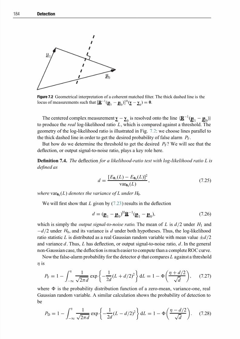
8/21/2019 Statistical Signal Processing of Complex-Valued Data.pdf
http://slidepdf.com/reader/full/statistical-signal-processing-of-complex-valued-datapdf 206/330
184 Detection
0µµ
µ1
Figure 7.2 Geometrical interpretation of a coherent matched filter. The thick dashed line is the
locus of measurements such that [R −1(1−
0)]H(y − y
0) = 0.
The centered complex measurement y − y0 is resolved onto the line R −1
(1 − 0)to produce the real log-likelihood ratio L , which is compared against a threshold. The
geometry of the log-likelihood ratio is illustrated in Fig. 7.2: we choose lines parallel to
the thick dashed line in order to get the desired probability of false alarm P F.
But how do we determine the threshold to get the desired P F? We will see that the
deflection, or output signal-to-noise ratio, plays a key role here.
Definition 7.4. The deflection for a likelihood-ratio test with log-likelihood ratio L is
defined as
d = [ E 1( L) − E 0( L)]2
var 0( L)
, (7.25)
where var 0( L) denotes the variance of L under H 0.
We will first show that L given by (7.23) results in the deflection
d = (1−
0)HR −1(
1−
0), (7.26)
which is simply the output signal-to-noise ratio. The mean of L is d /2 under H 1 and
−d /2 under H 0, and its variance is d under both hypotheses. Thus, the log-likelihood
ratio statistic L is distributed as a real Gaussian random variable with mean value ±d /2and variance d . Thus, L has deflection, or output signal-to-noise ratio, d . In the general
non-Gaussian case, the deflection is much easier to compute than a complete ROC curve.
Now the false-alarm probability for the detector φ that compares L against a threshold
η is
P F = 1 − η
−∞
1√ 2π d
exp
− 1
2d ( L + d /2)2
d L = 1 −
η + d /2√
d
, (7.27)
where is the probability distribution function of a zero-mean, variance-one, real
Gaussian random variable. A similar calculation shows the probability of detection to be
P D = 1 − η
−∞
1√ 2π d
exp
− 1
2d ( L − d /2)2
d L = 1 −
η − d /2√
d
. (7.28)

8/21/2019 Statistical Signal Processing of Complex-Valued Data.pdf
http://slidepdf.com/reader/full/statistical-signal-processing-of-complex-valued-datapdf 207/330
7.4 Simple Gaussian hypothesis testing 185
h + d 2√ d
h− d 2
d
d
P F
P D
L
Figure 7.3 The false-alarm probability P F (dark gray) and detection probability P D (light and
dark gray) are tail probabilities of a normalized Gaussian. They are determined by the threshold
η and the deflection d .
So, by choosing the threshold η, any design value of false-alarm probability may be
achieved, and this choice of threshold determines the detection probability as well. In
Fig. 7.3 the argument is made that the normalized zero-mean, variance-one, Gaussian
density determines performance. The designer is given a string of length√
d , whose
head end is placed at location (η + d /2)/√
d , to achieve the false-alarm probability P F,
and whose tail end falls at location (η − d /2)/√
d , to determine the detection probability
P D. The length of the string is√
d , which is the output voltage SNR, so obviously the
larger the SNR the better.
7.4.2 Common mean and uncommon covariances
When the mean of an improper complex randomvector is common to both the hypothesis
and the alternative, but the covariances are uncommon, we might as well assume that
the mean is zero, since the measurement can always be centered. Then the pdf for the
measurement y: −→ Cn under hypothesis H i is
pi(y)
=
1
πn
det
1/2
R i
exp−12
yHR −1i y (7.29)
where R i is the augmented covariance matrix under hypothesis H i . For a measured y
this is also the likelihood that the covariance model R i would have produced it. The
log-likelihood ratio for comparing the likelihood of alternative H 1 with the likelihood
of hypothesis H 0 is then the real widely quadratic form
L = yH(R −10 − R −1
1 )y = yHR −H/20 (I − S−1)R
−1/20 y, (7.30)
where S = R −1/20 R 1R
−H/20 is the augmented signal-to-noise ratio matrix. The trans-
formed measurement R −1/20 y has augmented covariance matrix I under hypothesis H 0
and augmented covariance matrix S under hypothesis H 1. Thus L is the log-likelihood ratio for testing that the widely linearly transformed measurement, extracted as the top
half of R −1/20 y, is proper and white versus the alternative that it is improper with aug-
mented covariance S. When the SNR matrix is given its augmented EVD S = UΛUH
8/21/2019 Statistical Signal Processing of Complex-Valued Data.pdf
http://slidepdf.com/reader/full/statistical-signal-processing-of-complex-valued-datapdf 208/330
186 Detection
(cf. Result 3.1), the log-likelihood-ratio statistic may be written
L = yHR −H/20 U(I −Λ−1)UHR
−1/20 y. (7.31)
The augmented EVD of the SNR matrix S is the solution to the generalized eigenvalue
problem
R 1(R −H/20 U) − R 0(R
−H/20 U)Λ = 0. (7.32)
The characteristic function for the quadratic form L may be derived, and inverted for its
pdf. We do not pursue this question further, since the general result does not bring much
insight into the performance of special cases.
7.4.3 Comparison between linear and widely linear detection
We would now like to compare the performance of linear and widely linear detection.
For this, we consider a special case of testing for a common mean and uncommon
covariances. We wish to detect whether the Gaussian signal x: −→ Cn is present in
additive white Gaussian noise n: −→ Cn . Under H 0, the measurement is y = n, and
under H 1, it is y = x + n. The signal x has augmented covariance matrix R x x and the
noise is white and proper with augmented covariance matrix R nn = N 0I. The signal and
noise both have zero mean, and they are uncorrelated. Thus, the covariance matrix under
H 0 is R 0 = N 0I, and under H 1 it is R 1 = R x x + N 0I.
Let R x x
=UΛUH denote the augmented EVD of R x x . Note that Λ is now the
augmented eigenvalue matrix of R x x , whereas before in Section 7.4.2, Λ denoted theaugmented eigenvalue matrix of S = R
−1/20 R 1R
−H/20 = R 1/ N 0 = R x x / N 0 + I. There-
fore, the augmented eigenvalue matrix of S is now Λ/ N 0 + I, and the log-likelihood
ratio (7.31) is
L = 1
N 0yHU[I − (Λ/ N 0 + I)−1]UHy
= 1
N 0yHUΛ(Λ+ N 0I)−1UHy. (7.33)
It is worthwhile to point out that L can also be written as L = yH(R x y R −1
yy y) = yHx = 2 Re {yHx}, (7.34)
where R x y = R x x and R yy = R 1 = R x x + N 0I, so that x is the widely linear MMSE
estimate of x from y. Hence, the log-likelihood detector for the signal-plus-white-noise
setup is really a cascade of a WLMMSE filter and a matched filter.
In the proper case, the augmented covariance matrix R x x is block-diagonal, R x x =Diag(R x x , R x x ), and the eigenvalues of R x x occur in pairs. Let M = Diag(µ1, . . . , µn)
be the eigenvalue matrix of the Hermitian covariance matrix R x x . The log-likelihood
ratio is now
L = 2
N 0Re {yHUM(M + N 0I)−1UHy} = 2 Re {yHx}, (7.35)
where x is now the linear MMSE estimate of x from y.
8/21/2019 Statistical Signal Processing of Complex-Valued Data.pdf
http://slidepdf.com/reader/full/statistical-signal-processing-of-complex-valued-datapdf 209/330
7.4 Simple Gaussian hypothesis testing 187
So what performance advantage does widely linear processing offer over linear pro-
cessing? Answering this question proceeds along the lines of Section 5.4.2. The perfor-
mance criterion we choose here is the deflection d . Schreier et al . (2005) computed the
deflection for the improper signal-plus-white-noise detection scenario:
d =
2ni=1
λ2i
λi + N 0
2
2 N 20
2ni=1
λi
λi + N 0
2. (7.36)
Here, {λi}2ni=1 are the eigenvalues of the augmented covariance matrix R x x . In order
to evaluate the maximum performance advantage of widely linear over linear pro-
cessing, we need to maximize the deflection for fixed R x x and varying R x x . UsingResult A3.3, it can be shown that the deflection is a Schur-convex function of the
eigenvalues {λi}. Therefore, maximizing the deflection requires maximum spread
of the {λi } in the sense of majorization. According to Result 3.7, this is achieved
for
λi = 2µi , i = 1, . . . , n, and λi = 0, i = n + 1, . . . , 2n, (7.37)
where {µi}ni=1 are the eigenvalues of the Hermitian covariance matrix R x x . By plug-
ging this into (7.36), we obtain the maximum deflection achieved by widely linear
processing,
maxR x x
d =2
ni=1
µ2i
2µi + N 0
2
N 20
ni=1
µi
2µi + N 0
2. (7.38)
On the other hand, linear processing implicitly assumes that
R x x = 0, in which case the
deflection is
d R x x=0 =
ni=1
µ2i
µi + N 0
2
N 20
ni=1
µi
µi + N 0
2. (7.39)
Thus, the maximum performance advantage, as measured by deflection, is
max N 0
max
R xx
d
d R xx =
0
= 2, (7.40)
which is attained for N 0 −→ 0 or N 0 −→∞. This bound was derived by Schreier et al .
(2005). We note that, if (7.37) is not satisfied, the maximum performance advantage,
which is then less than a factor of 2, occurs for some noise level N 0 > 0.
8/21/2019 Statistical Signal Processing of Complex-Valued Data.pdf
http://slidepdf.com/reader/full/statistical-signal-processing-of-complex-valued-datapdf 210/330
188 Detection
Thefactorof2 is a very conservativeperformance advantageboundbecause it assumes
the worst-case scenario of white additive noise. If the noise is colored, the performance
difference between widely linear and linear processing can be much larger. One such
example is the detection of a real message x in purely imaginary noise n. This is a trivial
detection problem, but only if the widely linear operation Re y is admitted.
7.5 Composite hypothesis testing and the Karlin–Rubin theorem
So far we have tested a simple alternative H 1 versus a simple hypothesis H 0 and found
the NP detector to be most powerful among all competitors whose false-alarm rates do
not exceed the false-alarm rate of the NP detector. Now we would like to generalize
the notion of most powerful to the notion of uniformly most powerful (UMP). That is,we would like to consider composite alternative and composite hypothesis and argue
that an NP test is uniformly most powerful, which is to say most powerful against all
competitors for every possible pair of parameters (0 ∈Θ0, 1 ∈ Θ1). This is too much
to ask, so we restrict ourselves to a scalar real-valued parameter θ , and ask for a test that
would be most powerful for every pair (θ 0 ∈ 0, θ 1 ∈ 1). Moreover, we shall restrict
the sets 0 and 1 to the form 0 = {θ : θ ≤ 0} and 1 = {θ : θ > 0}, or 0 = {0} and
1 = {θ : θ > 0}.
Definition 7.5. A detector φ is uniformly most powerful (UMP) for testing H 1: θ
∈1
versus H 0: θ ∈ 0 if its detection probability is greater at every value of θ ∈ 1 than
that of every competitor φ whose false-alarm probability is no greater than that of φ .
That is
supθ ∈0
E θ [φ] ≤ supθ ∈0
E θ [φ] = α, (7.41)
E θ [φ] ≤ E θ [φ], ∀ θ ∈ 1. (7.42)
A scalar sufficient statistic, such as the likelihood ratio itself, has been identified.
Assume that the likelihood ratio for this statistic, namely qθ 1(t )/qθ 0(t ) is monotonicallyincreasing in t for all θ 1 > θ 0. Then the test function φ may be replaced by the threshold
test
φ(t ) =
1, t > t 0,
γ , t = t 0,
0, t < t 0
(7.43)
with (t 0, γ ) chosen to satisfy the false-alarm probability. That is
P θ 0[t > t 0] + γ P θ 0[t = t 0] = α. (7.44)
The Karlin–Rubin theorem, which we shall not prove, says the threshold test φ is
uniformly most powerful for testing {θ ≤ 0} versus {θ > 0} or for testing {θ = 0} versus
{θ > 0}. Moreover, the false-alarm probability is computed at θ = 0.
8/21/2019 Statistical Signal Processing of Complex-Valued Data.pdf
http://slidepdf.com/reader/full/statistical-signal-processing-of-complex-valued-datapdf 211/330
7.6 Invariance in hypothesis testing 189
Example 7.1. Let’s consider a variation on Section 7.4.1. The measurement is y = θ +n, where the signal is deterministic complex, θ is real, and the Gaussian noise n has
zero mean and augmented covariance matrix R nn . As usual we work with the augmented
measurement y = θ + n.
First, we whiten the augmented measurement to obtain v = θ + w, where v =R −1/2
nn y, = R −1/2nn , and w = R −1/2
nn n. Then v is proper and white, but the pdf may still
be written in augmented form:
pθ (v) = 1
π n exp
− 12(v − θ )H(v − θ )
. (7.45)
Thus, a sufficient statistic is t = Hv = 2 Re {Hv}, which is a real Gaussian with
mean value θ H = 2θ Re {H} and variance H = 2Re {H}. It is easy to check
that the likelihood ratio l (t ) = qθ 1 (t )/qθ 0(t ) increases monotonically in t for all θ 1 > θ 0.Thus the Karlin–Rubin theorem applies and the test
φ(t ) =
1, t > t 0,
γ , t = t 0,
0, t < t 0
(7.46)
is uniformly most powerful for testing {θ ≤ 0} versus {θ > 0} or for testing {θ = 0}versus {θ > 0}. The threshold may be set to achieve the desired false alarm probability
at θ = 0. The probability of detection then depends on the scale of θ :
P F = 1 − t 0√
d
and P D = 1 −
t 0 − θ d √ d
. (7.47)
As before, is the distribution function of a zero-mean, variance-one, real Gaus-
sian random variable. For θ = 0 under H 0, the deflection is d = θ 2H = θ 2HR −1nn .
Figure 7.3 continues to apply.
In the proper case, the sufficient statistic is t = Hv = 2 Re {HR −1/2nn y}. The term
inside the real part operation is proper complex with real mean θ HR −1nn and variance
HR −1nn . So twice the real part has mean 2θ HR −1
nn and variance 2HR −1nn . The
resulting deflection is d =
2θ 2HR −1
nn
.
7.6 Invariance in hypothesis testing
There are many problems in detection theory where a channel introduces impairments
to a measurement. Examples would be the addition of bias or the introduction of gain.
Typically, even the most exquisite testing and calibration cannot ensure that these are,
respectively, zero and one. Thus there are unknown bias and gain terms that cannot be
cancelled out or equalized. Moreover, the existence of these terms in the measurementdefeats our attempts to find NP tests that are most powerful or uniformly most powerful.
The idea behind invariance in the theory of hypothesis testing is then to make an end-run
by requiring that any detector we design be invariant with respect to these impairments.
This is sensible. However, in order to develop a theory that captures the essence of this
8/21/2019 Statistical Signal Processing of Complex-Valued Data.pdf
http://slidepdf.com/reader/full/statistical-signal-processing-of-complex-valued-datapdf 212/330
190 Detection
reasoning, we must be clear about what would constitute an invariant hypothesis-testing
problem and its corresponding invariant test .4
The complex random measurement y is drawn from the pdf p(y). We are to test the
alternative H 1:
∈Θ
1 versus the hypothesis H
0:
∈Θ
0. If g is a transformation in
the group G , where the group operation is composition, g 1 ◦ g 2(y) = g 1( g 2(y)), then the
transformed measurement t = g (y) will have pdf q(t). If this pdf is q(t) = p(t), then
we say the transformation group G leaves the measurement distribution invariant, since
only the parameterization of the probability law has changed, not the law itself. If the
induced transformation on the parameter leaves the sets Θ1 and Θ0 invariant, which
is to say that g (Θi ) = Θi , then the hypothesis-testing problem is said to be invariant-G .
Let us first recall the definition of a maximal invariant. A statistic t(y) is said to be a
maximal invariant statistic if t(y2) = t(y1) if and only if y2 = g (y1) for some g ∈ G . In
this way, t sorts measurements into orbits or equivalence classes where t is constant and
on this orbit all measurements are within a transformation g of each other. On this orbit
any other invariant statistic will also be constant, making it a function of the maximal
invariant statistic. It is useful to note that an invariant test is uniformly most powerful
(UMP) if it is more powerful than every other test that is invariant-G .
We illustrate the application of invariance in detection by solving a problem that has
attracted a great deal of attention in the radar, sonar, and communications literature,
namely matched subspace detection. This problem has previously been addressed for
real-valued and proper complex-valued measurements. The solution we give extends the
result to improper complex-valued measurements.5
7.6.1 Matched subspace detector
Let y: −→ Cn denote a complex measurement of the form
y = H + n (7.48)
with H ∈ Cn× p and ∈ C p, p < n . We say that the signal component of the measure-
ment is an element of the p-dimensional subspace H. The noise is taken, for the time
being, to be proper with Hermitian covariance matrix R . We wish to test the alternative
H 1: = 0 versus the hypothesis H 0: = 0. But we note that = 0 if and only if HM = 0 for any positive definite Hermitian matrix M = FHF. So we might as well
be testing H 1: HFHF > 0 versus H 0: HFHF = 0, for a matrix F of our choice.
We may whiten the measurement with the nonsingular transformation v = R −1/2y to
return the measurement model
v = G + w, (7.49)
where G = R −1/2H, and w = R −1/2n is proper and white noise. Without loss of gener-
ality, we may even replace this model with the model
v = U+ w, (7.50)
where the matrix U ∈ Cn× p is a unitary basis for the subspace G, and the parameter
= F is a reparameterization of . So the hypothesis test can be written equivalently
as the alternative H 1: H > 0 versus the hypothesis H 0: H = 0.
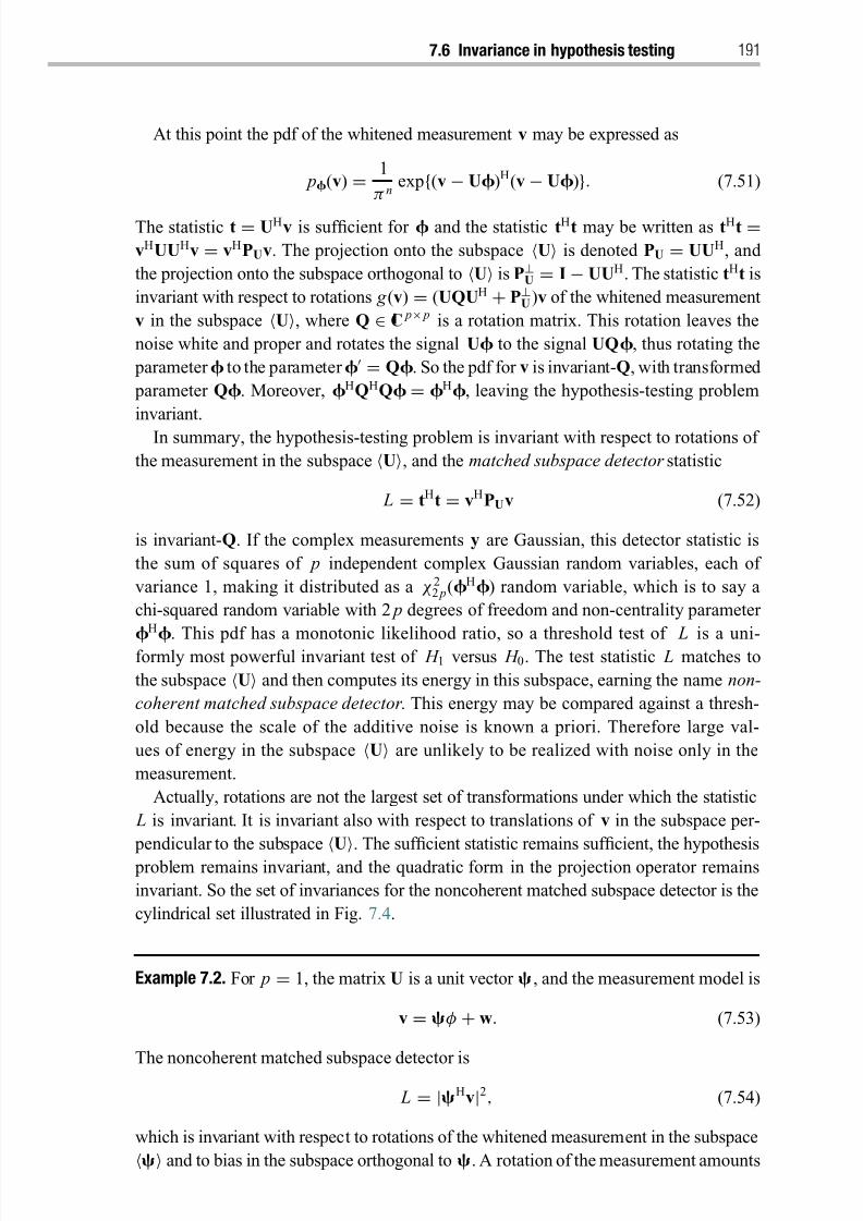
8/21/2019 Statistical Signal Processing of Complex-Valued Data.pdf
http://slidepdf.com/reader/full/statistical-signal-processing-of-complex-valued-datapdf 213/330
7.6 Invariance in hypothesis testing 191
At this point the pdf of the whitened measurement v may be expressed as
p(v) = 1
π n exp{(v − U)H(v − U)}. (7.51)
The statistic t = UHv is sufficient for and the statistic tHt may be written as tHt =vHUUHv = vHPUv. The projection onto the subspace U is denoted PU = UUH, and
the projection onto the subspace orthogonal to U is P⊥U = I − UUH. The statistic tHt is
invariant with respect to rotations g (v) = (UQUH + P⊥U)v of the whitened measurement
v in the subspace U, where Q ∈ C p× p is a rotation matrix. This rotation leaves the
noise white and proper and rotates the signal U to the signal UQ, thus rotating the
parameter to the parameter = Q. So the pdf for v is invariant-Q, with transformed
parameter Q. Moreover, HQHQ = H, leaving the hypothesis-testing problem
invariant.
In summary, the hypothesis-testing problem is invariant with respect to rotations of
the measurement in the subspace U, and the matched subspace detector statistic
L = tHt = vHPUv (7.52)
is invariant-Q. If the complex measurements y are Gaussian, this detector statistic is
the sum of squares of p independent complex Gaussian random variables, each of
variance 1, making it distributed as a χ 22 p(H) random variable, which is to say a
chi-squared random variable with 2 p degrees of freedom and non-centrality parameter
H
. This pdf has a monotonic likelihood ratio, so a threshold test of L is a uni-formly most powerful invariant test of H 1 versus H 0. The test statistic L matches to
the subspace U and then computes its energy in this subspace, earning the name non-
coherent matched subspace detector . This energy may be compared against a thresh-
old because the scale of the additive noise is known a priori. Therefore large val-
ues of energy in the subspace U are unlikely to be realized with noise only in the
measurement.
Actually, rotations are not the largest set of transformations under which the statistic
L is invariant. It is invariant also with respect to translations of v in the subspace per-
pendicular to the subspace
U. The sufficient statistic remains sufficient, the hypothesis
problem remains invariant, and the quadratic form in the projection operator remains
invariant. So the set of invariances for the noncoherent matched subspace detector is the
cylindrical set illustrated in Fig. 7.4.
Example 7.2. For p = 1, the matrix U is a unit vector , and the measurement model is
v = φ + w. (7.53)
The noncoherent matched subspace detector is
L = |Hv|2, (7.54)
which is invariant with respect to rotations of the whitened measurement in the subspace
and to bias in the subspace orthogonal to . A rotation of the measurement amounts
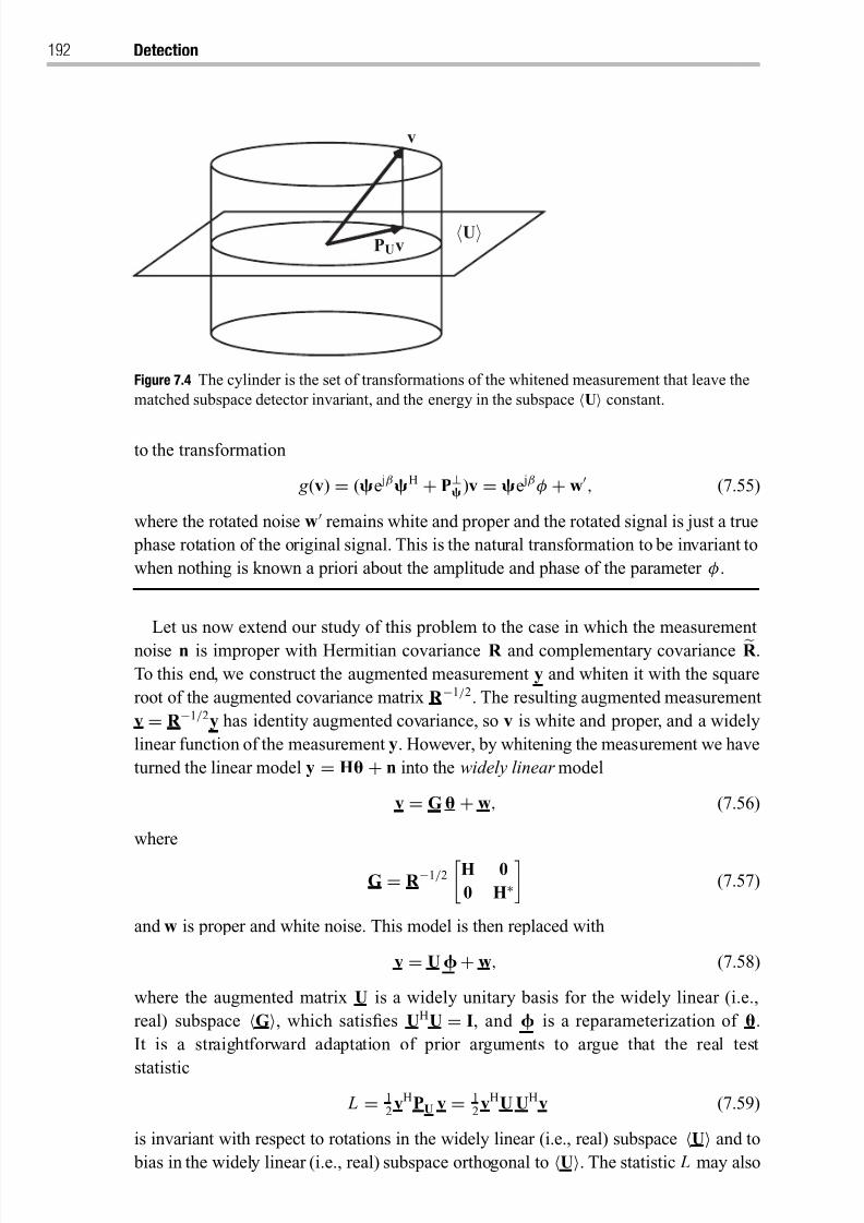
8/21/2019 Statistical Signal Processing of Complex-Valued Data.pdf
http://slidepdf.com/reader/full/statistical-signal-processing-of-complex-valued-datapdf 214/330
192 Detection
PUvU
v
Figure 7.4 The cylinder is the set of transformations of the whitened measurement that leave the
matched subspace detector invariant, and the energy in the subspace U constant.
to the transformation
g (v) = (e jβ H + P⊥ )v = e jβ φ + w, (7.55)
where the rotated noise w remains white and proper and the rotated signal is just a true
phase rotation of the original signal. This is the natural transformation to be invariant to
when nothing is known a priori about the amplitude and phase of the parameter φ .
Let us now extend our study of this problem to the case in which the measurement
noise n is improper with Hermitian covariance R and complementary covariance R .
To this end, we construct the augmented measurement y and whiten it with the square
root of the augmented covariance matrix R −1/2. The resulting augmented measurement
v = R −1/2y has identity augmented covariance, so v is white and proper, and a widely
linear function of the measurement y. However, by whitening the measurement we have
turned the linear model y = H + n into the widely linear model
v = G + w, (7.56)
where
G = R −1/2H 0
0 H∗
(7.57)
and w is proper and white noise. This model is then replaced with
v = U + w, (7.58)
where the augmented matrix U is a widely unitary basis for the widely linear (i.e.,
real) subspace G, which satisfies UHU = I, and is a reparameterization of .
It is a straightforward adaptation of prior arguments to argue that the real test
statistic
L = 12
vHPU v = 12
vHU UHv (7.59)
is invariant with respect to rotations in the widely linear (i.e., real) subspace U and to
bias in the widely linear (i.e., real) subspace orthogonal to U. The statistic L may also
8/21/2019 Statistical Signal Processing of Complex-Valued Data.pdf
http://slidepdf.com/reader/full/statistical-signal-processing-of-complex-valued-datapdf 215/330
7.6 Invariance in hypothesis testing 193
U
v
P⊥U v
PUv
Figure 7.5 The double cone is the set of transformations of the whitened measurement that leave
the CFAR matched subspace detector invariant, and leave the angle that the measurement makeswith the subspace U constant.
be written in terms of v and the components of
U =
U1 U2
U∗2 U∗
1
(7.60)
as
L = vH(U1UH1 + U2UH
2 )v + Re {vT(U∗1UH
2 + U∗2UH
1 )v}. (7.61)
In the proper case, U2 = 0 and U1 = U, so L simplifies to (7.52). If the complex
measurement y is Gaussian, the statistic L is distributed as a χ 22 p(H) random variable.
This is the same distribution as in the proper case – the fact that L is coded as a
real-valued widely quadratic form does not change its distribution.
7.6.2 CFAR matched subspace detector
Thearguments for a constant-false-alarm-rate (CFAR)matched subspacedetector follow
along lines very similar to the lines of argument for the matched subspace detector. The
essential difference is this: the scale of the improper noise is unknown, so the Hermitiancovariance and the complementary covariance are known only up to a nonnegative
scale. That is, σ 2R and σ 2R are the Hermitian and complementary covariances, with
R and R known, but σ 2 > 0 unknown. We ask for invariance with respect to one more
transformation, namely scaling of the measurement by a nonzero constant, which would
have the effect of scaling the variance of the noise and scaling the value of the subspace
parameter , while leaving thehypothesis-testing problem invariant. For proper complex
noise, the statistic
L =vHPU v
vHP⊥U v (7.62)
is invariant with respect to rotations in the widely linear (i.e., real) subspaces U and
U⊥, and to scaling by a nonzero constant. The set of measurements g (v) with respect to
which the statistic L is invariant is illustrated in Fig. 7.5. This invariant set demonstrates
8/21/2019 Statistical Signal Processing of Complex-Valued Data.pdf
http://slidepdf.com/reader/full/statistical-signal-processing-of-complex-valued-datapdf 216/330
194 Detection
that it is the angle that a measurement makes with a subspace that matters, not its energy
in that subspace. The statistic L measures this angle. This is sensible when the scale of
the noise is unknown. That is, L normalizes the energy resolved in the subspace Uwith an estimate of noise power. Since L is the ratio of two independent χ 2 statistics, it
is within a constant of an F -distributed random variable, with 2 p and 2(n − p) degrees
of freedom, and non-centrality parameter H.
Notes
1 There is a comprehensive library of textbooks and research papers on detection theory, which
we make no attempt to catalog. What we have reviewed in this chapter is just a sample of
what seems relevant to detection in the improper Gaussian model, a topic that has not received
much attention in the literature. Even regarding that, we have said nothing about extensionsof detection theory to a theory of adaptive detection that aims to resolve hypotheses when the
subspace is a priori unknown or the covariance matrix of the noise is unknown. The study
of these problems, in the case of proper noise, began with the seminal work of Reed et al .
(1974), Kelly (1986), and Robey et al . (1992), and has seen its most definitive conclusions in
the work of Kraut and Scharf and their collaborators (see Kraut et al . (2001)) and Conte and his
collaborators (see Conte et al . (2001)).
2 The Neyman–Pearson lemma, the Fisher–Neyman factorization theorem, and the Karlin–Rubin
theorem are proved in most books on hypothesis testing and decision theory. Proofs are con-
tained, for instance, in Ferguson (1967). These fundamental theorems are used in Chapter 4 of
Scharf (1991) to derive a number of uniformly most powerful and uniformly most powerful
invariant detectors for real-valued signals.3 This result is originally due to Van Trees (see Van Trees (2001), where it is proved using a
moment-matching argument).
4 The theory of invariance in hypothesis testing is covered comprehensively by Ferguson (1967)
and applied to problems of bias and scale by Scharf (1991).
5 The results in this chapter for matched subspace detectorsgeneralize the results of Scharf (1991)
and Scharf and Friedlander (1994) from real-valued signals to complex-valued signals that may
be proper or improper. Moreover, the adaptive versions of these matched subspace detectors,
termed ada ptive subspace detectors, may be derived, along the lines of papers by Kraut et al .
(2001) and Conte et al . (2001). Adaptive subspace detectors use sample covariance matrices.
These ideas can be generalized further to the matched direction detectors introduced by Besson
et al . (2005).
There is also a body of results addressed to the problem of testing for covariance structure. In
this case the hypothesis is composite, consisting of covariance matrices of specified structure,
and the alternative is composite, consisting of all Hermitian covariance matrices. A selection of
these problems has been addressed in Section 4.5.

8/21/2019 Statistical Signal Processing of Complex-Valued Data.pdf
http://slidepdf.com/reader/full/statistical-signal-processing-of-complex-valued-datapdf 217/330
Part III
Complex random processes

8/21/2019 Statistical Signal Processing of Complex-Valued Data.pdf
http://slidepdf.com/reader/full/statistical-signal-processing-of-complex-valued-datapdf 218/330
8/21/2019 Statistical Signal Processing of Complex-Valued Data.pdf
http://slidepdf.com/reader/full/statistical-signal-processing-of-complex-valued-datapdf 219/330
8 Wide-sense stationary processes
The remaining chapters of the book deal with complex-valued random processes. In
this chapter, we discuss wide-sense stationary (WSS) signals. In Chapter 9, we look at
nonstationary signals, and in Chapter 10, we treat cyclostationary signals, which are an
important subclass of nonstationary signals.
Our discussion of WSS signals continues the preliminary exposition given in Sec-
tion 2.6. WSS processes have shift-invariant second-order statistics, which leads to the
definition of a time-invariant power spectral density (PSD) – an intuitively pleasing idea.
For improper signals, the PSD needs to be complemented by the complementary power
spectral density (C-PSD), which is generally complex-valued. In Section 8.1, we will see
that WSS processes allow an easy characterization of all possible PSD/C-PSD pairs and
also a spectral representation of the process itself. Section 8.2 discusses widely linear
shift-invariant filtering, with an application to analytic and complex baseband signals.
We also introduce the noncausal widely linear minimum mean-squared error, or Wiener,
filter for estimating a message signal from a noisy measurement. In order to find the
causal approximation of the Wiener filter, we need to adapt existing spectral factoriza-
tion algorithms to the improper case. This is done in Section 8.3, where we build causal
synthesis, analysis, and Wiener filters for improper WSS vector-valued time series.
Section 8.4 introduces rotary-component and polarization analysis, which are widely
used in a number of research areas, ranging from optics, geophysics, meteorology, and
oceanography to radar. These techniques are usually applied to deterministic signals,
but we present them in a more general stochastic framework. The idea is to represent
a two-dimensional signal in the complex plane as a superposition of ellipses, whichcan be analyzed in terms of their shape and orientation. Each ellipse is the sum of a
counterclockwise and a clockwise rotating phasor, called the rotary components. If there
is complete coherence between the rotary components (i.e., they are linearly dependent),
then the signal is completely polarized.
Thechapter is concluded with a brief exposition of higher-order statistics of N th-order
stationary signals in Section 8.5, where we focus on higher-order moment spectra and
the principal domains of analytic signals.
8.1 Spectral representation and power spectral density
Consider a zero-mean wide-sense stationary (WSS) continuous-time complex-valued
random process x(t ) = u(t ) + jv(t ), which is composed from the two real random
8/21/2019 Statistical Signal Processing of Complex-Valued Data.pdf
http://slidepdf.com/reader/full/statistical-signal-processing-of-complex-valued-datapdf 220/330
198 Wide-sense stationary processes
processes u(t ) and v(t ) defined for all t ∈ IR. Let us first recall a few key defini-
tions and results from Section 2.6. The process x(t ) is WSS if and only if both
the covariance function r x x (τ ) = E [ x(t + τ ) x∗(t )] and the complementary covari-
ance function r x x
(τ )=
E [ x(t +
τ ) x(t )] are independent of t . Equivalently, the auto-
and cross-covariance functions of real and imaginary parts, r uu (τ ) = E [u(t + τ )u(t )],
r vv (τ ) = E [v(t + τ )v(t )], and r uv(τ ) = E [u(t + τ )v(t )], must all be independent of t .
The process x (t ) is proper when r x x (τ ) = 0 for all τ , which means that r uu (τ ) ≡ r vv (τ )
and r uv(τ ) ≡ −r uv(−τ ), and thus r uv(0) = 0.
The Fourier transform of r x x (τ ) is the power spectral density (PSD) P x x ( f ), and
the Fourier transform of r x x (τ ) is the complementary power spectral density (C-PSD) P x x ( f ). Result 2.14 characterizes all possible pairs ( P x x ( f ), P x x ( f )). This result is
easily obtained by considering the augmented signal x(t ) = [ x(t ), x∗(t )]T whose lag-τ
covariance matrix
R x x (τ ) = E [x(t + τ )xH(t )] =
r x x (τ ) r x x (τ )
r ∗ x x (τ ) r ∗ x x (τ )
(8.1)
is the augmented covariance function of x(t ). The Fourier transform of R x x (τ ) is the
augmented PSD matrix
P x x ( f ) =
P x x ( f ) P x x ( f )
P ∗ x x ( f ) P x x (− f )
. (8.2)
This matrix is a valid augmented PSD matrix if and only if it is positive semidefinite,
which is equivalent to, for all f ,
P x x ( f ) ≥ 0, (8.3) P x x ( f ) = P x x (− f ), (8.4)
| P x x ( f )|2 ≤ P x x ( f ) P x x (− f ). (8.5)
Thus, for any pair of L1-functions ( P x x ( f ), P x x ( f )) that satisfy these three conditions,
there exists a WSS random process x(t ) with PSD P x x ( f ) and C-PSD P x x ( f ). Con-versely, the PSD P x x ( f ) and C-PSD P x x ( f ) of any given WSS random process x(t )
satisfy the conditions (8.3) –(8.5). The same conditions hold for a discrete-time process
x[k ] = u[k ] + jv[k ].
The PSD and C-PSD of x(t ) are connected to the PSDs of real and imaginary parts,
P uu ( f ) and P vv ( f ), and the cross-PSD between real and imaginary part, P uv( f ), through
the familiar real-to-complex transformation
T
= 1 j
1 − j , TTH
=THT
=2I, (8.6)
as
P x x ( f ) = T
P uu ( f ) P uv( f )
P ∗uv( f ) P vv ( f )
TH, (8.7)
8/21/2019 Statistical Signal Processing of Complex-Valued Data.pdf
http://slidepdf.com/reader/full/statistical-signal-processing-of-complex-valued-datapdf 221/330
8.1 Spectral representation 199
from which we determine
P x x ( f ) = P uu ( f )+ P vv ( f )+ 2 Im P uv( f ), (8.8)
P x x (− f ) = P uu ( f )+ P vv ( f )− 2 Im P uv( f ), (8.9) P x x ( f ) = P uu ( f )− P vv ( f )+ 2j Re P uv( f ). (8.10)
The PSD and C-PSD provide a statistical description of the spectral properties of x (t ).
But is there a spectral representation of the process x(t ) itself? The following result,
whose proper version is due to Cramer, is affirmative.
Result 8.1. Provided that r x x (τ ) is continuous, a complex second-order random process
x(t ) can be written as
x(t ) = ∞−∞
e j2π f t d ξ ( f ), (8.11)
where ξ ( f ) is a spectral process with orthogonal increments d ξ ( f ) whose second-order
moments are E |d ξ ( f )|2 = P x x ( f )d f and E [d ξ ( f )d ξ (− f )] = P x x ( f )d f .
This result bears comment. The expression (8.11) almost looks like an inverse Fourier
transform. In fact, if the derivative process X ( f ) = d ξ ( f )/d f existed, then X ( f ) would
be the Fourier transform of x (t ). We would then be able to replace d ξ ( f ) in (8.11) with
X ( f )d f , turning (8.11) into an actual inverse Fourier transform. However, X ( f ) can
never be a second-order random process with finite second-order moment if x (t ) is WSS.This is why we have to resort to the orthogonal increments d ξ ( f ). This issue is further
clarified in Section 9.2.
Theprocess ξ ( f ) hasorthogonal increments, whichmeans that E [d ξ ( f 1)d ξ ∗( f 2)] = 0
and E [d ξ ( f 1)d ξ (− f 2)] = 0 for f 1 = f 2. For f 1 = f 2 = f , E |d ξ ( f )|2 = P x x ( f )d f and
E [d ξ ( f )d ξ (− f )] = P x x ( f )d f . The minus sign in the expression for P x x ( f ) is owed to
the fact that the spectral process corresponding to x ∗(t ) is ξ ∗(− f ):
x∗(t ) =
∞
−∞
e j2π f t d ξ ( f )
∗=
∞
−∞
e j2π f t d ξ ∗(− f ). (8.12)
The process x(t ) can be decomposed into two orthogonal and WSS parts as x(t ) = xc(t ) + xd (t ), where xc(t ) belongs to a continuous spectral process ξ c( f ) and xd (t ) to a
purely discontinuous spectral process ξ d ( f ). The spectral representation of xd (t ) reduces
to a countable sum
xd (t ) = ∞−∞
e j2π f t d ξ d ( f ) =
n
C f n e j2π f n t , (8.13)
where { f n} is the set of discontinuities of ξ ( f ). The random variables
C f n = limε→0+[ξ d ( f n + ε) − ξ d ( f n − ε)] (8.14)
are orthogonal in the sense that E [C f n C ∗ f m] = 0 and E [C f n C − f m ] = 0 for n = m. At fre-
quency f n , the process xd (t ) has power E |C f n |2 and complementary power E [C f n C − f n ],
8/21/2019 Statistical Signal Processing of Complex-Valued Data.pdf
http://slidepdf.com/reader/full/statistical-signal-processing-of-complex-valued-datapdf 222/330
200 Wide-sense stationary processes
and thus unbounded power spectral density. The discontinuities { f n} correspond to peri-
odic components of the correlation function r x x (τ ). The process xc(t ) with continuous
spectral process ξ c( f ) has zero power at all frequencies (but nonzero power spectral
density, unless xc(t )
≡0).
Example 8.1. Consider the ellipse
x(t ) = C +e j2π f 0t + C −e− j2π f 0t , (8.15)
where C + and C − are two complex randomvariables. Thespectral process ξ ( f ) is purely
discontinuous:
ξ ( f )=
0, f < − f 0,
C −,
− f 0 ≤ f <
f 0,
C − + C +, f 0 ≤ f .
(8.16)
In Example 1.5 we found that x (t ) is WSS if and only if E [C +C ∗−] = 0, E C 2+ = 0, and
E C 2− = 0, in which case the covariance function is
r x x (τ ) = E |C +|2e j2π f 0τ + E |C −|2e− j2π f 0τ (8.17)
and the complementary covariance function is
r x x (τ ) = 2 E [C +C −]cos(2π f 0τ ). (8.18)
The covariance and complementary covariance are periodic functions of τ . The power of x(t ) at frequency f 0 is E |C +|2, and at − f 0 it is E |C −|2. The complementary power
at ± f 0 is E [C +C −]. The PSD and C-PSD are thus unbounded line spectra:
P x x ( f ) = E |C +|2δ( f − f 0) + E |C −|2δ( f + f 0), (8.19) P x x ( f ) = E [C +C −][δ( f − f 0) + δ( f + f 0)]. (8.20)
Aliasing in the spectral representation of a discrete-timeprocess x [k ] will be discussed
in the context of nonstationary processes in Section 9.2.
8.2 Filtering
The output of a widely linear shift-invariant (WLSI) filter with impulse response
(h1(t ), h2(t )) and input x (t ) is
y(t ) = (h1 ∗ x)(t ) + (h2 ∗ x∗)(t ) =
∞
−∞
[h1(t − τ ) x(τ ) + h2(t − τ ) x∗(τ )]d τ. (8.21)
If x(t ) and y(t ) have spectral representations with orthogonal increments d ξ ( f ) and
d υ( f ), respectively, they are connected as
d υ( f ) = H 1( f )d ξ ( f )+ H 2( f )d ξ ∗(− f ). (8.22)
8/21/2019 Statistical Signal Processing of Complex-Valued Data.pdf
http://slidepdf.com/reader/full/statistical-signal-processing-of-complex-valued-datapdf 223/330
8.2 Filtering 201
This may be written in augmented notation as
d υ( f )
d υ∗(
− f )
=
H 1( f ) H 2( f )
H ∗2 (
− f ) H ∗1 (
− f )
d ξ ( f )
d ξ ∗(
− f )
. (8.23)
We call
H( f ) =
H 1( f ) H 2( f )
H ∗2 (− f ) H ∗1 (− f )
(8.24)
the augmented frequency-response matrix of the WLSI filter. The relationship between
the augmented PSD matrices of x (t ) and y(t ) is
P yy ( f ) = H( f )P x x ( f )HH( f ). (8.25)
In the following, we will take a look at three important (W)LSI filters: the filter con-structing the analytic signal using the Hilbert transform, the noncausal Wiener filter, and
the causal Wiener filter.
8.2.1 Analytic and complex baseband signals
In Section 1.4, we discussed therole of analytic andequivalent complex baseband signals
in communications. In this section, we will investigate properties of random analytic and
complex baseband signals. Let x (t ) = u(t ) + ju(t ) denote theanalytic signal constructed
from the real signal u(t ) and its Hilbert transform u(t ). As discussed in Section 1.4.2, a
Hilbert transformer is a linear shift-invariant (LSI) filter with impulse response h(t ) =1/(π t ) and frequency response H ( f ) = − j sgn( f ). Producing the analytic signal x(t )
from the real signal u(t ) is therefore an LSI operation with augmented frequency-
response matrix
H( f ) =
1 + j H ( f ) 0
0 1 − j H ∗(− f )
=
1 + j H ( f ) 0
0 1 − j H ( f )
, (8.26)
where the second equality is due to H ( f ) = H ∗(− f ). The augmented PSD matrix of
the real input signal u(t ) is
Puu ( f ) =
P uu ( f ) P uu ( f )
P uu ( f ) P uu ( f )
, (8.27)
which is rank-deficient for all frequencies f . The augmented PSD matrix of the analytic
signal x (t ) is
P x x ( f ) = H( f )Puu ( f )HH( f ). (8.28)
With the mild assumption that u(t ) has no DC component, P uu (0) = 0, we obtain the
PSD of x (t )
P x x ( f ) = P uu ( f )+ H ( f ) P uu ( f ) H ∗( f )+ 2 Im { P uu ( f ) H ∗( f )}= 2 P uu ( f )(1+ sgn( f )) = 4( f ) P uu ( f ), (8.29)
8/21/2019 Statistical Signal Processing of Complex-Valued Data.pdf
http://slidepdf.com/reader/full/statistical-signal-processing-of-complex-valued-datapdf 224/330
202 Wide-sense stationary processes
where ( f ) is the unit-step function. The C-PSD is
P x x ( f ) = P uu ( f )− H ( f ) P uu ( f ) H ∗( f )+ 2j Re { P uu ( f ) H ∗( f )} = 0. (8.30)
So the analytic signal constructed from a WSS real signal has zero PSD for negativefrequencies and four times the PSD of the real signal for positive frequencies, and it is
proper . Propriety also follows from the bound (8.5) since
| P x x ( f )|2 ≤ P x x ( f ) P x x (− f ) = 0. (8.31)
There is also a close interplay between wide-sense stationarity andpropriety forequiv-
alent complex baseband signals. As in Section 1.4, let p(t ) = Re { x(t )e j2π f 0t } denote a
real passband signal obtained by complex modulation of the complex baseband signal
x(t ) with bandwidth < f 0. It is easy to see that a complex-modulated signal x (t )e j2π f 0t
is proper if and only if x(t ) is proper. If x(t )e j2π f 0t is the analytic signal obtained from
p(t ), we find the following.
Result 8.2. A real passband signal p(t ) is WSS if and only if the equivalent complex
baseband signal x(t ) is WSS and proper.
An alternative way to prove this is to express the covariance function of p(t ) as
r pp (t , τ ) = Re
r x x (t , τ )e j2π f 0τ + Re
r x x (t , τ )e j2π f 0(2t +τ )
. (8.32)
If r pp (t , τ ) is to be independent of t , we need the covariance function r x x (t , τ ) to be
independent of t and the complementary covariance function r x x (t , τ )
≡0.
We note a subtle difference between analytic signals and complex baseband signals:
while there are no improper WSS analytic signals, improper WSS complex baseband
signals do exist. However, the real passband signal produced from an improper WSS
complex baseband signal is cyclostationary rather than WSS. Result 8.2 is important
for communications because passband thermal noise is modeled as WSS. Hence, its
complex baseband representation is WSS and proper.
8.2.2 Noncausal Wiener filter
The celebrated Wiener filter produces a linear estimate ˆ x(t ) of a message signal x(t )from an observation (or measurement) y(t ) based on the PSD of y(t ), denoted P yy ( f ),
and the cross-PSD between x(t ) and y(t ), denoted P x y( f ). This assumes that x(t ) and
y(t ) are jointly WSS. The estimate ˆ x(t ) is optimal in the sense that it minimizes the
mean-squared error E | ˆ x(t ) − x(t )|2, which is independent of t because x (t ) and y (t ) are
jointly WSS. The frequency response of the noncausal Wiener filter is
H ( f ) = P x y( f )
P yy ( f ). (8.33)
If y(t ) = x(t ) + n(t ), with uncorrelated noise n(t ) of PSD P nn ( f ), then the frequencyresponse is
H ( f ) = P x x ( f )
P x x ( f )+ P nn ( f ). (8.34)
8/21/2019 Statistical Signal Processing of Complex-Valued Data.pdf
http://slidepdf.com/reader/full/statistical-signal-processing-of-complex-valued-datapdf 225/330
8.3 Causal Wiener filter 203
This has an intuitively appealing interpretation: the filter attenuates frequency compo-
nents where the noise is strong compared with the signal.
The extension of the linear Wiener filter to the widely linear Wiener filter for improper
complex signals presents no particular difficulties. The augmented frequency-response
matrix of the noncausal widely linear Wiener filter is
H( f ) = P x y( f )P−1 yy ( f ). (8.35)
Using the matrix-inversion lemma (A1.42) to invert the 2 × 2 matrix P yy ( f ), we
can derive explicit formulae for H 1( f ) and H 2( f ), similarly to the vector case in
Result 5.3.
Example 8.2. If y(t )
= x(t )
+n(t ), where n(t ) is proper, white noise, uncorrelated with
x(t ), with PSD P nn ( f ) = N 0, we obtain
H 1( f ) = P x x ( f )( P x x ( f )+ N 0) − | P x x ( f )|2( P x x ( f )+ N 0)2 − | P x x ( f )|2
,
H 2( f ) = P x x ( f ) N 0
( P x x ( f )+ N 0)2 − | P x x ( f )|2.
It is easy to see that, for
P x x ( f ) = 0, the frequency response simplifies to
H 1( f ) = P x x ( f )
P x x ( f )+ N 0 and H 2( f ) = 0.
8.3 Causal Wiener filter
The Wiener filter derived above is not suitable for real-time applications because it is
noncausal. In this section, we find the causal Wiener filter for an improper WSS vector-
valued time series. This requires the spectral factorization of an augmented PSD matrix.
We will see that it is straightfor ward to apply existing spectral factorization algorithms
to the improper case, following Spurbeck and Schreier (2007).
8.3.1 Spectral factorization
So far, we have dealt with scalar continuous-time processes. Consider now the zero-
mean WSS vector-valued discrete-time process x[k ] = u[k ] + jv[k ] with matrix-valued
covariance function
R x x [κ] = E x[k + κ]xH
[k ] (8.36)
and matrix-valued complementary covariance functionR x x [κ] = E x[k + κ]xT[k ]. (8.37)
8/21/2019 Statistical Signal Processing of Complex-Valued Data.pdf
http://slidepdf.com/reader/full/statistical-signal-processing-of-complex-valued-datapdf 226/330
204 Wide-sense stationary processes
The augmented matrix covariance function is
R x x [κ] = E x[k + κ]xH[k ] (8.38)
for x[k ] = [xT
[k ], xH
[k ]]T
. It is positive semidefinite for κ = 0 and R x x [κ] = R H x x [−κ].
The augmented PSD matrix P x x (θ ) is the discrete-time Fourier transform (DTFT) of
R x x [κ]. However, in order to spectrally factor P x x (θ ), we need to work with the z -
transform
P x x ( z ) =P x x ( z ) P x x ( z )P∗ x x ( z ∗) P∗ x x ( z ∗)
(8.39)
instead. It satisfies the symmetry property P x x ( z ) = PH x x ( z −∗), and thus P x x ( z ) =
PH x x ( z −∗) and P x x ( z )
= PT x x ( z −1). We indulge in a minor abuse of notation by writ-
ing P x x (θ ) = P x x ( z )| z =e jθ . The augmented PSD matrix P x x (θ ) is positive semidefiniteand Hermitian: P x x (θ ) = PH
x x (θ ).
We wish to factor P x x ( z ) as
P x x ( z ) = A x x ( z )AH x x ( z −∗), (8.40)
where A x x ( z ) is minimum phase, meaning that both A x x ( z ) and A−1 x x ( z ) are causal and
stable.1 This means that both the coloring filter A x x ( z ) and the whitening filter A−1 x x ( z )
haveall their zeros andpoles inside the unit circle. Moreover, sinceA x x ( z ) must represent
a WLSI filter, it needs to satisfy the pattern
A x x ( z ) =A x x ( z ) A x x ( z )A∗
x x ( z ∗) A∗ x x ( z ∗)
. (8.41)
We first determine P zz ( z ) of the real vector time series z[k ] = [uT[k ], vT[k ]]T as
P zz ( z ) = 14
THP x x ( z )T. We will assume that P x x ( z ) and thus also P zz ( z ) are rational,
which means that every element can be written as
[P zz ]i j ( z ) = bi j ( z )
ai j ( z ), (8.42)
where the polynomials bi j ( z ) and ai j ( z ) are coprime with real coefficients. We further
require that no ai j ( z ) have roots on the unit circle. Now we factor P zz ( z ) into a matrix of
polynomials ( z ) divided by a single denominator polynomial α( z ):
P zz ( z ) = 1
α( z )( z ). (8.43)
This factorization is achieved by finding the polynomial α( z ) that is the least common
multiple of all the denominator polynomials {ai j ( z )}. The polynomial α( z ) may be
iteratively computed using Euclid’s algorithm for finding the greatest common divisor
of two polynomials (see, e.g., Blahut (1985)). The elements of ( z ) are then
βi j ( z ) = bi j ( z ) α( z )
ai j ( z ). (8.44)
8/21/2019 Statistical Signal Processing of Complex-Valued Data.pdf
http://slidepdf.com/reader/full/statistical-signal-processing-of-complex-valued-datapdf 227/330
8.4 Rotary-component and polarization analysis 205
Now we factor the polynomial α( z ) to obtain a minimum-phase polynomial α0( z ) such
that α( z ) = α0( z )α0( z −1). Next, we can utilize an efficient algorithm such as the one pro-
vided byJezek andKucera (1985) or Spurbeck andMullis (1998) to factor the polynomial
matrix ( z )=
0( z )T
0( z
−1) with
0( z ) minimum phase. Note that α
0( z
−1)=
α∗0( z
−∗)
and T0 ( z −1) = H
0 ( z −∗) because the polynomials in α( z ) and ( z ) have real coefficients.
Then, 0( z )/α0( z ) is a rational minimum-phase coloring filter for the real time series
z[k ]. Thus,
A x x ( z ) = 1√ 2α0( z )
T0( z )TH (8.45)
is a rational minimum-phase coloring filter for the complex time series x[k ]. It is easy
to verify that (8.40) holds for A x x ( z ) given by (8.45).
8.3.2 Causal synthesis, analysis, and Wiener filters
We can now causally synthesize a WSS vector-valued time series x[k ] with desired PSD
matrix P x x (θ ) and C-PSD matrix P x x (θ ) from a complex white vector sequence w[k ]. To
do this, we factor the augmented PSD matrix as P x x ( z ) = A x x ( z )AH x x ( z −∗) as described
above. The z -transform of the synthesized vector time series x[k ] ←→ X( z ) is then
X( z ) = A x x ( z )W( z ) + A x x ( z )W∗( z ∗), (8.46)
where the input w[k ]
←→W( z ) is a complex white and proper vector time series with
Pww(θ ) = I and Pww(θ ) = 0.We can also causally whiten (analyze) a WSS vector time series x[k ]. In augmented
notation, the z -transform of the filter output is
W( z ) = A−1 x x ( z )X( z ). (8.47)
The augmented transfer function of the noncausal Wiener filter that provides the
widely linear MMSE estimate x[k ] of x[k ] from measurements y[k ] is
Hnc( z ) = P x y( z )P−1 yy ( z ). (8.48)
With the factorization P yy ( z ) = A yy ( z )AH yy ( z −∗), the augmented transfer function of thecausal Wiener filter is then
Hc( z ) = P x y( z )A−H yy ( z −∗)
+A
−1 yy ( z ), (8.49)
where [·]+ denotes the causal part. The z -transform of the estimate is given in augmented
notation by X( z ) = Hc( z )Y( z ).
8.4 Rotary-component and polarization analysis
Rotary-component and polarization analysis are widely used in many research areas,
including optics, geophysics, meteorology, oceanography, and radar.2 The idea is to
represent a two-dimensional signal in the complex plane as an integral of ellipses, and
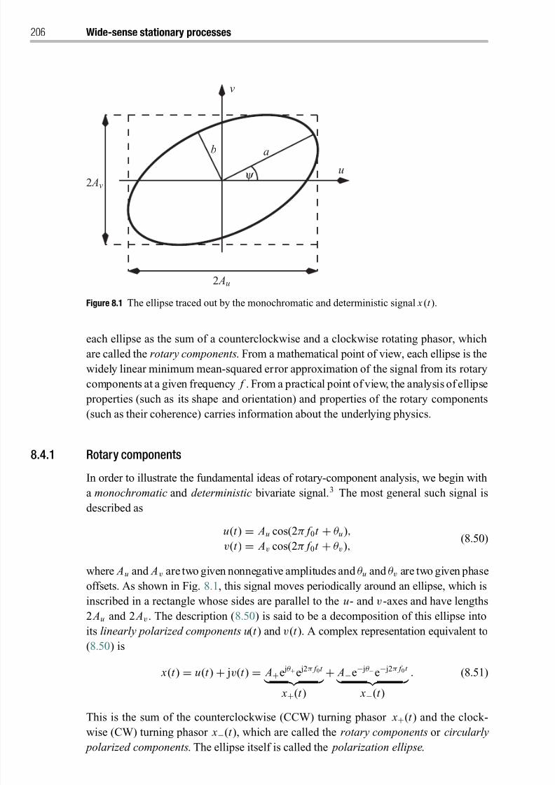
8/21/2019 Statistical Signal Processing of Complex-Valued Data.pdf
http://slidepdf.com/reader/full/statistical-signal-processing-of-complex-valued-datapdf 228/330
206 Wide-sense stationary processes
2 Au
b a
y 2 Av
v
u
Figure 8.1 The ellipse traced out by the monochromatic and deterministic signal x (t ).
each ellipse as the sum of a counterclockwise and a clockwise rotating phasor, which
are called the rotary components. From a mathematical point of view, each ellipse is the
widely linear minimum mean-squared error approximation of the signal from its rotary
components at a given frequency f . From a practical point of view, the analysis of ellipse
properties (such as its shape and orientation) and properties of the rotary components
(such as their coherence) carries information about the underlying physics.
8.4.1 Rotary components
In order to illustrate the fundamental ideas of rotary-component analysis, we begin with
a monochromatic and deterministic bivariate signal.3 The most general such signal is
described as
u(t ) = Au cos(2π f 0t + θ u),
v(t ) = Av cos(2π f 0t + θ v),
(8.50)
where Au and Av are two given nonnegative amplitudes and θ u and θ v are two given phase
offsets. As shown in Fig. 8.1, this signal moves periodically around an ellipse, which is
inscribed in a rectangle whose sides are parallel to the u- and v-axes and have lengths
2 Au and 2 Av . The description (8.50) is said to be a decomposition of this ellipse into
its linearly polarized components u(t ) and v(t ). A complex representation equivalent to
(8.50) is
x(t ) = u(t ) + jv(t ) = A+e jθ +e j2π f 0t
x+(t )
+ A−e− jθ −e− j2π f 0t
x−(t )
. (8.51)
This is the sum of the counterclockwise (CCW) turning phasor x+(t ) and the clock-
wise (CW) turning phasor x−(t ), which are called the rotary components or circularly
polarized components. The ellipse itself is called the polarization ellipse.
8/21/2019 Statistical Signal Processing of Complex-Valued Data.pdf
http://slidepdf.com/reader/full/statistical-signal-processing-of-complex-valued-datapdf 229/330
8.4 Rotary-component and polarization analysis 207
The real description (8.50) and complex description (8.51) can be related through
their PSD matrices. Restricted to nonnegative frequencies f , the PSD matrix of the
vector z(t ) = [u(t ), v(t )]T is
P zz ( f ) = 14 A
2u Au Ave
jθ
Au Ave− jθ A2v
δ( f − f 0), (8.52)
with θ = θ u − θ v . Since P zz ( f ) = P∗ zz (− f ), the PSDs of positive and negative frequen-
cies are trivially related and the restriction to nonnegative frequencies f presents no loss
of information. The augmented PSD matrix for the complex description is
P x x ( f ) =
A2+ A+ A−e j2ψ
A+ A−e− j2ψ A2−
δ( f − f 0), (8.53)
with 2ψ = θ + − θ −. The PSD matrices P zz ( f ) and P x x ( f ) are connected through the
real-to-complex transformation T as
P x x ( f ) = TP zz ( f )TH, (8.54)
from which we obtain the following expressions:
A2+ + A2
− = A2
u + A2v
2 , (8.55)
A2+ − A2
− = Au Av sin θ , (8.56)
tan(2ψ) = 2 Au Av cos θ
A2u − A2
v
= Im{ A+ A−e j2ψ}Re{ A+ A−e j2ψ} . (8.57)
Thus, the ellipse is parameterized by either ( Au , Av , θ ) or ( A+, A−, ψ). If the reader
suspects that the latter will turn out to be more useful, then he or she is right.
We have already determined in Section 1.3 that ψ = (θ + − θ −)/2 is the angle
between the major axis and the u-axis, simply referred to as the orientation of the
ellipse. Moreover, we found that 2a = 2( A+ + A−) is the length of the major axis and
2b = 2| A+ − A−| the lengthof the minor axis. From this, we obtain the areaof the ellipse
abπ = ( A+ + A−)| A+ − A−|π = | A2+ − A2
−|π. (8.58)
The numerical eccentricity
√ a2 − b2
a= 2√ A+ A−
A+ + A−(8.59)
is seen to be the ratio of geometric mean to arithmetic mean of A+ and A−. In optics,
it is common to introduce another angle χ through
sin(2χ) = ± 2ab
a2 + b2 = A2
+ − A2−
A2+ + A2−, −π
4 ≤ χ ≤ π
4, (8.60)
where the expression in the middle is the ratio of geometric mean to arithmetic mean
of a2 and b2, and its sign indicates the rotation direction of the ellipse: CCW for “+
”
and CW for “−.” Because
tan χ = ±b
a= A+ − A−
A+ + A−(8.61)
we may say that χ characterizes the scale-invariant shape of the ellipse.
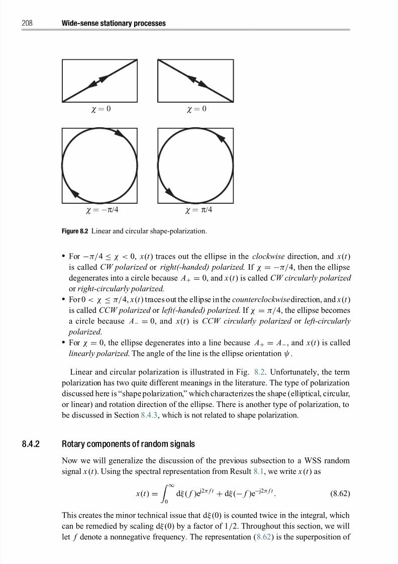
8/21/2019 Statistical Signal Processing of Complex-Valued Data.pdf
http://slidepdf.com/reader/full/statistical-signal-processing-of-complex-valued-datapdf 230/330
208 Wide-sense stationary processes
c = 0
c = π/4 c =−π/4
c = 0
Figure 8.2 Linear and circular shape-polarization.
For −π/4 ≤ χ < 0, x(t ) traces out the ellipse in the clockwise direction, and x(t )
is called CW polarized or right(-handed) polarized . If χ = −π/4, then the ellipse
degenerates into a circle because A+ = 0, and x (t ) is called CW circularly polarized
or right-circularly polarized . For 0 < χ ≤ π/4, x (t ) traces out the ellipse in the counterclockwisedirection, and x (t )
is called CCW polarized or left(-handed) polarized . If χ = π/4, the ellipse becomes
a circle because A− = 0, and x(t ) is CCW circularly polarized or left-circularly
polarized . For χ = 0, the ellipse degenerates into a line because A+ = A−, and x(t ) is called
linearly polarized . The angle of the line is the ellipse orientation ψ .
Linear and circular polarization is illustrated in Fig. 8.2. Unfortunately, the term
polarization has two quite different meanings in the literature. The type of polarization
discussed here is “shape polarization,” which characterizes the shape (elliptical, circular,or linear) and rotation direction of the ellipse. There is another type of polarization, to
be discussed in Section 8.4.3, which is not related to shape polarization.
8.4.2 Rotary components of random signals
Now we will generalize the discussion of the previous subsection to a WSS random
signal x (t ). Using the spectral representation from Result 8.1, we write x (t ) as
x(t ) = ∞0
d ξ ( f )e j2π f t
+ d ξ (− f )e− j2π f t
. (8.62)
This creates the minor technical issue that d ξ (0) is counted twice in the integral, which
can be remedied by scaling d ξ (0) by a factor of 1/2. Throughout this section, we will
let f denote a nonnegative frequency. The representation (8.62) is the superposition of
8/21/2019 Statistical Signal Processing of Complex-Valued Data.pdf
http://slidepdf.com/reader/full/statistical-signal-processing-of-complex-valued-datapdf 231/330
8.4 Rotary-component and polarization analysis 209
ellipses, and one ellipse
ε f (t ) = d ξ ( f )e j2π f t
ε f +(t )
+ d ξ (− f )e− j2π f t
ε f −(t )
(8.63)
can be constructed for a given frequency f ≥ 0. We emphasize that the ellipse ε f (t )
and the rotary components ε f +(t ) and ε f − (t ) are WSS random processes. The rotary
components are each individually proper, but the ellipse ε f (t ) is generally improper.
Interpretation of the random ellipse
There is a powerful interpretation of the ellipse ε f (t ). Assume that we wanted to lin-
early estimate the signal x(t ) from the rotary components at a given frequency f , i.e.,
from ε f +(t )
=d ξ ( f )e j2π f t and ε f
−(t )
=d ξ (
− f )e− j2π f t . Because d ξ ( f ) and d ξ ∗(
− f )
are generally correlated, meaning that P x x ( f )d f = E [d ξ ( f )d ξ (− f )] may be nonzero,
we have the foresight to use a widely linear estimator of the form
ˆ x f (t ) = [ H 1( f )d ξ ( f )+ H 2( f )d ξ ∗(− f )]e j2π f t
+ H 1(− f )d ξ (− f )+ H 2(− f )d ξ ∗( f )]e− j2π f t . (8.64)
So, for a fixed frequency f , we need to determine H 1( f ), H 1(− f ), H 2( f ), and H 2(− f )
such that E | ˆ x f (t ) − x(t )|2 (which is independent of t since x (t ) is WSS) is minimized.
To solve this problem, we first note that the vector [d ξ ( f ), d ξ ∗(
− f )] is uncorrelated
with the vector [d ξ (− f ), d ξ ∗( f )] because x (t ) is WSS. This allows us to determine the
pair ( H 1( f ), H 2( f )) independently from the pair ( H 1(− f ), H 2(− f )). In other words,
the WLMMSE estimate ˆ x f (t ) is the sum of
the LMMSE estimate of x (t ) from ε f + (t ) = d ξ ( f )e j2π f t and ε∗ f −(t ) = d ξ ∗(− f )e j2π f t ,
and the LMMSE estimate of x(t ) from ε∗ f +(t ) = d ξ ∗( f )e− j2π f t and ε f −(t ) =
d ξ (− f )e− j2π f t .
The first is E ( x(t )d ξ ∗( f )e− j2π f t ) E ( x(t )d ξ (− f )e− j2π f t )
×
E |d ξ ( f )|2 E (d ξ ( f )d ξ (− f ))
E (d ξ ∗( f )d ξ ∗(− f )) E |d ξ (− f )|2−1
ε f +(t )
ε∗ f −(t )
=
P x x ( f )d f P x x ( f )d f
P x x ( f )d f P x x ( f )d f
P ∗ x x ( f )d f P x x (− f )d f
−1 ε f +(t )
ε∗ f −(t )
(8.65)
= 1 P x x ( f ) P x x (− f )− | P x x ( f )|2
P x x ( f ) P x x (− f )− | P x x ( f )|2
− P x x ( f ) P x x ( f )+ P x x ( f ) P x x ( f )T ε f + (t )
ε∗ f − (t )
(8.66)
= ε f + (t ). (8.67)
8/21/2019 Statistical Signal Processing of Complex-Valued Data.pdf
http://slidepdf.com/reader/full/statistical-signal-processing-of-complex-valued-datapdf 232/330
210 Wide-sense stationary processes
In (8.65) we have used
E ( x(t )d ξ ∗( f )e− j2π f t ) = E
∞−∞
d ξ (ν)e j2π νt
d ξ ∗( f )e− j2π f t
= E |d ξ ( f )|2 = P x x ( f )d f , (8.68)
E ( x(t )d ξ (− f )e− j2π f t ) = E
∞−∞
d ξ (ν)e j2π νt
d ξ (− f )e− j2π f t
= E (d ξ ( f )d ξ (− f )) = P x x ( f )d f , (8.69)
which hold because ξ ( f ) has orthogonal increments, i.e., E [d ξ (ν)d ξ ∗( f )] = 0 and
E [d ξ (ν)d ξ (− f )] = 0 for ν = f .
A completely analogous computation to (8.66) –(8.67) shows that the LMMSE esti-
mate of x(t ) from ε∗ f + (t ) and ε f − (t ) is simply ε f −(t ). All of this taken together meansthat
ˆ x f (t ) = ε f (t ) = ε f +(t ) + ε f −(t ), (8.70)
i.e., H 1( f ) = H 1(− f ) = 1 and H 2( f ) = H 2(− f ) = 0. This says that the ellipse ε f (t )
in (8.63) is actually the best widely linear estimate of x (t ) that may be constructed from
the rotary components at a given frequency f . Moreover, the widely linear estimate
turns out to be strictly linear. That is, even if the rotary components ε f + (t ) and ε f −(t )
have nonzero complementary correlation, it cannot be exploited to build a widely linear
estimator with smaller mean-squared error than a strictly linear estimator.
Statistical properties of the random ellipse
The second-order statistical properties of the WSS random ellipse ε f (t ) can be approx-
imately determined from the augmented PSD matrix P x x ( f ). From (8.58), we approxi-
mate the expected area of the random ellipse as
π | P x x ( f )− P x x (− f )|d f . (8.71)
This is a crude approximation because it involves exchanging the orderof the expectation
operator and the absolute value. The expected rotation direction of the ellipse is given
by the sign of P x x ( f )− P x x (− f ), where “+” indicates CCW and “−” CW direction.
The angle ψ ( f ), obtained as half the phase of the C-PSD through
tan(2ψ( f )) = Im P x x ( f )
Re P x x ( f ), (8.72)
gives an approximation of the expected ellipse orientation. Similarly, χ( f ) obtained
through
sin(2χ( f ))
=
P x x ( f )− P x x (− f )
P x x ( f )+ P x x (− f )
(8.73)
approximates the expected ellipse shape. The approximations (8.72) and (8.73) are
derived from (8.57) and (8.60), respectively, by applying the expectation operator to the
numerator and denominator separately, thus ignoring the fact that these are generally
8/21/2019 Statistical Signal Processing of Complex-Valued Data.pdf
http://slidepdf.com/reader/full/statistical-signal-processing-of-complex-valued-datapdf 233/330
8.4 Rotary-component and polarization analysis 211
correlated, and exchanging the order of the expectation operator and the sin or tan
function. However, it was shown by Rubin-Delanchy and Walden (2008) that, in the
Gaussian case, ψ ( f ) is the mean ellipse orientation – not just an approximation.
The properties of the ellipse all depend on the PSD and C-PSD, which we have defined
as ensemble averages. In most practical applications, only one realization of a random
process is available. Assuming that the random process is ergodic (which is often a
reasonable assumption), all ensemble averages can be replaced by time averages.
8.4.3 Polarization and coherence
Definition 8.1. Let x(t ) be a WSS complex random process x(t ) with augmented PSD
matrix P x x ( f ) , and let 1( f ) and 2( f ) denote the two real eigenvalues of P x x ( f ) ,
assuming 1( f )≥
2( f ). The degree of polarization of x(t ) at frequency f is defined
as
( f ) = 1( f )− 2( f )
1( f )+ 2( f ), (8.74)
which satisfies 0 ≤ ( f ) ≤ 1. If ( f ) = 0 , then x(t ) is called unpolarized at frequency
f . If ( f ) = 1 , then x(t ) is called completely polarized at frequency f .
We need to emphasize again that there are two meanings of the term polarization: one
is this definition and the other is “shape polarization” as discussed in Section 8.4.1. A
signal that is polarized in the sense of Definition 8.1 does not have to be polarized in the
sense that the shape of the ellipse degenerates into a line or circle, which is called linear
or circular polarization. Similarly, a linearly or circularly polarized signal does not have
to be polarized in the sense of Definition 8.1 either.
The degree of polarization has an intricate relationship with and is in fact sometimes
confused with the magnitude-squared coherence between the CCW and CW rotary
components. “Coherence” is a synonymous term for correlation coefficient, but, in
the frequency domain, “coherence” is much more commonly used than “correlation
coefficient.” In the terminology of Chapter 4, the coherence defined in the following
would be called a reflectional correlation coefficient .
Definition 8.2. The complex coherence between CCW and CW rotary components is
ρ x x ( f ) = E [d ξ ( f )d ξ (− f )] E |d ξ ( f )|2 E |d ξ (− f )|2
= P x x ( f )√
P x x ( f ) P x x (− f ). (8.75)
If either P x x ( f ) = 0 or P x x (− f ) = 0 , then we define ρ x x ( f ) = 1.
We usually consider only the magnitude-squared coherence |ρ x x ( f )|2, which satis-
fies |
ρ x x ( f )|2 ≤ 1. If and only if x(t ) is completely polarized at f , then 2( f ) = 0,
| P x x ( f )|2
= P x x ( f ) P x x (
− f ), and thus det P x x ( f )
=0. We thus find the following con-
nection between the degree of polarization and the magnitude-squared coherence.
Result 8.3. A WSS complex random process x(t ) is completely polarized at frequency f ,
i.e., ( f ) = 1 , if and only if ρ x x ( f ) = 1. The corresponding ellipse ε f (t ) has complete
8/21/2019 Statistical Signal Processing of Complex-Valued Data.pdf
http://slidepdf.com/reader/full/statistical-signal-processing-of-complex-valued-datapdf 234/330
212 Wide-sense stationary processes
coherence between its CCW and CW rotary components. Provided that P x x (− f ) = 0 ,
we have d ξ ( f ) = c f d ξ ∗(− f ) with probability 1, where the complex constant c f is
c f = P x x
( f )
P x x (− f ) =
P x x
( f ) P ∗ x x ( f ). (8.76)
If x(t ) is completely polarized at f , all sample functions of the random ellipse
ε f (t ) turn in the same direction, which is either clockwise – if −π/4 ≤ χ( f ) < 0,
|c f | < 1 with c f given by (8.76) – or counterclockwise – if 0 < χ( f ) ≤ π/4, |c f | > 1.
Monochromatic deterministic signals are always completely polarized, since their aug-
mented PSD matrix is always rank-deficient. Moreover, all analytic signals are com-
pletely polarized for all f , as is evident from detP x x ( f ) ≡ 0 because P x x ( f ) P x x (− f ) ≡0.
However, ρ x x ( f ) = 0, i.e., P x x ( f ) = 0, is only a necessary but not sufficient condition
for a signal to be unpolarized at f , which requires 1( f ) = 2( f ). In fact, for ρ x x ( f ) =0 the degree of polarization takes on a particularly simple form:
( f ) = P x x ( f )− P x x (− f )
P x x ( f )+ P x x (− f )
= |sin(2χ( f ))| . (8.77)
The additional condition of equal power in the rotary components, P x x ( f )=
P x x (−
f ),
for a signal to be unpolarized at f can thus be visualized as a requirement that the
random ellipse ε f (t ) have no preferred rotation direction.
We can find an expression for the degree of polarization ( f ) by using the formula
(A1.13) for the two eigenvalues of the 2 × 2 augmented PSD matrix:
1,2( f ) = 12 tr P x x ( f )± 1
2
tr 2P x x ( f )− 4det P x x ( f ). (8.78)
By inserting this expression into (8.74), we then obtain
( f ) =
1 − 4det P x x ( f )
tr 2P x x ( f ) , (8.79)
without the need for an explicit eigenvalue decomposition of P x x ( f ).
For a given frequency f , it is possible to decompose any WSS signal x(t ) into a
WSS completely polarized signal p(t ) and a WSS unpolarized signal n(t ) (but this
decomposition is generally different for different frequencies).4 This is achieved by
expanding the eigenvalue matrix as
Λ x x ( f ) = Λ pp ( f )+Λnn ( f ) = 1( f )− 2( f ) 0
0 0
+ 2( f ) 0
0 2( f )
. (8.80)

8/21/2019 Statistical Signal Processing of Complex-Valued Data.pdf
http://slidepdf.com/reader/full/statistical-signal-processing-of-complex-valued-datapdf 235/330
8.4 Rotary-component and polarization analysis 213
The degree of polarization ( f ) at frequency f is thus the ratio of the polarized power
to the total power:
( f )
=
P pol( f )
P tot( f )
. (8.81)
The degree of polarization and the magnitude-squared coherence have one more impor-
tant property.
Result 8.4. The degree of polarization ( f ) and the magnitude-squared coherence
|ρ x x ( f )|2 are both invariant under coordinate rotation, i.e., x(t ) and x(t )e jφ have the
same ( f ) and |ρ x x ( f )|2 for a fixed real angle φ .
This is easy to see. If x (t ) is replaced with x (t )e jφ , the PSD and C-PSD transform as
P x x ( f ) −→ P x x ( f ),
P x x ( f ) −→ P x x ( f )e j2φ .
That is, P x x ( f ) and | P x x ( f )| are invariant under coordinate rotation. It follows that
the ellipse shape χ( f ), the degree of polarization ( f ), and the magnitude-squared
coherence |ρ x x ( f )|2 are all invariant under coordinate rotation. On the other hand, the
ellipse orientation ψ( f ) is covariant under coordinate rotation, i.e., it transforms as
ψ( f ) −→ e jφ ψ( f ).
The invariance property of |
ρ x x ( f )|2 is another key advantage of the rotary component
versus the Cartesian description. It is obviously also possible to define the Cartesian
coherence
ρuv( f ) = P uv( f )√ P uu ( f ) P vv ( f )
(8.82)
as a normalized cross-spectrum between the u- and v-components. However, the Carte-
sian magnitude-squared coherence |ρuv( f )|2 does depend on the orientation of the u-
and v-axes, thus limiting its usefulness.
8.4.4 Stokes and Jones vectors
George G. Stokes introduced a set of four parameters to characterize the state of polar-
ization of partially polarized light. These parameters are closely related to the PSD and
C-PSD.
Definition 8.3. The Stokes vector Σ( f ) = [0( f ), 1( f ), 2( f ), 3( f )]T is defined
as
0( f ) = Ev P x x ( f ) = 12[ P x x ( f )+ P x x (− f )],
1( f ) = Re P x x ( f ),
2( f ) = Im P x x ( f ),
3( f ) = Od P x x ( f ) = 12[ P x x ( f )− P x x (− f )],
where Ev P x x ( f ) and Od P x x ( f ) denote the even and odd parts of P x x ( f ).

8/21/2019 Statistical Signal Processing of Complex-Valued Data.pdf
http://slidepdf.com/reader/full/statistical-signal-processing-of-complex-valued-datapdf 236/330
214 Wide-sense stationary processes
The four real-valued parameters (0( f ), 1( f ), 2( f ), 3( f )) are an equivalent
parameterization of ( P x x ( f ), P x x (− f ), P x x ( f )), where P x x (± f ) is real and P x x ( f )
complex. Hence, the polarization-ellipse properties may be determined fromΣ( f ). The
polarized power is
P pol( f ) =
21( f )+ 2
2 ( f )+ 23 ( f ) =
| P x x ( f )|2 + Od 2 P x x ( f ), (8.83)
and the total power is
P tot( f ) = 0( f ) = Ev P x x ( f ). (8.84)
The degree of polarization (8.79) can thus be expressed as
( f ) = | P x x ( f )|2
+Od 2 P x x ( f )
Ev P x x ( f ) . (8.85)
An unpolarized signal has 1( f ) = 2( f ) = 3( f ) = 0, and a completely polarized
signal has 21( f )+ 2
2( f )+ 23 ( f ) = 2
0( f ). Thus, three real-valued parameters suf-
fice to characterizea completely polarizedsignal. Which threeparameters to choose is,of
course, somewhat arbitrary. The most common way uses ( P uu ( f ), P vv ( f ), arg P uv( f )),
which are combined in the Jones vector
j( f ) = j 1( f )
j 2( f ) = P uu ( f )
P vv ( f )e j arg P uv ( f ). (8.86)
We note that only the angle of the cross-PSD P uv( f ) between the real part u(t ) and the
imaginarypart v(t ) is specified.Themagnitude | P uv( f )| is determinedbythe assumption
that the signal is completely polarized, which means that the determinant of the PSD
matrix P zz ( f ) is zero:
detP zz ( f ) = det
P uu ( f ) P uv( f )
P ∗uv( f ) P vv ( f )
= 0 ⇐⇒ | P uv( f )|2 = P uu ( f ) P vv ( f ). (8.87)
The reason why the Jones vector uses the Cartesian coordinate system rather than
the rotary components is simply historical. It would be just as easy (and maybe moreinsightful) to instead use the three parameters ( P x x ( f ), P x x (− f ), arg P x x ( f )), and fix
the magnitude of the C-PSD as | P x x ( f )|2 = P x x ( f ) P x x (− f ).
On the other hand, we may also express the Stokes vector in the Cartesian
coordinate system as 0( f ) = P uu ( f )+ P vv ( f ), 1( f ) = P uu ( f )− P vv ( f ), 2( f ) =2 Re P uv( f ), and 3( f ) = 2 Im P uv( f ). This allows us to determine equivalent Jones
and Stokes vectors for fully polarized signals. Remember that the Jones vectors cannot
describe partially polarized or unpolarized signals.
The effect of optical elements on Stokes vectors can be described by multiplication
from the left with a real-valued 4 × 4 matrix. This is called the Mueller calculus.For completely polarized light, there exists an analog calculus for manipulation of
Jones vectors, which uses complex-valued 2 × 2 matrices. This is called the Jones
calculus.5
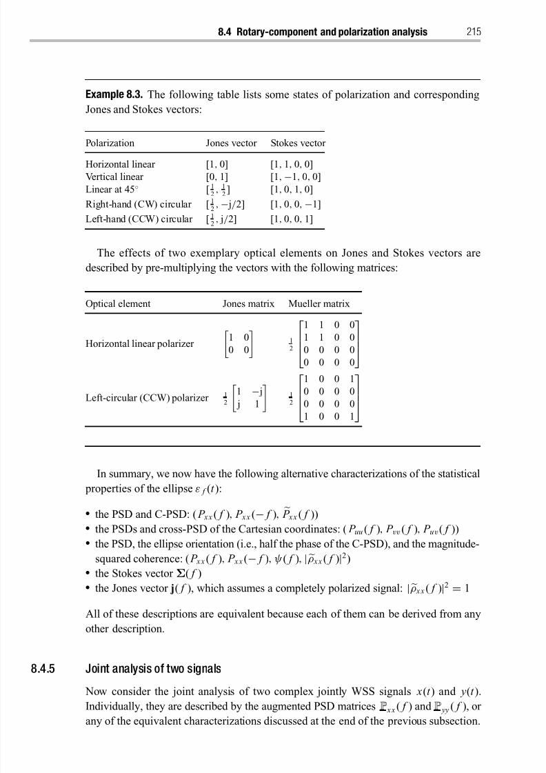
8/21/2019 Statistical Signal Processing of Complex-Valued Data.pdf
http://slidepdf.com/reader/full/statistical-signal-processing-of-complex-valued-datapdf 237/330
8.4 Rotary-component and polarization analysis 215
Example 8.3. The following table lists some states of polarization and corresponding
Jones and Stokes vectors:
Polarization Jones vector Stokes vector
Horizontal linear [1, 0] [1, 1, 0, 0]
Vertical linear [0, 1] [1,−1, 0, 0]
Linear at 45◦ [ 12
, 12] [1, 0, 1, 0]
Right-hand (CW) circular [ 12
,− j/2] [1, 0, 0,−1]
Left-hand (CCW) circular [ 12
, j/2] [1, 0, 0, 1]
The effects of two exemplary optical elements on Jones and Stokes vectors are
described by pre-multiplying the vectors with the following matrices:
Optical element Jones matrix Mueller matrix
Horizontal linear polarizer
1 0
0 0
1
2
1 1 0 0
1 1 0 0
0 0 0 0
0 0 0 0
Left-circular (CCW) polarizer 1
2 1 − j
j 1 12
1 0 0 1
0 0 0 0
0 0 0 01 0 0 1
In summary, we now have the following alternative characterizations of the statistical
properties of the ellipse ε f (t ):
the PSD and C-PSD: ( P x x ( f ), P x x (− f ),
P x x ( f ))
the PSDs and cross-PSD of the Cartesian coordinates: ( P uu ( f ), P vv ( f ), P uv( f ))
the PSD, the ellipse orientation (i.e., half the phase of the C-PSD), and the magnitude-squared coherence: ( P x x ( f ), P x x (− f ), ψ( f ), |ρ x x ( f )|2)
the Stokes vector Σ( f ) the Jones vector j( f ), which assumes a completely polarized signal: |ρ x x ( f )|2 = 1
All of these descriptions are equivalent because each of them can be derived from any
other description.
8.4.5 Joint analysis of two signals
Now consider the joint analysis of two complex jointly WSS signals x(t ) and y(t ).
Individually, they are described by the augmented PSD matrices P x x ( f ) and P yy ( f ), or
any of the equivalent characterizations discussed at the end of the previous subsection.
8/21/2019 Statistical Signal Processing of Complex-Valued Data.pdf
http://slidepdf.com/reader/full/statistical-signal-processing-of-complex-valued-datapdf 238/330
216 Wide-sense stationary processes
Their joint properties are described by the augmented cross-PSD matrix
P x y( f ) =
P x y( f )
P x y( f )
P ∗ x y(
− f ) P ∗ x y(
− f )
, (8.88)
which is the Fourier transform of
R x y(τ ) = E [x(t + τ )yH(t )] =
r x y(τ ) r x y(τ )
r ∗ x y(τ ) r ∗ x y(τ )
. (8.89)
Denoting the spectral process corresponding to y(t ) by υ ( f ), we can express the cross-
PSD and cross-C-PSD as
P x y( f )d f = E [d ξ ( f )d υ∗( f )], (8.90)
P x y( f )d f = E [d ξ ( f )d υ(− f )]. (8.91)
Instead of using the four complex-valued cross-(C-)PSDs P x y( f ), P x y(− f ), P x y( f ), and P x y(− f ) directly, we can also define the magnitude-squared coherences
|ρ x y(± f )|2 = | P x y(± f )|2 P x x (± f ) P yy (± f )
, (8.92)
|
ρ x y(± f )|2 = | P x y(± f )|2
P x x (± f ) P yy (∓ f ), (8.93)
which are rotational and reflectional correlation coefficients, respectively. Let ψ x y(± f )denote the phase of P x y(± f ), and ψ x y(± f ) the phase of P x y(± f ). Then the joint analysis
of x (t ) and y(t ) is performed using the quantities
( P x x (± f ), |ρ x x ( f )|2, ψ x x ( f )) to describe the individual properties of x (t ), ( P yy (± f ), |ρ yy ( f )|2, ψ yy ( f )) to describe the individual properties of y(t ), and (|ρ x y(± f )|2, |ρ x y(± f )|2, ψ x y(± f ), ψ x y(± f )) to describe the joint properties of x(t )
and y(t ).
It is also possible to define a total coherence between x(t ) and y(t ) as a correlation
coefficient between the vectors [d ξ ( f ), d ξ ∗(− f )]T and [d υ( f ), d υ∗(− f )]T. This would proceed along the lines discussed in Chapter 4.
8.5 Higher-order spectra
So far in this chapter, we have considered only second-order properties. We now look at
higher-order moments of a complex N th-order stationary signal x(t ) that has moments
defined and bounded up to N th order. For n ≤ N , it is possible to define 2n different nth-
order moment functions, depending on where complex conjugate operators are placed:
m x,♦( ) = E
xn (t )
n−1i=1
xi (t + τ i )
. (8.94)
8/21/2019 Statistical Signal Processing of Complex-Valued Data.pdf
http://slidepdf.com/reader/full/statistical-signal-processing-of-complex-valued-datapdf 239/330
8.5 Higher-order spectra 217
In this equation, = [τ 1, . . . , τ n−1]T is a vector of time lags, and ♦ =[n,1,2, . . . ,n−1] has elements i that are either 1 or the conjugating star ∗. For
example, if ♦ = [1, 1, ∗], then m x,♦( ) = m x x x∗(τ 1, τ 2) = E [ x(t ) x(t + τ 1) x∗(t + τ 2)].
The number of stars in ♦ will be denoted by q and the number of 1s by n − q . If x(t )is N th-order stationary, then all moments up to order N are functions of only. It is
possible that some moments do not depend on t , whereas others do. Such a process is
not N th-order stationary.
For n = 2, m x ,♦( ) is a correlation function (Hermitian or complementary), for n = 3
it is a bicorrelation function, and for n = 4 it is a tricorrelation function. Many of the
2n moments obtained for the 2n possible conjugation patterns are redundant. First of all,
moments with the same number of stars are equivalent because they are related to each
other through a simple coordinate transformation. For example,
m x x x∗(τ 1, τ 2) = m x∗ x x (τ 1 − τ 2,−τ 2). (8.95)
Secondly, moments withq stars are related to moments with n − q stars through complex
conjugation and possibly an additional coordinate transformation. For instance,
m x x x∗(τ 1, τ 2) = m∗ x∗ x x∗ (τ 2, τ 1). (8.96)
We call two moments equivalent if they can be expressed in terms of each other, and
distinct if they cannot be expressed in terms of each other. There are n/2 + 1 distinct
nth-order moment functions, where n/2 denotes the greatest integer less than or equal
to n/2. In general, all distinct nth-order moment functions are required for an nth-order
description of x (t ).
Higher-order statistical analysis often uses cumulants rather than moments. For
simplicity, we consider only moments here. However, the extension to cumulants
is straightforward, using the connection between cumulants and moments given in
Section 2.5.
8.5.1 Moment spectra and principal domains
We assume that the spectral process ξ ( f ) corresponding to x (t ) is an N th-order random
function with moments defined and bounded up to N th order. In the following, let i f i
denote − f i if i is the conjugating star ∗. The (n − 1)-dimensional Fourier transform
of m x,♦( ) is the nth-order moment spectrum M x,♦(f ), with f = [ f 1, f 2, . . . , f n−1]T:
M x,♦(f ) =
IR n−1
m x,♦( )e− j2π f T d n−1 . (8.97)
This can be expressed in terms of the increments of the spectral process ξ ( f ) as
M x ,♦(f )d n−1f = E
d ξ n (− n f T1)
n−1
i=1
d ξ i (i f i )
, (8.98)
with 1 = [1, 1, . . . , 1]T and f T1 = f 1 + f 2 + · · · + f n−1. The relationship (8.98) will be
further illuminated in Section 9.5. For n = 2, M x,♦(f ) is a power spectrum (the PSD or
C-PSD), for n = 3 it is a bispectrum, and for n = 4 it is a trispectrum. Which ones of
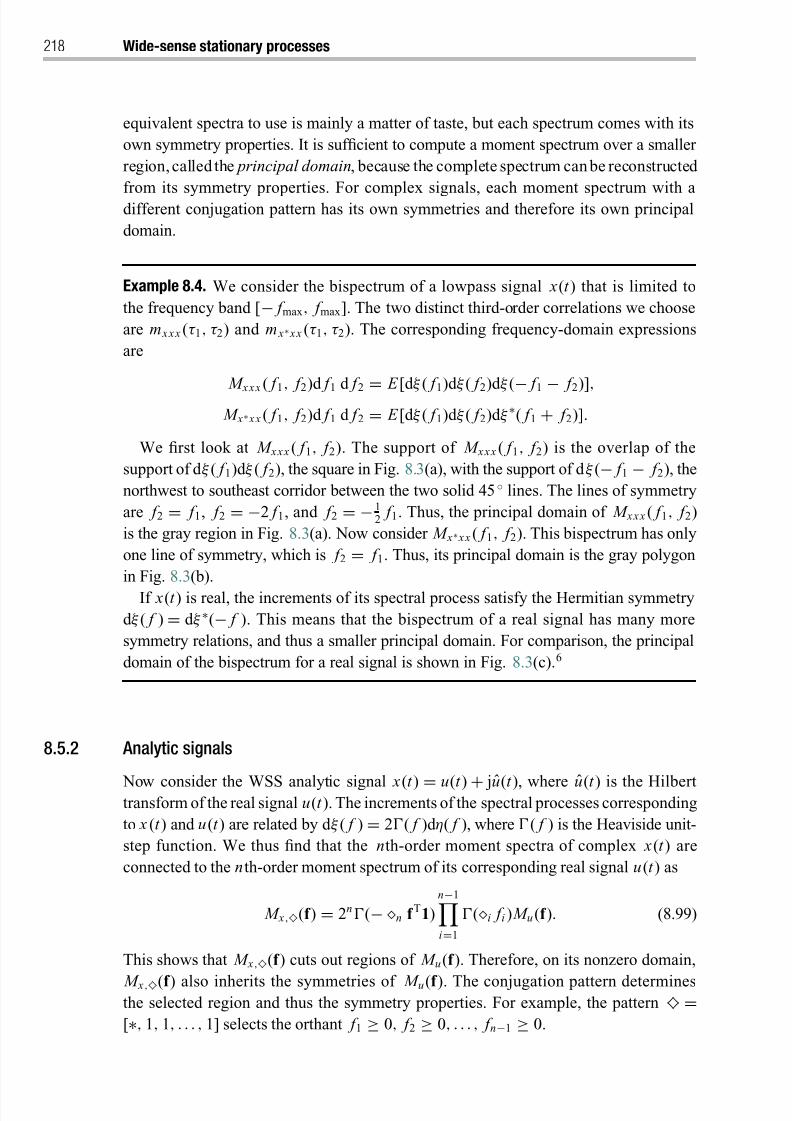
8/21/2019 Statistical Signal Processing of Complex-Valued Data.pdf
http://slidepdf.com/reader/full/statistical-signal-processing-of-complex-valued-datapdf 240/330
218 Wide-sense stationary processes
equivalent spectra to use is mainly a matter of taste, but each spectrum comes with its
own symmetry properties. It is sufficient to compute a moment spectrum over a smaller
region, called the principal domain, because the complete spectrum can be reconstructed
from its symmetry properties. For complex signals, each moment spectrum with a
different conjugation pattern has its own symmetries and therefore its own principal
domain.
Example 8.4. We consider the bispectrum of a lowpass signal x(t ) that is limited to
the frequency band [− f max, f max]. The two distinct third-order correlations we choose
are m x x x (τ 1, τ 2) and m x∗ x x (τ 1, τ 2). The corresponding frequency-domain expressions
are
M x x x
( f 1
, f 2)d f
1 d f
2 = E [d ξ ( f
1)d ξ ( f
2)d ξ (
− f
1 − f
2)],
M x∗ x x ( f 1, f 2)d f 1 d f 2 = E [d ξ ( f 1)d ξ ( f 2)d ξ ∗( f 1 + f 2)].
We first look at M x x x ( f 1, f 2). The support of M x x x ( f 1, f 2) is the overlap of the
support of d ξ ( f 1)d ξ ( f 2), the square in Fig. 8.3(a), with the support of d ξ (− f 1 − f 2), the
northwest to southeast corridor between the two solid 45◦ lines. The lines of symmetry
are f 2 = f 1, f 2 = −2 f 1, and f 2 = − 12
f 1. Thus, the principal domain of M x x x ( f 1, f 2)
is the gray region in Fig. 8.3(a). Now consider M x∗ x x ( f 1, f 2). This bispectrum has only
one line of symmetry, which is f 2 = f 1. Thus, its principal domain is the gray polygon
in Fig. 8.3(b).
If x(t ) is real, the increments of its spectral process satisfy the Hermitian symmetry
d ξ ( f ) = d ξ ∗(− f ). This means that the bispectrum of a real signal has many more
symmetry relations, and thus a smaller principal domain. For comparison, the principal
domain of the bispectrum for a real signal is shown in Fig. 8.3(c).6
8.5.2 Analytic signals
Now consider the WSS analytic signal x(t ) = u(t ) + ju(t ), where u(t ) is the Hilberttransform of the real signal u(t ). The increments of the spectral processes corresponding
to x (t ) and u(t ) are related by d ξ ( f ) = 2( f )d η( f ), where ( f ) is the Heaviside unit-
step function. We thus find that the nth-order moment spectra of complex x(t ) are
connected to the nth-order moment spectrum of its corresponding real signal u(t ) as
M x,♦(f ) = 2n (− n f T1)
n−1i=1
(i f i ) M u(f ). (8.99)
This shows that M x,♦(f ) cuts out regions of M u(f ). Therefore, on its nonzero domain,
M x,♦(f ) also inherits the symmetries of M u(f ). The conjugation pattern determinesthe selected region and thus the symmetry properties. For example, the pattern ♦ =[∗, 1, 1, . . . , 1] selects the orthant f 1 ≥ 0, f 2 ≥ 0, . . . , f n−1 ≥ 0.
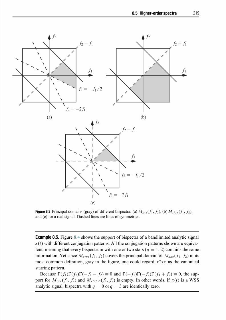
8/21/2019 Statistical Signal Processing of Complex-Valued Data.pdf
http://slidepdf.com/reader/full/statistical-signal-processing-of-complex-valued-datapdf 241/330
8.5 Higher-order spectra 219
(a) (b)
(c)
f 2 = f 1
f 1
f 2 f 2
f 1
f 2 =−
2 f 1
f 2 = f 1
f 2 =−
f 2 =−
f 2 = f 1
f 2 =−2 f 1
f 1
f 2
f 12
f 12
Figure 8.3 Principal domains (gray) of different bispectra: (a) M x x x ( f 1, f 2), (b) M x∗ x x ( f 1, f 2),
and (c) for a real signal. Dashed lines are lines of symmetries.
Example 8.5. Figure 8.4 shows the support of bispectra of a bandlimited analytic signal
x(t ) with different conjugation patterns. All the conjugation patterns shown are equiva-
lent, meaning that every bispectrum with one or two stars (q = 1, 2) contains the same
information. Yet since M x∗ x x ( f 1, f 2) covers the principal domain of M x x x ( f 1, f 2) in its
most common definition, gray in the figure, one could regard x∗ x x as the canonical
starring pattern.
Because ( f 1)( f 2)(− f 1 − f 2) ≡ 0 and (− f 1)(− f 2)( f 1 + f 2) ≡ 0, the sup-
port for M x x x ( f 1, f 2) and M x∗ x∗ x∗( f 1, f 2) is empty. In other words, if x(t ) is a WSSanalytic signal, bispectra with q = 0 or q = 3 are identically zero.
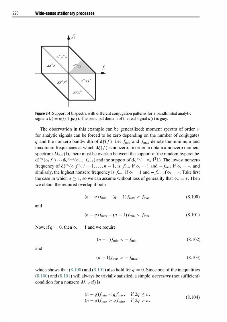
8/21/2019 Statistical Signal Processing of Complex-Valued Data.pdf
http://slidepdf.com/reader/full/statistical-signal-processing-of-complex-valued-datapdf 242/330
220 Wide-sense stationary processes
x∗ xx∗
xxx∗
xx∗ x∗
x∗ xx
x∗ x∗ x xx∗ x
f 2
f 1
Figure 8.4 Support of bispectra with different conjugation patterns for a bandlimited analyticsignal x (t ) = u(t ) + ju(t ). The principal domain of the real signal u(t ) is gray.
The observation in this example can be generalized: moment spectra of order n
for analytic signals can be forced to be zero depending on the number of conjugates
q and the nonzero bandwidth of d ξ ( f ). Let f min and f max denote the minimum and
maximum frequencies at which d ξ ( f ) is nonzero. In order to obtain a nonzero moment
spectrum M x,♦(f ), there must be overlap between the support of the random hypercube
d ξ 1(1 f 1) · · · d ξ n−1(n−1 f n−1) and the support of d ξ n (− n f T1). The lowest nonzero
frequency of d ξ i (
i f i ), i =
1, . . . , n−
1, is f min if
i
=1 and
− f max if
i
= ∗, and
similarly, the highest nonzero frequency is f max if i = 1 and − f min if i = ∗. Take first
the case in which q ≥ 1, so we can assume without loss of generality that n = ∗. Then
we obtain the required overlap if both
(n − q) f min − (q − 1) f max < f max (8.100)
and
(n − q) f max − (q − 1) f min > f min. (8.101)
Now, if q = 0, then n = 1 and we require
(n − 1) f min < − f min (8.102)
and
(n − 1) f max > − f max, (8.103)
which shows that (8.100) and (8.101) also hold for q = 0. Since one of the inequalities
(8.100) and (8.101) will always be trivially satisfied, a simple necessary (not sufficient)
condition for a nonzero M x,♦(f ) is
(n − q) f min < q f max, if 2q ≤ n,
(n − q) f max > q f min, if 2q > n . (8.104)
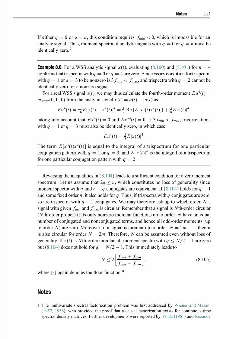
8/21/2019 Statistical Signal Processing of Complex-Valued Data.pdf
http://slidepdf.com/reader/full/statistical-signal-processing-of-complex-valued-datapdf 243/330
Notes 221
If either q = 0 or q = n, this condition requires f min < 0, which is impossible for an
analytic signal. Thus, moment spectra of analytic signals with q = 0 or q = n must be
identically zero.7
Example 8.6. For a WSS analytic signal x(t ), evaluating (8.100) and (8.101) for n = 4
confirmsthat trispectra with q = 0 or q = 4 arezero. A necessary condition for trispectra
with q = 1 or q = 3 to be nonzero is 3 f min < f max, and trispectra with q = 2 cannot be
identically zero for a nonzero signal.
For a real WSS signal u(t ), we may thus calculate the fourth-order moment Eu4(t ) =m x x x x (0, 0, 0) from the analytic signal x (t ) = u(t ) + ju(t ) as
Eu4(t ) = 116
E [ x(t ) + x∗(t )]4 = 12 Re { E [ x 3(t ) x∗(t )]} + 3
8 E | x(t )|4,
taking into account that E x4(t ) = 0 and E x∗4(t ) = 0. If 3 f min > f max, tricorrelationswith q = 1 or q = 3 must also be identically zero, in which case
E u4(t ) = 38 E | x(t )|4.
The term E [ x 3(t ) x∗(t )] is equal to the integral of a trispectrum for one particular
conjugation pattern with q = 1 or q = 3, and E | x(t )|4 is the integral of a trispectrum
for one particular conjugation pattern with q = 2.
Reversing the inequalities in (8.104) leads to a sufficient condition for a zero momentspectrum. Let us assume that 2q ≤ n, which constitutes no loss of generality since
moment spectra with q and n − q conjugates are equivalent. If (8.104) holds for q − 1
and some fixed order n, it also holds for q . Thus, if trispectra with q conjugates are zero,
so are trispectra with q − 1 conjugates. We may therefore ask up to which order N a
signal with given f min and f max is circular. Remember that a signal is N th-order circular
( N th-order proper) if its only nonzero moment functions up to order N have an equal
number of conjugated and nonconjugated terms, and hence all odd-order moments (up
to order N ) are zero. Moreover, if a signal is circular up to order N = 2m − 1, then it
is also circular for order N =
2m. Therefore, N can be assumed even without loss of
generality. If x (t ) is N th-order circular, all moment spectra with q ≤ N /2 − 1 are zero
but (8.104) does not hold for q = N /2 − 1. This immediately leads to
N ≤ 2
f max + f min
f max − f min
, (8.105)
where · again denotes the floor function.8
Notes
1 The multivariate spectral factorization problem was first addressed by Wiener and Masani
(1957, 1958), who provided the proof that a causal factorization exists for continuous-time
spectral density matrices. Further developments were reported by Youla (1961) and Rozanov
8/21/2019 Statistical Signal Processing of Complex-Valued Data.pdf
http://slidepdf.com/reader/full/statistical-signal-processing-of-complex-valued-datapdf 244/330
222 Wide-sense stationary processes
(1963), who provide general algorithms that perform spectral factorization on rational spectral-
density matrices for continuous-time WSS processes. Several spectral-factorization algorithms
for discrete-time spectral-density matrices have been proposed by Davis (1963), Wilson (1972),
and Jezek and Kucera (1985).
2 The seminal paper that first investigated the coherence pro perties of partially polarized lightis Wolf (1959), and an extended discussion is provided by Born and Wolf (1999). The rotar y
component method was introduced in oceanography by Gonella (1972) and Mooers (1973).
Other key papers that deal with polarization and coherence are Jones (1979) and Samson
(1980).
3 The presentation in Section 8.4.1 follows Schreier (2008b). This pa per is cIEEE, and portions
are used with permission. A similar discussion is also provided by Lilly and Gascard (2006).
4 There are other interesting signal decompositions for a given frequency f besides the one into
a completely polarized and an unpolarized signal. Rubin-Delanchy and Walden (2008) present
a decomposition into two ellipses whose orientations are orthogonal, but with the same aspect
ratio. The magnitude-squared coherence between CCW and CW rotary components controls
the relative influences of the two ellipses. If |ρ x x ( f )|2 = 1, then the second ellipse vanishes. If |ρ x x ( f )|2 = 0, then the two ellipses have equal influence.
5 TheStokes parameters were introduced by Stokes (1852), and the Jones parameters and calculus
by Jones (1941). Mueller calculus was invented by Hans Muller (whose last name is commonly
transcribed as “Mueller”) at MITin the early 1940s. Interestingly, the first time Mullerpublished
work using his calculus was only several years later, in Mueller (1948).
6 The symmetry relations of the bispectrum for real signals are detailed by Pflug et al . (1992) and
Molle and Hinich (1995). The bispectrum of complex signals has been discussed by Jouny and
Moses (1992), but they did not consider the bispectrum with no conjugated terms. Higher-or der
spectra with all distinct conjugation patterns were discussed by Schreier and Scharf (2006b).
7 The principal domains of the bispectrum and trispectrum of real signals were derived by Pflug
et al . (1992). Necessary conditions for nonzero moment spectra of analytic signals were given
by Picinbono (1994) and Amblard et al . (1996b). This discussion was extended by Izzo and
Napolitano (1997) to necessary conditions for nonzero spectra of equivalent complex baseband
signals.
8 A thorough discussion of circular random signals, including the interplay between circularity
and stationarity, is provided by Picinbono (1994). The result that connects N th-order circularity
to the bandwidth of analytic signals is also due to Picinbono(1994), and was derived byAmblard
et al . (1996b) as well.
8/21/2019 Statistical Signal Processing of Complex-Valued Data.pdf
http://slidepdf.com/reader/full/statistical-signal-processing-of-complex-valued-datapdf 245/330
9 Nonstationary processes
Wide-sense stationary (WSS) processes admit a spectral representation (see Result 8.1)
in terms of the Fourier basis, which allows a frequency interpretation. The transform-
domain description of a WSS signal x(t ) is a spectral process ξ ( f ) with orthogonal
increments d ξ ( f ). For nonstationary signals, we have to sacrifice either the Fourier
basis, and thus its frequency interpretation, or the orthogonality of the transform-domain
representation. We will discuss both possibilities.
TheKarhunen–Loeve (KL) expansion uses an orthonormal basisother than theFourier
basis but retains the orthogonality of the transform-domain description. The KL expan-
sion is applied to a continuous-time signal of finite duration, which means that its
transform-domain description is a countably infinite number of orthogonal random
coefficients. This is analogous to the Fourier series, which produces a countably infinite
number of Fourier coefficients, as opposed to the Fourier transform, which is applied
to an infinite-duration continuous-time signal. The KL expansion presented in Section
9.1 takes into account the complementary covariance of an improper signal. It can be
considered the continuous-time equivalent of the eigenvalue decomposition of improper
random vectors discussed in Section 3.1.
An alternative approach is the Cramer–Loeve (CL) spectral representation, which
retains the Fourier basis and its frequency interpretation but sacrifices the orthogonality
of the incrementsd ξ ( f ). As discussed in Section 9.2, theincrementsd ξ ( f ) of the spectral
process of an improper signal can have nonzero Hermitian correlation and complemen-
tary correlation between different frequencies. Starting from the CL representation, we
introduce energy and power spectral densities for nonstationary signals. We then discussthe CL representation for analytic signals and discrete-time signals.
Yet another description, which allows deep insights into the time-varying nature of
nonstationary signals, is possible in the joint time–frequency domain. In Section 9.3, we
focus our attention on the Rihaczek distribution, which is a member of Cohen’s class of
bilinear time–frequency distributions. The Rihaczek distribution is not as widely used
as, for instance, the Wigner–Ville distribution, but it possesses a compelling property:
it is an inner product between the spectral increments and the time-domain process at a
given point in the time–frequency plane. This property leads to an evocative geometrical
interpretation. It is also the basis for extending the rotary-component and polarizationanalysis presented in the previous chapter to nonstationary signals. This is discussed in
Section 9.4. Finally, Section 9.5 presents a short exposition of higher-order statistics for
nonstationary signals.
8/21/2019 Statistical Signal Processing of Complex-Valued Data.pdf
http://slidepdf.com/reader/full/statistical-signal-processing-of-complex-valued-datapdf 246/330
224 Nonstationary processes
9.1 Karhunen–Lo eve expansion
We first consider a representation for finite-length continuous-time signals. Like the
Fourier series, this representation produces a countably infinite number of uncorre-lated random coefficients. However, because it uses an orthonormal basis other than
the Fourier basis it generally does not afford these random coefficients a frequency-
domain interpretation. The improper KL expansion is the continuous-time equiva-
lent of the finite-dimensional improper eigenvalue decomposition, which is given in
Result 3.1.1
Result 9.1. Suppose that { x(t ) , 0 ≤ t ≤ T } is a zero-mean second-order complex ran-
dom process with augmented covariance function R x x (t 1, t 2) , where both the covari-
ance function r x x (t 1, t 2)
= E [ x(t 1) x∗(t 2)] and the complementary covariance function
r x x (t 1, t 2) = E [ x(t 1) x(t 2)] are continuous on [0, T ] × [0, T ]. Then R x x (t 1, t 2) can beexpanded in the Mercer series
R x x (t 1, t 2) =∞
n=1
Φn(t 1)ΛnΦHn (t 2), (9.1)
which converges uniformly in t 1 and t 2. The augmented eigenvalue matrixΛn is real and
it contains two nonnegative eigenvalues λ2n−1 and λ2n :
Λn
= 12
λ2n−1 + λ2n λ2n−1 − λ2n
λ2n−1 − λ2n λ2n−1 + λ2n. (9.2)
The augmented eigenfunction matrix
Φn(t ) =
φn(t ) φn(t )φ∗n (t ) φ∗
n (t )
(9.3)
satisfies the orthogonality condition T
0
ΦHn (t )Φm(t )d t = I δnm . (9.4)
The matricesΛn and Φn(t ) are found as the solutions to the equation
Φn(t 1)Λn = T
0
R x x (t 1, t 2)Φn(t 2)d t 2. (9.5)
Then x(t ) can be represented by the Karhunen–Loeve (KL) expansion
x(t ) =∞
n=1
Φn(t )xn ⇔ x(t ) =∞
n=1
φn(t ) xn + φn(t ) x∗n , (9.6)
where equality holds in the mean-square sense, and convergence is uniform in t. The
complex KL coefficients xn are given by
xn = T
0
ΦHn (t )x(t )d t ⇔ xn =
T
0
φ∗
n (t ) x(t ) + φn(t ) x∗(t )d t . (9.7)
8/21/2019 Statistical Signal Processing of Complex-Valued Data.pdf
http://slidepdf.com/reader/full/statistical-signal-processing-of-complex-valued-datapdf 247/330
9.1 Karhunen–Lo eve expansion 225
The KL coefficients are improper, with covariance and complementary covariance
E ( xn x∗m) = 1
2(λ2n−1 + λ2n)δnm , (9.8)
E ( xn x
m)=
1
2(λ
2n−1 −λ
2n)δ
nm. (9.9)
The proof of this result provides some interesting insights. Let C2∗ be the image of IR 2
under the map
T =
1 j
1 − j
. (9.10)
The space of augmented square-integrable functions defined on [0, T ] is denoted by
L2([0, T ], C2∗). This space is IR-linear (i.e., C-widely linear) but not C-linear.
Using the results of Kelly and Root (1960) for vector-valued random processes, we
can write down the KL expansion for an augmented signal. Let the assumptions be asin the statement of Result 9.1. Then the augmented covariance matrix R x x (t 1, t 2) can be
expanded in the uniformly convergent series (called Mercer’s expansion)
R x x (t 1, t 2) =∞
n=1
λn f n(t 1)f Hn (t 2), (9.11)
where {λn}∞n=1 are the nonnegative scalar eigenvalues and {f n(t ) = [ f n(t ), f ∗n (t )]T} are
the corresponding orthonormal augmented eigenfunctions. Each f n(t ) is L 2([0, T ], C2∗).
Eigenvalues and eigenfunctions are obtained as solutions to the integral equation
λn f n(t 1) = T
0
R x x (t 1, t 2)f n(t 2)d t 2, 0 ≤ t 1 ≤ T , (9.12)
where the augmented eigenfunctions f n(t ) are orthonormal in L2([0, T ], C2∗):
f n(t ), f m(t ) = T
0
f Hn (t )f m(t )d t = 2 Re
T
0
f ∗n (t ) f m(t )d t = δnm . (9.13)
Then x(t ) ⇔ x(t ) can be represented by the series
x(t )=
∞
n=1
un f n(t )⇔
x(t )=
∞
n=1
un f n(t ), (9.14)
where equality holds in the mean-square sense and convergence is uniform in t . The KL
coefficients are
un =
f n(t ), x(t ) = T
0
f Hn (t )x(t )d t = 2 Re
T
0
f ∗n (t ) x(t )d t . (9.15)
The surprising result here is that these coefficients are real scalars with covariance
E (unum) = λnδnm . (9.16)
The reasonwhy the coefficients are real is found in(9.13). It shows that thefunctions f n(t )donot have to beorthogonal in L 2([0, T ], C) toensure that the augmented functions f n(t )
be orthogonal in L2([0, T ], C2∗). In fact, there are twice as many orthogonal augmented
functions f n(t ) in L 2([0, T ], C2∗) as there are orthogonal functions f n(t ) in L 2([0, T ], C).
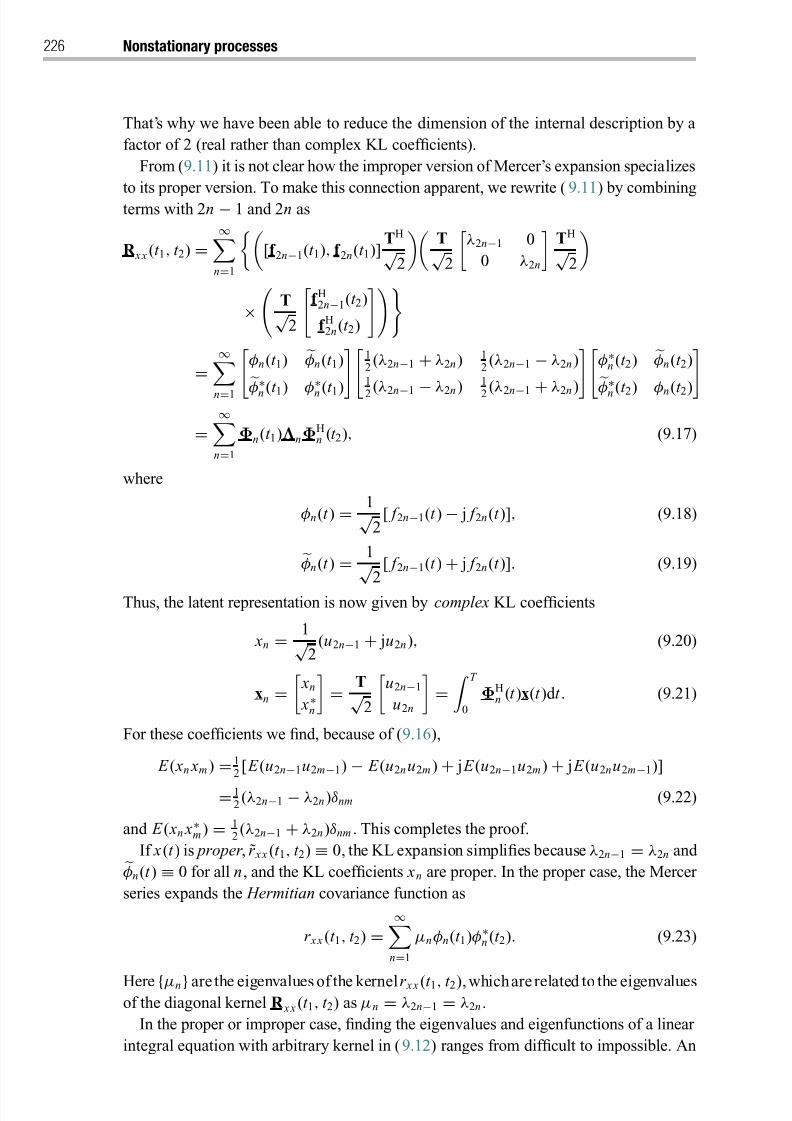
8/21/2019 Statistical Signal Processing of Complex-Valued Data.pdf
http://slidepdf.com/reader/full/statistical-signal-processing-of-complex-valued-datapdf 248/330
226 Nonstationary processes
That’s why we have been able to reduce the dimension of the internal description by a
factor of 2 (real rather than complex KL coefficients).
From (9.11) it is not clear how the improper version of Mercer’s expansion specializes
to its proper version. To make this connection apparent, we rewrite (9.11) by combining
terms with 2n − 1 and 2n as
R x x (t 1, t 2) =∞
n=1
[f 2n−1(t 1), f 2n(t 1)]
TH
√ 2
T√
2
λ2n−1 0
0 λ2n
TH
√ 2
×
T√ 2
f H2n−1(t 2)
f H2n(t 2)
=
∞
n=1 φn(t 1)
φn(t 1)
φ∗n (t 1) φ∗n (t 1)12(λ2n−1 + λ2n) 1
2(λ2n−1 − λ2n)
1
2 (λ2n−1 − λ2n)
1
2 (λ2n−1 + λ2n)φ∗
n (t 2)
φn(t 2)
φ∗n (t 2) φn(t 2)=
∞n=1
Φn(t 1)ΛnΦHn (t 2), (9.17)
where
φn(t ) = 1√ 2
[ f 2n−1(t ) − j f 2n(t )], (9.18)
φn(t ) = 1√
2[ f 2n−1(t ) + j f 2n(t )]. (9.19)
Thus, the latent representation is now given by complex KL coefficients
xn =1√ 2
(u2n−1 + ju2n), (9.20)
xn =
xn
x∗n
= T√
2
u2n−1
u2n
= T
0
ΦHn (t )x(t )d t . (9.21)
For these coefficients we find, because of (9.16),
E ( xn xm)
=12[ E (u2n−1u2m−1)
− E (u2n u2m)
+ j E (u2n−1u2m)
+ j E (u2nu2m−1)]
= 12(λ2n−1 − λ2n)δnm (9.22)
and E ( xn x∗m) = 12(λ2n−1 + λ2n)δnm . This completes the proof.
If x (t ) is proper , r x x (t 1, t 2) ≡ 0, the KL expansion simplifies because λ2n−1 = λ2n and φn(t ) ≡ 0 for all n, and the KL coefficients xn are proper. In the proper case, the Mercer
series expands the Hermitian covariance function as
r x x (t 1, t 2) =∞
n=1
µn φn(t 1)φ∗n (t 2). (9.23)
Here {µn} are the eigenvalues of the kernelr x x (t 1, t 2), whicharerelated to the eigenvaluesof the diagonal kernel R x x (t 1, t 2) as µn = λ2n−1 = λ2n .
In the proper or improper case, finding the eigenvalues and eigenfunctions of a linear
integral equation with arbitrary kernel in (9.12) ranges from difficult to impossible. An
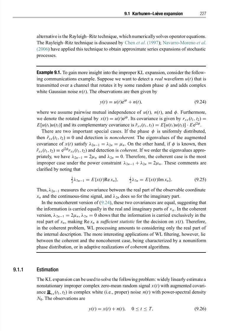
8/21/2019 Statistical Signal Processing of Complex-Valued Data.pdf
http://slidepdf.com/reader/full/statistical-signal-processing-of-complex-valued-datapdf 249/330
9.1 Karhunen–Lo eve expansion 227
alternative is the Rayleigh–Ritz technique, which numerically solves operator equations.
The Rayleigh–Ritz technique is discussed by Chen et al . (1997); Navarro-Moreno et al .
(2006) have applied this technique to obtain approximate series expansions of stochastic
processes.
Example 9.1. To gain more insight into the improper KL expansion, consider the follow-
ing communications example. Suppose we want to detect a real waveform u(t ) that is
transmitted over a channel that rotates it by some random phase φ and adds complex
white Gaussian noise n(t ). The observations are then given by
y(t ) = u(t )e jφ + n(t ), (9.24)
where we assume pairwise mutual independence of u(t ), n(t ), and φ. Furthermore,
we denote the rotated signal by x(t ) = u(t )e jφ . Its covariance is given by r x x (t 1, t 2) = E [u(t 1)u(t 2)] and its complementary covariance is r x x (t 1, t 2) = E [u(t 1)u(t 2)] · E e j2φ .
There are two important special cases. If the phase φ is uniformly distributed,
then r x x (t 1, t 2) ≡ 0 and detection is noncoherent . The eigenvalues of the augmented
covariance of x(t ) satisfy λ2n−1 = λ2n = µn . On the other hand, if φ is known, then
r x x (t 1, t 2) ≡ e j2φr x x (t 1, t 2) and detection is coherent . If we order the eigenvalues appro-
priately, we have λ2n−1 = 2µn and λ2n = 0. Therefore, the coherent case is the most
improper case under the power constraint λ2n−1 + λ2n = 2µn . These comments are
clarified by noting that
12
λ2n−1 = E { x(t )Re xn}, j
2λ2n = E { x(t )Im xn}. (9.25)
Thus, λ2n−1 measures the covariance between the real part of the observable coordinate
xn and the continuous-time signal, and λ2n does so for the imaginary part.
In the noncoherent version of (9.24), these two covariances are equal, suggesting that
the information is carried equally in the real and imaginary parts of x n . In the coherent
version, λ2n−1 = 2µn , λ2n = 0 shows that the information is carried exclusively in the
real part of xn , making Re xn a sufficient statistic for the decision on x(t ). Therefore,
in the coherent problem, WL processing amounts to considering only the real part of
the internal description. The more interesting applications of WL filtering, however, lie
between the coherent and the noncoherent case, being characterized by a nonuniform
phase distribution, or in adaptive realizations of coherent algorithms.
9.1.1 Estimation
The KL expansion can be used to solve the following problem: widely linearly estimate a
nonstationary improper complex zero-mean random signal x (t ) with augmented covari-
ance R x x (t 1, t 2) in complex white (i.e., proper) noise n(t ) with power-spectral density
N 0. The observations are
y(t ) = x(t ) + n(t ), 0 ≤ t ≤ T , (9.26)
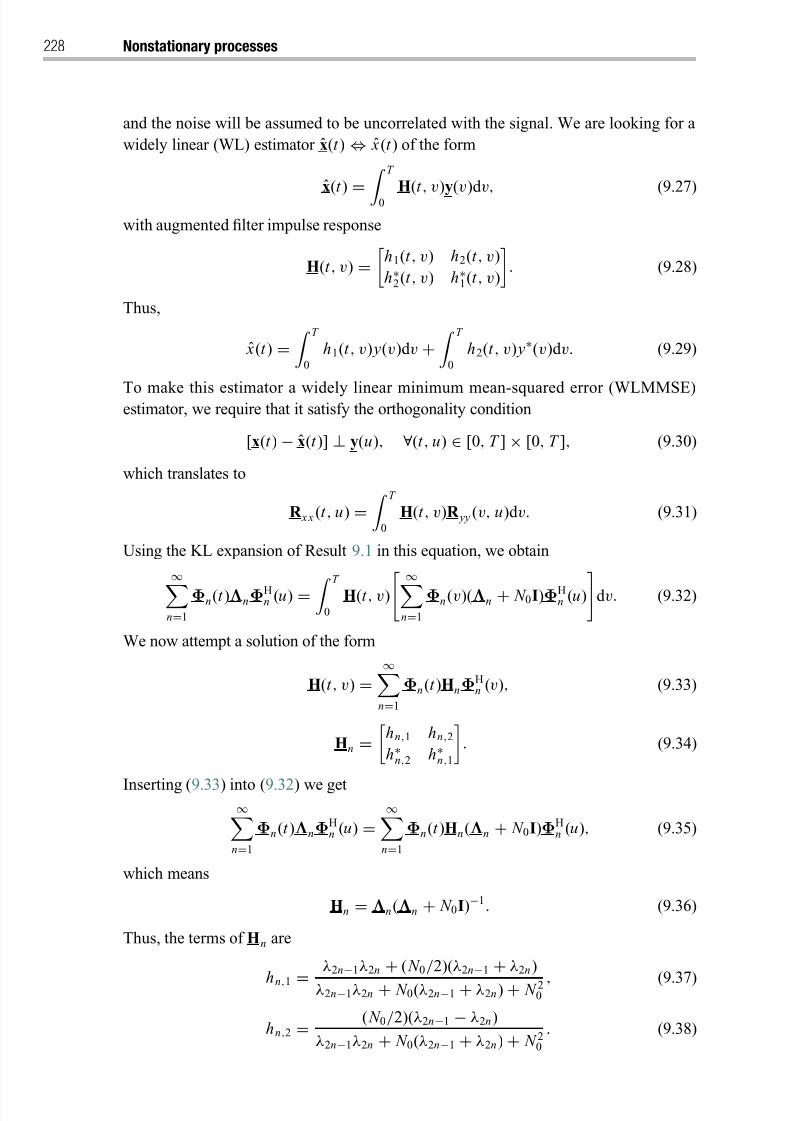
8/21/2019 Statistical Signal Processing of Complex-Valued Data.pdf
http://slidepdf.com/reader/full/statistical-signal-processing-of-complex-valued-datapdf 250/330
228 Nonstationary processes
and the noise will be assumed to be uncorrelated with the signal. We are looking for a
widely linear (WL) estimator x(t ) ⇔ ˆ x(t ) of the form
x(t )=
T
0
H(t , v)y(v)d v, (9.27)
with augmented filter impulse response
H(t , v) =
h1(t , v) h2(t , v)
h∗2(t , v) h∗
1(t , v)
. (9.28)
Thus,
ˆ x(t ) = T
0
h1(t , v) y(v)d v + T
0
h2(t , v) y∗(v)d v. (9.29)
To make this estimator a widely linear minimum mean-squared error (WLMMSE)estimator, we require that it satisfy the orthogonality condition
[x(t ) − x(t )] ⊥ y(u), ∀(t , u) ∈ [0, T ] × [0, T ], (9.30)
which translates to
R x x (t , u) = T
0
H(t , v)R yy (v, u)d v. (9.31)
Using the KL expansion of Result 9.1 in this equation, we obtain
∞n=1
Φn(t )ΛnΦHn (u) = T
0
H(t , v) ∞n=1
Φn(v)(Λn + N 0I)ΦHn (u)d v. (9.32)
We now attempt a solution of the form
H(t , v) =∞
n=1
Φn(t )HnΦHn (v), (9.33)
Hn =
hn,1 hn,2
h∗n,2 h∗
n,1
. (9.34)
Inserting (9.33) into (9.32) we get∞
n=1
Φn(t )ΛnΦHn (u) =
∞n=1
Φn(t )Hn(Λn + N 0I)ΦHn (u), (9.35)
which means
Hn = Λn(Λn + N 0I)−1. (9.36)
Thus, the terms of Hn are
hn,1 =λ2n
−1λ2n
+( N 0/2)(λ2n
−1
+λ2n)
λ2n−1λ2n + N 0(λ2n−1 + λ2n) + N 20 , (9.37)
hn,2 =( N 0/2)(λ2n−1 − λ2n)
λ2n−1λ2n + N 0(λ2n−1 + λ2n) + N 20. (9.38)
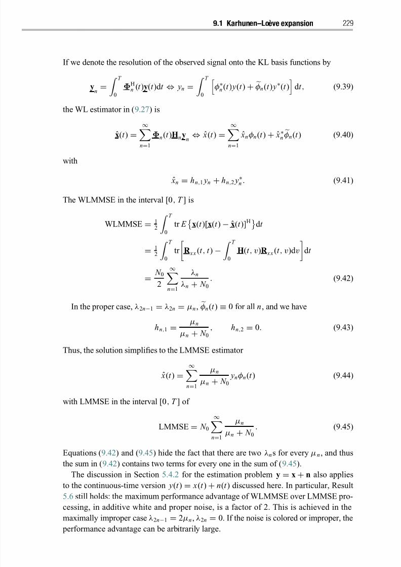
8/21/2019 Statistical Signal Processing of Complex-Valued Data.pdf
http://slidepdf.com/reader/full/statistical-signal-processing-of-complex-valued-datapdf 251/330
9.1 Karhunen–Lo eve expansion 229
If we denote the resolution of the observed signal onto the KL basis functions by
yn =
T
0
ΦHn (t )y(t )d t ⇔ yn =
T
0 φ∗
n (t ) y(t ) + φn(t ) y∗(t )
d t , (9.39)
the WL estimator in (9.27) is
x(t ) =∞
n=1
Φn(t )Hn yn ⇔ ˆ x(t ) =
∞n=1
ˆ xn φn(t ) + ˆ x∗n φn(t ) (9.40)
with
ˆ xn = hn,1 yn + hn,2 y∗n . (9.41)
The WLMMSE in the interval [0, T ] is
WLMMSE = 12
T
0
tr E
x(t )[x(t ) − x(t )]H
d t
= 12
T
0
tr
R x x (t , t ) −
T
0
H(t , v)R x x (t , v)d v
d t
= N 0
2
∞n=1
λn
λn + N 0. (9.42)
In the proper case, λ2n−1 = λ2n = µn , φn(t ) ≡ 0 for all n , and we have
hn,1 =µn
µn + N 0, hn,2 = 0. (9.43)
Thus, the solution simplifies to the LMMSE estimator
ˆ x(t ) =∞
n=1
µn
µn + N 0 ynφn(t ) (9.44)
with LMMSE in the interval [0, T ] of
LMMSE = N 0
∞n=1
µn
µn + N 0. (9.45)
Equations (9.42) and (9.45) hide the fact that there are two λns for every µn , and thus
the sum in (9.42) contains two terms for every one in the sum of (9.45).
The discussion in Section 5.4.2 for the estimation problem y = x + n also applies
to the continuous-time version y(t ) = x(t ) + n(t ) discussed here. In particular, Result
5.6 still holds: the maximum performance advantage of WLMMSE over LMMSE pro-cessing, in additive white and proper noise, is a factor of 2. This is achieved in the
maximally improper case λ2n−1 = 2µn , λ2n = 0. If the noise is colored or improper, the
performance advantage can be arbitrarily large.
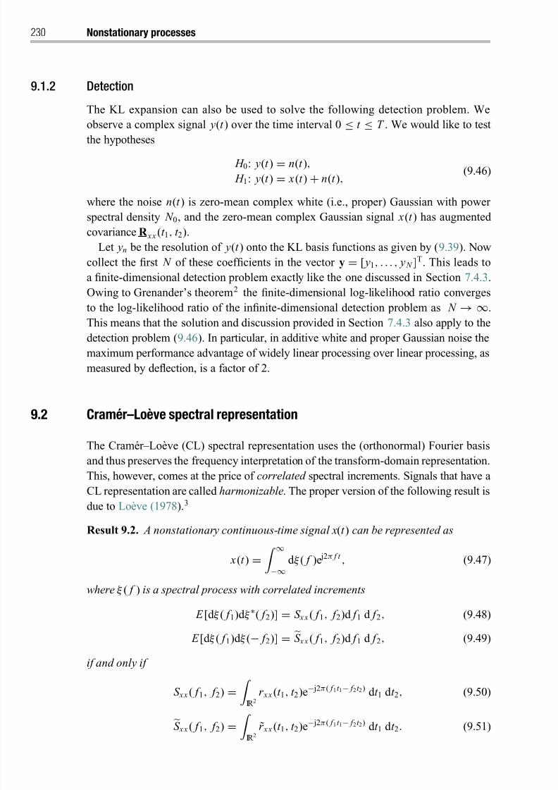
8/21/2019 Statistical Signal Processing of Complex-Valued Data.pdf
http://slidepdf.com/reader/full/statistical-signal-processing-of-complex-valued-datapdf 252/330
230 Nonstationary processes
9.1.2 Detection
The KL expansion can also be used to solve the following detection problem. We
observe a complex signal y(t ) over the time interval 0
≤t
≤T . We would like to test
the hypotheses
H 0: y(t ) = n(t ),
H 1: y(t ) = x(t ) + n(t ), (9.46)
where the noise n(t ) is zero-mean complex white (i.e., proper) Gaussian with power
spectral density N 0, and the zero-mean complex Gaussian signal x(t ) has augmented
covariance R x x (t 1, t 2).
Let yn be the resolution of y(t ) onto the KL basis functions as given by (9.39). Now
collect the first N of these coefficients in the vector y
=[ y1, . . . , y N ]
T. This leads to
a finite-dimensional detection problem exactly like the one discussed in Section 7.4.3.Owing to Grenander’s theorem2 the finite-dimensional log-likelihood ratio converges
to the log-likelihood ratio of the infinite-dimensional detection problem as N → ∞.
This means that the solution and discussion provided in Section 7.4.3 also apply to the
detection problem (9.46). In particular, in additive white and proper Gaussian noise the
maximum performance advantage of widely linear processing over linear processing, as
measured by deflection, is a factor of 2.
9.2 Cram ´ er–Lo eve spectral representation
The Cramer–Loeve (CL) spectral representation uses the (orthonormal) Fourier basis
and thus preserves the frequency interpretation of the transform-domain representation.
This, however, comes at the price of correlated spectral increments. Signals that have a
CL representation are called harmonizable. The proper version of the following result is
due to Loeve (1978).3
Result 9.2. A nonstationary continuous-time signal x(t ) can be represented as
x(t ) = ∞−∞
d ξ ( f )e j2π f t , (9.47)
where ξ ( f ) is a spectral process with correlated increments
E [d ξ ( f 1)d ξ ∗( f 2)] = S x x ( f 1, f 2)d f 1 d f 2, (9.48)
E [d ξ ( f 1)d ξ (− f 2)] = S x x ( f 1, f 2)d f 1 d f 2, (9.49)
if and only if
S x x ( f 1, f 2) = IR 2
r x x (t 1, t 2)e− j2π( f 1t 1− f 2t 2) d t 1 d t 2, (9.50)
S x x ( f 1, f 2) =
IR 2r x x (t 1, t 2)e− j2π( f 1t 1− f 2t 2) d t 1 d t 2. (9.51)
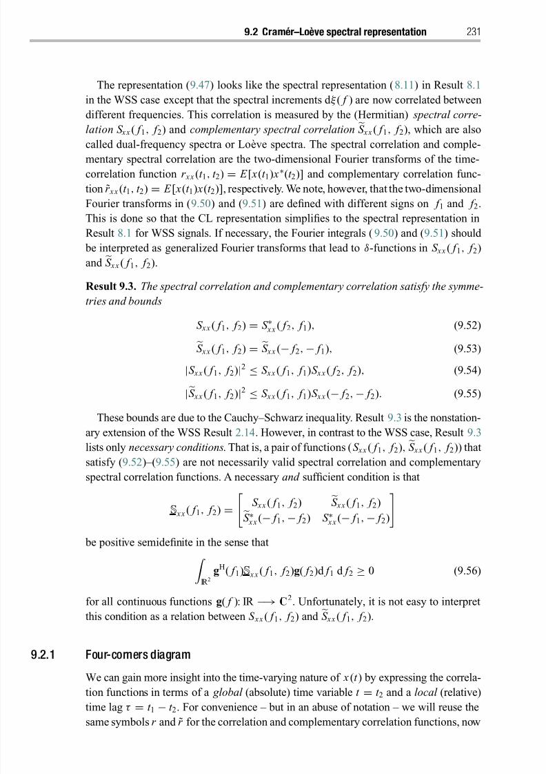
8/21/2019 Statistical Signal Processing of Complex-Valued Data.pdf
http://slidepdf.com/reader/full/statistical-signal-processing-of-complex-valued-datapdf 253/330
9.2 Cram ´ er–Lo eve spectral representation 231
The representation (9.47) looks like the spectral representation (8.11) in Result 8.1
in the WSS case except that the spectral increments d ξ ( f ) are now correlated between
different frequencies. This correlation is measured by the (Hermitian) spectral corre-
lation S x x
( f 1
, f 2) and complementary spectral correlation S
x x( f
1, f
2), which are also
called dual-frequency spectra or Loeve spectra. The spectral correlation and comple-
mentary spectral correlation are the two-dimensional Fourier transforms of the time-
correlation function r x x (t 1, t 2) = E [ x(t 1) x∗(t 2)] and complementary correlation func-
tion r x x (t 1, t 2) = E [ x(t 1) x(t 2)], respectively. We note, however, that the two-dimensional
Fourier transforms in (9.50) and (9.51) are defined with different signs on f 1 and f 2.
This is done so that the CL representation simplifies to the spectral representation in
Result 8.1 for WSS signals. If necessary, the Fourier integrals (9.50) and (9.51) should
be interpreted as generalized Fourier transforms that lead to δ-functions in S x x ( f 1, f 2)
and S x x ( f 1, f 2).
Result 9.3. The spectral correlation and complementary correlation satisfy the symme-
tries and bounds
S x x ( f 1, f 2) = S ∗ x x ( f 2, f 1), (9.52)S x x ( f 1, f 2) = S x x (− f 2,− f 1), (9.53)
|S x x ( f 1, f 2)|2 ≤ S x x ( f 1, f 1)S x x ( f 2, f 2), (9.54)
|S x x ( f 1, f 2)
|2
≤ S x x ( f 1, f 1)S x x (
− f 2,
− f 2). (9.55)
These bounds are due to the Cauchy–Schwarz inequality. Result 9.3 is the nonstation-
ary extension of the WSS Result 2.14. However, in contrast to the WSS case, Result 9.3
lists only necessary conditions. That is, a pair of functions (S x x ( f 1, f 2), S x x ( f 1, f 2)) that
satisfy (9.52)–(9.55) are not necessarily valid spectral correlation and complementary
spectral correlation functions. A necessary and sufficient condition is that
S x x ( f 1, f 2) =
S x x ( f 1, f 2) S x x ( f 1, f 2)
S ∗ x x (− f 1,− f 2) S ∗ x x (− f 1,− f 2)
be positive semidefinite in the sense that IR 2
gH( f 1)S x x ( f 1, f 2)g( f 2)d f 1 d f 2 ≥ 0 (9.56)
for all continuous functions g( f ): IR −→ C2. Unfortunately, it is not easy to interpret
this condition as a relation between S x x ( f 1, f 2) and S x x ( f 1, f 2).
9.2.1 Four-corners diagram
We can gain more insight into the time-varying nature of x (t ) by expressing the correla-tion functions in terms of a global (absolute) time variable t = t 2 and a local (relative)
time lag τ = t 1 − t 2. For convenience – but in an abuse of notation – we will reuse the
same symbols r and r for the correlation and complementary correlation functions, now
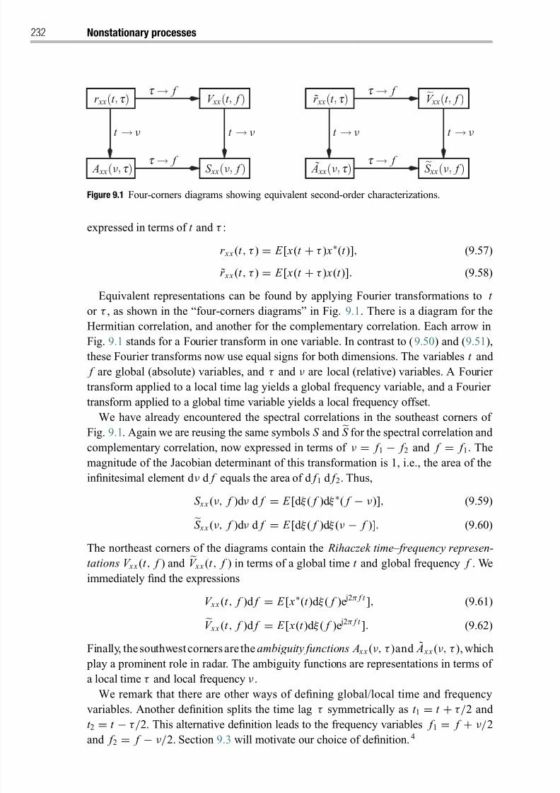
8/21/2019 Statistical Signal Processing of Complex-Valued Data.pdf
http://slidepdf.com/reader/full/statistical-signal-processing-of-complex-valued-datapdf 254/330
232 Nonstationary processes
t → f
V xx(t f )
S xx(ν f )S xx(ν f ) ˜ A xx(ν t )
r xx(t t )V xx(t f )
A xx(ν t )
r xx(t t )
t → f
t →
νt →
ν
t → f t → f
t →
ν t →
ν
Figure 9.1 Four-corners diagrams showing equivalent second-order characterizations.
expressed in terms of t and τ :
r x x (t , τ ) = E [ x(t + τ ) x∗(t )], (9.57)
r x x (t , τ ) = E [ x(t + τ ) x(t )]. (9.58)Equivalent representations can be found by applying Fourier transformations to t
or τ , as shown in the “four-corners diagrams” in Fig. 9.1. There is a diagram for the
Hermitian correlation, and another for the complementary correlation. Each arrow in
Fig. 9.1 stands for a Fourier transform in one variable. In contrast to (9.50) and (9.51),
these Fourier transforms now use equal signs for both dimensions. The variables t and
f are global (absolute) variables, and τ and ν are local (relative) variables. A Fourier
transform applied to a local time lag yields a global frequency variable, and a Fourier
transform applied to a global time variable yields a local frequency offset.
We have already encountered the spectral correlations in the southeast corners of Fig. 9.1. Again we are reusing the same symbols S and S for the spectral correlation and
complementary correlation, now expressed in terms of ν = f 1 − f 2 and f = f 1. The
magnitude of the Jacobian determinant of this transformation is 1, i.e., the area of the
infinitesimal element d ν d f equals the area of d f 1 d f 2. Thus,
S x x (ν, f )d ν d f = E [d ξ ( f )d ξ ∗( f − ν)], (9.59)
S x x (ν, f )d ν d f = E [d ξ ( f )d ξ (ν − f )]. (9.60)
The northeast corners of the diagrams contain the Rihaczek time–frequency represen-
tations V x x (t , f ) and V x x (t , f ) in terms of a global time t and global frequency f . We
immediately find the expressions
V x x (t , f )d f = E [ x∗(t )d ξ ( f )e j2π f t ], (9.61)V x x (t , f )d f = E [ x(t )d ξ ( f )e j2π f t ]. (9.62)
Finally, thesouthwestcornersare the ambiguity functions A x x (ν, τ )and ˜ A x x (ν, τ ), which
play a prominent role in radar. The ambiguity functions are representations in terms of
a local time τ and local frequency ν .
We remark that there are other ways of defining global/local time and frequencyvariables. Another definition splits the time lag τ symmetrically as t 1 = t + τ/2 and
t 2 = t − τ/2. This alternative definition leads to the frequency variables f 1 = f + ν/2
and f 2 = f − ν/2. Section 9.3 will motivate our choice of definition.4
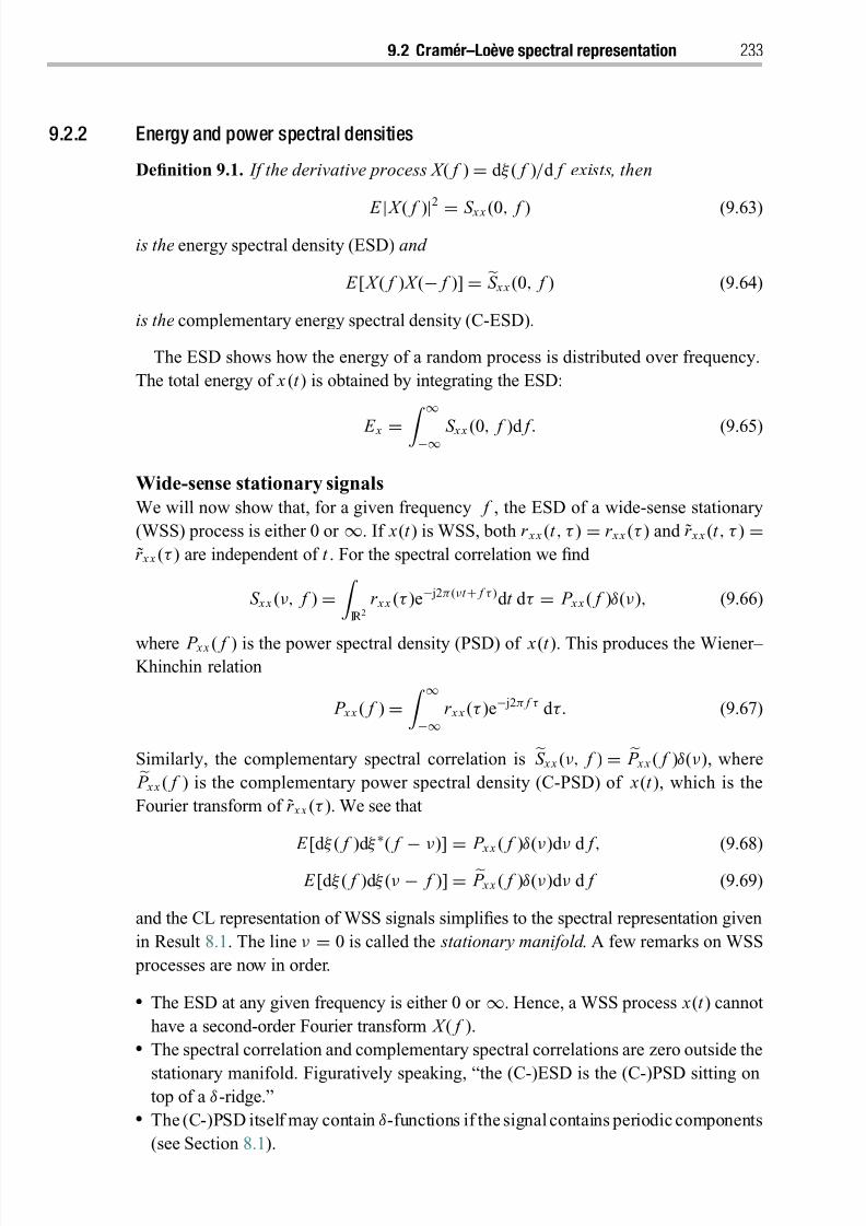
8/21/2019 Statistical Signal Processing of Complex-Valued Data.pdf
http://slidepdf.com/reader/full/statistical-signal-processing-of-complex-valued-datapdf 255/330
9.2 Cram ´ er–Lo eve spectral representation 233
9.2.2 Energy and power spectral densities
Definition 9.1. If the derivative process X ( f ) = d ξ ( f )/d f exists, then
E | X ( f )|2
= S x x (0, f ) (9.63)
is the energy spectral density (ESD) and
E [ X ( f ) X (− f )] = S x x (0, f ) (9.64)
is the complementary energy spectral density (C-ESD).
The ESD shows how the energy of a random process is distributed over frequency.
The total energy of x (t ) is obtained by integrating the ESD:
E x = ∞−∞ S x x (0, f )d f . (9.65)
Wide-sense stationary signals
We will now show that, for a given frequency f , the ESD of a wide-sense stationary
(WSS) process is either 0 or ∞. If x(t ) is WSS, both r x x (t , τ ) = r x x (τ ) and r x x (t , τ ) =r x x (τ ) are independent of t . For the spectral correlation we find
S x x (ν, f ) =
IR 2r x x (τ )e− j2π(νt + f τ )d t d τ = P x x ( f )δ(ν), (9.66)
where P x x ( f ) is the power spectral density (PSD) of x(t ). This produces the Wiener– Khinchin relation
P x x ( f ) = ∞−∞
r x x (τ )e− j2π f τ d τ. (9.67)
Similarly, the complementary spectral correlation is S x x (ν, f ) = P x x ( f )δ(ν), where P x x ( f ) is the complementary power spectral density (C-PSD) of x(t ), which is the
Fourier transform of r x x (τ ). We see that
E [d ξ ( f )d ξ ∗( f
−ν)]
= P x x ( f )δ(ν)d ν d f , (9.68)
E [d ξ ( f )d ξ (ν − f )] = P x x ( f )δ(ν)d ν d f (9.69)
and the CL representation of WSS signals simplifies to the spectral representation given
in Result 8.1. The line ν = 0 is called the stationary manifold . A few remarks on WSS
processes are now in order.
The ESD at any given frequency is either 0 or ∞. Hence, a WSS process x(t ) cannot
have a second-order Fourier transform X ( f ). The spectral correlation and complementary spectral correlations are zero outside the
stationary manifold. Figuratively speaking, “the (C-)ESD is the (C-)PSD sitting ontop of a δ-ridge.”
The (C-)PSD itself may contain δ-functions if thesignal contains periodic components
(see Section 8.1).
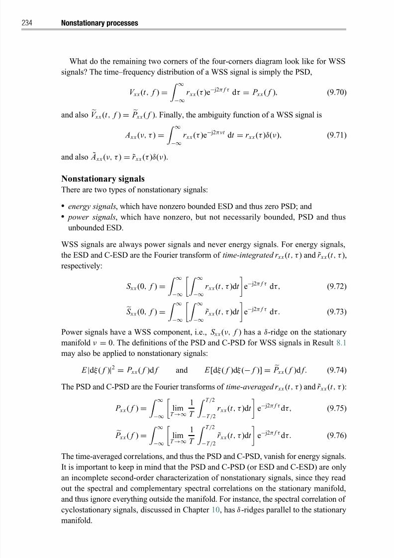
8/21/2019 Statistical Signal Processing of Complex-Valued Data.pdf
http://slidepdf.com/reader/full/statistical-signal-processing-of-complex-valued-datapdf 256/330
234 Nonstationary processes
What do the remaining two corners of the four-corners diagram look like for WSS
signals? The time–frequency distribution of a WSS signal is simply the PSD,
V x x (t , f )=
∞
−∞r x x (τ )e− j2π f τ d τ
= P x x ( f ), (9.70)
and also V x x (t , f ) = P x x ( f ). Finally, the ambiguity function of a WSS signal is
A x x (ν, τ ) = ∞−∞
r x x (τ )e− j2π νt d t = r x x (τ )δ(ν), (9.71)
and also ˜ A x x (ν, τ ) = r x x (τ )δ(ν).
Nonstationary signals
There are two types of nonstationary signals:
energy signals, which have nonzero bounded ESD and thus zero PSD; and power signals, which have nonzero, but not necessarily bounded, PSD and thus
unbounded ESD.
WSS signals are always power signals and never energy signals. For energy signals,
the ESD and C-ESD are the Fourier transform of time-integrated r x x (t , τ ) and r x x (t , τ ),
respectively:
S x x (0, f )
= ∞
−∞ ∞
−∞r x x (t , τ )d t e− j2π f τ d τ, (9.72)
S x x (0, f ) = ∞−∞
∞−∞
r x x (t , τ )d t
e− j2π f τ d τ. (9.73)
Power signals have a WSS component, i.e., S x x (ν, f ) has a δ-ridge on the stationary
manifold ν = 0. The definitions of the PSD and C-PSD for WSS signals in Result 8.1
may also be applied to nonstationary signals:
E |d ξ ( f )|2 = P x x ( f )d f and E [d ξ ( f )d ξ (− f )] =
P x x ( f )d f . (9.74)
The PSD and C-PSD are the Fourier transforms of time-averaged r x x
(t , τ ) and r x x
(t , τ ):
P x x ( f ) = ∞−∞
limT →∞
1
T
T /2
−T /2
r x x (t , τ )d t
e− j2π f τ d τ, (9.75)
P x x ( f ) = ∞−∞
limT →∞
1
T
T /2
−T /2
r x x (t , τ )d t
e− j2π f τ d τ. (9.76)
The time-averaged correlations, and thus the PSD and C-PSD, vanish for energy signals.
It is important to keep in mind that the PSD and C-PSD (or ESD and C-ESD) are only
an incomplete second-order characterization of nonstationary signals, since they read
out the spectral and complementary spectral correlations on the stationary manifold,and thus ignore everything outside the manifold. For instance, the spectral correlation of
cyclostationary signals, discussed in Chapter 10, has δ-ridges parallel to the stationary
manifold.
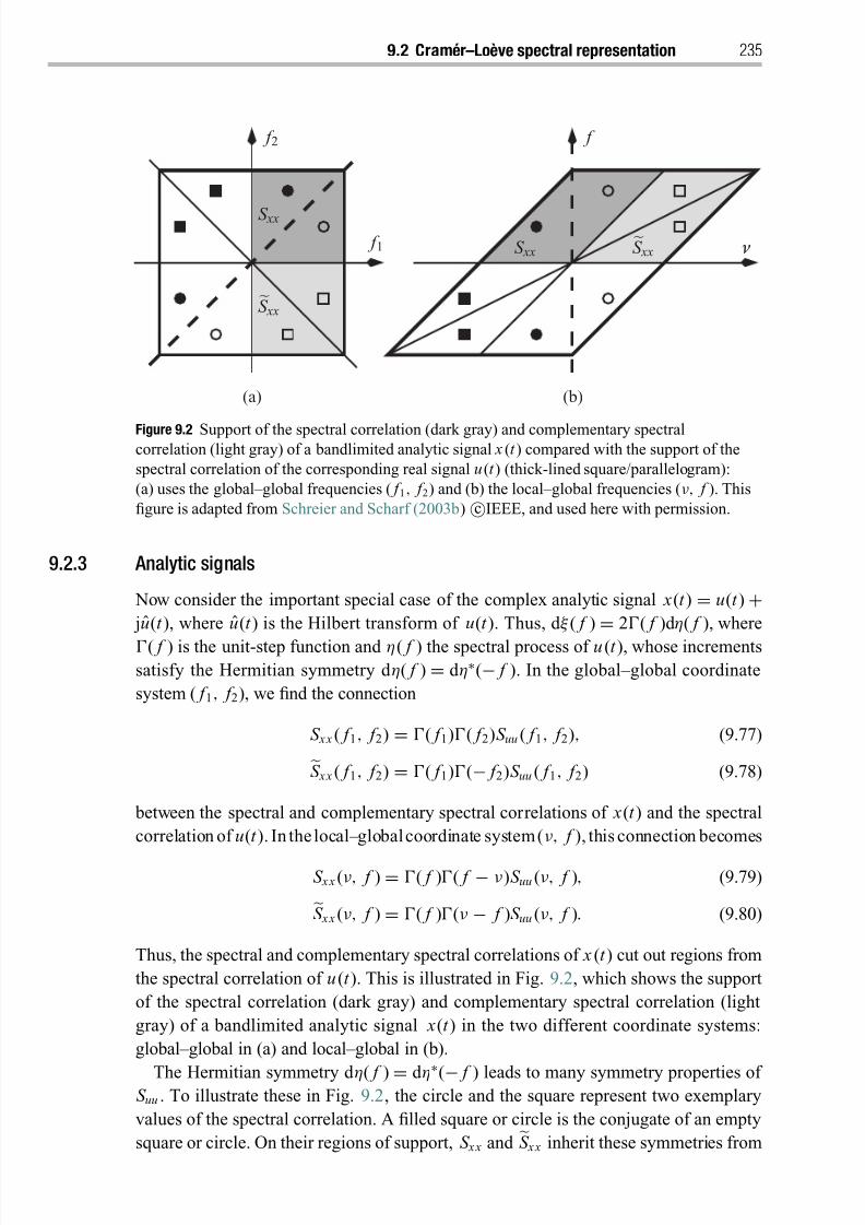
8/21/2019 Statistical Signal Processing of Complex-Valued Data.pdf
http://slidepdf.com/reader/full/statistical-signal-processing-of-complex-valued-datapdf 257/330
9.2 Cram ´ er–Lo eve spectral representation 235
(a) (b)
S xxS xx
S xx
S xx
f 2
f 1
f
ν
Figure 9.2 Support of the spectral correlation (dark gray) and complementary spectralcorrelation (light gray) of a bandlimited analytic signal x (t ) compared with the support of the
spectral correlation of the corresponding real signal u(t ) (thick-lined square/parallelogram):
(a) uses the global–global frequencies ( f 1, f 2) and (b) the local–global frequencies (ν, f ). This
figure is adapted from Schreier and Scharf (2003b) cIEEE, and used here with permission.
9.2.3 Analytic signals
Now consider the important special case of the complex analytic signal x(t ) = u(t ) + ju(t ), where u(t ) is the Hilbert transform of u(t ). Thus, d ξ ( f )
=2( f )d η( f ), where
( f ) is the unit-step function and η( f ) the spectral process of u (t ), whose incrementssatisfy the Hermitian symmetry d η( f ) = d η∗(− f ). In the global–global coordinate
system ( f 1, f 2), we find the connection
S x x ( f 1, f 2) = ( f 1)( f 2)S uu ( f 1, f 2), (9.77)S x x ( f 1, f 2) = ( f 1)(− f 2)S uu ( f 1, f 2) (9.78)
between the spectral and complementary spectral correlations of x(t ) and the spectral
correlation of u(t ). In thelocal–globalcoordinate system(ν, f ), this connection becomes
S x x (ν, f ) = ( f )( f − ν)S uu (ν, f ), (9.79)S x x (ν, f ) = ( f )(ν − f )S uu (ν, f ). (9.80)
Thus, the spectral and complementary spectral correlations of x (t ) cut out regions from
the spectral correlation of u(t ). This is illustrated in Fig. 9.2, which shows the support
of the spectral correlation (dark gray) and complementary spectral correlation (light
gray) of a bandlimited analytic signal x(t ) in the two different coordinate systems:
global–global in (a) and local–global in (b).
The Hermitian symmetry d η( f ) = d η∗(− f ) leads to many symmetry properties of S uu . To illustrate these in Fig. 9.2, the circle and the square represent two exemplary
values of the spectral correlation. A filled square or circle is the conjugate of an empty
square or circle. On their regions of support, S x x and S x x inherit these symmetries from
8/21/2019 Statistical Signal Processing of Complex-Valued Data.pdf
http://slidepdf.com/reader/full/statistical-signal-processing-of-complex-valued-datapdf 258/330
236 Nonstationary processes
ν
f
f s
f s
Figure 9.3 Aliasing in the spectral correlation of x [k ].
S uu . Figure 9.2 also shows how S x x complements the information in S x x . It is clearly not
possible to reconstruct S uu from S x x alone.
The stationary manifold is the dashed line in Fig. 9.2. This line does not pass through
the region of support of S x x . This proves once again that WSS analytic signals – whose
support is limited to the stationary manifold – must be proper.
9.2.4 Discrete-time signals
We now investigate what happens if we sample the random process x(t ) with sampling
frequency f s = T −1s to obtain x [k ] = x(kT s). The spectral representation of the sampled
process x [k ] is
x[k ] = ∞−∞
e j2π f k T s d ξ ( f )
= f s/2
− f s/2 e j 2π
f s
f k ∞
m=−∞ d ξ ( f + m f s). (9.81)
The spectral representation of x[k ] is thus subject to aliasing unless d ξ ( f ) = 0 for
| f | > f s/2. The spectral correlation of x [k ] is
S d x x (ν, f ) =
∞m=−∞
∞n=−∞
S x x (ν + m f s, f + n f s), (9.82)
where the letter d stands for discrete-time. The same formula is obtained for the com-
plementary spectral correlation. The term with m = 0 and n = 0 in (9.82) is called the
principal replica of S x x (ν, f ). Figure 9.3 illustrates aliasing for the spectral correla-tion of a bandlimited, undersampled, signal. The support of the principal replica is the
thick-lined parallelogram centered at the origin. Figure 9.3 also shows the replicas that
8/21/2019 Statistical Signal Processing of Complex-Valued Data.pdf
http://slidepdf.com/reader/full/statistical-signal-processing-of-complex-valued-datapdf 259/330
9.3 Rihaczek time–frequency representation 237
overlap with the principal replica. Areas of overlap are gray. The following points are
noteworthy.
There are regions of the principal replica that overlap with one other replica (light
gray) and regions that overlap with three other replicas (dark gray). (This assumes, asin Fig. 9.3, that d ξ ( f ) = 0 for | f | > f s; otherwise the principal replica could overlap
with further replicas.) In general, replicas with m = 0 and/or n = 0 contribute to aliasing in the ESD or PSD
along the stationary manifold ν = 0. However, the spectral correlation of a WSS signal is zero off the stationary manifold.
Therefore, only the replicas with m = 0 and n = 0 can contribute to aliasing in the
PSD of a WSS signal.
9.3 Rihaczek time–frequency representation
Let’s explore some of the properties of the Rihaczek time–frequency representa-
tion,5 which is comprised of the Hermitian Rihaczek time–frequency distribution
(HR-TFD)
V x x (t , f ) = ∞−∞
r x x (t , τ )e− j2π f τ d τ (9.83)
and the complementary Rihaczek time–frequency distribution (CR-TFD)
V x x (t , f ) = ∞−∞
r x x (t , τ )e− j2π f τ d τ. (9.84)
It is obvious that the Rihaczek time–frequency representation is shift-covariant in both
time and frequency:
x(t − t 0) ←→ V x x (t − t 0, f ), V x x (t − t 0, f ), (9.85)
x(t )e j2π f 0t
←→ V x x (t , f
− f 0), V x x (t , f
− f 0). (9.86)
Both the HR-TFD and CR-TFD are generally complex-valued. However, the time-
marginal of the HR-TFD ∞−∞
V x x (t , f )d f = r x x (t , 0) = E | x(t )|2 ≥ 0, (9.87)
which is the instantaneous power at t , and the frequency-marginal of the HR-TFD ∞−∞
V x x (t , f )d t = S x x (0, f ) ≥ 0, (9.88)
which is the energy spectral density at f , are nonnegative.It is common to interpret time–frequency distributions as distributions of energy
or power over time and frequency. However, such an interpretation is fraught with
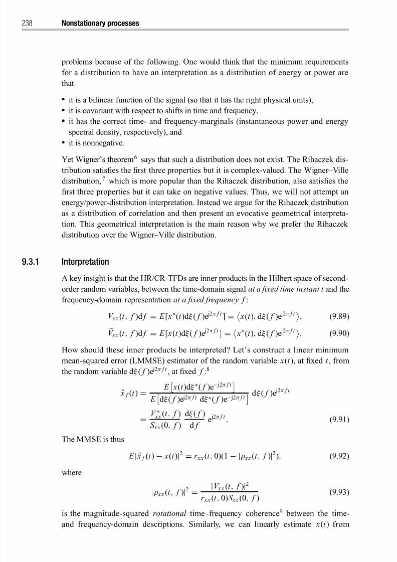
8/21/2019 Statistical Signal Processing of Complex-Valued Data.pdf
http://slidepdf.com/reader/full/statistical-signal-processing-of-complex-valued-datapdf 260/330
238 Nonstationary processes
problems because of the following. One would think that the minimum requirements
for a distribution to have an interpretation as a distribution of energy or power are
that
it is a bilinear function of the signal (so that it has the right physical units), it is covariant with respect to shifts in time and frequency, it has the correct time- and frequency-marginals (instantaneous power and energy
spectral density, respectively), and it is nonnegative.
Yet Wigner’s theorem6 says that such a distribution does not exist. The Rihaczek dis-
tribution satisfies the first three properties but it is complex-valued. The Wigner–Ville
distribution,7 which is more popular than the Rihaczek distribution, also satisfies the
first three properties but it can take on negative values. Thus, we will not attempt an
energy/power-distribution interpretation. Instead we argue for the Rihaczek distribution
as a distribution of correlation and then present an evocative geometrical interpreta-
tion. This geometrical interpretation is the main reason why we prefer the Rihaczek
distribution over the Wigner–Ville distribution.
9.3.1 Interpretation
A key insight is that the HR/CR-TFDs are inner products in the Hilbert space of second-
order random variables, between the time-domain signal at a fixed time instant t and the
frequency-domain representation at a fixed frequency f :
V x x (t , f )d f = E [ x∗(t )d ξ ( f )e j2π f t ] = x(t ), d ξ ( f )e j2π f t
, (9.89)V x x (t , f )d f = E [ x(t )d ξ ( f )e j2π f t ] = x∗(t ), d ξ ( f )e j2π f t
. (9.90)
How should these inner products be interpreted? Let’s construct a linear minimum
mean-squared error (LMMSE) estimator of the random variable x(t ), at fixed t , from
the random variable d ξ ( f )e j2π f t , at fixed f :8
ˆ x f (t ) = E x(t )d ξ ∗( f )e− j2π f t E d ξ ( f )e j2π f t d ξ ∗( f )e− j2π f t d ξ ( f )e
j2π f t
= V ∗ x x (t , f )
S x x (0, f )
d ξ ( f )
d f e j2π f t . (9.91)
The MMSE is thus
E | ˆ x f (t ) − x(t )|2 = r x x (t , 0)(1 − |ρ x x (t , f )|2), (9.92)
where
|ρ x x (t , f )|2 = |V x x (t , f )
|2
r x x (t , 0)S x x (0, f ) (9.93)
is the magnitude-squared rotational time–frequency coherence9 between the time-
and frequency-domain descriptions. Similarly, we can linearly estimate x(t ) from
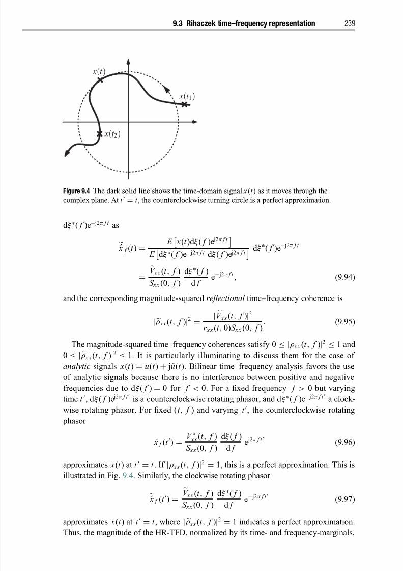
8/21/2019 Statistical Signal Processing of Complex-Valued Data.pdf
http://slidepdf.com/reader/full/statistical-signal-processing-of-complex-valued-datapdf 261/330
9.3 Rihaczek time–frequency representation 239
x(t )
x(t 1)
x(t 2)
Figure 9.4 The dark solid line shows the time-domain signal x (t ) as it moves through the
complex plane. At t = t , the counterclockwise turning circle is a perfect approximation.
d ξ ∗( f )e− j2π f t as
x f (t ) = E x(t )d ξ ( f )e j2π f t
E d ξ ∗( f )e− j2π f t d ξ ( f )e j2π f t
d ξ ∗( f )e− j2π f t
=V x x (t , f )
S x x (0, f )
d ξ ∗( f )
d f e− j2π f t , (9.94)
and the corresponding magnitude-squared reflectional time–frequency coherence is
|ρ x x (t , f )|2 = | V x x (t , f )|2r x x (t , 0)S x x (0, f )
. (9.95)
The magnitude-squared time–frequency coherences satisfy 0 ≤ |ρ x x (t , f )|2 ≤ 1 and
0 ≤ |ρ x x (t , f )|2 ≤ 1. It is particularly illuminating to discuss them for the case of
analytic signals x(t ) = u(t ) + ju(t ). Bilinear time–frequency analysis favors the use
of analytic signals because there is no interference between positive and negative
frequencies due to d ξ ( f ) = 0 for f < 0. For a fixed frequency f > 0 but varying
time t , d ξ ( f )e j2π f t
is a counterclockwise rotating phasor, and d ξ ∗( f )e− j2π f t
a clock-wise rotating phasor. For fixed (t , f ) and varying t , the counterclockwise rotating
phasor
ˆ x f (t ) = V ∗ x x (t , f )
S x x (0, f )
d ξ ( f )
d f e j2π f t (9.96)
approximates x(t ) at t = t . If |ρ x x (t , f )|2 = 1, this is a perfect approximation. This is
illustrated in Fig. 9.4. Similarly, the clockwise rotating phasor
x f (t ) = V x x (t , f )
S x x (0, f )
d ξ ∗( f )
d f e− j2π f t
(9.97)
approximates x(t ) at t = t , where |ρ x x (t , f )|2 = 1 indicates a perfect approximation.
Thus, the magnitude of the HR-TFD, normalized by its time- and frequency-marginals,
8/21/2019 Statistical Signal Processing of Complex-Valued Data.pdf
http://slidepdf.com/reader/full/statistical-signal-processing-of-complex-valued-datapdf 262/330
240 Nonstationary processes
measures how well the time-domain signal x(t ) can be approximated by counterclock-
wise rotating phasors. Similarly, the magnitude of the CR-TFD, normalized by the
time- and frequency-marginals of the HR-TFD, measures how well the time-domain
signal x(t ) can be approximated by clockwise rotating phasors. This suggests that the
distribution of coherence (rather than energy or power) over time and frequency is a
fundamental descriptor of a nonstationary signal.
Finally we point out that, if x (t ) is WSS, the estimator ˆ x f (t ) simplifies to
ˆ x f (t ) = d ξ ( f )e j2π f t (9.98)
for all t , which has already been shown in Section 8.4.2. Furthermore, since WSS
analytic signals are proper, the conjugate-linear estimator is identically zero: x f (t ) = 0
for all t . Hence, WSS analytic signals can be estimated only from counterclockwise
rotating phasors, whereas nonstationary improper analytic signals may also be estimated from clockwise rotating phasors.
9.3.2 Kernel estimators
The Rihaczek distribution is a mathematical expectation. As a practical matter, it must
be estimated. Because such an estimator is likely to be implemented digitally, we present
it for a time series x [k ]. We require that our estimator be a bilinear function of x [k ] that
is covariant with respect to shifts in time and frequency. Estimators that satisfy these
properties constitute Cohen’s class.
10
(Since we want to perform time- and frequency-smoothing, we do not expect our estimator to have the correct time- and frequency-
marginals.) The discrete-time version of Cohen’s class is
V x x [k , θ ) =
m
µ
x[k + m + µ]φ[m, µ] x∗[k + m]e− jµθ , (9.99)
where m is a global and µ a local time variable. The choice of the dual-time kernel
φ[m, µ] determines the properties of the HR-TFD estimator V x x [k , θ ). Omitting the
conjugation in (9.99) gives an estimator of the CR-TFD. It is our objective to design
a suitable kernel φ[m, µ]. A factored kernel that preserves the spirit of the Rihaczek
distribution is
φ[m, µ] = w1[m + µ]w2[µ]w∗3[m]. (9.100)
In practice, the three windows w1, w2, and w3 might be chosen real and even. By
inserting (9.100) into (9.99), we obtain
V x x [k , θ ) =
m
w∗3[m] x∗[k + m]
π
−π
W 2(ω) F 1[k , θ − ω)e jm(θ −ω) d ω
2π. (9.101)
Here W 2(ω) is the discrete-time Fourier transform (DTFT) of w2[µ] and F 1 is theshort-time Fourier transform (STFT) of x [k ] using window w1, defined as
F 1[k , θ ) =
n
w1[n] x[n + k ]e− jnθ . (9.102)
8/21/2019 Statistical Signal Processing of Complex-Valued Data.pdf
http://slidepdf.com/reader/full/statistical-signal-processing-of-complex-valued-datapdf 263/330
9.3 Rihaczek time–frequency representation 241
The corresponding expression for the CR-TFD estimator is obtained by omitting the two
conjugations in (9.101).
In the estimator (9.101), the STFT F 1[k , θ − ω)e jm(θ −ω) plays the role of d ξ (θ )e jk θ
in the CL spectral representation. The STFT is averaged over time with window w3[k ]
and over frequency with window W 2(ω). Thus, the three windows play different roles.
Window w1 should be a smooth tapering window to stabilize the STFT F 1, whereas
the windows w3 and W 2 should be localized to concentrate the estimator in time and
frequency, respectively. A computationally efficient implementation of this estimator
was presented by Hindberg et al . (2006). Choosing φ[m, µ] = δ[m], i.e., w1[n] = 1,
w2[µ] = 1, and w3[m] = δ[m], produces an instantaneous estimator of the Rihaczek
distribution without any time- or frequency-smoothing.
Statistical propertiesFrom (9.99) we find that
E V x x [k , θ ) =
m
µ
φ[m, µ]r x x [k + m, µ]e− jµθ
=
m
π
−π
V x x [m, ω)[m − k , θ − ω)d ω
2π, (9.103)
where r x x [k , κ] = E ( x[k + κ] x∗[k ]) and [m, ω) is the DTFT of φ[m, µ] in µ. For the
factored kernel (9.100) we have
[m, ω) = w∗3[m]
π
−π
W 2(ω − ν)W 1(ν)e jmν d ν
2π. (9.104)
The mean (9.103) of the HR-TFD estimator is thus a time–frequency-smoothed
version of the Rihaczek distribution. The same result holds for the CR-TFD
estimator.
In order to derive the second-order properties of the estimator, we assume Gaussian
signals. This avoids the appearance of fourth-order terms (cf. Section 2.5.3). An exact
expression for the covariance of the HR-TFD estimator is11
cov{ V x x [k 1, θ 1), V x x [k 2, θ 2)}
=
m1
m2
µ1
µ2
φ[m1, µ1]φ∗[m2, µ2]e− j(µ1θ 1−µ2θ 2)
× {r x x [k 1 + m1 + µ1, k 2 − k 1 + m2 − m1 + µ2 − µ1]
× r ∗ x x [k 1 + m1, k 2 − k 1 + m2 − m1] + r x x [k 1 + m1, k 2 − k 1 + m2 − m1 + µ2]
× r ∗ x x [k 1 + m1 + µ1, k 2 − k 1 + m2 − m1 − µ1]}.
We observe that the covariance of the HR-TFD estimator in general depends on both the
Hermitian and thecomplementary correlation. The covariance of the CR-TFD estimator,
8/21/2019 Statistical Signal Processing of Complex-Valued Data.pdf
http://slidepdf.com/reader/full/statistical-signal-processing-of-complex-valued-datapdf 264/330
242 Nonstationary processes
on the other hand, depends on the Hermitian correlation only:
cov{
V x x [k 1, θ 1),
V x x [k 2, θ 2)}
=m1
m2
µ1
µ2
φ[m1, µ1]φ∗[m2, µ2]e− j(µ1θ 1−µ2θ 2)
× {r x x [k 1 + m1 + µ1, k 2 − k 1 + m2 − m1 + µ2 − µ1]
× r x x [k 1 + m1, k 2 − k 1 + m2 − m1] + r x x [k 1 + m1, k 2 − k 1 + m2 − m1 + µ2]
× r x x [k 1 + m1 + µ1, k 2 − k 1 + m2 − m1 − µ1]}.
We can derive the following approximate expression for the variance of the HR-
TFD estimator, assuming analytic and quasi-stationary signals whose time duration of
stationarity is much greater than the duration of correlation:
var { V x x [k , θ )} ≈
m
π
0
|[m − k , θ − ω)|2 |V x x [k , ω)|2
+ [m − k , θ − ω)∗[m − k , θ + ω) | V x x [k , ω)|2 d ω
2π.
(9.105)
However, the same simplifying approximation of large duration of stationarity leads to a
vanishing CR-TFD estimator because stationary analytic signals have zero complemen-tary correlation. This result should not be taken as an indication that the CR-TFD is not
important for analytic signals. Rather it shows that the assumption of quasi-stationarity
with large duration of stationarity is a rather crude approximation to the general class of
nonstationary signals.
9.4 Rotary-component and polarization analysis
In Section 9.3.1, we determined the LMMSE estimator of the time-domain signal at afixed time instant t from the frequency-domain representation at a fixed frequency f .
This showed us how well the signal can be approximated from clockwise or counter-
clockwise turning circles (phasors). It thus seems natural to ask how well the signal can
be approximated from ellipses, which combine the contributions from clockwise and
counterclockwise circles. This framework will allow us to extend rotary-component and
polarization analysis from the stationary case, described in Section 8.4, to a nonstation-
ary setting.12 We thus construct a WLMMSE estimator of x(t ), for fixed t , from the
frequency-domain representation at + f and − f , where throughout this entire section
f shall denote a fixed nonnegative frequency:
ˆ x f (t ) = W 1(t , f )d ξ ( f )e j2π f t + W 2(t ,− f )d ξ ∗( f )e− j2π f t
+ W 1(t ,− f )d ξ (− f )e− j2π f t + W 2(t , f )d ξ ∗(− f )e j2π f t . (9.106)
8/21/2019 Statistical Signal Processing of Complex-Valued Data.pdf
http://slidepdf.com/reader/full/statistical-signal-processing-of-complex-valued-datapdf 265/330
9.4 Rotary-component and polarization analysis 243
Since (t , f ) are fixed, W 1(t , f ), W 1(t ,− f ), W 2(t , f ), and W 2(t ,− f ) are four complex
coefficients that are determined such that E | ˆ x f (t ) − x(t )|2 is minimized. By combining
terms with e j2π f t and terms with e− j2π f t , we obtain
ˆ x f (t ) = [W 1(t , f )d ξ ( f )+ W 2(t , f )d ξ ∗(− f )] d ζ (t , f )
e j2π f t
+ [W 1(t ,− f )d ξ (− f )+ W 2(t ,− f )d ξ ∗( f )] d ζ (t ,− f )
e− j2π f t . (9.107)
For fixed (t , f ) but varying t ,
εt , f (t ) = d ζ (t , f )e j2π f t
εt , f +(t )
+ d ζ (t ,− f )e− j2π f t
εt , f − (t )
(9.108)
describes an ellipse in the complex time-domain plane. We may say that the varying
t traces out a local ellipse εt , f (t ) whose parameters are “frozen” for a given (t , f ).
Since εt , f (t ) = ˆ x f (t ), the local ellipse εt , f (t ) provides the best approximation of x (t ) at
t = t . Following the terminology introduced in Section 8.4.1, the local ellipse εt , f (t )is also called the polarization ellipse at (t , f ), and εt , f + (t ) and εt , f − (t ) are the rotary
components.
One ellipse can be constructed for every time–frequency point (t , f ). This raises
the following obvious question: which ellipses in the time–frequency plane should
the analysis focus on? We propose to consider those points (t , f ) where the local
ellipses provide a good approximation of the nonstationary signal x(t ). The quality of
the approximation can be measured in terms of a time–frequency coherence, which is
introduced in the next subsection.
In the WSS case, we found that the WSS ellipse
ε f (t ) = d ξ ( f )e j2π f t + d ξ (− f )e− j2π f t (9.109)
is the WLMMSE estimate of x (t ), for all t , from the rotary components at frequency f .
On comparing the WSS ellipse with the nonstationary solution (9.108), we see that therandom variables d ζ (t , f ) and d ζ (t ,− f ) now play the roles of the spectral increments
d ξ ( f ) and d ξ (− f ) in the WSS ellipse.
In order to determine the optimum coefficients W 1(t ,± f ) and W 2(t ,± f ) in (9.107),
we introduce the short-hand notation
d Ξ(t , f ) =
d ξ ( f )e j2π f t
d ξ ∗(− f )e j2π f t
d ξ (− f )e− j2π f t
d ξ ∗( f )e− j2π f t
. (9.110)
The local ellipse is found as the output of a WLMMSE filter
εt , f (t ) = V x(t , f )K †(t , f )
d Ξ(t , f )
d f , (9.111)
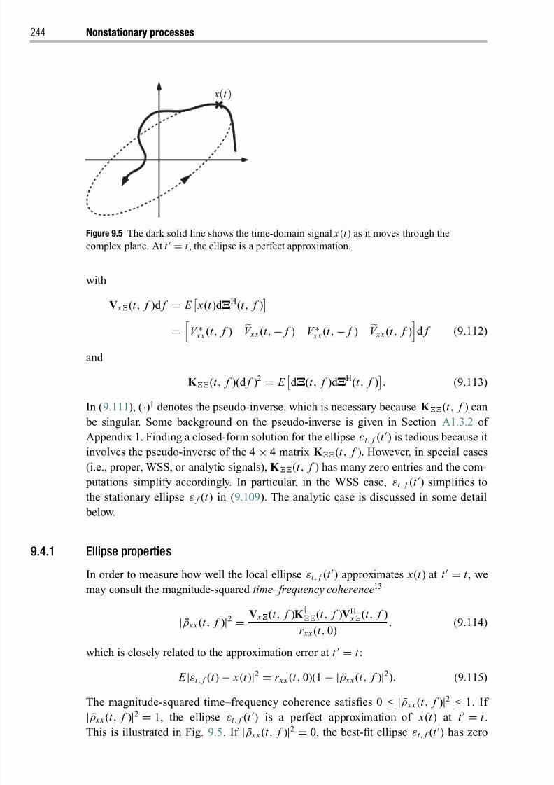
8/21/2019 Statistical Signal Processing of Complex-Valued Data.pdf
http://slidepdf.com/reader/full/statistical-signal-processing-of-complex-valued-datapdf 266/330
244 Nonstationary processes
x(t )
Figure 9.5 The dark solid line shows the time-domain signal x (t ) as it moves through the
complex plane. At t = t , the ellipse is a perfect approximation.
with
V x(t , f )d f = E x(t )d ΞH(t , f )
=
V ∗ x x (t , f ) V x x (t ,− f ) V ∗ x x (t ,− f ) V x x (t , f )d f (9.112)
and
K (t , f )(d f )2 = E d Ξ(t , f )d ΞH(t , f )
. (9.113)
In (9.111), (·)† denotes the pseudo-inverse, which is necessary because K (t , f ) can be singular. Some background on the pseudo-inverse is given in Section A1.3.2 of
Appendix 1. Finding a closed-form solution for the ellipse εt , f (t ) is tedious because it
involves the pseudo-inverse of the 4 × 4 matrix K (t , f ). However, in special cases
(i.e., proper, WSS, or analytic signals), K (t , f ) has many zero entries and the com-
putations simplify accordingly. In particular, in the WSS case, εt , f (t ) simplifies to
the stationary ellipse ε f (t ) in (9.109). The analytic case is discussed in some detail
below.
9.4.1 Ellipse properties
In order to measure how well the local ellipse εt , f (t ) approximates x(t ) at t = t , we
may consult the magnitude-squared time–frequency coherence13
|ρ x x (t , f )|2 = V x(t , f )K †(t , f )VH
x(t , f )
r x x (t , 0) , (9.114)
which is closely related to the approximation error at t = t :
E
|εt , f (t )
− x(t )
|2
=r x x (t , 0)(1
− |ρ x x (t , f )
|2). (9.115)
The magnitude-squared time–frequency coherence satisfies 0 ≤ |ρ x x (t , f )|2 ≤ 1. If
|ρ x x (t , f )|2 = 1, the ellipse εt , f (t ) is a perfect approximation of x(t ) at t = t .
This is illustrated in Fig. 9.5. If |ρ x x (t , f )|2 = 0, the best-fit ellipse εt , f (t ) has zero
8/21/2019 Statistical Signal Processing of Complex-Valued Data.pdf
http://slidepdf.com/reader/full/statistical-signal-processing-of-complex-valued-datapdf 267/330
9.4 Rotary-component and polarization analysis 245
amplitude. The time–frequency coherence tells us which regions of the time–frequency
plane our analysis should focus on: these are the points (t , f ) that have magnitude-
squared coherence close to 1.
As we have seen above, the random variables d ζ (t , f ) and d ζ (t ,−
f ) in the nonsta-
tionary case play the roles of the spectral increments d ξ ( f ) and d ξ (− f ) in the WSS
case. The properties of the local ellipse may therefore be analyzed using the augmented
ESD matrix Jεε
(t , f ) defined by
Jεε
(t , f )(d f )2 =
J εε (t , f ) ˜ J εε(t , f )˜ J ∗εε (t , f ) J εε(t ,− f )
(d f )2 (9.116)
= E
|d ζ (t , f )|2 d ζ (t , f )d ζ (t ,− f )
d ζ ∗(t , f )d ζ ∗(t ,− f ) |d ζ (t ,− f )|2
, (9.117)
instead of the augmented PSD matrixP x x ( f ) in the WSScase.14 Just as in the WSS case
discussed in Section 8.4.2, the expected orientation of the ellipse is then approximated
by
tan(2ψ(t , f )) = Im ˜ J εε(t , f )
Re ˜ J εε(t , f )(9.118)
and the area by
π | J εε(t , f )− J εε(t ,− f )|(d f )2, (9.119)
and its shape is approximately characterized by
sin(2χ(t , f )) = J εε (t , f )− J εε(t ,− f )
J εε (t , f )+ J εε(t ,− f ). (9.120)
The analysis of polarization and coherence proceeds completely analogously to Sec-
tion 8.4.3. For instance, as in (8.79), the degree of polarization is
(t , f ) =
1 − 4det Jεε
(t , f )
tr 2Jεε
(t , f ) . (9.121)
9.4.2 Analytic signals
For analytic signals, these expressions simplify. If x (t ) is analytic, d ξ (− f ) = 0 and the
local ellipse becomes
εt , f (t ) = W 1(t , f )d ξ ( f ) d ζ (t , f )
e j2π f t + W 2(t ,− f )d ξ ∗( f ) d ζ (t ,− f )
e− j2π f t . (9.122)
Thus,
Jεε
(t , f )(d f )2 = E
W 1(t , f )d ξ ( f )
W ∗2 (t ,− f )d ξ ( f )
W ∗1 (t , f )d ξ ∗( f ) W 2(t ,− f )d ξ ∗( f )
(9.123)
8/21/2019 Statistical Signal Processing of Complex-Valued Data.pdf
http://slidepdf.com/reader/full/statistical-signal-processing-of-complex-valued-datapdf 268/330
246 Nonstationary processes
and then
Jεε
(t , f ) = S x x (0, f )
|W 1(t , f )|2 W 1(t , f )W 2(t ,− f )
W ∗1 (t , f )W ∗2 (t ,− f ) |W 2(t ,− f )|2
. (9.124)
From (9.111), we determine the filter coefficients
W 1(t , f )d f = V ∗ x x (t , f )S x x (0, f )− V x x (t , f )S ∗ x x (2 f , f )e− j4π f t
S 2 x x (0, f )− |S x x (2 f , f )|2, (9.125)
W 2(t ,− f )d f =V x x (t , f )S x x (0, f )− V ∗ x x (t , f )S x x (2 f , f )e j4π f t
S 2 x x (0, f )− |S x x (2 f , f )|2, (9.126)
provided that S 2 x x (0, f ) = |
S x x (2 f , f )|2. If S 2 x x (0, f ) = |
S x x (2 f , f )|2, then d ξ ∗( f ) =
e jα d ξ ( f ) for some real α and the WLMMSE estimator becomes strictly linear. We find
for this special case
W 1(t , f )d f = V ∗ x x (t , f )
S x x (0, f ), (9.127)
W 2(t ,− f )d f = 0, (9.128)
which makes the approximating ellipse a circle.
It is interesting to examine the ellipse shape and polarization, which, for S 2 x x (0, f ) =|
S x x (2 f , f )|2, can be done through the angle χ (t , f ) defined by
sin(2χ(t , f )) = (|V x x (t , f )|2
− | V x x (t , f )|2
)(S
2
x x (0, f )− |S x x (2 f , f )|2
) D
, (9.129)
where
D = (|V x x (t , f )|2 + | V x x (t , f )|2)(S 2 x x (0, f )+ |S x x (2 f , f )|2)
− 4 Re
V ∗ x x (t , f )V ∗ x x (t , f )S x x (0, f )S x x (2 f , f )e j4π f t
.
If x(t ) is proper at time t and frequency f ,
V x x (t , f ) = 0 and
S x x (2 f , f ) = 0, then
χ(t , f ) = π/4. This says that a proper analytic signal is counterclockwise circularly
polarized . On the other hand, if S 2 x x (0, f ) = |S x x (2 f , f )|2, then d ξ ∗( f ) = e jα d ξ ( f ) and thus |V x x (t , f )|2 = | V x x (t , f )|2. In thiscase, the signal x(t ) can beregarded asmaximally
improper at frequency f . A maximally improper analytic signal has χ (t , f ) = π/4 and
is therefore also counterclockwise circularly polarized .
Since det Jεε
(t , f ) = 0 for all (t , f ), all analytic signals are completely polarized .
Yet, while |S x x (2 f , f )|2 ≤ S 2 x x (0, f ), the magnitude of the HR-TFD does not provide an
upper bound on the magnitude of the CR-TFD, i.e., | V x x (t , f )|2 |V x x (t , f )|2. More-
over, |V x x (t , f )|2 = |
V x x (t , f )|2 does not imply S 2 x x (0, f ) = |
S x x (2 f , f )|2. Therefore it
is possible that x (t ) is clockwise polarized at (t , f ), i.e., χ (t , f ) < 0, provided that the
signal is “sufficiently improper” at (t , f ). This result may seem surprising, consideringthat an analytic signal is synthesized from counterclockwise phasors only.
The quality of the approximation can be judged by computing the magnitude-squared
time–frequency coherence |ρ x x (t , f )|2 defined in (9.114). For analytic signals, we obtain
8/21/2019 Statistical Signal Processing of Complex-Valued Data.pdf
http://slidepdf.com/reader/full/statistical-signal-processing-of-complex-valued-datapdf 269/330
9.5 Higher-order statistics 247
the simplified expression
|ρ x x (t , f )|2 = N
r x x (t , 0)(S 2 x x (0, f )
− |S x x (2 f , f )
|2),
(9.130)
where
N = S x x (0, f )(|V x x (t , f )|2 + | V x x (t , f )|2)
− 2 Re[V ∗ x x (t , f )V ∗ x x (t , f )S x x (2 f , f )e j4π f t ],
if S 2 x x (0, f ) = |S x x (2 f , f )|2. Both in the proper case, which is characterized byV x x (t , f ) = 0 and S x x (2 f , f ) = 0, and in the maximally improper case, characterized by
S 2 x x (0, f ) = |
S x x (2 f , f )|2, the magnitude-squared time–frequency coherence simplifies
to the magnitude-squared rotational time–frequency coherence (9.93), i.e.,
|ρ x x (t , f )|2 = |ρ x x (t , f )|2 = |V x x (t , f )|2r x x (t , 0)S x x (0, f )
. (9.131)
In thesecases x(t ) canbe estimatedfrom counterclockwise rotating phasors only. In other
words, the optimum WLMMSEestimator is theLMMSE estimator, i.e., W 2(t ,− f ) = 0.
9.5 Higher-order statistics
We conclude this chapter with a very brief introduction to the higher-order statistics of a continuous-time signal x (t ).15 We denote the nth-order moment function by
m x,♦(t , ) = E
xn (t )
n−1i=1
xi (t + τ i )
, (9.132)
where, as in Section 8.5, = [τ 1, . . . , τ n−1]T, and ♦ = [n ,1,2, . . . ,n−1]T contains
elements i that are either 1 or the conjugating star ∗. This leads to 2n different nth-order
moment functions, depending on which terms are conjugated. As explained in Section
8.5, not all of these functions are required for a complete statistical description.
We assume that x (t ) can be represented as in the CL spectral representation (9.47),
x(t ) = ∞−∞
d ξ ( f )e j2π f t , (9.133)
but ξ ( f ) is now an N th-order spectral process with moments defined and bounded up
to N th order. That is, the moment functions can be expressed in terms of the increment
process d ξ ( f ) as
m x,♦(t , ) =
IR n E
d ξ n (− n f n)
n−1
i=1
d ξ i (i f i )
e j2π[f T+( f 1+···+ f n−1− f n)t ], (9.134)
where n = 1, . . . , N , f = [ f 1, . . . , f n−1]T, and i f i = −1 if i is the conjugation star ∗.
The “−” sign for f n is to ensure that (9.134) complies with (9.50) and (9.51) in the
second-order case n = 2. Since t is a global time variable and contains local time
8/21/2019 Statistical Signal Processing of Complex-Valued Data.pdf
http://slidepdf.com/reader/full/statistical-signal-processing-of-complex-valued-datapdf 270/330
248 Nonstationary processes
lags, we call f 1, . . . , f n−1 global frequencies and ν = f 1 + · · · + f n−1 − f n = f T1 − f n
a local frequency-offset. With this substitution, we obtain
m x,♦(t , ) = IR n E d ξ n
(n(ν − f T
1))
n−1
i=1
d ξ i
(i f i ) e j2π (f T
+νt )
. (9.135)
We now define
S x,♦(ν, f )d ν d n−1f = E
d ξ n (n(ν − f T1))
n−1i=1
d ξ i (i f i )
. (9.136)
We call S x,♦(ν, f ) the nth-order spectral correlation, which we recognize as the n-
dimensional Fourier transform of the moment function m x,♦(t , ). The spectral corre-
lation may contain δ-functions (e.g., in the stationary case).
Consider now a signal x (t ) that is stationary up to order N . Then none of the momentfunctions m x,♦(t , ), for n = 1, . . . , N and arbitrary ♦, depends on t : m x,♦(t , ) =m x ,♦( ). This can be true only if S x,♦(ν, f ) is zero outside the stationary manifold
ν = 0. The (n − 1)-dimensional Fourier transform of m x,♦( )
M x ,♦(f ) =
IR n−1
m x,♦( )e− j2π f T d n−1 , (9.137)
is the nth-order moment spectrum introduced in (8.97). The moment spectrum and
spectral correlation of a stationary process are related as
S x ,♦(ν, f ) = M x ,♦(f )δ(ν). (9.138)
The moment spectrumcan be expressed directly in termsof the increments of the spectral
process as
M x,♦(f ) d n−1f = E
d ξ n (− n f T1)
n−1i=1
d ξ i (i f i )
. (9.139)
Notes
1 Section 9.1 closely follows the presentation by Schreier et al . (2005). This paper is cIEEE,
and portions are reused with permission.
2 For Grenander’s theorem, see for instance, Section VI.B.2 in Poor (1998).
3 Section 9.2 draws on material presented by Picinbono and Bondon (1997) and Schreier and
Scharf (2003b).
4 Note that Schreier and Scharf (2003b) use a slightly different way of defining global and
local variables: they define t 1 = t , t 2 = t − τ and thus f 1 = f + ν, f 2 = f , whereas we define
t 1 = t + τ , t 2 = t and thus f 1 = f , f 2 = f − ν. While this leads to results that look slightly
different, they are fundamentally the same.
5 The Rihaczek distribution for deterministic signals was introduced by Rihaczek (1968). The
extension to stochastic signals that is based on harmonizability is due to Martin (1982).
Note that we do not follow the (somewhat confusing) convention of differentiating between
time–frequency representations for deterministic and stochastic signals by calling the former
8/21/2019 Statistical Signal Processing of Complex-Valued Data.pdf
http://slidepdf.com/reader/full/statistical-signal-processing-of-complex-valued-datapdf 271/330
Notes 249
“distributions” and the latter “spectra.” Time–frequency distributions for stochastic signals in
general are discussed by Flandrin (1999), and the Rihaczek distribution in particular by Scharf
et al . (2005).
6 For a discussion of Wigner’s theorem and its consequences for time–frequency analysis, see
Flandrin (1999).7 The Wigner–Ville distribution is the Fourier transform (in τ ) of E [ x(t + τ /2) x (∗)(t − τ/2)].
That is, the local time lag τ is split symmetrically between t 1 = t + τ/2 and t 2 = t − τ/2,
which leads to a symmetric split of the frequency-offset ν between the frequency variables
f 1 = f + ν/2 and f 2 = f − ν/2. For a thorough treatment of the Wigner–Ville distribution,
see Flandrin (1999).
8 Estimating x(t ) from the random variable d ξ ( f )e j2π f t assumes that x(t ) is an energy signal
whose Fourier transform X ( f ) = d ξ ( f )/d f exists. If x(t ) is not an energy signal, we must
estimate the increment x (t )d f instead. This requires only minor changes to the remaining
development in Sections 9.3 and 9.4.
9 Following the terminology introduced in Chapter 4, ρ x x (t , f ) is a rotational correlation coef-
ficient between x(t ) and d ξ ( f )e j2π f t , at fixed t and f . However, in this context, the term“coherence” is preferred over “correlation coefficient.” The time–frequency coherence should
not be confused with the coherence introduced in Definition 8.2, which is a frequency-domain
coherence between the rotary components at a given frequency. The time–frequency coherence
does not simplify to the frequency-domain coherence for a WSS signal.
10 Cohen’s class was introduced in quantum mechanics by Cohen (1966). Members of this class
can also be regarded as estimators of the Wigner–Ville distribution, see Martin and Flandrin
(1985). The estimator of Section 9.3.2 was presented by Scharf et al . (2005), building upon
prior work by Scharf and Friedlander (2001). The paper Scharf et al . (2005) is cIEEE, and
portions are reused with permission.
11 The evaluation of the statistical properties of the HR/CR -TFD estimators is due to Scharf et al .
(2005), following the lead of Martin and Flandrin (1985). Note again that the results presented
in Section 9.3.2 look different at first than those of Scharf et al . (2005) even though they
are really identical. This is because Scharf et al . (2005) define r x x [k , κ] = E ( x[k ] x∗[k − κ]),
whereas this book defines r x x [k , κ] = E ( x[k + κ] x∗[k ]).
12 Section 9.4 follows Schreier (2008b). The paper is cIEEE, and portions are reused with
permission. Previous extensions of rotary-component and polarization analysis to non-
stationary signals have been centered mainly around the wavelet transform, and to a
much lesser extent, the STFT. The interested reader is referred to Lilly and Park (1995),
Olhede and Walden (2003a, 2003b), Lilly and Gascard (2006), and Roueff et al . (2006).
13 In the language of Chapter 4, ρ x x (t , f ) is a total correlation coefficient between x(t ) and
[d ξ ( f )e j2π f t , d ξ (−
f )e− j2π f t ].
14 This assumes that x (t ) is an energy signal with bounded ESD. If x (t ) is a power signal, we have
to work with PSDs instead. That is, instead of using J εε(t , f )(d f )2 = E |d ζ (t , f )|2, we use
P εε (t , f )d f = E |d ζ (t , f )|2. This requires only minor changes in the remainder of the section.
15 A detailed discussion of higher-order statistics for nonstationary signals (albeit real-valued) is
given by Hanssen and Scharf (2003).
8/21/2019 Statistical Signal Processing of Complex-Valued Data.pdf
http://slidepdf.com/reader/full/statistical-signal-processing-of-complex-valued-datapdf 272/330
10 Cyclostationary processes
Cyclostationary processes are an important class of nonstationary processes that have
periodically varying correlation properties. They can model periodic phenomena occur-
ring in science and technology, including communications (modulation, sampling, and
multiplexing), meteorology, oceanography, climatology, astronomy (rotation of the Earth
and other planets), and economics (seasonality). While cyclostationarity can manifest
itself in statistics of arbitrary order, we will restrict our attention to phenomena in which
the second-order correlation and complementary correlation functions are periodic in
their global time variable.
Our program for this chapter is as follows. In Section 10.1, we discuss the spectral
properties of harmonizable cyclostationary processes. We have seen in Chapter 8 that
the second-order averages of a WSS process are characterized by the power spectral
density (PSD) and complementary power spectral density (C-PSD). These each cor-
respond to a single δ-ridge (the stationary manifold) in the spectral correlation and
complementary spectral correlation. Cyclostationary processes have a (possibly count-
ably infinite) number of so-called cyclic PSDs andC-PSDs. These correspond to δ-ridges
in the spectral correlation and complementary spectral correlation that are parallel to
the stationary manifold. In Section 10.2, we derive the cyclic PSDs and C-PSDs of
linearly modulated digital communication signals. We will see that there are two types
of cyclostationarity: one related to the symbol rate, the other to impropriety and carrier
modulation.
Because cyclostationary processes are spectrally correlated between different fre-
quencies, they have spectral redundancy. This redundancy can be exploited in optimumestimation. The widely linear minimum mean-squared error filter is called the cyclic
Wiener filter , which is discussed in Section 10.3. It can be considered the cyclostation-
ary extension of the WSS Wiener filter. The cyclic Wiener filter consists of a bank of
linear shift-invariant filters that are applied to frequency-shifted versions of the signal
and its conjugate. In Section 10.4, we develop an efficient causal filter-bank implemen-
tation of the cyclic Wiener filter for cyclostationary discrete-time series, which is based
on a connection between scalar-valued cyclostationary and vector-valued WSS time
series.
We need to emphasize that, due to space constraints, we can barely scratch the surfaceof the very rich topic of cyclostationarity in this chapter. For further information, we refer
the reader to the review article by Gardner et al . (2006) and the extensive bibliography
by Serpedin et al . (2005).
8/21/2019 Statistical Signal Processing of Complex-Valued Data.pdf
http://slidepdf.com/reader/full/statistical-signal-processing-of-complex-valued-datapdf 273/330
10.1 Characterization and spectral properties 251
10.1 Characterization and spectral properties
Cyclostationary processes have a correlation function r x x (t , τ ) = E [ x(t + τ ) x∗(t )] and
complementary correlation function r x x (t , τ ) = E [ x(t + τ ) x(t )] that are both periodicin their global time variable t .
Definition 10.1. A zero-mean process x(t ) is cyclostationary (CS) if there exists T > 0
such that
r x x (t , τ ) = r x x (t + T , τ ), (10.1)
r x x (t , τ ) = r x x (t + T , τ ) (10.2)
for all t and τ .
CS processes are sometimes also called periodically correlated . If x (t ) does not have
zero mean, we require that the mean be T -periodic as well, i.e., µ x (t ) = µ x (t + T ) for
all t . Note that r x x (t , τ ) might actually be T 1-periodic and r x x (t , τ ) T 2-periodic. The
period T would then be the least common multiple of T 1 and T 2. It is important to stress
that the periodicity is in the global time variable t , not the local time offset τ . Periodicity
in τ may occur independently of periodicity in t . It should also be emphasized that
periodicity refers to the correlation and complementary correlation functions, not the
process itself. That is, in general, x (t ) = x(t + T ).
For WSS processes, (10.1) and (10.2) hold for arbitrary T > 0. Thus, WSS pro-cesses are a subclass of CS processes. The CS processes we consider are more pre-
cisely called wide-sense (or second-order) CS, since Definition 10.1 considers only
second-order statistics. A process can also be higher-order CS if higher-order correla-
tion functions are periodic in t , and strict-sense CS if the probability density function is
periodic in t .
Adding two uncorrelated CS processes with periods T 1 and T 2 produces another CS
process whose period is the least common multiple (LCM) of T 1 and T 2. However, if the
two periods are incommensurate, e.g., T 1 = 1 and T 2 = π , then the LCM is ∞. Such a
process is CS in a generalized sense, which is called almost CS because its correlationfunction is an almost periodic function in the sense of Bohr. For fixed τ , the correlation
and complementary correlation functions of an almost CS process are each a possibly
infinite sum of periodic functions. Many of the results for CS processes generalize to
almost CS processes.
10.1.1 Cyclic power spectral density
We now discuss the spectral properties of harmonizable CS processes, which possess
a Cramer–Loeve (CL) spectral representation (cf. Section 9.2). The spectral correla-tion and complementary correlation are the two-dimensional Fourier transforms of the
time correlation and complementary correlation function. However, since r x x (t , τ ) and
r x x (t , τ ) are periodic in t , we compute the Fourier series coefficients rather than the
8/21/2019 Statistical Signal Processing of Complex-Valued Data.pdf
http://slidepdf.com/reader/full/statistical-signal-processing-of-complex-valued-datapdf 274/330
252 Cyclostationary processes
Fourier transform in t . These Fourier series coefficients are
p x x (n/ T , τ ) = 1
T T
0
r x x (t , τ )e− j2π nt / T d t , (10.3)
˜ p x x (n/ T , τ ) = 1
T
T
0
r x x (t , τ )e− j2π nt / T d t , (10.4)
and they are called the cyclic correlation function and cyclic complementary correlation
function, respectively. There is a subtle differencebetween the cyclic correlation function
and the ambiguity function, which is defined as the Fourier transform of the correlation
function in t (see Section 9.2.1). The cyclic correlation function and the ambiguity
function have different physical units.
The Fourier transform of the cyclic correlation and cyclic complementary correlation
functions in τ yields the cyclic power spectral density and cyclic complementary power spectral density:
P x x (n/ T , f ) = ∞−∞
p x x (n/ T , τ )e− j2π f τ d τ, (10.5)
P x x (n/ T , f ) = ∞−∞
˜ p x x (n/ T , τ )e− j2π f τ d τ. (10.6)
The appropriate generalization for the cyclic correlation and complementary correla-
tion of almost CS processes is
p x x (νn , τ ) = limT →∞
1
T
T /2
−T /2
r x x (t , τ )e− j2π νn t d t , (10.7)
˜ p x x (νn , τ ) = limT →∞
1
T
T /2
−T /2
r x x (t , τ )e− j2π νn t d t . (10.8)
The frequency offset variables νn and νn are called the cycle frequencies. The set
of cycle frequencies {νn} for which p x x (νn , τ ) is not identically zero and the set of
cycle frequencies
{νn
} for which ˜ p x x (νn , τ ) is not identically zero are both count-
able (but possibly countably infinite). These two sets do not have to be identical. CS processes are a subclass of almost CS processes in which the frequencies {νn} and
{νn} are contained in a lattice of the form {n/ T }. Relationships (10.5) and (10.6)
remain valid for almost CS processes if n/ T is replaced with the cycle frequencies νn
and νn:
P x x (νn , f ) = ∞−∞
p x x (νn , τ )e− j2π f τ d τ, (10.9)
P x x (νn , f )
= ∞
−∞˜ p x x (νn , τ )e− j2π f τ d τ. (10.10)
Harmonizable signals may be expressed as
x(t ) = ∞−∞
d ξ ( f )e j2π f t . (10.11)
8/21/2019 Statistical Signal Processing of Complex-Valued Data.pdf
http://slidepdf.com/reader/full/statistical-signal-processing-of-complex-valued-datapdf 275/330
10.1 Characterization and spectral properties 253
The next result for harmonizable almost CS processes, which follows immediately from
the CL spectral representation in Result 9.2, connects the cyclic PSD and C-PSD to the
second-order properties of the increments of the spectral process ξ ( f ).
Result 10.1. The cyclic PSD P x x (νn , f ) can be expressed as
P x x (νn , f )d f = E [d ξ ( f )d ξ ∗( f − νn)], (10.12)
and the cyclic C-PSD P x x (νn, f ) as P x x (νn , f )d f = E [d ξ ( f )d ξ (νn − f )]. (10.13)
Moreover, the spectral correlation S x x (ν, f ) and the complementary spectral corre-
lation
S x x (ν, f ), defined in Result 9.2, contain the cyclic PSD and C-PSD on δ-ridges
parallel to the stationary manifold ν = 0:
S x x (ν, f ) =n
P x x (νn , f )δ(ν − νn), (10.14)
S x x (ν, f ) =
n
P x x (νn , f )δ(ν − νn). (10.15)
On the stationary manifold ν = 0, the cyclic PSD is the usual PSD, i.e., P x x (0, f ) = P x x ( f ), and the cyclic C-PSD the usual C-PSD, i.e., P x x (0, f ) = P x x ( f ). It is clear from
the bounds in Result 9.3 that it is not possible for the spectral correlation S x x (ν, f ) to
have only δ-ridges for ν = 0. CS processes must always have a WSS component, i.e.,
they must have a PSD P x x ( f ) ≡ 0. However, it is possible that a process has cyclic PSD P x x (ν, f ) ≡ 0 for all ν = 0 but cyclic C-PSD P x x (νn, f ) ≡ 0 for some νn = 0.
Example 10.1. Let u(t ) be a real WSS random process with PSD P uu ( f ). The complex-
modulated process x(t ) = u(t )e j2π f 0t has PSD P x x ( f ) = P uu ( f − f 0) and cyclic PSD
P x x (ν, f ) ≡ 0 for all ν = 0. However, x(t ) is CS rather than WSS because the cyclic
C-PSD is nonzero outside the stationary manifold for ν = 2 f 0: P x x (2 f 0, f ) = P uu ( f − f 0).
Unfortunately, there is not universal agreement on the nomenclature for CS processes.
It is also quite common to call the cyclic PSD P x x (νn , f ) the “spectral correlation,” a
term that we use for S x x (ν, f ). In the CS literature, one can often find the statement
“only (almost) CS processes can exhibit spectral correlation.” This can thus be translated
as “only (almost) CS processes can have P x x (νn , f ) ≡ 0 for νn = 0,” which means that
S x x (ν, f ) has δ-ridges outside the stationary manifold ν = 0. However, there also exist
processes whose S x x (ν, f ) have δ-ridges that are curves (not necessarily straight lines)
in the (ν, f )-plane. These processes have been ter med “generalized almost CS” and
were first investigated by Izzo and Napolitano (1998).
10.1.2 Cyclic spectral coherence
The cyclic spectral coherence quantifies how much the frequency-shifted spectral pro-
cess ξ ( f − νn) tells us about the spectral process ξ ( f ). It is defined as the cyclic
8/21/2019 Statistical Signal Processing of Complex-Valued Data.pdf
http://slidepdf.com/reader/full/statistical-signal-processing-of-complex-valued-datapdf 276/330
254 Cyclostationary processes
PSD, normalized by the PSDs at f and f − νn . There is also a complementary
version.
Definition 10.2. The rotational cyclic spectral coherence of an (almost) CS process is
defined as
ρ x x (νn , f ) = E [d ξ ( f )d ξ ∗( f − νn)] E |d ξ ( f )|2 E |d ξ ( f − νn)|2
= P x x (νn , f )√ P x x ( f ) P x x ( f − νn)
(10.16)
and the reflectional cyclic spectral coherence is
ρ x x (νn , f ) = E [d ξ ( f )d ξ (νn − f )] E |d ξ ( f )|2 E |d ξ (νn − f )|2
= P x x (νn , f )√
P x x ( f ) P x x (νn − f ). (10.17)
The terms “rotational” and “reflectional” are borrowed from the language of Chap-
ter 4, which discusses rotational and reflectional correlation coefficients. Correlationcoefficients in the frequency domain are usually called coherences. It is also possible to
define a total cyclic spectral coherence, which takes into account both Hermitian and
complementary correlations.
The squared magnitudes of the cyclic spectral coherences are bounded as 0 ≤|ρ x x (νn , f )|2 ≤ 1 and 0 ≤ |ρ x x (νn , f )|2 ≤ 1. If |ρ x x (νn , f )|2 = 1 for a given (νn , f ),
then d ξ ( f ) can be perfectly linearly estimated from d ξ ( f − νn). If |ρ x x (νn, f )|2 = 1 for
a given (νn , f ), then d ξ ( f ) can be perfectly linearly estimated from d ξ ∗(νn − f ). Note
that, for νn = 0,
ρ x x (0, f ) is the coherence
ρ x x ( f ) in Definition 8.2. It is also clear that
ρ x x (0, f ) = 1.
10.1.3 Estimating the cyclic power-spectral density
In practice, the cyclic correlation function and cyclic PSD must be estimated from
realizations of the random process. For ergodic WSS processes, ensemble averages can
be replaced by time averages over a single realization. Under certain conditions1 this
is also possible for CS processes. For simplicity, we will consider only the Hermitian
cyclic correlation and PSD in this section. Expressions for the complementary quantities
follow straightforwardly.
Since the correlation function is T -periodic, we need to perform synchronized T -
periodic time-averaging. The correlation function is thus estimated as
r x x (t , τ ) = lim K →∞
1
2 K + 1
K k =− K
x(t + kT + τ ) x∗(t + kT ). (10.18)
In essence, this estimator regards each period of the process as a separate realization.
Consequently, an estimate of the cyclic correlation function is obtained by
ˆ p x x (n/ T , τ ) =1
T T
0 r x x (t , τ )e− j2π nt /T
d t
= limT →∞
1
T
T /2
−T /2
x(t + τ ) x∗(t )e− j2π nt / T d t . (10.19)
8/21/2019 Statistical Signal Processing of Complex-Valued Data.pdf
http://slidepdf.com/reader/full/statistical-signal-processing-of-complex-valued-datapdf 277/330
10.2 Linearly modulated communication signals 255
This estimator has the form of (10.7) without the expected value operator. It can also be
used for almost CS processes if n/ T is replaced with νn .
A straightforward estimator of the cyclic PSD is the cyclic periodogram
x x (νn , f ; t 0, T ) = 1T
X ( f ; t 0, T ) X ∗( f − νn; t 0, T ), (10.20)
where
X ( f ; t 0, T ) = t 0+T /2
t 0−T /2
x(t )e− j2π f t d t (10.21)
is the windowed Fourier transform of x(t ) of length T , centered at t 0. This estimator
is asymptotically unbiased as T → ∞ but not consistent. A consistent estimator of the
cyclic PSD is the infinitely time-smoothed cyclic periodogram
ˆ P t x x (νn , f ) = lim
f →0lim
T →∞1
T t 0+T /2
t 0−T /2
x x (νn , f ; t , 1/ f ) d t (10.22)
or the infinitely frequency-smoothed cyclic periodogram
ˆ P f x x (νn , f ) = lim
f →0lim
T →∞1
f
f + f /2
f − f /2
x x (νn, f ; t 0, T ) d f . (10.23)
The order of the two limitscannotbe interchanged. It can beshownthat the two estimatorsˆ P t x x (νn , f ) and ˆ P f
x x (νn , f ) are equivalent.2
10.2 Linearly modulated digital communication signals
In this section, we derive the cyclic PSD and C-PSD of linearly modulated digital
communication signals such as Pulse AmplitudeModulation (PAM), Phase Shift Keying
(PSK), and Quadrature Amplitude Modulation (QAM).3 We will find that there are two
sources of cyclostationarity: one is related to the repetition of pulses at the symbol
interval, the other to impropriety and carrier modulation.
10.2.1 Symbol-rate-related cyclostationarity
An expression for a digitally modulated complex baseband signal is
x(t ) =∞
k =−∞d k b(t − kT ), (10.24)
where b(t ) is the deterministic transmit pulse shape, T the symbol interval (1/ T is the
symbol rate), and d k a complex-valued WSS random data sequence with correlation
r dd [κ] = E [d k +κ d ∗k ] and complementary correlation r dd [κ] = E [d k +κ d k ]. The correla-
tion function of x (t ) is
r x x (t , τ ) =∞
k =−∞
∞m=−∞
E [d k d ∗m]b(t + τ − kT )b∗(t − mT ). (10.25)
8/21/2019 Statistical Signal Processing of Complex-Valued Data.pdf
http://slidepdf.com/reader/full/statistical-signal-processing-of-complex-valued-datapdf 278/330
256 Cyclostationary processes
With the variable substitution κ = k − m, we obtain
r x x (t , τ ) =∞
κ=−∞
r dd [κ]
∞
m=−∞
b(t + τ − κ T − mT )b∗(t − mT ). (10.26)
It is easy to see that r x x (t , τ ) = r x x (t + T , τ ), and a similar development for the comple-
mentary correlation shows that r x x (t , τ ) = r x x (t + T , τ ). Thus, x(t ) is CS with period
T . The cyclic correlation function is
p x x (n/ T , τ ) = 1
T
T
0
r x x (t , τ )e− j2π nt /T d t
= 1
T
∞
κ
=−∞
r dd [κ]
∞
m
=−∞
T
0
b(t + τ − κ T − mT )b∗(t − mT )e− j2π nt /T d t
= 1
T
∞κ=−∞
r dd [κ]
∞−∞
b(t + τ − κ T )b∗(t )e− j2π nt /T d t . (10.27)
Now we define
φ(n/ T , τ ) = ∞−∞
b(t + τ )b∗(t )e− j2π nt /T d t , (10.28)
whose Fourier transform (n/ T , f ) is the spectral correlation of the deterministic pulse
shape b(t )
←→ B( f ):
(n/ T , f ) = B( f ) B∗( f − n/ T ). (10.29)
Inserting (10.28) into (10.27) yields
p x x (n/ T , τ ) = 1
T
∞κ=−∞
r dd [κ]φ(n/ T , τ − κ T ). (10.30)
Its Fourier transform in τ is the cyclic PSD
P x x (n/ T , f ) =1
T P dd ( f )(n/ T , f ) =1
T P dd ( f ) B( f ) B∗( f − n/ T ), (10.31)
where P dd ( f ) is the PSD of the datasequence d k , which is the discrete-time Fourier trans-
form of r dd [κ]. For n = 0, P x x (0, f ) is the PSD. A completely analogous development
leads to the cyclic C-PSD
P x x (n/ T , f ) = 1
T P dd ( f ) B( f ) B(n/ T − f ), (10.32)
where
P dd ( f ) is the C-PSD of the data sequence d k . For n = 0,
P x x (0, f ) is the C-PSD.
Applying these findings to the special case of an uncorrelated data sequence leads to the
following result.
Result 10.2. If the data sequence d k is uncorrelated with zero mean, variance σ 2d , and
complementary variance σ 2d , then the cyclic PSD and cyclic C-PSD of the linearly
8/21/2019 Statistical Signal Processing of Complex-Valued Data.pdf
http://slidepdf.com/reader/full/statistical-signal-processing-of-complex-valued-datapdf 279/330
10.2 Linearly modulated communication signals 257
modulated baseband signal ( 10.24 ) are
P x x (n/ T , f ) = σ 2d
T B( f ) B∗( f − n/ T ), (10.33)
P x x (n/ T , f ) = σ 2d
T B( f ) B(n/ T − f ). (10.34)
We see that the transmit pulse b(t ) determines not only the bandwidth of x (t ) but also
the number of cycle frequencies for which the cyclic PSD and C-PSD are nonzero.
Example 10.2. In Quaternary Phase Shift Keying (QPSK), the transmitted data are uncor-
related, equally likely d k ∈ {±1,± j}, so that σ 2d = 1 and
σ 2d = 0. This produces a proper
baseband signal x(t ). We will consider two transmit pulse shapes. The first is the rect-
angular pulse
b1(t ) =
1, |t | < T /2,
12
, |t | = T /2,
0, |t | > T /2
with Fourier transform B1( f ) = sin(π f T )/(π f ). Another transmit pulse commonly
employed in digital communications is the Nyquist roll-off (or raised-cosine) pulse with
roll-off factor 0 ≤ α ≤ 1:
b2(t ) = sinc t
T
cos(απ t / T )
1 − 4α2(t / T )2. (10.35)
Its Fourier transform is
B2( f ) =
T , | f | ≤ 1 − α
2T ,
T
2
1 − sin
π T
α
| f | − 1
2T
,
1 − α
2T < | f | ≤ 1 + α
2T ,
0, else.
(10.36)
Figure 10.1(a) shows the magnitude of the cyclic PSD of QPSK for the rectangular
pulse b1(t ), and Fig. 10.1( b) is for the Nyquist pulse b2(t ) with roll-off factor α = 1.
The rectangular pulse b1(t ) is not bandlimited, so the cyclic PSD is spread out over the
entire (ν, f )-plane. The Nyquist pulse b2(t ), on the other hand, has a limited two-sided
bandwidth of 2/ T , and the cyclic PSD is nonzero only for {νn} = { −1/ T , 0, 1/ T }.Since QPSK signals are proper, the cyclic complementary PSD is identically
zero.
In Binary Phase Shift Keying (BPSK), the transmitted data are equally likely d k ∈
{±1
}, so that σ 2d
= σ 2d
=1. The rectangular pulse and the Nyquist roll-off pulse are
both real-valued, which means B( f ) = B∗(− f ). Therefore, the BPSK baseband signalis maximally improper and the cyclic C-PSD equals the cyclic PSD: P x x (n/ T , f ) = P x x (n/ T , f ).
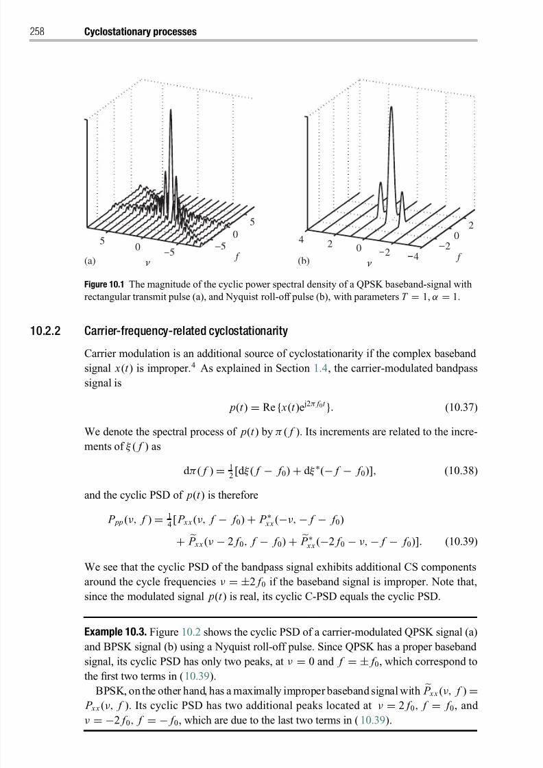
8/21/2019 Statistical Signal Processing of Complex-Valued Data.pdf
http://slidepdf.com/reader/full/statistical-signal-processing-of-complex-valued-datapdf 280/330
258 Cyclostationary processes
0
5
05
(a) (b) f
ν
20
2
42024
f ν
Figure 10.1 The magnitude of the cyclic power spectral density of a QPSK baseband-signal with
rectangular transmit pulse (a), and Nyquist roll-off pulse (b), with parameters T = 1, α = 1.
10.2.2 Carrier-frequency-related cyclostationarity
Carrier modulation is an additional source of cyclostationarity if the complex baseband
signal x(t ) is improper.4 As explained in Section 1.4, the carrier-modulated bandpass
signal is
p(t ) = Re { x(t )e j2π f 0t }. (10.37)
We denote the spectral process of p(t ) by π ( f ). Its increments are related to the incre-
ments of ξ ( f ) as
d π( f ) = 12[d ξ ( f − f 0) + d ξ ∗(− f − f 0)], (10.38)
and the cyclic PSD of p(t ) is therefore
P pp (ν, f ) = 14[ P x x (ν, f − f 0) + P ∗ x x (−ν, − f − f 0)
+ P x x (ν − 2 f 0, f − f 0) + P ∗ x x (−2 f 0 − ν, − f − f 0)]. (10.39)
We see that the cyclic PSD of the bandpass signal exhibits additional CS components
around the cycle frequencies ν = ±2 f 0 if the baseband signal is improper. Note that,
since the modulated signal p(t ) is real, its cyclic C-PSD equals the cyclic PSD.
Example 10.3. Figure 10.2 shows the cyclic PSD of a carrier-modulated QPSK signal (a)
and BPSK signal (b) using a Nyquist roll-off pulse. Since QPSK has a proper baseband
signal, its cyclic PSD has only two peaks, at ν
=0 and f
= ± f 0, which correspond to
the first two terms in (10.39).BPSK, on the other hand, has a maximally improper baseband signal with P x x (ν, f ) =
P x x (ν, f ). Its cyclic PSD has two additional peaks located at ν = 2 f 0, f = f 0, and
ν = −2 f 0, f = − f 0, which are due to the last two terms in (10.39).
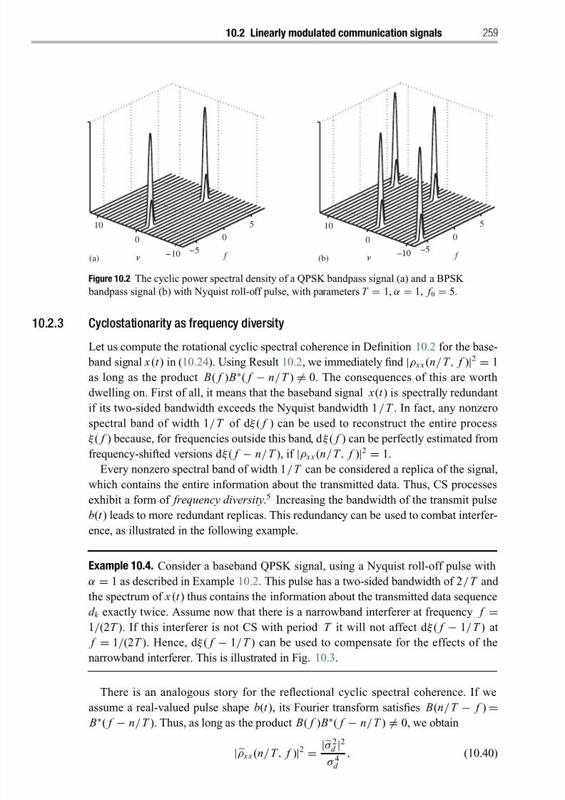
8/21/2019 Statistical Signal Processing of Complex-Valued Data.pdf
http://slidepdf.com/reader/full/statistical-signal-processing-of-complex-valued-datapdf 281/330
10.2 Linearly modulated communication signals 259
0
5
0
10
f ν
5
0
5
10
0
10
(a) (b) f ν
Figure 10.2 The cyclic power spectral density of a QPSK bandpass signal (a) and a BPSK bandpass signal (b) with Nyquist roll-off pulse, with parameters T = 1, α = 1, f 0 = 5.
10.2.3 Cyclostationarity as frequency diversity
Let us compute the rotational cyclic spectral coherence in Definition 10.2 for the base-
band signal x (t ) in (10.24). Using Result 10.2, we immediately find |ρ x x (n/ T , f )|2 = 1
as long as the product B( f ) B∗( f − n/ T ) = 0. The consequences of this are worth
dwelling on. First of all, it means that the baseband signal x(t ) is spectrally redundant
if its two-sided bandwidth exceeds the Nyquist bandwidth 1/ T . In fact, any nonzero
spectral band of width 1/ T of d ξ ( f ) can be used to reconstruct the entire processξ ( f ) because, for frequencies outside this band, d ξ ( f ) can be perfectly estimated from
frequency-shifted versions d ξ ( f − n/ T ), if |ρ x x (n/ T , f )|2 = 1.
Every nonzero spectral band of width 1/ T can be considered a replica of the signal,
which contains the entire information about the transmitted data. Thus, CS processes
exhibit a form of frequency diversity.5 Increasing the bandwidth of the transmit pulse
b(t ) leads to more redundant replicas. This redundancy can be used to combat interfer-
ence, as illustrated in the following example.
Example 10.4. Consider a baseband QPSK signal, using a Nyquist roll-off pulse with
α = 1 as described in Example 10.2. This pulse has a two-sided bandwidth of 2/ T and
the spectrum of x (t ) thus contains the information about the transmitted data sequence
d k exactly twice. Assume now that there is a narrowband interferer at frequency f =1/(2T ). If this interferer is not CS with period T it will not affect d ξ ( f − 1/ T ) at
f = 1/(2T ). Hence, d ξ ( f − 1/ T ) can be used to compensate for the effects of the
narrowband interferer. This is illustrated in Fig. 10.3.
There is an analogous story for the reflectional cyclic spectral coherence. If we
assume a real-valued pulse shape b(t ), its Fourier transform satisfies B(n/ T − f ) = B∗( f − n/ T ). Thus, as long as the product B( f ) B∗( f − n/ T ) = 0, we obtain
|ρ x x (n/ T , f )|2 = |σ 2d |2σ 4d
, (10.40)
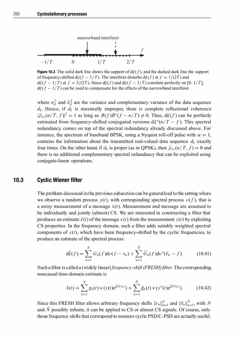
8/21/2019 Statistical Signal Processing of Complex-Valued Data.pdf
http://slidepdf.com/reader/full/statistical-signal-processing-of-complex-valued-datapdf 282/330
260 Cyclostationary processes
narrowband interferer
f
2 T 0 1 T −1 T
Figure 10.3 The solid dark line shows the support of d ξ ( f ), and the dashed dark line the support
of frequency-shifted d ξ ( f − 1/ T ). The interferer disturbs d ξ ( f ) at f = 1/(2T ) and
d ξ ( f − 1/ T ) at f = 3/(2T ). Since d ξ ( f ) and d ξ ( f − 1/ T ) correlate perfectly on [0, 1/ T ],
d ξ ( f − 1/ T ) can be used to compensate for the effects of the narrowband interferer.
where σ 2d and σ 2d are the variance and complementary variance of the data sequence
d k . Hence, if d k is maximally improper, there is complete reflectional coherence
|ρ x x (n/ T , f )|2
=1 as long as B( f ) B∗( f
−n/ T )
=0. Thus, d ξ ( f ) can be perfectly
estimated from frequency-shifted conjugated versions d ξ ∗(n/ T − f ). This spectral
redundancy comes on top of the spectral redundancy already discussed above. For
instance, the spectrum of baseband BPSK, using a Nyquist roll-off pulse with α = 1,
contains the information about the transmitted real-valued data sequence d k exactly
four times. On the other hand, if d k is proper (as in QPSK), then ρ x x (n/ T , f ) = 0 and
there is no additional complementary spectral redundancy that can be exploited using
conjugate-linear operations.
10.3 Cyclic Wiener filter
The problem discussed in the previous subsection can be generalized to the setting where
we observe a random process y(t ), with corresponding spectral process υ( f ), that is
a noisy measurement of a message x(t ). Measurement and message are assumed to
be individually and jointly (almost) CS. We are interested in constructing a filter that
produces an estimate ˆ x(t ) of the message x (t ) from the measurement y(t ) by exploiting
CS properties. In the frequency domain, such a filter adds suitably weighted spectral
components of y(t ), which have been frequency-shifted by the cyclic frequencies, to
produce an estimate of the spectral process:
d ξ ( f ) = N
n=1
G n( f )d υ( f − νn) +˜ N
n=1
G n( f )d υ∗(νn − f ). (10.41)
Such a filter is called a (widely linear) frequency-shift (FRESH) filter . Thecorresponding
noncausal time-domain estimate is
ˆ x(t ) = N
n=1
g n(t ) ∗ ( y(t )e j2π νn t ) +˜ N
n=1
˜ g n(t ) ∗ ( y∗(t )e j2π νn t ). (10.42)
Since this FRESH filter allows arbitrary frequency shifts {νn} N n=1 and {νn} ˜ N
n=1, with N
and ˜ N possibly infinite, it can be applied to CS or almost CS signals. Of course, only
those frequency shifts that correspond to nonzero cyclic PSD/C-PSD are actually useful.
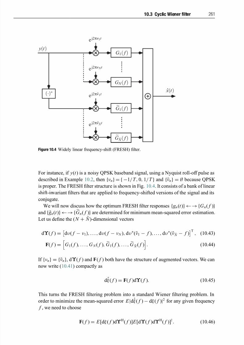
8/21/2019 Statistical Signal Processing of Complex-Valued Data.pdf
http://slidepdf.com/reader/full/statistical-signal-processing-of-complex-valued-datapdf 283/330
10.3 Cyclic Wiener filter 261
y(t )
e j2π ˜ ν ˜ N t
e j2π ˜ ν1t
G 1( f )
G ˜ N ( f )
G N ( f )
e j2π ν N t
G 1( f )
e j2π ν1t
(·)∗ ˆ x(t )
Figure 10.4 Widely linear frequency-shift (FRESH) filter.
For instance, if y(t ) is a noisy QPSK baseband signal, using a Nyquist roll-off pulse as
described in Example 10.2, then {νn} = { −1/ T , 0, 1/ T } and {νn} = ∅ because QPSK is proper. The FRESH filter structure is shown in Fig. 10.4. It consists of a bank of linear
shift-invariant filters that are applied to frequency-shifted versions of the signal and its
conjugate.
We will now discuss how the optimum FRESH filter responses { g n(t )}←→{G n( f )}and { ˜ g n(t )}←→{ G n( f )} are determined for minimum mean-squared error estimation.
Let us define the ( N + ˜ N )-dimensional vectors
d Υ( f ) =
d υ( f − ν1), . . . , d υ( f − ν N ), d υ∗(ν1 − f ), . . . , d υ∗(ν ˜ N − f )
T
, (10.43)
F( f ) = G 1( f ), . . . , G N ( f ), G 1( f ), . . . , G ˜ N ( f ). (10.44)
If {νn} = {νn}, d Υ( f ) and F( f ) both have the structure of augmented vectors. We can
now write (10.41) compactly as
d ξ ( f ) = F( f )d Υ( f ). (10.45)
This turns the FRESH filtering problem into a standard Wiener filtering problem. In
order to minimize the mean-squared error E |d ξ ( f )− d ξ ( f )|2
for any given frequency f , we need to choose
F( f ) = E [d ξ ( f )d ΥH( f )] E [d Υ( f )d ΥH( f )]†. (10.46)
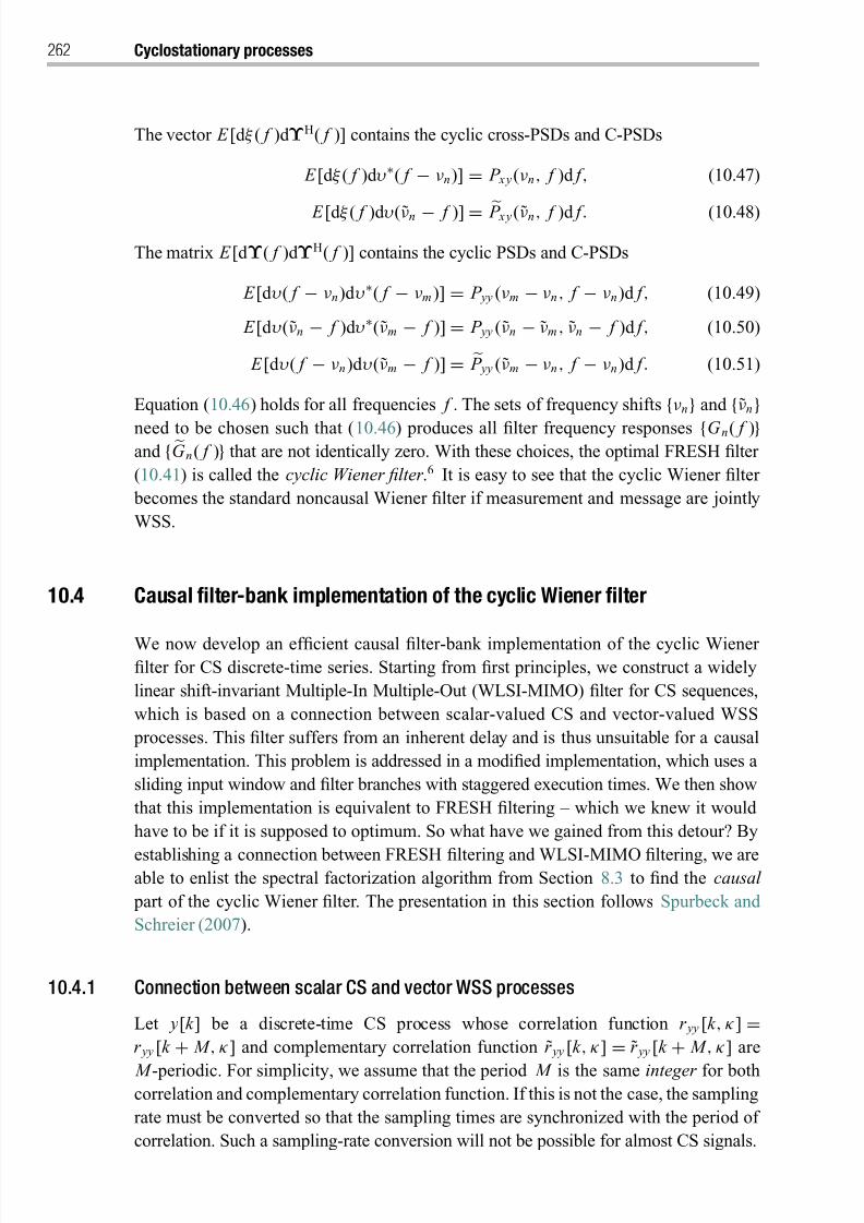
8/21/2019 Statistical Signal Processing of Complex-Valued Data.pdf
http://slidepdf.com/reader/full/statistical-signal-processing-of-complex-valued-datapdf 284/330
262 Cyclostationary processes
The vector E [d ξ ( f )d ΥH( f )] contains the cyclic cross-PSDs and C-PSDs
E [d ξ ( f )d υ∗( f − νn)] = P x y(νn, f )d f , (10.47)
E [d ξ ( f )d υ(νn − f )] = P x y(νn, f )d f . (10.48)
The matrix E [d Υ( f )d ΥH( f )] contains the cyclic PSDs and C-PSDs
E [d υ( f − νn)d υ∗( f − νm)] = P yy (νm − νn , f − νn)d f , (10.49)
E [d υ(νn − f )d υ∗(νm − f )] = P yy (νn − νm , νn − f )d f , (10.50)
E [d υ( f − νn)d υ(νm − f )] = P yy (νm − νn , f − νn)d f . (10.51)
Equation (10.46) holds for all frequencies f . The sets of frequency shifts {νn} and {νn}need to be chosen such that (10.46) produces all filter frequency responses {G n( f )}and { G n( f )} that are not identically zero. With these choices, the optimal FRESH filter
(10.41) is called the cyclic Wiener filter .6 It is easy to see that the cyclic Wiener filter
becomes the standard noncausal Wiener filter if measurement and message are jointly
WSS.
10.4 Causal filter-bank implementation of the cyclic Wiener filter
We now develop an efficient causal filter-bank implementation of the cyclic Wiener filter for CS discrete-time series. Starting from first principles, we construct a widely
linear shift-invariant Multiple-In Multiple-Out (WLSI-MIMO) filter for CS sequences,
which is based on a connection between scalar-valued CS and vector-valued WSS
processes. This filter suffers from an inherent delay and is thus unsuitable for a causal
implementation. This problem is addressed in a modified implementation, which uses a
sliding input window and filter branches with staggered execution times. We then show
that this implementation is equivalent to FRESH filtering – which we knew it would
have to be if it is supposed to optimum. So what have we gained from this detour? By
establishing a connection between FRESH filtering and WLSI-MIMO filtering, we areable to enlist the spectral factorization algorithm from Section 8.3 to find the causal
part of the cyclic Wiener filter. The presentation in this section follows Spurbeck and
Schreier (2007).
10.4.1 Connection between scalar CS and vector WSS processes
Let y[k ] be a discrete-time CS process whose correlation function r yy [k , κ] =r yy [k + M , κ] and complementary correlation function r yy [k , κ] = r yy [k + M , κ] are
M -periodic. For simplicity, we assume that the period M is the same integer for bothcorrelation and complementary correlation function. If this is not the case, the sampling
rate must be converted so that the sampling times are synchronized with the period of
correlation. Such a sampling-rate conversion will not be possible for almost CS signals.
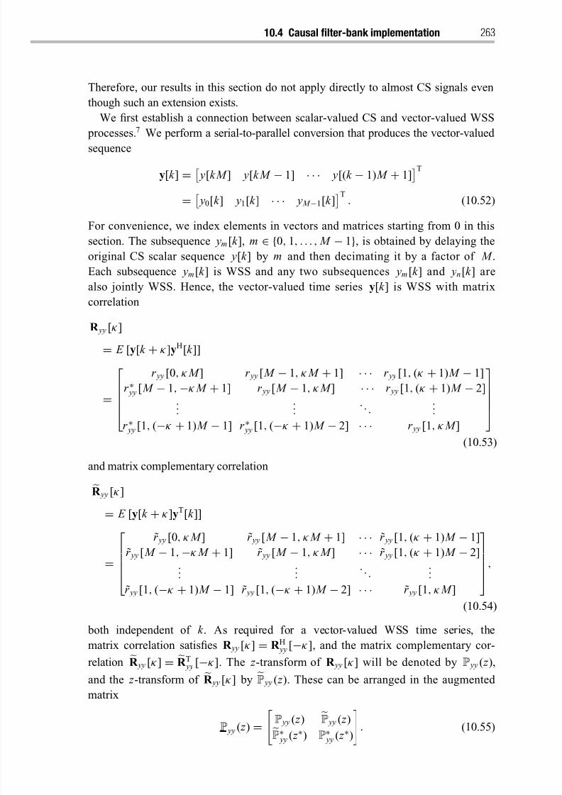
8/21/2019 Statistical Signal Processing of Complex-Valued Data.pdf
http://slidepdf.com/reader/full/statistical-signal-processing-of-complex-valued-datapdf 285/330
10.4 Causal filter-bank implementation 263
Therefore, our results in this section do not apply directly to almost CS signals even
though such an extension exists.
We first establish a connection between scalar-valued CS and vector-valued WSS
processes.7 We perform a serial-to-parallel conversion that produces the vector-valued
sequence
y[k ] = y[k M ] y[k M − 1] · · · y[(k − 1) M + 1]T
= y0[k ] y1[k ] · · · y M −1[k ]T
. (10.52)
For convenience, we index elements in vectors and matrices starting from 0 in this
section. The subsequence ym[k ], m ∈ {0, 1, . . . , M − 1}, is obtained by delaying the
original CS scalar sequence y[k ] by m and then decimating it by a factor of M .
Each subsequence ym
[k ] is WSS and any two subsequences ym
[k ] and yn[k ] are
also jointly WSS. Hence, the vector-valued time series y[k ] is WSS with matrix
correlation
R yy [κ]
= E [y[k + κ]yH[k ]]
=
r yy [0, κ M ] r yy [ M − 1, κ M + 1] · · · r yy [1, (κ + 1) M − 1]
r ∗ yy [ M − 1,−κ M + 1] r yy [ M − 1, κ M ] · · · r yy [1, (κ + 1) M − 2]...
... . . .
...
r ∗ yy [1, (−κ + 1) M − 1] r ∗ yy [1, (−κ + 1) M − 2] · · · r yy [1, κ M ]
(10.53)
and matrix complementary correlation
R yy [κ]
= E [y[k + κ]yT[k ]]
= r yy [0, κ M ] r yy [ M − 1, κ M + 1] · · · r yy [1, (κ + 1) M − 1]
r yy [ M − 1,−κ M + 1] r yy [ M − 1, κ M ] · · · r yy [1, (κ + 1) M − 2]......
. . . ...
r yy [1, (−κ + 1) M − 1] r yy [1, (−κ + 1) M − 2] · · · r yy [1, κ M ]
,
(10.54)
both independent of k . As required for a vector-valued WSS time series, the
matrix correlation satisfies R yy [κ] = R H yy [−κ], and the matrix complementary cor-
relation
R yy [κ] =
R T yy [−κ]. The z -transform of R yy [κ] will be denoted by P yy ( z ),
and the z -transform of
R yy [κ] by
P yy ( z ). These can be arranged in the augmented
matrix
P yy ( z ) =P yy ( z ) P yy ( z )P∗ yy ( z ∗) P∗ yy ( z ∗)
. (10.55)
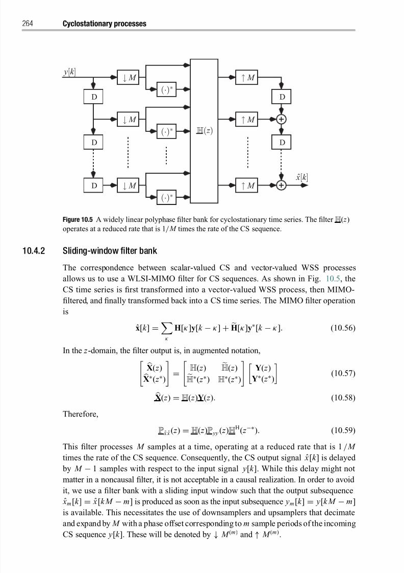
8/21/2019 Statistical Signal Processing of Complex-Valued Data.pdf
http://slidepdf.com/reader/full/statistical-signal-processing-of-complex-valued-datapdf 286/330
264 Cyclostationary processes
D
D
D
D
D
↑ M
↓ M
(·)∗
(·)∗↓ M
ˆ x[k ]
y[k ]
H( z )
↓ M
(
·)∗
↑ M
↑ M
Figure 10.5 A widely linear polyphase filter bank for cyclostationary time series. The filter H( z )
operates at a reduced rate that is 1/ M times the rate of the CS sequence.
10.4.2 Sliding-window filter bank
The correspondence between scalar-valued CS and vector-valued WSS processes
allows us to use a WLSI-MIMO filter for CS sequences. As shown in Fig. 10.5, the
CS time series is first transformed into a vector-valued WSS process, then MIMO-
filtered, and finally transformed back into a CS time series. The MIMO filter operationis
x[k ] =
κ
H[κ]y[k − κ] + H[κ]y∗[k − κ]. (10.56)
In the z -domain, the filter output is, in augmented notation, X( z )
X∗( z ∗)
= H( z ) H( z )
H∗( z ∗) H∗( z ∗)
Y( z )
Y∗( z ∗)
(10.57)
X( z ) = H( z )Y( z ). (10.58)Therefore,
P ˆ x ˆ x ( z ) = H( z )P yy ( z )HH( z −∗). (10.59)
This filter processes M samples at a time, operating at a reduced rate that is 1/ M
times the rate of the CS sequence. Consequently, the CS output signal ˆ x[k ] is delayed
by M − 1 samples with respect to the input signal y[k ]. While this delay might not
matter in a noncausal filter, it is not acceptable in a causal realization. In order to avoid
it, we use a filter bank with a sliding input window such that the output subsequence
ˆ xm[k ] = ˆ x[k M − m] is produced as soon as the input subsequence ym[k ] = y[k M − m]is available. This necessitates the use of downsamplers and upsamplers that decimate
and expand by M with a phase offset corresponding to m sample periods of the incoming
CS sequence y[k ]. These will be denoted by ↓ M (m) and ↑ M (m).
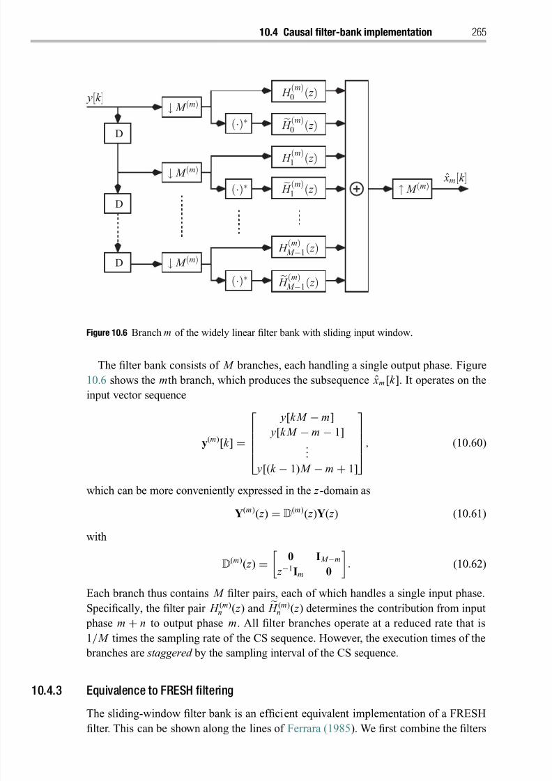
8/21/2019 Statistical Signal Processing of Complex-Valued Data.pdf
http://slidepdf.com/reader/full/statistical-signal-processing-of-complex-valued-datapdf 287/330
10.4 Causal filter-bank implementation 265
D
D
D
(
·)∗
↓ M (m)
↑ M (m)
↓ M (m)
↓ M (m)
H (m)
M −1( z )
H (m)
M −1( z )
H (m)1 ( z )
H (m)1 ( z )
H (m)0 ( z )
H (m)0 ( z )
ˆ xm[k ]
y[k ]
(·)∗
(·)∗
Figure 10.6 Branch m of the widely linear filter bank with sliding input window.
The filter bank consists of M branches, each handling a single output phase. Figure
10.6 shows the mth branch, which produces the subsequence ˆ xm[k ]. It operates on the
input vector sequence
y(m)[k ] =
y[k M − m]
y[k M − m − 1]...
y[(k − 1) M − m + 1]
, (10.60)
which can be more conveniently expressed in the z -domain as
Y(m)( z ) = D(m)( z )Y( z ) (10.61)
with
D(m)( z ) = 0 I M −m
z −1Im 0
. (10.62)
Each branch thus contains M filter pairs, each of which handles a single input phase.
Specifically, the filter pair H (m)n ( z ) and H (m)
n ( z ) determines the contribution from input
phase m + n to output phase m. All filter branches operate at a reduced rate that is
1/ M times the sampling rate of the CS sequence. However, the execution times of the
branches are staggered by the sampling interval of the CS sequence.
10.4.3 Equivalence to FRESH filtering
The sliding-window filter bank is an efficient equivalent implementation of a FRESH
filter. This can be shown along the lines of Ferrara (1985). We first combine the filters
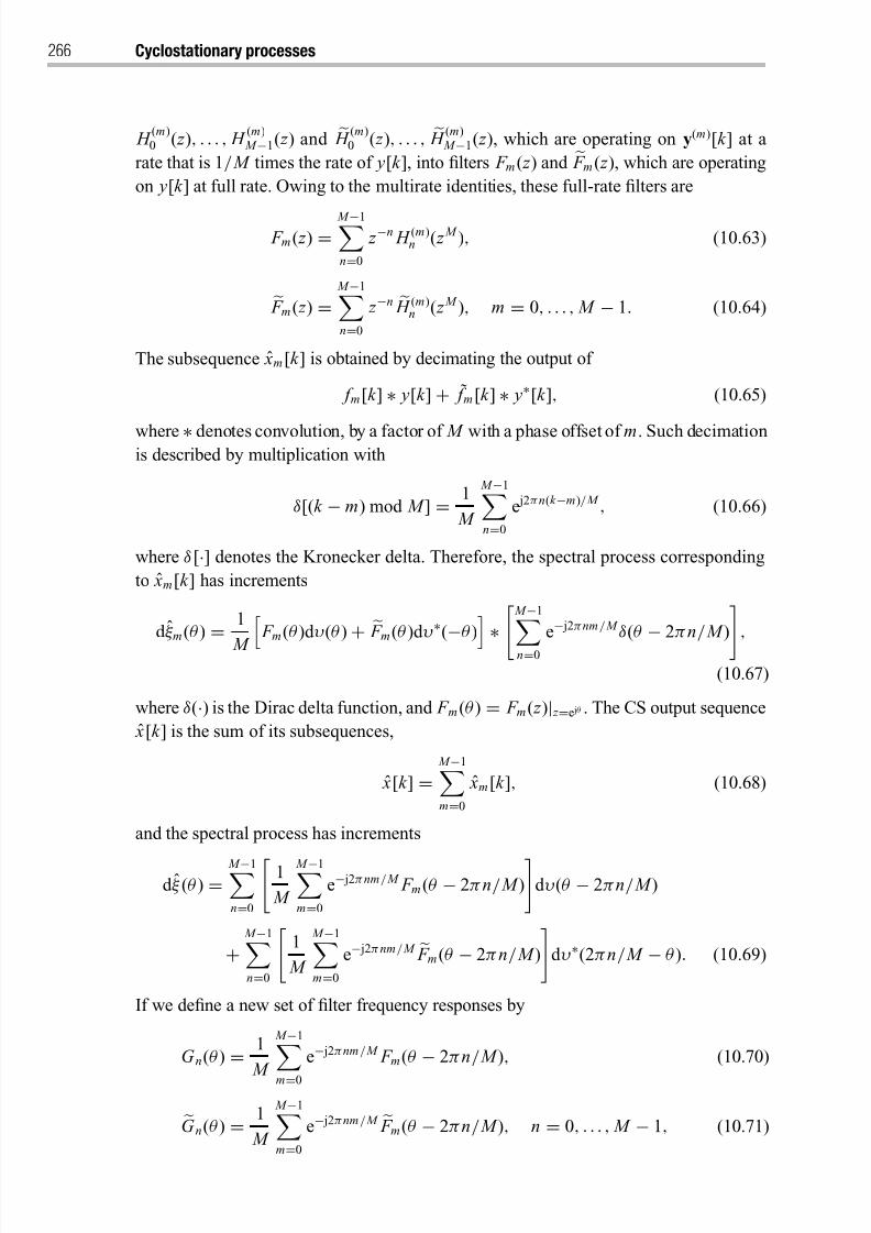
8/21/2019 Statistical Signal Processing of Complex-Valued Data.pdf
http://slidepdf.com/reader/full/statistical-signal-processing-of-complex-valued-datapdf 288/330
266 Cyclostationary processes
H (m)0 ( z ), . . . , H
(m) M −1( z ) and H
(m)0 ( z ), . . . , H
(m) M −1( z ), which are operating on y(m)[k ] at a
rate that is 1/ M times the rate of y[k ], into filters F m( z ) and
F m( z ), which are operating
on y[k ] at full rate. Owing to the multirate identities, these full-rate filters are
F m( z ) = M −1n=0
z −n H (m)n ( z M ), (10.63)
F m( z ) = M −1n=0
z −n H (m)n ( z M ), m = 0, . . . , M − 1. (10.64)
The subsequence ˆ xm[k ] is obtained by decimating the output of
f m[k ] ∗ y[k ] + ˜ f m[k ] ∗ y∗[k ], (10.65)
where ∗ denotes convolution, by a factor of M with a phase offset of m. Such decimationis described by multiplication with
δ[(k − m) mod M ] = 1
M
M −1n=0
e j2π n(k −m)/ M , (10.66)
where δ[·] denotes the Kronecker delta. Therefore, the spectral process corresponding
to ˆ xm[k ] has increments
d ξ m(θ )
=1
M F m(θ )d υ(θ )
+ F m(θ )d υ∗(
−θ ) ∗
M −1
n=0
e− j2π nm / M δ(θ
−2π n/ M ),
(10.67)
where δ(·) is the Dirac delta function, and F m(θ ) = F m( z )| z =e jθ . The CS output sequence
ˆ x[k ] is the sum of its subsequences,
ˆ x[k ] = M −1m=0
ˆ xm[k ], (10.68)
and the spectral process has increments
d ξ (θ ) = M −1n=0
1
M
M −1m=0
e− j2π nm/ M F m(θ − 2π n/ M )
d υ(θ − 2π n/ M )
+ M −1n=0
1
M
M −1m=0
e− j2π nm/ M F m(θ − 2π n/ M )
d υ∗(2π n/ M − θ ). (10.69)
If we define a new set of filter frequency responses by
G n(θ ) = 1
M
M −1
m=0
e− j2π nm / M F m(θ − 2π n/ M ), (10.70)
G n(θ ) = 1
M
M −1m=0
e− j2π nm / M F m(θ − 2π n/ M ), n = 0, . . . , M − 1, (10.71)
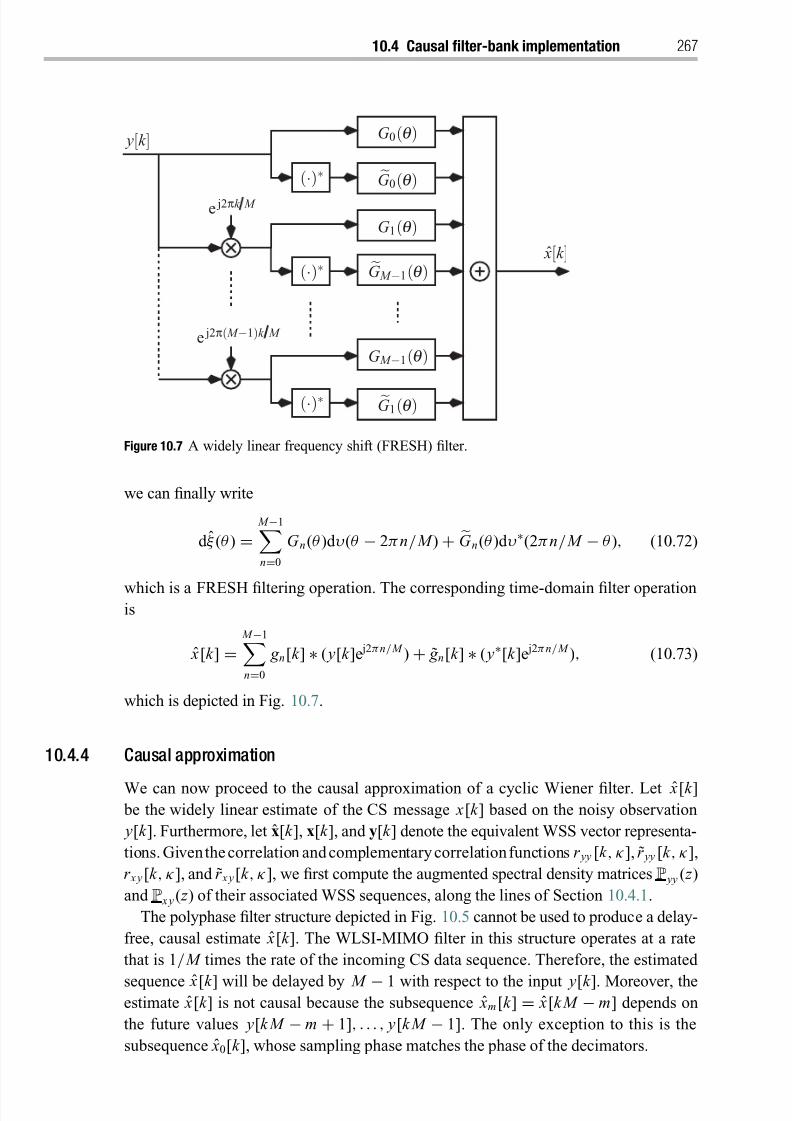
8/21/2019 Statistical Signal Processing of Complex-Valued Data.pdf
http://slidepdf.com/reader/full/statistical-signal-processing-of-complex-valued-datapdf 289/330
10.4 Causal filter-bank implementation 267
e j2π( M −1)k M
G 1(q)
G M −1(q)
G M −1(q)
G 1(q)
G 0(q)
ˆ x[k ]
y[k ] G 0(q)
(
·)∗
(·)∗
(·)∗
e j2πk M
Figure 10.7 A widely linear frequency shift (FRESH) filter.
we can finally write
d ξ (θ ) = M −1n=0
G n(θ )d υ(θ − 2π n/ M ) +
G n(θ )d υ∗(2π n/ M − θ ), (10.72)
which is a FRESH filtering operation. The corresponding time-domain filter operationis
ˆ x[k ] = M −1n=0
g n[k ] ∗ ( y[k ]e j2π n/ M ) + ˜ g n[k ] ∗ ( y∗[k ]e j2π n/ M ), (10.73)
which is depicted in Fig. 10.7.
10.4.4 Causal approximation
We can now proceed to the causal approximation of a cyclic Wiener filter. Let ˆ x[k ] be the widely linear estimate of the CS message x[k ] based on the noisy observation
y[k ]. Furthermore, let x[k ], x[k ], and y[k ] denote the equivalent WSS vector representa-
tions. Giventhecorrelation and complementary correlationfunctions r yy [k , κ], r yy [k , κ],
r x y[k , κ], and r x y[k , κ], we first compute the augmented spectral density matrices P yy ( z )
and P x y( z ) of their associated WSS sequences, along the lines of Section 10.4.1.
The polyphase filter structure depicted in Fig. 10.5 cannot be used to produce a delay-
free, causal estimate ˆ x[k ]. The WLSI-MIMO filter in this structure operates at a rate
that is 1/ M times the rate of the incoming CS data sequence. Therefore, the estimated
sequence ˆ x[k ] will be delayed by M − 1 with respect to the input y[k ]. Moreover, theestimate ˆ x[k ] is not causal because the subsequence ˆ xm[k ] = ˆ x[k M − m] depends on
the future values y[k M − m + 1], . . . , y[k M − 1]. The only exception to this is the
subsequence ˆ x0[k ], whose sampling phase matches the phase of the decimators.

8/21/2019 Statistical Signal Processing of Complex-Valued Data.pdf
http://slidepdf.com/reader/full/statistical-signal-processing-of-complex-valued-datapdf 290/330
268 Cyclostationary processes
To circumvent this problem, we use the filter bank with sliding input window whose
mth branch is shown in Fig. 10.6. The subsequence estimate ˆ xm[k ] is based on the
vector sequence y(m)[k ] with a phase offset of m samples relative to y[k ], as defined
in (10.60)–(10.62). The vector sequence y(m)[k ] is still WSS with augmented spectral
density matrix
P(m) yy ( z ) =
D(m)( z ) 0
0 D(m)( z )
P yy ( z )
D(m)( z −1) 0
0 D(m)( z −1)
T
. (10.74)
We may now utilize our results from Section 8.3 to spectrally factor
P(m) yy ( z ) = A(m)
yy ( z )(A(m) yy )H( z −∗), (10.75)
where A(m) yy ( z ) is minimum phase, meaning that both A(m)
yy ( z ) and its inverse are causal
and stable. The cross-spectral density matrix P(m) x y ( z ) is found analogously to (10.74),
P(m) x y ( z ) =
D(m)( z ) 0
0 D(m)( z )
P x y( z )
D(m)( z −1) 0
0 D(m)( z −1)
T
. (10.76)
The transfer function of a causal WLMMSE filter for the augmented WSS vector
sequence y(m)[k ] can now be obtained as
H(m)( z ) = [P(m) x y ( z )(A(m)
yy )−H( z −∗)]+(A(m) yy )−1( z ), (10.77)
where [·]+ denotes the causal part. Again, only the subsequence ˆ xm[k ] produced by thisfilter is a delay-free, causal MMSE estimate. Hence, for each polyphase matrixH(m)( z ),
we extract the top row vector, denoted by H
(m)0 ( z ) · · · H
(m) M −1( z ) H
(m)0 ( z ) · · · H
(m) M −1( z )
. (10.78)
This vector is the polyphase representation of a causal WLMMSE filter that produces
the mth subsequence ˆ xm[k ] of the CSestimate ˆ x[k ]. This filter constitutes the mth branch
shown in Fig. 10.6. The causal widely linear MMSE filter for producing ˆ x[k ] from y[k ]
comprises a parallel collection of M such filters, whose outputs are summed.
Notes
1 CS processes for which ensemble averages can be replaced by time averages are sometimes
called cycloergodic. An in-depth treatmentof cycloergodicity is provided byBoylesand Gardner
(1983). Gardner (1988) presents a treatment of cyclostationary processes in the fraction-of-time
probabilistic framework, which is entirely based on time averages.
2 A thorough discussion of estimators for the cyclic correlation and PSD, including the proof that
the time-smoothed and frequency-smoothed cyclic periodograms are asymptotically equivalent,
is provided by Gardner (1986).
3 The cyclic PSDs of several digital communication signals were derived by Gardner et al . (1987).
A closer look at the cyclic PSD of continuous-phase modulated (CPM) signals is provided by
Napolitano and Spooner (2001).

8/21/2019 Statistical Signal Processing of Complex-Valued Data.pdf
http://slidepdf.com/reader/full/statistical-signal-processing-of-complex-valued-datapdf 291/330
Notes 269
4 Improper digital communication signals include all real-valued baseband signals such as Pulse
Amplitude Modulation (PAM) and Binary Phase Shift Keying (BPSK), but also Offset Quater-
nary Phase Shift Keying (OQPSK), Minimum Shift Keying (MSK), and Gaussian Minimum
Shift Keying (GMSK). GMSK is used in the mobile-phone standard GSM.
5 The term “diversity” is commonly used in mobile communications, where the receiver obtainsseveral replicas of the same information-bearing signal. In “frequency diversity,” the signal is
transmitted on several carriers that are sufficiently separated in frequency.
6 FRESH filtering and the cyclic Wiener filter were introduced and analyzed by Gardner (1988,
1993). The cyclic Wiener filter utilizes the frequency diversity of CS signals in a way that
is reminiscent of the RAKE receiver in wireless communications (see Proakis (2001) for
background on the RAKE receiver).
7 The connection between scalar-valued CS and vector-valued WSS time series was found by
Gladyshev (1961). There is a corresponding result for continuous-time CS processes due to
Gladyshev (1963). If x (t ) is CS with period T , and θ an independent random variable uniformly
distributed over [0, T ], then xm (t )
= x (t
−θ )e j2π m(t −θ )/T is WSS, and xm (t ) and xn(t ) are jointly
WSS.
8/21/2019 Statistical Signal Processing of Complex-Valued Data.pdf
http://slidepdf.com/reader/full/statistical-signal-processing-of-complex-valued-datapdf 292/330
Appendix 1Rudiments of matrix analysis
In this appendix, we present a very concise review of some basic results in matrix
analysis that are used in this book. As an excellent reference for further reading we
recommend Horn and Johnson (1985).
A1.1 Matrix factorizations
A1.1.1 Partitioned matrices
If A and D are square matrices and have inverses, there exist the factorizations
A =
A B
C D=
I BD−1
0 I A − BD−1C 0
0 D I 0
D−1C I (A1.1)
=
I 0
CA−1 I
A 0
0 D − CA−1B
I A−1B
0 I
(A1.2)
The factors A − BD−1C and D − CA−1B are referred to as the Schur complements
of D and A, respectively, within A. These factorizations establish the determinant
formulae
detA = det(A − BD−1C)det D (A1.3)
=det A det(D
−CA−1B). (A1.4)
A1.1.2 Eigenvalue decomposition
A matrix A ∈ Cn×n is normal if it commutes with itsHermitian transpose: AAH = AHA.
A matrix is Hermitian if it is Hermitian-symmetric: AH = A. Any Hermitian matrix is
therefore normal.
Every normal matrix has the factorization
A = UΛUH, (A1.5)
calledan eigenvalue (or spectral) decomposition(EVD), where U is unitary. Thecolumnsui of U are called the eigenvectors, and the diagonal matrix Λ = Diag(λ1, λ2, . . . , λn)
contains the eigenvalueson its diagonal. We will assumethe ordering |λ1| ≥ |λ2| ≥ · · · ≥|λn|. The number r of nonzero eigenvalues is the rank of A, and the zero eigenvalues are
8/21/2019 Statistical Signal Processing of Complex-Valued Data.pdf
http://slidepdf.com/reader/full/statistical-signal-processing-of-complex-valued-datapdf 293/330
Rudiments of matrix analysis 271
λr +1 = λr +2 = · · · = λn = 0. Thus, A may be expressed as
A =r
i=1
λi ui uHi , (A1.6)
and, for any polynomial f ,
f (A) =r
i=1
f (λi )ui uHi . (A1.7)
An important fact is that the nonzero eigenvalues of a product of matrices AB are the
nonzero eigenvalues of BA, for arbitrary A and B.
The following list contains equivalent statements for different types of normal matri-
ces.
A = AH ⇔ λi real for all i, (A1.8)
A unitary ⇔ |λi | = 1 for all i, (A1.9)
A positive definite ⇔ λi > 0 for all i, (A1.10)
A positive semidefinite ⇔ λi ≥ 0 for all i. (A1.11)
2 × 2 matrix
The two eigenvalues of the 2 × 2 matrix
A = a b
c d (A1.12)
are
λ1,2 = 12 tr A ± 1
2
tr 2A − 4det A (A1.13)
and the unit-length eigenvectors are
u1 =1
u1
b
λ1 − a
, (A1.14)
u2 =1
u2 b
λ2 − a . (A1.15)
A1.1.3 Singular value decomposition
Every matrix A ∈ Cn×m has the factorization
A = FKGH, (A1.16)
called a singular value decomposition (SVD), where F ∈ Cn× p and G ∈ Cm× p, p =min(n, m), both have unitary columns, FHF = I and GHG = I. The columns f i of F are
called the left singular vectors, and the columns gi of G are called the right singular vectors. The diagonal matrix K = Diag(k 1, k 2, . . . , k p) contains the singular values
k 1 ≥ k 2 ≥ · · · ≥ k p ≥ 0 on its diagonal. The number r of nonzero singular values is the
rank of A.
8/21/2019 Statistical Signal Processing of Complex-Valued Data.pdf
http://slidepdf.com/reader/full/statistical-signal-processing-of-complex-valued-datapdf 294/330
272 Appendix 1
Since AAH = FKGH(GKFH) = FK 2FH and AHA = (GKFH)FKGH = GK 2GH, the
singular values of A are the nonnegative roots of the eigenvalues of AAH or
AHA. So, for normal A, how are the EVD A = UΛUH and the SVD A =
FKG
H
related? If we write Λ
= |Λ|D with |
Λ| = Diag(|λ1|, |λ2|, . . . , |λn|) and D =Diag(exp(jλ1), exp(jλ2), . . . , exp(jλn)) then
A = UΛUH = U|Λ|(UDH)H = FKGH (A1.17)
is an SVD of A with F = U, K = |Λ|, and G = UD∗. Therefore, the singular values of
A are the absolute values of the eigenvalues of A. If A is Hermitian, then the eigenvalues
and thus D are real, and D = Diag(sign(λ1), sign(λ2), . . . , sign(λn)). If A is Hermitian
and positive semidefinite, then F = G = U and K = Λ. That is, the SVD and EVD of
a Hermitian positive semidefinite matrix are identical.
A1.2 Positive definite matrices
Positive definite and semidefinite matrices are important because correlation and covari-
ance matricesarepositive(semi)definite.A Hermitian matrix A ∈ Cn×n is called positive
definite if
xHAx > 0 for all nonzero x ∈ Cn (A1.18)
and positive semidefinite if the weaker condition xHAx
≥0 holds. A Hermitian matrix is
positive definite if and only if all of its eigenvalues are positive, and positive semidefiniteif and only if all eigenvalues are nonnegative.
A1.2.1 Matrix square root and Cholesky decomposition
A matrix A is positive definite if and only if there exists a nonsingular lower-triangular
matrix L with positive diagonal entries such that A = LLH. This factorization is often
called the Cholesky decomposition of A. It determines a square root A1/2 = L, which is
neither positive definite nor Hermitian.
The unique positive semidefinite square root of a positive semidefinite matrix A isobtained via the EVD of A = UΛUH as
A1/2 = UΛ1/2UH (A1.19)
with Λ1/2 = Diag(√
λ1,√
λ2, . . . ,√
λn).
A1.2.2 Updating the Cholesky factors of a Grammian matrix
Consider the data matrix X p = [x1, x2, . . . , x p] ∈ Cn× p with n ≥ p and positive definite
Grammian matrix
G p = XH p X p =
G p−1 h p
hH p h pp
, (A1.20)
8/21/2019 Statistical Signal Processing of Complex-Valued Data.pdf
http://slidepdf.com/reader/full/statistical-signal-processing-of-complex-valued-datapdf 295/330
Rudiments of matrix analysis 273
where G p−1 = XH p−1X p−1, h p = XH
p−1x p and h pp = xH p x p. The Cholesky decomposi-
tion of G p−1 is G p−1 = L p−1LH p−1, where L p−1 is lower-triangular. It follows that the
Cholesky factors of G p may be updated as
G p = L pLH p = L p−1 0
mT p m pp
LH p−1 m∗ p0 m∗
pp
= G p−1 h p
hH p h pp
, (A1.21)
where m p and m pp solve the following consistency equations:
L p−1m∗ p = h p, (A1.22)
mT pm∗
p + |m pp |2 = h pp . (A1.23)
This factorization may then be inverted for G−1 p to achieve the upper-triangular–lower-
triangular factorization
G−1 p = L−H
p L−1 p =
L−H p−1 k p
0 k pp
L−1 p−1 0
k H p k ∗ pp
. (A1.24)
From the constraint that L−1 p L p = I, k p and k pp are determined from the consistency
equations
k H p L p−1 = −k ∗ pp mT p, (A1.25)
k ∗ pp m pp = 1. (A1.26)
A1.2.3 Partial ordering
For A, B ∈ Cn×n , we write A > B when A − B is positive definite, and A ≥ B when
A − B is positive semidefinite. This is a partial ordering of the set of n × n Hermitian
matrices. It is partial because we may have A B and B A. For A > 0, B ≥ 0, and
nonsingular C, we have
CHAC > 0, (A1.27)
CHBC
≥0, (A1.28)
A−1 > 0, (A1.29)
A + B ≥ A > 0, (A1.30)
A ≥ B ⇒ evi (A) ≥ evi (B). (A1.31)
The last statement assumes that the eigenvalues of A and B are each arranged in
decreasing order. As a particular consequence, det A ≥ det B and tr A ≥ tr B.
The partitioned Hermitian matrix
A = A B
BH D, (A1.32)
with square blocks A and D, is positive definite if and only if A > 0 and its Schur
complement D − BHA−1B > 0, or D > BHA−1B.
8/21/2019 Statistical Signal Processing of Complex-Valued Data.pdf
http://slidepdf.com/reader/full/statistical-signal-processing-of-complex-valued-datapdf 296/330
274 Appendix 1
A1.2.4 Inequalities
There are several important determinant inequalities, which can all be proved from
partial-ordering results. Alternative closely related proofs are also possible via majoriza-
tion, which is discussed in Appendix 3. The Hadamard determinant inequality for a positive semidefinite A ∈ Cn×n is
det A ≤n
i=1
Aii . (A1.33)
For positive definite A, equality holds if and only if A is diagonal.
The Fischer determinant inequality for the partitioned positive definite matrix A in
(A1.32) is
detA ≤ det A det D. (A1.34)
The Minkowski determinant inequality for positive definite A, B ∈ Cn×n is
det1/n(A + B) ≥ det1/n A + det1/n B, (A1.35)
with equality if and only if B = cA for some positive constant c.
A1.3 Matrix inverses
A1.3.1 Partitioned matrices
The inverse of a block-diagonal matrix of nonsingular blocks is obtained by taking the
inverses of the individual blocks,
[Diag(A1, A2, . . . , Ak )]−1 = Diag(A−1
1 , A−12 , . . . , A−1
k ). (A1.36)
Given the factorizations (A1.1) and (A1.2) for the partitioned matrix A and the
identities
I X
0 I −1
= I −
X
0 I and I 0
X I−1
= I 0
−X I (A1.37)
there are the following corresponding factorizations for A−1:
A−1=
A B
C D
−1
=
I 0
−D−1C I
(A − BD−1C)−1 0
0 D−1
I −BD−1
0 I
(A1.38)
=
I −A−1B
0 I
A−1 0
0 (D − CA−1B)−1
I 0
−CA−1 I
. (A1.39)
These lead to the determinant formulaedetA−1 = det(A − BD−1C)−1 det D−1 (A1.40)
= det A−1 det(D − CA−1B)−1 (A1.41)

8/21/2019 Statistical Signal Processing of Complex-Valued Data.pdf
http://slidepdf.com/reader/full/statistical-signal-processing-of-complex-valued-datapdf 297/330
Rudiments of matrix analysis 275
and a formula for A−1, which is sometimes called the matrix-inversion lemma:
A−1 =
A B
C D−1
=
(A − BD−1C)−1 −(A − BD−1C)−1BD−1
−(D
−CA−1B)−1CA−1 (D
−CA−1B)−1
. (A1.42)
Different expressions may be derived by employing the Woodbury identities
(A − BD−1C)−1 = A−1 + A−1B(D − CA−1B)−1CA−1, (A1.43)
(A − BD−1C)−1BD−1 = A−1B(D − CA−1B)−1. (A1.44)
A simple special case is the inverse of a 2 × 2 matrixa b
c d
−1
= 1
ad − bc
d −b
−c a
. (A1.45)
A1.3.2 Moore–Penrose pseudo-inverse
Let A ∈ Cn×m , possibly rank-deficient. Its Moore–Penrose pseudo-inverse (or general-
ized inverse) A† ∈ Cm×n satisfies the following conditions:
A†A = (A†A)H, (A1.46)
AA† = (AA†)H, (A1.47)
A†AA†
=A†, (A1.48)
AA†A = A. (A1.49)
The pseudo-inverse always exists and is unique. It may be computed via the SVD of A =FKGH, as A† = GK †FH. The pseudo-inverse of K = Diag(k 1, k 2, . . . , k r , 0, . . . , 0),
k r > 0, is K † = Diag(k −11 , k −1
2 , . . . , k −1r , 0, . . . , 0). The SVD is an expensive thing to
compute but the pseudo-inverse may be computed inexpensively via a Gram–Schmidt
factorization.
Example A1.1. If the 2 × 2 positive semidefinite Hermitian matrix
A =
a b
b∗ d
(A1.50)
is singular, i.e., ad = |b|2, then its eigen- and singular values are λ1 = a + d and λ2 = 0,
thanks to (A1.13). The eigen- and singular vector associated with λ1 is
u1 =1
u1
b
d
. (A1.51)
The pseudo-inverse of A is therefore
A† = λ−11 u1uH
1 =1
(a + d )(|b|2 + d 2)
|b|2 bd
b∗d d 2
. (A1.52)

8/21/2019 Statistical Signal Processing of Complex-Valued Data.pdf
http://slidepdf.com/reader/full/statistical-signal-processing-of-complex-valued-datapdf 298/330
276 Appendix 1
There are special cases when A has full rank. If m ≤ n, then A† = (AHA)−1AH, and
A†A = Im×m . If n ≤ m, then A† = AH(AAH)−1, and AA† = In×n. If A is square and
nonsingular, then A† = A−1.
A1.3.3 Projections
A matrix P ∈ Cn×n that satisfies P2 = P is called a projection. If, in addition, P = PH
then P isan orthogonal projection. For H ∈ Cn× p, the matrix PH = HH† is an orthogonal
projection whose range is the range of H. If H has full rank and p ≤ n, PH = HH† =H(HHH)−1HH. I f [H, A] is a full rank n × n matrix, where H ∈ Cn× p and A ∈ Cn×(n− p),
then
x = PHx + PAx (A1.53)
decomposes the vector x into two orthogonal components, one of which lies in H and
the other of which lies in A. Note that PA = A(AHA)−1AH = I − PH.
8/21/2019 Statistical Signal Processing of Complex-Valued Data.pdf
http://slidepdf.com/reader/full/statistical-signal-processing-of-complex-valued-datapdf 299/330
Appendix 2 Complex differentialcalculus (Wirtinger calculus)
In statistical signal processing, we often deal with a real nonnegative cost function, such
as a likelihood function or a quadratic form, which is then either analytically or numer-
ically optimized with respect to a vector or matrix of parameters. This involves taking
derivatives with respect to vectors or matrices, leading to gradient vectors and Jaco-
bian and Hessian matrices. What happens when the parameters are complex-valued?
That is, how do we differentiate a real-valued function with respect to a complex
argument?
What makes this situation confusing is that classical complex analysis tells us that a
complex function is differentiable on its entire domain if and only if it is holomorphic
(which is a synonym for complex analytic). A holomorphic function with nonzero
derivative is conformal because it preserves angles (including their orientations) and the
shapes of infinitesimally small figures (but not necessarily their size) in the complex
plane. Since nonconstant real-valued functions defined on the complex domain cannot
be holomorphic, their classical complex derivatives do not exist.
We can, of course, regard a function f defined on Cn as a function defined on IR 2n. If
f is differentiable on IR 2n , it is said to be real-differentiable, and if f is differentiable
on Cn , it is complex-differentiable. A function is complex-differentiable if and only
if it is real-differentiable and the Cauchy–Riemann equations hold. Is there a way to
define generalized complex derivatives for functions that are real-differentiable but not
complex-differentiable?Thiswouldextend complexdifferential calculus in a way similar
to the way that impropriety extends the theory of complex random variables.
It is indeed possible to do this. The theory was developed by the Austrian mathe-matician Wilhelm Wirtinger (1927), which is why this generalized complex differential
calculus is sometimes referred to as Wirtinger calculus. In the engineering literature,
Wirtinger calculus was rediscovered by Brandwood (1983) and then further developed
by van den Bos (1994a). In this appendix, we mainly follow the outline by van den Bos
(1994a), with some minor extensions.
The key idea of Wirtinger calculus is to formally regard f as a function of two
independent complex variables x and x∗. A generalized complex derivative is then
formally defined as the derivative with respect to x , while treating x∗ as a constant.
Another generalized derivative is defined as the derivative with respect to x∗, whileformally treating x as a constant. The generalized derivatives exist whenever f is real-
differentiable. These ideas extend in a straightforward fashion to complex gradients,
Jacobians, and Hessians.
8/21/2019 Statistical Signal Processing of Complex-Valued Data.pdf
http://slidepdf.com/reader/full/statistical-signal-processing-of-complex-valued-datapdf 300/330
278 Appendix 2
A2.1 Complex gradients
We shall begin with a scalar real-valued, totally differentiable function f (z), z =
[u, v]
T
∈ IR
2
. Its linear approximation at z0 = [u0, v0]
T
is
f (z) = f (u, v) ≈ f (z0) +∇ z f (z0)(z − z0), (A2.1)
with the gradient (a row vector)
∇ z f (z0) =
∂ f
∂u(z0)
∂ f
∂v(z0)
. (A2.2)
How should the approximation (A2.1) work for a real-valued function with complex
argument? Letting x = u + jv, we may express f as a function of complex x . In a slight
abuse of notation, we write f ( x) = f (z). Utilizing the 2 × 2 real-to-complex matrix
T =
1 j
1 − j
, (A2.3)
which satisfies THT = TTH = 2I, we now obtain
∇ z f (z0)(z − z0) = 12∇ z f (z0)TH
(T(z − z0)) (A2.4)
= ∇ x f ( x0)
x − x0
x∗
− x∗0
(A2.5)
= ∇ x f ( x0)(x − x0). (A2.6)
This introduces the augmented vector
x =
x
x∗
=
u + jv
u − jv
= Tz. (A2.7)
Using (A2.4) –(A2.6), we define the complex gradient
∇ x f ( x0) 1
2∇ z f (z
0)TH
= 1
2∂ f
∂u − j
∂ f
∂v(z
0)
1
2∂ f
∂u + j
∂ f
∂v(z
0). (A2.8)
In (A2.5), the first component of ∇ x f ( x0) operates on x and the second component
operates on x ∗. Thus,
∇ x f ( x0) =
∂ f
∂ x( x0)
∂ f
∂ x∗ ( x0)
. (A2.9)
By equating this expression with the right-hand side of (A2.8), we obtain the following
definition.
Definition A2.1. The generalized complex differential operator is defined as
∂
∂ x
1
2
∂
∂u− j
∂
∂v
(A2.10)

8/21/2019 Statistical Signal Processing of Complex-Valued Data.pdf
http://slidepdf.com/reader/full/statistical-signal-processing-of-complex-valued-datapdf 301/330
Complex differential calculus (Wirtinger calculus) 279
and the conjugate generalized complex differential operator as
∂
∂ x∗
1
2 ∂
∂u+ j
∂
∂v. (A2.11)
The derivatives obtained by applying the generalized complex and conjugate com-
plex differential operators are called Wirtinger derivatives after the pioneering work of
Wirtinger (1927). These generalized differential operators can be formally implemented
by treating x and x ∗ as independent variables. That is, when applying ∂/∂ x , we take the
derivative with respect to x while formally treating x∗ as a constant. Similarly, ∂/∂ x∗
yields the derivative with respect to x ∗, regarding x as a constant. The following example
shows how this approach works.
Example A2.1. Consider the function f ( x) = | x|2 = x x∗. Treating x and x∗ as two
independent variables, we find
∂ f ( x)
∂ x= x∗ and
∂ f ( x)
∂ x∗ = x .
This can be checked by writing f ( x) = f (u, v) = u2 + v2 and
1
2 ∂
∂u− j
∂
∂v f (u, v) = u − jv = x∗,
1
2
∂
∂u+ j
∂
∂v
f (u, v) = u + jv = x .
The linear approximation of f at x0 is
f ( x) ≈ f ( x0) +
∂ f
∂ x( x0)
∂ f
∂ x∗( x0)
x − x0
x∗ − x∗0
= f ( x0) + x∗0 ( x − x0) + x0( x∗ − x∗0 )
= f ( x0) + 2 Re( x∗0 x) − 2| x0|2
.
There is actually nothing in our development thus far that would prevent us from
applying the generalized complex differential operators to complex-valued functions.
Therefore, we no longer assume that f is real-valued.
A2.1.1 Holomorphic functions
In classical complex analysis, the derivative of a function f ( x) at x0 is defined as
d f
d x( x0) = lim
x→ x0
f ( x) − f ( x0)
x − x0
. (A2.12)

8/21/2019 Statistical Signal Processing of Complex-Valued Data.pdf
http://slidepdf.com/reader/full/statistical-signal-processing-of-complex-valued-datapdf 302/330
280 Appendix 2
This limit exists only if it is independent of the direction with which x approaches x0
in the complex plane. If the limit exists at x0, f is called complex-differentiable at x0.
A fundamental result in complex analysis is that f ( x) is complex-differentiable if and
only if f (u, v) is real-differentiable and the Cauchy–Riemann equations hold:
∂(Re f )
∂u= ∂(Im f )
∂vand
∂(Re f )
∂v= −∂(Im f )
∂u. (A2.13)
Result A2.1. The Cauchy–Riemann equations are more simply stated as
∂ f
∂ x∗ = 0. (A2.14)
Definition A2.2. If a function f on an open domain A ⊆ C is complex-differentiable
for every x ∈ A it is called holomorphic or analytic.
We now see that a real-differentiable function f is holomorphic if and only if it does not depend on x∗. For a holomorphic function f , the Wirtinger derivative
∂ f /∂ x is the standard complex derivative. A holomorphic function with nonzero deriva-
tive is conformal because it only rotates and scales infinitesimally small figures in
the complex plane, preserving oriented angles and shapes. The Cauchy–Riemann
equations immediately make clear that nonconstant real-valued functions cannot be
holomorphic.
A2.1.2 Complex gradients and Jacobians
Wirtinger derivatives may also be computed for functions with vector-valued domain,
and vector-valued functions.
Definition A2.3. Let f : Cn → C. Assuming that Re f (z) and Im f (z) are each real-
differentiable, the complex gradient is the 1 × 2n row vector
∇ x f = ∂ f
∂x=
∂ f
∂x
∂ f
∂x∗
(A2.15)
with
∂ f
∂x= ∂ f
∂ x1
∂ f
∂ x2
· · · ∂ f
∂ xn
, (A2.16)
∂ f
∂x∗ =
∂ f
∂ x∗1
∂ f
∂ x∗2
· · · ∂ f
∂ x∗n
. (A2.17)
Definition A2.4. The complex Jacobian of a vector-valued function f : Cn → Cm is the
m × 2n matrix
J x = ∇ x f 1
∇ x f 2
...
∇ x f m
. (A2.18)
8/21/2019 Statistical Signal Processing of Complex-Valued Data.pdf
http://slidepdf.com/reader/full/statistical-signal-processing-of-complex-valued-datapdf 303/330
Complex differential calculus (Wirtinger calculus) 281
Result A2.2. The Cauchy–Riemann equations for a vector-valued function f are
∂f
∂x∗ = 0. (A2.19)
If these hold everywhere on the domain, f is holomorphic. This means that f must be a function of x only, and must not depend on x∗.
A2.1.3 Properties of Wirtinger derivatives
From Definition A2.1, we easily obtain the following rules for working with Wirtinger
derivatives:
∂x
∂x = I and
∂x∗
∂x∗ = I, (A2.20)
∂x
∂x∗ = 0 and
∂x∗
∂x= 0, (A2.21)
∂f ∗
∂x∗ =
∂f
∂x
∗and
∂f
∂x∗ =
∂f ∗
∂x
∗, (A2.22)
∂f (g)
∂x= ∂f
∂g
∂g
∂x+ ∂f
∂g∗∂g∗
∂x, (A2.23)
∂f (g)
∂x∗ = ∂f
∂g
∂g
∂x∗ + ∂f
∂g∗∂g∗
∂x∗. (A2.24)
The last two identities are the chain rule for non-holomorphic functions. If f is holo-
morphic, (A2.23) simplifies to the usual chain rule since the second summand is zero,
and (A2.24) vanishes.
If f is real-valued, it follows from f (x) = f ∗(x) and (A2.22) that
∂f
∂x∗ =
∂f
∂x
∗. (A2.25)
The gradient of a scalar real -valued function f (x) is therefore an augmented vector
∇ x f =
∂ f
∂x
∂ f
∂x
∗, (A2.26)
where the last n components are the conjugates of the first n components. The linear
approximation of f at x0 is
f (x) ≈ f (x0) +∇ x f (x0)(x − x0) = f (x0) + 2 Re
∂ f
∂x(x0)(x − x0)
. (A2.27)
When we are looking for local extrema, we search for points with ∇ x f = 0. Thefollowing result shows that local extrema of real-valued functions can be identified
using the Wirtinger derivative or the conjugate Wirtinger derivative.
8/21/2019 Statistical Signal Processing of Complex-Valued Data.pdf
http://slidepdf.com/reader/full/statistical-signal-processing-of-complex-valued-datapdf 304/330
282 Appendix 2
Result A2.3. For a real-valued function f , the following three conditions are equivalent:
∇ x f = 0 ⇔ ∂ f
∂x= 0 ⇔ ∂ f
∂x∗ = 0. (A2.28)
In the engineering literature, thegradient ofa real-valued function is frequentlydefined
as (∂/∂u + j ∂/∂v) f , which is equal to 2∂ f /∂x∗. This definition is justified only insofar
as it can be used to search for local extrema of f , thanks to Result A2.3. However,
the preceding development has made it clear that (∂/∂u + j ∂/∂v) f is not the right
definition for the complex gradient of a real (and therefore non-holomorphic) function
of a complex vector x.
A2.2 Special cases
In this section, we present some formulae for derivatives of common expressions involv-
ing linear transformations, quadratic forms, traces, and determinants. We emphasize
that there is no need to develop new differentiation rules for Wirtinger derivatives. All
rules for taking derivatives of real functions remain valid. However, care must be taken
to properly distinguish between the variables with respect to which differentiation is
performed and those that are formally regarded as constants.
Some expressions that involve derivatives with respect to a complex vector x follow
(it is assumed that a and A are independent of x and x∗):
∂
∂xaHx = aH and
∂
∂x∗aHx = 0, (A2.29)
∂
∂xxHa = 0 and
∂
∂x∗xHa = aT, (A2.30)
∂
∂xxHAx = xHA and
∂
∂x∗xHAx = xTAT, (A2.31)
∂
∂x
xTAx
=xT(A
+AT) and
∂
∂x∗xTAx
=0, (A2.32)
∂
∂xexp− 1
2xHA−1x
= − 12 exp
− 12
xHA−1x
xHA−1, (A2.33)
∂
∂xln
xHAx = xHAx
−1xHA. (A2.34)
Sometimes we encounter derivatives of a scalar-valued function f (X) with respect to
an n × m complex matrix X. These derivatives are defined as
∂ f
∂X=
∂ f
∂ x11 · · ·∂ f
∂ x1m...
. . . ...
∂ f
∂ xn1
· · · ∂ f
∂ xnm
and ∂ f
∂X∗ =
∂ f
∂ x∗11 · · ·
∂ f
∂ x∗1m...
. . . ...
∂ f
∂ x∗n1
· · · ∂ f
∂ x∗nm
. (A2.35)
8/21/2019 Statistical Signal Processing of Complex-Valued Data.pdf
http://slidepdf.com/reader/full/statistical-signal-processing-of-complex-valued-datapdf 305/330
Complex differential calculus (Wirtinger calculus) 283
A few important special cases follow:
∂
∂Xtr(AX) = ∂
∂Xtr(XA) = AT, (A2.36)
∂
∂Xtr(AX−1) = −X−TATX−T, (A2.37)
∂
∂Xtr(XHAX) = ATX∗ and
∂
∂X∗ tr(XHAX) = AX, (A2.38)
∂
∂Xtr Xk = k (Xk −1)T, (A2.39)
∂
∂Xdet X = (det X)X−T, (A2.40)
∂
∂X lndet X = X−T, (A2.41)
∂
∂Xdet Xk = k (det X)k X−T. (A2.42)
A2.3 Complex Hessians
Consider the second-order approximation of a scalar real-valued function f (z), z =[uT, vT]T, u, v
∈IR n , at z
0 =[uT
0, vT
0]T,
f (z) = f (u, v) ≈ f (z0) +∇ z f (z0)(z − z0) + 12(z − z0)TH zz (z0)(z − z0), (A2.43)
with Hessian matrix
H zz (z0) = ∂
∂z
∂ f
∂z(z0)
T
=
∂
∂u
∂ f
∂u(z0)
T∂
∂v
∂ f
∂u(z0)
T
∂∂u∂ f
∂v(z0)T
∂∂v∂ f
∂v(z0)T
=
Huu (z0) Hvu(z0)
Huv(z0) Hvv (z0). (A2.44)
Assuming that the second-order partial derivatives are continuous, the Hessian is sym-
metric, which implies
Huu = HTuu , Hvv = HT
vv , and Hvu = HTuv . (A2.45)
However, the Hessian is not generally positive definite or semidefinite.
In Section A2.1, we derived an equivalent description for the linear term in (A2.43)
for a function f (x)
= f (u, v) with x
=u
+ jv. We would now like to do the same for
the quadratic term. Using the 2n × 2n real-to-complex matrix
T =
I jI
I − jI
(A2.46)
8/21/2019 Statistical Signal Processing of Complex-Valued Data.pdf
http://slidepdf.com/reader/full/statistical-signal-processing-of-complex-valued-datapdf 306/330
284 Appendix 2
with THT = TTH = 2I, we obtain
(z − z0)TH zz (z0)(z − z0) =
(z − z0)TTH
14
TH zz (z0)TH
(T(z − z0))
= (x − x0)H
H x x (x0)(x − x0). (A2.47)
Therefore, we define the complex augmented Hessian matrix as
H x x (x0) 14
TH zz (z0)TH. (A2.48)
This is equivalent to the following more detailed definition.
Definition A2.5. The complex augmented Hessian matrix of a function f : Cn → IR is
the 2n × 2n matrix
H x x =∂ f
∂x
∂ f
∂x
H
=
H x x H x xH∗
x x H∗ x x
, (A2.49)
whose n × n blocks are the complex Hessian matrix
H x x =∂
∂x
∂ f
∂x
H
= ∂
∂x
∂ f
∂x∗
T
(A2.50)
and the complex complementary Hessian matrix
H x x =∂
∂x∗
∂ f
∂x
H
= ∂
∂x∗
∂ f
∂x∗
T
. (A2.51)
Example A2.2. Consider f (x) = xHAx + Re(aHx). If f is to be real-valued, we need to
have A = AH, in which case xHAx is a Hermitian quadratic form. The complex gradient
and Hessians are
∇ x f (x) =
xHA + 12
aH xTA∗ + 12
aT
,
H x x = A and H x x = 0.
The gradient is zero at 2Ax = −a ⇔ 2A∗x∗ = −a∗, which again demonstrates the
equivalences of Result A2.3.
Now consider g (x) = xHAx + Re(xHBx∗) + Re(aHx) with A = AH and B = BT. We
obtain
∇ x g (x) = xHA + xTB∗ + 12
aH xTA∗ + xHB + 12
aT
,
H x x
=A and H x x
=B.
We note that neither f (x) nor g (x) is holomorphic, yet f somehow seems “better
behaved” because H x x vanishes.
8/21/2019 Statistical Signal Processing of Complex-Valued Data.pdf
http://slidepdf.com/reader/full/statistical-signal-processing-of-complex-valued-datapdf 307/330
Complex differential calculus (Wirtinger calculus) 285
A2.3.1 Properties
From the connection H x x = 14
TH zz TH we obtain
H x x = 1
4 [Huu + Hvv + j(Huv − H
T
uv)], (A2.52)H x x = 14[Huu − Hvv + j(Huv + HT
uv)]. (A2.53)
The augmented Hessian H x x is Hermitian, so
H x x = HH x x and H x x = HT
x x . (A2.54)
Thesecond-order approximation of a scalar real-valued function f (x) at x0 may therefore
be written as
f (x)
≈ f (x0)
+∇ x f (x0)(x
−x0)
+ 12(x
−x0)HH x x (x0)(x
−x0)
= f (x0) + 2 Re
∂ f
∂x(x0)(x − x0)
+ (x − x0)HH x x (x0)(x − x0)
+ Re(x − x0)HH x x (x0)(x∗ − x∗0)
. (A2.55)
While the augmented Hessian matrix H x x (just like any augmented matrix) contains
some redundancy, it is often more convenient to work with than considering H x x and
H x x separately. In particular, as a simple consequence of H x x = 1
4TH zz T
H, the following
holds.
Result A2.4. The eigenvalues of H x x are the eigenvalues of H zz multiplied by 1/2.
This means that H x x shares the definiteness properties of H zz . That is, H x x is positive
or negative (semi)definite if and only if H zz is respectively positive or negative (semi)
definite. Moreover, the condition numbers of H x x and H zz are identical. These properties
are important for numerical optimization methods.
A2.3.2 Extension to complex-valued functions
We can also define the Hessian of a complex-valued function f . The key difference isthat the Hessian
∂ f
∂x
∂ f
∂x
H
(A2.56)
no longer satisfies the block pattern of an augmented matrix because
H x x
∂
∂x
∂ f
∂x
T
=
∂
∂x∗
∂ f
∂x
H∗
=
H∗
x x . (A2.57)
On the other hand,
∂
∂x∗
∂ f
∂x
T
=
∂
∂x
∂ f
∂x
HT
= HT x x , (A2.58)

8/21/2019 Statistical Signal Processing of Complex-Valued Data.pdf
http://slidepdf.com/reader/full/statistical-signal-processing-of-complex-valued-datapdf 308/330
286 Appendix 2
but H x x = HH x x . The following example illustrates that, for complex-valued f , we need
to consider three n × n Hessian matrices: H x x , H x x , and H x x defined in (A2.57).
Example A2.3. Let f (x) = xHAx + 12 xHBx∗ + 1
2 xTCx with B = BT and C = CT. How-ever, we may have A = AH so that xHAx is generally complex. We obtain
H x x =∂
∂x
∂ f
∂x
H
= AH,
H x x =∂
∂x∗
∂ f
∂x∗
T
= B.
However, in order to fully characterize the quadratic function f , we also need to consider
the third Hessian matrix
H x x =
∂
∂x
∂ f
∂x
T
= C.
For complex-valued f , the second-order approximation at x0 is therefore
f (x) ≈ f (x0) +∇ x f (x − x0) + 12(x − x0)HH x x (x − x0)
= f (x0) + ∂ f
∂x(x − x0) + ∂ f
∂x∗(x∗ − x∗0)
+ 12(x − x0)HH x x (x − x0) + 1
2(x − x0)THT
x x (x∗ − x∗0)
+ 12(x − x0)HH x x (x∗ − x∗0) + 1
2(x − x0)TH
x x (x − x0), (A2.59)
where all gradients and Hessians are evaluated at x0. For holomorphic f , the only
nonzero Hessian is H x x .
8/21/2019 Statistical Signal Processing of Complex-Valued Data.pdf
http://slidepdf.com/reader/full/statistical-signal-processing-of-complex-valued-datapdf 309/330
Appendix 3 Introduction to majorization
The origins of majorization theory can be traced to Schur (1923), who studied the
relationship between the diagonal elements of a positive semidefinite Hermitian matrix
H and its eigenvalues as a means to illuminate Hadamard’s determinant inequality.
Schur found that the diagonal elements H 11, . . . , H nn are majorized by the eigenvalues
λ1, . . . , λn , written as
[ H 11, . . . , H nn ]T ≺ [λ1, . . . , λn]T,
which we shall precisely define in due course. Intuitively, this majorization relation
means that the eigenvalues are more spread out than the diagonal elements. Importantly,
majorization defines an ordering. Schur identified all functions g that preserve this
ordering, i.e.,
x ≺ y ⇒ g (x) ≤ g (y).
These functions arenow calledSchur-convex. In doing so,Schur implicitlycharacterized
all possible inequalities that relate a function of the diagonal elements of a Hermitian
matrix to the same function of the eigenvalues. (Schur originally worked with positive
semidefinitematrices, but this restrictionsubsequently turned out to be unnecessary.) For
us, the main implication of this result is the following. In order to maximize any Schur-
convex function (or minimize any Schur-concave function) of the diagonal elements of
a Hermitian matrix H with given eigenvalues λ1, . . . , λn , we must unitarily diagonalize
H. For instance, from the fact that the product x1 x2 · · · xn is Schur-concave, we obtainHadamard’s determinant inequality
ni=1
H i i ≥n
i=1
λi = det H.
Hence, the product of the diagonal elements of H with prescribed eigenvalues is mini-
mized if H is diagonal. It is possible to generalize these results to apply to the singular
values of nonsquare non-Hermitian matrices.
Majorization is not as well known in the signal-processing community as it perhaps
should be. In this book, we consider many problems from a majorization point of view, even though they can also be solved using other, better-known but also more
cumbersome, algebraic tools. The concise introduction presented in this appendix barely
scratches the surface of the rich theory of majorization. For an excellent treatment of
8/21/2019 Statistical Signal Processing of Complex-Valued Data.pdf
http://slidepdf.com/reader/full/statistical-signal-processing-of-complex-valued-datapdf 310/330
288 Appendix 3
this topic, including proofs and r eferences for all unreferenced results in this chapter,
we refer the reader to the book by Marshall and Olkin (1979).
A3.1 Basic definitions
A3.1.1 Majorization
Definition A3.1. A vector x ∈ IR n is said to be majorized by a vector y ∈ IR n , written
as x ≺ y , if
r i=1
x[i] ≤r
i=1
y[i], r = 1, . . . , n − 1, (A3.1)
ni=1
x[i] =n
i=1
y[i], (A3.2)
where [·] is a permutation such that x[1] ≥ x[2] ≥ · · · ≥ x[n].
That is, the sum of the r largest components of x is less than or equal to the sum of the
r largest components of y, with equality required for the total sum. Intuitively, if x ≺ y,
the components of x are less spread out or “more equal” than the components of y.
Example A3.1. Under the constraintsn
i=1
xi = N , xi ≥ 0, i = 1, . . . , n,
the vector with the least spread-out components in the sense of majorization is
[ N /n, N /n, . . . , N /n]T, and the vector with the most spread-out components is
[ N , 0, . . . , 0]T (or any permutation thereof). Thus, for any vector x,
1
n[ N , N , . . . , N ]T ≺ x ≺ [ N , 0, . . . , 0]T.
Definition A3.2. If the weaker condition
r i=1
x[i] ≤r
i=1
y[i], r = 1, . . . , n (A3.3)
holds, without equality for r = n, x is said to be weakly majorized by y , written as
x ≺w y.
The inequality (A3.3) is sometimes referred to as weak submajorization in order to
distinguish it from another form of weak majorization, which is called weak superma- jorization. For our purposes, we will not require the concept of weak supermajorization.
Because thecomponents of x and y are reordered in thedefinitions of majorizationand
weak majorization, their original order is irrelevant. Note, however, that majorization is
8/21/2019 Statistical Signal Processing of Complex-Valued Data.pdf
http://slidepdf.com/reader/full/statistical-signal-processing-of-complex-valued-datapdf 311/330
Introduction to majorization 289
sometimes also defined with respect to increasing rather than decreasing order. In that
case, a vector x is majorized by a vector y if the components of x are more spread out
than the components of y.
Majorization defines a preordering on a setA
since it is reflexive,
x ≺ x, ∀ x ∈ A, (A3.4)
and transitive,
(x ≺ y and y ≺ z) ⇒ x ≺ z, ∀(x, y, z) ∈ A3. (A3.5)
Yet, in a strict sense, majorization does not constitute a partial ordering because it is not
antisymmetric,
x ≺ y ≺ x x = y. (A3.6)
However, if x ≺ y and y ≺ x, then x is simply a permutation of y. Therefore, majoriza-tion does determine a partial ordering if it is restricted to the set of ordered n-tuples
D = {x: x1 ≥ x2 ≥ · · · ≥ xn}. It is straightforward to verify that all statements in this
paragraph regarding preordering and partial ordering also apply to weak majorization.
A3.1.2 Schur-convex functions
Functions that preserve the preordering of majorization are called Schur-convex.
Definition A3.3. A real-valued function g defined on a set
A ⊂IR n is Schur-convex on
A if
x ≺ y on A⇒ g (x) ≤ g (y). (A3.7)
If strict inequality holds when x is not a permutation of y , then g is called strictly Schur-
convex. A function g is called (strictly) Schur-concave if − g is (strictly) Schur-convex.
Functions that preserve the preordering of weak majorization must be Schur-convex
and increasing.
Definition A3.4. A real-valued function g defined on
A ⊂IR n is called increasing if
( xi ≤ yi , i = 1, . . . , n) ⇒ g (x) ≤ g (y). (A3.8)
It is called strictly increasing if the right-hand inequality in ( A3.8 ) is strict when x = y ,
and (strictly) decreasing if − g is (strictly) increasing.
Result A3.1. We have
x ≺w y on A⇒ g (x) ≤ g (y) (A3.9)
if and only if g is Schur-convex and increasing onA.
The strict version of this result goes as follows:
(x ≺w y on A and x not a permutation of y) ⇒ g (x) < g (y) (A3.10)
if and only if g is strictly Schur-convex and strictly increasing on A.
8/21/2019 Statistical Signal Processing of Complex-Valued Data.pdf
http://slidepdf.com/reader/full/statistical-signal-processing-of-complex-valued-datapdf 312/330
290 Appendix 3
Testing whether or not a function g is Schur-convex is usually straightfor-
ward but possibly tedious. We will look at tests for Schur-convexity in the
next section. If g is differentiable, it is a simple matter to check whether it is
increasing.
Result A3.2. If I ⊂ IR is an open interval, then g is increasing on I if and only if the
derivative g ( x) ≥ 0 for all x ∈ I . If A ⊂ IR n is a convex set with nonempty interior and
g is differentiable on the interior of A and continuous on the boundary of A , then g is
increasing onA if and only if all partial derivatives
∂
∂ xi
g (x) ≥ 0, i = 1, . . . , n,
for all x in the interior of A.
A3.2 Tests for Schur-convexity
We will need the following definition.
Definition A3.5. A function g is called symmetric if it is invariant under permutations
of the arguments, i.e., g (x) = g (Πx) for all x and all permutation matricesΠ.
One of the most important characterizations of Schur-convex functions is the following.
Result A3.3. Let I ⊂ IR be an open interval and g : I n
→ IR be continuously differen-tiable. Then g is Schur-convex on I n if and only if
g is symmetric on I n (A3.11)
and
( x1 − x2)
∂
∂ x1
g (x) − ∂
∂ x2
g (x)
≥ 0, ∀ x ∈ I n . (A3.12)
Thefactthat(A3.12) canbeevaluated for x1 and x2 rather thantwo general components
xi and x j is a consequence of the symmetry of g . The conditions (A3.11) and (A3.12)
are also necessary and sufficient if g has domain A ⊂ IR n , which is not a Cartesian
product, provided that
(1) x ∈ A⇒ Πx ∈ A,∀ permutation matricesΠ,
(2) A is convex and has nonempty interior, and
(3) g is continuously differentiable on the interior of A and continuous on A.
We will not consider tests for strict Schur-convexity in this book.
Example A3.2. Consider the function
g (x) =n
i=1
x2i
1 − x2i

8/21/2019 Statistical Signal Processing of Complex-Valued Data.pdf
http://slidepdf.com/reader/full/statistical-signal-processing-of-complex-valued-datapdf 313/330
Introduction to majorization 291
defined on I n = (0, 1)n . This function is obviously symmetric on I n . It is also increasing
on I n since, for all x ∈ I n ,
∂
∂ xi
g (x)
=2 xi
(1 − x2i )2 ≥
0, i
=1, . . . , n.
The condition (A3.12) becomes
( x1 − x2)
2 x1
(1 − x21 )2
− 2 x2
(1 − x22 )2
≥ 0, ∀ x ∈ I n .
This can be verified by computing the derivative of
f ( x) = 2 x
(1 − x 2)2,
which can be seen to be positive for all x ∈ I
,
f ( x) = 2(1 − x2)(1 + 3 x2)
(1 − x2)4 > 0.
Thus, g is Schur-convex.
A3.2.1 Specialized tests
It is possible to explicitly determine the form of condition (A3.12) for special cases. The
following list contains but a small sample of these results.
1. If I is an interval and h : I → IR is convex, then
g (x) =n
i=1
h( xi ) (A3.13)
is Schur-convex on I n .
2. Let h be a continuous nonnegative function on I ⊂ IR. The function
g (x)=
n
i=1
h( xi ) (A3.14)
is Schur-convex on I n if and only if log h( x) is convex on I .3. A more general version, which subsumes the first two results, considers the compo-
sition of functions of the form
g (x) = f (h( x1), h( x2), . . . , h( xn)), (A3.15)
where f : IR n → IR and h: IR → IR. If f is increasing and Schur-convex and h is con-
vex (increasing and convex), then g is Schur-convex (increasing and Schur-convex).
Alternatively, if f is decreasing and Schur-convex and h is concave (decreasing and
concave), then g is also Schur-convex (increasing and Schur-convex).
These results establish that there is a connection between convexity (in the con-
ventional sense) and Schur-convexity. In addition to the cases listed above, if g is
8/21/2019 Statistical Signal Processing of Complex-Valued Data.pdf
http://slidepdf.com/reader/full/statistical-signal-processing-of-complex-valued-datapdf 314/330
292 Appendix 3
symmetric and convex, then it is also Schur-convex. The reverse conclusion is not
valid.
Example A3.3. Consider again the function g (x) from Example A3.2, which is of the
form (A3.13) with
h( xi ) = x2
i
1 − x2i
.
Itcan bechecked that h( xi ) is convex by showing that its second derivative isnonnegative.
Therefore, g (x) is Schur-convex. This is exactly what we have done in Example A3.2,
thus implicitly deriving the special rule for functions of the form (A3.13).
Example A3.4. Consider a discrete random variable X that takes on n values with proba-
bilities p1, p2, . . . , pn , which we collect in the vector p = [ p1, p2, . . . , pn]T. The entropy
of X is given by
H ( X ) = −n
i=1
pi log pi .
Since h( x) = x log x is strictlyconvex, entropy is strictlySchur-concave. Using theresult
from Example A3.1, it follows that minimum entropy is achieved when probabilities are“most unequal”, i.e., p = [1, 0, . . . , 0]T or any permutation thereof. Maximum entropy
is achieved when all probabilities are equal, i.e., p = [1/n, 1/n, . . . , 1/n]T.
A3.2.2 Functions defined on D
We know from ResultA3.3 thatSchur-convex functions are necessarily symmetric if they
are defined on IR n . However, it is not required that functions defined on the set of ordered
n-tuplesD = {x: x1 ≥ x2 ≥ · · · ≥ xn} be symmetric in order to be Schur-convex.
Result A3.4. Let g :D → IR be continuous onD and continuously differentiable on the
interior of D. Then g is Schur-convex if and only if
∂
∂ xi
g (x) ≥ ∂
∂ xi+1
g (x), i = 1, . . . , n − 1, (A3.16)
for all x in the interior of D. For functions of the form
g (x) =n
i=1
hi ( xi ), (A3.17)
where each hi : IR → IR is differentiable, this condition simplifies to
h i ( xi ) ≥ h
i+1( xi+1), ∀ xi ≥ xi+1, i = 1, . . . , n − 1. (A3.18)
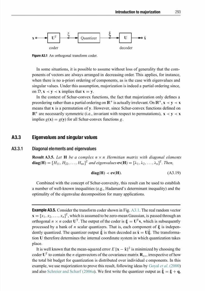
8/21/2019 Statistical Signal Processing of Complex-Valued Data.pdf
http://slidepdf.com/reader/full/statistical-signal-processing-of-complex-valued-datapdf 315/330
Introduction to majorization 293
decoder coder
Quantizer xξξξ
x UT U
Figure A3.1 An orthogonal transform coder.
In some situations, it is possible to assume without loss of generality that the com-
ponents of vectors are always arranged in decreasing order. This applies, for instance,
when there is no a-priori ordering of components, as is the case with eigenvalues and
singular values. Under this assumption, majorization is indeed a partial ordering since,
on D, x ≺ y ≺ x implies that x = y.
In the context of Schur-convex functions, the fact that majorization only defines a
preordering rather than a partial ordering on IR n is actually irrelevant. On IR n , x ≺ y ≺ xmeans that x is a permutation of y. However, since Schur-convex functions defined on
IR n are necessarily symmetric (i.e., invariant with respect to permutations), x ≺ y ≺ x
implies g (x) = g (y) for all Schur-convex functions g .
A3.3 Eigenvalues and singular values
A3.3.1 Diagonal elements and eigenvalues
Result A3.5. Let H be a complex n × n Hermitian matrix with diagonal elements
diag(H) = [ H 11, H 22, . . . , H nn ]T and eigenvalues ev(H) = [λ1, λ2, . . . , λn]T. Then,
diag(H) ≺ ev(H). (A3.19)
Combined with the concept of Schur-convexity, this result can be used to establish
a number of well-known inequalities (e.g., Hadamard’s determinant inequality) and the
optimality of the eigenvalue decomposition for many applications.
Example A3.5. Consider the transform coder shown in Fig. A3.1. The real random vector
x = [ x1, x2, . . . , xn]T, which is assumed to be zero-mean Gaussian, is passed through an
orthogonal n × n coder UT. The output of the coder is = UTx, which is subsequently
processed by a bank of n scalar quantizers. That is, each component of is indepen-
dently quantized. The quantizer output is then decoded as x = U. The transforma-
tion U therefore determines the internal coordinate system in which quantization takes
place.
It is well known that the mean-squared error E x − x2 is minimized by choosing the
coder UT to contain the n eigenvectors of the covariance matrix R x x , irrespective of howthe total bit budget for quantization is distributed over individual components. In this
example, we use majorization to prove this result, following ideas by Goyal et al . (2000)
and also Schreier and Scharf (2006a). We first write the quantizer output as = + q,
8/21/2019 Statistical Signal Processing of Complex-Valued Data.pdf
http://slidepdf.com/reader/full/statistical-signal-processing-of-complex-valued-datapdf 316/330
294 Appendix 3
where q = [q1, q2, . . . , qn]T denotes additive quantization noise. The variance of qi can
be modeled as
Eq2i
=d i f (bi ),
where d i ≥ 0 is the variance of component ξ i , and f (bi ) is a decreasing function of the
number of bits bi spent on quantizing ξ i . The function f characterizes the quantizer. We
may now express the MSE as
E x − x2 = E U( − )2 = E q2 =n
i=1
d i f (bi ).
We can assume without loss of generality that the components of are arranged such
that
d i ≥ d i+1, i = 1, . . . , n − 1.
Then, the minimum MSE solution requires that bi ≥ bi+1, i = 1, . . . , n − 1, because
f (bi ) is a decreasing function. With these assumptions, diag(R ξ ξ ) = [d 1, d 2, . . . , d n]T
and b = [b1, b2, . . . , bn]T are both ordered n-tuples.
For a fixed but arbitrary, ordered, bit assignment vector b, the MSE is a Schur-concave
function of the diagonal elements of R ξ ξ = UTR x x U. In order to show this, we note that
the MSE is of the form (A3.17) and f (bi ) ≤ f (bi+1), i = 1, . . . , n − 1, because f is
decreasing and bi ≥ bi+1.With this in mind, the majorization
diag(UTR x x U) ≺ ev(R x x )
establishes that theMSEis minimized if UTR x x U is diagonal. Therefore, U is determined
by the eigenvalue decomposition of R x x .
A3.3.2 Diagonal elements and singular values
For an arbitrary nonsquare, non-Hermitian matrix A ∈ Cm×n , the diagonal elements
and eigenvalues are generally complex, so that majorization would be possible only for
absolute values or real parts. Unfortunately, no such relationship exists. However, there
is the following comparison, which involves the singular values of A.
Result A3.6. With p = min(m, n) and |diag(A)| [| A11|, | A22|, . . . , | A pp |]T , we have
the weak majorization
|diag(A)
| ≺w sv(A). (A3.20)
This generalizes Result A3.5 to arbitrary matrices. Just as Result A3.5 establishes
many optimality results for the eigenvalue decomposition, Result A3.6 does so for the
singular value decomposition.
8/21/2019 Statistical Signal Processing of Complex-Valued Data.pdf
http://slidepdf.com/reader/full/statistical-signal-processing-of-complex-valued-datapdf 317/330
Introduction to majorization 295
A3.3.3 Partitioned matrices
In ResultA3.5, eigenvalues arecompared with diagonalelements.We shall now compare
the eigenvalues of the n
×n Hermitian matrix
H =H11 H12
HH12 H22
(A3.21)
with the eigenvalues of the corresponding block-diagonal matrix
H0 =
H11 0
0 H22
. (A3.22)
The submatrices are H11 ∈ Cn1×n1 , H12 ∈ Cn1×n2 , and H22 ∈ Cn2×n2 , where n = n1 +n2. Obviously, ev(H0) = (ev(H11), ev(H22)), and tr H = tr H0.
Result A3.7. There exists the majorization
ev(H0) ≺ = ev(H). (A3.23)
More generally, let
Hα =
H11 αH12
αHH12 H22
. (A3.24)
Then,
ev(Hα1)≺
ev(Hα2), 0
≤α1 < α2
≤1. (A3.25)
This shows that the “stronger” the off-diagonal blocks are, the more spread out the
eigenvalues become. An immediate consequence is the “block Hadamard inequality”
det H0 ≥ det H, or more generally, det Hα1 ≥ det Hα2
.
There is another result for block matrices of the form (A3.21) with n1 = n2 = n/2,
due to Thompson and Therianos (1972).
Result A3.8. Assuming that n1 = n2 and the eigenvalues of H , H11 , and H22 are each
ordered decreasingly, we have
k i=1
λi + λn−k +i ≤k
i=1
evi (H11) +k
i=1
evi (H22), k = 1, . . . , n1. (A3.26)
These inequalities are reminiscent of majorization. It is not necessarily majorization
because the partial sums on the left-hand side of (A3.26) need not be maximized for
some k . However, if
λi + λn−i+1 ≥ λi+1 + λn−i , i = 1, . . . , n1 − 1, (A3.27)
then (A3.26) becomes
[λ1 + λn , λ2 + λn−1, . . . , λn1 + λn−n1+1]T
≺ ev(H11) + ev(H22), (A3.28)
which is an actual majorization relation.
8/21/2019 Statistical Signal Processing of Complex-Valued Data.pdf
http://slidepdf.com/reader/full/statistical-signal-processing-of-complex-valued-datapdf 318/330
References
Adali, T. and Calhoun, V. D. (2007). Complex ICA of brain imaging data. IEEE Signal Processing
Mag., 24:136–139.
Adali, T., Li, H., Novey, M., and Cardoso, J.-F. (2008). Complex ICA using nonlinear functions.
IEEE Trans. Signal Processing , 56:4536–4544.
Amblard, P. O.,Gaeta,M.,andLacoume, J. L. (1996a).Statistics for complex variablesandsignals –
part I: variables. Signal Processing , 53:1–13.
(1996b). Statistics for complex variables and signals – part II: signals. Signal Processing ,
53:15–25.
Andersson, S. A. and Perlman, M. D. (1984). Two testing problems relating the real and complex
multivariate normal distribution. J. Multivariate Analysis, 15:21–51.
Anttila, L., Valkama, M., and Renfors, M. (2008). Circularity-based I/Q imbalance compensation
in wideband direct-conversion receivers. IEEE Trans. Vehicular Techn., 57:2099–2113.
Bangs, W. J. (1971). Array Processing with Generalized Beamformers. Ph.D. thesis, Yale Univer-
sity.
Bartmann, F. C. and Bloomfield, P. (1981). Inefficiency and correlation. Biometrika, 68:67–71.
Besson, O., Scharf, L. L., and Vincent, F. (2005). Matched direction detectors and estimators for
array processing with subspace steering vector uncertainties. IEEE Trans. Signal Processing ,
53:4453–4463.
Blahut, R. E. (1985). Fast Algorithms for Digital Signal Processing . Reading, MA: Addison-
Wesley.
Bloomfield, P. andWatson,G.S. (1975).Theinefficiency of least squares. Biometrika, 62:121–128.
Born, M. and Wolf, E. (1999). Principles of Optics. Cambridge: Cambridge University Press.
Boyles, R. A. and Gardner, W. A. (1983). Cycloergodic properties of discrete parameter non-
stationary stochastic processes. IEEE Trans. Inform. Theory, 29:105–114.
Brandwood, D. H. (1983). A complex gradient operator and its application in adaptive array theory.
IEE Proceedings H , 130:11–16.
Brown, W. M. and Crane, R. B. (1969). Conjugate linear filtering. IEEE Trans. Inform. Theory,
15:462–465.
Burt, W., Cummings, T., and Paulson, C. A. (1974). Mesoscale wind field over ocean. J. Geophys.
Res., 79:5625–5632.
Buzzi, S., Lops, M., and Sardellitti, S. (2006). Widely linear reception strategies for layered
space-time wireless communications. IEEE Trans. Signal Processing , 54:2252–2262.
Cacciapuoti, A. S., Gelli, G., and Verde, F. (2007). FIR zero-forcing multiuser detection and code
designs for downlink MC-CDMA. IEEE Trans. Signal Processing , 55:4737–4751.
Calman, J. (1978). On the interpretation of ocean current spectra. J. Physical Oceanography,
8:627–652.
8/21/2019 Statistical Signal Processing of Complex-Valued Data.pdf
http://slidepdf.com/reader/full/statistical-signal-processing-of-complex-valued-datapdf 319/330
References 297
Charge, P., Wang, Y., and Saillard, J. (2001). A non-circular sources direction finding method
using polynomial rooting. Signal Processing , 81:1765–1770.
Chen, M., Chen, Z., and Chen, G. (1997). Approximate Solutions of Operator Equations. Singa-
pore: World Scientific.
Chevalier, P. and Blin, A. (2007). Widely linear MVDR beamformers for the reception of an
unknown signal corrupted by noncircular interferences. IEEE Trans. Signal Processing ,
55:5323–5336.
Chevalier, P. and Picinbono, B. (1996). Complex linear-quadratic systems for detection and array
processing. IEEE Trans. Signal Processing , 44:2631–2634.
Chevalier, P. and Pipon, F. (2006). New insights into optimal widely linear array receivers for the
demodulation of BPSK, MSK, and GMSK interferences – application to SAIC. IEEE Trans.
Signal Processing , 54:870–883.
Cohen, L. (1966). Generalized phase-space distribution functions. J. Math. Phys., 7:781–
786.
Comon, P. (1994). Independent component analysis, a new concept? Signal Processing , 36:287–
314.
Conte, E., De Maio, A., and Ricci, G. (2001). GLRT-based adaptive detection algorithms for
range-spread targets. IEEE Trans. Signal Processing , 49:1336–1348.
Coxhead, P. (1974). Measuring the relationship between two sets of variables. Brit. J. Math. Statist.
Psych., 27:205–212.
Cramer, E. M. and Nicewander, W. A. (1979). Some symmetric, invariant measures of multivariate
association. Psychometrika, 44:43–54.
Davis, M. C. (1963). Factoring the spectral matrix. IEEE Trans. Automatic Control , 8:296–
305.
DeLathauwer, L. and DeMoor, B. (2002). On the blind separation of non-circular sources, in Proc.
EUSIPCO, pp. 99–102.
Delmas, J. P. (2004). Asymptotically minimum variance second-order estimation for noncir-
cular signals with application to DOA estimation. IEEE Trans. Signal Processing , 52:
1235–1241.
Delmas, J. P. and Abeida, H. (2004). Stochastic Cramer–Rao bound for noncircular signals with
application to DOA estimation. IEEE Trans. Signal Processing , 52:3192–3199.
Dietl, G., Zoltowski, M. D., and Joham, M. (2001). Recursive reduced-rank adaptive equalization
for wireless communication, Proc. SPIE , vol. 4395.
Drury, S. W. (2002). The canonical correlations of a 2×
2 block matrix with given eigenvalues.
Lin. Algebra Appl., 354:103–117.
Drury, S. W., Liu, S., Lu, C.-Y., Puntanen, S., and Styan, G. P. H. (2002). Some comments on
several matrix inequalities with applications to canonical correlations: historical background
and recent development. Sankhya A, 64:453–507.
Eaton, M. L. (1983). Multivariate Statistics: A Vector Space Approach. New York: Wiley.
Eriksson, J. and Koivunen, V. (2006). Complex random vectors and ICA models: identifiability,
uniqueness, and separability. IEEE Trans. Inform. Theory, 52:1017–1029.
Erkmen, B. I. (2008). Phase-Sensitive Light: Coherence Theory and Applications to Optical
Imaging . Ph.D. thesis, Massachusetts Institute of Technology.
Erkmen, B. I. andShapiro, J. H. (2006). Optical coherence theory forphase-sensitive light, in Proc.SPIE , volume 6305. Bellingham, WA: The International Society for Optical Engineering.
Fang, K.-T., Kotz, S., and Ng, K. W. (1990). Symmetric Multivariate and Related Distributions.
London: Chapman and Hall.
8/21/2019 Statistical Signal Processing of Complex-Valued Data.pdf
http://slidepdf.com/reader/full/statistical-signal-processing-of-complex-valued-datapdf 320/330
298 References
Ferguson, T. S. (1967). Mathematical Statistics: A Decision Theoretic Approach. New York:
Academic Press.
Ferrara, E. R. (1985). Frequency-domain implementations of periodically time-varying filters.
IEEE Trans. Acoustics, Speech, Signal Processing , 33:883–892.
Flandrin, P. (1999). Time–Frequency/Time–Scale Analysis. San Diego: Academic.
Gardner, W. A. (1986). Measurement of spectral correlation. IEEE Trans. Acoust. Speech Signal
Processing , 34:1111–1123.
(1988). Statistical Spectral Analysis. Englewood Cliffs, NJ: Prentice Hall.
(1993). Cyclic Wiener filtering: theory and method. IEEE Trans. Commun., 41:151–163.
Gardner, W. A., Brown, W. A., and Chen, C.-K. (1987). Spectral correlation of modulated signals,
part II: digital modulation. IEEE Trans. Commun., 35:595–601.
Gardner, W. A., Napolitano, A., and Paura, L. (2006). Cyclostationarity: half a century of research.
Signal Processing , 86:639–697.
Gelli, G., Paura, L., and Ragozini, A. R. P. (2000). Blind widely linear multiuser detection. IEEE
Commun. Lett., 4:187–189.
Gersho, A. and Gray, R. M. (1992). Vector Quantization and Signal Compression. Boston, MA:
Kluwer.
Gerstacker, H., Schober, R., and Lampe, A. (2003). Receivers with widely linear processing for
frequency-selective channels. IEEE Trans. Commun., 51:1512–1523.
Gladyshev, E. (1963). Periodically and almost periodically correlated random processes with
continuous time parameter. Theory Probab. Applic., 8:173–177.
Gladyshev, E. D. (1961). Periodically correlated random sequences. Soviet Math. Dokl., 2:385–
388.
Gleason, T. C. (1976). On redundancy in canonical analysis. Psych. Bull., 83:1004–1006.
Goh, S. L. and Mandic, D. P. (2007a). An augmented ACRTRL for complex valued recurrent
neural networks. Neural Networks, 20:1061–1066.
(2007b). An augmented extended Kalman filter algorithm for complex-valued recurrent neural
networks. Neural Computation, 19:1039–1055.
Goldstein, J. S., Reed, I. S., and Scharf, L. L. (1998). A multistage representation of the Wiener
filter based on orthogonal projections. IEEE Trans. Inform. Theory, 44:2943–2959.
Gonella, J. (1972). A rotary-component method for analysing meteorological and oceanographic
vector time series. Deep-Sea Res., 19:833–846.
Goodman, N. R. (1963). Statistical analysis based on a certain multivariate complex Gaussian
distribution (an introduction). Ann. Math. Statist., 34:152–177.
Gorman, J. D. and Hero, A. (1990). Lower bounds for parametric estimation with constraints.
IEEE Trans. Inform. Theory, 26:1285–1301.
Goyal, V. K., Zhuang, J., and Vetterli, M. (2000). Transform coding with backward adaptive
updates. IEEE Trans. Inform. Theory, 46:1623–1633.
Grettenberg, T. L. (1965). A representation theorem for complex normal processes. IEEE Trans.
Inform. Theory, 11:305–306.
Haardt, M. and Roemer, F. (2004). Enhancements of unitary ESPRIT for non-circular sources, in
Proc. ICASSP , pp. 101–104.
Hanson, B., Klink,K.,Matsuura,K.,Robeson,S.M.,andWillmott, C. J. (1992).Vectorcorrelation:
review, exposition, and geographic application. Ann. Association Am. Geographers, 82:103– 116.
Hanssen, A. and Scharf, L. (2003). A theory of polyspectra for nonstationary stochastic processes.
IEEE Trans. Signal Processing , 51:1243–1252.
8/21/2019 Statistical Signal Processing of Complex-Valued Data.pdf
http://slidepdf.com/reader/full/statistical-signal-processing-of-complex-valued-datapdf 321/330
References 299
Hindberg, H., Birkelund, Y., Øigard, T. A., and Hanssen, A. (2006). Kernel-based estimators
for the Kirkwood–Rihaczek time-frequency spectrum, in Proc. European Signal Processing
Conference.
Horn, R. A. and Johnson, C. R. (1985). Matrix Analysis. Cambridge: Cambridge University Press.
Hotelling, H. (1936). Relations between two sets of variates. Biometrika, 28:321–377.
Hua, Y., Nikpour, M., and Stoica, P. (2001). Optimal reduced-rank estimation and filtering. IEEE
Trans. Signal Processing , 49:457–469.
Izzo, L. and Napolitano, A. (1997). Higher-order statistics for Rice’s representation of cyclosta-
tionary signals. Signal Processing , 56:179–292.
(1998). Multirate processing of time-series exhibiting higher-order cyclostationarity. IEEE
Trans. Signal Processing , 46:429–439.
Jeon, J. J., Andrews, J. G., and Sung, K. M. (2006). The blind widely linear minimum out-
put energy algorithm for DS-CDMA systems. IEEE Trans. Signal Processing , 54:1926–
1931.
Jezek, J. and Kucera, V. (1985). Efficient algorithm for matrix spectral factorization. Automatica,
21:663–669.
Jones, A. G. (1979). On the difference between polarisation and coherence. J. Geophys., 45:223–
229.
Jones, R. C. (1941). New calculus for the treatment of optical systems. J. Opt. Soc. Am., 31:488–
493.
Jouny, I. I. andMoses,R. L. (1992). The bispectrum of complex signals: definitions andproperties.
IEEE Trans. Signal Processing , 40:2833–2836.
Jupp, P. E. and Mardia, K. V. (1980). A general correlation coefficient for directional data and
related regression problems. Biometrika, 67:163–173.
Kelly, E. J. (1986). An adaptive detection algorithm. IEEE Trans. Aerosp. Electron. Syst., 22:115–
127.
Kelly, E. J. and Root, W. L. (1960). A representation of vector-valued random processes. Group
Rept. MIT Lincoln Laboratory, no. 55–21.
Kraut, S., Scharf, L. L., and McWhorter, L. T. (2001). Adaptive subspace detectors. IEEE Trans.
Signal Processing , 49:1–16.
Lampe, A., Schober, R., and Gerstacker, W. (2002). A novel iterative multiuser detector for
complex modulation schemes. IEEE J. Sel. Areas Commun., 20:339–350.
Lee, E. A. and Messerschmitt, D. G. (1994). Digital Communication. Boston, MA: Kluwer.
Lehmann, E. L. and Romano, J. P. (2005). Testing Statistical Hypotheses, 2nd edn. New York:
Springer.
Li, H. and Adali, T. (2008). A class of complex ICA algorithms based on the kurtosis cost function.
IEEE Trans. Neural Networks, 19:408–420.
Lilly, J. M. and Gascard, J.-C. (2006). Wavelet ridge diagnosis of time-varying elliptical signals
with application to an oceanic eddy. Nonlin. Processes Geophys., 13:467–483.
Lilly, J. M. and Park, J. (1995). Multiwavelet spectral and polarization analysis. Geophys. J. Int.,
122:1001–1021.
Loeve, M. (1978). Probability Theory II , 4th edn. New York: Springer.
Mandic, D. P. and Goh, V. S. L. (2009). Complex Valued Nonlinear Adaptive Filters. New York:
Wiley.Mardia, K. V., Kent, J. T., and Bibby, J. M. (1979). Multivariate Analysis. New York: Academic.
Marshall, A. W. and Olkin, I. (1979). Inequalities: Theory of Majorization and Its Applications.
New York: Academic.
8/21/2019 Statistical Signal Processing of Complex-Valued Data.pdf
http://slidepdf.com/reader/full/statistical-signal-processing-of-complex-valued-datapdf 322/330
300 References
Martin, W. (1982). Time–frequency analysis of random signals, in Proc. Int. Conf. Acoustics.,
Speech, Signal Processing , pp. 1325–1328.
Martin, W. and Flandrin, P. (1985). Wigner–Ville spectral analysis of nonstationary processes.
IEEE Trans. Acoustics, Speech, Signal Processing , 33:1461–1470.
Marzetta, T. L. (1993). A simple derivation of the constrained multiple parameter Cramer–Rao
bound. IEEE Trans. Signal Processing , 41:2247–2249.
McWhorter, L. T. and Scharf, L. (1993a). Geometry of the Cramer–Rao bound. Signal Processing ,
31:301–311.
(1993b). Cramer–Rao bounds for deterministic modal analysis. IEEE Trans. Signal Processing ,
41:1847–1865.
(1993c). Properties of quadratic covariance bounds, in Proc. 27th Asilomar Conf. Signals,
Systems, Computers, pp. 1176–1180.
McWhorter, T. and Schreier, P. (2003). Widely-linear beamforming, in Proc. 37th Asilomar Conf.
Signals, Systems, Comput., pp. 753–759.
Mirbagheri, A., Plataniotis, N., and Pasupathy, S. (2006). An enhanced widely linear CDMA
receiver with OQPSK modulation. IEEE Trans. Commun., 54:261–272.
Mitra, S. K. (2006). Digital Signal Processing , 3rd edn. Boston, MA: McGraw-Hill.
Molle, J. W. D. and Hinich, M. J. (1995). Trispectral analysis of stationary random time series.
IEEE Trans. Signal Processing , 97:2963–2978.
Mooers, C. N. K. (1973). A technique for the cross spectrum analysis of pairs of complex-valued
time series, components and rotational invariants. Deep-Sea Res., 20:1129–1141.
Morgan, D. R. (2006). Variance and correlation of square-law detected allpass channels with
bandpass harmonic signals in Gaussian noise. IEEE Trans. Signal Processing , 54:2964–
2975.
Morgan, D. R. and Madsen, C. K. (2006). Wide-band system identification using multiple tones
with allpass filters and square-law detectors. IEEE Trans. Circuits Systems I , 53:1151–1165.
Mueller, H. (1948). The foundation of optics. J. Opt. Soc. Am., 38:661–672.
Mullis, C. T. and Scharf, L. L. (1996). Applied Probability. Course notes for ECE5612, Univ. of
Colorado, Boulder, CO.
Napolitano,A. and Spooner, C. M. (2001). Cyclic spectral analysisof continuous-phase modulated
signals. IEEE Trans. Signal Processing , 49:30–44.
Napolitano, A. and Tanda, M. (2004). Doppler-channel blind identification for noncircular trans-
missions in multiple-access systems. IEEE Trans. Commun., 52:2073–2078.
Navarro-Moreno, J., Ruiz-Molina, J. C., and Fernandez-Alcala, R. M. (2006). Approximate series
representations of linear operations on second-order stochastic processes: application to
simulation. IEEE Trans. Inform. Theory, 52:1789–1794.
Neeser, F. D. and Massey, J. L. (1993). Proper complex random processes with applications to
information theory. IEEE Trans. Inform. Theory, 39:1293–1302.
Nilsson, R., Sjoberg, F., and LeBlanc, J. P. (2003). A rank-reduced LMMSE canceller for narrow-
band interference suppression in OFDM-based systems. IEEE Trans. Commun., 51:2126–
2140.
Novey, M. and Adali, T. (2008a). Complex ICA by negentropy maximization. IEEE Trans. Neural
Networks, 19:596–609.
(2008b). On extending the complex FastICA algorithm to noncircular sources. IEEE Trans.Signal Processing , 56:2148–2154.
Olhede, S. and Walden, A. T. (2003a). Polarization phase relationships via multiple Morse
wavelets. I. Fundamentals. Proc. Roy. Soc. Lond. A Mat., 459:413–444.
8/21/2019 Statistical Signal Processing of Complex-Valued Data.pdf
http://slidepdf.com/reader/full/statistical-signal-processing-of-complex-valued-datapdf 323/330
References 301
(2003b). Polarization phase relationships via multiple Morse wavelets. II. Data analysis. Proc.
Roy. Soc. Lond. A Mat., 459:641–657.
Ollila, E. (2008). On the circularity of a complex random variable. IEEE Signal Processing Lett.,
15:841–844.
Ollila, E. and Koivunen, V. (2004). Generalized complex elliptical distributions, in Proc. SAM
Workshop, pp. 460–464.
(2009). Complex ICA using generalized uncorrelating transform. Signal Processing , 89:365–
377.
Pflug, L. A., Ioup, G. E., Ioup, J. W., and Field, R. L. (1992). Properties of higher-order correlations
and spectra for bandlimited, deterministic transients. J. Acoust. Soc. Am., 91:975–988.
Picinbono, B. (1994). On circularity. IEEE Trans. Signal Processing , 42:3473–3482.
(1996). Second-order complex random vectors and normal distributions. IEEE Trans. Signal
Processing , 44:2637–2640.
Picinbono, B. and Bondon, P. (1997). Second-order statistics of complex signals. IEEE Trans.
Signal Processing , 45:411–419.
Picinbono, B. and Chevalier, P. (1995). Widely linear estimation with complex data. IEEE Trans.
Signal Processing , 43:2030–2033.
Picinbono, B.andDuvaut,P. (1988).Optimal linear-quadraticsystems fordetectionandestimation.
IEEE Trans. Inform. Theory, 34:304–311.
Poor, H. V. (1998). An Introduction to Signal Detection and Estimation. New York: Springer.
Proakis, J. G. (2001). Digital Communications, 4th edn. Boston, MA: McGraw-Hill.
Ramsay, J. O., ten Berge, J., and Styan, G. P. H. (1984). Matrix correlation. Psychometrika,
49:402–423.
Reed, I. S., Mallett, J. D., and Brennan, L. E. (1974). Rapid convergence rate in adaptive arrays.
IEEE Trans. Aerosp. Electron. Syst., 10:853–863.
Renyi, A. (1959). On measures of dependence. Acta Math. Acad. Sci. Hungary, 10:441–451.
Richmond, C. D. (2006). Mean-squared error and threshold SNR prediction of maximum like-
lihood signal parameter estimation with estimated colored noise covariances. IEEE Trans.
Inform. Theory, 52:2146–2164.
Rihaczek, A. W. (1968). Signal energy distribution in time and frequency. IEEE Trans. Inform.
Theory, 14:369–374.
Rivet, B., Girin, L., and Jutten, C. (2007). Log-Rayleigh distribution: a simple and efficient
statistical representation of log-spectral coefficients. IEEE Trans. Audio, Speech, Language
Processing , 15:796–802.
Robert, P. and Escoufier, Y. (1976). A unifying tool for linear multivariate statistical methods: the
RV-coefficient. Appl. Statist., 25:257–265.
Robey, F. C., Fuhrmann, D. R., Kelly, E. J., and Nitzberg, R. A. (1992). A CFAR adaptive matched
filter detector. IEEE Trans. Aerosp. Electron. Syst., 28:208–216.
R omer, F. and Haardt, M. (2007). Deterministic Cramer–Rao bounds for strict sense non-circular
sources, in Proc. ITG/IEEE Workshop on Smart Antennas.
(2009). Multidimensional unitary tensor-esprit for non-circular sources, in Proc. ICASSP .
Roueff, A., Chanussot, J., and Mars, J. I. (2006). Estimation of polarization parameters using
time-frequency representations and its application to waves separation. Signal Processing ,
86:3714–3731.Rozanov, Y. A. (1963). Stationary Random Processes. San Francisco, CA: Holden-Day.
Rozeboom, W. W. (1965). Linear correlation between sets of variables. Psychometrika, 30:
57–71.
8/21/2019 Statistical Signal Processing of Complex-Valued Data.pdf
http://slidepdf.com/reader/full/statistical-signal-processing-of-complex-valued-datapdf 324/330
302 References
Rubin-Delanchy, P. and Walden, A. T. (2007). Simulation of improper complex-valued sequences.
IEEE Trans. Signal Processing , 55:5517–5521.
(2008). Kinematics of complex-valued time series. IEEE Trans. Signal Processing , 56:4189–
4198.
Rykaczewski, P., Valkama, M., and Renfors, M. (2008). On the connection of I/Q imbalance
and channel equalization in direct-conversion transceivers. IEEE Trans. Vehicular Techn.,
57:1630–1636.
Sampson, P. D., Streissguth, A. P., Barr, H. M., and Bookstein, F. L. (1989). Neurobehavioral
effects of prenatal alcohol: part II. Partial least squares analysis. Neurotoxicology Teratology,
11:477–491.
Samson, J. C. (1980). Comments on polarization and coherence. J. Geophys., 48:195–198.
Scharf, L. L. (1991). Statistical Signal Processing . Reading, MA: Addison-Wesley.
Scharf, L. L., Chong, E. K. P., Zoltowski, M. D., Goldstein, J. S., and Reed, I. S. (2008). Subspace
expansion and the equivalence of conjugate direction and multistage Wiener filters. IEEE
Trans. Signal Processing , 56:5013–5019.
Scharf, L. L. and Friedlander, B. (1994). Matched subspace detectors. IEEE Trans. Signal Pro-
cessing , 42:2146–2157.
(2001).Toeplitz and Hankel kernels forestimatingtime-varyingspectra of discrete-time random
processes. IEEE Trans. Signal Processing , 49:179–189.
Scharf, L. L., Schreier, P. J., and Hanssen, A. (2005). The Hilbert space geometry of the Rihaczek
distribution for stochastic analytic signals. IEEE Signal Processing Lett., 12:297–300.
Schreier, P. J. (2008a). Bounds on the degree of impropriety of complex random vectors. IEEE
Signal Processing Lett., 15:190–193.
(2008b). Polarization ellipse analysis of nonstationary random signals. IEEE Trans. Signal
Processing , 56:4330–4339.
(2008c). A unifying discussion of correlation analysis forcomplex randomvectors. IEEE Trans.
Signal Processing , 56:1327–1336.
Schreier, P. J., Adalı, T., and Scharf, L. L. (2009). On ICA of improper and noncircular sources,
in Proc. Int. Conf. Acoustics, Speech, Signal Processing .
Schreier, P. J. and Scharf, L. L. (2003a). Second-order analysis of improper complex random
vectors and processes. IEEE Trans. Signal Processing , 51:714–725.
(2003b). Stochastic time-frequency analysis using the analytic signal: why the complementary
distribution matters. IEEE Trans. Signal Processing , 51:3071–3079.
(2006a). Canonical coordinates for transform coding of noisy sources. IEEE Trans. Signal
Processing , 54:235–243.
(2006b). Higher-order spectral analysis of complex signals. Signal Processing , 86:3321–
3333.
Schreier, P. J., Scharf, L. L., and Hanssen, A. (2006). A generalized likelihood ratio test for
impropriety of complex signals. IEEE Signal Processing Lett., 13:433–436.
Schreier, P. J., Scharf, L. L., and Mullis, C. T. (2005). Detection and estimation of improper
complex random signals. IEEE Trans. Inform. Theory, 51:306–312.
Schur, I. (1923). Uber eine Klasse von Mittelbildungen mit Anwendungen auf die Determinan-
tentheorie. Sitzungsber. Berliner Math. Ges., 22:9–20.
Serpedin, E., Panduru, F., Sari, I., and Giannakis, G. B. (2005). Bibliography on cyclostationarity.Signal Processing , 85:2233–2303.
Shapiro, J. H. and Erkmen, B. I. (2007). Imaging with phase-sensitive light, in Int. Conf. on
Quantum Information. New York: Optical Society of America.
8/21/2019 Statistical Signal Processing of Complex-Valued Data.pdf
http://slidepdf.com/reader/full/statistical-signal-processing-of-complex-valued-datapdf 325/330
References 303
Slepian, D. (1954). Estimation of signal parameters in the presence of noise. Trans. IRE Prof.
Group Inform. Theory, 3:68–89.
Spurbeck, M. S. and Mullis, C. T. (1998). Least squares approximation of perfect reconstruction
filter banks. IEEE Trans. Signal Processing , 46:968–978.
Spurbeck, M. S. and Schreier, P. J. (2007). Causal Wiener filter banks for periodically correlated
time series. Signal Processing , 87:1179–1187.
Srivastava, M. S. (1965). On the complex Wishart distribution. Ann. Math. Statist., 36:313–
315.
Stewart, D. and Love, W. (1968). A general canonical correlation index. Psych. Bull., 70:160–
163.
Stoica, P. and Ng, B. C. (1998). On the Cramer–Rao bound under parametric constraints. IEEE
Signal Processing Lett., 5:177–179.
Stokes, G. G. (1852). On the composition and resolution of streams of polarized light from
different sources. Trans. Cambr. Phil. Soc., 9:399–423.
Taubock, G. (2007). Complex noise analysis of DMT. IEEE Trans. Signal Processing , 55:5739–
5754.
Thompson, R. C. and Therianos, S. (1972). Inequalities connecting the eigenvalues of a Hermitian
matrix with the eigenvalues of complementary principal submatrices. Bull. Austral. Math.
Soc., 6:117–132.
Tishler, A. and Lipovetsky, S. (2000). Modelling and forecasting with robust canonical analysis:
method and application. Comput. Op. Res., 27:217–232.
van den Bos, A. (1994a). Complex gradient and Hessian. IEE Proc. Vision, Image, Signal Pro-
cessing , 141:380–383.
(1994b). A Cramer–Rao lower bound for complex parameters. IEEE Trans. Signal Processing ,
42:2859.
(1995). The multivariate complex normal distribution – a generalization. IEEE Trans. Inform.
Theory, 41:537–539.
Van Trees, H. L. (2001). Detection, Estimation, and Modulation Theory: Part I . New York: Wiley.
Van Trees, H. L. and Bell, K. L., editors (2007). Bayesian Bounds for Parameter Estimation and
Nonlinear Filtering/Tracking . New York: IEEE and Wiley-Interscience.
Wahlberg, P. and Schreier, P. J. (2008). Spectral relations for multidimensional complex improper
stationary and (almost) cyclostationary processes. IEEE Trans. Inform. Theory, 54:1670–
1682.
Walden, A. T. and Rubin-Delanchy, P. (2009). On testing for impropriety of complex-valued
Gaussian vectors. IEEE Trans. Signal Processing , 57:825–834.
Weinstein, E. and Weiss, A. J. (1988). A general class of lower bounds in parameter estimation.
IEEE Trans. Inform. Theory, 34:338–342.
Weippert, M. E., Hiemstra, J. D., Goldstein, J. S., and Zoltowski, M. D. (2002). Insights from the
relationship between the multistage Wiener filter and the method of conjugated gradients,
Proc. IEEE Workshop on Sensor Array Multichannel Signal Processing , pp. 388–392.
Weiss, A. J. and Weinstein, E. (1985). A lower bound on the mean squared error in random
parameter estimation. IEEE Trans. Inform. Theory, 31:680–682.
Wiener, N. and Masani, P. (1957). The prediction theory of multivariate stochastic processes,
part I. Acta Math., 98:111–150.(1958). The prediction theory of multivariate stochastic processes, part II. Acta Math., 98:93–
137.
8/21/2019 Statistical Signal Processing of Complex-Valued Data.pdf
http://slidepdf.com/reader/full/statistical-signal-processing-of-complex-valued-datapdf 326/330
304 References
Wilson, G. T. (1972). The factorization of matricial spectral densities. SIAM J. Appl. Math.,
23:420–426.
Wirtinger, W. (1927). Zur formalen Theorie der Funktionen von mehr komplexen Ver anderlichen.
Math. Ann., 97:357–375.
Witzke, M. (2005). Linear and widely linear filtering applied to iterative detection of generalized
MIMO signals. Ann. Telecommun., 60:147–168.
Wold, H. (1975). Path models with latent variables: the NIPALS approach, in Blalock, H. M.,
editor, Quantitative Sociology: International Perspectives on Mathematical and Statistical
Modeling . New York: Academic, pp. 307–357.
(1985). Partial least squares, in Kotz, S. and Johnson, N. L., editors, Encyclopedia of the
Statistical Sciences, New York: Wiley, pp. 581–591.
Wolf, E. (1959). Coherence properties of partially polarized electromagnetic radiation. Nuovo
Cimento, 13:1165–1181.
Wooding, R. A. (1956). The multivariate distribution of complex normal variables. Biometrika,
43:212–215.
Yanai,H. (1974).Unification of varioustechniques of multivariate analysisbymeansofgeneralized
coefficient of determination (G.C.D.). J. Behaviormetrics, 1:45–54.
Yoon, Y. C. and Leib, H. (1997). Maximizing SNR in improper complex noise and applications
to CDMA. IEEE Commun. Letters, 1:5–8.
Youla, D. C. (1961). On the factorization of rational matrices. IRE Trans. Inform. Theory, 7:172–
189.
Zou, Y., Valkama, M., and Renfors, M. (2008). Digital compensation of I/Q imbalance effects
in space-time coded transmit diversity systems. IEEE Trans. Signal Processing , 56:2496–
2508.

8/21/2019 Statistical Signal Processing of Complex-Valued Data.pdf
http://slidepdf.com/reader/full/statistical-signal-processing-of-complex-valued-datapdf 327/330
Index
aliasing, 236
almost cyclostationary process, 251
almost periodic function, 251
ambiguity function, 232analytic function, 280
analytic signal, 11
higher-order spectra, 218 – 221
nonstationary, 235, 245
N th-order circular, 221
WSS, 201
applications (survey), 27
augmented
covariance function, 55
covariance matrix, 34, 36
eigenvalue decomposition, 62
expansion-coefficient matrix, 161frequency-response matrix, 201
information matrix, 161
matrix, 32
mean vector, 34
PSD matrix, 55
sensitivity matrix, 161
vector, 31
baseband signal, 9, 201
Bayes detector, 180
Bayes risk, 180
Bayesian point of view, 116, 152 – 157 beamformer, 143
Bedrosian’s theorem, 14
best linear unbiased estimator, see LMVDR
estimation
bicorrelation, 217
bispectrum, 217
blind source separation, 81 – 84
BLUE, see LMVDR estimation
BPSK spectrum, 257
C-ESD, 233
C-PSD, 55, 197connection with C-ESD, 233
nonstationary process, 234
canonical correlations, 93 – 100
between x and x∗, 65
for rank reduction, 135 – 137
invariance properties, 97 – 100
Cauchy distribution, 46Cauchy–Riemann equations, 280, 281
CCA, see canonical correlations
CFAR matched subspace detector, 193
chain rule (for differentiating non-holomorphic
functions), 281
characteristic function, 49 – 50
Cholesky decomposition, 272
circular, 53
N th-order, 54, 221
circularity coefficients, 65 – 69
circularity spectrum, 65 – 69
circularly polarized, 7, 206, 246Cohen’s class, 240
coherence
between rotary components (WSS), 211 – 216
cyclic spectral (cyclostationary), 254
time–frequency (nonstationary), 238, 244, 247
complementary
covariance function, 55
covariance matrix, 34
characterization, 36, 69
energy spectral density, see C-ESD
expansion-coefficient matrix, 161
Fisher information, 167information matrix, 161
power spectral density, see C-PSD
Rihaczek distribution, see Rihaczek distribution
sensitivity matrix, 161
spectral correlation, see spectral correlation
variance, 22
complex . . ., see corresponding entry without
“complex”
concentration ellipsoid, 127
conditional mean estimator, 119 – 121
conformal function, 280
conjugate covariance, see complementarycovariance
conjugate differential operator, 279
contour (pdf), 42, 46
8/21/2019 Statistical Signal Processing of Complex-Valued Data.pdf
http://slidepdf.com/reader/full/statistical-signal-processing-of-complex-valued-datapdf 328/330
306 Index
correlation analysis, 85 – 110
correlation coefficient, 22, 42, 86 – 93, 102 – 108
based on canonical correlations, 103 – 106
based on half-canonical correlations, 106 – 107
based on PLS correlations, 108for real data, 86
reflectional, 87 – 91, 94 – 97
rotational, 87 – 91, 94 – 97
total, 87 – 91, 94 – 97
correlation function, see covariance function
correlation spread, 108
covariance function, 54
CR-TFD, see Rihaczek distribution
Cramer–Loeve spectral representation, see spectral
representation
Cramer–Rao bound, 163 – 170
stochastic, 171 – 174CS process, see cyclostationary process
cumulant, 52
cycle frequency, 252
cyclic
complementary correlation function, 252
complementary power spectral density, 252 – 260
correlation function, 252
periodogram, 255
power spectral density, 252 – 260
spectral coherence, 254
Wiener filter, 260 – 268
cycloergodic, 268cyclostationary process, 250 – 268
connection with vector WSS process, 262
estimation of, 260 – 268
spectral representation, 251 – 253
damped harmonic oscillator, 5
decreasing function, 289
deflection, 184
degree of impropriety, 70 – 77
degree of polarization, 109, 211 – 215,
245
demodulation, 13detection, 177 – 194
nonstationary process, 230
probability, 178
DFT, 17
differential calculus, 277 – 286
differential entropy, see entropy
discrete Fourier transform, 17
dual-frequency spectrum, see spectral correlation
efficient estimator, 159, 171
eigenfunction, 224
eigenvalue decomposition, 62, 270electromagnetic polarization, 6
elliptical distribution, 44 – 47
energy signal, 234
energy spectral density, see ESD
entropy, 37, 67
envelope, 9
error score, 153
ESD, 233 – 234estimation, 116 – 149
cyclostationary process, 260 – 268
linear MMSE, 121 – 129
linear MVDR, 137 – 144
MMSE, 119 – 121
nonstationary process, 227 – 229
performance bounds, 151 – 175
reduced-rank, 132 – 137
widely linear MMSE, 129 – 132
widely linear MVDR, 143
widely linear–quadratic, 144 – 149
WSS process, see Wiener filter EVD, see eigenvalue decomposition
expansion-coefficient matrix, 158
augmented, 161
complementary, 161
expectation operator, 38, 153
extreme point, 70
false-alarm probability, 178
fast Fourier transform, 17
FFT, 17
Fischer determinant inequality, 274
Fisher information matrix, 162 – 170complementary, 167
Fisher score, 162 – 170
Fisher–Bayes bound, 171 – 174
Fisher–Bayes score, 171 – 174
four-corners diagram, 231
frequency-shift filter, 260 – 268
frequentist point of view, 116, 152 – 157
FRESH filter, 260 – 268
Gaussian distribution, 19 – 23, 39 – 44
characteristic function, 50
generalized complex differential operator, 278generalized likelihood-ratio test, see GLRT
generalized sidelobe canceler, 139 – 142
generating matrix (elliptical pdf), 45
global frequency variable, 231 – 232
global time variable, 231 – 232
GLRT for
correlation structure, 110 – 114
impropriety, 77 – 81
independence, 112
sphericity, 112
goniometer, 142
gradient, 280 – 282Grammian matrix, 119, 272
Grettenberg’s theorem, 53
GSC, 139 – 142

8/21/2019 Statistical Signal Processing of Complex-Valued Data.pdf
http://slidepdf.com/reader/full/statistical-signal-processing-of-complex-valued-datapdf 329/330
Index 307
Hadamard’s determinant inequality, 274, 287
half-canonical correlations, 93 – 97, 100
for rank reduction, 133 – 135
invariance properties, 100
harmonic oscillator, 5harmonizable, 230
Hermitian matrix, 270
Hessian matrix, 283 – 286
higher-order moments, 50 – 54, 217 – 222, 247
higher-order spectra, 217 – 222, 248
analytic signal, 219 – 222
Hilbert space of random variables, 117 – 119
Hilbert transform, 11 – 15
holomorphic function, 279 – 280
HR-TFD, see Rihaczek distribution
hypothesis test, see test
I/Q imbalance, 71
ICA, 81 – 84
improper, 35
maximally, 22, 44, 76
impropriety
degree of, 70 – 77
test for, 77 – 81
in-phase component, 9
increasing function, 289
independent component analysis, 81 – 84
information matrix, 158
augmented, 161complementary, 161
Fisher, 162 – 170
inner product, 33, 117 – 119
instantaneous
amplitude, 14
frequency, 14
phase, 14
invariant statistic, 181
invariant test, 189
inverse matrix, 274 – 276
Jacobian, 280 jointly proper, 41
Jones calculus, 7, 214
Jones vector, 7, 213 – 215
Karhunen–Loeve expansion, 224
Karlin–Rubin theorem, 188
Kramers–Kronig relation, 12
Lanczos kernel, 167
left–circularly polarized, 7, 208
level curve (pdf), 42, 46
likelihood-ratio test, 179linear minimum mean-squared error, see LMMSE
linear minimum variance distortionless response
estimation, see LMVDR estimation
linear–conjugate-linear, see widely linear
linearly polarized, 6, 208
Lissajous figure, 6
LMMSE estimation, 121 – 129
gain, 127Gaussian, 128
LMVDR estimation, 137 – 144, 156
widely linear, 143
Loeve spectrum, see spectral correlation
local frequency variable, 231 – 232
local time variable, 231 – 232
log-likelihood ratio, 179
majorization, 287 – 295
weak, 288
matched filter, 138, 144, 183
noncoherent adaptive, 143matched subspace detector, 190 – 194
CFAR, 193
matrix
factorizations, 270 – 272
Grammian, 272
Hermitian, 270
inverse, 274 – 276
normal, 270
partial ordering, 273
positive definite, 272
positive semidefinite, 272
pseudo-inverse, 275square root, 272
maximal invariant, 98
maximally improper, 22, 44, 76
maximum likelihood, see ML
measurement score, 154
Mercer’s expansion, 224
minimal statistic, 181
minimum mean-squared error, see MMSE
Minkowski determinant inequality, 274
mixing matrix, 81
ML estimation, 156
of covariance matrices, 48MLR, see half-canonical correlations
MMSE estimation, 119 – 121
modulation, 8 – 10
monomial matrix, 81
Moore–Penrose inverse, 275
Mueller calculus, 214
multivariate association, 85 – 108
multivariate linear regression, see half-canonical
correlations
MVDR estimation, see LMVDR estimation
Neyman–Pearson lemma (detector), 179noncircular, 53
strict-sense, see maximally improper
noncoherent matched subspace detector, 190 – 194

8/21/2019 Statistical Signal Processing of Complex-Valued Data.pdf
http://slidepdf.com/reader/full/statistical-signal-processing-of-complex-valued-datapdf 330/330
308 Index
nonstationary process, 223 – 248
analytic, 235, 245
detection of, 230
discrete time, 236
estimation of, 227 – 229spectral representation, 230 – 237
normal, see Gaussian
normal matrix, 270
N th-order circular, 54, 221
N th-order proper, see N th-order circular
orthogonal increments, 199
orthogonality principle, 120
PAM spectrum, 255 – 258
partial least squares, 93 – 97, 101
partial orderingmajorization, 289
matrices, 273
PCA, see principal components
pdf, see probability density function
pdf generator (elliptical), 44
performance bounds, 151 – 175
Bayesian, 170 – 174
deterministic, 157 – 170
frequentist, 157 – 170
stochastic, 170 – 174
performance comparison
between WL and linear detection, 186 – 188,230
between WL and LMMSE estimation, 131,
229
periodically correlated, see cyclostationary
periodogram (cyclic), 255
phase splitter, 11
phasor, 5
PLS, 93 – 97, 101
polarization, 6 – 8, 211 – 215, 245
circular, 7, 206, 246
degree of, 109, 211 – 215, 245
ellipse, 6, 23, 206 – 211, 242 – 247left circular, 7, 208
linear, 6, 208
right circular, 7, 208
positive definite matrix, 272
positive semidefinite matrix, 272
power
detection, 179
distribution (time–frequency), 237
random process, 56
random vector, 37
power signal, 234
power spectral density, see PSD preordering (majorization), 289
principal components, 63
principal domain, 218
probability density function, 38 – 47
Cauchy, 46
elliptical, 44 – 47
Gaussian, 19 – 23, 39 – 44
Rayleigh, 44t , 46
Wishart, 47
probability distribution function, 38
projection, 276
proper, 35
complex baseband signal, 56
jointly, 41
N th-order, see N th-order circular
random process, 56
PSD, 55, 197
connection with ESD, 233
digital modulation schemes, 255 – 258nonstationary process, 234
pseudo-covariance, see complementary covariance
pseudo-inverse, 275
PSK spectrum, 255 – 258
QAM spectrum, 255 – 258
QPSK spectrum, 257
quadratic form, 34, 145, 284
quadrature component, 9
quadrature modulation, 9
rank reduction, 64, 132 – 137Rayleigh distribution, 44
Rayleigh resolution limit, 167
receiver operating characteristic, 181
rectilinear, see maximally improper
reduced-rank estimation, 132 – 137
redundancy index, 106
reflectional correlation coefficient, 87 – 91, 94 – 97
reflectional cyclic spectral coherence, 254
relation matrix, see complementary covariance
right-circularly polarized, 7, 208
Rihaczek distribution, 232, 237 – 242
estimation of, 240 – 242ROC curve, 181
rotary components
nonstationary, 243
WSS, 205 – 211
rotating phasor, 5
rotational correlation coefficient, 87 – 91, 94 – 97
rotational cyclic spectral coherence, 254
Schur complement, 270
Schur-concave, 289
Schur-convex, 289
score function, 154Fisher, 162 – 170
Fisher–Bayes, 171 – 174
second-order stationary, 55