statistical signal processing for graphs by nadya … · statistical signal processing for graphs...
TRANSCRIPT

Statistical Signal Processing for Graphs
by
Nadya Travinin Bliss
A Dissertation Presented in Partial Fulfillmentof the Requirements for the Degree
Doctor of Philosophy
Approved April 2015 by theGraduate Supervisory Committee:
Manfred Laubichler, Co-ChairCarlos Castillo-Chavez, Co-ChairAntonia Papandreou-Suppappola
ARIZONA STATE UNIVERSITY
May 2015

ABSTRACT
Analysis of social networks has the potential to provide insights into wide range of
applications. As datasets continue to grow, a key challenge is the lack of a widely
applicable algorithmic framework for detection of statistically anomalous networks
and network properties. Unlike traditional signal processing, where models of truth
or empirical verification and background data exist and are often well defined, these
features are commonly lacking in social and other networks. Here, a novel algorithmic
framework for statistical signal processing for graphs is presented. The framework is
based on the analysis of spectral properties of the residuals matrix. The framework
is applied to the detection of innovation patterns in publication networks, leveraging
well-studied empirical knowledge from the history of science. Both the framework
itself and the application constitute novel contributions, while advancing algorithmic
and mathematical techniques for graph-based data and understanding of the patterns
of emergence of novel scientific research. Results indicate the efficacy of the approach
and highlight a number of fruitful future directions.
i

To my Coco-poof
ii

ACKNOWLEDGEMENTS
There are many people that have supported and encouraged me along the way and
without whom this dissertation would not be possible. I would first like to thank my
advisor, Professor Manfred Laubichler who saw the research spark in me, convinced
me that pursuing a PhD at this point in my life was a good idea, and opened my
eyes to fundamentally interdisciplinary research leading to transformative discoveries
into the nature of knowledge. Thank you for giving me the freedom with the research
that I feel passionately about while also being an amazing collaborator. I hope for
and look forward to many more years of working together.
I would also like to thank my committee co-chair, Professor Carlos Castillo-Chavez
for having this amazing PhD program that allows for truly interdisciplinary discovery
and, more broadly, ASU under the leadership of President Crow for its transforma-
tive vision for higher eduction. To both Professors Castillo-Chavez and Antonia
Papandreou-Suppappola, thank you for your insightful feedback and comments that
have certainly made me a better scientist. Thank you also to Professor Sethuraman
Panchanathan for supporting me in this endeavor.
Thank you to my collaborators and mentors at MIT Lincoln Laboratory and
specifically Bob Bond for always encouraging me to pursue crazy ideas and Ben
Miller for joining me in this graph adventure when I was just starting down this path
and continuing with me on this path even as I moved to the desert.
Thank you to Ross, Dave, Stephen, Kyle, and Ted for making even the hardest
days and the biggest challenges conquerable. Thank you to Vanessa for always being
my rock and an inspiration.
I would like to thank my mom for setting the bar exceptionally high and encour-
aging me in my academic pursuits from as early on as I can remember. I am so
incredibly lucky to have such an amazingly strong woman as my mom.
iii

Thank you to my husband Dan, who is supportive in a way that is only described
in books on how supportive husbands should be. Thank you for being incredibly
patient with me, especially, as I am the extreme of impatience.
Finally, I want to thank and dedicate this dissertation to my daughter Coco. I
want you to know that you, my love, can be anything you want to be and that, like
my mom, I will support you at whatever it is you chose to do, as long as you are
happy. Thank you for making me want to be a better me for you every day.
For all of you and for many others, I am so very thankful.
iv

TABLE OF CONTENTS
Page
LIST OF TABLES . . . . . . . . . . . . . . . . . . . . . . . . . . . . . . . . . . . . . . . . . . . . . . . . . . . . . . . . . vii
LIST OF FIGURES . . . . . . . . . . . . . . . . . . . . . . . . . . . . . . . . . . . . . . . . . . . . . . . . . . . . . . . . viii
CHAPTER
1 INTRODUCTION . . . . . . . . . . . . . . . . . . . . . . . . . . . . . . . . . . . . . . . . . . . . . . . . . . . 1
2 BACKGROUND . . . . . . . . . . . . . . . . . . . . . . . . . . . . . . . . . . . . . . . . . . . . . . . . . . . . 6
2.1 Basic Definitions . . . . . . . . . . . . . . . . . . . . . . . . . . . . . . . . . . . . . . . . . . . . . . . . 7
2.1.1 Graphs and Their Matrix Representations . . . . . . . . . . . . . . . . . 7
2.1.2 Detection in Graphs . . . . . . . . . . . . . . . . . . . . . . . . . . . . . . . . . . . . . . 13
2.2 Related Work . . . . . . . . . . . . . . . . . . . . . . . . . . . . . . . . . . . . . . . . . . . . . . . . . . 16
2.2.1 Modularity . . . . . . . . . . . . . . . . . . . . . . . . . . . . . . . . . . . . . . . . . . . . . . 19
2.2.2 A Note on Optimal Detection in Graphs . . . . . . . . . . . . . . . . . . . 20
3 ALGORITHMIC FRAMEWORK. . . . . . . . . . . . . . . . . . . . . . . . . . . . . . . . . . . . . 23
3.1 Subgraph Detection . . . . . . . . . . . . . . . . . . . . . . . . . . . . . . . . . . . . . . . . . . . . . 26
3.2 Model Fitting . . . . . . . . . . . . . . . . . . . . . . . . . . . . . . . . . . . . . . . . . . . . . . . . . . 29
3.3 Dimensionality Reduction . . . . . . . . . . . . . . . . . . . . . . . . . . . . . . . . . . . . . . . 32
3.3.1 A Note on Computational Complexity . . . . . . . . . . . . . . . . . . . . . 36
3.4 Anomaly Detection and Identification . . . . . . . . . . . . . . . . . . . . . . . . . . . . 36
4 DYNAMIC GRAPHS . . . . . . . . . . . . . . . . . . . . . . . . . . . . . . . . . . . . . . . . . . . . . . . . 42
4.1 Representing Dynamic Graphs . . . . . . . . . . . . . . . . . . . . . . . . . . . . . . . . . . . 43
4.2 Temporal Integration and the SPG Framework . . . . . . . . . . . . . . . . . . . . 44
4.3 Filter Optimization . . . . . . . . . . . . . . . . . . . . . . . . . . . . . . . . . . . . . . . . . . . . . 48
5 CASE STUDY: DETECTING INNOVATION IN COLLABORATION
NETWORKS . . . . . . . . . . . . . . . . . . . . . . . . . . . . . . . . . . . . . . . . . . . . . . . . . . . . . . . 56
5.1 Innovation in the Field of Evolutionary Biology . . . . . . . . . . . . . . . . . . . 57
v

CHAPTER Page
5.2 Dataset and Collaboration Networks . . . . . . . . . . . . . . . . . . . . . . . . . . . . . 59
5.2.1 Background Graph . . . . . . . . . . . . . . . . . . . . . . . . . . . . . . . . . . . . . . . 62
5.2.2 Signal Graph . . . . . . . . . . . . . . . . . . . . . . . . . . . . . . . . . . . . . . . . . . . . 64
6 RESULTS . . . . . . . . . . . . . . . . . . . . . . . . . . . . . . . . . . . . . . . . . . . . . . . . . . . . . . . . . . 67
6.1 Evolution of the Scientific Field . . . . . . . . . . . . . . . . . . . . . . . . . . . . . . . . . . 67
6.2 Author Detection . . . . . . . . . . . . . . . . . . . . . . . . . . . . . . . . . . . . . . . . . . . . . . . 70
6.2.1 Dynamic Integration of Collaboration Networks . . . . . . . . . . . . 70
6.2.2 Filter Optimization . . . . . . . . . . . . . . . . . . . . . . . . . . . . . . . . . . . . . . 73
6.2.3 Generalizing to a Later Time Period . . . . . . . . . . . . . . . . . . . . . . 77
7 CONCLUSION . . . . . . . . . . . . . . . . . . . . . . . . . . . . . . . . . . . . . . . . . . . . . . . . . . . . . . 80
REFERENCES . . . . . . . . . . . . . . . . . . . . . . . . . . . . . . . . . . . . . . . . . . . . . . . . . . . . . . . . . . . . 84
vi

LIST OF TABLES
Table Page
2.1 Commonly Studied Matrices Associated with Graphs . . . . . . . . . . . . . . . . . 13
5.1 Sample of Raw Data - 1969 Co-Authors . . . . . . . . . . . . . . . . . . . . . . . . . . . . . 64
vii

LIST OF FIGURES
Figure Page
2.1 Simple Graph. . . . . . . . . . . . . . . . . . . . . . . . . . . . . . . . . . . . . . . . . . . . . . . . . . . . . . 9
2.2 Detection Taxonomy. . . . . . . . . . . . . . . . . . . . . . . . . . . . . . . . . . . . . . . . . . . . . . . . 14
3.1 Signal Processing for Graphs (SPG) Framework Block Diagram. . . . . . . . 24
3.2 Inputs and Outputs of the SPG Algorithmic Blocks. . . . . . . . . . . . . . . . . . . 25
3.3 Regression Analysis. . . . . . . . . . . . . . . . . . . . . . . . . . . . . . . . . . . . . . . . . . . . . . . . 27
3.4 Graphical Depiction of Graph Residuals. . . . . . . . . . . . . . . . . . . . . . . . . . . . . . 30
3.5 Residual Matrix Projections into Spaces Spanned by Various Eigen-
vectors as Discussed in Miller et al. (2010a). . . . . . . . . . . . . . . . . . . . . . . . . . 35
3.6 Test Statistic Distributions for Null and Embedded 12-Vertex Clique
Alternative Hypothesis and ROC Curves for Decreasing Density (Con-
nectivity) Embeddings as in Miller et al. (2010b). . . . . . . . . . . . . . . . . . . . . 39
3.7 ROC Analysis for Increasingly Weak Subgraph Signature Detection as
Described in Miller et al. (2010b) for Figure 3.7a, Miller et al. (2010a)
for Figure 3.7b, and Singh et al. (2011) for Figure 3.7c. . . . . . . . . . . . . . . . 41
4.1 Extending SPG Framework for Dynamic Graphs. . . . . . . . . . . . . . . . . . . . . . 43
4.2 Ramp Filter Performance as Discussed in Miller et al. (2011). . . . . . . . . . 47
4.3 Scatterplots of the Top Two Eigenvectors of R as Discussed in Miller
and Bliss (2012b). . . . . . . . . . . . . . . . . . . . . . . . . . . . . . . . . . . . . . . . . . . . . . . . . . . 54
5.1 Britten-Davidson Citation Data - Direct Citations. . . . . . . . . . . . . . . . . . . . 60
5.2 Britten-Davidson Citation Data - Secondary Citations. . . . . . . . . . . . . . . . 61
5.3 Illustration of Co-Authorship and Citation Graphs. . . . . . . . . . . . . . . . . . . . 62
5.4 Signal Truth Subgraph for 1975. . . . . . . . . . . . . . . . . . . . . . . . . . . . . . . . . . . . . 66
6.1 SPG Block Diagram - Evolution of the Scientific Field Relevant Blocks. 68
6.2 SPG Analysis of the Field of Developmental Biology. . . . . . . . . . . . . . . . . . 69
viii

Figure Page
6.3 SPG Block Diagram - Author Detection Relevant Blocks. . . . . . . . . . . . . . 71
6.4 Temporal Integration Leveraging Truth. . . . . . . . . . . . . . . . . . . . . . . . . . . . . . 73
6.5 Projections of Subgraph Vertices onto Principal Eigenvectors with Var-
ious Temporal Integration Techniques. . . . . . . . . . . . . . . . . . . . . . . . . . . . . . . . 76
6.6 Temporal Integration on a New Time Period. . . . . . . . . . . . . . . . . . . . . . . . . 78
ix

Chapter 1
INTRODUCTION
More than ever, the scales of datasets available for analysis present unprecedented
opportunities for discovery as discussed, for example, in the National Research Coun-
cil (2013) report. This prevalence and scales of data create an environment enabling
fundamental transformation of academic disciplines not previously possible, lever-
aging mathematical and computational approaches, specifically, in humanities and
social sciences. Combining data analysis techniques at scale with domain expertise
in diversity of disciplines establishes a path towards elucidating the fundamental un-
derstanding of knowledge and innovation. Specifically, analysis of networks at scale
- from collaboration networks in publications to protein networks in biology - has
enabled new avenues for and has potential to transform discovery. Networks, through
the representation of both entities and relationships between those entities, allow for
significantly more rich analysis than analysis of entities alone as discussed in Newman
(2003).
However, this amazing opportunity also comes with significant challenges. Net-
works are indeed prevalent in diversity of domains. In biology, they have been used
to represent interactions between proteins Bu et al. (2003); Batada et al. (2006) and
reproduction within a population in an evolutionary model Lieberman et al. (2005).
Social network analysis, where the data of interest are people and the relationships
among them, is another very natural setting for network analysis. Significant work has
been done on the topic of detection of communities as in Newman (2006); Du et al.
(2007) and influential figures as in Kleinberg (1999) in social networks, frequently
using a graph as the primary mathematical data structure. Elements of social net-
1

work analysis have also been combined with compartmental models to study the
spread of disease as described, for example, in Chowell and Castillo-Chavez (2003)
and Herrera-Valdez et al. (2011).
Increasing dataset scales motivate the need for a framework analogous to classical
statistical detection - allowing for identification of patterns, anomalies, and events.
The formulation of the subgraph detection problem in context of classical detection
along with the associated techniques constitute a novel approach. As formulated,
detection of small, connectivity-based (topological) anomalies in both static and dy-
namic networks (the subgraph detection problem at the core of the methodology
presented here) is distinct from community detection as it focuses explicitly on the
notions of foreground (signal) and background (noise) and assumes that the anomaly
to be detected is small in comparison to the size of the entire network. Unlike in
traditional signal processing, the models of signal and noise are at best complex and
at worst not know - for example, there is no formal general graph theoretic definition
of how innovation happens in networks of scientific collaboration, though the topic of
scientific innovation has been consistently of significant interest as discussed in Bet-
tencourt et al. (2008) and Bettencourt et al. (2006) and graph theoretic innovation
metrics have been empirically studied in Bettencourt et al. (2009).
In literature, the terms “network” and “graph” are often used interchangeably. In
context of this dissertation, a network is a (physical) instantiation; while a graph is
the mathematical abstraction used to represent that instantiation. Formally, a graph
is a pair of sets: a set of vertices, V , representing the entities and a set of edges,
E, representing the relationships between those entities or G = (V,E). Consider the
example of studying emergence of innovation in scientific literature. A collaboration
network is the network of authors publishing scientific works together. The graph
representing this network would consist of a set V , representing the authors, and a
2

set E, representing the co-authorship relationship. Additional definitions are provided
in Chapter 2.
Graphs, and correspondingly, the field of graph theory and techniques for analysis
of graphs, are not novel - the first documented graph problem was defined in 1736
by Euler as described in Biggs et al. (1986). However, starting in the early 2000s as
discussed in Faloutsos et al. (1999), the datasets of interest have become difficult to
handle with traditional, traversal based algorithms such as those discussed in Cormen
et al. (1990). For example, a common dataset studied to analyze community structure
by graph theorists in 1970s and 1980s is Zachary’s Karate Club which included 34
vertices and 78 edges (Zachary (1977)). By comparison, recent datasets of interest
include hundreds of thousands to millions and billions of vertices as in Miller et al.
(2013a). This explosion in data size of graphs along with a prevalence of applications
has motivated a new interest in this topic as illustrated by Newman (2003), Easley
and Kleinberg (2010), and many others.
While graphs have been used and studied extensively, since graphs are discrete
and combinatorial structures, there is no straightforward way to transition the tech-
niques of signal processing in the Euclidean space to the graph theoretic domain.
Many traditional combinatorial problems (such as subgraph isomorphism) result in
computational complexity not amiable to dataset scales of interest, often leading to
requiring a solution to an NP-complete (hardest computational class - no polynomial-
time algorithm is known) problem.
Detection of small, emerging patterns has significant value to wide range of appli-
cations - from detection of malicious traffic on the internet to identification of protein
interactions for early drug testing and development. These applications can be for-
mulated as a problem of subgraph detection - a detection of an anomolous subgraph
(subset of vertices in edges) in large-scale, noisy, and potentially temporally evolving
3

background network. The contribution of the research described here is a general
novel algorithmic framework to enable subgraph detection while managing computa-
tional complexity; allowing for quantitative evaluation of detection performance; and
supporting analysis of both static and dynamic (temporally evolving similar to but
different in formulation from Chowell et al. (2003)) graphs. To create this framework,
we build upon techniques in spectral graph theory, the notion of graph residuals, and
take inspiration from traditional detection theory. The framework consists of a set
of algorithmic blocks, allowing for development and evaluation of combinations of
mathematical techniques. This modular formulation, in addition to being easily gen-
eralizable to diverse set of domains, allows us to also clearly identify many potential
future research directions.
The application-agnostic algorithmic framework is the first novel contribution of
this research. The second is the application of the framework in context of the specific
problem of detection of innovation in publication networks. A key challenge devel-
oping this framework, is that, unlike in traditional signal processing, there is a lack
of well-defined models for both noise and signal. For example, the notion of anoma-
lous group in a social network is not trivial to define and is likely highly variable
across application domains. This makes the problem of signal detection in graphs
particularly challenging. In the case study chosen in this research, the emergence and
scientific significance of innovation (specifically, the role of gene-regulatory networks
in evolution) is well studied. Leveraging this well-studied truth (truth that can be
derived from empirical knowledge from the history of science, in our case) has the
potential to both elucidate the mathematical properties of graph-based signatures of
innovation within a domain and to demonstrate efficacy of transdisciplinary research,
through iterative co-design of the mathematical techniques with the domain knowl-
edge. This research, leveraging the statistical signal processing for graphs framework
4
together with well-studied periods of innovation, can potentially lead to both a bet-
ter understanding of innovation as a mathematical process in context of collaboration
and other relevant networks and illuminate early stages of innovation leading to the
ability to accelerate emerging scientific discoveries.
The dissertation is organized as follows. In Chapter 2, we present basic definitions
and related work. In particular, we discuss both how our novel algorithmic framework
draws upon both computer science and signal processing and how it relates to graph
anomaly detection research as it has been emerging over the last decade. In Chapter
3, we present the Signal Processing for Graphs (SPG) algorithmic framework. In
Chapter 4, we discuss how the framework can be extended to analyze dynamic graphs
and present the associated mathematical techniques. In Chapter 5, we describe the
domain specific datasets and the well studied period of innovation. In Chapter 6,
we present results of applying the techniques to the case study dataset. Finally we
present conclusions and highlight future directions in Chapter 7.
5

Chapter 2
BACKGROUND
The contributions of the research described in this dissertation include the de-
velopment of a novel algorithmic framework for analysis of and anomalous subgraph
detection in large graph datasets and the application of this framework to a case study
of detecting innovation in collaboration networks as defined by publication data. The
notion of subgraph detection in context of signal processing for graphs is distinct from
community detection as it presumes and requires definition of signal (a subgraph or
subgraphs of interest) and noise (background data). The algorithmic framework con-
sists of mathematical techniques leveraging concepts from computer science and signal
processing. Both the techniques within the framework itself and the application in
context of a rigorously studied historical period of innovation are highly interdis-
ciplinary, leading to advances in both algorithms and understanding of knowledge
and innovation. The resulting framework and the approach have the potential to
transform graph analysis by establishing statistical signal processing methodology for
subgraph detection, particularly, as it is applied to analyzing and understanding wide
range of domain-specific networks.
This chapter presents an overview of the key concepts and the terminology that
are used throughout the dissertation. The definitions are followed by an overview of
the related work in detection in graph based data. It is worthwhile to mention that
the research area of signal processing for graphs along with detection bounds in graph
based data has been gaining significant attention over the last six years as discussed
in Section 2.2.
6

An extensive tutorial on the topic was presented at the IEEE International Con-
ference on Acoustics, Speech, and Signal Processing in May, 2014 by Bliss et al.
(2014a).
2.1 Basic Definitions
The terminology and definitions are provided in two sections. In Section 2.1.1, we
formally define a graph and introduce adjacency and other matrix representations of
a graph. In Section 2.1.2, we provide definitions necessary to formulate the subgraph
detection problem mathematically.
2.1.1 Graphs and Their Matrix Representations
The core novel contribution of this research is an algorithmic framework for graph-
based data and, more specifically, an algorithmic framework for detection of topolog-
ical anomalies in context of statistical signal processing in graph-based data. Here,
the term “topology” is used consistent with computer science graph theory definition
and refers to the connectivity of the graph. Therefore, a topological anomaly is a
connectivity-based anomaly. A graph is a mathematical structure that allows for
encoding of pairwise relationships between entities. Formally, a graph G = (V,E) is
defined by a set of vertices, V , representing entities and a set of edges, E representing
relationships between those vertices. Each edge can be defined by a vertex pair, for
example edge (vi, vj) defines an edge between vertex i and vertex j. Graphs can be
weighted or unweighted. In an unweighted graph, edges do not have values associated
with them. In a weighted graph, an edge is typically defined by a triple (vi, vj, w)
where vi and vj are vertices and the w is a weight associated with an edge. Graphs
can be undirected or directed. In an undirected graph, if an edge (vi, vj) exists, so
does the edge (vj, vi). In a directed graph, that is not necessarily true. A graph that
7

is both unweighted and undirected is referred to as a simple graph. The details of
the algorithmic framework and its application presented here focus on simple graphs,
however techniques are extensible to weighted and directed graphs as is highlighted
throughout the dissertation.
A graph G can also be represented by its adjacency matrix A. The adjacency
matrix A is defined as follows:aij = 1 : if an edge (vi, vj) exists between vertex i and vertex j
aij = 0 : otherwise
(2.1)
Note that an adjacency matrix representation of a simple graph is symmetric
and real, where each aij is either a 0 or a 1. An adjacency matrix of this form
permits eigendecomposition. Figure 2.1 graphically depicts both a vertex-edge and
an adjacency matrix representation of a simple graph.
Our techniques are applicable to both static and dynamic graphs. We represent
a dynamic graph as a sequence of static graphs where each Gt is defined by a set
of vertices Vt and a set of edges Et, at time period t. Similarly, each Gt can be
represented by the t-th adjacency matrix At where a non-zero entry aij,t in At implies
that there exists an edge between vertex vi and vertex vj at time t. Chapter 4 provides
details on mathematical techniques for dynamic graphs in context of the statistical
signal processing for graphs framework.
Two quantities are commonly used in context of attributes of a graph: a degree
of a vertex (or a degree vector for the entire graph) and volume of the graph. The
degree of a vertex is the number of edges incident to a vertex. Vertices in directed
graphs have both in (to the vertex) and out (from a vertex) degrees. Note that the
degree can be observed or defined by some probability distribution of the expected
degrees. The degree of vertex vi is denoted ki, and its expected degree is denoted di.
Note that ki =∑N
j=1 aij and di =∑N
j=1 pij, where pij is the probability of an edge
8

0
1
0
0
0
0
1
1
1
0
1
0
0
0
0
1
0
1
0
1
0
0
0
1
0
0
1
0
1
0
0
0
0
0
0
1
0
1
1
1
0
0
0
0
1
0
1
1
1
0
0
0
1
1
0
1
1
1
1
0
1
1
1
0
1!
2!
3!
4!
5!
6!
7!
8!
1 2 3 4 5" 6 7" 8
Graph G Adjacency Matrix A
1 2
3
456
78
Figure 2.1: Simple Graph. On the left, a graphical depiction of a simple graph is
presented. The graph has 8 vertices and unweighted, undirected edges connecting
those vertices. On the right, the same graph is represented with its adjacency matrix.
The matrix has 8 rows and 8 columns (equal to the number of vertices). Since this is
a simple graph, the matrix is symmetric (if aij is non-zero, so is aji) and each non-zero
entry is equal to 1.
occurring between vertex i and vertex j. The vector of the observed and expected
degrees will be denoted k and d, respectively. The volume of the graph, Vol(G), is
the sum of the degrees over all vertices.
Note that the observed degree vector k can be computed as follows from the
adjacency matrix, A:
k = A1,
where 1 is a column vector of 1’s.
Various types of graphs exist and some are discussed in Cormen et al. (1990)
and in Chakrabarti and Faloutsos (2006). Commonly, graphs are defined by edge
distributions as was alluded to above in context of expected degree defintion. For the
9

research presented here, it is important to define the following graph types: cliques;
Chung-lu graphs as described in Chung and Lu (2002a) and Chung and Lu (2002b);
and power law graphs as discussed in Chakrabarti and Faloutsos (2006).
An n-vertex clique is a graph where each vertex is connected to every other vertex
in the graph and is also referred to an n-vertex complete graph Kn. In context of a
matrix definition, a clique is a fully dense (connected) graph, so every entry in the
adjacency matrix has a value.
A Chung-lu graph model as described and generalized in Chung and Lu (2002a),
Chung and Lu (2002b) assumes that the probability of an edge occurring between
any two vertices is proportional to the degree of each vertex.
Finally, a powerlaw graph is one where the distribution of degrees of vertices in a
graph follows a power law. Much has been published on the fact that real-wold graph
degree distributions such as the graph of the World Wide Web follow a power law as
is discussed in Chakrabarti and Faloutsos (2006). In a powerlaw graph, few vertices
have high degree while most vertices have low degree. In the simulations discussed
throughout this dissertations, we generate the powerlaw background graphs using the
RMAT (recursive matrix) Kronecker graph generator as defined in Chakrabarti et al.
(2004). This creates a rich background graph that still has controllable simulation
parameters allowing for repeatable for Monte Carlo experiments. Note that the basic
random graph of Erdos and Renyi as discussed in Erdos and Renyi (1959) where a
probability of an edge occurring between two vertices is the same for all vertex pairs
can be generated as a special case of the RMAT (recursive matrix) model.
As our novel algorithmic framework is based on the notion of detecting small
topological anomalies within large graphs, it is also important to formally define a
subgraph, or a subset of vertices and edges of a larger graph G. A subgraph of a
10

graph G = (V,E) is a graph GS = (VS, ES), where VS is a subset of V and ES is a
subset of E. If GS is an induced subgraph, then ES = E ∩ (VS × VS).
As highlighted in the introduction, the scales of datasets of interest, ranging from
hundreds of thousands to billions and beyond vertices, present both an opportunity
and a challenge. When working with graph problems, not only are the data scales
challenging, but so is the computational complexity of many graph algorithms. Many
graph problems fall into the class of NP-complete problems or problems that are
considered the hardest computational class of problems. The NP-complete problems
have no known polynomial time solution as discussed, for example, in Cormen et al.
(1990). Another interesting aspect of NP-complete problems is that if a polynomial-
time solution is found for one of the problems in the class of NP-complete problems,
then every problem in that computational class can be solved in polynomial time.
Whether a polynomial time solution for NP-complete problems exists is considered
to be one of the most important problems in the field of theoretical computer science.
A particular problem of interest, the subgraph isomorphism problem, is one such
problem. The subgraph isomorphism problem asks the question of whether given two
graphs, G1 and G2, G1 contains a subgraph that is isomorphic (has the same topology
or connectivity) to G2. While the subgraph isomorphism is not exactly identical to
subgraph detection, it is closely related and highlights the computational complexity
of the problem of interest. Furthermore, some of the applications of interest explicitly
require solving the subgraph isomorphism problem. For example, if it is possible to
define innovation in collaboration networks topologically based on empirical analysis
of case studies, identifying those innovation patterns in publication networks would
require solving the subgraph isomorphism problem. It is, therefore, of particular
importance to note that all algorithmic techniques, while not solving the detection
11

or isomorphism problem optimally, have polynomial complexity. Additional future
directions as related to computational complexity are discussed in Chapter 7.
To conclude the graph-related definitions section, it is helpful to briefly men-
tion the field of spectral graph theory along with common matrix representations of
graphs (in addition to the adjacency matrix representation). Spectral graph theory
as discussed in Chung (1997) is a sub-discipline of graph theory focused on matrix
representations of graphs and their eigenvalues and eigenvectors. For random graphs,
in particular the random graph model of Erdos and Renyi), the eigenvalue distri-
bution can be characterized. For graphs with entries having a zero mean and equal
variance, the eigenvalues follow a semi-circle distribution with radius 2√Nm where N
is the number of vertices and m is the variance of the matrix entries (edges) according
to Wigner’s Semicirle Law. While similar properties are observed for other random
graphs, the theoretical details are an open and active area of research.
Matrix representations of graphs enable a framework for relaxing discrete objects
(graphs) into reals and provides a basis for a number of approximation algorithms to
problems that often are NP-complete as discussed above. Table 2.1 highlights a few
commonly studied matrix representations of graphs.
The graph Laplacian tends to have garnered the most attention from the spectral
graph theory perspective, due to the fact that it can be used to compute various
properties of the underlying graph including, for example, the number of spanning
trees. In our research and, in particular, the research discussed here, we leverage the
modularity matrix, B. The modularity matrix was defined in Newman (2006) and has
been traditionally used to evaluate how well a graph partitions into communities. The
quantity modularity (as opposed to the modularity matrix), as defined in Newman
and Girvan (2004), is, given a graph partition, simply the comparison of edges within
the partition and between partitions. Maximizing modularity allows for identification
12

Table 2.1: Commonly Studied Matrices Associated with Graphs
Matrix Formulation Description
A Adjacency Matrix
An Powers of Adjacency Matrix
L = D − A Graph Laplacian
L = D12 (D − A)D
12 Normalized Graph Laplacian
B = A− ddT
Vol(G)Modularity Matrix
B = A− γwwT Generalized Modularity Matrix
of communities in a graph. In our work, we use the modularity matrix as the residuals
matrix in context of subgraph detection. A more detailed discussion of modularity is
presented later in this chapter.
2.1.2 Detection in Graphs
Our novel algorithmic framework is developed with the purpose of subgraph de-
tection in large graphs. The general signal detection problem as discussed in Kay
(1998) is: given an observation x, determine whether H0 or H1 is true, where:
H0 : x was drawn from the noise distribution
H1 : x also includes a signal.
(2.2)
In the case of subgraph detection, our formal hypothesis test is:
H0 : G = GN
H1 : G = GN ∪GS,
(2.3)
13

Gaussian Known PDF
Gaussian Unknown PDF
NonGaussian Known PDF
NonGaussian Unknown PDF
Deterministic Known
Deterministic Unknown
Random Known PDF
Random Unknown PDF
Noise Signal
Topics covered in Fundamentals of Statistical Signal Processing, Detection Theory, Volume II, Kay, 1998
Figure 2.2: Detection Taxonomy. The topics covered in the classical detection text:
Kay (1998) are indicated with green checkmarks. The topics not covered are indi-
cated with red X’s. The elements of the taxonomy that are relevant to the subgraph
detection problem are highlighted with a red box and grey cells - specifically, non-
Gaussian known and unknown probability density functions for the noise and random
known and unknown probability density functions for the signal. As can be seen from
the taxonomy, the topics of interest in context of the subgraph detection problem are
outside of the scope of classical detection and present many challenges.
where GN is background or noise only graph and GS is the signal subgraph. Fig-
ure 2.2 presents detection and estimation taxonomy and highlights the topics that are
typically covered in traditional detection theory as discussed in Kay (1998). Addition-
ally, where the subgraph detection problem fits into that taxonomy is also highlighted.
For the problem of interest in context of graph detection, we are working within non-
Gaussian noise, that is often unknown and random known or unknown signals. While
the formulation of the general graph detection problem and the associated framework
are novel, even within the traditional detection taxonomy working in the space of real
matrices, the problem presents many challenges and traditional techniques cannot be
applied and require development of new techniques.
14

It is worthwhile to note how the special graph definitions described above are
relevant in context of the subgraph detection problem. As formulated, the problem
requires definitions and ability to simulate noise and signal graphs. For noise, we lever-
age the powerlaw graphs as generated using the RMAT model. This provides us with
a simulated dataset that is realistic and has sufficient complexity (non-Gaussian),
yet allows for controlled experiments. When testing our algorithmic techniques in
simulation, we use the clique subgraph induced on a subset of vertices in the back-
ground as signal. While it may appear that a clique is a strong signal, finding a
clique still falls into the subgraph isomorphism problem, making even this apparently
simple problem significantly challenging. Furthermore, in simulation, we often vary
subgraph connectivity density starting with 100% dense clique subgraph and then
considering detection and identification performance as the density decreases. As our
signal processing for graphs framework is based on analysis of residuals from a known
graph model, we use the Chung-Lu graph model for all of the algorithms and results
discussed in this dissertation. Note that the Chung-Lu model is consistent with the
modularity formulation and assumes no community structure.
Finally, we would like to define the notion of Receiver Operating Characteristic
in context of graph analysis. A key motivation for developing a signal processing
for graphs framework is to allow for quantitative performance evaluation of various
algorithmic techniques in context of subgraph detection. In traditional signal process-
ing, detection performance is often characterized by plotting probability of detection
(correctly detecting an anomaly when there is one present), PD, on the y-axis versus
probability of false alarm (detecting an anomaly when no anomaly is present), PFA
on the x-axis. PD and PFA are related to Type I and Type II errors. PFA is the
probability of Type I error and (1-PD) is the probability of Type II error. Typi-
cally, for good detection performance, we would like our probability of detection to
15

be high and probability of false alarm to be low. We use the same type of plot for
our simulated experiments as discussed in Section 3.4, allowing us to evaluate various
detection techniques.
2.2 Related Work
The previous section, Section 2.1, defined basic concepts leveraged throughout the
dissertation along with how the research presented here builds on existing foundations
in spectral graph theory and traditional detection. The notion of anomaly detection
in graphs, along with bounds associated with detectability of certain subgraphs has
recently become and active area of research as is discussed in this section and in Miller
et al. (2014).
As we consider the related work, it is important to keep in mind the motivation
for this research. Our goal here is to develop a general signal processing for graphs
framework. With that goal in mind, we are interested in techniques that can han-
dle diversity of graph signals, diversity of graph background and noise models and
instantiations, including being able to handle both static and dynamic graphs for
both signal and noise formulations. Additionally, we would like to develop a frame-
work where no cue as to which vertices should be considered is necessary - where
the input into the analysis is the entire graph with no indication as to regions of
potential interest within that graph. More explicitly, we see that our framework can
be complimentary to cue-based techniques - for example, we may return a subgraph
that is statistically anomalous and then use the cued techniques to further investi-
gate the neighborhoods of identified vertices. It is also desirable to be able to test
various detection algorithms and test statistics in context of this framework or more
specifically, be amenable to ROC analysis. Finally, we would like the techniques to
16

be readably applicable to datasets from various applications and not be limited to
purely theoretical or simulated scenarios.
It is also important to note that in our research we treat graphs or sequences of
graphs as observations, as opposed to data structures that are either induced on other
data to enable various analyses as, for example, in Chen et al. (2008) and Krivanek
and Sonka (1998) or distributed signal processing on graphs as in Sandryhaila and
Moura (2013) and Shuman et al. (2013).
Various research has addressed the subgraph detection problem or anomaly de-
tection problem in specific, as compared to general, formulations. For example, the
notion of anomaly detection has, in recent years, expanded to graph-based data as
in Sun et al. (2005, 2007). The work described in Noble and Cook (2003) focuses on
finding a subgraph that is dissimilar to a common substructure in the network. In
Eberle and Holder (2007) and Skillicorn (2007) this work is extended using the min-
imum description length heuristic to determine a “normative pattern” in the graph
from which the anomalous subgraph deviates, basing three detection algorithms on
this property. This work, however, does not address the diversity of anomalies of
interest in our research; also, our background graphs may not have such a “normative
pattern” that occurs over a significant amount of the graph. Though it is worthwhile
to mention that Le and Hadjicostis (2008); Chang et al. (2006); Eberle and Holder
(2007) present detection problems using graphical data and evaluate their techniques
with metrics common in signal processing, such as receiver operating characteristic
(ROC) analysis. Other work focusing on identifying specific subgraphs in a larger
graph such as Gelbord (2001) and detecting a very dense subgraph Asahiro et al.
(2002), a frequently-occurring subgraph Deshpande et al. (2005) or a certain behav-
ioral pattern Coffman and Marcus (2004) has also been done.
17

Analysis of dynamic graphs has also gained significant attention, including as de-
scribed in Hirose et al. (2009). For example, in Ide and Kashima (2004) the principal
eigenvector of a matrix based on the graph is tracked over time, and an anomaly is
declared to be present if its direction changes by more than some threshold. The
method of Priebe et al. (2005) uses scan statistics to determine typical behavior
within a vertex’s neighborhood and looks for large deviations. In fact, in Priebe et al.
(2005) the subject of matched filtering for graphs is broached, but from a different
perspective than in our framework as discussed in Chapter 4. Research into anomaly
detection in dynamic graphs by Priebe et al. Priebe et al. (2005) uses the history of
a node’s neighborhood to detect anomalous behavior, but this approach can only be
applied in the case of dynamic graphs (not static and dynamic) and lacks the desired
generality. Also, as our interest is in uncued techniques, we operate in a different
context from the work in Smith et al. (2012, 2013); Coppersmith and Priebe (2012)
that requires a cue into the larger graph as an input to the analysis. These methods
are complementary to the techniques outlined in this paper, as a set of outlier vertices
could be used to seed a cued algorithm and do further exploration.
As discussed above, while the area of anomaly and subgraph detection has been
and is an active area of research, most of the techniques demonstrated have been
developed for specific scenarios. Our signal processing for graphs framework, to the
best of our knowledge, is the only approach that is general with respect to signal and
noise models and static and dynamic graphs. As our framework leverages the notion
of modularity as defined in Newman (2006), Section 2.2.1 discusses related work in
context of this notion. Finally, while optimal detection for general graph signal and
noise models is an open area of research, Section 2.2.2 highlights some recent results
on optimal detection for specific signal/noise combinations.
18

2.2.1 Modularity
Our subgraph detection framework is based on graph residuals analysis. The
residuals of a random graph are the difference between the observed graph and its
expected value. 1 For a random graph G, we analyze its residuals matrix
B := A− E [A] . (2.4)
In the area of community detection, as alluded to in Section 2.1.1, a widely used quan-
tity to evaluate the quality of separation of a graph into communities is modularity, de-
fined in Newman and Girvan (2004). The modularity of a partition C = {C1, · · · , Cn}
is defined as
Q =n∑i=1
(eii − a2i ), (2.5)
where Ci are disjoint subsets of V covering the entire set, eii is the proportion of edges
entirely within Ci, and ai is the proportion of edge connections in Ci, i.e.,
ai =n∑j=1
eij, (2.6)
with eij denoting half the number of edges between Ci and Cj for i 6= j (half to
prevent from counting the edge in both eij and eji). Note that a2i is the expected
proportion of edges within Ci if the edges were randomly rewired (i.e., the degree of
each vertex is preserved, but edges are cut and reconnected at random). Indeed, if the
edge proportions are the only thing maintained in the rewiring, the fraction of edges
from any community that connect to a vertex in Ci will be ai. Thus, the proportion
of the total edges from Ci to Cj will be aiaj. Taken as an analysis of deviations from
an expected topology, modularity is a residuals-based quantity.
In the community detection literature, numerous algorithms exist to maximize Q
for a given number of communities. In Newman (2006), an algorithm is proposed by
1This is distinct, it should be noted, from the notion of residual networks when computing networkflow as inCormen et al. (1990).
19

casting modularity maximization as optimization of a vector with respect to a matrix.
The modularity matrix B is given as the observed minus the expected adjacency
matrix, i.e., a matrix of the form in Table 2.1. To divide the graph into two partitions
in which modularity is maximized, we can solve
s = arg maxs∈{−1,1}N
sT(A− 1
Vol(G)kkT
)s, (2.7)
and declare the vertices corresponding to the positive entries of s to be in one com-
munity, with the negative entries indicating the other. This technique will optimize
Q for a partition into two communities. Since this is a hard problem, it is suggested
that the principal eigenvector of
B = A− 1
Vol(G)kkT (2.8)
is computed—thereby relaxing the problem into the real numbers—with the same
strategy of discriminating based on the sign of eigenvector components used to divide
the graph into communities.
This is an example of a community detection algorithm based on spectral prop-
erties of a graph, which has inspired a significant amount of work in the detection
of communities as in Newman (2006); Ruan and Zhang (2007); White and Smyth
(2005); Fasino and Tudisco (2013) and global anomalies Ide and Kashima (2004);
Ding and Kolaczyk (2013); Hirose et al. (2009).
2.2.2 A Note on Optimal Detection in Graphs
While the notion of general optimal detection for graph based data remains an
open research question, previous work has considered optimal detection in the same
context as we consider in our framework, though in a restricted setting. In Mifflin
et al. (2004), the authors consider the detection of a specific foreground embedded (via
20

union) into a large graph in which each possible edge occurs with equal probability
(i.e., the random graph model of Erdos and Renyi). In this setting, the likelihood
ratio can be written in closed form, as demonstrated by the following theorem.
Theorem 1 (Mifflin et al. (2004)). Let G denote the random graph where each possible
edge occurs with equal probability p, and let H denote the target graph. The likelihood
ratio of an observed graph J is
ΛH(J) =XH(J)
E [XH(G)]. (2.9)
Here XH(·) denotes the number of occurrences of H in the graph. The applicability of
this result, therefore, requires a tractable way to count all subgraphs of the observation
J that are isomorphic with the target. This is NP-hard in general as discussed in
Cormen et al. (1990), although there may be feasible methods to accomplish this for
certain targets within sparse backgrounds.
While the previous example requires a complicated procedure, detection of ran-
dom subgraphs embedded into random backgrounds is an even harder problem and
is the motivating problem for the subgraph detection framework discussed in this
dissertation. Take, for example, the detection problem where the background and
foreground are both Erdos–Renyi, i.e., when the null and alternative hypotheses are
given by
H0 : each pair of vertices shares an edge with
probability p
H1 : an NS-vertex subgraph was embedded whose
edges were generated with probability pS.
(2.10)
In this situation, we can derive an optimal detection statistic.
21

Theorem 2 (Miller et al. (2014)). For an observed graph G = (V,E), let X be a
subset of V of size NS, and EX ⊂ E be the set of all edges existing between the
vertices in X. The likelihood ratio for resolving the hypothesis test in (2.10) is given
by (N
NS
)−1(1− p1− p
)(NS2 ) ∑
X⊂V|X|=NS
[p(1− p)p(1− p)
]|EX |
, (2.11)
where p = p+ pS − ppS.
A proof of Theorem 2 is provided in Miller et al. (2014). Even in this relatively
simple scenario, computing the likelihood ratio in (2.11) requires, at least, knowing
how many NS-vertex induced subgraphs contain each possible number of edges. In
Arias-Castro and Verzelen (2013), it is shown that some computable tests asymp-
totically achieve the information-theoretic bound for dense backgrounds, but there
are no known polynomial-time algorithms that achieve the bound in a sparse graph
as discussed in Verzelen and Arias-Castro (2013). For more complicated models,
calculating the optimal detection statistic is likely to be even more difficult.
Recent work has also been emerging on detectability bounds as tied to spectra of
random graphs as has been discussed in Nadakuditi and Newman (2012, 2013), in
particular in context of the planted clique problem Nadakuditi (2012). In general,
these results have been very promising and more broadly results from random matrix
theory are likely to continue to contribute significantly to detection theory for graphs.
22

Chapter 3
ALGORITHMIC FRAMEWORK
In wide range of applications, spanning domains as diverse as understanding the
fundamentals of knowledge and innovation, biomedicine, security, and urban dynam-
ics and sustainability, there exists a clear need for computationally tractable detection
of small anomalies in large background networks. Furthermore, no such framework
currently exists, though the notion of detection in context of graph-based data has
been gaining attention in recent years as discussed in the previous chapter. Pursuit of
such a framework requires bringing together concepts from computer science, signal
processing, and mathematics. The rest of this chapter revisits the subgraph detection
problem and steps through the elements of the signal processing for graphs (SPG)
framework as discussed in Miller et al. (2010b), Miller et al. (2013b), and Miller et al.
(2014).
The framework block diagram is presented in Figure 3.1. Note that this chapter
focuses on the analysis of static graphs. Chapter 4 addresses the extension of the
framework to dynamic graphs. The input into the algorithmic framework is an adja-
cency matrix representation, A, of a graph, G. We focus our analysis here on simple
graphs (unweighted, undirected), but the algorithmic blocks are extensible to both
weighted and directed graphs, as discussed in, for example, Miller et al. (2013a).
The first step is the model fitting step. In this step, we compare how close the
observed graph is to an expected graph. This is followed by a matrix decomposition
step and selection of components (eigenvectors) of the matrix for further analysis.
Together, these two steps reduce the dimensionality of the problem. The next step is
the anomaly detection step - here, we don’t identify the vertices that are anomalous,
23

MATRIX DECOMPOSITION
COMPONENT SELECTION
ANOMALY DETECTION IDENTIFICATION MODEL FITTING
DIMENSIONALITY REDUCTION
Figure 3.1: Signal Processing for Graphs (SPG) Framework Block Diagram. The
input into the SPG framework is an adjacency matrix A representation of graph G.
No cues are provided as to which vertices in the graph may be of interest. The al-
gorithmic steps include: model fitting (or computation of graph residuals), matrix
decomposition, component selection, anomaly detection, and anomalous vertex iden-
tification. Matrix decomposition and component selection together constitute the
dimensionality reduction step, reducing the problem dimension from order of |V | to
typically two. Anomaly detection step allows for determination whether or not the
observed graph contains an anomalous subgraph. The identification step specifies
which vertices make up the anomalous subgraph.
but instead, identify whether an anomaly is present. In practice, we often skip this
step, in particular if we have truth data as to the presence of an anomaly as discussed
in context of the case study in Chapter 5 and Chapter 6. The final step is the
identification step, where we identify which vertices are anomalous and return those
as the output of the algorithmic processing chain. Figure 3.2 illustrates example
inputs and outputs of the various algorithmic blocks within the SPG framework.
SPG framework described here is based on analysis of residuals - or deviations
from an expected model. Furthermore, to manage the dimensionality, the framework
considers the graph’s spectral properties, as illustrated by the matrix decomposition
step. The detection and identification analysis is performed in the linear subspace in
which residuals are the largest, defined by the principal components (or other selected
components) of the residuals matrix as constructed during the model fitting step.
24

(a) (b)
(c) (d)
Figure 3.2: Inputs and Outputs of the SPG Algorithmic Blocks. 3.2a is the input
into the analysis - a graph with an embedded subgraph highlighted. 3.2b is the two-
dimensional projection of the graph. In the plot, every dot represents a vertex. 3.2c
presents the signal and noise distributions computed based on rotational symmetry
of the two-dimensional projection. Finally, 3.2d highlights the identified anomalous
vertices corresponding to the signal subgraph highlighted in 3.2a.
25

The notion of residuals in traditional statistics is well understood. Consider Figure
3.3 for a pictorial representation. Given that we have have a set of data, we fit a line
to the data. Some variation in the data can be explained by the statistical variance,
while other cannot. When a point falls outside of the expected variance, we declare
a detection. In developing the signal processing for graphs algorithmic framework,
we develop our techniques building on the same intuition in context of graph-based
data, where many elements of detection determination and associated identification
are open research questions. With the SPG approach as discussed here and in later
chapters, we provide an algorithmic structure and a set of associated mathematical
techniques making significant progress in defining the detection problem for graph-
based data, demonstrating applicability and utility of the framework, and identifying
key future research directions.
3.1 Subgraph Detection
The algorithmic framework is focused on subgraph detection, or more specifically,
detecting small, topologically anomalous (or anomalous based on connectivity), sub-
graphs in large background graphs. We previously defined the subgraph detection
problem in Chapter 2 and expand on it here. Subgraph detection is distinct from
community detection as it focuses explicitly on the notions of foreground (signal)
and background (noise) and assumes that the subgraph to be detected is small in
comparison to the size of the entire graph. Additionally, a key goal of the research
described here is to develop a broadly applicable framework that is extensible and is
agnostic to both the data, the models, and the application domain.
In the subgraph detection problem, the observation is a graph G = (V,E). We
will denote the sizes of the vertex and edge sets as N = |V | and M = |E|, respectively.
A subgraph GS = (VS, ES) of G is a graph in which VS ⊂ V and ES ⊂ E ∩ (VS ×
26

Linear Regression Graph Regression
Figure 3.3: Regression Analysis. The SPG framework is based on the notion of
analysis of graph residuals. The figure on the left illustrates an example of linear
regression and analysis of residuals in context of data being fit to a line. In this case,
we declare a detection (red points circled in red) if the variation in the data cannot be
explained by statistical variance. The figure on the right presents a similar pictorial
depiction in context of graph based data. A subgraph is identified as anomalous when
variability in the data cannot be explained by statistical variance.
VS), where the Cartesian product V × V is the set of all possible edges in a graph
with vertex set V . For the scope of this dissertation, we consider graphs whose
edges are unweighted and undirected (formally defined as simple graphs), though in
applications of techniques some graphs will have directionality and edge weights (and
the techniques discussed here are extensible to weighted and directed graphs). We
will allow the possibility of self-loops, meaning an edge may connect a vertex to itself.
Since edges have no weights, two graphs can be combined via their union. The union of
two graphs, G1 = (V1, E1) and G2 = (V2, E2), is defined as G1∪G2 = (V1∪V2, E1∪E2).
If graphs are weighted and the weights are numerical, the resulting set of edges is the
edge union and the weights are summed.
27

As described above, the SPG framework leverages the matrix representation of
the graph. The adjacency matrix A of G is a binary N × N matrix. Each row and
column is associated with a vertex in V . This implies an arbitrary ordering of the
vertices with integers from 1 to N , and we will denote the ith vertex vi. Then, aij
is 1 if there is an edge connecting vi and vj, and is 0 otherwise. Similarly, let AS be
the adjacency matrix for the signal subgraph. For undirected graphs, A and AS are
symmetric.
Another important notion when dealing with graphs is degree. A vertex’s degree
is the number of edges adjacent to a vertex. The degree of vertex vi will be denoted
ki, and its expected degree is denoted di. Note that ki =∑N
j=1 aij and di =∑N
j=1 pij,
where pij is the probability of an edge occurring between vertex i and vertex j.
The vector of the observed and expected degrees will be denoted k and d, respec-
tively. The volume of the graph, Vol(G), is the sum of the degrees over all vertices.
In some cases, the observed graph G will consist of only typical background ac-
tivity. This is the “noise only” scenario. In other cases, most of G exhibits typical
behavior, but a small subgraph has an anomalous topology. This is the “signal-plus-
noise” scenario. In this case, the noise graph, denoted GN = (VN , EN), and the signal
subgraph, GS = (VS, ES) are combined via union.
The objective, given the observation G, is to discriminate between the two sce-
narios. Formally, we want to resolve the following binary hypothesis test:
H0 : G = GN
H1 : G = GN ∪GS.
(3.1)
Thus, we have the classical signal detection problem: under the null hypothesis
H0, the observation is purely noise, while under the alternative hypothesis H1, a
28

signal is also present. Here GN and GS are both random graphs, with GN drawn
from the noise distribution and GS drawn from the signal distribution. We will only
consider cases in which the vertex set of the signal subgraph is a subset of the vertices
in the background, i.e., VS ⊂ VN = V .
For dynamic graphs, the observations are a sequence of graphs, where G(n) rep-
resents the graph at n-th time interval. Under the null hypothesis G(n) = GB(n)
and under alternative hypothesis G(n) = GB(n)∪GS(n). The extensions of the SPG
framework to dynamic graphs are discussed in the next chapter.
As described above, the input into the framework is the adjacency matrix rep-
resentation, A, of a graph G and, formally, the output is both a binary detection
determination (H0 or H1) and, in the case that H1 is determined, the localization of
statistically anomalous sets of vertices (GS). Often, in practice, as discussed in the
Chapter 6, we skip the detection step and focus on the identification. The rest of the
Chapter describes each of the algorithmic steps.
3.2 Model Fitting
The first step in the algorithmic framework is the model fitting step. As our
approach can be intuitively described as “graph regression”, the goal of model fitting
is to compute the residuals from the expected topology. We define a graph model
by indicating the probability of an edge occurring between any two vertices. Figure
3.4 graphically depicts this concept for a toy example graph under the null H0 and
alternative H1 hypotheses.
In the graphical depiction, the depth of the color indicates the probability of an
edge occurring in the model E[G] with the lighter color indicating lower probabil-
ity and the darker color indicating higher probability. The graph model, E[G], is
subtracted from the observed graph. What results from that subtraction is a resid-
29

Observed Graph G
Graph Model E[G]
Residuals Graph R[G]
!" ="H0
!" ="H1
Figure 3.4: Graphical Depiction of Graph Residuals. For both the H0 and H1 in-
stantiations, the observation, G, is a graph. The graph model, E[G], is defined by
defining the probability of an edge occurring between any two vertices. The depth of
the color represents the magnitude of the probability with darker indicating a larger
value. Observe that the E[G] is a dense graph - a probability is defined for each vertex
pair. The graph model is subtracted from the observed graph. In the residual graph
R[G], the colors also represent the magnitude of the residual (red is positive and blue
is negative). In the H0 case, no coordinated deviation from the expected topology is
observed. In the H1 case, a coordinated deviation from expected topology is observed
resulting in detection and identification of the vertices highlighted in red.
30

ual graph, with depth of color again indicating the magnitude of the deviation from
the model (with red representing positive deviation and blue representing negative
deviation). In the case where no subgraph is detected, there are no coordinated de-
viations from expected topology (connectivity). On the other hand, if the subgraph
is detected, there are strong (magnitude), coordinated deviations from the expected
topology. The vertex-edge representation in the depiction is meant to provide intu-
ition into the notion of graph residuals. In practice, all operations are performed on
adjacency matrices and manipulations of the adjacency matrices.
An adjacency matrix A of the observed graph G is the input into the algorithmic
framework. For the scope of the work presented here, all graphs under analysis are
simple graphs - unweighted and undirected, thus each entry in the resulting adjacency
matrix aij is either a 0 or a 1 and the matrix is symmetric. Note that no cue or
information is expected as to localization of the anomaly within the vertex set. This
is an important attribute of this approach, allowing for initial holistic analysis of very
large datasets. Once a subgraph(s) of interest is(are) identified, this approach can be
applied in conjunction with other techniques, such as traversal-based techniques, to
allow for in-depth investigation of neighborhood graphs of identified vertices.
Another attribute of this approach that is of note is that the graph model and the
corresponding adjacency matrix model can be and, in practice often are, defined from
the observed data, thus not requiring a training step or a priory knowledge. While
not required, the model can be defined a priory - that is one of the future directions
identified in conclusions and future work.
Formally, we may be given the expected adjacency matrix E[A], or it may be
estimated from the observed data. The residuals matrix R is defined in 3.2.
R = A− E [A] . (3.2)
31

For the case study of collaboration networks in publications as described in Chap-
ter 5 and all of the experiments in Chapter 6, we use the modularity matrix as defined
in Newman (2006) as the residuals matrix and the Chung-Lu model as the expected
degree model. The modularity matrix, B, is defined as follows:
B = A− kkT
M, (3.3)
where A is the adjacency matrix corresponding to graph G, k is the observed
degree vector, and M is the total number of edges in G. The residuals matrix R is then
R = B. As described Chapter 2, the modularity quantity and the modularity matrix
have been extensively used for community detection. An intuitive interpretation of
the modularity matrix is that communities are “residuals” when the overall popularity
of vertices is accounted for based on the Chun-Lu graph model.
While the modularity matrix works well in many practical scenarios, including
the case study described in this dissertation, the algorithmic framework presented
here is general (as desired) and can be used with other residual models as has been
demonstrated in Miller et al. (2013a) and Miller and Bliss (2012a).
3.3 Dimensionality Reduction
The residual graph, as represented by the residuals matrix R is the input into the
dimensionality reduction step of the the algorithmic framework. This step includes
both the matrix decomposition and the component selection algorithmic blocks as
illustrated in Figure 3.1.
The dimensionality of a graph is proportional to the number of vertices in the
graph. For example, a 100,000 vertex graph is a 100,000-dimensional object (each
vertex is defined by a 100,000-dimensional vector representing its relationship to all of
the vertices in the graph). Analysis of data that is high-dimensional is challenging and
32

it is therefore desirable to reduce the dimensionality of the space. In order to perform
detection and identification as described in later sections, we limit ourselves to work-
ing in a two dimensional space, however it is possible and the framework is extensible
to working in larger number of dimensions. To achieve the goal of dimensionality re-
duction, we perform a matrix decomposition, focusing on eigendecomposition for the
experiments described here, followed by selection of relevant components, focusing on
principal components here.
Formally, we first perform an eigendecomposition of the residuals matrix R as
defined by:
R = UΛUT , (3.4)
where U ∈ R|V |×|V | is a matrix where each column is an eigenvector of R, and Λ
is a diagonal matrix of eigenvalues. We denote by λi, 1 ≤ i ≤ |V |, the eigenvalues of
R, where λi ≥ λi+1 for all i, and by ui the unit-magnitude eigenvector corresponding
to λi.
Note, that since R is both real and symmetric, due to the fact that the adjacency
matrix A is both real and symmetric and the modularity computation is a rank-1
update to A, and therefore admits the eigendecomposion. While outside the scope
of this dissertation, it is worthwhile to mention that this step is easily generalized
to non-symmetric matrices (and therefore, directed graphs) by substituting singular
value decomposition for eigendecomposition as discussed in Miller et al. (2013a).
Following the matrix decomposition, we then select the components of the resid-
uals matrix that yield good separation between noise and signal. In many cases,
as is illustrated in Chapter 6, projection onto the principal components u1 and u2
associated with λ1 and λ2 yields good results (separation between background and
foreground). Once ui and uj components are selected, this allows for projection of
33

the graph into the spaces spanned by the two eigenvectors. In the scatter plot figures
presented throughout this document, the axes are defined by the selected eigenvec-
tors (typically u1 and u2) and each point or dot represents an individual vertex in the
graph, as illustrated by Figure 3.5a. In the figure, an R-MAT (recursive matrix) Kro-
necker graph as defined in Chakrabarti et al. (2004) is generated with 1024 vertices
and then projected into the two principal components of its residual matrix computed
using the modularity matrix formulation.
While in many applications, principal components of the residuals matrices specify
the linear subspace where residuals are largest, Miller et al. (2010a) highlights work
inspired by and leverages techniques from compressive sensing that optimizes the
component selection step allowing detection of weaker anomalies (weaker as compared
to either number of vertices in the signal subgraph or density/connectivity of the
signal subgraph). In Figure 3.5b, an 8-vertex clique (or fully connected graph, where
all vertices connect to all other vertices) is embedded into the background graph of
Figure 3.5a. The top two principal component projection does not provide a good (or
any) separation between the background vertices and the foreground or signal vertices
indicated in red. However, when projected into the space spanned by eigenvector 18
and 21, the embedded clique clearly stands out as can be seen in Figure 3.5c.
The model selection step and the dimensionality reduction steps can be co-designed
and co-optimized. For example, if the model is well-suited to the problem, it is likely
that the principal components will provide good separation of noise and signal. On
the other hand, if the model is not well-suited, more sophisticated techniques may be
necessary such as the ones described in Miller et al. (2010a).
34

(a) (b)
(c)
Figure 3.5: Residual Matrix Projections into Spaces Spanned by Various Eigenvectors
as Discussed in Miller et al. (2010a). Figure 3.5a is the two dimensional projection,
leveraging the top principal components of the residuals matrix, of the background-
only graph. The background graph was generated using the RMAT graph generator
model. Figure 3.5b is the graph with an embedded 8-vertex clique projection into
the space of the top two principal components. Dues to the size and therefore the
weakness of the signal’s signature, the subgraph does not at all separate from the back-
ground. Figure 3.5c projects the graph with the embedding into the space spanned
by eigenvectors 18 and 21. Here, clear separation between background and the signal
subgraph can be observed.
35

3.3.1 A Note on Computational Complexity
In applications of interest, as highlighted in the introduction, the graphs observed
and therefore the resulting adjacency matrices are typically very sparse (how low
connectivity). However, both the expected value and the residual matrices are dense.
The scales of the problems of interest benefit from performing analysis leveraging the
sparsity of the adjacency matrices. Since in our analysis we use the modularity matrix
for residual computation, we can leverage the fact that the modularity matrix is a
rank-1 update of the adjacency matrix and therefore never compute the full residuals
matrix in practice. Instead, we can use dot product and scalar-vector product, re-
ducing the computational complexity of the operation. The resulting computational
complexity to compute k eigenvectors is O((|E|k + |V |k2 + k3)h), where h is the
number of iterations in the iterative decomposition of the residuals matrix.
Another observation is that increasingly computationally complex techniques al-
low for detection of increasingly subtle or weak anomalies. Ranging from principal
eigenvector projection requiring computational complexity of O((|V | + |E|)h) to L1
norms of k eigenvectors as in Miller et al. (2010a) to L1 norms of sparse principal com-
ponents with computational complexity of O(|V |4log|V |/ε) as in Singh et al. (2011),
the framework is flexible in terms of wide range of problems and consistent with the
generality requirements.
3.4 Anomaly Detection and Identification
Following the algorithmic steps defined in Sections 3.2 and 3.3, we now are pre-
sented with a two-dimensional projection of the graph under study. It is now desirable
to decide whether or not there exists the presence of an anomaly and identify which
36

vertices constitute that anomaly. These two steps are Anomaly Detection and Iden-
tification in Figure 3.1.
While we have developed a number of various test statistics as described in Miller
et al. (2014), we will focus here on the one based on the symmetry of the two dimen-
sional projection, specifically, projection of R into its two principal components. We
have empirically observed for several random graph models, including RMAT, that
the two dimensional projection (top two eigenvectors) exhibits significant radial sym-
metry, as is illustrated in Figure 3.5a. On the other hand, when an anomaly is embed-
ded within the graph, the subgraph vertices will stand apart from the background,
especially in the case where the anomaly is strong, changing the radial symmetry
of the projection drastically. Therefore, we developed a test statistic that is based
on two-dimensional symmetry to detect the presence of an anomaly. The detection
statistic is a chi-squared statistic based on a 2× 2 contingency table, where the table
contains the number of vertices projected into the two-dimensional space. (That is,
the number of rows of [u1, u2], where u1 and u2 are (column) eigenvectors of R, that
fall into each quadrant.) This yields a 2×2 matrix O = {oij} of the observed numbers
of points in each section. From the observation, we compute the expected number of
points under the assumption of independence, M = {mij}, where
mij = (oi1 + oi2)(o1j + o2j)/N.
The chi-squared statistic is then calculated as
χ2([u1u2]) =∑i
∑j
(oij −mij)2/mij,
and, to favor radial symmetry, we maximize the statistic over rotation in the plane,
computing
χ2max = max
θχ2
cos θ − sin θ
sin θ cos θ
T
[u1 u2]
.37

The computation of this statistic χ2max allows creation of distributions of the test
statistic for both background (H0, noise only) and background and foreground (H1,
signal plus noise) scenarios. Consider the following example from Miller et al. (2010b)
as shown in Figure 3.6a. The data was generated using Monte Carlo simulations for
H0 and H1 scenarios. The background graph, GB was generated using RMAT and
had 1024 vertices. The foreground graph, GS was a 12-vertex clique (fully connected
component). To generate the data in the figure, 10,000 instances were created. For
each instance, the background graph was created, the test statistic for background
graph only was computed. Then, 12 vertices in the background were chosen at random
to create the embedding and then the test statistic for H1 scenario was computed.
As can be observed, the distributions are highly separable and exhibit drastically
different shapes, allowing for excellent detection performance and determination of
whether H0 or H1 is true. Additionally, considering the ROC curve (black line in
Figure 3.6b, the detection algorithm produces effectively no false alarms. Figure 3.6b
presents ROC (receiver operating characteristic) curves for both the clique embedding
and embeddings with increasingly lower subgraph density (connectivity). As can be
seen, detection performance degrades as the subgraph density decreases leading to an
undetectable subgraph at 70% density (connectivity) under χ2max computed using the
two dimensional projections of modularity-based residuals into the space of the top
two eigenvectors of residuals matrix R.
A key motivation behind developing a signal processing framework for graphs is
ability to compare performance both for various detection algorithms and in context
of various noise and signal combinations. Therefore, ability to perform ROC analysis
is a key desirable attribute of the framework. Figure 3.7 presents ROC curves for
increasingly computationally complex algorithms (as referenced in Section 3.3.1) for
increasingly weak signature subgraphs. These experiments highlight the broad appli-
38

0 50 100 150 200 250 300 3500
50
100
150
200
250
300
350
400
450
500
χ2max
Sam
ple
Pro
port
ion
R−MAT w/ Embedding: Distribution of Test Statistics
Background AloneBackground and Foreground
(a)
0 0.2 0.4 0.6 0.8 1
0
0.2
0.4
0.6
0.8
1
ROC: R−MAT Background
Probability of False Alarm
Pro
babi
lity
of D
etec
tion
70%75%
80%
85%
90%
95%100%
(b)
Figure 3.6: Test Statistic Distributions for Null and Embedded 12-Vertex Clique Al-
ternative Hypothesis and ROC Curves for Decreasing Density (Connectivity) Embed-
dings as in Miller et al. (2010b). Figure 3.6a presents the test statistic distributions
for null,H0, (dark blue) and alternative,H1, (light blue) hypotheses. Clear separation
between the distributions can be observed leading to excellent detection performance
as illustrated by the black line in Figure 3.6b. The performance degrades as the
connectivity of the subgraph is reduced deteriorating completely at 70% density.
39

cability of the approach presented here, while providing the means to systematically
evaluate algorithmic performance.
Once we have determined that an anomaly exists, the question of interest becomes
what vertices (or entities) are contributing to the presence of an anomaly or what
vertices are part of the anomalous subgraph. We leverage traditional techniques
based on k-means clustering to identify anomalous subgraph vertices. Within the
two-dimensional space, we compute k clusters and declare the smallest cluster to be
the signal subgraph. Note that the clustering procedure is generalizable to more than
two dimensions and allows for detection of multiple signal subgraphs. In practice, the
identification step can also be performed visually, considering the separation of the
data in the scatterplot. Furthermore, in cases where the signal is strong (for example,
12-vertex clique as described above), the identification step can be performed by
thresholding the data in a single dimension. Note that the detection and identification
steps may be combined, depending on the algorithmic formulation of the detection
statistic. Furthermore, in practice, as discussed in Chapter 6, the detection step may
be skipped all together, as there exists a priori knowledge that an anomaly is, indeed,
present.
40

(a) (b)
(c)
Figure 3.7: ROC Analysis for Increasingly Weak Subgraph Signature Detection as
Described in Miller et al. (2010b) for Figure 3.7a, Miller et al. (2010a) for Figure
3.7b, and Singh et al. (2011) for Figure 3.7c. Figure 3.7a is identical to Figure 3.6b
and illustrates performance of the most computationally efficient detection approach
on subgraphs of decreasing density. Figure 3.7b presents the results of applying a set
of techniques to optimize the component selection process that are computationally
more intensive, but allow detection of sparser and smaller subgraphs. Finally, Figure
3.7c demonstrates detectability of a 6 vertex subgraph which would be undetectable by
either of the other two techniques, but requiring significant computational complexity.
41

Chapter 4
DYNAMIC GRAPHS
In Chapter 3, we presented a novel framework for detection of small topological
anomalies in large graphs. The framework, as presented, allowed for analysis of static
graphs, or graphs that do not vary in time. In many applications, the relationships
between entities are constantly evolving. For example, as discussed in Chapter 5,
collaborations between individuals change over time where researchers that may have
worked together in the past, may no longer work together and, analogously, individu-
als that previously have not crossed paths may forge new collaborations. Furthermore,
allowing for exploitation of the temporal dimensions has the potential to enable de-
tection of weaker emerging signals - increasingly small subgraphs or subgraphs with
connectivity that deviates only slightly from the background. This attribute is also
highly beneficial in various application domains, enabling early detection of emerging
collaborations, or, more generally, emerging patters of interactions in diversity of net-
work data. Therefore, it would be highly beneficial to extend the SPG framework as
defined in Figure 3.1 to allow for analysis of dynamic or temporally evolving graphs.
It turns out that that extension is natural in context of a signal processing frame-
work. Just as with traditional signal processing where a temporal pattern of a signal
can be leveraged to support detection, in our SPG framework, we build on the same
intuition. Figure 4.1 presents the updated framework. Note that the input into the
framework is now a dynamic graph as defined in Section 4.1 and the addition of the
integration step following the model fitting step. The rest of the framework remains
the same and leverages the mathematical techniques described in Chapter 3. The rest
42

INTEGRATION MATRIX DECOMPOSITION
COMPONENT SELECTION
ANOMALY DETECTION IDENTIFICATION MODEL FITTING
DIMENSIONALITY REDUCTION
Figure 4.1: Extending SPG Framework for Dynamic Graphs. The input into the SPG
framework is now a set of adjacency matrices A, where each matrix At represents the
dynamic graph at time interval t, Gt. A new algorithmic step is added following
the model fitting step to allow for temporal integration. The rest of the framework
remains the same. The output of the algorithmic steps, as in the static case, is the
vertices identified as part of the anomalous subgraph.
of this chapter defines dynamic graphs in context of the SPG framework and defines
techniques for dynamic integration.
4.1 Representing Dynamic Graphs
Here, we review the definition of dynamic graphs in context of the SPG framework
and the subgraph detection problem. As before, a graph G is defined by a set of
vertices V and a set of edges E. Working with dynamic graphs, we extend this
notion to a sequence of discrete realizations of the graph over time. Thus, a dynamic
graph G is a sequence of graphs where Gt is defined by a set of vertices Vt and a
set of edges Et, where time period between t and t + 1 can be a year, a month, a
day or another frequency that is appropriate for a given application. We also assume
that the set of vertices does not change over time without loss of generality as we
can maintain the largest vertex set for the entire temporal period under study, thus
allowing us to define Gt = (V,Et).
Our binary hypothesis remains the same as before:
43
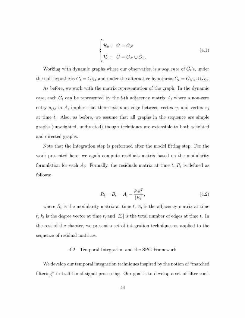
H0 : G = GN
H1 : G = GN ∪GS.
(4.1)
Working with dynamic graphs where our observation is a sequence of Gt’s, under
the null hypothesis Gt = GN,t and under the alternative hypothesis Gt = GN,t ∪GS,t.
As before, we work with the matrix representation of the graph. In the dynamic
case, each Gt can be represented by the t-th adjacency matrix At where a non-zero
entry aij,t in At implies that there exists an edge between vertex vi and vertex vj
at time t. Also, as before, we assume that all graphs in the sequence are simple
graphs (unweighted, undirected) though techniques are extensible to both weighted
and directed graphs.
Note that the integration step is performed after the model fitting step. For the
work presented here, we again compute residuals matrix based on the modularity
formulation for each At. Formally, the residuals matrix at time t, Rt is defined as
follows:
Rt = Bt = At −ktk
Tt
|Et|, (4.2)
where Bt is the modularity matrix at time t, At is the adjacency matrix at time
t, kt is the degree vector at time t, and |Et| is the total number of edges at time t. In
the rest of the chapter, we present a set of integration techniques as applied to the
sequence of residual matrices.
4.2 Temporal Integration and the SPG Framework
We develop our temporal integration techniques inspired by the notion of “matched
filtering” in traditional signal processing. Our goal is to develop a set of filter coef-
44

ficients that would amplify the strength of the signal subgraph. We apply this set
of coefficients to a time series of residual matrices as defined in Equation 4.2. This
allows us to demonstrate a novel methodology for analysis of dynamic graphs, specif-
ically, filtering for network sequences. This approach not only allows for analysis
of dynamic graphs, but also provides a significant improvement in detection perfor-
mance over the same statistical test used in the static case, enabling the detection of
significantly weaker signal subgraphs.
Working with a sequence of residual matrices where Rt represents the residuals at
time t, we integrate the residuals over a time window. Letting ` be the length of the
time window, we use a finite impulse response filter h to integrate the residuals over
time, obtaining
Rt =`−1∑i=0
Rt−ihi.
The matrix Rt is then an aggregated residuals matrix for the graph at time t. Since
our goal is detection with no cue to the subgraph vertices, we filter the modularity
matrices in their entirety, without biasing toward or requiring any a priori knowledge
with regards to any part of the graph. (Ordering of the vertices may be arbitrary, but
must be consistent within the time window.) As a result, Rt is a matrix in which each
entry is the result of a pair of vertices having its modularity filtered by h. Following
the construction of R, the rest of the algorithmic steps are applied as in the static
case as described in Chapter 3.
The challenge is to choose filter coefficients that emphasize the subgraph and
de-emphasize the background. Consider a case where a subgraph connectivity gets
increasingly denser with time. This could, for example, occur if a group of individuals
that is loosely connected started increasing its connectivity through a joint activity. In
that case, it would make sense to define a filter that is consistent with a densification
45

pattern, specifically, a filter with coefficients that increase linearly over time. Let
us consider a simulated example where a 1024 vertex background graph is generated
using the RMAT Kronecker graph generator with an average degree of each vertex
of approximately 12. In this example, the same generator is used to generate a
background graph with the same RMAT parameters for 32 time samples. For the
embedding, we create a 12 vertex subgraph with no edges at the beginning of the
time period and linearly increasing density with each time period. To detect this
subgraph, we define the following filter, h:
ht = 1− t/31, 0 ≤ t < 32
ht = ht − 1/2, (4.3)
where the subtraction of the mean intuitively de-emphasizes the background, since
the background is generated independently at each time step.
The ROC performance of applying this filter to detect a densifying subgraph is
presented in Figure 4.2. The test statistic applied here was the same chi-squared
test maximized over rotation in the plane on Rt performed on R in Section 3.4 to
determine whether H0 or H1 is true. The various lines in the figure represent varying
final density of the embedded signal subgraph. As can be observed, the detection
performance is radically improved by adding a temporal integration step leading
to near perfect detection performance for a 45% dense subgraph as compared to
effectively no better than chance performance for a 70% dense subgraph using the
static techniques as demonstrated in Figure 3.6b in Chapter 3.
46

Figure 4.2: Ramp Filter Performance as Discussed in Miller et al. (2011). Different
lines represent different final subgraph densities - the density of the embedded signal
subgraph at the last time step. The detection performance is near perfect for a
subgraph with a final density of 45%. This is significant performance improvement
over static detection algorithm where even a subgraph with 70% density was virtually
undetectable as shown in Figure 3.6b
47

4.3 Filter Optimization
In the previous section, we formulated the temporal integration for dynamic graphs
as applied to the residuals matrices. We also demonstrated the application of a ramp
filter applied to detection of a densifying subgraph. Here, we present more generally a
set of techniques to optimize the filter coefficients as described in Miller et al. (2011)
and Miller and Bliss (2012b) and applied in context of collaboration networks case
study in Chapter 6.
The goal of filter optimization is to emphasize the signal subgraph strength while
minimizing the power of the background or noise graph. As a measure of signal
strength, we use the spectral norm of the principal submatrix of Rt associated with
the subgraph, denoted by RS,t. Likewise for noise power, we can use the norm of
the modularity matrix of the background alone, denoted by RN,t. Our objective is to
maximize the former quantity while restricting the latter, which can be formulated
as
arg maxh
∥∥∥∑`−1i=0 RS(t− i)h(i)
∥∥∥subject to
∥∥∥∑`−1i=0 RN(t− i)h(i)
∥∥∥ ≤ p,(4.4)
where p is the threshold for power of the background that is set to an arbitrary
positive value. The intuition behind this is that maximizing the “power” of the
submatrix associated with the signal will help to separate it in the space of the
principal eigenvectors, which will increase the test statistic. We assume, however,
that we do not know the signal graph exactly; we only have some high-level notion of
how it evolves over time. Rather than truly solving (4.4), therefore, we use a heuristic
based on this assumption. We let h track the maximum eigenvalue of the adjacency
matrix of the subgraph alone (i.e., h(i) is the maximum eigenvalue of the subgraph’s
48

adjacency matrix at time n − i). In an ideal case where the principal eigenvector of
RS,t is constant, this will maximize the integrated signal power. Note that in the ramp
filter construction example as defined in Section 4.2, the ramp filter approximately
tracks the maximum eigenvalue of a randomly densifying graph.
The optimization discussion above assumes that we only have a notion of how
the signal evolves over time as opposed to having a known signal. If our signal is
known, we can further optimize our filter construction. In particular, here we focus
on detection of a known signal in independent, identically distributed (i.i.d.) noise.
The noise consists of i.i.d. Bernoulli graphs, meaning graphs where edges occur based
on the outcome of independent Bernoulli trials. The probabilities are not identical
across all pairs of vertices—as in Erdos–Renyi random graphs—but at each individual
time step the probability of an edge between vertex i and vertex j is the same, denoted
pij = pji. Thus, under H0, the expected value of the adjacency matrix of the graph
at any time instance, E [At], is given by P = {pij}, a |V | × |V | matrix of edge
probabilities.
Under H1, a dynamic subgraph that is unlikely to appear under H0 is embedded
into the background on a randomly selected subset of the vertices, VS ⊂ V . In this
formulation, we know the subgraph’s temporal evolution pattern, but do not know its
location in the background. While this could potentially be solved by a brute-force
search, such an approach would be a form of the subgraph isomorphism problem,
which is known to be NP-hard, or the hardest computational class of problems.
As a metric of signal and noise power, we use the spectral norm, i.e., the absolute
value of the largest eigenvalue, denoted by ‖ · ‖. To best detect the presence of the
anomalous subgraph, our goal is to maximize signal power while restricting noise
power, that is, to use coefficients
49

h∗ = arg maxh
∥∥∥∥∥L−1∑i=0
AS,t−ihi
∥∥∥∥∥ (4.5)
subject to
∥∥∥∥∥L−1∑i=0
(AN,t − E[AN,t)])hi
∥∥∥∥∥ = η.
Here AS,t is the |VS| × |VS| adjacency matrix of the dynamic foreground only, and
AN,t is the adjacency matrix of the background or noise alone. We now focus on
coefficient optimization in this problem setting.
To restrict the noise power after integration, we use the property that
‖Rt‖ = max‖u‖2=1
∣∣∣uT Btu∣∣∣ . (4.6)
Rather than truly limit the maximum eigenvalue, we will restrict the variance of Rt in
any 1-dimensional subspace of R|V |. The analysis in this section assumes knowledge
of the probability matrix P . We will analyze the moments of the quantity uT Btu,
and assume an arbitrary, fixed u of unit magnitude. The first, simple observation is
that, since Rt is a random variable minus its expected value, E[uT Rtu
]= 0, i.e.,
the distribution of uT Rtu is centered at the origin. The second-order moment of this
quantity is given by (as in Miller and Bliss (2012b))
50

E
[(uT Rtu
)2]= E
(L−1∑i=0
uT (AN,t−i − P )uhi
)2
= E
[L−1∑i=0
uTRt−iuhi
L−1∑j=0
uTRt−juhj
]
=L−1∑i=0
h2iE[(uTRt−iu
)2]
=L−1∑i=0
h2iE
|V |∑j=1
|V |∑k=1
ujuk(ajk,t−i − pjk)
2=
L−1∑i=0
h2i
[∑j,k
2u2ju2kE[(ajk − pjk)2
]−∑j
u4jE[(ajj − pjj)2
]]
=L−1∑i=0
h2i
[∑j,k
2u2ju2k(pjk − p2jk)−
∑j
u4j(pjj − p2jj)
]. (4.7)
Regardless of the direction of u, the variance of uT Rtu scales linearly with the
sum of the squares of the filter coefficients. To restrict the expected noise power,
therefore, we will fix the `2 norm of the vector of filter coefficients to be 1.
Next, we determine coefficients that solve the optimization problem as stated in
equation (4.6), and consider two other formulations. As discussed above, we restrict
the noise by setting∑L−1
i=0 h2i = 1, so the focus is on finding
h∗ = arg maxh:‖h‖2=1
∥∥∥∥∥L−1∑i=0
AS,t−ihi
∥∥∥∥∥ . (4.8)
This can be rewritten as
h∗ = arg maxh:‖h‖2=1
max‖u‖=1
L−1∑i=0
hiuTAS,t−iu. (4.9)
Let A be a 3-way tensor in which A(i, j, k) contains the value from the jth row
and kth column of AS,t−i. For symmetric (undirected) subgraphs, (4.9) is equivalent
51

to maximizingL−1∑i=0
|V |∑j=1
|V |∑k=1
A(i, j, k)hiujwk,
with the `2 norms of h, u and w all constrained to be 1. This can be solved by
finding the rank-1 approximation of A, i.e., to compute h, u and w, and a scalar λ,
such that
A ≈ λ(h ◦ u ◦ w),
where ◦ denotes the 3-way tensor outer product, with the (i, j, k)th entry of h◦u◦w
equal to hiujwk. This is analogous to approximating a matrix M by the scaled outer
product of its principal left and right singular vectors u and w, which also maximizes
the quantity uTMw =∑
i
∑jmijuiwj. We can, thus, solve (4.8) by computing
the rank-1 tensor approximation of A and use the resulting vector h as the filter
coefficients.
In Miller et al. (2011) and as described above, the filter coefficients used were
proportional to the largest eigenvalues (in magnitude) of the associated adjacency
matrices, i.e., the instantaneous signal power. While this provided adequate integra-
tion gain in the simulations, it is only the optimal solution for (4.8) when the principal
eigenvector of AS,t is constant across t.
Finally, if the task requires not only detection of anomalous activity but also iden-
tification and localization, i.e., determining which vertices are exhibiting the activity
of interest, then maximizing the largest eigenvalue may not be optimal. In this case,
it may be ideal to emphasize the cross section of the integrated residuals space that
points equally in the direction of all subgraph vertices. To do this, we maximize the
quantity
52
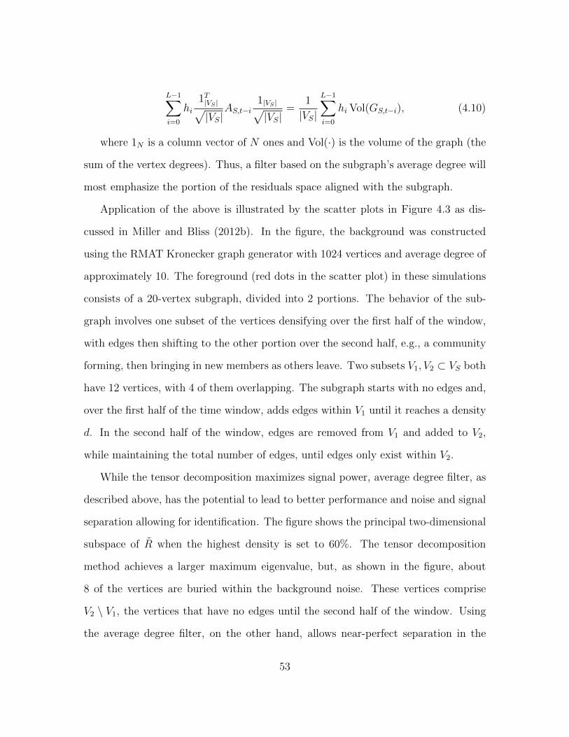
L−1∑i=0
hi1T|VS |√|VS|
AS,t−i1|VS |√|VS|
=1
|VS|
L−1∑i=0
hi Vol(GS,t−i), (4.10)
where 1N is a column vector of N ones and Vol(·) is the volume of the graph (the
sum of the vertex degrees). Thus, a filter based on the subgraph’s average degree will
most emphasize the portion of the residuals space aligned with the subgraph.
Application of the above is illustrated by the scatter plots in Figure 4.3 as dis-
cussed in Miller and Bliss (2012b). In the figure, the background was constructed
using the RMAT Kronecker graph generator with 1024 vertices and average degree of
approximately 10. The foreground (red dots in the scatter plot) in these simulations
consists of a 20-vertex subgraph, divided into 2 portions. The behavior of the sub-
graph involves one subset of the vertices densifying over the first half of the window,
with edges then shifting to the other portion over the second half, e.g., a community
forming, then bringing in new members as others leave. Two subsets V1, V2 ⊂ VS both
have 12 vertices, with 4 of them overlapping. The subgraph starts with no edges and,
over the first half of the time window, adds edges within V1 until it reaches a density
d. In the second half of the window, edges are removed from V1 and added to V2,
while maintaining the total number of edges, until edges only exist within V2.
While the tensor decomposition maximizes signal power, average degree filter, as
described above, has the potential to lead to better performance and noise and signal
separation allowing for identification. The figure shows the principal two-dimensional
subspace of R when the highest density is set to 60%. The tensor decomposition
method achieves a larger maximum eigenvalue, but, as shown in the figure, about
8 of the vertices are buried within the background noise. These vertices comprise
V2 \ V1, the vertices that have no edges until the second half of the window. Using
the average degree filter, on the other hand, allows near-perfect separation in the
53

(a)
(b)
Figure 4.3: Scatterplots of the Top Two Eigenvectors of R as Discussed in Miller
and Bliss (2012b). The tensor decomposition as illustrated in Figure 4.3a technique
used to optimize filter coefficients produces the largest signal power in context of the
detection problem. However, a number of there vertices associated with the signal
subgraph are not separated from the background vertices (signal vertices are red,
background vertices are blue). The separation on the scatter plot is improved by
applying the average degree filter as is illustrated in Figure 4.3b.
first eigenvector. Since empirical detection performance between these methods is
extremely similar, it is possible that an average degree filter would be preferable in
some situations.
54

The temporal integration and filter optimization techniques described here are ap-
plied to the case study of detecting innovation in collaboration networks as described
in Chapter 5 and results are presented in Chapter 6.
55

Chapter 5
CASE STUDY: DETECTING INNOVATION IN COLLABORATION
NETWORKS
A key element of the research is the application of the mathematical techniques
within the signal processing for graphs framework in context of a truly inter-disciplinary
approach to detection of innovation in scientific publications. Understanding scientific
innovation and how it emerges has significant implications for academic, government,
and private organizations. Unlocking the mathematical formula for innovation talks
to the fundamental understanding of knowledge. An important observation is that
the use of mathematical techniques described here does not eliminate the need to
study innovation from a historical perspective. Instead, it compliments the tradi-
tional history of science approach and allows for leveraging of the domain expertise
in a novel and potentially transformative computational environment.
Furthermore, a fundamental challenge in developing a signal processing for graphs
framework is the lack of known truth as to both noise and signal formalisms in context
of wide range of graph-based data and, in particular, in context of social networks.
Unlike traditional signal processing, where well defined physics principles guide the
fundamentals, those formalisms are absent from study of interactions of humans at
scale. While many open ended questions and future research directions remain, the
interdisciplinary approach described here allows us to make progress along these lines
and further elucidates additional directions of study.
The mathematical techniques were applied to the field of developmental and evo-
lutionary biology, specifically, to the collaboration networks of co-authors. This par-
ticular field of study was chosen as the application due to the fact that it has been
56

extensively studied and has gone through significant transformation with emergence
of the topic of gene regulatory networks. This allows for baseline validation of the
techniques and provides insight into patterns of innovation from historical perspec-
tive. The rest of the chapter describes the specific period of innovation, the analysis
that was used to generate the truth to allow for validation, and describes the dataset
under analysis, along with the networks that were constructed from the dataset.
5.1 Innovation in the Field of Evolutionary Biology
In current scientific discourse, gene regulatory networks are considered the main
explanatory concepts in evolutionary and developmental biology. This, however, was
not the case as recently as the the 1960s. Over the last five decades, evolutionary
biology has undergone several transformations including integration of systems biol-
ogy and developmental biology into evolutionary theory. In comparison, traditional
evolutionary biology is a population based theory, focusing on adaptive dynamics
of populations as primary explanation for phenotypic evolution with developmental
mechanisms playing a secondary role. In contrast, the scientific shift and an alterna-
tive trajectory builds on the fact that organisms are complex systems of genes and
gene networks and these interactions between genes have great significance in how we
evolve as a species - focusing on mechanistic explanation of development of evolution
as primary. The distinct transformation of the research field can be tied to a 1969
paper by Britten and Davidson (BD paper). Up until that paper, while the concept
of a gene and genes themselves were considered a significant actor in evolution by
Darwin, Boveri, Kuhn, and others, the notion of complex gene regulatory networks
and their influence was not considered fundamental to the concept of evolution.
57

In 1969, the BD paper introduced the notion of a regulatory network controlling
gene expression. This paper is considered to be a known innovation and disruption
in evolutionary and developmental biology leading to the fact that gene regulatory
networks are now widely considered one of the main explanatory concepts in today’s
evolutionary and developmental biology as discussed in Davidson (2010), Krakauer
et al. (2011), Laubichler et al. (2013). Furthermore, the history of this idea is also
understood, at least in its broad patterns according to Laubichler and Maienschein
(2013). This includes early conceptual ideas, dating back to the beginning of the
20th century, as well as more recent developments that derive from a clear conceptual
formulation by Roy Britten and Eric Davidson published in Science in 1969 Britten
and Davidson (1969). The Britten-Davidson (BD) model for gene regulation in higher
cells is, by all possible metrics, a case of a scientific innovation.
Detailed historical analysis of the BD paper and the model described therein has
been analyzed to reveal several interesting patterns. One of the observed patterns
in this case study is that scientific innovation leads to restructuring or rewiring of
collaborations within areas of science. This re-structuring can be directly studied
in context of co-authorship networks and thus presents a well-suited case study for
application of the signal processing for graphs techniques.
In addition to historical analysis, the impact can be shown quantitatively through
citation data. Figures 5.1 and 5.2 shows the direct and second order citations to the
BD paper. Second order citations are citations to papers that cite the BD paper and
are a good approximation for broader impacts of a scientific idea, especially when
considered together with direct citations.
As illustrated in Figures 5.1 and 5.2, direct citations to the BD paper can be
seen starting in 1969, the year of publication. From then, until 1975 the citations
continually increase reaching almost 90 per year (Figure 5.1). There is a decrease of
58

citations in the 1990s with a resurgence in citations starting in 2000s. The resurgence
in citation rates indicates a lasting impact of the paper on the scientific field as can
be observed even more prominently in the second order citations (or papers that cite
papers that cited the BD paper directly). Figure 5.2 shows the secondary citations.
Both the magnitude of the citations (reaching beyond 3000 per year) and the clear
second increase in citations in 2000s further illustrates the significance of the paper.
In the next section, we describe how we leverage the citation data as truth in context
of graph analysis.
5.2 Dataset and Collaboration Networks
In the previous section, we have described a well-known case study of scientific
innovation in the fields of evolutionary and developmental biology. Here, we dis-
cuss the specific dataset under study and the process of graph construction both of
the field collaboration networks and the “truth” networks that were used to define
the signature properties of innovation in context of the signal processing for graphs
framework described in Chapter 3 and the algorithms for analysis of dynamic graphs
in Chapter 4. As discussed earlier, at the core of the SPG framework is the notion
of signal detection within graphs - to that end, the dataset under study contains
both the background/noise data and a signal (in this case, the collaboration networks
created around the BD paper).
Large scale publication datasets, such as the ones of interest here, are well suited
to graph-theoretic analysis. As previously described, a graph is simply a mathe-
matical construct that allows us to capture both entities (vertices) and relationships
(edges) between those entities. Figure 5.3 presents two possible graphs that could be
constructed from publication data - a co-authorship graph (on the left) and a citation
graph (on the right). In a co-authorship graph, the vertices are authors and the edges
59

Figure 5.1: Britten-Davidson Citation Data - Direct Citations. The paper published
in 1969 by Roy J. Britten and Eric H. Davidson (BD) titled “Gene regulation for
higher cells: a theory” is widely considered transformative and a case study of scien-
tific innovation in the fields of evolutionary and developmental biology. This figure
and Figure 5.2 present quantitative data on citations to the BD paper illustrating
the scientific impact. This figure presents direct citations to the paper. Together,
both figures support the scientific impact of the paper in terms of number of citations
and lasting impact of citations, with a resurgence of paper’s popularity in 2000s as
illustrated by direct and second order citations.
60

Britten and Davidson 1969 Secondary Citation History
Figure 5.2: Britten-Davidson Citation Data - Secondary Citations. This figure
presents the secondary citations - citations to the papers that cite the BD paper
directly.
represent a “co-author” relationship as indicated by a particular publication (authors
appearing formally on the same publication. Note that the co-author relationship
is undirected. These graphs could be weighted with weights representing number of
times two authors have published together. In a citation graph, traditionally, the
vertices are papers (though they could also be authors of those papers) and the edges
represent a “cited” relationship - an edge between paper i and paper j indicates that
paper i cited paper j. Note that unlike co-authorship networks, citation networks are
unweighted (a paper is only going to cite another paper once) and directed (the cita-
tion relationship has directionality). Other graphs are possible as well, such graphs
based on keywords in the papers - for example, vertices could represent papers and
edges represent a “sharing of keywords” relationship.
61

Author'A2'and'Author'A3'have'co0authored'a'paper'together'
A1' A2'
A3' A4'
A5'
P1'
P2'P3'
P4'
Paper'P4'cites'Paper'P1'
Figure 5.3: Illustration of Co-Authorship and Citation Graphs.
As the goal of the analysis is to detect emerging collaborations, we focus here
on co-authorship graphs. Additionally, co-authorship graphs do indeed provide good
representation of collaboration relationship.
Formally, the co-authorship graph, G = (V,E), represents a set of authors, V that
are connected by an edge E if vi and vj have published together. These graphs are
naturally dynamic, as publications have dates, and thus, a sequence of graphs can
be used to represent co-authorship relationships over time, with G(n) representing
authors that publish together at time n, where each G(n) represents a publication
year.
5.2.1 Background Graph
We construct the background graph from the publication data of the entire field
of developmental biology as constructed by the Laubichler Lab at ASU. The source of
62

the publication data is the Thompson Reuters Web of Science database. Web of Sci-
ence (WoS) is a commercially available research database of papers in the sciences,
social sciences, arts, and humanities. The full database has more than 42 million
records from 1900 to the present and includes articles from over 12,000 journals and
148,000 conference proceedings. Records in WoS typically include author(s), title,
publication date, type, document IDs for works cited, and may also include subject
area, institution, keywords, and abstract as provided by the publication. Some addi-
tional work on this dataset is covered in B. A. Miller et al. (2012), B. A. Miller et al.
(2013), and Miller et al. (2013a) technical report.
The developmental biology portion of the WoS data covers the top 12 journals in
developmental biology, Science, Nature, and the Proceedings of the National Academy
of Sciences (PNAS). The years covered by our analyses are 1969 (publication of the
BD paper) to 2000. In constructing the background graph, the number of unique
authors was held consistently to 294,700 as that was the total number of authors under
consideration during the period of interest. The ordering of the authors in the graph,
while arbitrary, was preserved as is necessary for each year. As described above, G(n)
represents the co-authorship graph from a given year, n in the period of 1969-2000.
For each year, the graphs constructed were both unweighted and undirected. The
scale of this graph is significant where traditional traversal-based analysis techniques
encounter computational challenges, but is well suited to the SPG framework and
the tractability of techniques within it. A sample of raw data is provided in Table
5.1. Each line represents a co-authorship relationship - the first two entries in a given
line identify the vertex end points of each edge. The last entry is the weight of an
edge. Note that while two authors may have published together multiple times, thus
resulting in a edge weight greater than 1, for analysis purposes all edge weights were
converted to 1.
63

Table 5.1: Sample of Raw Data - 1969 Co-Authors
Index of Vertex (Author) 1 Index of Vertex (Author) 2 Edge Weight
... ... ...
8 287732 1
18 149619 1
18 157955 1
18 229956 1
108 102728 1
108 241053 1
141 3141 1
... ... ...
5.2.2 Signal Graph
The signal graph was constructed using the citation data (also extracted from the
Web of Science database), specifically direct citations to the BD paper as illustrated
in Figure 5.1 to identify the authors that are part of the signal graph. For each year
n, GS(n) contained authors that cited the BD paper as vertices with an existence
of an edge between two vertices indicating that two authors co-authored a paper
together. While the nature of a citation could vary, given the scale of this analysis,
this approach is relevant to allow for tracking of trends in re-wiring of collaboration
networks.
The signal graph was constructed for the period of 1969-1980, focusing on the
period of emergence of the BD model and its influence. Figure 5.4 presents an ex-
64

ample signal subgraph for the year 1975. Results of the application of techniques are
presented in the next chapter.
65
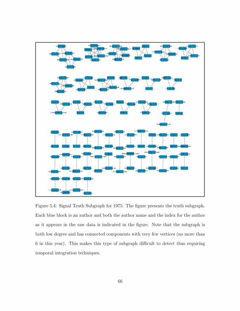
Figure 5.4: Signal Truth Subgraph for 1975. The figure presents the truth subgraph.
Each blue block is an author and both the author name and the index for the author
as it appears in the raw data is indicated in the figure. Note that the subgraph is
both low degree and has connected components with very few vertices (no more than
6 in this year). This makes this type of subgraph difficult to detect thus requiring
temporal integration techniques.
66
Chapter 6
RESULTS
In this chapter we present results of applying the techniques described in Chapter
3 and Chapter 4 to the known case study of scientific innovation in developmental
biology discussed in Chapter 5 and as described in Bliss et al. (2014b), Miller et al.
(2015). We predominantly focus on analysis of dynamic networks to gain insight
into the structure of transformative events in science and impact of innovation on
collaboration networks. Bettencourt et al. (2009) discusses alternative approaches to
analysis of innovation in context of collaboration networks leveraging graph theoretic
measures such as density, diameter, and connected component analysis as opposed to
detection of signals.
As described in Chapter 5, our data is well-suited to graph-theoretic analysis.
The input into the SPG framework is a graph G or a time series of graphs, with no
vertex cue, as represented by the adjacency matrix where aij is non-zero if an edge
exists between vertex vi and vj in G. All graphs analyzed here are unweighted and
undirected and have 294,700 vertices as that is the number of unique authors in the
primary time period under analysis, spanning 1969-2000.
For each of the results discussed below, we also highlight the relevant algorithmic
blocks in the SPG block diagram to indicate which mathematical techniques were
applied.
6.1 Evolution of the Scientific Field
Before focusing on detection of the signature of innovation, we are first inter-
ested in understanding whether our mathematical techniques can provide insight into
67

INTEGRATION MATRIX DECOMPOSITION
COMPONENT SELECTION
ANOMALY DETECTION IDENTIFICATION MODEL FITTING
DIMENSIONALITY REDUCTION
Figure 6.1: SPG Block Diagram - Evolution of the Scientific Field Relevant Blocks. To
consider the impact on the overall scientific field, we applied to model fitting/residual
computation step and the dimensionality reduction step to an ensemble of years in
the period under study.
general evolution of the scientific field. Given that the BD paper is a well-accepted
disruptor in evolutionary and developmental biology, our first application was to con-
sider the two dimensional projections of an ensemble of years throughout the period
under study. Figure 6.1 highlights the relevant algorithmic blocks.
To perform this analysis, we analyzed static co-authorship graphs for a number of
years, performing the residual computation on each, followed by an eigendecomposi-
tion and projection of the data into the space of the top two eigenvectors as described
in Chapter 3. The modularity matrix B = A−kkT/M was used for the residual com-
putation. A set of projections for representative years is shown in Figure 6.2. We
expanded our analyses to years prior to the publication of the BD paper (1959) to
further study the impact. The years were chosen to highlight the field before the BD
paper (1959), publication year of the BD paper (1969), near to mid term impact of
the BD paper (1989), and long term impact of the BD paper (1999).
In each of the subplots in the figure, individual dots represent vertices in the
graph or individual authors. The axes are the values corresponding to each vertex in
eigenvectors 1 and 2 (the eigenvectors associated with the two largest eigenvalues).
The shape of the projection is clearly evolving over the course of the decades under
study and is consistent with the historical data, providing initial validation of the
68

Eig
enve
ctor
2
Eig
enve
ctor
2
Eigenvector 1
Eigenvector 1
Eigenvector 1
Eigenvector 1
Eig
enve
ctor
2
Eig
enve
ctor
2
Figure 6.2: SPG Analysis of the Field of Developmental Biology. For each year, we
performed the residual computation (model fitting) and the dimensionality reduction
step. This analysis does not perform any temporal integration. The figure presents
a two-dimensional projection of the co-author network with each point on the plot
representing a single vertex (author).
69

suitability and sensitivity of the techniques for the topic of interest - detection of
innovation in collaboration networks.
The historical study of the scientific field validates the results achieved via the
graph-theoretic analysis. During the 1960s and 1970s the field was still relatively
diverse. In 1979 the majority of genetic work in developmental biology focused on
single genes. What we see in the progression of graphs is the (1) the constancy
of genetic approaches (2) the emergence of some (short-lived) fashions and (3) the
subsequent expansion and diversification of genetic and genomic approaches. By the
1980s and 1990s, the field coheres around a single theme.
6.2 Author Detection
In this section, we describe a number of experiments leveraging the techniques for
dynamic graphs as presented in Chapter 4. First, we present results of applying two
different types of filters to a known period of innovation. We then present techniques
for additional filter optimization, highlighting some of the relevant results as described
in Miller et al. (2015). Finally, we demonstrate the application of one of the filters to a
different time period, indicating that innovation may have generalizable collaboration
network patterns. The block diagram highlighting the relevant blocks of the SPG
framework is presented in Figure 6.3. Since the focus of the research is the temporal
integration in collaboration networks, that block is further highlighted. Note that we
skip the anomaly detection step in these experiments as we have a priori knowledge
as to existence of innovation in scientific publications during the period under study.
6.2.1 Dynamic Integration of Collaboration Networks
Here we present an application of two dynamic integration techniques to temporally-
evolving collaboration networks. As previously described, the input into the SPG
70

INTEGRATION MATRIX DECOMPOSITION
COMPONENT SELECTION
ANOMALY DETECTION IDENTIFICATION MODEL FITTING
DIMENSIONALITY REDUCTION
Figure 6.3: SPG Block Diagram - Author Detection Relevant Blocks. To identify key
author subgraphs, we applied the model fitting/residual computation step, temporal
integration step, dimensionality reduction step, and identification step to a dynamic,
temporally evolving collaboration network. Since the focus of the work presented is
the temporal integration, that algorithmic block is further highlighted.
framework is a time series of adjacency matrices, with each time slice representing
the collaboration network for a given year. For each adjacency matrix in the time
series, aij is non-zero if author i and author j have published together in a given
year. Our techniques here were applied to the years 1969-1980. Note also, that those
were the years for which we have constructed the signal subgraphs based on truth
citation history and associated collaborations. Furthermore, the truth subgraphs are,
as would be expected, part of the overall input graph - the collaborations identified
as relevant to the BD transformation naturally exist in the background of the entire
field.
We first applied a ramp filter, or filter of linearly increasing coefficients, to the
time series data as indicated by the equation:
Rn =T−1∑t=0
R(n−t)ht. (6.1)
Where Rn is the residuals matrix at time n and h is a vector of filter coefficients,
and T is the length of the time series. A ramp filter (linearly increasing coefficients)
has the ability to increase the signal of a densifying connectivity pattern. A ramp
71

filter is constructed by creating filter coefficients that increase over time, centered,
and normalized (T here is still the length of the time window of interest):
h′t = t− T/2 (6.2)
h = h′/ ‖ h′ ‖ (6.3)
A change in a scientific field potentially could exhibit such a pattern - for example,
increasing set of collaborations between groups of loosely connected researchers.
Recall, that the signal subgraph for each of the years spanning 1969-1980 was
constructed based on collaborations between authors that have sighted the BD paper.
For each of the years, we computed the eigenvalues of the truth subgraph and have
constructed our normalized coefficient vector h based on the maximum eigenvalue,
λmax, of that subgraph for each year.
Results for both the ramp filter and filter tracking the maximum eigenvalue of the
signal (the truth data) are presented in Figure 6.4. As with the results in the previous
section, we present the two-dimensional projections of the temporally integrated dy-
namic collaboration network. As we have the truth data of the subgraphs of interest
(as identified by the citations), we can highlight those vertices in red. Each point, as
before, represents a vertex in the graph or an author.
A few observations can be readily made from these results. It is apparent from
the analysis that the ramp filter does not lead to any separation of the signal vertices
- as can be seen in the left-hand plot in Figure 6.4, they are entirely hidden within the
center of the background. On the other hand, the maximum eigenvalue filter clearly
identified the author Monroy, A. Alberto Monroy was a leading figure in Italian and
European developmental biology. Monroy was one of the first prominent developmen-
tal biologist, who applied the new concept of gene regulatory networks in the context
72

Monroy, A
Eigenvector 1 Eigenvector 1
Eig
enve
ctor
2
Eig
enve
ctor
2
Figure 6.4: Temporal Integration Leveraging Truth. Two filters were applied: a
ramp filter and a maximum eigenvalue of the truth subgraph filter. The red colored
points indicated the known truth data (based on the GS subgraph). As in Figure
6.2, each point represents an author in the co-author network. The ramp filter does
not separate the truth from the background. The maximum eigenvalue filter does
identify a key individual, Monroy A.
of molecular explanations of developmental processes in the mid-1970s. These results
are also consistent with the historical observations that innovation causes a re-wiring
of the collaboration networks (as opposed to densification).
6.2.2 Filter Optimization
While the results obtained using the λmax-optimized filter are highly promising,
here we present some possible optimizations to the temporal integration approach as
discussed in Miller et al. (2015).
Within the SPG framework, the spectral norm is a good power metric for signal
and noise power as discussed in Miller et al. (2014). When an embedded subgraph’s
spectral norm is large, its vertices are more likely to stand out in the eigenspace.
73

When working with the temporal integration technique described in Chapter 4, this
means that it is desirable to choose filter coefficients that maximize the spectral norm
of the principal submatrix of the adjacency matrix associated with the signal subgraph
vertices.
As originally discussed in Miller and Bliss (2012b), the subgraph’s spectral norm
can be maximized by forming a 3-way tensor from the subgraph adjacency matrix,
and computing a low-rank approximation for this tensor. Let AS be an NS ×NS × `
tensor for the subgraph vertices, where NS = |VS|. The first two dimensions represent
vertices and the third dimension represents time. Much like approximating a matrix
with its singular value decomposition, a low-rank tensor decomposition can be used
to approximate AS. For a rank-1 approximation, this is achieved by solving
arg maxλ,x,y,z
NS∑i=1
NS∑j=1
∑t=1
(AS(i, j, t)− λxiyjzt)2 (6.4)
subject to ‖x‖2 = 1, ‖y‖2 = 1, ‖z‖2 = 1.
Here x, y ∈ RNS and z ∈ R` are vectors, and λ ∈ R is a scalar. Our objective is to
maximize the spectral norm of the integrated adjacency matrix whose ijth entry is
given by
ahij =∑t=1
AS(i, j, `+ 1− t)h(t).
It turns out that this quantity is optimized—under the constraint that the squares
of the filter weights sum to 1—by setting the filter weights h(t) equal to the time-
reversed temporal factor z`+1−t from (6.4). This computation can be done in Matlab
using the PARAFAC decomposition as described in Acar et al. (2011) in the Tensor
Toolbox by Bader et al. (2012).
The effect of tuning the filter with respect to the vertices of interest has been
demonstrated in simulation Miller and Bliss (2012b), but here we demonstrate ap-
plication to the well-studied period of scientific innovation described in the previous
74

chapter: we optimize the filter applied to the coauthorship graph from 1969 to 1980.
As demonstrated in Fig. 6.5, the impact is extremely significant.
Within each plot, there is one curve for each vertex in the subgraph of interest. In
each case, the eigenvectors associated with the largest 20 (non-negative) eigenvalues
were computed. The values of the plots are the components of the (unit-normalized)
eigenvectors that are associated with the subgraph vertices. Without any knowledge
of truth, one may assume that simply averaging over time would be a reasonable
approach, or that integrating using a ramp filter as described above would detect
interesting subgraphs, given that this would emphasize emerging densifying behavior.
Using these strategies, as shown in the figure, there is only one vertex that is partic-
ularly strong within the eigenvectors with the largest eigenvalues. Using a method
that considers the spectral norm of the subgraph at each point in time (i.e., using
weights corresponding to the instantaneous power of the foreground) provides some
additional benefit, as a few additional vertices stand out more prominently in eigen-
vector 14. Using a filter that is optimized via the tensor decomposition, on the other
hand, brings out several more vertices. When this filter is applied, nine vertices from
the subgraph stand out significantly in eigenvector four. Looking back at the data
used to optimize the graph (i.e., the authors citing the seminal BD paper), these nine
vertices comprise the largest connected component in any given year, and in fact form
a clique (a graph with all possible edges) in 1977. Two of the authors in this cluster
are also part of a larger clique with nine other authors in the background, who also
stand out in the same eigenvector. This is a significant finding: the most intercon-
nected that authors citing the BD paper ever become in a given year, as well as other
close collaborators. Without this temporal integration technique, the subgraph would
not stand out from the background within this low-dimensional space.
75

0 5 10 15 20−0.05
0
0.05
0.1
0.15
Eigenvector Index
Eig
en
ve
cto
r C
om
po
ne
nt
Va
lue
Equal Weights
0 5 10 15 20−0.2
−0.1
0
0.1
0.2
0.3
0.4
Eigenvector Index
Eig
en
ve
cto
r C
om
po
ne
nt
Va
lue
Ramp Filter
0 5 10 15 20−0.2
−0.1
0
0.1
0.2
Eigenvector Index
Eig
en
ve
cto
r C
om
po
ne
nt
Va
lue
Eigenvalue−Based Filter
0 5 10 15 20−0.1
0
0.1
0.2
0.3
0.4
Eigenvector Index
Eig
en
ve
cto
r C
om
po
ne
nt
Va
lue
Optimized Filter
Figure 6.5: Projections of Subgraph Vertices onto Principal Eigenvectors with Various
Temporal Integration Techniques. Within the space of the principal eigenvectors,
only one vertex is particularly prominent when using equal weights (top left), linearly
increasing weights (top right), or weights determined by eigenvalues (bottom left).
Only when an optimized filter is applied (bottom right) do a substantial number of
subgraph vertices become prominent in the eigenspace.
76

6.2.3 Generalizing to a Later Time Period
The results presented in the two subsections above all focus on the same period
of time where the signal subgraph is known to be present and is used for both filter
construction and filter optimization. A key question of interest to the broad scien-
tific and policy community is whether there is a consistent observable or detectable
structure of innovation - effectively a mathematical formula for innovation that can
be detected in early, emergent stages, potentially encouraged, and possibly even am-
plified through investment of resources. To provide initial investigation towards that
question, we apply the λmax-optimized filter to a later time period in the developmen-
tal biology dataset. Specifically, we are interested in the question as to whether a filter
constructed over a period of time from 1969-1980, leveraging known truth based on
co-authorship networks constructed around citations to the BD paper can be applied
to a different time period (1990-2000) and identify interesting individuals. Given that
this is still considering the developmental biology discipline and a well-studied period
from a historical perspective, we can perform this experiment and validate our results.
The results of the two dimensional projection are shown in Figure 6.6. A simple
thresholding procedure (analogous to a one dimensional clustering) produces 4 names:
(1)Voet, M, (2) Sprincl, L, (3) Mewes, HW, and (4) Murphy, L. From a history of
science perspective, Hans-Werner Mewes is a significant figure in this context. Mewes
has been an early proponent of Systems Biology. One of the conceptual consequences
of the notion of gene regulatory networks is a shift away from a single gene to a
genomic network paradigm, so it is not at all surprising that we detect proponents of
Systems Biology within the innovation trajectory of the Britten-Davidson paper.
The results are highly promising illustrating both the efficacy of the approach and
the need for interdisciplinary techniques - in this case bringing together the graph
77

Eigenvector 1
Eig
enve
ctor
2
Figure 6.6: Temporal Integration on a New Time Period. As in Figure 6.2, each
point represents an author in the co-author network. The maximum eigenvalue filter
constructed leveraging truth data covering the 1969-1980 time period is applied to
a new time window: 1980-2000. The SPG approach with a truth-based filter and a
simple thresholding procedure identifies 4 individuals, one of which is considered a
significant figure in scientific innovation in developmental biology, Mewes, HW.
78

theoretic and history of science domains. Furthermore, the scalability of the tech-
niques makes this approach highly applicable to wide range of scientific collaboration
datasets, allowing us to detect and potentially formulate general attributes of inno-
vation.
79
Chapter 7
CONCLUSION
In this dissertation, we presented a novel algorithmic framework for detection of
small, topologically anomalous subgraphs in large graph datasets and applied the
framework to a case study of detection of innovation in collaboration networks lever-
aging rigorously studied periods in history of science. Both the framework formulation
(including the notion of signal processing for graphs) and its application constitute
novel contributions to the field of applied mathematics, particularly in the context
of life and social sciences and humanities. These techniques have significant poten-
tial to greatly improve understanding and detecting of emergence of new concepts in
science. Both simulated results and application results presented here demonstrate
the potential of the approach to transform our understanding of complex systems
created by social networks in context of scientific research. The SPG framework
facilitates specialization of subgraph detection algorithms for diverse, specific appli-
cation requirements, as well as various data sources, types, and scales. Furthermore,
the contributions of this work demonstrate a truly interdisciplinary approach by ad-
vancing the mathematical techniques while also advancing our understanding of the
fundamentals of knowledge.
Applying our method of signal detection to study patterns of innovation within
science leveraging rigorous historical knowledge of a transformative period in develop-
mental and evolutionary biology allowed us to (1) identify these events within graphs
of scientific collaboration and (2) validate our findings with concrete historical analy-
sis of the detected signatures. A key finding of interest is confirmation that innovation
leads to re-wiring of networks of collaboration connections and not necessarily den-
80

sification. This is directly supported by results presented in Section 6.2.1 and in
Figure 6.4. The ramp filter, tracking a densifying pattern, produced no noise/signal
separation, while the filter tracking the maximum eigenvalue of the signal subgraph
did. This result mathematically supports historical analysis of this period and is a
step towards formulating the topology or connectivity signature of innovation. This
is further confirmed by the fact that applying this same filter to a later time period
leads to similar discovery as illustrated in Figure 6.6.
The formulation of the signal processing for graphs framework as it has been
defined and instantiated in this research provides a means for identifying potential
research directions both from the perspective of development of models and techniques
and from the perspective of the application of interest - detection of emergence of
innovation. Here, we outline these future directions.
Throughout this dissertation, we leveraged the modularity matrix as our residuals
matrix. This residuals computation is based on the Chung-Lu graph model. While we
have been able to demonstrate great results both in simulation and in our case study,
it is likely that the underlying model of publication data is not in fact Chung-Lu.
Specifically, the Chung-Lu model assumes that there is no community structure in the
graph, which is explicitly not the case in context of scientific collaborations. Scientific
collaborations are defined by their community structure and it is the deviation from
existing community structure that is of interest in context of detection of scientific
innovation. Developing an expected model building on the one described in Miller and
Bliss (2012a) is likely to improve the detection performance in identifying emerging
research trends.
In Section 6.2.2, we presented a filter optimization technique to increase the power
of our signal subgraph based on a known case study. This optimization leveraged the
fact that the subgraph was exactly known and the signal strength was optimized
81

by maximizing the spectral norm of the subgraph. One potential research direction
is continued development of filter optimization techniques with varying knowledge
of the subgraph. Also, as discussed above, a better formulation of the expected
model is likely to allow for more effective noise suppression thus providing another
means to amplify the signal. Another potential area of exploration in context of
temporally evolving graphs is to consider formulation for continuos as opposed to
discrete representations presented here.
In our case study, we focused predominantly on principal component analysis of
the residuals matrix. Many additional techniques for component selection can be
considered, such as ones that were developed in Miller et al. (2010a). It would also
be interesting to consider applying the component selection techniques in context
of dynamic subgraph detection. Another potential direction is to explore higher di-
mensional representations of the graph - in all of our research, we have focused on
two-dimensional projections. It is possible that addition of extra dimensions could in-
crease detection performance, while still operating in a significantly lower dimensional
space than the original input graph.
As discussed in Section 2.1.1, the problem of subgraph isomorphism is NP-complete.
All of the SPG techniques have polynomial time complexity. It would, therefore,
be of interest to investigate theoretical performance bounds of these approximation
algorithms and explore the cases where optimal performance can be achieved in poly-
nomial time. Also, as mentioned in Chapter 2, new results from random matrix
theory are likely to be relevant in context of deriving optimal performance bounds
for subgraph detection - that would be another interesting future direction.
Finally, as we have demonstrated in both Chapter 5 and Chapter 6, applying
the mathematical techniques from the SPG framework to real data produces both
interesting mathematical results and highlights new areas to consider in context of
82

the study of innovation. We have focused our research on the case study of the
transformative nature of the Britten-Davison paper on gene regulatory networks as
it is a well-studied period of scientific innovation. A clear future direction is applying
the techniques to datasets from other disciplines both in the presence of known case
studies and in absence of those. This approach, specifically given its computational
tractability, enables studying scientific innovation at scale. Another future application
of a refined method is to observe the innovation dynamics of science closer to real
time, which would have implications for science policy, by allowing identification of
emerging scientific areas.
83

REFERENCES
Acar, E., D. M. Dunlavy and T. G. Kolda, “A scalable optimization approach forfitting canonical tensor decompositions”, Journal of Chemometrics 25, 2, 67–86(2011).
Arias-Castro, E. and N. Verzelen, “Community detection in random networks”,Preprint: arXiv.org:1302.7099 (2013).
Asahiro, Y., R. Hassin and K. Iwama, “Complexity of finding dense subgraphs”,Discrete Applied Mathematics , 121, 15–26 (2002).
B. A. Miller et al., “A scalable signal processing architecture for massive graph analy-sis”, in “Proc. IEEE Int. Conf. Acoust., Speech and Signal Process.”, pp. 5329–5332(2012).
B. A. Miller et al., “Efficient anomaly detection in dynamic, attributed graphs”, in“Proc. IEEE Intelligence and Security Informatics”, pp. 179–184 (2013).
Bader, B. W., T. G. Kolda et al., “Matlab tensor toolbox version 2.5”, Availableonline, URL http://www.sandia.gov/$\sim$tgkolda/TensorToolbox/ (2012).
Batada, N. N., T. Reguly, A. Breitkreutz, L. Boucher, B.-J. Breitkreutz, L. D. Hurstand M. Tyers, “Stratus not altocumulus: A new view of the yeast protein interac-tion network”, PLoS Biology 4, 10, 1720–1731 (2006).
Bettencourt, L. M., A. Cintron-Arias, D. I. Kaiser and C. Castillo-Chavez, “Thepower of a good idea: Quantitative modeling of the spread of ideas from epidemio-logical models”, Physica A: Statistical Mechanics and its Applications 364, 513–536(2006).
Bettencourt, L. M., D. I. Kaiser and J. Kaur, “Scientific discovery and topologicaltransitions in collaboration networks”, Journal of Informetrics 3, 3, 210–221 (2009).
Bettencourt, L. M., D. I. Kaiser, J. Kaur, C. Castillo-Chavez and D. E. Wojick,“Population modeling of the emergence and development of scientific fields”, Sci-entometrics 75, 3, 495–518 (2008).
Biggs, N., E. K. Lloyd and R. J. Wilson, Graph Theory, 1736-1936 (Clarendon Press,1986).
Bliss, N. T., A. O. Hero and B. A. Miller, “Statistical signal processing for graphs”,IEEE International Conference on Acoustics, Speech, and Signal Processing Tuto-rial, Subject Area: Fundamentals (2014a).
Bliss, N. T., B. R. E. Peirson, D. Painter and M. D. Laubichler, “Anomalous subgraphdetection in publication networks: Leveraging truth”, in “Proc. 48th AsilomarConf. Signals, Syst. and Comput.”, (2014b).
84

Britten, R. J. and E. H. Davidson, “Gene regulation for higher cells: a theory”,Science 165, 891, 349–357 (1969).
Bu, D., Y. Zhao, L. Cai, H. Xue, X. Zhu, H. Lu, J. Zhang, S. Sun, L. Ling, N. Zhang,G. Li and R. Chen, “Topological structure analysis of the protein–protein interac-tion network in budding yeast”, Nucleic Acids Research 31, 9, 2443–2450 (2003).
Chakrabarti, D. and C. Faloutsos, “Graph mining: Laws, generators, and algo-rithms”, ACM Computing Surveys 38, 1 (2006).
Chakrabarti, D., Y. Zhan and C. Faloutsos, “R-MAT: A recursive model for graphmining”, in “Proc. SIAM Int. Conf. Data Mining”, pp. 442–446 (2004).
Chang, H.-H., J. M. F. Moura, Y. L. Wu and C. Ho, “Early detection of rejection incardiac MRI: A spectral graph approach”, in “Proc. IEEE Int. Symp. BiomedicalImaging”, pp. 113–116 (2006).
Chen, K., C. Huo, Z. Zhou and H. Lu, “Unsupervised change detection in SAR imageusing graph cuts”, in “IEEE Int. Geoscience and Remote Sensing Symp.”, vol. 3,pp. 1162–1165 (2008).
Chowell, G. and C. Castillo-Chavez, “Worst-case scenarios and epidemics”, Bioter-rorism: Mathematical Modeling Applications in Homeland Security. Frontiers inApplied Mathematics 28, 35–53 (2003).
Chowell, G., J. M. Hyman, S. Eubank and C. Castillo-Chavez, “Scaling laws for themovement of people between locations in a large city”, Physical Review E 68, 6,066102 (2003).
Chung, F. and L. Lu, “The average distances in random graphs with given expecteddegrees”, Proceedings of the National Academy of Sciences 99, 25, 15879–15882(2002a).
Chung, F. and L. Lu, “Connected components in random graphs with given expecteddegree sequences”, Annals of combinatorics 6, 2, 125–145 (2002b).
Chung, F. R. K., Spectral Graph Theory (American Mathematical Society, 1997).
Coffman, T. R. and S. E. Marcus, “Pattern classification in social network analysis:A case study”, in “Proc. IEEE Aerospace Conf.”, pp. 3162–3175 (2004).
Coppersmith, G. A. and C. E. Priebe, “Vertex nomination via content and context”,Preprint: arXiv.org:1201.4118v1 (2012).
Cormen, T. H., C. E. Leiserson and R. L. Rivest, Introduction to Algorithms (MITPress, 1990).
Council, N. R., “Frontiers in massive data analysis”, (2013).
Davidson, E. H., The regulatory genome: gene regulatory networks in developmentand evolution (Academic Press, 2010).
85

Deshpande, M., M. Kuramochi, N. Wale and G. Karypis, “Frequent substructure-based approaches for classifying chemical compounds”, IEEE Trans. on Knowledgeand Data Engineering 17, 8, 1036–1050 (2005).
Ding, Q. and E. D. Kolaczyk, “A compressed PCA subspace method for anomalydetection in high-dimensional data”, IEEE Trans. Inf. Theory 59 (2013).
Du, N., B. Wu, X. Pei, B. Wang and L. Xu, “Community detection in large-scale socialnetworks”, in “Proc. ACM Int. Conf. Knowledge Discovery and Data Mining”, pp.16–25 (2007).
Easley, D. and J. Kleinberg, Networks, crowds, and markets: Reasoning about a highlyconnected world (Cambridge University Press, 2010).
Eberle, W. and L. Holder, “Anomaly detection in data represented as graphs”, Intel-ligent Data Analysis 11, 6, 663–689 (2007).
Erdos and Renyi, “On random graphs i.”, Publ. Math. Debrecen 6, 290–297 (1959).
Faloutsos, M., P. Faloutsos and C. Faloutsos, “On power-law relationships of theInternet topology”, in “Proc. SIGCOMM”, (1999).
Fasino, D. and F. Tudisco, “An algebraic analysis of the graph modularity”, Preprint:arXiv:1310.3031 (2013).
Gelbord, B., “Graphical techniques in intrusion detection systems”, in “Proc. Int.Conf. Information Networking”, pp. 253–258 (2001).
Herrera-Valdez, M. A., M. Cruz-Aponte and C. Castillo-Chavez, “Multiple outbreaksfor the same pandemic: local transportation and social distancing explain the dif-ferent waves of a-h1n1pdm cases observed in mexico during 2009”, MathematicalBiosciences and Engineering (MBE) 8, 1, 21–48 (2011).
Hirose, S., K. Yamanishi, T. Nakata and R. Fujimaki, “Network anomaly detectionbased on eigen equation compression”, in “Proc. ACM Int. Conf. Knowledge Dis-covery and Data Mining”, pp. 1185–1193 (2009).
Ide, T. and H. Kashima, “Eigenspace-based anomaly detection in computer systems”,in “Proc. ACM Int. Conf. Knowledge Discovery and Data Mining”, pp. 440–449(2004).
Kay, S. M., Fundamentals of Statistical Signal Processing, Volume II: Detection The-ory (Prentice Hall PTR, 1998).
Kleinberg, J. M., “Authoritative sources in a hyperlinked environment”, J. ACM 46,5, 604–632 (1999).
Krakauer, D. C., J. P. Collins, D. Erwin, J. C. Flack, W. Fontana, M. D. Laubich-ler, S. J. Prohaska, G. B. West and P. F. Stadler, “The challenges and scope oftheoretical biology”, Journal of theoretical biology 276, 1, 269–276 (2011).
86

Krivanek, A. and M. Sonka, “Ovarian ultrasound image analysis: Follicle segmenta-tion”, IEEE Trans. Med. Imag. 17 (1998).
Laubichler, M. and J. Maienschein, “Developmental evolution”, in “The CambridgeEncyclopedia of Darwin and Evolutionary Thought”, edited by M. Ruse, pp. 375–382 (Cambridge University Press, Cambridge, 2013).
Laubichler, M. D., J. Maienschein and J. Renn, “Computational perspectives in thehistory of science: To the memory of peter damerow”, Isis 104, 1, 119–130 (2013).
Le, T. and C. N. Hadjicostis, “Graphical inference for multiple intrusion detection”,IEEE Trans. on Information Forensics and Security 3, 3, 370–380 (2008).
Lieberman, E., C. Hauert and M. A. Nowak, “Evolutionary dynamics on graphs”,Nature , 433, 312–316 (2005).
Mifflin, T. L., C. Boner, G. A. Godfrey and J. Skokan, “A random graph model forterrorist transactions”, in “Proc. IEEE Aerospace Conf.”, pp. 3258–3264 (2004).
Miller, B. A., M. S. Beard and N. T. Bliss, “Matched filtering for subgraph detectionin dynamic networks”, in “Proc. IEEE Statistical Signal Process. Workshop”, pp.509–512 (2011).
Miller, B. A., M. S. Beard, M. D. Laubichler and N. T. Bliss, “Temporal and multi-source fusion for detection of innovation in collaboration networks”, in “Proc. Int.Conf. Inform. Fusion”, (2015).
Miller, B. A., M. S. Beard, P. J. Wolfe and N. T. Bliss, “A spectral framework foranomalous subgraph detection”, Preprint: arXiv:1401.7702 (2014).
Miller, B. A., N. Bliss, N. Arcolano, M. Beard, J. Kepner, M. Schmidt and E. Rut-ledge, “Very large graphs for information extraction (vlg): Summary of first-yearproof-of-concept study”, Lincoln Laboratory Project Report VLG-1 (2013a).
Miller, B. A. and N. T. Bliss, “A stochastic system for large network growth”, SignalProcessing Letters, IEEE 19, 6, 356–359 (2012a).
Miller, B. A. and N. T. Bliss, “Toward matched filter optimization for subgraph detec-tion in dynamic networks”, in “Proc. IEEE Statistical Signal Process. Workshop”,pp. 113–116 (2012b).
Miller, B. A., N. T. Bliss and P. J. Wolfe, “Subgraph detection using eigenvectorL1 norms”, in “Advances in Neural Inform. Process. Syst. 23”, edited by J. Laf-ferty, C. K. I. Williams, J. Shawe-Taylor, R. Zemel and A. Culotta, pp. 1633–1641(2010a).
Miller, B. A., N. T. Bliss and P. J. Wolfe, “Toward signal processing theory for graphsand non-Euclidean data”, in “Proc. IEEE Int. Conf. Acoust., Speech and SignalProcess.”, pp. 5414–5417 (2010b).
87

Miller, B. A., N. T. Bliss, P. J. Wolfe and M. S. Beard, “Detection theory for graphs”,Lincoln Laboratory J. 20, 1 (2013b).
Nadakuditi, R. R., “On hard limits of eigen-analysis based planted clique detection”,in “Proc. IEEE Statistical Signal Process. Workshop”, pp. 129–132 (2012).
Nadakuditi, R. R. and M. E. J. Newman, “Graph spectra and the detectability ofcommunity structure in networks”, Phys. Rev. Lett. 108, 18, 188701–1–5 (2012).
Nadakuditi, R. R. and M. E. J. Newman, “Spectra of random graphs with arbitraryexpected degrees”, Phys. Rev. E 87, 1, 012803–1–12 (2013).
Newman, M. E., “The structure and function of complex networks”, SIAM review45, 2, 167–256 (2003).
Newman, M. E. J., “Finding community structure in networks using the eigenvectorsof matrices”, Phys. Rev. E 74, 3 (2006).
Newman, M. E. J. and M. Girvan, “Finding and evaluating community structure innetworks”, Phys. Rev. E 69, 2 (2004).
Noble, C. C. and D. J. Cook, “Graph-based anomaly detection”, in “Proc. KDD’03”,pp. 631–636 (2003).
Priebe, C. E., J. M. Conroy, D. J. Marchette and Y. Park, “Scan statistics on En-ron graphs”, Computational & Mathematical Organization Theory 11, 3, 229–247(2005).
Ruan, J. and W. Zhang, “An efficient spectral algorithm for network communitydiscovery and its applications to biological and social networks”, in “Proc. IEEEInt. Conf. Data Mining”, pp. 643–648 (2007).
Sandryhaila, A. and J. M. F. Moura, “Discrete signal processing on graphs”, IEEETrans. Signal Process. 61, 1644–1656 (2013).
Shuman, D. I., S. K. Narang, P. Frossard, A. Ortega and P. Vandergheynst, “Theemerging field of signal processing on graphs: Extending high-dimensional dataanalysis to networks and other irregular domains”, IEEE Signal Processing Mag.30, 83–98 (2013).
Singh, N., B. A. Miller, N. T. Bliss and P. J. Wolfe, “Anomalous subgraph detectionvia sparse principal component analysis”, in “Proc. IEEE Statistical Signal Process.Workshop”, pp. 485–488 (2011).
Skillicorn, D. B., “Detecting anomalies in graphs”, in “Proc. IEEE Intelligence andSecurity Informatics”, pp. 209–216 (2007).
Smith, S. T., S. Philips and E. K. Kao, “Harmonic space-time threat propagation forgraph detection”, in “Proc. IEEE Int. Conf. Acoust., Speech and Signal Process.”,pp. 3933–3936 (2012).
88

Smith, S. T., K. D. Senne, S. Philips, E. K. Kao, G. Bernstein and S. Philips,“Bayesian discovery of threat networks”, Preprint: arXiv:1311.5552 (2013).
Sun, J., J. Qu, D. Chakrabarti and C. Faloutsos, “Neighborhood formation andanomaly detection in bipartite graphs”, in “Proc. IEEE Int. Conf. Data Mining”,(2005).
Sun, J., Y. Xie, H. Zhang and C. Faloutsos, “Less is more: Compact matrix de-composition for large sparse graphs”, in “Proc. SIAM Int. Conf. Data Mining”,(2007).
Verzelen, N. and E. Arias-Castro, “Community detection in sparse random networks”,Preprint: arXiv:1308.2955 (2013).
White, S. and P. Smyth, “A spectral clustering approach to finding communities ingraphs”, in “Proc. SIAM Int. Conf. Data Mining”, (2005).
Zachary, W. W., “An information flow model for conflict and fission in small groups”,Journal of anthropological research pp. 452–473 (1977).
89