Statistical Science2002, Vol. 17, No. 1, 97–112

Sir Gilbert Walker and a Connectionbetween El Niño and StatisticsRichard W. Katz

Abstract. The eponym “Walker Circulation” refers to a concept usedby atmospheric scientists and oceanographers in providing a physicalexplanation for the El Niño–Southern Oscillation phenomenon, whereasthe eponym “Yule–Walker equations” refers to properties satisfied by theautocorrelations of an autoregressive process. But how many statisticians(or, for that matter, atmospheric scientists) are aware that the “Walker” inboth terms refers to the same individual, Sir Gilbert Thomas Walker, and thatthese two appellations arose in conjunction with the same research on thestatistical prediction of climate? Like George Udny Yule (the “Yule” in Yule–Walker), Walker’s motivation was to devise a statistical model that exhibitedquasiperiodic behavior. The original assessments of Walker’s work, both inthe meteorology and in statistics, were somewhat negative. With hindsight, itis argued that his research should be viewed as quite successful.

Key words and phrases: Autoregressive process, quasiperiodic behavior,Southern Oscillation, teleconnections, Yule–Walker equations.

1. INTRODUCTION

It is a natural supposition that there shouldbe in weather free oscillations with fixednatural periods, and that these oscillationsshould persist except when some externaldisturbance produces discontinuous changesin phase or amplitude.—Sir Gilbert T. Wal-ker (Walker, 1925, pages 340–341)

Much recent attention in the popular press and in thescientific literature has been devoted to the 1997–1998El Niño event, with all sorts of anomalous weatherconditions and consequent societal impacts havingbeen blamed on it (e.g., Changnon, 2000). Figure 1shows the field of anomalies of sea surface temperature(i.e., deviations from the long-term sample mean) at thepeak in intensity of this event, with the magnitude ofthe anomalies in the equatorial Pacific (shaded in darkred) being among the largest observed during the entiretwentieth century.

Richard W. Katz is Senior Scientist, Environmen-tal and Societal Impacts Group, National Center forAtmospheric Research, Box 3000, Boulder, Colorado80307 (e-mail: rwk@ucar.edu).

At first only recognized as a local phenomenon, theterm “El Niño” (or “Christ Child” in Spanish) appar-ently originated in the nineteenth century as a namefishermen applied to an anomalously warm currentthat appears off the Peruvian coast around Christmas(Glantz, 2001, page 15). Such El Niño events, or anom-alously warm sea surface temperatures in the equa-torial Pacific, now are understood as part of a moregeneral atmosphere–ocean phenomenon known as theEl Niño–Southern Oscillation (ENSO) (e.g., Glantz,2001; Allan, Lindesay and Parker, 1996). This phe-nomenon is the largest single source of climate vari-ations globally on an annual time scale, with its linksto distant anomalous weather and climate events (suchas droughts or heavy rains) being termed “teleconnec-tions” (e.g., Glantz, Katz and Nicholls, 1991).

The Southern Oscillation (SO) is the atmosphericcomponent of ENSO, loosely speaking a tendency ofthe atmospheric pressure to “seesaw” between two“centers of action,” one in the general vicinity of In-donesia, the other in the tropical–subtropical southeast-ern Pacific Ocean. A physical explanation for the ex-istence of the SO is provided at least in part by the“Walker Circulation,” a large-scale atmospheric circu-lation consisting of sinking air in the eastern Pacific

97

98 R. W. KATZ

FIG. 1. Field of sea surface temperature anomalies (◦C) (i.e., deviations from sample mean over time period 1950–1979) for December1997 [source: Columbia University International Research Institute, NOAA National Centers for Environmental Prediction (NCEP)].

and rising air in the western Pacific and caused by feed-back between trade winds and ocean temperatures. Itis an eponym familiar to any present-day atmosphericscientist or physical oceanographer and was coined byBjerknes (1969), who was the first to recognize thephysical mechanism by which the SO, the Walker Cir-culation, and the El Niño phenomenon are linked. Inits normal mode (Figure 2), trade winds along the sur-face flow toward the west, creating a pool of warmwater near Indonesia and Australia. This warm waterheats the atmosphere, resulting in conditions favorablefor convection and precipitation to occur. Higher up inthe atmosphere, the winds blow toward the east com-pleting the circulation loop. During an ENSO event,an anomalous Walker Circulation occurs. Weakenedtrade winds, in conjunction with weakened upwellingof cold water along the equatorial coast of South Amer-ica, shift the warm pool farther east along with the con-vection and precipitation (for further details about theWalker circulation, see Trenberth, 1991).

Most present-day statisticians would be familiar withthe eponym “Yule–Walker equations,” relating the pa-rameters of an autoregressive (AR) process to its au-tocorrelations. For many years, the Yule–Walker equa-

FIG. 2. Schematic diagram of Walker Circulation.

tions (or the closely related normal equations for leastsquares) were the basis of a common method for fittingAR processes to time series, until computational ad-vances made the method of maximum likelihood read-

CONNECTION BETWEEN EL NIÑO AND STATISTICS 99

ily available. These equations still are popular (e.g.,used in S-PLUS) for estimating partial autocorrela-tions and, through a generalization (Whittle, 1963,page 101), for fitting multiple AR processes.

But how many statisticians (or, for that matter, at-mospheric scientists) are aware that the “Walker” inboth terms refers to the same individual and, more-over, that these two appellations arose in conjunctionwith the same research? The “Walker” in question isnone other than Sir Gilbert Thomas Walker (Figure 3).While stationed in India as Director General of Obser-vatories of that country’s meteorological department,Walker became preoccupied with attempts to forecastthe monsoon rains, whose failure could result in wide-spread famine (Davis, 2001). It was in the course ofthis search for monsoon precursors that he identifiedand named the “Southern Oscillation” (Walker, 1924).

At that time, the approach most prevalent in thestatistical analysis of weather variables was to searchfor deterministic cycles through reliance on harmonicanalysis. Such cycles included those putatively as-

FIG. 3. Photograph of Sir Gilbert T. Walker (source: RoyalSociety; Taylor, 1962).

sociated with sunspots, the hope being to provide amethod for long-range weather or climate forecast-ing. Walker was quite skeptical of these attempts, es-pecially given the lack of statistical rigor in identify-ing any such periodicities. Eventually, he suggested thealternative model of quasiperiodic behavior (Walker,1925). Meanwhile, the prominent British statisticianGeorge Udny Yule devised a second-order autoregres-sive [AR(2)] process to demonstrate that the sunspottime series was better modeled as a quasiperiodic phe-nomenon than by deterministic cycles (Yule, 1927). Todetermine whether the SO exhibits quasiperiodic be-havior, Walker was compelled to extend Yule’s workto a general pth-order autoregressive [AR(p)] process(Walker, 1931).

The focus of the present paper is on the connec-tion between the meteorological and statistical aspectsof Walker’s research. First some background aboutWalker’s research on what he called “world weather”is provided. Then the development of the Yule–Walkerequations is treated, including a reanalysis of the in-dex of the SO originally modeled by Walker. Reactionto his research, contemporaneously and in subsequentyears and both in meteorology and in statistics, is char-acterized. For historical perspective, the present stateof stochastic and dynamic modeling of the SO is brieflyreviewed, examining the extent to which his work hasstood the test of time. Finally, the question of why hiswork was so successful is considered in the discus-sion section. For a more formal, scholarly treatment ofWalker’s work, in particular, or of the ENSO phenom-enon, in general, see Diaz and Markgraf (1992, 2000)and Philander (1990) (in addition to the references onENSO already cited in this section).

2. WALKER’S RESEARCH ON WORLD WEATHER

2.1 Training and Career

In grammar school, Sir Gilbert Thomas Walker, wholived from 1868 to 1958, “showed an early interest inarithmetic and mechanics” (Taylor, 1962, page 167).After being educated under a mathematical scholar-ship at Trinity College, University of Cambridge, heremained there, assuming an academic career as Fel-low of Trinity and Lecturer. Walker was a “mathemati-cian to his finger-tips” (Simpson, 1959, page 67) andwas elected Fellow of the Royal Society in 1904 on thestrength of his research in pure and applied mathemat-ics, including “original work in dynamics and electro-magnetism before ever he turned his thoughts to me-teorology” (Normand, 1958). Among his first papers

100 R. W. KATZ

(published in 1895) was one that dealt with the purelymathematical subject of the properties of Bessel func-tions.

In 1903 Walker left academia, taking charge of theIndian Meteorological Department the next year. Thiscareer change seems quite surprising given the fact thathe was not a meteorologist, but a “typical Cambridgedon and had never read a word of meteorology” (Simp-son, 1959, page 67). In fact, it came about throughthe actions of the previous Director of the Indian Me-teorological Department, John Eliot. His rationale forchoosing Walker was that he saw the need for his suc-cessor to be someone with strong mathematical abili-ties (Normand, 1953). Walker soon became “engrossedin the problem of monsoon forecasting” (Sheppard,1959) and spent the next 21 years in India working onwhat evolved into the broader topic of world weather.

Upon his return to England in 1924, the King ofEngland conferred knighthood upon Walker, primarilyfor his accomplishments in directing the Indian Mete-orological Department. He then became Professor ofMeteorology at Imperial College of Science and Tech-nology, University of London, continuing to devotemuch of his time to the topic of world weather, in-cluding forecasting the Indian monsoon. In making thepresentation to him in 1934 of the Symons MemorialMedal for “distinguished work in connection with me-teorological science,” the famous British astrophysicistand geophysicist Sydney Chapman remarked that: “SirGilbert has had a long and distinguished career, firstas mathematician and then as meteorologist” (Chap-man, 1934, pages 184–185). Despite formal retirementat about this time, he remained an active researcherfor many years, publishing his last research paper in1950.

Walker was something of a “Renaissance man,”working on diverse topics seemingly unrelated to hisprimary research focus. For example, he publishedseveral papers on the flight of birds, having madeobservations with a telescope in India (Taylor, 1962).He also worked on the mathematics of the flight of theboomerang (publishing a paper in 1897 that becamewell known), in the course of which he acquired suchexpertise in throwing them that he earned the sobriquet“Boomerang Walker” at Cambridge (Chapman, 1934).In India, he retained his interest in the boomerang,as even the Viceroy noticed his throwing (Simpson,1959). Upon retirement, he wanted to become a gliderpilot, but “found that at 65 his reactions were tooslow” (Taylor, 1962, page 171). A recent descriptionof Walker’s life appeared in Walker (1997), and apublication list in Taylor (1962).

2.2 Statistical Methods

Scientific attempts to forecast the monsoon rains hadstarted at least 25 years before Walker’s arrival in India,with official forecasts being issued beginning in 1886(Normand, 1953, page 463). Lacking any rigorous me-teorological or statistical basis (i.e., being derived froma combination of apparent connections and unverifiedtheories), these forecasts were of limited, if any, suc-cess. Still these efforts led to the tentative identificationof predictor variables for the monsoon, including Hi-malayan snow cover and atmospheric pressure at dis-tant locations (such as Australia and southern Africa).Other prior meteorological research, not focused on theIndian monsoon per se, indicated that connections ex-isted between the variations in atmospheric pressure atdistant locations, including some apparent cycles withestimated periods of about 3 1

2 years (e.g., Lockyer andLockyer, 1904). Making use of these clues, Walker’s“investigation begun with the narrow object of improv-ing the Indian monsoon forecasts developed into an ex-amination of worldwide variations of weather” (Nor-mand, 1953, page 468).

Walker faced a situation in which no quantitative the-ory for forecasting the Indian monsoon was available,with “no agreed explanation of the general circulation,and certainly no quantitative theory whatever about de-viations from the normal” (Normand, 1953, page 468).Even a rudimentary understanding of the general cir-culation of the atmosphere was not developed untilthe 1920s and 1930s (Crutzen and Ramanathan, 2000).A satisfactory dynamical explanation for the existenceof the SO only was postulated well after his death(Bjerknes, 1969).

“It is a sign of the high quality and flexibility ofhis mind that he could realize that all the skill hehad acquired in the past would be of little use tohim in his new situation” (Taylor, 1962, page 170).Instead, Walker “at once saw the part the new branchof mathematics—statistics, very active then underPearson and others—might play in scientific monsoonforecasting” (Simpson, 1959, page 67). The first toapply statistical methods to the problem, he becamea “pioneer in the use of correlation in meteorology”(Normand, 1953, page 464). Despite working in therelative isolation of India, Walker was able to applyand extend recent developments in statistics, publishedprimarily by British researchers, in his study of worldweather. He made use of the techniques of correlation,regression and harmonic analysis, a consistent themebeing the need to impose “criteria for reality” (Walker,

CONNECTION BETWEEN EL NIÑO AND STATISTICS 101

1914). Faced with the daunting task of sorting througha myriad of possible relationships, he was one of thefirst to develop a formal treatment of the problem ofmultiple comparisons.

2.2.1 Correlation and regression.Monsoon prediction. Walker set about using the

techniques of correlation and regression in an ency-clopedic attempt to describe the relationships amongclimate variables (especially precipitation, temperatureand pressure) around the world. As early as 1908, hewas performing correlation analysis and developingmultiple regression equations to predict Indian mon-soon rainfall, as well as precipitation and related vari-ables such as stream flow (e.g., Nile flood) for otherregions. These regression equations involved as manyas four to five predictor variables, and he used determi-nants to solve the system of normal equations. For ex-ample, Indian monsoon rainfall (totaled over a numberof months and averaged over a number of stations) wasrelated to four predictor variables, including pressure atthe quite distant locations of Mauritius and Argentina–Chile (Walker, 1910).

Probable errors. Walker employed Yule’s modernnotation for correlation just introduced in 1907, androutinely attached “probable errors” (roughly two-thirds standard error in the case of statistics whoselarge-sample distribution is normal) to statistics suchas the correlation coefficient (at that time, it wasconventional to quote probable, instead of standard,errors). When first starting to perform regression analy-ses, Walker had available an expression for the approx-imate standard error of an ordinary correlation coef-ficient [i.e., of the form (1 − ρ2)/n1/2, for correlationcoefficient ρ and sample size n, a result derived by KarlPearson], but lacked a corresponding one for the mul-tiple correlation coefficient (called “joint” correlationby Walker). In one of a series of somewhat obscuremonographs published by the Indian MeteorologicalDepartment, Walker set out a long, tedious algebraicargument, in an attempt to justify the use of the sameapproximate expression in this case as well (Walker,1910). In this way, he could attach at least a crude mea-sure of uncertainty to the strength of any fitted regres-sion relationship.

Centers of action. Despite a network of meteorolog-ical observations that was quite sparse, especially overthe Pacific Ocean, Walker tried to decompose the vari-ations in large-scale weather into a few dominant cen-ters of action. These centers were primarily defined interms of atmospheric pressure averaged over a season.

Relying on the correlation coefficient because “the re-lations between weather over the earth are so complexthat it seems useless to try to derive them from theoret-ical considerations” (Walker, 1923, page 75), he com-piled extensive tables of sample correlations betweenthe pressure at different locations. These statistics in-cluded what we would today term autocorrelation andcross correlation coefficients, with leading or laggingrelationships of up to two seasons being considered.

On purely statistical grounds through careful inter-pretation of these correlation tables, Walker was ableto identify three pressure oscillations central to worldweather:

there is a swaying of pressure on a big scalebackwards and forwards between the Pa-cific Ocean and the Indian Ocean, there areswayings, on a much smaller scale, betweenthe Azores and Iceland, and between the ar-eas of high and low pressure in the N. Pa-cific (Walker, 1923, page 109).

Besides the aforementioned SO (i.e., the swayingbetween the Pacific and Indian Oceans), he namedthe seesaw in pressure between the Icelandic Low andAzores High the “North Atlantic Oscillation” (NAO),and the seesaw in the Pacific, the “North PacificOscillation” (NPO) (Walker, 1924). The NAO (e.g.,Lamb and Peppler, 1987) now is the focal point formuch research on variations in climate on annual todecadal time scales in higher latitudes of the NorthernHemisphere, especially in western Europe (Hurrell,1995). The NPO (e.g., Wallace and Gutzler, 1981)has received some recent attention as well (Hurrell,1996). Despite his labeling of these phenomena as“oscillations,” he did not necessarily view them asbeing strictly periodic (recall quote at beginning ofSection 1).

Walker further asserted that the SO is the predom-inant oscillation: “the influence of the Pacific Ocean–Indian Ocean swayings upon world weather seems tobe much greater than that of either of the other two”(Walker, 1923, page 110). He also noted a tendencyof the SO to persist for at least one to two seasons(his correlation tables included the first- and second-order sample autocorrelation coefficients), suggestingthe potential for using the SO in forecasting worldweather (Walker, 1924). So when Bjerknes later iden-tified the atmospheric circulation tied to the SO (seeSection 1 and Figure 2), he named it after Walker, sta-ting that it “must be part of the mechanism of the still

102 R. W. KATZ

FIG. 4. Contemporaneous cross correlation (in tenths) between annual (May–April) Tahiti–Darwin SO index (SOI) and sea-level pressure(SLP) at individual grid points (source: NOAA/NCEP; Trenberth and Caron, 2000).

larger ‘Southern Oscillation’ statistically defined by SirGilbert Walker” (Bjerknes, 1969, page 169).

Taking advantage of more recent meteorologicalpressure measurements that have both higher spatialdensity and higher quality than those available toWalker, Figure 4 shows the contemporaneous crosscorrelation between an annual index of the SO (i.e.,difference in pressure between Tahiti and Darwin aver-aged over 12 months, May–April) and the pressure atindividual grid points across the world [i.e., measure-ments that have been spatially interpolated to a grid(termed an “analysis”)]. A large area of positive corre-lation (shaded in dark red) is evident over the easternPacific, from South America to Alaska, with a largearea of negative correlation (shaded in dark blue) fromIndia to Australia.

2.2.2 Multiple comparisons. The question remainsof how Walker was able to disentangle these pressureoscillations from a plethora of apparent relationships,a task that had foiled earlier researchers at least inpart because of the difficulties that arise in such “datasnooping.” As has already been noted, he believed inattaching probable errors to any estimates. However,in practice, he actually adopted a much more stringent

procedure to combat the problem of multiplicity. Herecognized, in particular, that “it frequently happensthat a large number of possible relationships or ofperiodicities are investigated, and of these the caseof the largest ‘measure’ is examined for reality bythe same criterion as that applied to a case that hasnot been selected for its magnitude” (Walker, 1914,page 13). In fact, he even issued an admonitionabout “the desirability of publishing the results of allexaminations of relationships, not merely those whichprove to be close: . . . unless we know that all results arepublished we do not know how great is the significanceof the relationships found” (Walker, 1923, page 77).

Walker test. In another one of the series of mono-graphs previously referred to, Walker (1914) sought todevelop a general approach for dealing with the prob-lem of multiple comparisons. Under the assumptionthat the statistics involved (e.g., correlation coefficientsor periodogram ordinates) are independent, he deter-mined the probable value for the largest of the set. Inmore modern terminology, suppose that m independenttests of significance are performed each at a nominallevel α. Then the desired overall level α0 would be ob-tained if the individual level is chosen as

α = 1 − (1 − α0)1/m.(1)

CONNECTION BETWEEN EL NIÑO AND STATISTICS 103

In practice, Walker would set α0 = 0.5 in (1) to obtainthe probable value to attach to the largest of the setof statistics. He made use of a rough large-samplenormal approximation for the correlation coefficientand of Schuster’s result that a periodogram amplitudeis exponentially distributed. For the two cases ofcorrelation and periodogram analysis, a table in Walker(1914) shows how the ratio of the probable value of thelargest of the set of m statistics to the probable value ofa single one increases as m is increased.

This procedure apparently is the first instance of an“error-rates batchwise” approach to multiple compar-isons, using the terminology of John Tukey (Braun,1994, page 106). In the case of searching for hidden pe-riodicities, Walker’s technique constitutes an improve-ment over the original method of Schuster (1898),which is only appropriate in the case of testing for aperiodicity whose frequency is specified a priori. Be-cause it ignores the effect of estimating the variance,Walker’s technique still is approximate.

In an early book on economic time series analy-sis, Davis (1941, pages 188–189) published a table ofwhat are called “Walker probabilities” for the “Walkertest” for hidden periodicities (also see Anderson, 1971,page 120). In the case of correlations, Walker routinelyrelied on his multiple comparisons procedure as a cri-terion for reality, with typical batch sizes ranging fromm = 15 to m = 35 (e.g., Walker, 1924). A more de-tailed treatment of his approach to dealing with multi-plicity in research on teleconnections is given in Katzand Brown (1991), who showed that in realistic climateapplications the Walker test does not differ much inperformance from the more modern Bonferroni tech-nique (which does not require independence).

2.2.3 Harmonic analysis. Walker’s interest in peri-odogram analysis already has been alluded to in con-junction with the issue of multiple comparisons. Inthe study of world weather, he actually did not devotemuch effort to searching for deterministic cycles and,consequently, did not rely much on such techniques.Rather, he felt compelled to comment on harmonicanalysis given its popularity within meteorology at thetime (e.g., Walker, 1925, 1930). For example, he red-erived a proof of Schuster’s result on the distributionof a periodogram amplitude, because: “There still aremeteorologists and seismologists whose lack of famil-iarity with mathematical ideas enables them to ignoreboth Schuster’s criterion and that which I have com-municated” (Walker, 1930, page 97).

As Editor of the Quarterly Journal of the Royal Me-teorological Society, Walker advocated the application

of criteria for reality (i.e., tests of significance) for pe-riods detected by harmonic analysis as a requirementfor publication. He observed that “as is probably true,ninety-five per cent of the periods announced are non-existent” (Walker, 1936a, page 2). His general attitudeis summed up in a statement he made near the end ofhis research career, commenting on one of the early pa-pers on modern time series analysis by the British sta-tistician Maurice Kendall: “I have spent much time andenergy in attempting to diminish faith in very doubtfulperiodicities” (discussion in Kendall, 1945, page 137).

3. YULE–WALKER EQUATIONS

3.1 AR Process

Much of the early use of autocorrelation was mo-tived by meteorological applications. According toKlein (1997, page 67), the “first published exam-ple of serial or autocorrelation on time series data”was a meteorological one, involving the relationshipbetween daily pressure readings at distant locations(Cave-Browne-Cave, 1904). Clayton (1917) also madeuse of the autocorrelation function for time series of so-lar radiation and temperature. The notion of an AR(1)process was implicit in even earlier work of FrancisGalton and Karl Pearson, involving correlation and re-gression applied to heredity (Klein, 1997, pages 261–262).

3.1.1 AR(p) process. The original impetus for thedevelopment of an AR(p) process, with order p ≥ 2,was to provide a statistical model for quasiperiodic be-havior. From a physical perspective, the basic issueis that if cyclic behavior were of deterministic origin,then it could be plausibly attributable to some cause(especially one with a similar deterministic period).The alternative of quasiperiodic behavior arises intrin-sically, so no cause need be invoked to explain its ori-gin.

A zero-mean AR(p) process {Xt } satisfies the differ-ence equation

Xt = φ1Xt−1 + φ2Xt−2 + · · · + φpXt−p + at ,(2)

where φk denotes the kth-order autoregression para-meter (the φk must satisfy certain constraints for theprocess to be stationary and causal) and at denotes theinnovation (or error) term (zero mean, uncorrelated).Using (2) and taking expectations, the Yule–Walkerequations for an AR(p) process are of the form

ρk = φ1ρk−1 + φ2ρk−2 + · · · + φpρk−p, k = 0,(3)

σ 2a = (1 − φ1ρ1 − φ2ρ2 − · · · − φpρp)σ 2,(4)

104 R. W. KATZ

where ρk = corr(Xt ,Xt−k), σ 2 = var(Xt ) and σ 2a =

var(at ). Equation (3) reflects the fact that the autocor-relation coefficients satisfy the same form of differenceequation as does the AR process itself [i.e., (2) neglect-ing the error term], whereas (4) shows how the inno-vation variance is reduced relative to the process vari-ance.

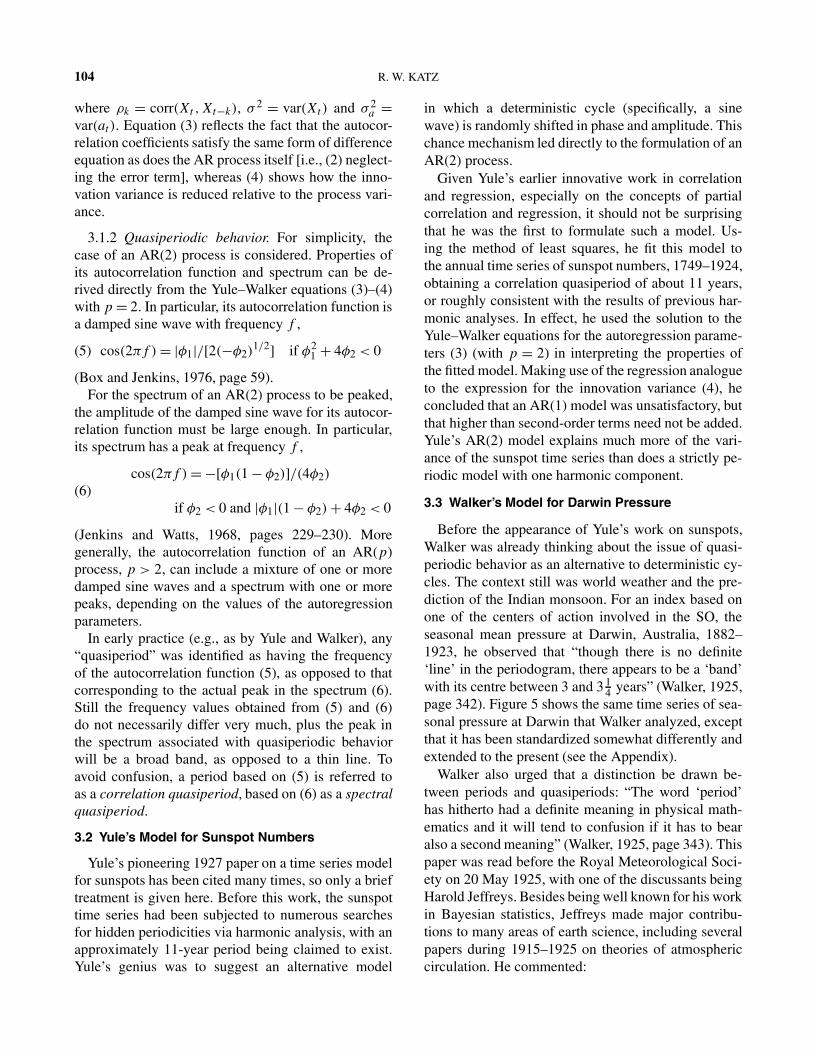
3.1.2 Quasiperiodic behavior. For simplicity, thecase of an AR(2) process is considered. Properties ofits autocorrelation function and spectrum can be de-rived directly from the Yule–Walker equations (3)–(4)with p = 2. In particular, its autocorrelation function isa damped sine wave with frequency f ,

cos(2πf ) = |φ1|/[2(−φ2)1/2] if φ2

1 + 4φ2 < 0(5)

(Box and Jenkins, 1976, page 59).For the spectrum of an AR(2) process to be peaked,

the amplitude of the damped sine wave for its autocor-relation function must be large enough. In particular,its spectrum has a peak at frequency f ,

cos(2πf ) = −[φ1(1 − φ2)]/(4φ2)

(6)if φ2 < 0 and |φ1|(1 − φ2) + 4φ2 < 0

(Jenkins and Watts, 1968, pages 229–230). Moregenerally, the autocorrelation function of an AR(p)process, p > 2, can include a mixture of one or moredamped sine waves and a spectrum with one or morepeaks, depending on the values of the autoregressionparameters.

In early practice (e.g., as by Yule and Walker), any“quasiperiod” was identified as having the frequencyof the autocorrelation function (5), as opposed to thatcorresponding to the actual peak in the spectrum (6).Still the frequency values obtained from (5) and (6)do not necessarily differ very much, plus the peak inthe spectrum associated with quasiperiodic behaviorwill be a broad band, as opposed to a thin line. Toavoid confusion, a period based on (5) is referred toas a correlation quasiperiod, based on (6) as a spectralquasiperiod.

3.2 Yule’s Model for Sunspot Numbers

Yule’s pioneering 1927 paper on a time series modelfor sunspots has been cited many times, so only a brieftreatment is given here. Before this work, the sunspottime series had been subjected to numerous searchesfor hidden periodicities via harmonic analysis, with anapproximately 11-year period being claimed to exist.Yule’s genius was to suggest an alternative model

in which a deterministic cycle (specifically, a sinewave) is randomly shifted in phase and amplitude. Thischance mechanism led directly to the formulation of anAR(2) process.

Given Yule’s earlier innovative work in correlationand regression, especially on the concepts of partialcorrelation and regression, it should not be surprisingthat he was the first to formulate such a model. Us-ing the method of least squares, he fit this model tothe annual time series of sunspot numbers, 1749–1924,obtaining a correlation quasiperiod of about 11 years,or roughly consistent with the results of previous har-monic analyses. In effect, he used the solution to theYule–Walker equations for the autoregression parame-ters (3) (with p = 2) in interpreting the properties ofthe fitted model. Making use of the regression analogueto the expression for the innovation variance (4), heconcluded that an AR(1) model was unsatisfactory, butthat higher than second-order terms need not be added.Yule’s AR(2) model explains much more of the vari-ance of the sunspot time series than does a strictly pe-riodic model with one harmonic component.

3.3 Walker’s Model for Darwin Pressure

Before the appearance of Yule’s work on sunspots,Walker was already thinking about the issue of quasi-periodic behavior as an alternative to deterministic cy-cles. The context still was world weather and the pre-diction of the Indian monsoon. For an index based onone of the centers of action involved in the SO, theseasonal mean pressure at Darwin, Australia, 1882–1923, he observed that “though there is no definite‘line’ in the periodogram, there appears to be a ‘band’with its centre between 3 and 3 1

4 years” (Walker, 1925,page 342). Figure 5 shows the same time series of sea-sonal pressure at Darwin that Walker analyzed, exceptthat it has been standardized somewhat differently andextended to the present (see the Appendix).

Walker also urged that a distinction be drawn be-tween periods and quasiperiods: “The word ‘period’has hitherto had a definite meaning in physical math-ematics and it will tend to confusion if it has to bearalso a second meaning” (Walker, 1925, page 343). Thispaper was read before the Royal Meteorological Soci-ety on 20 May 1925, with one of the discussants beingHarold Jeffreys. Besides being well known for his workin Bayesian statistics, Jeffreys made major contribu-tions to many areas of earth science, including severalpapers during 1915–1925 on theories of atmosphericcirculation. He commented:

CONNECTION BETWEEN EL NIÑO AND STATISTICS 105

with reference to the possibility of a realperiodicity of variable period, that such aphenomenon could be discovered, if it werepresent, by Clayton’s method in which cor-relation coefficients were worked out be-tween the value of the data and its val-ues one, two, three, etc., days afterwards(Walker, 1925, page 346).

Thus as early as 1925, Walker was given advice onhow he might formally model quasiperiodic behavior.

A subsequent paper, read before the Royal Meteo-rological Society by Walker on 18 November 1925,focuses on uses and abuses of correlation coefficients(Walker and Bliss, 1926). The British statistician Regi-nald Hooker, known for his ideas about detrending timeseries (Klein, 1997, Chapter 3), was one of the discus-sants and commented:

He had listened on the previous day toan extraordinarily interesting address at theStatistical Society by Mr. Udny Yule, whotook as his subject much the same prob-lem as Sir Gilbert Walker had taken, and hehoped that he and Sir Gilbert Walker mightcollaborate in the investigation of this sub-ject (Walker and Bliss, 1926, page 81).

The paper to which Hooker was referring had theprovocative title of “Why do we sometimes get non-sense-correlations between time-series?” (Yule, 1926),in some respects a precursor to Yule (1927). Evidently,no such collaboration between Yule and Walker evertook place. Yule’s 1927 paper turned out to be his

last significant research, because he retired in 1930and was a semiinvalid from 1931 onward (Kendall,1952). Nevertheless, Hooker was certainly prescientwith respect to the appearance of the term Yule–Walkerequations.

3.3.1 Derivation of Yule–Walker equations. As soonwill be explained, Walker’s application to Darwin pres-sure required a more complex model than an AR(2)process. So he was compelled to extend Yule’s ap-proach, considering an AR process of arbitrary order p

and deriving the general form of Yule–Walker equa-tions, (3)–(4) (Walker, 1931). Because the autocorrela-tion coefficients satisfy a relationship (3) identical tothat for the original process (2), Walker argued thatthe autocorrelation function “may be used to read offthe character of the natural periods” of the process(Walker, 1931, page 532). Wold (1938, pages 143–144)claims that Walker derived (3) only for lags k > p,but Walker actually stated that (3) holds “in general”(Walker, 1931, page 519) without specifying any con-ditions on k, so this issue is not completely clear.

3.3.2 Analysis of Darwin pressure. In the samepaper, Walker applied the general autoregressive modelto the seasonal time series of Darwin pressure, nowextended through winter 1926 (see Figure 5). Hismotivation was that Darwin is

one of the most important centres of ac-tion of “world weather,” which . . . displayssurges of varying amplitude and period withirregularities superposed, suggesting thatpressure in this region has a natural period

FIG. 5. Standardized time series of seasonal mean sea level pressure at Darwin, Australia, for winter 1882–fall 1998.

106 R. W. KATZ

of its own, based presumably on the physi-cal relationships of world-weather, but thatthe oscillations are modified by external dis-turbances (Walker, 1931, page 525).

Unlike the sunspot time series, the sample autocorre-lation function for the Darwin time series appeared tohim to have a more complex form than that of a dampedsine wave. For this reason, he considered a higher-order AR(p) process as a candidate model, observingthat the Yule–Walker equations (3) imply that the au-tocorrelation function is, in general, a sum of dampedexponential and damped sine waves (see Section 3.1).

However, Walker did not adopt Yule’s estimationmethod of fitting an AR process directly to the databy regression. Being preoccupied with the issue ofquasiperiodicity, he fit a mixture of one damped sinewave and two damped exponentials to the sampleautocorrelation function by trial and error. Next thisfitted autocorrelation function was converted into thecorresponding difference equation, which assumes theform of an AR(4) model. Still, he was cautious aboutdrawing any firm conclusions on the basis of the fittedAR(4) model alone: “There appears to be a periodicityof about 11 1

2 quarters . . . but the evidence that it isdamped is not conclusive” (Walker, 1931, page 531).

It turns out that this rather indirect approach to modelfitting does not necessarily result in sensible parame-ter estimates. Although Walker’s fitted model for theautocorrelation function matches reasonably well thefirst three or four sample autocorrelation coefficients,his indirectly derived AR(4) model does not. As laterpointed out by Wold (1938, pages 145–146), the dif-ficulty is that Walker’s fitted autocorrelation functiondoes not actually correspond to an AR process. Beforereturning to Wold’s assessment of Walker’s applicationin Section 4.1, it will be useful to reanalyze the Darwinpressure time series.

3.3.3 Reanalysis of Darwin pressure. The time se-ries of mean seasonal pressure at Darwin analyzed byWalker ranges from winter 1882 to winter 1926 (i.e.,a length of 177 seasons), or nearly the same num-ber of observations as the sunspot data as analyzedby Yule (Walker, 1931). To eliminate the annual cyclein mean pressure, Walker converted the data into de-viations from the corresponding seasonal mean. HereWalker’s analysis is repeated, with a few minor modi-fications that include making use of data corrected forinstrumental bias and removing the annual cycle in thepressure standard deviation. The Appendix gives moredetails on these changes, the rationale being that their

FIG. 6. Sample autocorrelation function of Darwin pressure,winter 1882–winter 1926.

nature is such that Walker would have been readily ableto implement them.

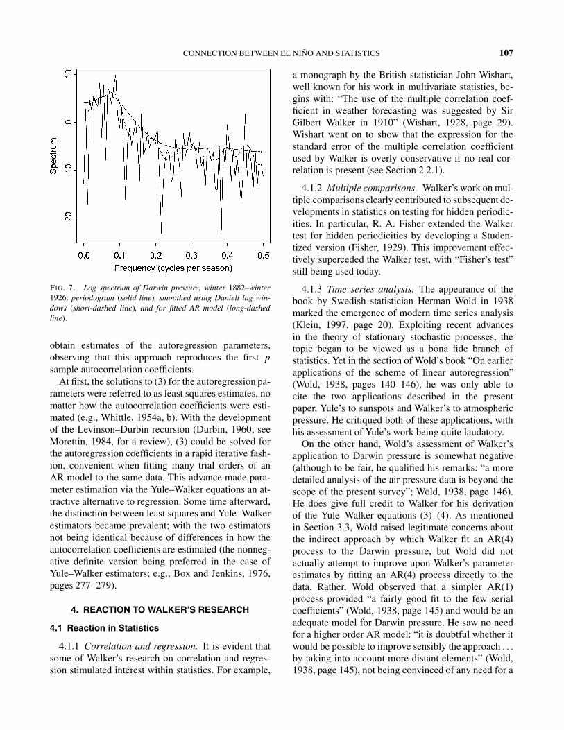
The reanalyzed data appear as the first portion of thetime series in Figure 5, except for slight differencesintroduced by the standardization being based ona shorter time period. The sample autocorrelationfunction (Figure 6) indicates at least weak evidenceof a damped oscillation. Walker obtained a similarpattern except for a tendency for the autocorrelationto remain positive at higher lags, apparently due to anartificial trend in the data introduced by instrumentalbias (see the Appendix). Figure 7 gives the rawperiodogram, a nonparametric smoothed spectrum andthe spectrum for an AR(4) model fitted by the Yule–Walker equations (3)–(4). A broad band is evident atabout 3 to 3 1

2 yr (i.e., at about 0.07 to 0.08 cycles perseason in Figure 7), but it is rather weak. Rather thandetermine the statistical significance of these estimatesdirectly, their reality will be examined in Section 5 inthe light of more recent observational evidence andtheoretical developments.

3.4 Etymology

The eponym Yule–Walker equations (or “relations”)did not originate until long after the work of Yule andWalker was published, with the earliest appearanceI have found being in Kendall (1949). Wold (1938,page 178) recognized the equivalence of the Yule–Walker equations to the normal equations that arisein least squares. He solved (3), for 1 ≤ k ≤ p, to

CONNECTION BETWEEN EL NIÑO AND STATISTICS 107

FIG. 7. Log spectrum of Darwin pressure, winter 1882–winter1926: periodogram (solid line), smoothed using Daniell lag win-dows (short-dashed line), and for fitted AR model (long-dashedline).

obtain estimates of the autoregression parameters,observing that this approach reproduces the first p

sample autocorrelation coefficients.At first, the solutions to (3) for the autoregression pa-

rameters were referred to as least squares estimates, nomatter how the autocorrelation coefficients were esti-mated (e.g., Whittle, 1954a, b). With the developmentof the Levinson–Durbin recursion (Durbin, 1960; seeMorettin, 1984, for a review), (3) could be solved forthe autoregression coefficients in a rapid iterative fash-ion, convenient when fitting many trial orders of anAR model to the same data. This advance made para-meter estimation via the Yule–Walker equations an at-tractive alternative to regression. Some time afterward,the distinction between least squares and Yule–Walkerestimators became prevalent; with the two estimatorsnot being identical because of differences in how theautocorrelation coefficients are estimated (the nonneg-ative definite version being preferred in the case ofYule–Walker estimators; e.g., Box and Jenkins, 1976,pages 277–279).

4. REACTION TO WALKER’S RESEARCH

4.1 Reaction in Statistics

4.1.1 Correlation and regression. It is evident thatsome of Walker’s research on correlation and regres-sion stimulated interest within statistics. For example,

a monograph by the British statistician John Wishart,well known for his work in multivariate statistics, be-gins with: “The use of the multiple correlation coef-ficient in weather forecasting was suggested by SirGilbert Walker in 1910” (Wishart, 1928, page 29).Wishart went on to show that the expression for thestandard error of the multiple correlation coefficientused by Walker is overly conservative if no real cor-relation is present (see Section 2.2.1).

4.1.2 Multiple comparisons. Walker’s work on mul-tiple comparisons clearly contributed to subsequent de-velopments in statistics on testing for hidden periodic-ities. In particular, R. A. Fisher extended the Walkertest for hidden periodicities by developing a Studen-tized version (Fisher, 1929). This improvement effec-tively superceded the Walker test, with “Fisher’s test”still being used today.

4.1.3 Time series analysis. The appearance of thebook by Swedish statistician Herman Wold in 1938marked the emergence of modern time series analysis(Klein, 1997, page 20). Exploiting recent advancesin the theory of stationary stochastic processes, thetopic began to be viewed as a bona fide branch ofstatistics. Yet in the section of Wold’s book “On earlierapplications of the scheme of linear autoregression”(Wold, 1938, pages 140–146), he was only able tocite the two applications described in the presentpaper, Yule’s to sunspots and Walker’s to atmosphericpressure. He critiqued both of these applications, withhis assessment of Yule’s work being quite laudatory.

On the other hand, Wold’s assessment of Walker’sapplication to Darwin pressure is somewhat negative(although to be fair, he qualified his remarks: “a moredetailed analysis of the air pressure data is beyond thescope of the present survey”; Wold, 1938, page 146).He does give full credit to Walker for his derivationof the Yule–Walker equations (3)–(4). As mentionedin Section 3.3, Wold raised legitimate concerns aboutthe indirect approach by which Walker fit an AR(4)process to the Darwin pressure, but Wold did notactually attempt to improve upon Walker’s parameterestimates by fitting an AR(4) process directly to thedata. Rather, Wold observed that a simpler AR(1)process provided “a fairly good fit to the few serialcoefficients” (Wold, 1938, page 145) and would be anadequate model for Darwin pressure. He saw no needfor a higher order AR model: “it is doubtful whether itwould be possible to improve sensibly the approach . . .by taking into account more distant elements” (Wold,1938, page 145), not being convinced of any need for a

108 R. W. KATZ

model with quasiperiodic behavior: “this periodogramdoes not like that of the sunspots suggest a scheme oflinear autoregression with a tendency to periodicity”(Wold, 1938, page 146).

4.2 Reaction in Meteorology

4.2.1 General. During the time span of Walker’s re-search career, the general reaction within the meteo-rological community to statistical methods, especiallycorrelation and regression, was extreme skepticism.For example, a rather technical paper, making exten-sive use of correlation in modeling rainfall, was readby Fisher before the Royal Meteorological Society on19 April 1922 (Fisher and Mackenzie, 1922). In thediscussion of this paper, it was mentioned that “no newmeteorological fact had been discovered by means ofcorrelation coefficients; certainly up to the present nopractical forecasts had been obtained from correlationcoefficients” (Fisher and Mackenzie, 1922, page 242).

So it should not be surprising that Walker’s researchdiscoveries were met with much resistance withinmeteorology. For example, concerning his pioneeringuse of correlation in meteorology, Normand (1953,page 464) noted that “meteorologists have not allaccorded him whole-hearted thanks.”

4.2.2 Forecasting. Because the potential value oflong-range weather forecasts was perceived to be high,Walker’s research did draw much attention, but doubtsremained about reliance on statistical methods. Forinstance, in a review of the series of memoirs ofthe Indian Meteorological Department produced byWalker, the British meteorologist William Dines (1916,page 130) argued that “correlation is of very little usefor the purpose of forecasting unless the coefficientsconcerned are very high.” Dines did admit that “forthe purpose of investigating relationships betweenvarious elements and their physical causes correlationcoefficients, and more especially partial ones, are ofvery great importance.” Walker’s response to Dineswas to observe that “the object of weather forecastingbeing practical, we cannot wait until we are absolutelycertain of our results” (Walker, 1918, page 223).

Over the years, there were several attempts to “ver-ify” Walker’s correlations and multiple regressionequations for seasonal forecasting, generally by re-calculating the same statistics as the number of ob-servations increased (e.g., Montgomery, 1937). Grant(1956, page 10) questioned Walker’s multiple regres-sion equations for predicting rainfall in India, conclud-ing that: “the observed correlations do not prove or

even render likely the existence of correlations of use-ful magnitude between past and future weather.” Inseveral instances, the correlations appear to weakenwith more data, but not necessarily greater changesthan could be reasonably attributable to sampling vari-ations (e.g., Gershunov, Schneider and Barnett, 2001).

4.2.3 Physical explanation. Despite his reliance onstatistics, Walker always sought physical explanations:“The number of satisfactorily established relationshipsbetween weather in different parts of the world issteadily growing . . . and I cannot help believing thatwe shall gradually find out the physical mechanism bywhich these are maintained” (Walker, 1918, page 223).Despite his lack of formal training in meteorology, hetried to lay out possible research avenues. In an addressto the Royal Meteorological Society, he suggested that“variations in activity of the general oceanic circula-tion will be much more far reaching and important”(Walker, 1927a, page 113) in explaining pressure os-cillations such as the SO, and he later recommendedsearching “for an explanation in terms of slowly chang-ing features, such as ocean temperatures” (Walker,1936b, page 136).

For reasons that are not completely clear, Walker’sappeals for physical explanations went largely un-heeded. At the time of his death in 1958, his work wascharacterized in terms of unrealized expectations:

Walker’s hope was presumably not onlyto unearth relations useful for forecastingbut to discover sufficient and sufficientlyimportant relations to provide a productivestarting point for a theory of world weather.It hardly appears to be working out like that(Sheppard, 1959, page 186).

With the recent popularity of the ENSO phenom-enon, it is difficult to appreciate that: “As recentlyas the 1960s, the SO was still largely dismissed as aclimate curiosity” (Rasmusson, 1991, page 310). Theconventional explanation in meteorology is that onlywith the breakthrough by Bjerknes (1969) (see the In-troduction and Section 2.2.1) was the physical theoryavailable to take advantage of Walker’s work. Surely,more rapid progress would have been achieved if re-searchers in meteorology had taken seriously Walker’sdiscoveries, rather than tending to dismiss them (foradditional discussion of the reaction to Walker’s workwithin meteorology, see Brown and Katz, 1991).

CONNECTION BETWEEN EL NIÑO AND STATISTICS 109

5. PRESENT STATE OF MODELING THESOUTHERN OSCILLATION

Not only has the sunspot time series that Yule mod-eled become one of the most analyzed data sets instatistics, but on occasion it still is used in meteorol-ogy as well to search for sun–weather connections. Onthe other hand, the SO time series, originally modeledby Walker, received very little attention within mete-orology until recent decades. It is therefore somewhatironic that, at least for long-range weather or climateforecasting, sunspots have proved of so little value(e.g., Pittock, 1978), whereas today the ENSO phe-nomenon is the primary focus of attention. At least inthis respect, it appears that Walker’s research discover-ies have stood the test of time well.

Since Walker’s era, the observational informationabout the SO has improved. Longer and more reliablerecords exist as well as refined indices, such as thedifference between Tahiti and Darwin pressure (seeFigure 4), designed to reflect explicitly the two centersof action involved in the SO pressure seesaw (Walkerdid not make use of Tahiti pressure measurements, andsome doubts have been raised about their reliabilitybefore 1935; e.g., Trenberth and Hoar, 1996). Progressalso has been made on the dynamical underpinnings ofthe more general ENSO phenomenon.

5.1 Quasiperiodic Behavior

Recalling the discussion in Section 3.3 about the SObeing a quasiperiodic phenomenon (see Figure 7), littledoubt remains about this issue within the meteorologycommunity. For example, Chu and Katz (1989) used anAR(3) process for the seasonal Tahiti–Darwin pressuredifference since 1935, obtaining an estimated spectralquasiperiod of about 3.6 years; and Trenberth andHoar (1996) modeled the seasonal Darwin time seriesfor 100 years from 1882 to 1981 (i.e., much of thesame data shown in Figure 5) with an ARMA(3, 1)process yielding an estimated spectral quasiperiod ofabout 4.2 years. The SO time series even has appearedrecently in the statistics literature, with Huerta andWest (1999) performing a fully Bayesian analysis(involving the use of Markov chain Monte Carlomethods) of the Tahiti–Darwin pressure differenceaggregated to a monthly time scale starting in 1950.Their posterior distribution on the order p of an ARprocess attaches nonnegligible probability between 8and 17 [roughly consistent with the findings of Chu andKatz (1989), who selected an ARMA(7, 1) model formonthly data over a slightly different time period], and

they obtained an estimated spectral quasiperiod of 4 to5 years (Chu and Katz, 3.3 years). So, notwithstandingthe limitations in Walkers’s original analysis of theDarwin data, his insight about the SO phenomenonappears to be essentially correct.

5.2 Nonlinear Dynamics

The quasiperiodic feature of the ENSO phenomenonnow is viewed as fundamental (Graham and White,1988), but with its source remaining unclear (e.g.,Wang, 2001). The prevailing dynamical explanation isthe “delayed oscillator hypothesis” originally formu-lated by Suarez and Schopf (1988), with alternativeversions subsequently being proposed (Wang, 2001).All of these conceptual models involve deterministicnonlinear equations, making use of both positive andnegative feedbacks between the atmosphere and oceanin the equatorial Pacific to produce an oscillation onthe interannual time scale of ENSO. To obtain the qua-siperiodic behavior of the actual ENSO phenomenon,a stochastic forcing term sometimes has been added tothe model (Graham and White, 1988). In a sense, thisapproach is reminiscent of Yule’s original idea of intro-ducing randomness into a strictly periodic oscillation.

Finally, it should be noted that general circulationmodels (GCM’s), very complex deterministic numeri-cal models of the atmosphere–ocean system, likewiseare starting to be capable of generating “ENSO-like”behavior. For example, Meehl and Arblaster (1998)found that one particular GCM, the NCAR ClimateSystem Model, produces a spectral quasiperiod ofabout 4 yr or quite close to that observed for ENSO.For reasons that are not yet understood, many GCM’sexhibit a peak at shorter periods than that observed(AchutaRao et al., 2000).

6. DISCUSSION

Sir Gilbert Walker’s contribution to the Yule–Walkerequations arose in conjunction with an attempt to de-velop a quasiperiodic model for the Southern Oscil-lation, a pressure seesaw closely related to the ElNiño phenomenon. The question remains of why hashis work concerning the SO, other pressure oscilla-tions and related teleconnections proved so success-ful. Within meteorology, the somewhat parochial ex-planation is that it must have been Walker’s climato-logical expertise. In my judgment, however, it was hisexpertise in mathematics and statistics, coupled witha dedicated effort to solve a particular scientific prob-lem (namely, long-range weather or climate forecast-ing) that best explains this success.

110 R. W. KATZ

A heightened level of interest in collaborative re-search between statistics and the environmental sci-ences and geosciences now exists (e.g., Chelton, 1994;Nychka, 2000; Piegorsch, Smith, Edwards and Smith,1998). However, the lessons gleaned from the earlierhistory of collaboration in such areas ought to be appre-ciated as well. In this vein, one last quote from Walkeris germane:

There is, to-day, always a risk that spe-cialists in two subjects, using languagesfull of words that are unintelligible withoutstudy, will grow up not only, without knowl-edge of each other’s work, but also willignore the problems which require mutualassistance.—Sir Gilbert T. Walker (Walker,1927b, page 321)

APPENDIX

The time series of monthly mean Darwin pressure,for the period January 1882–present, is available froma Web site maintained by the Climate Prediction Cen-ter of the National Oceanic and Atmospheric Admin-istration (NOAA): http://www.cpc.ncep.noaa.gov/data/indices/index.html. The seasonal time series, originallyanalyzed by Walker (1931), was reconstructed fromthis NOAA data set. Because it is not possible tospecify the initial state of the time series (i.e., winter1882), the required value for December 1881 was ob-tained from another source, a Web site maintained bythe Australian Bureau of Meteorology Research Cen-tre: ftp://ftp.bom.gov.au/anon/home/ncc/www/sco/soi/darwinmslp.html.

Since the time Walker analyzed this data, a correc-tion has been applied to remove an artificial trend in-troduced by instrumental drift. This trend actually wasnoticed by Walker (1931, page 529), and he suspecteda source such as “some change of barometric correc-tion.” Yet he did not remove this trend and argued that“its effect on periodicity will be insignificant.” Inci-dentally, Walker was a contributor to the collection inwhich these corrected pressures were published (Clay-ton, 1934, page 575). In fact, the impetus for this se-ries of publications of weather records was research onworld weather in which Walker was one of the initia-tors.

In constructing atmospheric or oceanic circulationindices, today it is common to adjust for annual cy-cles in the mean and standard deviation simply by stan-dardizing each month or season separately (i.e., sub-tracting the corresponding sample mean and then di-viding by the sample standard deviation) (e.g., Tren-berth and Hoar, 1996). Although Walker only removed

the seasonal mean in his analysis of Darwin pressure,he did make much use of standardized variables inother work. In particular, he usually expressed multi-ple regression equations in this form, both for compu-tational convenience and for ease in interpretation (e.g.,Walker, 1910). In addition, his correlation or regressionanalyses generally were conducted separately for eachseason (i.e., stratifying the data by the season to be pre-dicted), because he was aware of the possibility thatvariability and covariability might differ depending onthe time of year (e.g., Walker, 1924).

ACKNOWLEDGMENTS

The inspiration for this work originated in a collab-oration with Barbara Brown. I thank Rolando Garcia,Judy Klein, Gene Rasmusson, Malcolm Walker, PeterWhittle and especially Rob Allan for advice and com-ments. I also gratefully acknowledge one of the Edi-tors, whose suggestions helped improve the presenta-tion. Research was supported in part by NSF GrantsDMS-93-12686 and DMS-98-15344 to the NationalCenter for Atmospheric Research’s Geophysical Sta-tistics Project; NCAR is sponsored by the National Sci-ence Foundation.

REFERENCES

ACHUTARAO, K., SPERBER, K. R. and 13 OTHERS (2000). ElNiño Southern Oscillation in coupled GCMs. PCMDI Report61, Program for Climate Model Diagnosis and Intercompari-son, Lawrence Livermore National Laboratory, Univ. Califor-nia.

ALLAN, R., LINDESAY, J. and PARKER, D. (1996). El Niño South-ern Oscillation and Climate Variability. CSIRO Publishing,Melbourne.

ANDERSON, T. W. (1971). The Statistical Analysis of Time Series.Wiley, New York.

BJERKNES, J. (1969). Atmospheric teleconnections from theequatorial Pacific. Monthly Weather Review 97 163–172.

BOX, G. E. P. and JENKINS, G. M. (1976). Time Series Analysis:Forecasting and Control, rev. ed. Holden-Day, San Francisco.

BRAUN, H. I., ed. (1994). The Collected Works of John W.Tukey, V. VIII, Multiple Comparisons: 1948–1983. Wadsworth,Belmont, CA.

BROWN, B. G. and KATZ, R. W. (1991). Use of statistical methodsin the search for teleconnections: past, present, and future.In Teleconnections Linking Worldwide Climate Anomalies:Scientific Basis and Societal Impact (M. H. Glantz, R. W. Katzand N. Nicholls, eds.) 371–400. Cambridge Univ. Press.

CAVE-BROWNE-CAVE, F. E. (1904). On the influence of the timefactor in the correlation between the barometric heights atstations more than 1,000 miles apart. Proc. Roy. Soc. LondonSer. A 74 403–413.

CHANGNON, S. A., ed. (2000). El Niño, 1997–1998: The ClimateEvent of the Century. Oxford Univ. Press.

CONNECTION BETWEEN EL NIÑO AND STATISTICS 111

CHAPMAN, S. (1934). Symons Memorial Medal, 1934. QuarterlyJournal of the Royal Meteorological Society 60 184–185.

CHELTON, D. B. (1994). Physical oceanography: a brief overviewfor statisticians. Statist. Sci. 9 150–166.

CHU, P.-S. and KATZ, R. W. (1989). Spectral estimation fromtime series models with relevance to the Southern Oscillation.Journal of Climate 2 86–90.

CLAYTON, H. H. (1917). Effect of short period variations of so-lar radiation on the Earth’s atmosphere. Smithsonian Miscella-neous Collections 68 1–18.

CLAYTON, H. H., ed. (1934). World weather records. Part IV.(Errata in Volume 79.) Smithsonian Miscellaneous Collections90 573–589.

CRUTZEN, P. J. and RAMANATHAN, V. (2000). The ascent ofatmospheric sciences. Science 290 299–304.

DAVIS, H. T. (1941). The Analysis of Economic Time Series.Principia Press, Bloomington, IN.

DAVIS, M. (2001). Late Victorian Holocausts: El Niño Faminesand the Making of the Third World. Verso, London.

DIAZ, H. F. and MARKGRAF, V., eds. (1992). El Niño: Historicaland Paleoclimatic Aspects of the Southern Oscillation. Cam-bridge Univ. Press.

DIAZ, H. F. and MARKGRAF, V., eds. (2000). El Niño and theSouthern Oscillation: Multiscale Variability and Global andRegional Impacts. Cambridge Univ. Press.

DINES, W. H. (1916). Review of “Correlation in seasonal varia-tions of weather, I–VI.” Memoirs of the Indian MeteorologicalDepartment by G. T. Walker. Quarterly Journal of the RoyalMeteorological Society 42 129–132.

DURBIN, J. (1960). The fitting of time-series models. Internat.Statist. Rev. 28 233–244.

FISHER, R. A. (1929). Tests of significance in harmonic analysis.Proc. Roy. Soc. London Ser. A 125 54–59.

FISHER, R. A. and MACKENZIE, W. A. (1922). The correlationof weekly rainfall (with discussion). Quarterly Journal of theRoyal Meteorological Society 48 234–245.

GERSHUNOV, A., SCHNEIDER, N. and BARNETT, T. (2001).Low-frequency modulation of the ENSO–Indian monsoonrainfall relationship: signal or noise? Journal of Climate 142486–2492.

GLANTZ, M. H. (2001). Currents of Change: Impacts of El Niñoand La Niña on Climate and Society, 2nd ed. Cambridge Univ.Press.

GLANTZ, M. H., KATZ, R. W. and NICHOLLS, N., eds. (1991).Teleconnections Linking Worldwide Climate Anomalies: Sci-entific Basis and Societal Impact. Cambridge Univ. Press.

GRAHAM, N. E. and WHITE, W. B. (1988). The El Niño cycle:a natural oscillator of the Pacific ocean–atmosphere system.Science 240 1293–1302.

GRANT, A. M. (1956). The application of correlation and regres-sion to forecasting. Meteorological Study 7, Bureau of Meteo-rology, Melbourne, Australia.

HUERTA, G. and WEST, M. (1999). Priors and component struc-tures in autoregressive time series models. J. Roy. Statist. Soc.Ser. B 61 881–899.

HURRELL, J. W. (1995). Decadal trends in the North AtlanticOscillation: regional temperatures and precipitation. Science269 676–679.

HURRELL, J. W. (1996). Influence of variations in extratropicalwintertime teleconnections on Northern Hemisphere tempera-ture. Geophys. Res. Lett. 23 665–668.

JENKINS, G. M. and WATTS, D. G. (1968). Spectral Analysis andIts Applications. Holden-Day, San Francisco.

KATZ, R. W. and BROWN, B. G. (1991). The problem of multi-plicity in research on teleconnections. International Journal ofClimatology 11 505–513.

KENDALL, M. G. (1945). On the analysis of oscillatory time-series(with discussion). J. Roy. Statist. Soc. 108 93–141.

KENDALL, M. G. (1949). The estimators of parameters in linearautoregressive time series. Econometrica 17 (supplement) 44–57.

KENDALL, M. G. (1952). George Udny Yule, C.B.E., F.R.S.J. Roy. Statist. Soc. Ser. A 115 156–161.

KLEIN, J. L. (1997). Statistical Visions in Time: A History of TimeSeries Analysis, 1662–1938. Cambridge Univ. Press.

LAMB, P. J. and PEPPLER, R. A. (1987). North Atlantic Oscil-lation: concept and an application. Bulletin of the AmericanMeteorological Society 68 1218–1225.

LOCKYER, N. and LOCKYER, W. J. S. (1904). The behavior of theshort-period atmospheric pressure variation over the Earth’ssurface. Proc. Roy. Soc. London 73 457–470.

MEEHL, G. A. and ARBLASTER, J. M. (1998). The Asian–Australian monsoon and El Niño–Southern Oscillation in theNCAR Climate System Model. Journal of Climate 11 1356–1385.

MONTGOMERY, R. B. (1937). Verification of three of Walker’sseasonal forecasting formulae for India monsoon rain. Bulletinof the American Meteorological Society 18 287–290.

MORETTIN, P. A. (1984). The Levinson algorithm and its applica-tions in time series analysis. Internat. Statist. Rev. 52 83–92.

NORMAND, C. (1953). Monsoon seasonal forecasting. QuarterlyJournal of the Royal Meteorological Society 79 463–473.

NORMAND, C. (1958). Sir Gilbert Walker, C.S.I., F.R.S. Nature182 1706.

NYCHKA, D. (2000). Challenges in understanding the atmosphere.J. Amer. Statist. Assoc. 95 972–975.

PHILANDER, S. G. (1990). El Niño, La Niña, and the SouthernOscillation. Academic Press, San Diego.

PIEGORSCH, W. W., SMITH, E. P., EDWARDS, D. and SMITH,R. L. (1998). Statistical advances in environmental science.Statist. Sci. 13 186–208.

PITTOCK, A. B. (1978). Critical look at long-term sun–weatherrelationships. Reviews of Geophysics and Space Physics 16400–420.

RASMUSSON, E. M. (1991). Observational aspects of ENSO cycleteleconnections. In Teleconnections Linking Worldwide Cli-mate Anomalies: Scientific Basis and Societal Impact (M. H.Glantz, R. W. Katz and N. Nicholls, eds.) 309–343. CambridgeUniv. Press.

SCHUSTER, A. (1898). On the investigation of hidden periodicitieswith application to a supposed 26-day period of meteorologicalphenomena. Terrestrial Magnetism 3 13–41.

SHEPPARD, P. A. (1959). Sir Gilbert Walker, C.S.I., F.R.S.Quarterly Journal of the Royal Meteorological Society 85 186.

SIMPSON, G. C. (1959). Sir Gilbert T. Walker, C.S.I., F.R.S.Weather 14 67–68.

SUAREZ, M. J. and SCHOPF, P. S. (1988). A delayed actionoscillator for ENSO. J. Atmospheric Sci. 45 3283–3287.

112 R. W. KATZ

TAYLOR, G. I. (1962). Gilbert Thomas Walker, 1868–1958.Biographical Memoirs of Fellows of the Royal Society 8 166–174.

TRENBERTH, K. E. (1991). General characteristics of El Niño–Southern Oscillation. In Teleconnections Linking WorldwideClimate Anomalies: Scientific Basis and Societal Impact(M. H. Glantz, R. W. Katz and N. Nicholls, eds.) 13–42. Cam-bridge Univ. Press.

TRENBERTH, K. E. and CARON, J. M. (2000). The SouthernOscillation revisited: sea level pressures, surface temperatures,and precipitation. Journal of Climate 13 4358–4365.

TRENBERTH, K. E. and HOAR, T. J. (1996). The 1990–1995 ElNiño–Southern Oscillation event: longest on record. Geophys.Res. Lett. 23 57–60.

WALKER, G. T. (1910). Correlation in seasonal variations ofweather. II. Memoirs of the Indian Meteorological Department21(Part 2) 22–45.

WALKER, G. T. (1914). Correlation in seasonal variations ofweather. III. On the criterion for the reality of relationships orperiodicities. Memoirs of the Indian Meteorological Depart-ment 21(Part 9) 13–15.

WALKER, G. T. (1918). Correlation in seasonal variations ofweather. Quarterly Journal of the Royal Meteorological So-ciety 44 223–224.

WALKER, G. T. (1923). Correlation in seasonal variations ofweather. VIII. A preliminary study of world-weather. Memoirsof the Indian Meteorological Department 24(Part 4) 75–131.

WALKER, G. T. (1924). Correlation in seasonal variations ofweather. IX. A further study of world weather. Memoirs of theIndian Meteorological Department 24(Part 9) 275–332.

WALKER, G. T. (1925). On periodicity (with discussion). Quar-terly Journal of the Royal Meteorological Society 51 337–346.

WALKER, G. T. (1927a). The Atlantic Ocean. Quarterly Journalof the Royal Meteorological Society 53 97–113.

WALKER, G. T. (1927b). Review of “Climate through the Ages.A Study of Climatic Factors and Climatic Variations” byC. E. P. Brooks. Quarterly Journal of the Royal MeteorologicalSociety 53 321–323.

WALKER, G. T. (1930). On periodicity III—criteria for reality.Memoirs of the Royal Meteorological Society 3 97–101.

WALKER, G. T. (1931). On periodicity in series of related terms.Proc. Roy. Soc. London Ser. A 131 518–532.

WALKER, G. T. (1936a). Editorial. Quarterly Journal of the RoyalMeteorological Society 62 1–2.

WALKER, G. T. (1936b). Seasonal weather and its prediction.Smithsonian Institution Annual Report for 1935 117–138.

WALKER, G. T. and BLISS, E. W. (1926). On correlation coeffi-cients, their calculation use (with discussion). Quarterly Jour-nal of the Royal Meteorological Society 52 73–84.

WALKER, J. M. (1997). Pen portraits of presidents—Sir GilbertWalker, CSI, ScD, MA, FRS. Weather 52 217–220.

WALLACE, J. M. and GUTZLER, D. S. (1981). Teleconnections inthe geopotential height field during the Northern Hemispherewinter. Monthly Weather Review 109 784–812.

WANG, C. (2001). A unified oscillator model for the El Niño–Southern Oscillation. Journal of Climate 14 98–115.

WHITTLE, P. (1954a). The statistical analysis of a seiche record.Journal of Marine Research 13 76–100.

WHITTLE, P. (1954b). A statistical investigation of sunspot obser-vations with special reference to H. Alfvén’s sunspot model.Astrophysical Journal 120 251–260.

WHITTLE, P. (1963). Prediction and Regulation. Van Nostrand,Princeton.

WISHART, J. (1928). On errors in the multiple correlation coeffi-cient due to random sampling. Memoirs of the Royal Meteoro-logical Society 2 29–37.

WOLD, H. (1938). A Study in the Analysis of Stationary TimeSeries. Almqvist and Wiksell, Stockholm.

YULE, G. U. (1926). Why do we sometimes get nonsense-correlations between time-series?—A study in sampling andthe nature of time-series. J. Roy. Statist. Soc. 89 1–64.

YULE, G. U. (1927). On a method of investigating periodicitiesin disturbed series, with special reference to Wolfer’s sunspotnumbers. Philos. Trans. Roy. Soc. London Ser. A 226 267–298.