statistical process control with special …vuir.vu.edu.au/15709/1/tang_1996compressed.pdf ·...
TRANSCRIPT

STATISTICAL PROCESS CONTROL WITH
SPECIAL REFERENCE TO MULTIVARIABLE
PROCESSES AND SHORT RUNS
Pak Fai Tang
A thesis submitted in fialfilment of the requirements for
the degree of Doctor of Philosophy
Department of Computer and Mathematical Sciences
Faculty of Science
Victoria University of Technology
July, 1996

FTS THESIS 658.562015195 TAN 30001005084969 Tang, Pak Fai Statistical process control wi.M special reference to fnuJ^Tyaj^able processes and

CONTENTS
Chapter Page
Acknowledgments i
Declaration ii Abstract iii List of Figures vii List of Tables x
1. Introduction 1.1 Introduction to SPC 1 1.2 Problems of Traditional SPC for Short Production Runs 4 1.3 Multivariate Quality Control 6 1.4 Thesis Objectives 7
2. Literature Review 2.1 Introduction 9 2.2 Adjusting Control Limits Based on The Number of Subgroups or
Observations 9 2.3 Control Charts Based on Individual Measurements 12 2.4 Mixing Production Lots and Normalizing Output Data 15 2.5 Setup Variation and Measurement Error Considerations 19 2.6 'Self-Starting' Procedures Based on 'Running' Estimates of the
Process Parameters 21 2.7 Control Based on Exponentially Weighted Moving Averages
(EWMA) 29 2.8 Deriving'Control'Limits From Specifications 35 2.9 Adjusting Set-up Continuously Based on Process Output 37 2.10 Monitoring Process Input Parameters 39 2.11 Economically Optimal Control Procedures 40
3. Mean Control for Multivariate Normal Processes 3.1 Introduction 45 3.2 Methodological Basis 46 3.3 Monitoring the Mean of Multivariate Normal Processes 53
3.3.1 Control Charts Based on Individual Measurements 54 3.3.2 Control Charts Based on Subgroup Data 57
3.4 Example 63 3.5 Control Performance 79 3.6 Detecting Step Shifl:s and Linear Trends Using A Robust Estimator
of Z andEWMA 85 3.7 Computational Requirements 102
4. Dispersion Control for Multivariate Normal Processes 4.1 Introduction 109 4.2 Methodology I l l 4.3 Monitoring the Dispersion of Multivariable Processes 121

4.4 Rank-Deficient Problem 129 4.5 Comparisons 131 4.6 An Example 149 4.7 Effect of Aggregation on Control Performance 154
5. Capability Indices for Multivariate Processes 5.1 Introduction 158 5.2 A Review of Multivariate Capability Indices 160 5.3 Constructing a Multivariate Capability Index 166 5.4 Three Bivariate Capability Indices 168
5.4.1 Projection of Exact Ellipsoid Containing a Specified Proportion of Products 169
5.4.2 Bonferroni-Type Process Rectangular Region 171 5.4.3 Process Rectangular Region Based on Sidak's Probability
Inequality 172 5.5 Some Comparisons of The Projected, Bonferroni and Sidak-Type
Capability Indices 174 5.6 Testing The Capability of a Bivariate Process 176 5.7 Robustness to Departures From Normality - Some Consideration 180
6. A Comparison of Mean and Range Charts With The Method of Pre-Control 6.1 Introduction 185 6.2 A Review of Pre-Control 186 6.3 The Practical Merits of Pre-Control 190 6.4 Short Runs and Pre-Control 192 6.5 A Statistical Comparison Between Pre-Control and X-bar and R
Charts 193 6.6 Equating Sampling Effort 203 6.7 Concluding Remarks 208
7. Conclusions and Some Suggestions for Future Investigation 7.1 Summary and Conclusions 210 7.2 Suggestions for Future Work 213
References 215 Appendices 226 Simulation Programs 251

ACKNOWLEDGMENTS
I wish to express my sincere gratitude to my principal supervisor, Associate
Professor Neil Bamett and co-supervisor. Associate Professor Peter Cerone for helpfiil
suggestions, advice, guidance and encouragement throughout this project.
Special thanks are also due to Associate Professor Ian Murray and his wife
Glenice for their warm hospitality during my stay in AustraUa, Dr. Ng Lay Swee, the
principal of Tunku Abdul Rahman College, Malaysia for her advice and encouragement,
the Department of Computer and Mathematical Sciences, Victoria University of
Technology for the financial support given to me, and Tunku Abdul Rahman College for
the study leave period granted.
I am also indebted to the staff of the Department, particularly, Tom Peachey, Neil
Diamond, Alan Glasson, Ian Gomm, Ted Alwast, P.Rajendran (Raj) and Damon
Burgess, and my fellow colleagues, particularly, Mehmet Tat, Gregory Simmons,
Violetta Misiorek, Kevin Liu, Fred Liu, Rafyul Fatri, Phillip Tse and Simon So, who
have, in one way or another, rendered their kind assistance.
Finally, and most importantly, I would like to express my sincerest gratitude to
my wife, Susie and my father. Tang Yik Sang for their patience, continuous support and
encouragement. Without this, the project would not have been made possible.

DECLARATION
I hereby declare that:
(i) the following thesis contains only my original work which has not been
submitted previously, in whole or in part, in respect of any other academic
award, and
(ii) due acknowledgment has been made in the text of the thesis to all other material
used.
CpakFSr^g July, 1996
u

ABSTRACT
The quest for control and the subsequent pursuit of continuous quality
improvement in the manufacturing sector, due to mcreasingly keen competition, has
stimulated interest in statistical process control (SPC). Whilst traditional SPC techniques
are well suited to the mass production industries, their usefiilness in short run or low
volume manufacturing environments is questionable. The major problem with short-run
SPC is lack of data for estimation of the control parameters. In view of this limitation,
many alternatives and adaptations of existing techniques have been devised. However,
these efforts have largely been devoted to monitoring and controlling univariate
processes.
In practice, the quality of manufactured products is oflien determined by reference
to several quality characteristics which are correlated. Under these circumstances, it is
necessary to use multivariate quality control procedures which take the correlational
structure into consideration. Although this area has received considerable attention in the
literature, most of the published work assumes that prior information about the process
parameters is available. This assumption is rarely the case in the short run environment.
This thesis is primarily concerned with the development of multivariate quality
control procedures that can be effectively used in situations where prior estimates of the
process parameters are unavailable. For completeness, some better alternatives to
previously proposed procedures are also provided for the case where the process
parameters are assumed known in advance of production. These techniques are intended
for detecting a shift in the mean vector, the variance-covariance matrix and other process
disturbances. Using the proposed procedures, control can be initiated early in
ui

production, whether or or not prior information about the process parameters is
available.
The techniques presented for controlling the mean vector of multivariate
processes utiUze the probability integral transformation technique in order to produce
sequences of independent or approximately independent standard normal variables. This
offers greater flexibility than the 2-stage procedures recommended by some authors in
the design of control charts for the unknown parameter case. Apart fi-om the
conventional rule that signals when a plotted value exceeds either of the 3-sigma limits,
run tests as well as the methods of Cumulative Sum (CUSUM) and Exponentially
Weighted Moving Average (EWMA) can be used. A simulation study indicates that the
techniques, with the usual decision rule imposed, are particularly usefiil for 'picking up' a
persistent change in the process mean vector when subgroup data are used, even if prior
information about the process parameters is not available. For detecting step shifts and
linear trends based on individual observations, two specifically designed EWMA charts
based on similarly transformed variables but which use a different estimator of the
process variance-covariance matrix are found to be much more effective than other
competing procedures.
For dispersion control, use is made of the independent statistics that result from
the decomposition of variance-covariance matrices and the modified likelihood ratio
statistic for testing the equality of several covariance matrices, for the cases with known
and unknown dispersion parameters respectively. The proposed techniques are based on
some aggregate-type indices computed from such independent variables. It is found that
these techniques outperform previously proposed procedures for many sustained shifts in
the process variance-covariance matrix. In addition, it is demonstrated that the dispersion
IV

control chart, for the known parameters case, is more sensitive to certain shifts than that
which involves separate charting of the standardized variances of the principal
components or the individual variables resuhing from the partitioning of the variance-
covariance matrices. The proposed techniques also possess some practical advantages
over existing procedures. In particular, better control over the false signal rate, ease of
locating control limits and identification of the nature of process changes.
To satisfactorily describe the capability of multivariate processes, a multivariate
capability index is required. This thesis describes three approaches to designing capability
indices for multivariate normal processes. Three process capability indices are presented
and some simple rules provided for interpreting the ranges of values they take. The
development of one index involves the projection of a process ellipse, containing at least
a specified proportion of products, on to its component axes. The other two are based on
Bonferroni and Sidak's multivariate normal probability inequalities in their constructions.
A comparison indicates that the latter two are superior to the former and that the Sidak-
type capability index is marginally better than that based on the Bonferroni Inequality. An
approximate test is developed for the Sidak-type capability index. A possible method of
forming robust multivariate capability indices based on multivariate Chebyshev-type
inequalities is also considered.
In addition, whilst not multivariate, a statistical comparison is made between the
adjusted X and R charting technique and the method of 'pre-control'. These techniques
are suitable for application in the short run environment since they do not require
accumulation of process data for calculation of the control limits but instead determine
their pseudo limits based on given specifications. The results of comparison show that
the former are superior in many circumstances.
List of Figures
1.1 A Typical Control Chart 2 3.1 Multivariate Control Charts for Example 3.4.1 66 3.2 Multivariate Control Charts for Example 3.4.2 68 3.3 Multivariate Control Charts for Example 3.4.3 70
(a) Known Parameters (b) Unknown Parameters
3.4 Multivariate Control Chart for Example 3.4.4 (a) Known Parameters 72 (b) Unknown Parameters 73
3.5 Multivariate Control Chart for Holmes and Mergen' s (1993) Data 77 3.6 EWMAZIU Chart for Holmes and Mergen's (1993) Data 90 3.7 EWMAZ1, EWMAZ1U and M Charts for Bivariate Data with Linear
Trend 92 3.8 Run Length Probabilities of EWMAZ 1, EWMAZ2, EWMAZ3 and
MCHARTforLinearTrend,/? = 2, <af=7, a = 0.03 95 (a) Trend Parameter = 0 (b) Trend Parameter = 0.1 (c) Trend Parameter = 0.2 (d) Trend Parameter = 0.5
3.9 Run Length Probabilities of EWMAZ 1, EWMAZ2, EWMAZ3 and MCHARTforLinearTrend,/7 = 3, af=8, a = 0.02 96 (a) Trend Parameter = 0 (b) Trend Parameter = 0.1 (c) Trend Parameter = 0.2 (d) Trend Parameter = 0.5
3.10 Run Length Probabilities of EWMAZ 1, EWMAZ2, EWMAZ3 and MCHARTforLinearTrend,/? = 5, i/= 10, a = 0.005 97 (a) Trend Parameter = 0 (b) Trend Parameter = 0.1 (c) Trend Parameter = 0.2 (d) Trend Parameter = 0.5
3.11 Run Length Probabilities of EWMAZ lU, EWMAZ2U and MCHARTU for Linear Trend,/? = 2, <i= 7, a = 0.02 98 (a) Trend Parameter = 0 (b) Trend Parameter = 0.1 (c) Trend Parameter = 0.2 (d) Trend Parameter = 0.5
3.12 Run Length Probabilities of EWMAZIU, EWMAZ2U and MCHARTU for Linear Trend,/? = 3, <af= 8, a = 0.01 99 (a) Trend Parameter = 0 (b) Trend Parameter = 0.1 (c) Trend Parameter = 0.2 (d) Trend Parameter = 0.5
3.13 Run Length Probabilities of EWMAZIU, EWMAZ2U and MCHARTU
VI
for Linear Trend,/? = 5, <i= 10, a = 0.005 100 (a) Trend Parameter = 0 (b) Trend Parameter = 0.1 (c) Trend Parameter = 0.2 (d) Trend Parameter = 0.5
3.14 Run Length Probabilities of EWMAZl, EWMAZ2 and EWMAZ3 for StepShift,/> = 2 104 (a) r= 10, noncentrality parameter = 1 (b) r = 10, noncentrality parameter = 2 (c) r = 10, noncentrality parameter = 3 (d) r = 20, noncentrality parameter = 1 (e) r = 20, noncentrality parameter = 2 (f) r = 20, noncentrality parameter = 3
3.15 Run Length Probabilities of EWMAZl, EWMAZ2 and EWMAZ3 for Step Shift,/? = 3 105 (a) r= 10, noncentrality parameter = 1 (b) r = 10, noncentrality parameter = 2 (c) r= \0, noncentrality parameter = 3 (d) r = 20, noncentrality parameter = 1 (e) r = 20, noncentrality parameter = 2 (f) r = 20, noncentrality parameter = 3
3.16 Run Length Probabilities of EWMAZl, EWMAZ2 and EWMAZ3 for Step Shift,/? = 5 106 (a) r= 10, noncentrality parameter = 1 (b) r = 10, noncentrality parameter = 2 (c) r = 10, noncentrality parameter = 3 (d) r = 20, noncentrality parameter = 1 (e) r = 20, noncentrality parameter = 2 (f) A* = 20, noncentrality parameter = 3
3.17 Run Length Probabilities of EWMAZIU and EWMAZ2U for Step Shift, p = 2 107 (a) A* = 10, noncentrality parameter = 1 (b) r = 10, noncentrality parameter = 2 (c) r = 10, noncentrality parameter = 3 (d) r = 20, noncentrality parameter = 1 (e) r = 20, noncentrality parameter = 2 (f) r = 20, noncentrality parameter = 3
3.18 Run Length Probabilities of EWMAZIU and EWMAZ2U for Step Shift, p = 3 108 (a) r = 10, noncentrality parameter = 1 (b) r= 10, noncentrality parameter = 2 (c) r = 10, noncentrality parameter = 3 (d) r = 20, noncentrality parameter = 1 (e) r = 20, noncentrality parameter = 2 (f) /• = 20, noncentrality parameter = 3
vn

3.19 Run Length Probabilities of EWMAZIU and EWMAZ2U for Step Shift, p = 5 109 (a) r = 10, noncentrality parameter = 1 (b) r = 10, noncentrality parameter = 2 (c) r = 10, noncentrality parameter = 3 (d) r = 20, noncentrality parameter = 1 (e) r = 20, noncentraUty parameter = 2 (f) r = 20, noncentrahty parameter = 3
4.1 Dispersion Control Charts for Alt and Bedewi(l986)'s Data 154 (a) Known Variance-Covariance Matrix (b) Unknown Variance-Covariance Matrix
5.1 Graphical Illustration of An Incapable Bivariate Normal Process with MCp^ = \ 166
6.1 Pre-Control Scheme 187 6.2 Probability of Detection Within 5 Successive Samples (P) vs Mean Shift
in Multiples of Standard Deviation (k). A, B and C Denote Respectively Pre-Control, X Chart with Conventional and Adjusted Limits 203
vin
List of Tables
3.1 Probability of A False Signal from Any One of the First 50 Subgroups 63 3.2 Simulated Data and Values of The Control Statistics Based on
IndividualMeasurements for Example 3.4.1 65 3.3 Holmes and Mergen (1993)'s Data and Values of Statistic (3.6) 76 3.4 Values of Alt et al.(1976)'s Test Statistic, Small Sample Probability
Limits and Control Statistic (3.11) for Example 3.4.6 79 3.5 Probability of Detection Within m = 5 Subsequent Observations 84 3.6 Probability of Detection Within m = 5 Subsequent Subgroups 85
4.1 False Signal Rate of |S|^^ Chart with'3-sigma'Limits 135 I i l / 2
4.2 |S| Control Chart Factor, k^ 137
4.3 Power Comparison of MLRT, |S| , SSVPC and Decomposition (Proposed,
Fisher and Tippett) Techniques for/? = 3, « = 4 and a = 0.0027 142
4.4 Power Comparison of MLRT, |S| , SSVPC and Decomposition (Proposed,
Fisher and Tippett) Techniques for/? = 4, « = 5 and a = 0.0027 143
4.5 Power Comparison of MLRT, |S| , SSVPC and Decomposition (Proposed,
Fisher and Tippett) Techniques for/? = 5, « = 8 and a = 0.0027 144
4.6 Vx{RL < k) for a Change in S After the rth Subgroup, by MLRTECM and Decomposition (Proposed, Fisher and Tippett) Techniques for/? = 2, « = 3 and a = 0.0027 145
4.7 ¥r{RL < k) for a Change in E After the Ath Subgroup, by MLRTECM and Decomposition (Proposed, Fisher and Tippett) Techniques for/? = 3, « = 4 and a = 0.0027 146
4.8 ¥r{RL < k) for a Change in E After the rth Subgroup, by MLRTECM and Decomposition (Proposed, Fisher and Tippett) Techniques for/? = 4, « = 5 and
a = 0.0027 147 4.9 Alt and Bedewi (1986)'s Data and Values of Control Statistic (4.14),
(4.15), MLRT Statistic (Unknown S )and |S| 153
4.10 Power Comparison of Proposed, IC and ISVPC Charting Techniques for Shifts in the Form of Zi = A,Zo 158
5.1 Relative Conservativeness of Projected, Bonferroni and Sidak-Type Capability Indices 176
5.2 Critical Values for Testing ^Cf^ 180
6.1 Probability of Set-up Approval for Pre-Control 188 6.2 Power of Pre-Control - Mean Shift 196
6.3 Power of X Chart with 3a Limits (assumed C^ = 1) 196
6.4 Power of X Chart with Adjusted Limits (assumed C^ = l ) 197
6.5 Power of Pre-Control - Increase in Dispersion 198 6.6 Power of 7? Chart - Conventional Limits (assumed C^ = 1) 198
IX
6.7 Power of 7? Chart-Adjusted Limits (assumed Cp = 1) 198
6.8 Average Run Lengths for Pre-Control 199
6.9 Average Run Lengths for X Chart - Adjusted Limits (assumed C^ = 1) 199
6.10 Powerof X Chart (assumed C^ = 0.75) 200
6.11 Powerof ^ Chart (assumed C^ = 1.25 ) 200
6.12 Powerof X Chart (assumed C^ = 1.50 ) 201
6.13 Power ofi? Chart (assumed C^=1.25) 201
6.14 Power ofi? Chart (assumed C^=1.50) 201
6.15 ANIIMS(PC) 205
6.16 ANII(X) (sample size 4, control based on C^ = 1) 205
6.17 TMS 206 6.18 ANIIvi(PC) 207
6.19 ANII(i?) (sample size 4, control based on C^ = l ) 207
6.20 /vi 207
6.21 ANII(JL') (sample size 4, adjusted limits, control based on C^ = 1) 209
6.22 ANII(i?) (sample size 4, adjusted limits, control based on C^ = 1) 209

CHAPTER 1
INTRODUCTION
1.1 Introduction to SPC
Dr. Walter Shewhart (1931) introduced the notion of statistical process control
(SPC), and in particular control charts, as a means of monitoring industrial processes and
controlling the quality of manufactured products. These and other statistical tools have
proven usefiil in many industries.
Regardless of the nature and the state of an industrial process, any measurable
characteristics of the process or the manufactured product exhibit a certain amount of
variability. In SPC, a distinction is often made between two types of variability : one due
to common causes and the other that results from special or assignable causes.
Examples of common causes are machining operations, setting-up methods,
measurement systems and atmospheric conditions. Variability due to these factors is
either non-controllable or cannot be reduced or eliminated economically. On the other
hand, special causes include, amongst others, machine failure, tool wear, defective
material and operator error, which are preventable or at least correctable or controllable.
The primary objective of SPC is to help detect the presence of these extraneous sources
of variability so that timely corrective actions can be taken. In this manner, it is hoped
that the production process will be capable of meeting given product specifications
consistently and economically.
Once the common-cause or inherent variability has been quantified, control charts
can be used to determine when and whether or not special causes affecting the process
under consideration are present. A process is said to be in a state o^ statistical control or

simply in control if it is free from the influence of such factors. Otherwise, it is said to be
out of control. In statistical terms, this means an in-control process variable has a
constant distribution. In applications, however, it is generally considered sufficient for
the process parameters such as the mean, \x and the standard deviation, a to remain
constant.
A control chart portrays the values of some chosen statistic in chronological
order and provides graphical evidence of when and whether or not process troubles
occur. As shown in Figure 1.1, a typical control chart is a plot of a control statistic
against the sample number and consists of a center line (CL), a lower control limit (LCL)
and an upper control limit (UCL).
Control Statistic
out-of-control signal
UCL
Sample or Observation Number
Figure 1.1. A typical control chart
Common examples of a control statistic are the individual observations of a quality
characteristic {X}, sample mean {X), sample range {R), sample standard deviation {S),
sample proportion of defective items (/?) and sample fraction of nonconformities (C). The
control Umits, which depend on the process or control parameters, act as the thresholds
for the plotted values beyond which out of control conditions are indicated. These limits
may or may not be symmetric and it is also possible that only a single control limit is used
under certain circumstances. In any event, the control Umits are usually determined such
that the resulting_^t/5e signal rate can be tolerated. A false signal occurs when the value
of the control statistic plots outside the control limits whilst in fact the process under
consideration is in control.
In practice, the control parameters are estimated based on data collected from a
process assumed to have been in control. Certain rules of thumb or practical experience
are often employed to determine the necessary amount of calibration data. The
commonly recommended approach is then to 'plug in' these sample estimates to the
formulae for the control limits. Thus, unless the set of calibration data is reasonably
large, there is often no assurance that the resulting estimated control limits will behave
essentially like the known limits (see Quesenberry (1993)).
The effectiveness of a control procedure is often determined based on its
associated run length (RL) distribution. RL refers to the number of samples taken (since
the last signal) before a signal is triggered. As a summary measure of sensitivity, the
average number of samples required for the detection of a change in the control
parameters, termed the average run length (ARL), has commonly been used. Using a
simplified ecomonic model. Ghost, Reynolds and Hui (1981) showed that ARL is the
most important measure associated with the RL distribution that determines the
effectiveness of a control procedure. They also noted that other measures may be of
interest for some applications. Quesenberry (1995d) demonstrated that for comparison of
various competing procedures, if RL distributions are known to be geometric before and

after a shift in the process parameters, ARL is an appropriate performance criterion
because the run length distribution ftinction, 'PT[RL < k] at any fixed value k is a strictly
monotonic ftinction of ARL irrespective of shift size. On the other hand, if some of the
RL distributions are not geometric or unknown, even combining information on the
standard deviation of run length (SDRL) with ARL, as considered by some authors, may
lead to misleading conclusions about their relative performance. This issue has either
been dismissed or overlooked by numerous authors.
The idea of SPC can be extended to a more practical situation in which several
correlated quality characteristics are monitored simultaneously. Under these
circumstances, procedures which take into account the correlational structure of the
individual variables are required in order to correctly reflect the process status.
1.2 Problems of Traditional SPC for Short Production Runs
Shewhart control charts have enjoyed considerable popularity as control and
monitoring tools. These and more recent variations of them, enable production operators
to detect process troubles or out-of-control situations before they become critical.
Appropriate corrective action can then be initiated to prevent farther deterioration in
process operation and so avoid a negative impact on product quality. While these
techniques are well suited to the mass production industries, their usefiilness in low
volume manufacturing environments is subject to debate.
Besides the continuance of traditional small job shops, there has been, even in the
mass production industries, an increased demand for more frequent production changes
and a consequential proliferation of short runs. Attempts made to apply traditional
control charting techniques in such environments are plagued with difficulties. The
4

essential problems facing those seeking to provide usefiil statistical tools for application
in the short production run environment are those of machine 'warm up', control
parameter estimation and parameter changes between the manufacture of different
product types.
In short-run environments, the control limits for traditional control charts, such as
X and R charts, often cannot be located in the usual manner due to insufficient data.
Thus, one might consider estimating the control limits based on a much smaller number
of samples or subgroups than usually recommended. However, it has been adequately
demonstrated in the literature that this practice is not reliable. Amongst others,
Quesenberry (1993) provided a most reasonable evaluation of the effect of estimated
control limits on the overall run length performance for conventional X and X charts.
He showed by means of simulation, that the rate of false alarms after short runs,
increases, and much larger sets of calibration data are required so that the resulting
estimates of the control limits for these charts are practically the same as their true
values. However, these requirements can rarely be met for small batch manufacturing.
The problems of lack of process performance data are fiirther aggravated by
process 'warm up', which is perhaps the most important and yet least considered obstacle
to meaningfiil and successftil application of traditional control charts in small lot
production. This phenomenon is a common and dominant feature of short-run processes,
as instability after set-up or reset often constitutes a large proportion of production run
time. Neglecting this fact and using sample data from such a period to obtain control
limits will often lead to erroneous conclusions regarding past, current and fiiture states of
the process. Murray and Oakland (1988) demonstrated this using simulation, specifically,
if process variability increases during the calibration period, an out-of-control process

will often appear to be in control, as reflected by either a standard deviation or range
chart with the usual decision rules imposed.
Another practical reality that characterizes short run environments, is the
diversity of products made. If separate control charts are maintained for each type of
product, the system becomes unwieldy.
1.3 Multivariate Quality Control
Due to the rapid development of data-acquisition and computer technology, it is
not uncommon in many industrial situations to monitor on-going performance of a
manufacturing process with respect to more than one process or product characteristics.
If the product characteristics are correlated and no consideration is made of their joint
distribution, the use of separate control charts for each of them can be misleading.
Specifically, the related variables, when studied separately, may appear to be in statistical
control but appear out of control when considered in a multivariate context.
Montgomery and Wadsworth (1972) and Alt and Smith (1990) illustrated this for the
case of /? = 2 variables. Under these circumstances, it seems necessary to consider the
use of multivariate quality control procedures which take into account the covariance
structure of the quality characteristics.
Over the last 2 decades, the problem of multivariate quality control has received
considerable attention in the literature. A review of this work can be found in Alt et
al.(1990) and Jackson (1985) and this has been updated recently by Wierda (1994) and
Lowry and Montgomery (1995). Besides the problem of lack of data for parameter
estimation in low volume and short-run environments, multivariate SPC procedures
suffer from practical drawbacks such as computational complexities and difficulties in
interpreting the out-of-control signals. Other issues include use and understanding,
complexity of the distribution theory involved and statistical efficiency. Some previously
proposed procedures such as the dispersion control technique based on generalized
variance of Alt et al.(1990) are fiindamentally flawed because they are unlikely to 'pick
up' certain shifts in the dispersion parameters. The computational aspect of multivariate
control procedures can be handled by computers but other problems remain and need
fiirther investigation.
1.4 Thesis Objectives
The main thrust of this thesis is to present some multivariate quality control
procedures that can be effectively used in situations where prior estimates of the process
parameters are unavailable. For completeness, some better alternatives to existing
multivariate SPC procedures are also provided for known parameter situations. The
types of process change considered include step shift in both the process mean vector
and the variance-covariance matrix and linear trend. Some simulations, as well as
previously published data, are used to assess the practicality of the models and the
methods. Where appropriate, the relative control performance of proposed and currently
existing procedures are also evaluated.
Statistical process control is often considered with no reference to product
specifications. It merely ensures that the process under focus is in a state of statistical
control so that its behaviour is predictable under normal operating conditions. In
practice, however, the quality and the 'acceptability' of the products is determined by
conformance to given specifications. Having confirmed that the process is in control, the
next step is thus to measure the process capability. Process capability can often be

conveniently summarized by an index. Whilst substantial efforts have been devoted to the
development of capability indices for univariate situations in the literature, the work on
multivariate process capability study is at a relatively rudimentary stage. In order to
satisfactorily describe the capability of multivariate processes, some indices are therefore
presented.
In addition to the above, the relative merits of the adjusted X and R charting
technique and Pre-control are provided for the univariate situation. These tools are
attractive for application in short-run environments since they do not require
accumulation of process data for computation of the control limits but instead determines
pseudo limits by reference to given specifications.
CHAPTER 2
LITERATURE REVIEW
2.1 Introduction
In view of the limitations of traditional SPC techniques, many alternatives and
adaptations of them have been devised for the express purpose of removing the barriers
between SPC and short production runs. Recently, a review of the literature on the use
of SPC in batch production has been presented by Al-Salti and Statham (1994). Much of
their article is devoted to a particular aspect of short-run SPC, namely, the use of data
transformation techniques. This chapter, however, gives a more comprehensive review of
techniques proposed for short runs along with some possible methods and provides its
own contribution to the debate. Whilst the focus is on univariate processes, wherever
appropriate consideration is also given to the multivariate environment for which little
has appeared in the literature.
It should be pointed out that process monitoring in the chemical industries (eg.
Nomikos and MacGregor (1995), Doganaksoy, Schmee and Vandeven (1996)) are, in
most cases, not applicable to short-run SPC which assumes small production volume of
the monitored product. In chemical or continuous process industries, various products or
grades of the same product are manufactured in lots or batches and production of the
same product continues, although intermittently, followed by batches of other products
or grades and so forth. Thus, adequate historical data from past succesfiil batches are
usually available for calibrating the in-control behaviour of the quality/product variables
which are usually measured once at the end of each batch run and the process variables
which are monitored during each batch run.
9

For ease of presentation, the techniques to be reviewed are grouped into several
general approaches and discussed under appropriate headings although there is, of
course, inevitable overlap between the groups.
2.2 Adjusting Control Limits Based On The Number of Suberoups or Observations
In the event of only a small number of subgroups being available yet where early
control of the process is still desirable, Hillier (1964,1967,1969) and Yang and HilHer
(1970) proposed adjusting the control limits for Shewhart-type variable control charts,
both for retrospective (stage I) testing and for fiiture (stage II) control in such a way that
the predetermined probability of a type I error is preserved. A similar approach, based on
individual observations, has also been presented by Roes, Does and Schurink (1993). It
should be pointed out, however, that the limits so adjusted do not always ensure that the
resulting probability of a type I error for each fiiture subgroup is as desired. In fact, this
probability, as well as the adjusted limits, vary stochastically with the mean and the
dispersion of the calibration sample. As such, the resulting control procedure may either
be too conservative, causing delay in reacting to process troubles, or too stringent,
giving rise to too many false alarms. Note also that, as opposed to setting the limits by
the conventional method, even if the estimates of the process parameters are accurate,
the resulting control limits are wider than necessary ! Furthermore, since the estimated
control limits may not be close to the nominal values, additional run rules such as those
discussed by Nelson (1984) cannot be used indiscriminately. Other drawbacks are the
number of calculations required and the likelihood of misinterpreting the information
contained in the control charts, arising from the use of different control limits for stage I
10
and stage II, as well as changing control Umits after every couple of subgroups (Ermer
and Born (1989)).
A generalization of this approach to the control of the mean vector of a
multivariate normal process, based on the well known Hotelling T^ statistic, was
presented by Alt, Goode and Wadsworth (1976) and Tracy, Young and Mason (1992)
for the cases when subgroup data and individual measurements are used respectively.
Some issues of importance regarding the use of such a composite measure to monitor the
stability of multivariate processes were raised, for example, in Hawkins (1991,1993).
More recently, Scholz and Tosch (1994) proposed updating the parameter
estimates and the stage II control Umits for the individual values charts based on the
student-t statistic and T^ charts respectively after every fiiture observation. In order to
reduce the effect of any systematic process behaviour on the estimates of the dispersion
parameters, they suggested using a moving variance of successive observations for the
individual values chart and an analogous procedure for estimating the in-control process
variance-covariance matrix, E that is required for computing the value of the T^
statistic. The latter procedure uses vector differences of successive observations to form
the estimator of S as foUows ;-
1 "" ^" ~ 2(n I) ^ '^^'^^ ~ ^/)(^/+i ~ ^ / ) 2(«-l)t,
where X, and n denote respectively the /th observation vector and the number of
previous observation vectors. This estimator was considered by Holmes and Mergen
(1993) and compared to other estimators including the usual sample covariance matrix
by SuUivan and Woodall (1995) for application in the retrospective stage. It was
11

demonstrated that, step shifts in the mean vector and linear trends are more likely to be
detected with the use of this estimator.
King (1954) has also presented a similar approach for analysis of past data or
retrospective testing using X charts with control limits based on average subgroup
range except that the control chart factors are derived in such a way that the joint
probability of a false alarm, y is as required instead of the individual probability of a
false signal for each initial subgroup. He gave a nomogram for a selected range of
common subgroup sizes and numbers of subgroups from which an appropriate value of
the control chart factor can be obtained for the case where y = 0.05. Except when limits
are constructed based on 3 or 4 subgroups, the given factors were obtained through
simulation by ignoring the random fluctuations of the average subgroup range R. As
such, the validity of the given factors is questionable. Furthermore, this method can only
be usefiil if nomograms or tables for other values of y , which might be preferable in
practice, are widely available.
2.3 Control Charts Based On Individual Measurements
If the problem is one of short production runs and lack of data, a possible
solution might be use of individual readings in place of averages. The use of individual
readings is natural anyway if there is no natural subgrouping of the observed data. Two
basic types of chart employing individual measurements are:
(i) Individual values and Moving Range (I-MR) charts or X-MR charts.
(ii) Target Individual-Moving Range (Target I-MR) charts or the AX-MR charts.
12

These charts attempt to maximise the information obtained from the limited amount of
available data. Apart from being suitable for processes with limited output within a single
set-up, they can be used in situations where :
• processing time per unit item is long or the data accumulation rate is slow,
• testing or measurement is expensive or time consuming,
• testing is destructive.
The first of these two charting methods has been around for many years and is
weU documented (see for eg., Grant and Leavenworth (1980)). Burr (1954) suggested
this as one of the possible methods which can cater for short production runs. In his
proposal, he advocates use of 2-cr control Umits rather than the conventional 3-cr limits
for the individual values chart to compensate for its lack of sensitivity to mean shifts. The
method has also been considered by Nugent (1990) for use in short-run manufacturing
environments.
The second, as its name implies, differs slightly from the first in that the target or
the nominal specification is subtracted from the measurements before they are plotted.
Ermer et al.(1989) highlighted some practical merits of this charting method in
comparison to other existing 'short-run' techniques. However, this method will not work
in circumstances where no target is available as often occurs with products having a one
sided specification.
The fiindamental problem of lack of data has not been adequately addressed by
the above authors, except for the indication that estimation of the process parameters
and subsequent computation of the control limits should be based on data from either the
present run or on previous runs of identical or similar products. In fact, no clear
13

guidelines are provided as to how many observations are sufficient for the purpose of
estimating the control limits.
For both types of chart, the control Umits may be determined based on successive
moving ranges of size 2. Several other estimators of process spread such as that given by
Roes et al.(1993) can also be used for this purpose. Although it is weU known that the
sample standard deviation provides the most efficient estimate of the inherent process
variability for a stable normal process, the average moving range is used because it is not
only computationaUy simpler but it can also safeguard against the likely events of trends,
cycles or other irregular patterns in the calibration data (i.e it minimizes the inflationary
effects from these conditions and hence the inherent process variability will not be
overestimated). However, besides re-emphasizing the fact that displaying a moving range
chart will only cause confiision due to correlation between consecutive moving ranges.
Roes et al.(1993) substantiated Nelson's (1982) view that doing so has no real added
value because the chart of individual values contains almost all the information available.
If the process measurements are known to be independently normally distributed and a
state of statistical control has been achieved, as demonstrated by the retrospective use of
I-MR or Target I-MR charts, Cryer and Ryan (1990) suggested that, for fixture process
monitoring, control Umits for individual values charts should be estimated based on the
sample standard deviation instead of the average moving range, due to its relatively
superior efficiency.
As for X charts, additional run rules can be effectively applied to the individual
values charts to identify non-random variations or systematic process changes, hence
providing better protection against potential process problems, provided the estimated
control limits do not differ considerably from the 'true' limits. Of course, there is an
14

increased false alarm rate associated with these additional control rules but if power of
the charts is of paramount importance and outweighs the costs of searching needlessly
for non-existing assignable causes, the use of these rules can be usefiil.
The major practical benefits that can be gained by using individual readings
instead of averages are :
• Measurements can be seen, compared to specification limits and easily
understood.
• Substantial savings in time and cost may be accrued as a result of less sampling,
testing or measurement.
• Improved employee involvement in decision making and problem solving which
could be catalytic in bringing about quality and productivity improvements, as a
result of operators having better appreciation of the techniques in use.
Individual values charts with conventional control limits should, however, be
considered with reference to statistical efficiency. First, and most importantly, their
sensitivity to substantial shifts in process average is less than that of the usual X charts.
Although greater sensitivity may be gained by the use of narrower limits or additional
warning lines, such sensitivity is gained at the expense of increasing the chance of false
lack of control indications.
The second problem with individual values charts centres around the normality
assumption of the process distribution. If the underlying distribution is not normal, this
will tend to distort the interpretation of the control limits. On the other hand, X values
will tend to normality fairly rapidly by virtue of the Central Limit Theorem, provided the
underlying distribution isn't too skewed.
15

2.4 Mixing Production Lots and Normalizing Process Output Data
Recent developments in the use of statistical process control in multi-component
and low-volume manufacturing environments have focussed mainly on studying and
monitoring the process irrespective of the type of parts or products being manufactured.
The basic idea with this approach is that values for different products or components
being assessed on the basis of the same quality characteristic but with different design
specifications can be plotted together on the same chart, provided that they are the
output of a homogeneous process. Homogeneity means that the components should,
technically, be machined under similar conditions, for example, in terms of cutting tools,
tool holders, component holding methods and setting-up methods etc (Al-Salti and
AspinwaU (1991)). The same principle applies to chemical manufacturing processes
where similar chemicals are produced in smaU batches on an, 'as needed' basis. Emphasis
on process homogeneity is important in order to reduce or eliminate the effect of
variability due to extraneous sources, thus ensuring only inherent variation exists. This
avoids erroneous appraisal of the process and any process irregularities can be more
readily detected. In addition, the measurement process should be adequate enough, in
terms of accuracy, and carried out in a consistent manner for every measured
component.
Several papers (Al-Salti et al.(1991), Armitage and Wilharm (1988), Bothe
(1989), Burr (1989), Crichton (1988), Nugent (1990), Thompson (1989)) have given
accounts of this approach. It is accomplished by means of data transformations which
effectively eliminate the differences between the types of products or components. A list
of possible transformation techniques that cover a claimed majority of manufacturing
situations, along with conditions of use, is presented by Al-Salti, AspinwaU and Statham
16

(1992). A comparison of control charts based on the given techniques for a set of
industrial data is also provided in the same paper. Koons and Luner (1991) outlined a
related approach and illustrated the technique with a case study. Al-Salti et al.(1991)
investigated the appropriateness of the moving average, moving range and cusum control
charting techniques using transformed individual observations.
This approach of mixing production lots and normalizing process output data has
been highlighted by many authors as an integral part of quality assurance and
improvement strategies for two main reasons :
(a) Reduction of the number of control charts and charting effort required which results
in time and cost savings as well as higher productivity.
(b) Time-related process changes such as runs, trends and cycles can be more readily
detected since pertinent process data is not scattered over separate charts.
However, there are a number of critically important problems with this approach.
As an example of some important issues that the previous authors either overlooked or
dismissed, consider the so-called Short Run X &. R charts as proposed by Bothe
(1989,1990b), that have been extensively discussed in the literature. To 'control' the
process mean and the process dispersion, Bothe suggested use of the statistics
:r; ^ , -..^™.„«„^™ T7 A^—TARGETA^ _ ,^ X PLOT POE JT = Z„„ = =— (2.1)
PP TARGET/?
and R PLOT POINT = il, = = (2.2) ^P TARGET i?
respectively. The notation TARGET X and TARGET R here denote respectively the
target values of the mean and the range of the process distribution which can be
determined in a number of possible ways. A related control charting method based on the
assumption of constant standard deviation across different parts or products has also
17
been presented by Bothe (1990a) in another paper. This involves charting the statistic
(^ -TARGET^) and the usual subgroup range resulting in so-called Nominal charts.
When data are available from previous runs of identical or similar products, the author
recommends estimating TARGET X and TARGET R from these data (which wiU
usually be small data sets). Without relevant historical data, he suggests taking TARGET
X equal to nominal specification and
TARGET ^ = -^^^^—^ (2.3)
where U, L, C (goai) ^^d ^i denote respectively the upper specification limit, lower
specification limit, the target value of the process capability index, Cp = ^ ^ and the
control chart factor (which is a fiinction of the sample size, n).
Note that when X^^ and R^^ are computed from (2.1) and (2.2), the sequences
of statistics plotted on each chart wiU be highly correlated. If TARGET R from (2.3) is
used, one cannot possibly have any reaUstic idea of how this value relates to the process
standard deviation. Even for this case, the plotted points are correlated. As a result, one
does not know what kinds of point pattern to expect for a stable process, and thus one
cannot possibly determine when a process is not stable.
As stated by Ermer et al.(1989), this normalizing approach also loses its appeal as
a quality control procedure due to practical problems :
• Although the calculations for standardized charts are not difficult, they are more
involved than traditional Shewhart charts.
• The coded data do not appear to have any physical meaning to production operators
who usually have little background in statistics.
18

• Since the control limits for this chart never change, process improvements that are
being implemented from time to time will not be reflected by the chart. In other
words, no visual impression is available as to how much improvement has been
made to the process.
Additionally, considerable effort and time have to be spent to obtain, review and
revise the scaling factors if necessary. Furthermore, care must be taken to ensure that
proper scaling factors are being used in each calculation to avoid misinterpretation
regarding the stability of the controlled process.
2.5 Setup Variation and Measurement Errors Considerations
In any kind of machine set-up, whether manual or automatic, there exists a
certain amount of natural variability in the setting regardless of how well it is performed.
This issue must not be overlooked and set-up acceptance should be based on sound
statistical principles. On a long term basis, for the same machine or production process,
the set-up error, which is defined as the deviation of average output from the desired
value, tends to fluctuate in a random manner around its expected value which is usually
assumed to be zero. In every set-up, therefore, as long as the set-up error is within its
natural spread, no adjustment is necessary and the production should be allowed to run
to avoid over control. The set-up method can of course be improved to reduce this
source of variation provided it is economically feasible to do so.
As demonstrated by Robinson (1991) and Bothe (1990b), in the presence of
significant set-up variation, the use of Nominal and Short Run charts as reviewed in the
preceding section is not appropriate. In particular, out of control conditions are indicated
by the charts although the process is well in statistical control. These warning signals are
19

actually caused by the set-up variation rather than out of control conditions. To cope
with this situation, Bothe suggested that two sets of scaling factors, i.e 'set-up' and 'run'
factors should be used for each part number, he fiirther discussed how they can be
derived. Similarly, Robinson proposed that separate charts should be drawn for
monitoring between-setup and within-setup variation in isolation. He and Robinson,
Touw and Veewers (1993) illustrated this idea and exemplified how it can be achieved.
For monitoring the first source of variation, he suggested charting the average value of
the first five pieces (or the so called 'first offs') relative to nominal specification and the
control limits for the resulting chart are derived by treating this as an individual values
chart. As for control of within-setup variation, he suggested use of the traditional Range
chart or a chart for the difference in average departure from nominal between the first
five pieces and the last five pieces (or the 'last offs') for each short production run. He
also mentioned use of the more practical 'Modified' control limits on the 'Deviation' chart
to ensure that most individual items produced will conform to specifications, with the
impUcit assumption that C p > l . However, as he pointed out, this approach is not
suitable if the specification band varies between runs.
When piece-to-piece variation is confounded with set-up variation, the Nominal
and Short run charts do not provide an adequate means of reflecting the actual status of
the process. By contrast, separate monitoring of these components of variation does not
only give a real picture of the process but also provides some guidance as to what might
need to be fixed when an out-of-control signal is present (Robinson (1991)).
In statistical process control, measurement error should also be given due
consideration as this constitutes part of the inherent variation of a stable cause system.
More simply stated, the natural variability observed in measured values of the quality
20

characteristic of any industrial product is due in part to the variability of the product and
in part to the variability in the method of measurement. This latter is sometimes
negligible, but at other times cannot be ignored without risk. If the standard deviation of
measurement error varies in some systematic manner, both nominal and short run charts
will give misleading signals, especially when the measurement error is relatively
significant.
In his paper, Farnum (1992) incorporated this component of variation into some
process models having made certain reasonable assumptions. He then developed a
charting procedure for one particular model. This assumes nonconstant process and
measurement error, more specifically the short run process has constant coefficient of
variation coupled with a measurement system whose error variability is proportional to
the true reading. The resulting procedure seeks to remove the differences in average and
dispersion between various components to enable them to be monitored with the use of a
single chart. As long as subgroup size does not change, this charting method yields a
common set of control Umits for every component, irrespective of their design
specifications. Provided the appropriate model has been identified, these limits can be
established early by utilizing data from different production lots in a predetermined
manner. As with any charting method which plots different components on the same
chart, caution should be exercised when sequence rules are applied.
2.6 'Self-Starting' Procedure Based on 'Running' Estimates of the Process Parameters
A series of articles by Quesenberry (1991a,b,c) presented an innovative approach
to control, particularly pertinent to short-run processes and processes during the start-up
21
phase. The first paper considered independently and identically distributed (i.i.d) normal
processes whereas the foUowing two are devoted to monitoring processes with attribute
data, namely. Binomial and Poisson processes, under various assumptions about the
process parameters. Unlike the preceding approach, a non-Unear transformation
technique, specifically the 'Probability Integral Transformation' technique, in
conjunction with the usual linear transformation, was used to develop new charting
procedures. These so-caUed 'Q' charting procedures enable production operators to
begin monitoring the process essentially with the first units or samples of production
whether or not prior knowledge of the process parameters is available. Consequently, the
task of identifying and removing assignable causes, and thereby bringing the process into
control, can begin at an earlier stage. For the case where no relevant data is available in
advance of a production run, the control parameters are 'estimated' and 'updated'
sequentially from the current data stream. These 'running' estimates, together with the
immediately succeeding observations are in turn used to test whether the process remains
stable.
Since the 'Q' statistics are either standard normal variables with independent
observations or approximately so, the resulting charts can aU be constructed using the
same scale and with the same control limits irrespective of the type of product being
monitored, thus simplifying charting administration. Additional run rules can also be used
to detect any non-random patterns on such standardized charts which suggest various
process instabilities. When subgroups or sampling inspection units vary in size, it is well
understood that this situation is difficult to handle by classical methods. By contrast, the
control limits and interpretation of point patterns for 'Q' charts are not affected by a
varying sample size.
22
The behaviour of these charts for particular situations was studied using
simulated data. The results show that 'Q' charts based on known and unknown
parameters, are in close agreement with each other after the first few points, for in-
control processes. As for processes with sustained shift in a parameter, the points on 'Q'
charts which update the parameter estimates progressively from the data sequence will
eventually settle into a pattern indicative of an in-control process. However, Quesenberry
(1995a) quoted standard results as saying, that under common assumptions, the
traditional 1-of-l test (i.e one point outside the 3 - a control limits) on each of the 'Q'
charts has the maximum possible detection capability on the next observation after a
shift, among all control schemes with equal probability of a false alarm. As such, these
classical 'Q' charts are recommended by some authors including Quesenberry himself for
the problem of outlier detection.
CastiUo and Montgomery (1994) showed that the strength of the signal from 'Q'
charts for variables (with unknown mean but with known standard deviation) when a
persistent step change in mean occurs depends on both the number of samples before and
after the shift. It was also demonstrated that, as a consequence of this, the ARL
performance of the 'Q' charts is poor in some cases. However, the accuracy of their
simulation results is doubted. For instance, the run length distribution of the 'Q' charts
considered in Table 1 for (5 = 0 has a known geometric distribution with mean of 370.4
and standard deviation of 369.9 but the simulated values given are 410.8 and 383.6
respectively. Another problem with this paper is the use of ARL as a performance
criterion. It was mentioned in chapter 1 that the only case where ARL is a useful
criterion is when the run length distribution is geometric. As most of the run length
distributions involved in Quesenberry's (1991a) paper are not geometric after a shift in
23

the control parameters, their results are of limited usefulness in assessing the overall
performance of 'Q' charts.
Due to the discrete nature of Binomial and Poisson processes, some comparisons
were made between the 'Q' charts, standard normalizing charts and charts using other
transformation techniques in the goodness of their normal approximations for the known
parameter case. Generally, it is found that charts based on 'Q' transformations are
superior. As for the unknown parameter case, Quesenberry simply stated that it is
unlikely for other charts to perform as well as the proposed techniques due to their
exceUent theoretical properties.
Since no simple recursive formula is available and highly sophisticated
computations are involved, implementation of the 'Q' control scheme requires
computing facilities and complex algorithms. Fortunately, these algorithms are widely
available and have been built into most of the commercial statistical software packages
such as S-plus.
Like any other methods involving transformation, the resulting plotted points on
'Q' charts do not appear to have any physical meaning to production operators. Besides,
'Q' charts with unknown parameters fail to reflect both the process-tolerance
incompatibilities and severe off-target conditions which occur right from the beginning of
production runs. Therefore, unless close examination of the raw data is carried out,
timely corrective actions will likely not be initiated until a considerable number of defects
have been produced. This problem arises because such charts are designed to ensure that
the process under surveilance is in a state of statistical control and hence they are
unlikely to indicate any process trouble if no change in the process parameters takes
24
place, even though the process is incapable or substantially off-target immediately after
set-up.
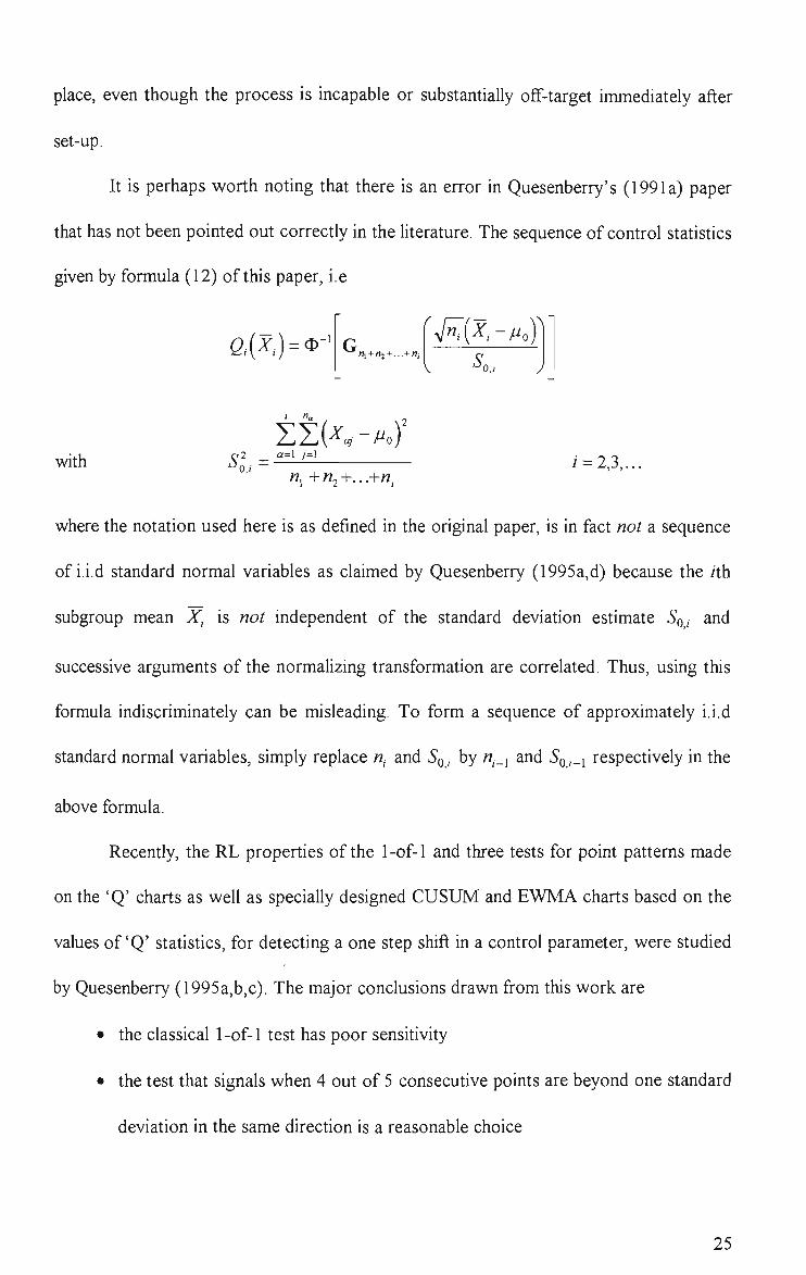
It is perhaps worth noting that there is an error in Quesenberry's (1991a) paper
that has not been pointed out correctly in the literature. The sequence of control statistics
given by formula (12) of this paper, i.e
a(^,)=^-' ni+n2+...+«j
« , (^ , - /^o )
•^0,,
! ««
with ^ 2 _ g=l /=! 'J 0,1 -
SZK-^o) «, + «2 +• • •+«,
/ = 2,3,
where the notation used here is as defined in the original paper, is in fact not a sequence
of i.i.d standard normal variables as claimed by Quesenberry (1995a,d) because the zth
subgroup mean X^ is not independent of the standard deviation estimate ^o, and
successive arguments of the normalizing transformation are correlated. Thus, using this
formula indiscriminately can be misleading. To form a sequence of approximately i.i.d
standard normal variables, simply replace «, and SQ^ by «,_i and 5*0,_i respectively in the
above formula.
Recently, the RL properties of the 1-of-l and three tests for point patterns made
on the 'Q' charts as weU as specially designed CUSUM and EWMA charts based on the
values of 'Q' statistics, for detecting a one step shift in a control parameter, were studied
by Quesenberry (1995a,b,c). The major conclusions drawn from this work are
• the classical 1-of-l test has poor sensitivity
• the test that signals when 4 out of 5 consecutive points are beyond one standard
deviation in the same direction is a reasonable choice
25

• the EWMAQ and CUSUMQ tests are the most sensitive and are about
comparable in overall performance
In accordance with the empirical findings, he also made some recommendations for
practical application. For more insight into 'Q' charting procedures and an interesting
debate of their potential and limitations, see the discussions of these techniques by
Castillo (1995), Hawkins (1995), Farnum (1995), Woodall, Crowder and Wade (1995)
and the response from Quesenberry (1995d).
A logical extension of the 'Q' charting techniques to the control of the mean level
of a multivariate normal process when prior estimates of the process parameters are not
available has also been presented by Tang (1995). The author demonstrated that this
method is particularly useful for 'picking up' a sustained shift in the mean vector when
subgroup data are used.
In fact, this dynamic approach of charting was first perceived by Hawkins (1987).
He proposed two related CUSUM procedures based on transformed individual readings
for checking the constancy of process average and variability, along with some
implementation details and illustrative examples. These were proposed as substitutes for
the standard CUSUM procedures which generally assume known parameters. The
proposed method provides another useful alternative for controUing, particularly, short
run processes as it does not require knowledge of process parameters in advance of
production runs and eliminates the need for a separate preliminary study.
In order to effectively apply the CUSUM procedure, it is well understood that
successive values for which the sum is accumulated should be independent and
identically distributed. For this reason, the following transformation formula (attributable
26

to WaUace (1959)) was suggested to obtain a sequence of independent and
approximately standard normal variables, 2^'s, :-
^/ = 8/-15
U / - 1 3 . (7-2) In 1+ '
2 ^
V 7-2.
where T, = 0-1) A J Aj_^
J V Sj_^ J
Xj : /th individual reading
Xj : mean of the first 7 readings
5^ : standard deviation of the firsty readings
By maintaining a cumulative sum of successive Zj's, starting from the 3rd observation,
and using the established control rule, process mean stability can thus be monitored
progressively without having to wait until adequate process performance data has built
up. However, this method should not be used indiscriminately. Careful examination of
the above transformation formula reveals that the resuhing Zj 's are always positive and
can be regarded as 'folded' standard normal variables which can assume positive values
only. In fact, this normal approximation formula was originally considered by Wallace
(1959) for converting upper tail values of the student-? distribution to corresponding
standard normal deviates. Hence, the need for a modification to the formula is indicated.
The minor change necessary is simply the addition of a negative sign to the transformed
value Zj if 7] is less than zero. For purposes of controUing process dispersion,
Hawkins suggested using the scale CUSUM given in his previous paper (Hawkins
(1981)) which involves cumulative summing of the foUowing quantities :-
27

¥J 0.822
^ 0.349
He made some efforts to justify his recommendation for a 'self-starting' CUSUM
over the adoption of a CUSUM procedure based on some start-up calibration data.
These included consideration of the average run length properties of the two methods.
His simulation resuUs indicate that 'self-starting' CUSUM procedures are superior to
those obtained with some 25 special start-up values, not to mention the short run
situations where usually much less than this is available for initiating conventional cusum
charts.
A final concern about this approach is its likely lack of robustness to both non-
normality and to the presence of outliers in the underlying distribution of process
measurements. Without previous data, there is often no assurance that the process
output will conform reasonably to a normal distribution. The question arises, therefore,
as to what effect departures from the normality assumption wUl have upon performance.
Hawkins (1987) argued, by quoting others' resuUs, that his method works for non-
normal heavy-tailed data with little loss in ARL performance.
The latter issue is particularly pertinent as a sequence of measurements (which
might include occasional outliers) is used simuUaneously both for process control and to
refine parameter estimates. Apparently, incorporating unknowingly occasional valid
extreme observations into the estimates of the process parameters will cause inflation or
deflation of them. This can have a substantial negative impact on the performance of the
control method. To cope with this as well as to protect the CUSUM method (which is
intended primarily for 'picking up' sustained mean shifts of small magnitude) from signals
generated solely by isolated outliers, Hawkins (1987) suggested a robustification
28

approach using 'winsorisation'. 'Winsorizing' the measurements means that any
measurement beyond a preset threshold wiU be set equal to it and used in subsequent
calculations. In this manner, 'winsorisation' reduces or limits the effect of outliers on the
parameter estimates and the properties of the control charts. This idea was further
discussed by Hawkins (1993b) who also examined the relationship between the
'winsorizing' constants for 'self-starting' CUSUM and CUSUM based on a large process
performance study. He stated that this method provides good protection against outliers
with little additional cost in computational effort. In the same paper, he also showed that,
'winsorizing' causes little loss to CUSUM procedures in responsiveness to actual mean
shifts for various sets of clean, contaminated and clean-contaminated data.
Note that, for monitoring process dispersion based on individual observations,
the Exponentially Weighted Mean Squares (EWMS) and Exponentially Weighted
Moving variance (EWMV) by MacGregor and Harris (1993) may be used following
some adaptations. The latter is particularly useful for processes with drifting means when
it is used in conjunction with the conventional EWMA. In the absence of historical data,
these monitoring procedures may be initiated at the 3rd observation where the first two
observations are used to provide some initial estimates of the mean and the standard
deviation, resuhing in some essentially 'self-starting' procedures. Approximate control
limits for the resulting techniques may either be obtained algebraically or by means of
simulation.
2.7 Control Based on Exponentially Weighted Moving Averages
CastUlo et al.(1994) proposed two aUernative methods as improvements to the
'Q' charting technique, for monitoring the deviations from target based on individual
29

measurements where the process standard deviation is assumed unknown. These
methods are based on some exponentially weighted moving average (EWMA) type
control statistics. The first method resuUs from a straightforward adaptation of the
standard EWMA control algorithm with the smoothing factor, X chosen to be 0.1, the
initial value of the EWMA statistic ZQ equated to the specified or known target, / g and
the unknown standard deviation, a estimated sequentially in some suggested manner.
The resuhing EWMA statistic
Z, = (1 - A.)Z,_i + AJr, ,?=1,2,...
is plotted on a control chart with limits
^° \2-X
where & - ' ^ 4
with S,:^X,-Mo, S,= l^j;^(X,-X,y, t = 2,3,. 1=1
C4 is a control chart factor depending on t that can be found from most of the standard
text books on SPC and L denotes a constant that is chosen to achieve specified run
length performance. The authors also noted the use of the more exact transient control
limits (for the rth observation) given by
^io ± ^ 1 A- r, / , , \ 2 f
1 - ( 1 - ^ ) ' <^t 2-?iL
The other control algorithm was derived from the well known Kalman model
(see, for example, Crowder (1989)) upon noting that the assumed i.i.d in-control model
for the process measurements can be represented by a special case of the Kalman model.
The resuhing control statistic is given by the following recursive expression :-
30
Z,=(\-X,)Z,_i+X,X,- Zo=^o
This latter was referred to as the adaptive Kalman filtering control method since the
smoothing factors or Kalman weights, I / 5 change adaptively according to
K-ir^ (2.4)
The variance components of the model, including the process variance, <j^ and the
posterior variance of the process mean after the fth observation, q^-X^o^, are
estimated and updated from the data sequence as follows:-
o-j =i5i , a^ =d^ t = 2,3,...
FoUowing Crowder (1989), the control limits for this method were given as
Mo±L^ (2.5)
The initial value q^ was found to have practically no effect on the ARL performance of
the method provided it is greater than zero. A variant of this method has also been
presented by the same authors (Castillo and Montgomery (1995)) where the of in (2.4)
and L in (2.5) are respectively replaced by 1 and KG^, and K is a constant chosen to
yield specified ARL performance. In the same paper, they provided some guidelines for
the economic design of the control scheme with respect to K and the number of
observations to take in a batch. The objective of the economic model is to minimize the
expected total cost per batch (which comprises sampling/inspection cost, cost associated
with false alarms and cost of running an out-of-control process) subject to certain in-
control run length performance requirements.
31

It was demonstrated using simulation, that for a particular choice of the design
parameters; X, % and L, the first two methods have better ARL performance than the
corresponding 'Q' chart for 'picking up' ofiF-target conditions from start-up, especially
when the size of the deviation (in muUiple of standard deviations), 5 , is small. It was
also found that, these methods (with the particular choice of the design parameters) are
superior to the classical Shewhart chart (classical in the sense that the process parameters
are assumed known) in terms of ARL for small 5 . Furthermore, it was observed that,
using the same criterion, the first control method has a comparable performance to the
classical EWMA chart. Despite these, the choice of the design parameters are quite
arbitrary and no consideration is made of the optimality of the design for these control
techniques. In addition, it is necessary to consider more complete profile of the RL
distributions instead of only the use of ARL (and SDRL) for the reasons given in the
first chapter.
Another contribution along this Une comes from Wasserman (1994) who
proposed the use of the so-called Dynamic EWMA control chart. This technique differs
from the former methods in the charting convention and the manner in which the
variance components are estimated. In particular, the Dynamic EWMA chart compares
the specified target \1Q with the varying control limits (constructed from the posterior
distribution of the process mean) given by
l^Cl^i — ZJ—Lo i-,JX(
UCL, = Z , + Z a , 7 > ^
where Xi= ^ ^' \ . , q, = - q = ^ q,-i+Oi_i l-X
32

a ? = - ^ , a , = a , _ i + l, ^,=^,_,+{\-X)(X,-Z,_,f. a,
An out-of-control condition is signaUed by the chart if the target M-Q is outside these
limits. Note that this is equivalent to plotting and comparing Z, 's with the control limits
Note also that the equations for estimating o^ and q^ are derived from Bayesian
considerations, ag and pg ^^^ the parameters for the chosen Gamma distributional prior
of the precision parameter, -^. X represents the prespecified steady state value of the
o
EWMA smoothing parameter. Wasserman and Sudjianto (1993) developed a similar
technique for detecting the presence of linear trend in process measurements. This is
based on the second order dynamic linear model, 2-DLM (a special case of the Kalman
model) defined by the following observation and system equations :
Observation : System :
where X, and fi, denote respectively the observed value and the process mean of the
quality variable at time t or for the rth sampling inspection unit and b, represents the
level change or trend parameter in the interval [t-\,t]. The observation error, v, and
the random errors in the system equations, Wj, and ^2?' ^^^ assumed to be distributed as
V, ~7V(0,V), w,, ~A^(0,Wi), w^, ~N{0,W,)
where V, Wj and W2 are some constants. As with Dynamic EWMA control chart, the
resulting technique involves charting the varying control limits.
X, = } i , + v , .
^ i r = ^ ^ r - l + ^ - l + ^ l / .
b, = b,_^+W2t,
t = l2 ... 1. - ^ 5 ^ 3 • • •
/ = 1,2,...
t = \,2,...
33

LCL, =ii,-1,^07
UCL, = a r + ^ V ^
and signal the departure of process mean from its in-control value or speficied target p,Q
if these Umits do not enclose [XQ. |J., and Q , in the above expressions are updated
recursively using the following equations :
A/ = Kt^t + ( l -^u) (Ar- i + 4-i)
b, =A,2,(^,- | ir_i) + (l-A-2,)Vi
^i , f -^u
^u+V-^2,r -
^ 3 J
R, + V
Q , r - ^l ,f "^ ' ^2,1 - ^2,t - '^2,t^3,r' Q , f - ^ 2 , / " ^
- ^ 1 / ~ ^I , r -1 + 2C3^,_2 "^ ^ 2 , / - l + ^ l , f ' -^2,f ~ ^2 , f - l + '^2,t' ^3,C ~ ^2,t-\ + ^3 , f - l + ^3 , / -
w,= l f ^ 3 , f^2, . cp (p
ri 1 .0 I
r r ~ •^ l . t - l '-"3,f-l
.Q,f-1 ^2,t-lJ
'1 0
U L
where )i,o=M.o> K-^^ ^^^ ^ ' the so-called discount factor, is chosen to yield
specified ARL performance. CQ is the variance-covariance matrix for the prior
distribution of the vector of process mean and trend parameter and is chosen to reflect
the uncertainty of the prior estimates, [XQ and SQ. If V is unknown, it is suggested
estimating it sequentially using a Bayesian procedure. Using a set of simulated data, the
resuhing technique was shown to be more effective than the classical individual values
chart and the 'Q' chart with known mean and unknown variance for detecting small
process trends. Table 1 of the same paper also indicates that the transient 2-DLM
control charts (with observational variance assumed known) tend to react more quickly
34

to smaU process trends than the steady state 2-DLM and the conventional EWMA
charts.
A control method based on adaptive Kalman filtering, coupled with a tracking
signal feature, has also been proposed by Castillo et al.(1994) as an aUernative to the 'Q'
chart for the case where both ju and CF are unknown. It was noted that besides being
capable of 'picking up' sudden mean shifts, this control procedure can also be used to
detect other out-of-control conditions such as linear process trends. In order to use this
method, some prior estimates of p. (denoted by Jj,^) and a (denoted by a^) are
required. In the short-run environment, reasonably accurate estimates may not be
available. However, it was shown using simulation, that this control technique can
provide better ARL performance than the 'Q' chart especially for early shifts of large
sizes (more than 2 standard deviations) if the estimate of p. differs from the true value
by less than 1.5 standard deviation and a is under or over-estimated by less than 50%.
Again, since the RL distributions for both procedures after the shift are unknown, the
resuhs may not reflect their actual relative performance correctly.
The method involves the computation of the so-called smoothed error statistic
and the smoothed mean absolute deviation, defined respectively as (Trigg and Leach
(1967)) :-
Q(t)=ccelt) + {\-a)Q{t-\); Q[o) = 0
A{t) = a\e, {t)\ + (1 - a)A{t -1); A(0) = 0.8^^ ^2I{2-X,)
where the one-step-ahead forecast error is
and the variance of the process is updated sequentially by
35

T^ \ 2 a',=a&l,+{l-a){x,-X,_,)
For this control technique, a signal is triggered when
>L A(r)
the control limit, L being between 0 and 1.
As the computational effort involved is substantial, implementation of the above
control algorithms requires computerisation. No guidelines about the choice of the
design parameters to achieve desired operating performance are available.
All the methods discussed thus far either ignore or give inadequate consideration
to the problem of process 'warm up', when the process is invariably unstable. On the
other hand, the following approach, which determines the 'control' limits based on given
specifications, appears to be capable of handUng this problem effectively.
2.8 Deriving 'Control' Limits From Specifications
Without the data necessary to set up conventional control charts, compounded by
the problem of process 'warm up', it makes some sense to use product specifications to
provide control information. A control technique that pre-determines its 'control' limits
by reference only to the specifications rather than requiring an accumulation of data for
computation of control Umits, is known as 'pre-control' (PC).
P.C was first proposed by Shainin (1954) as an aUernative to various traditional
on-line quality control methods and, in particular, as an improvement to X and R charts.
It provides a simple and flexible tool for process monitoring as well as set-up approval,
particularly in the low volume manufacturing environment. P.C is conceptually different
from traditional charting techniques in that it focusses directly on preventing non-
36

conforming units from occurring rather than on maintaining a process in a state of
statistical control. The details of operation and the practical merits of this method are
given in Chapter 6.
A new type of control chart which originates from the idea of 'pre-control',
named the 'Balance' chart (B.C) has been introduced by Thomas (1990). B.C can be used
in several different modes. When B.C is used in 'pre-control' mode, it eliminates the
need for estimating the process parameters but instead, derives 'pseudolimits' (±pL) from
the specified tolerance. In B.C, successive measurements from the process on a certain
quality characteristic are classified as -1 , 0 or 1 according to their values relative to ±pL
and specification boundaries. Cumulative recording and plotting of these data about a
target line give information both on the process 'accuracy' and 'precision'. A mathematical
derivation of the control limits which define the maximum deviation of the plot from the
target line, and the maximum number of positive and negative changes from the start of
the run is provided in the same paper. In addition, several rules governing the maximum
number of changes in a given run length were developed to indicate the possible presence
of process troubles. With manual charting, however, too many supplementary rules wUl
complicate the interpretation of the Balance chart.
Besides data scoring, B.C has the unique feature that the operating rules and
control limits are common to every application of the chart. Thus, it has great potential
for computerisation.
Like Pre-Control, this technique does not require exact measurements, but only
needs to know into which 'band' the measurements faU. In order to justify his
recommendation, Thomas also provides comparison of the Balance chart and the X
37

chart operating characteristics for a mean shift of 1 standard deviation, along with some
Ulustrative examples which clearly show that B.C possesses higher sensitivity.
The last two charting methods fallmg m this category were presented by Bayer
(1957) (see also Sealy (1954)) and MaxweU (1953). Both methods are essentially the
same, as they are adaptations of the Nominal X & R charts with limits derived on the
assumption that the process is just capable of meeting the specification. The only
difference between them is that the latter expresses the coded measurements and
'control' limits in terms of'ceUs'.
Representing the specification band by 10 ceUs, the resulting 'ceU' chart has
constant control limits regardless of the specification or the actual process capability,
provided the sample size remains unchanged. Thus, it is possible to have just one chart
per machine on which all parts having possibly different specifications processed can be
controlled. However, these methods of control charting cannot handle one-sided
specification situations.
A comparison between these adjusted X &, R charts and 'pre-control', based on
certain statistical grounds is presented in Chapter 6. The resuUs of the comparison
indicate that the former are superior in many circumstances.
2.9 Adjusting Set-up Continuously Based On Process Output
As a substitute for conventional SPC for low volume production, an entirely
different approach was proposed in Lill, Chu and Chung (1991), 'Statistical Setup
Adjustment' (SSA). This represents a form of'feedback control' where the deviation from
the desired dimension or error of the measured output characteristic, is used to calculate
the best possible adjustment to be made in a machine set-up, starting with the first piece
38

produced. As such, it is not a set-up approval method but one which provides an
algorithm as to how much adjustment should be made as each of the successive
observations arises. Methods are also presented to minimize the number of adjustments,
to avoid early false signals and to anticipate the effects of a known trend such as tool
wear.
As discussed earlier, in the presence of significant set-up variation, Robinson
(1991) and Bothe (1990b) proposed separate monitoring of the set-up processes and
their subsequent runs. If the set-up varies from the desired setting but is within
predictable limits, no machine adjustment is necessary. This is due to the fact that such
corrective action is not only uneconomical, but would probably result in a greater
percentage of defects. SSA differs from this method in that it does not accept the risk of
inaccurate set-up as a consequence of natural set-up variation which inevitably exists, but
is constantly 'forcing' the set-up value to the desired dimension. This approach is,
therefore, in line with Taguchi's idea of quality loss, i.e emphasis is placed on the
uniformity of product quality characteristic about its target value rather than on mere
conformance to specifications.
In SSA, both the machine variations and set-up errors are modeUed with
conceptual normal populations. From available information and experience, a 'maximum
likelihood' estimator of the set-up error can be obtained and hence the correct adjustment
derived. However, determination of the standard deviation of set-up variability based on
subjective judgement, as suggested, leads to doubts about its reUability. In fact, it is
possible to obtain such an estimate directly from the avaUable data.
In this work, the implicit assumption is made that set-up is the critical or
dominant 'system' that largely determines quality of the output. In other words, defects
39

are the direct result of the accuracy of tools or precision of adjustment of the set-up.
Therefore, theoretically, SSA does not provide protection against mean shifts or increase
in process spread due to some special causes during the production run.
If set-up is the dominant cause system, this method works provided the effects of
adjustments are manifested instantaneously and in full. The realization of this, however,
requires dynamic machine control with automatic inspection feedback and measurable
means of adjustment.
2.10 Monitoring Process Input Parameters
By monitoring the process output, traditional SPC and the approaches discussed
above, at best, indicate only when production is not free of troubles. In many instances,
when an out-of-control condition is indicated, numerous corrective measures are possible
and the correct course of action is not always obvious. As such, delay in preventing
waste is inevitable. For smaU lot production, this can be regarded as the same
shortcoming as 'post mortem' inspection !
In view of this Umitation, recent research into the area of applying SPC in low
volume manufacturing environments has given up trying to monitor the process output
but instead has concentrated on the process inputs (Foster (1988) and Thompson
(1989)). Foster presented this idea for controlling highly technical or time consuming
processes where corrective measures for unacceptable work are often uncertain or even
unknown. The implementation strategy for the suggested approach involves the creation
of a 'true' process by compiUng a 'Master Process Requirements List' from all
specifications used for a particular process, selection of the vital few critical input
parameters to be monitored and process capability evaluation.
40

2.11 Economically Optimal Control Procedures
While, traditionally, the development of SPC techniques has been mainly
concerned with statistical efficiency, the ultimate objective of any process control
strategy is cost reduction as a result of reduced scrap, rework and rejects, improved
product quality and increased productivity. This objective may be accomplished by
having an economically optimum policy governing the process monitoring, adjustment
and maintenance activities. In the light of this, over the last four decades, a considerable
amount of study has been devoted to the design of process control methods with respect
to economic criteria. Various process models and cost structures have been proposed
and the corresponding optimal control strategies derived. However, much of the
theoretical work on incorporating cost considerations into the design of process control
procedures has been undertaken implicitly in the context of long production runs.
The economic decision models currently available for on-Une quality control can
be broadly classified into two types. These are economic-process-control models and
economic models for traditional SPC. In their paper, Adams and Woodall (1989)
distinguished between these two types and highlighted some simUarities and differences
between them. A thorough review of the literature on the latter was provided by
Montgomery (1980). Ho and Case (1994) supplemented this work by presenting more
detaUed and complete discussions of different models and aspects of economic design for
traditional SPC, and by summarizing the pubUshed work on economic designs of control
charts covering the period from 1981 to 1991. For typical examples of the former, see
Box and Jenkins (1963), Box, Jenkins and MacGregor (1974), Bather (1963) and
Taguchi(1981).
41
Crowder (1992) considered a short run economic-process-control model in
which observations on a certain measured quality characteristic of the product are
assumed to be generated by an integrated moving average (IMA(1,1)) process and the
costs involved consist of the usual quadratic loss of process mean being off-target and
the fixed cost for each adjustment. He also made the assumptions that any adjustment
made to the process has a known effect (i.e no adjustment error) and that an adjustment
changes the process mean instantaneously or before the next sample measurement is
taken (i.e no process dynamics or inertia). Sampling cost and sampling interval were not
formally considered. Furthermore, deterministic drift and step or cyclical changes were
not taken into consideration.
The proposed model seeks to find the sequence of adjustments, a /5 , which
minimizes the total expected loss, L{n), incurred throughout the production run as given
by the following expression :-
L{n) = ^j Z ( i-"' + c,(5(a,_,)) \
where c^ is the cost parameter associated with any squared deviation of process mean,
//, from target (assumed, without loss of generality, to be 0), c^ represents the cost of
adjustment irrespective of magnitude, n is the terminating sample number and
6{a)=\ ifa^O = 0 ifa = 0
Using dynamic programming or the backwards induction technique, the author
derived an algorithm which enables the optimal control or adjustment strategy (i.e the
optimal sequence of adjustments, a/5) to be obtained numerically. An approximation
formula was also given for the case where the total number of inspections, « < 10 and
42

the cost ratio, c = - ^ > 200. In general, his results can be stated as follows. The resulting ^1
decision procedure as to when and how much adjustment should be made is based on the
Bayes (or Posterior) estimate of the current process mean. It was also found that the
'control' or adjustment Umits are changing with time and becoming wider towards the end
of a production run, in contrast to the fixed limits proposed by some for the asymptotic
case. This solution, he stressed, is consistent with the philosophy of traditional SPC in
that it calls for adjustments only when the process mean is substantially off-target. In
addition, it is found to be intuitively reasonable as the 'widening' action limits will
decrease the UkeUhood of performing economically unjustifiable adjustments or
maintenance near the end of a production run. In the same paper, Crowder
demonstrated, by an example, that using the infinite-run (fixed) limits for the short-run
problem with relatively large adjustment costs can significantly increase the total
expected cost.
Woodward and Naylor (1993) also presented an approach to short run SPC
which takes economic factors into consideration. In this work, a normal linear model is
assumed in which three components of variation are involved. These are the set-up,
adjustment (or resetting) and inherent process variabilities. The model also implies that
there is no delay for any adjustment to take effect, no occurrence of parameter changes
within a machine set-up or production run and that the process standard deviation is
constant irrespective of product types. In comparison to that of Crowder, these authors
proposed a more reaUstic cost structure which includes the foUowing components :
• inspection cost
• rework cost
43

• scrapping cost
• cost associated with adjustment
• quadratic loss of being off-target
They considered a sequential scheme with three possible control actions at each
decision point and attempted to derive a control rule using Bayesian methods such that
the decision made at any stage of the sequential procedure minimizes the expected loss
over aU possible fiiture decisions based on a given cost function. However, the solution
of this optimal control problem is not straightforward and requires the use of techniques
such as backwards induction. As they stated, in practice, it is impossible to find an
optimal rule for this control plan because of the complexity introduced by the three-way
decision structure. In view of this, a simplification in which a control decision is only
made at two stages was considered. Even with this simplified scheme, determination of
the decision boundaries remains compUcated and requires a great deal of numerical
computation.
For both the proposed economic process control models, some prior knowledge
of the process parameters such as the variance terms or availability of some relevant
historical data for their estimation is assumed. Woodward et al. described a method to
quantify the historical information pertinent to their model. In practice, this could be a
problem because historical data for this purpose is rarely sufficient in the short-run
environment.
Another practical problem with these SPC approaches is the difficulty in
specifying the cost parameters. This is due to the fact that some of the cost factors are
intangible. For example, it is difficult to figure out the value of the cost parameters
associated whh the quadratic loss of being off-target and the loss due to process
44

downtime (as a consequence of process adjustment), even by someone who has
substantial knowledge of production and of the cost involved. As a first step to the
implementation of these economic decision models, it is advisable to carry out a
sensitivity analysis of the models to identify the critical parameters and subsequently
exercise greater caution in their determination. However, this is a time-consuming
exercise.
45

CHAPTER 3
MEAN CONTROL FOR MULTIVARIATE
NORMAL PROCESSES i
3.1 Introduction
The majority of the statistical process control (SPC) techniques proposed to date
for controlling the mean of a multivariate process are based on Hotelling's (1947) x^ or
7^-type statistic. Other multivariate control procedures, including the use of principal
components and multivariate cusum (MCUSUM) techniques, were reviewed by Jackson
(1991). A multivariate version of the exponentially weighted moving average chart,
referred to as the MEWMA chart, has also been presented by Lowry, Woodall, Champ
and Rigdon (1992). Apart from these, some techniques that are designed to provide
protection against changes in the process covariance matrix have been presented, for
example, by Montgomery et al. (1972) and Alt and Bedewi (1986). In recent years, some
attempts have also been made to develop control techniques which can both detect
process irregularities and identify the actual set of out-of-control variables, taking into
account the correlational structure of the quality characteristics (see for eg.,
Doganaksoy, Faltin and Tucker (1991), Hawkins (1993a) and Hayter and Tsui (1994)).
All of this work, however, assumes that the process mean, ji and the process covariance
matrix, Y, are known or that they can be reliably estimated prior to fiiU scale production.
Thus, these techniques do not readily lend themselves to applications in the short-run or
^ Part of the material from this chapter is based on the paper entitled 'Mean control for multivariate processes with specific reference to short runs'. Proceedings of the International Conference on Statistical Methods and Statistical Computing for Quality and Productivity Improvement, August 1995, Seoul, Korea.
46

low-volume manufacturing environment where data for estimating the process
parameters are invariably unavailable.
The main thrust of this chapter is to present some 'self-starting' and unified
procedures, for monitoring the stability, and in particular, the mean level of a multivariate
normal process where prior estimates of the process parameters are not available, such as
frequently occurs in short-run, low-volume and multi-product manufacturing
environments. The proposed techniques also facilitate the control of long-run processes
at an earlier stage. For completeness, control procedures are also given for the cases
where \i, E or both are assumed known in advance of the production runs. In addition,
two EWMA procedures specifically designed for detecting sustained mean shifts and
linear trends are considered. These are shown to be superior to some competing
procedures. The total discourse of this chapter is in the context of discrete items
manufacture.
3.2 Methodological Basis
One of the desirable properties for any SPC procedure is that the in-control
behaviour is predictable. This is the case if successive values of the control statistic are
independent realizations of a known constant distribution or at least approximately so
under in-control conditions. Another desirable property is the capacity to use additional
run rules with the associated control chart to help identify any non-random patterns
otherwise not apparent. The control statistics presented in the next section possess these
properties. As the arguments involved in establishing the distributional properties of
these control statistics are similar, this section considers only a particular case, namely.
47
that based on individual observations where the process mean vector and variance-
covariance matrix are unknown prior to production.
Let Xj,X2,...,X^ be independent/7-variate random observation vectors which
have the same covariance structure and are distributed as,
X,. ~A^^(^i^.,2:), j = \,2,...,k
where Z denotes the unknown non-singular variance-covariance matrix. Next, define
V, = X,. - X, 7 = 1,2,...,it
where ^ ; = 1
We wish to test the hypothesis,
Ho: |J . i= | i2= "M-zk = M'(say) vs. H^ : not all |i^'s are equal
Under Hg and the assumption of a constant process variance-covariance matrix.
=K V/f-AfipCuvSv)
where M^V - ^ykpxl Z v ^ Z O C ,
(8> denotes the {left) Kronecker Product (GraybiU (1983), p.216) and
Ck-\ _ J. k k
k k
c =
V k
k
1 k
k-\ k J kxk
Some linear combinations of the pxl component vectors Vi, V2, , V^ that are
uncorrected are now obtained using the standard principal components approach.
Consider the following linear combinations ;
48
Y i = « n V i + a j 2 V 2 + +ai^V^
Y2 =a2iVi +a22V2+ +fl2;kV^
^k = « H V I +a^2V2+ +«^^V^
In matrix notation, these are represented by the following equation
Y = r V = (l(8)A)V
where I isa. px p identity matrix and
(3.1)
A =
«11 «12
^^21 ^^22
... a Ik
V«H ^kkJ kk^ kxk
Thus, the variance-covariance matrix of Y = (Yj^ Y v;) ' i IS
Z Y = r S v r ' ^
= Z<8)ACA . (3.2)
To produce vectors Yj, Yj, ... ,Y^ which are uncorrelated, A in (3.2) is chosen to
diagonalize the symmetric matrix C. One choice for A is
A =
1 4k
1 V2 1
V6 1
V4(4-l)
1 ^ -1 V2 1
V6 1
N/4(4-1)
0
-2 V6 1
V4(4-l)
. . .
. . .
0 -3
N/4(4-1) 0
4k 0
0
0
\ylk{k-l) ^jk(Jc-\)J
where the rows of the matrix are the normalized eigenvectors of C. Substituting A into
(3.1) resuhs in the following linear combinations :
49
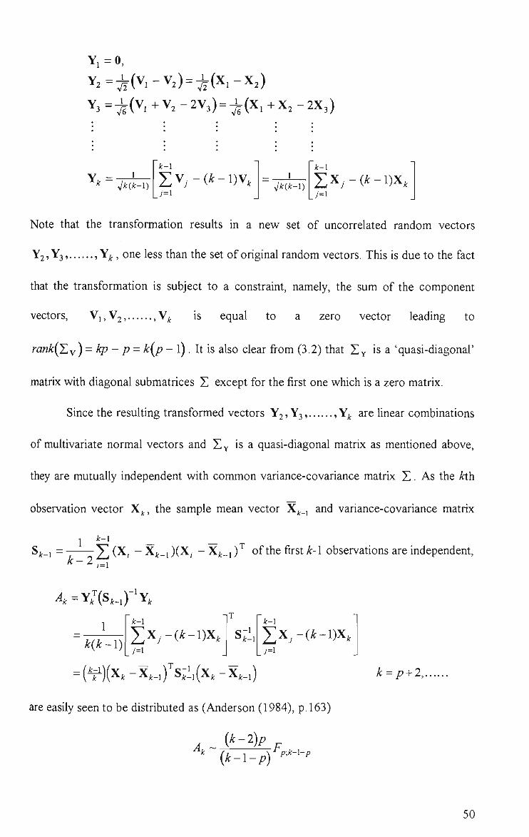
Yi=0, Y2-;^(Vi-V2) = ;^(x,-X2)
Y3=i(Vi+V2-2V3) = -^(X,+X2-2X3)
k ^k(k-l)
k-l
2 V , - ( ^ - l ) V , 7=1
^k(k-l)
k-l
2:X,-(A:-1)X, 7=1
Note that the transformation resuUs in a new set of uncorrelated random vectors
Y2, Y3, , Y^, one less than the set of original random vectors. This is due to the fact
that the transformation is subject to a constraint, namely, the sum of the component
vectors, Vi,V2, ,V^ is equal to a zero vector leading to
rank(Ty)- kp- p = k{p - l) . It is also clear from (3.2) that Zy is a 'quasi-diagonal'
matrix with diagonal submatrices Z except for the first one which is a zero matrix.
Since the resulting transformed vectors Y2, Y3, , Y^ are linear combinations
of multivariate normal vectors and Z y is a quasi-diagonal matrix as mentioned above,
they are mutually independent with common variance-covariance matrix Z . As the ^ h
observation vector X^, the sample mean vector X^_, and variance-covariance matrix
1 *- i _ _ S _i = ^ (X; - X^_i )(X, - X^_i )^ of the first k-\ observations are independent.
k-2 i=\
A-Y^(Sfc-i) Y
1
k{k-\)
k-\
Y^Xj-{k-\)X, 7=1
k-\
J^X^-{k-\)X, 7=1
~ \T')\^k ~ ^k-\) ^k-iy^k ~ ^k-\) k = p + 2,
are easily seen to be distributed as (Anderson (1984), p. 163)
A, {k-2)p
{k-\-p) ^P\k-\-p
50

where F ,i 2 denotes the F-distribution with vl and v2 degrees of freedom. Before
proceeding to show that successive A/^'s are statistically independent, a number of
remarks wUl be made. Note that ^^ is the familiar T^-type statistic that can be used to
check the consistency of X^ as coming from the same normal distribution as the sample
of k-\ preceding observations. This statistic possesses certain optimal properties, as
reported in Anderson (1984, pp.181). Of aU tests whose power depend on
k — l T _i (|i^ -p.) Z~ {[i-ic -\^), the test based on Aj^ can be shown to be uniformly most
powerful for testing the equality of mean vectors of the two normal populations from
which X;. and the sample of k-l preceding observations are drawn, when the unknown
variance-covariance matrix Z is assumed to be constant (see Lehmann (1959)). It can
also be shown, using a theorem of Stein (1956), that this test is admissible i.e, there
exists no other test which is better or uniformly more powerful. Besides, note that the
denominator degree of freedom of theF-distribution associated with Aj^ varies according
to k. If the values of the A/^'s are plotted in different scales, they are likely to give a
misleading visual impression about the status of the process. Thus, it is advantageous to
transform the A,^'s into a sequence of independent and identically distributed variables,
preferably having standard normal distribution, because any anomalous process
behaviour will then show up more clearly in the resuhing control chart. This can also be
assisted by means of additional run rules.
To estabUsh mutual independence of successive Aj^'s, it is first proved that they
are pairwise independent. Clearly,
Y,~Ar^(0,Z), Y,,i~A^^(0,Z), {k-2)S,_,~Wp{k-2,l)
51

are mutually independent. The notation Wp(v,'E) here denotes the p-dimensional
Wishart distribution with v degrees of freedom and parameter Z • Let D be a non-
singular matrix such that DSD = I and define
Y ; = DY, , Yl, = DY,,i , S:_, = DS,_iD^
Thus,
Y ; ~Np(0,1), Yl, ~Np(0,1), {k-2)S;_i ~Wp(k~2,1)
and their independence is preserved. Due to the invariance property of the
transformation.
-^k - Y^ S^_jY^ - Y^ \^k-i) Y^ ,
A - Y ' T S"^Y - Y * ' ^ / ' S * W *
^k+l - '-k+l'^k '-k+l - ^k+\\^k) */fc+l
Noting that (A:-2)S^_i = (A: -1)8^ - Y^Y^ and using an identity for matrix inverses
(Press(1982), Binomial Inverse Theorem, p.23), Aj^ may be expressed as foUows :
A -fc^ •r(s:)"'Y; r(s;)"'Y;
+ (k-l)-Yl\slYYl
As Y^*' (s;^r'Y^* is independent of S; (Srivastava and Khatri (1979), Theorem 3.6.6,
p.94) and Yj^, , it is also independent of any fiinction of S] and Y * j . Thus,
Y^^IS^ j Y^ is independent of A,^^^ = Y^JJS^ j Y +j and it foUows immediately that
A^ (a fiinction of Y^^fs^j Y^) is independent of ^^^,. Similariy, it can be shown that
any pair of A^ 's are pairwise independent. Note that.
52

^k+2 • yt+2 ~^Y^+2J^(« v^jt+Y^^jY^^iJ Y^^
and since Y^^(s]^) Yl is independent of S^ , Y ' , and Y* ^ ' it is clear that A^ is also
independent of ^ . 2 • ^Y induction, A^^^ and A^^„ {m^n)aiQ independent.
Using the result of pairwise independence, it is now possible to proceed to show
that they are mutually independent. As Y^^lsH Y^, S^, Yj , and Y* ^ are mutually
independent, their joint probability density function (p.d.f) is
/(Y;sr'Y;,S;, Y;,„ Y;,2) = g(Yrsr'Y,J/Z(S:)^(Y,;,)Z(Y;,2)
where g,h,q and Z represent their marginal probability density flinctions respectively.
The joint moment generating fimction of
A=Y;X-IY;=/I(Y;X"Y;)
^k+\ - Yyfc+iS^ Y^+1 = j2\^ky^k+\)
A — V*^ S* V * — /" l^ l* V * V * \ ^k+2 - ^k+2'^k+\ *yfc+2 - J 3\^k^ *A:+1' *A:+2J
where / ^ / j and f^ are some fuctions of the indicated arguments, is given by
^4 .4 . . ^ . . . ( 1 > 2, 3) = j .'' ^^^^^-' ^34- 2 (A, A.X, A.2 )dA,dA,,,M,,, all possible
(4.-4^+1,4+2)
where Q(A,^,A,^^^,A,^^^ denotes the joint p.d.f of Aj^, A,^^^ and..4 +2- Integrating over
the original space gives.
53
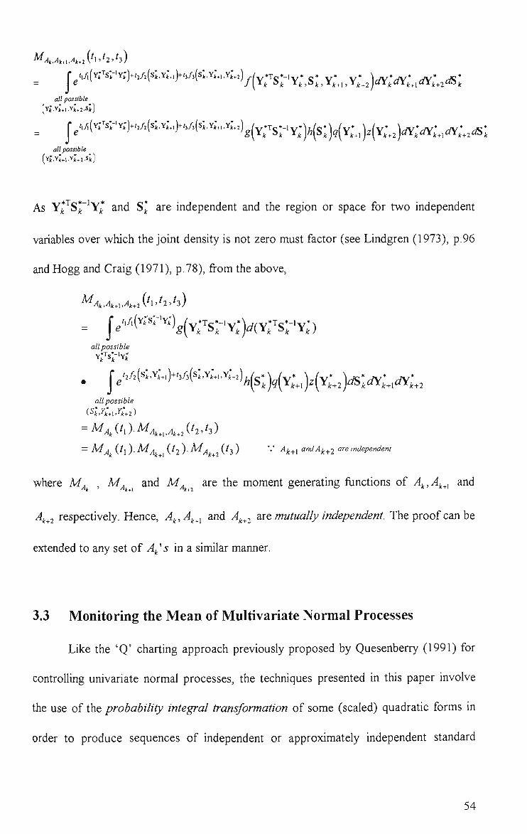
W4,.<,.,./I,.,('l.'2>'3)
^ Je'''('''"'':''''>'-^>(^*-''>-'^''^'(''"''^'"-''")/(Yrs:-'Y;,s;,Y;,Y;,,)<<,<.,<s; all possible
l^,4.^sr^;y.Msi.:..)Msir..,.r..,)^^^^^^^^^ all possible
[-rkyUiyk^z-^k]
As Yj^^Sl 'Y^ and S are independent and the region or space for two independent
variables over which the joint density is not zero must factor (see Lindgren (1973), p.96
and Hogg and Craig (1971), p.78), from the above,
^4A+lA+2(^l'^2,^3)
= j/'^'("^*'*^"'^^*'g(Yrs;-Y;)^(YrsrY;) all possible
all possible
= ^AM)-^A,^uAkJhJ3)
= ^A, i.h )• ^ 4 ^ , ih )• 4 , 2 ( 3 ) *•• \+\ ^"dA,^^2 ""-^ dependent
where M^ , M^ and M^^^ are the moment generating flinctions of A^,Af^^^ and
A^^^ respectively. Hence, Ai^,A^^^ and A^^._ are mutually independent. The proof can be
extended to any set of ^^'5 in a similar manner.
3.3 Monitoring the Mean of Multivariate Normal Processes
Like the 'Q' charting approach previously proposed by Quesenberry (1991) for
controlling univariate normal processes, the techniques presented in this paper involve
the use of the probability integral transformation of some (scaled) quadratic forms in
order to produce sequences of independent or approximately independent standard
54
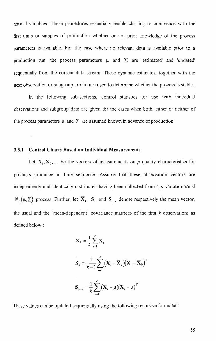
normal variables. These procedures essentially enable charting to commence v^th the
first units or samples of production whether or not prior knowledge of the process
parameters is available. For the case where no relevant data is available prior to a
production run, the process parameters |i and Z are 'estimated' and 'updated'
sequentially from the current data stream. These dynamic estimates, together with the
next observation or subgroup are in turn used to determine whether the process is stable.
In the following sub-sections, control statistics for use with individual
observations and subgroup data are given for the cases when both, either or neither of
the process parameters i and Z are assumed known in advance of production.
3.3.1 Control Charts Based on Individual Measurements
Let Xi,X2,... be the vectors of measurements on p quality characteristics for
products produced in time sequence. Assume that these observation vectors are
independently and identically distributed having been collected from a /?-variate normal
Np[\i,'E) process. Further, let X ., S^ and S^^ denote respectively the mean vector,
the usual and the 'mean-dependent' covariance matrices of the first k observations as
defined below :
« 1=1
i=l
, k
These values can be updated sequentially using the following recursive formulae
55

X,=j[{k-l)X,_,+X,] k = 2,3,.
k ~J7~7\^k-i'^T\^k '^k-i){^k~^k-i) k-3,A,.
k-l S ^ , . - i + | ( X , - n ) ( X , - n f ^ = 2,3, S , ^ ^'^-^ k
Additionally, the following notation will be used ;-
0(«) : distribution function of a standard normal variable
0~^(») : inverse of the standard normal distribution fiinction
xl{*) '• distribution function of a chi-square variable with v degrees of freedom
F^i v2(*) • distribution function of an F variable with vl numerator degrees of
freedom and v2 denominator degrees of freedom.
The appropriate control statistics are now presented as follows:
Case (I) : Both |i and Z known
Z,=^-\xl(T,)] ^ = 1,2,
where T; = (X, - ti)""Z'^X, - n) (3.3)
Case ( n ) : p, unknown, Z known
Z,=0-ypiT,)] k = 2,3,
where T, = ( ^ ) ( x , - X , _ i ) ' z - ^ ( x , -X,_,) (3.4)
56
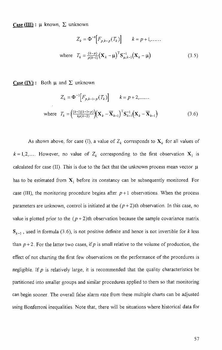
Case (nn : \i known, Z unknown
Z, = cD-^[F,,,_/r,)] k = p + l.
where T, = | ^ ( X , - n ) " s - ; , _ i ( X , - n ) (3.5)
Case (IV): Both p. and Z unknown
Zk=^~'[Fp,k-i-p(T,)] k^p + 2,
where T, = ( i ^ ^ ^ ) ( x , - X , _ , ) ' s ^ ! , ( x , - X,_,) (3.6)
As shown above, for case (I), a value of Z^ corresponds to X^ for aU values of
A: = 1,2,.... However, no value of Z^ corresponding to the first observation Xj is
calculated for case (II). This is due to the fact that the unknown process mean vector \x
has to be estimated from Xj before its constancy can be subsequently monitored. For
case (III), the monitoring procedure begins after p +1 observations. When the process
parameters are unknown, control is initiated at the (p + 2)th observation. In this case, no
value is plotted prior to the (p + 2)th observation because the sample covariance matrix
S _j , used in formula (3.6), is not positive definite and hence is not invertible for k less
than p + 2. For the latter two cases, ifp is small relative to the volume of production, the
effect of not charting the first few observations on the performance of the procedures is
negligible. Ifp is relatively large, it is recommended that the quality characteristics be
partitioned into smaUer groups and simUar procedures appUed to them so that monitoring
can begin sooner. The overall false alarm rate from these muhiple charts can be adjusted
using Bonferroni inequalities. Note that, there will be situations where historical data for
57
estimating the process parameters are available but insufficient for us to assume that the
in-control values of the process parameters, particularly the covariance matrix, are
essentially known. Under these circumstances, such data may be used to provide more
stable estimators and to initiate process monitoring sooner, as considered by
Quesenberry(1991a) for the univariate setting.
It is clear from the preceding section, that {Z^} for each case is a sequence of
independently and identically distributed (i.i.d) normal variables with mean 0 and
standard deviation 1 under the stable in-control normality assumption. The distributional
property obtained for case (IV) is the most pertinent resuU for short run SPC.
As the plot statistics for all cases are sequences of i.i.d. N(p, l) variables, the
resulting control charts can be constructed using the same scale and with the common
Shewhart control Umits ±3. In addition, supplementary run rules can be employed to
reveal any assignable causes hidden in the point patterns of the charts. Although the
argument statistics 7^' s can be plotted instead of the transformed variables Z^' s, this
practice is not recommended because for those cases other than case (I), the use of 7^'5
involves the added complexity of varying control Umits. The use of these procedures is
illustrated later.
3.3.2 Control Charts Based on Subgroup Data
In practice, the use of subgroup data is often preferable to individual
measurements even in situations where only a limited amount of data are available. This
is due to the fact that the resulting control charts are more sensitive to substantial shifts
in the process average and that the subgroup mean (vector) is less affected by departure
from the underlying normality assumption, by virtue of the central limit theorem.
58

Adaptation of the above formulae yields appropriate control statistics for
monitoring the stability of the process mean vector based on subgroup data. Discussion
wiU be restricted to the case of constant subgroup size. Let X, , n and k denote
respectively theyth observation vector of the /th subgroup, the common subgroup size
and the subgroup number, and define the following quantities :
\ "
" 7=1
j = i
7=1
k n
«?'=i^ZZK-*--^y ;=1 7=1
(,_,)s<;-.>+l|;(x,-^)(x,-j.)^ 7=1
/=1
where S[ ° = ^plud - ^ • ^^^ ^^^^ technique is now appUed to transform the sample
mean vectors X ,)' s to standard normal variables for each of the cases considered above
for individual measurements.
Case (I): Both p, and Z known
Z,=0-\xl{T,)] k = l,2,.
59

where T, = n[x^,^ - M)"I.-\x^k) ' n) (3.7)
Case (ID : \x. unknown, Z known
Zk=^-Yp{T,)] k = 2X
where T,=[^){^^,^-%,_,^\-'^^,^-%_^ (3.8)
Case (DT) : p. known, Z unknown
Two alternative techniques which employ different process covariance matrix
estimates will be considered for this case. The first one incorporates |LI into its 'running'
estimate of Z whereas the other ignores knowledge of p and is based on the pooled
estimate S '2,ed. It wiU be seen in section 3.5 that the latter gives better run length
performance.
(a) Uses p. in estimation of Z
Zi=4>-'[iV,„(j_,>.^,(rj)] i = 2,3, r,>p
where T, = ( ^^g fe f )(x<„ - n ) \ s t ' ^ ) - \ \ , , -^) (3.9)
(b) Uses Pooled Sample Covariance Matrix
Z,=<I.-'[/v„„_,^,„(?;)] k = \.2, ,n>p + \
where T, = [^lig=S^](x<„ - ^.)^(s« ) - ( x , „ -^) (3.10)
60
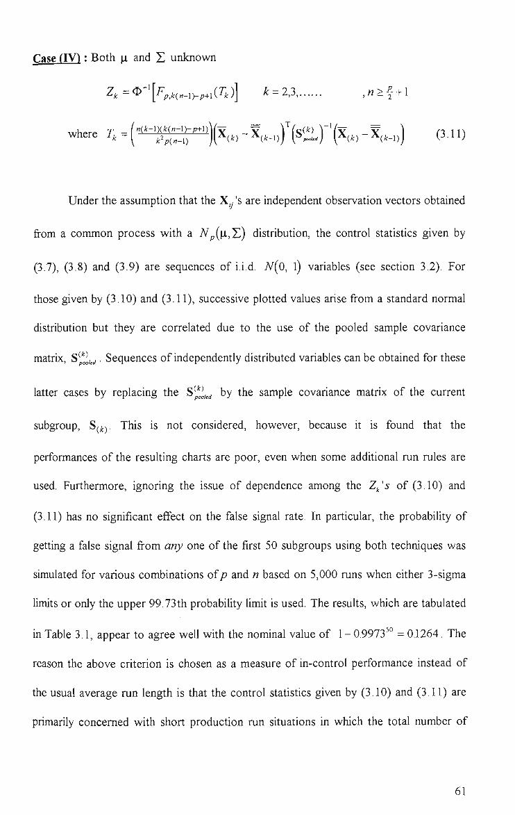
Case (TV) : Both p and Z unknown
Zk=^~'[FpMn-iyp.i(T,)] k = 2,3, , « > f + l
where T, = ( " ^ " ^ y r r " 1 ( ^ ( ^ ) -^(^- ' ) ) ' (^^^-)"(^(^) '^i^-^) ^'''^
Under the assumption that the X, 's are independent observation vectors obtained
from a common process with a 7Vp(p,Z) distribution, the control statistics given by
(3.7), (3.8) and (3.9) are sequences of i.i.d. N(0, l) variables (see section 3.2). For
those given by (3.10) and (3.11), successive plotted values arise from a standard normal
distribution but they are correlated due to the use of the pooled sample covariance
matrix, S^ , . Sequences of independently distributed variables can be obtained for these
latter cases by replacing the S ' , ^ by the sample covariance matrix of the current
subgroup, S(^). This is not considered, however, because it is found that the
performances of the resulting charts are poor, even when some addUional run rules are
used. Furthermore, ignoring the issue of dependence among the Z .'5 of (3.10) and
(3.11) has no significant effect on the false signal rate. In particular, the probability of
getting a false signal from any one of the first 50 subgroups using both techniques was
simulated for various combinations ofp and n based on 5,000 runs when either 3-sigma
limits or only the upper 99.73th probabUity limit is used. The results, which are tabulated
in Table 3.1, appear to agree well with the nominal value of 1 - 0.9973^° = 0.1264. The
reason the above criterion is chosen as a measure of in-control performance instead of
the usual average run length is that the control statistics given by (3.10) and (3.11) are
primarily concerned with short production run situations in which the total number of
61

samples rarely exceeds 50. Furthermore, note that for case (IV), h is possible for each
individual sample covariance matrix to be of less than fuU rank provided the (common)
sample size is not less than y +1 . This is because for the pooled covariance matrix,
^^pliied to be distributed as a positive definite scaled Wishart matrix such that F is well
defined, the total degrees of freedom for the k possibly rank deficient sample covariance
matrices that form S^^^^^, k{n-1) must be at leastp, or equivalently, n>j + l (see
Sullivan et al.(1995)). For this condition to hold for aU k, starting from k = 2, the
minimum sample size is thus « = y +1 where [•] denotes the greatest integer function.
A remark should be made about the computation of the argument statistics for
(3.3) to (3.11) above which involve evaluation of the inverse of a matrix. In fact, each of
these arguments can be expressed as a quotient of two determinants, thus eUminating the
need for inverting either the known process covariance matix or some estimates of it (see
for example, Morrison (1976), p. 134). For instance, the argument statistic of (3.6) has
the following alternative expression
cj (k-lXk-1-p) (^ V V Y ^k-l + kp(k-2) \^k ^k-l)\^k
k 1
-x«)' J _ _ 1
Evaluating an expression of this form is much more convenient than that of its original
form especially when the number of quality characteristics,/? is large.
For some general guidelines on using the above control charting approach,
readers are referred to the article by Quesenberry (1991a) from which the ideas of this
present work originate.
62
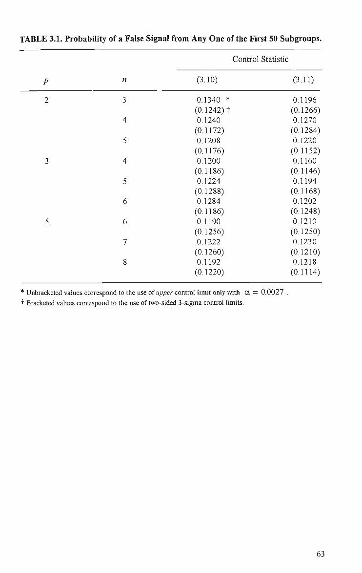
TABLE 3.1. Probability of a False Signal from Any One of the First 50 Subgroups.
Control Statistic
n (3.10) (3.11)
2 3 0.1340 * 0.1196 (0.1242) t (0.1266)
4 0.1240 0.1270 (0.1172) (0.1284)
5 0.1208 0.1220 (0.1176) (0.1152)
3 4 0.1200 0.1160 (0.1186) (0.1146)
5 0.1224 0.1194 (0.1288) (0.1168)
6 0.1284 0.1202 (0.1186) (0.1248)
5 6 0.1190 0.1210 (0.1256) (0.1250)
7 0.1222 0.1230 (0.1260) (0.1210)
8 0.1192 0.1218 (0.1220) (0.1114)
* Unbracketed values correspond to the use of upper control limit only with a = 0.0027 . t Bracketed values correspond to the use of two-sided 3-sigma control limits.
63

3.4 Examples
In this section, use of the proposed techniques are illustrated by some numerical
examples based on simulated data as weU as using data from a previously published
article. The examples presented here are not mtended to cover all possible situations,
however, they provide some insight into the behaviour of the proposed techniques under
various circumstances.
Example 3.4.1
The first illustration uses the formulae for individual measurements. 30
observations have been generated from a bivariate normal distribution with the following
parameters
AO' ( I 1.275 H U5;
z= U.275 2.25J
These data are shown in Table 3.2, along with the computed values of the control
statistics (3.3) to (3.6). The corresponding control charts have also been constructed as
shown in Figures 3.1(a) to 3.1(d). It should be noted that the use of 3-cr control limits in
this and subsequent examples is merely for the purpose of Ulustration. In practice, it may
be preferable to use nartower control limits or only the upper control limit in line with
the traditional Hotelling T^ charting approach.
Note that for the cases with some unknown parameters, the corresponding
statistics were computed using the values of p and Z as given above. Note also that
since p = 2, calculations of the plotted values of the control statistics (3.4), (3.5) and
(3.6) have been started with the 2nd, 3rd and 4th observations respectively. As shown in
the figures, none of the plotted points exceed the control limits for each of the control
64
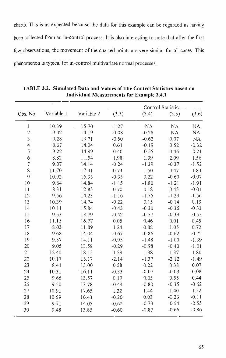
charts. This is as expected because the data for this example can be regarded as having
been coUected from an in-control process. It is also interesting to note that after the first
few observations, the movement of the charted points are very similar for aU cases. This
phenomenon is typical for in-control multivariate normal processes.
TABLE 3.2. Simulated Data and Values of The Control Statistics based on Individual Measurements for Example 3.4.1
Obs. No.
1 2 3 4 5 6 7 8 9
10 11 12 13 14 15 16 17 18 19 20 21 22 23 24 25 26 27 28 29 30
Variable 1
10.39 9.02 9.28 8.67 9.22 8.82 9.07
11.70 10.92 9.64 8.31 9.56
10.39 10.11 9.53
11.15 8.03 9.68 9.57 9.05
12.40 10.17 8.41
10.31 9.66 9.50
10.91 10.59 9.71 9.48
Variable 2
15.70 14.19 13.71 14.04 14.99 11.54 14.14 17.31 16.35 14.84 12.85 14.23 14.74 15.84 13.79 16.77 11.89 14.04 14.11 13.58 18.15 15.17 13.00 16.11 13.57 13.78 17.65 16.43 14.05 13.85
(3.3)
-1.27 -0.08 -0.50 0.61 0.40 1.98
-0.24 0.73
-0.35 -1.15 0.70
-1.16 -0.22 -0.43 -0.42 0.05 1.24
-0.67 -0.95 -0.29 1.59
-2.14 0.58
-0.33 0.19
-0.44 1.22
-0.20 -0.62 -0.60
Cnntrnl Statistir
(3.4)
NA -0.28 -0.62 -0.19 -0.55 1.99
-1.39 1.50 0.22
-1.80 0.18
-1.55 0.15
-0.30 -0.57 0.46 0.88
-0.86 -1.48 -0.98 1.98
-1.37 0.22
-0.07 0.05
-0.80 1.44 0.03
-0.73 -0.87
(3.5)
NA NA 0.07 0.52 0.46 2.09
-0.37 0.47
-0.60 -1.21 0.45
-1.29 -0.14 -0.36 -0.39 0.01 1.05
-0.62 -1.00 -0.40 1.37
-2.12 0.38
-0.03 0.55
-0.35 1.40
-0.23 -0.54 -0.66
(3.6)
NA NA NA
-0.32 -0.21 1.56
-1.52 1.83
-0.07 -1.91 -0.01 -1.56 0.19
-0.33 -0.55 0.45 0.72
-0.72 -1.39 -1.01 1.80
-1.49 0.07 0.08 0.44
-0.62 1.52
-0.11 -0.55 -0.86
65
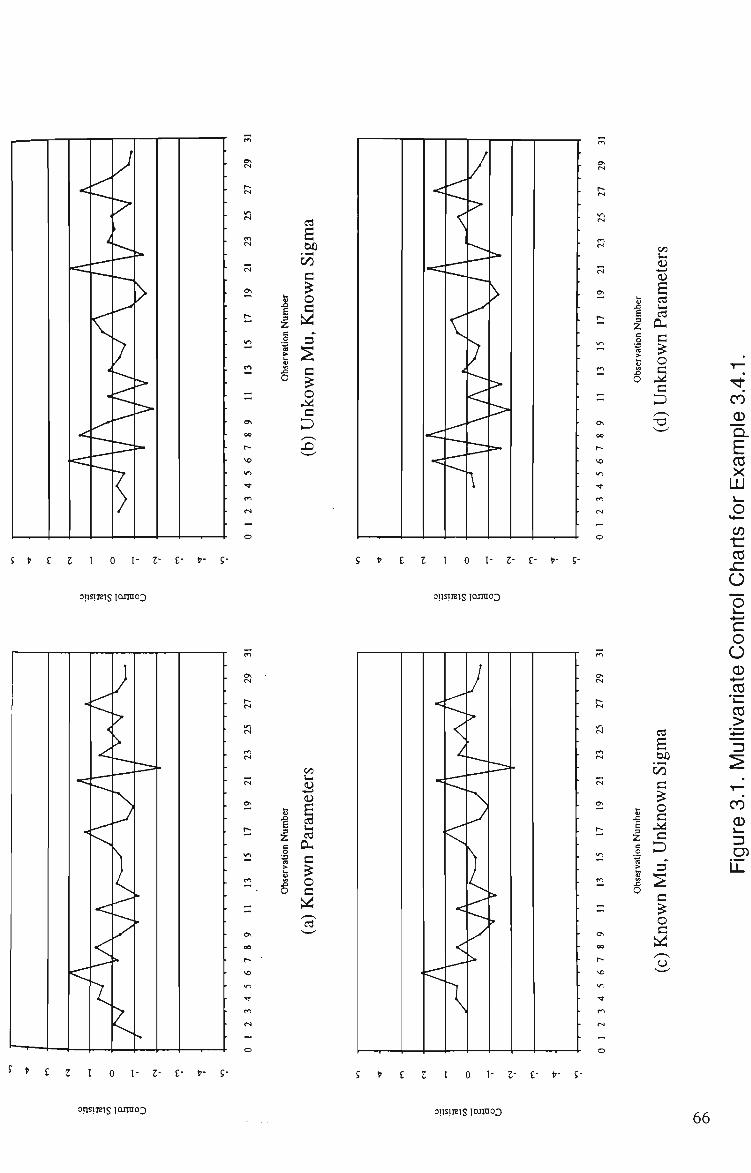
I
B
a o
o a
e a-c o
c D
5 * £ Z I t-- 5- S t £ Z I 0 1- t- £- t-- S-
opsiiBis lOJinoo oijsiiEjs lorrooo
a
A H :?! e
ati
erv
J3
o
o ^ W( cd
OH
a ^ o c
c3
C
o c c
c o c
^ * £ Z I 0 I- Z- £- S t £ t I 0 1- I- £• t- S-
oilsijBis lannoo cijsiiEjs 10Lnno3 66

Example 3.4.2
Next, in order to demonstrate the behaviour of the control charts based on
subgroup data for a stable process, 120 observations have been generated from a
trivariate normal distribution with
^ =
^ 5 ^
12
U5; and Z =
^0.0625 0.10625 0.05^
0.10625 0.25 0.136
^ 0.05 0.136 0.16 y
These observations are grouped into samples of size n = A and the corresponding values
of the control statistics (3.7), (3.8), (3.9), (3.10) and (3.11) are calculated and plotted in
Figures 3.2(a) to 3.2(e). Note that except for the case with known parameters and when
the statistic (3.10) is used, charting begins with the 2nd subgroup.
Again, as shown in the figures, the point patterns of the resulting control charts
are similar after the first few points. This similarity in the point patterns will generally be
the case for other in-control processes and the appearance of the control charts will be
more simUar as the subgroup size increases. FoUowing Quesenberry's (1991) suggestion,
since p and Z are not likely to be known precisely, the safer approach to charting is to
use (3.6) and (3.11) which do not assume known values for the process parameters.
67
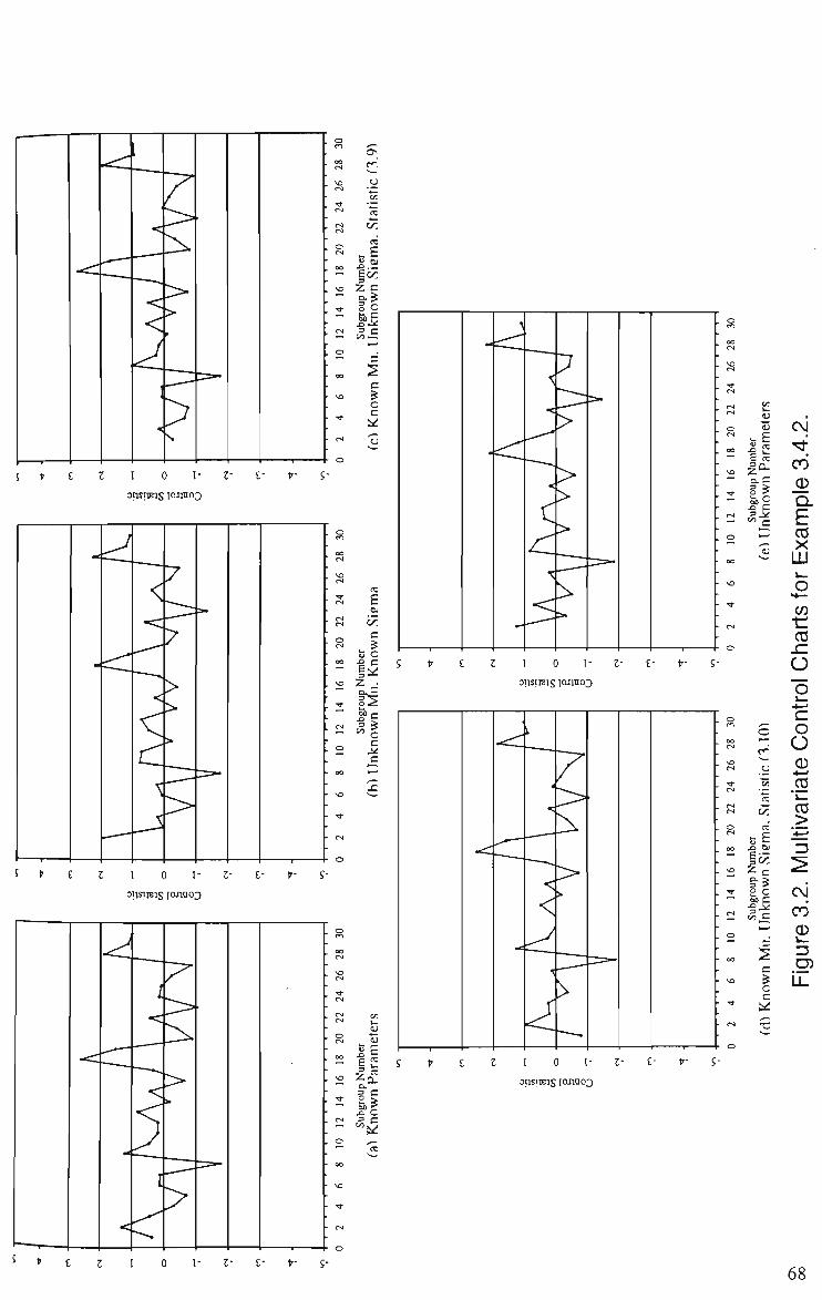
I 0 i-
otjsijejs lojjnoo
I 0 T- Z-
IE •2 re ^^ o g x> C .2 C
( N aj 4)
E re
^ s ^ — oo ^
SO
I 0 I-
3IJSIJBJS lOflnoo
J I 0 I-
CM
CO
_g) Q. E X
LU
CO •c CO
o "o V—
• 4 — '
c o O 03
CC >
CM
CO
CD
68

Example 3.4.3
In this example, two charts are shown in order to compare the control techniques
based on subgroup data for the cases when the parameters p and Z are assumed
known and when they are both unknown. Figures 3.3(a) and 3.3(b) show these control
charts for 30 samples of 3 observations each from a bivariate process where the mean of
the 1st variable increases by 1.5 standard deviations after the 8th sample. The first 8
samples were generated from a A''2(p,Z) process distribution with
A 10>
and Z = U3J
^ 0.25 0.375^
1 0.375 1 ;
whereas samples 9 to 30 were simulated from iV2(p„g^,Z) where
\^, '10.15^
. 23 ,
Note that the correct values of p and Z to use for computing statistic (3.7) are
those before the shift occurs. The figures show that whilst the shift is large enough to
trigger out-of-control signals from both charts as soon as subgroup 9 is observed, that
based on unknown parameters gradually settles into a pattern indicative of in-control
conditions. This is due to the fact that the corresponding control statistic utUizes the
current data stream to estimate the unknown values of the process parameters
sequentially, causing the effect of parameter changes to 'dilute' as more out-of-control
data are incorporated into the parameter estimates. It should be noted, that if an outUer
or out-of-control observation (or subgroup) is present, that observation should be
removed from subsequent computations. If this is not done, the parameter estimates wiU
be distorted, causing an out-of-control process to appear in-control or vice versa.
69

</) (/)
m O CO
OS CS
0 0 (S
> <N
cs CO CS
<N
, ( S
o CN
Os
0 0
r-^ — t
SC
i n
- • *
—"* CO
^ (S '"' f-H
o '""' ON
0 0
r-
so
>n
• *
CO
<N
s ^ E s Z & p 2 3
CD ^^ 0 E CO i _ CO CL c ^ o c ii:
co" ^ CO CD
^amm
D . E CO X LU
L—
o <4— tr CO
SI O "o 1 _
"c o O 0)
.? CO >
"B ^
s CO CO
S t' £ 3 I 0 I- 3- £- t - g-LL
•1 ^ o
S t' £ 3 1 0 I- 3- £- t" S-
^ CO
O CO
oe CJ
r~ cs so cs m ( S
CO CN
CN <N
<N
O CS
ON
OC
r-
so
i r i
• *
CO
CS
;l^ o
OS
0 0
C--
so
w-1
Tj-
CO
cs
—
o
3
z & 3
2
3 00
o 0)
E 2 CO CL c ^ o c ^ c
• i .
CO '^'
CO CD Q .
E CO X LU o
**— •c CO
O
2 c o O CD
CO
CO >
3 ^
g CO CO CD
13 D3
ii.
opsTj^S lOJquoQ OTJSpBlS I0DU03
70
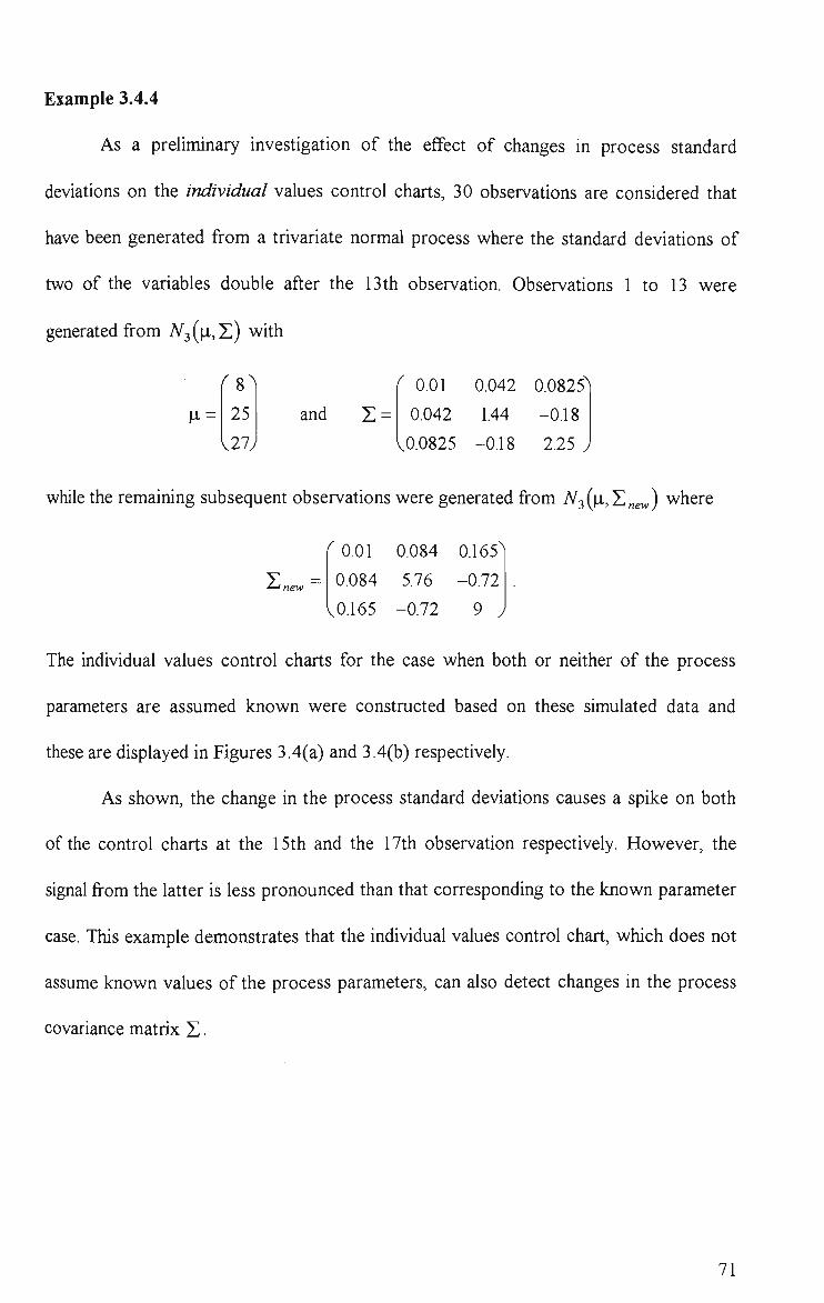
Example 3.4.4
As a preliminary investigation of the effect of changes in process standard
deviations on the individual values control charts, 30 observations are considered that
have been generated from a trivariate normal process where the standard deviations of
two of the variables double after the 13th observation. Observations 1 to 13 were
generated from A''3(p,Z) with
^i = 25
.27>
and Z = ^ 0.01 0.042 0.0825"
0.042 1.44 -0.18
V0.0825 -0.18 2.25 y
while the remaining subsequent observations were generated from N^{yi,Y.r,ew) where
^ 0.01 0.084 0.165^
0.084 5.76 -0.72
^0.165 -0.72 9 ;
The individual values control charts for the case when both or neither of the process
parameters are assumed known were constructed based on these simulated data and
these are displayed in Figures 3.4(a) and 3.4(b) respectively.
As shown, the change in the process standard deviations causes a spike on both
of the control charts at the 15th and the 17th observation respectively. However, the
signal from the latter is less pronounced than that corresponding to the known parameter
case. This example demonstrates that the individual values control chart, which does not
assume known values of the process parameters, can also detect changes in the process
covariance matrix Z •
71

0 1 2 3 4 5 6 7 8 9 10111213 1415 1617 18 19 20 2122 23 24 25 26 27 28 29 30 31
Observation Number
Figure 3.4(a). Multivariate Control Chart for Example 3.4.4, Known Parameters.
72
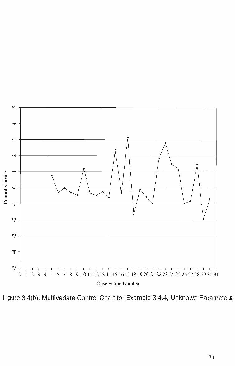
0 1 2 3 4 5 6 7 8 9 1011 1213 1415 1617 18 19 20 2122 23 24 25 26 27 28 29 30 31
Observation Number
Figure 3.4(b). Multivariate Control Chart for Example 3.4.4, Unknown Parameter. .
73

Example 3.4.5
To illustrate the usefulness of individual values control procedure for the
unknown parameters case, consider the data analysed by Holmes et al.(1993) which
gives the composition of 'grit' manufactured by a plant in Europe. These data are
reproduced in Table 3.3 where the columns headed L, M, and S show the percentage
classified as large, medium and small respectively, for each of the 56 observations. Since
the percentages sum to 100 and the sample variance-covariance matrix wUl not be
invertible under this condition, we analyse the data in the first two columns only, as
Holmes et al. did, using a technique based on statistic (3.6). The computed values of this
statistic are provided in the same table and the associated control chart is shown in
Figure 3.5. Note that, as opposed to Holmes et al.'s retrospective testing for process
stability based on all these 56 observations, the proposed charting is done essentially in
real time i.e it begins as soon as the 4th observation is avaUable. Thus, this approach has
the potential to react to process instability sooner than the former method.
As shown in the figure, a signal is triggered by the 26th observation which,
according to Holmes et al., actually occurred in the presence of process troubles. This
observation is thus deleted from subsequent computations. To stress this point, the
charted points corresponding to this and the next observation are disconnected. Although
the plotted point for the 45th observation which was also affected by some identified
special causes does not exceed the 3-a control limUs, using the common run rule that
signals when 2 of 3 consecutive points exceed 2- a limits (in this case ±2) on the same
side of the center line, the process trouble is detected as soon as the next observation is
available. This additional rule provides enhanced detection capability with little loss in
the in-control RL performance, especially for short run situations (refer to Palm (1990)
74

for the in-control RL probabilities of the combined test above). It is, in fact, the ability to
recognise many anomalous point patterns through, for instance, the use of such
additional run rules that the strength of the proposed charting technique lies.
75

Table 3.3. Holmes and Mergen (1993)'s Data and Values of Statistic (3.6).
i
1 2 3 4 5 6 7 8 9 10 11 12 13 14 15 16 17 18 19 20 21 22 23 24 25 26 27 28 29 30 31 32 33 34 35 36 37 38 39 40 41 42 43 44 45 46 47 48 49 50 51 52 53 54 55 56
L
5.4 3.2 5.2 3.5 2.9 4.6 4.4 5 8.4 4.2 3.8 4.3 3.7 3.8 2.6 2,7 7.9 6.6 4 2.5 3.8 2.8 2.9 3.3 7.2 7.3 7 6 7.4 6.8 6.3 6.1 6.6 6.2 6.5 6 4.8 4.9 5.8 7.2 5.6 6.9 7.4 8.9 10.9 8.2 6.7 5.9 8.7 6.4 8.4 9.6 5.1 5 5 5.9
M 93.6 92.6 91.7 86.9 90.4 92.1 91.5 90.3 85.1 89.7 92.5 91.8 91.7 90.3 94.5 94.5 88.7 84.6 90.7 90.2 92.7 91.5 91.8 90.6 87.3 79 82.6 83.5 83.6 84.8 87.1 87.2 87.3 84.8 87.4 86.8 88.8 89.8 86.9 83.8 89.2 84.5 84.4 84.3 82.2 89.8 90.4 90.1 83.6 88 84.7 80.6 93 91.4 86.2 87.2
s 1 4.2 3.1 9.6 6.7 3.3 4.1 4.7 6.5 6.1 3.7 3.9 4.6 5.9 2.9 2.8 3.4 8.8 5.3 7.3 3.5 5.7 5.3 6.1 5.5 13.7 10.4 10.5 9 8.4 6.6 6.7 6.1 9 6.1 7.2 6.4 5.3 7.3 9 5.2 8.6 8.2 6.8 6.9 2 2.9 4 7.7 5.6 6.9 9.8 1.9 3.6 8.8 6.9
2,
NA NA NA 0.6399 -0.4774 -1.4148 -2.0361 -0.1776 2.7482 -1.1743 -0.7038 -1.3520 -1.0359 -0.8824 0.5530 0.2870 1.4587 1.4113 -1.3677 0.6618 -0.7556 -0.2284 -0.4814 -0.5848 0.8209 3.2867* 2.0908 1.4377 1.0241 0.3840 -0.4525 -0.6524 -0.2495 0.3005 -0.3970 -0.7454 -1.6929 -1.9147 -0.7932 0.5805 -0.9938 0.2369 0.3382 1.3784 2.4500 2.0966 0.7397 -0.3457 0.6670 -1.1449 0.3555 1.4025 0.8303 -0.2968 0.4030 -1.4174
* This observation is removed from computation of subsequent Z , ' S.
76
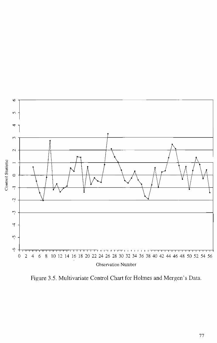
0 2 4 6 8 10 12 14 16 18 20 22 24 26 28 30 32 34 36 38 40 42 44 46 48 50 52 54 56
Observation Number
Figure 3.5. Multivariate Control Chart for Holmes and Mergen's Data.
77

Example 3.4.6
To see how the control technique with unknown parameters that is based on
subgroup data performs in comparison to an existing method, consider the data given by
Alt et al.(1976). These authors presented formulae to compute the control limits for the
r^-type control chart based on a small number of subgroups, both for retrospective and
fiiture testing of the mean level of a muhivariate normal process and used the data to
illustrate the use of these so-called small sample probability limits. The data consists of
measurements on /? = 2 quality characteristics which are grouped into subgroups of size
« = 10. Due to Umited space, the summary data are not reproduced here. However, for
ease of comparison, the values of the T^-type statistic, the stage 1 (retrospective) and
stage 2 (future) control limits are given in Table 3.4, together with the results obtained
using the technique (3.11) proposed in this paper. Note that the stage 1 and stage 2
control limits are set at a = 0.001 and a = 0.005 respectively.
As shown in the table, the use of the proposed technique also results in an
abnormally large value of the control statistic for subgroup 4 as when Alt et al.'s method
is used, indicating that the process was out-of-control when this sample was taken.
Similarly, subgroup 8 is also detected as being out-of-control using both control
procedures.
78

TABLE 3.4. Values of Alt et al.'s Test Statistic, Small Sample Probability Limits and Control Statistic (3.11) for Example 3.4.6.
Subgroup No.
1 2 3 4 5
Subgroup No.
6 7 8 9 10 11 12
Alt et al.'s Stage 1 Statistic
0.009 1.147 0.136 4.901* 0.632
Alt et al.'s Stage 2 t Statistic
0.392 0.197 4.594* 0.190 0.226 0.410 0.460
Stage 1 UCL
1.3268 1.3268 1.3268 1.3268 1.3268
Stage 2 UCLJ
1.5906 1.5906 1.5906 1.5906 1.5906 1.5906 1.5906
Revised Value of Altetal's
Statistic
0.327 0.264 0.034 NA
0.057
Revised Stage 1 UCL
0.9546 0.9546 0.9546
0.9546
Control Statistic (3.11)
NA 1.0758
-1.4909 5.0192*
-0.5821t
0.7766 0.5906 4.8528* 0.4045t 0.3248 1.0596 0.9490
* These numbers exceed their respective UCLs indicating the presence of assignable causes. t These and subsequent values are calculated after removing the out-of control subgroups immediately
preceding them. J These are based on subgroups 1, 2, 3 and 5.
79

3.5 Control Performance
It is shown in Appendix (A.l), (A.2) and (A.3), that the statistical performance
of the techniques presented above depend on the foUowing parameter(s) (scalar, vector
or matrix) for each of the given types of process changes (besides the change point r, i.e
the observation or sample after which the change takes place) :
(a) A sustained shift in the mean vector from p to p„ ,. whilst Z remains unchanged
'^ = i{\i-r,e^-V)^^ \\i-new-V)
(b) A sustained shift in covariance matrix from Z to I] „c,, whilst p remains unchanged
Eigenvalues, X^,...,Xp, of Z„^S"^ or Z"'Z„e^
(c) A simuhaneous sustained shift in mean vector from p to p„ . and covariance matrix
from E JQ_E^
Ti = S"H^i„^-li) and Q = Z " ' E _ Z ^ '
Note that Z ' here denotes the symmetric square root matrix of Z such that
Y. = l}l? (Johnson and Wichern (1988), p.51) and Z"^ = (z^J . The importance of
these resuUs is clear when one realizes that the effort for determining the control
performance of the proposed techniques is greatly reduced. For instance, in order to
determine the performance under the first type of process change, U may be assumed,
without loss of generality, that p = (0,0,..,,0) , Z = I and p„^ subsequently
80

considered in the form of \i„^ ={X,0,...,0) for various values of X. Note that X is
sometUnes referred to as the noncentrality parameter (eg., Lowry et al.(1992)). Some
issues of importance regarding the use of X are discussed in the same paper (see also
PignatieUo and Runger (1990)).
In this section, we will consider only the simplest type of process change, namely,
a persistent change in the process mean vector. The performance of the proposed
techniques are evaluated on the basis of probability of detection within m = 5 successive
observations or subgroups by means of simulation. This is chosen as the performance
criterion instead of the common measure of ARL because, as demonstrated in the
examples using simulated data, the first few observations or subgroups after the change
are the critical ones. If the mean shift is not detected within the first few observations or
subgroups after its occurrence, it is even more unlikely that this will be 'picked up' by
subsequent observations or subgroups because of the 'diluting' effect. In addition, the run
length distributions for the techniques wUh some unknown parameters are not geometric,
so ARL is not a suitable performance criterion (see Quesenberry (1993,1995d)).
Furthermore, this paper is particularly concerned with short production runs or low
volume manufacturing and as such early response of the techniques to any process
anomalies or irregularities is a crucial factor.
It should be pointed out that only an upper control limit is used in the simulation.
This approach is used because the control techniques are intended primarily for 'picking
up' changes in the mean vector and U appears that any such change is likely to resuU in
unusually large values for the control statistics. In practice, however, it might be
preferable to use both lower and upper control limits because the former can provide
protection against occasional changes in the variance-covariance matrix and other
81
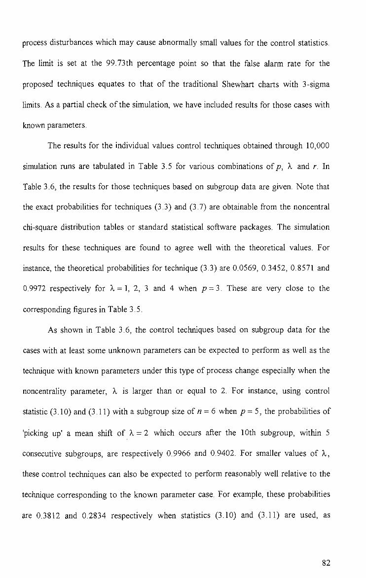
process disturbances which may cause abnormally small values for the control statistics.
The Umit is set at the 99.73th percentage point so that the false alarm rate for the
proposed techniques equates to that of the traditional Shewhart charts with 3-sigma
limits. As a partial check of the simulation, we have included results for those cases with
known parameters.
The resuhs for the individual values control techniques obtained through 10,000
simulation runs are tabulated in Table 3.5 for various combinations of p, X and r. In
Table 3.6, the results for those techniques based on subgroup data are given. Note that
the exact probabilities for techniques (3.3) and (3.7) are obtainable from the noncentral
chi-square distribution tables or standard statistical software packages. The simulation
results for these techniques are found to agree well with the theoretical values. For
instance, the theoretical probabilities for technique (3.3) are 0.0569, 0.3452, 0.8571 and
0.9972 respectively for X = l, 2, 3 and 4 when /? = 3. These are very close to the
corresponding figures in Table 3.5.
As shown in Table 3.6, the control techniques based on subgroup data for the
cases with at least some unknown parameters can be expected to perform as well as the
technique with known parameters under this type of process change especially when the
noncentrality parameter, X is larger than or equal to 2. For instance, using control
statistic (3.10) and (3.11) with a subgroup size of « = 6 when /? = 5, the probabUities of
'picking up' a mean shift of A, = 2 which occurs after the 10th subgroup, within 5
consecutive subgroups, are respectively 0.9966 and 0.9402. For smaller values of X,
these control techniques can also be expected to perform reasonably well relative to the
technique corresponding to the known parameter case. For example, these probabilities
are 0.3812 and 0.2834 respectively when statistics (3.10) and (3.11) are used, as
82

compared to 0.4513 for the known parameter case. As for control based on individual
observations, those techniques with some unknown parameters have poor performance
relative to that based on known parameters when X and r are small and p is large.
However, the performance of these individual values control charts improves with
increasing value of X and r. As shown in Table 3.5, the probability of detecting a shift of
A, = 5 for a bivariate process within 5 successive observations using statistic (3.6), which
does not assume known values for the process parameters, is 0.8514 if r = 20. Apart
from these, a number of points can be noted from the tables. It is found that except for
control statistic (3.10), the proposed techniques decline in performance according to the
number of unknown parameters on which they are based. Specifically, those based on
known values of the process parameters have the best performance as expected, followed
by those with unknown mean vector p , those with unknown covariance matrix Z and
those whh both process parameters unknown. Note also that, for the same A, and r, the
performance of the individual values control techniques become worse as p increases.
Finally, it can be seen from Table 3.6 that using statistic (3.10) is always better or as
good as statistic (3.9) although the former ignores knowledge of p in the estimation of
83

TABLE 3.5. Probability of Detection Within m-5 Subsequent Observations.
Control Statistic
(3.3) (3.4) (3.5) (3.6)
6
10
20
10
20
10
20
10
20
10
20
10
20
2 3 5 2 3 5 2
3 5
2 3 5 2 3 5 2
3 5 2 3 5 2 3 5 2 3 5 2 3 5 2
3 5 2
3
5
0.0720 0.0537 0.0417 0.0736 0.0545 0.0403 0.4430 0.3437 0.2500 0.4357 0.3456 0.2508 0.9153 0.8550 0.7477 0.9124 0.8533 0.7530 0.9993 0.9966 0.9880 0.9994 0.9960 0.9900
1 1 1 1 1
0.9999
1 1 1
1
1 1
0.0492 0.0399 0.0306 0.0588 0.0432 0.0345 0.2560 0.2033 0.1428 0.3230 0.2525 0.1830 0.7050 0.6014 0.4752 0.8074 0.7220 0.5920 0.9687 0.9354 0.8762 0.9921 0.9796 0.9456 0.9996 0.9982 0.9930
1 1
0.9988 1 1
0.9998
1
1
1
0.0328 0.0260 0.0197 0.0437 0.0363 0.0267 0.0807
0.0553 0.0342 0.1660 0.1172 0.0755 0.1887 0.1191 0.0570 0.4011
0.2863 0.1747 0.3735 0.2483 0.1026 0.7040 0.5624 0.3576 0.6114 0.4292 0.1560 0.9096 0.8122 0.5866 0.8180 0.6304 0.2624 0.9862
0.9500 0.8094
0.0245
0.0223 0.0172 0.0367 0.0304 0.0247
0.0541 0.0364 0.0228
0.1353 0.0925 0.0614 0.1325 0.0827 0.0408 0.3314
0.2333 0.1385 0.2728 0.1967 0.0722 0.6213 0.4837 0.2962 0.4880 0.3076 0.0984 0.8514 0.7366 0.5074 0.6980 0.4832 0.1568
0.9702 0.9162
0.7468
84
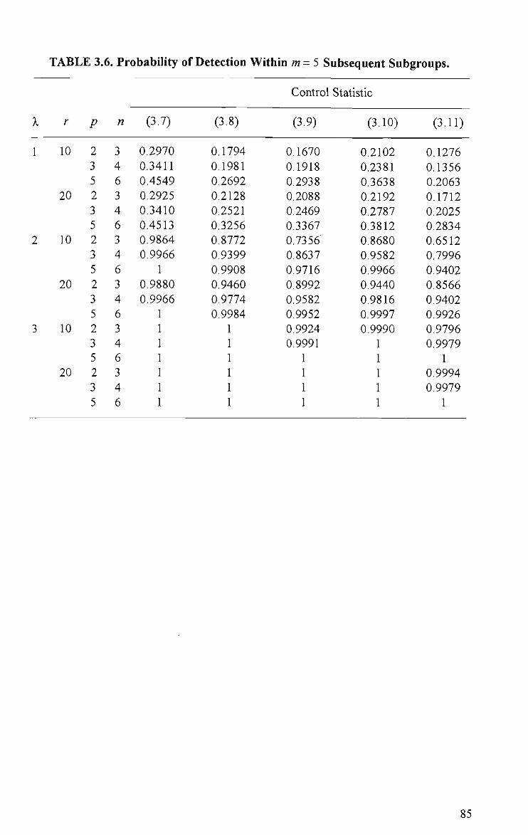
TABLE 3.6. Probability of Detection Within m = 5 Subsequent Subgroups.
X r
I 10
20
2 10
20
3 10
20
P
2 3 5 2 3 5 2 3 5 2 3 5 2 3 5 2 3 5
n
3 4 6 3 4 6 3 4 6 3 4 6 3 4 6 3 4 6
(3.7)
0.2970 0.3411
0.4549 0.2925 0.3410 0.4513 0.9864
0.9966 1
0.9880 0.9966
(3.8)
0.1794
0.1981
0.2692 0.2128 0.2521 0.3256 0.8772 0.9399 0.9908 0.9460 0.9774 0.9984
Control Statistic
(3.9)
0.1670
0.1918 0.2938 0.2088 0.2469 0.3367 0.7356 0.8637
0.9716 0.8992 0.9582 0.9952 0.9924 0.9991 1 1 1 1
(3.10)
0.2102
0.2381 0.3638 0.2192 0.2787 0.3812 0.8680 0.9582
0.9966 0.9440 0.9816 0.9997 0.9990
(3.11)
0.1276
0.1356 0.2063 0.1712 0.2025 0.2834 0.6512 0.7996 0.9402
0.8566 0.9402
0.9926 0.9796 0.9979
1 0.9994
0.9979 1
85
3.6 Detecting Step Shifts and Linear Trends Using A Robust
Estimator of Y and EWMA
As demonstrated by examples 3.4.4 and 3.4.5, when a sustained shift in a process
parameter occurs, the technique presented for the unknown parameter case that is based
on subgroup data wiU either 'pick up' the process change within the first few samples or
it will not signal at all due to the effect of mcorporating out-of-control observations in
the estimation of the process variance-covariance matrix, Z . The latter event is likely to
occur when the shift takes place early in the production and the shift size (as measured
by A) is smaU. This problem is particularly acute when the corresponding individual
values control technique is used.
Apart from one-step shifts, there are situations where the process mean vector,
p changes linearly with time or with the chronological order of the observations or
samples. A linear trend in the multivariate observations is defined by Chan and Li (1994)
as the event which occurs when there exists a constant/7-dimensional vector P such that
PP is a linear function of the sample or observation number. As a special case of this, a
linear trend that occurs after the rth observation is represented by
X , = p , + 8 ,
where p , = j ^ ^~ ''"'^ (3.12) ^ ' [p + /0 i = r + l,... ^ ^
0 and 8,'5 denote respectively a constant vector characterising the linear trend and the
i.i.d Np(0,'E) vectors of random errors. This is the model that is considered herein. If
the linear trend occurs soon after the commencement of production, the control
procedures for the unknown Z case, particularly those based on individual observations
86
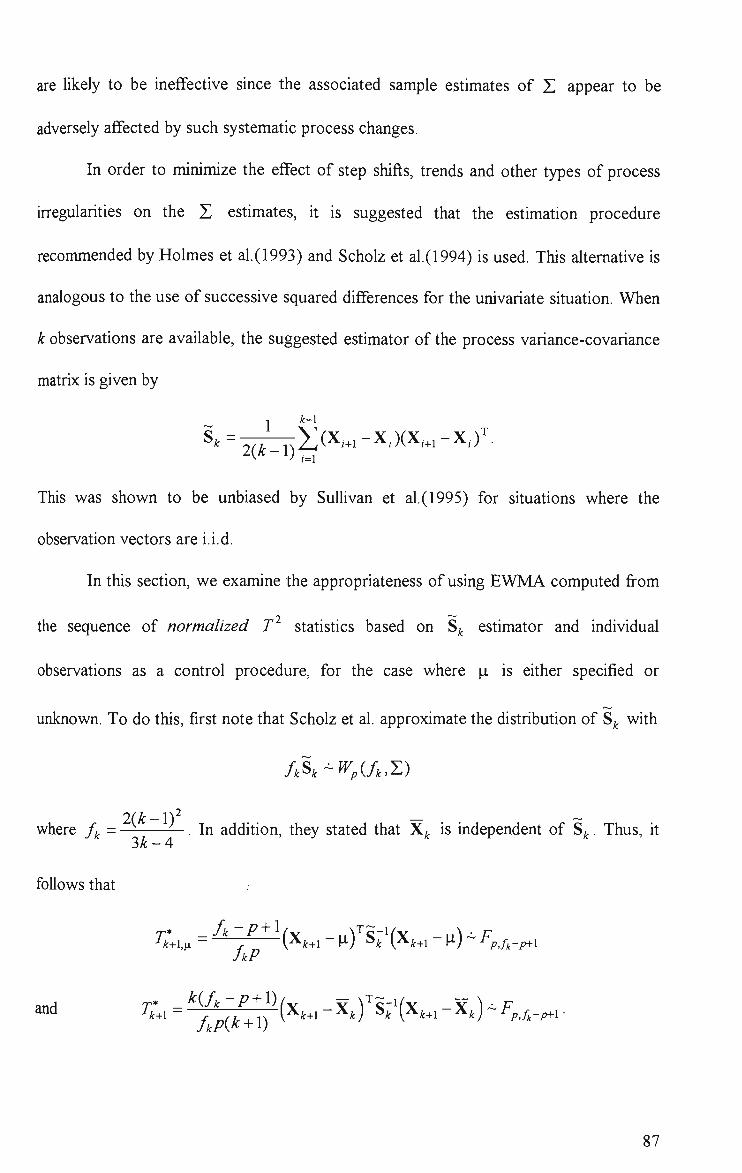
are likely to be ineffective since the associated sample estimates of Z appear to be
adversely affected by such systematic process changes.
In order to minimize the effect of step shifts, trends and other types of process
irregularities on the Z estimates, it is suggested that the estimation procedure
recommended by Holmes et al.(1993) and Scholz et al.(1994) is used. This aUernative is
analogous to the use of successive squared differences for the univariate situation. When
k observations are available, the suggested estimator of the process variance-covariance
matrix is given by
^'"2(ri)^^^'^^"^'^^^'^^~^'^^-
This was shown to be unbiased by Sullivan et al.(1995) for situations where the
observation vectors are i.i.d.
In this section, we examine the appropriateness of using EWMA computed from
the sequence of normalized T statistics based on S^ estimator and individual
observations as a control procedure, for the case where p is either specified or
unknown. To do this, first note that Scholz et al. approximate the distribution of S^ with
fk^k-^Wpif^Y)
where /^ = — —. In addition, they stated that X^ is independent of S^. Thus, it 3k-4
follows that
^k+i,ii - 7 v^k+i ~ M'j ^k V^k+i ~\^)'^ Fp,fk-p+\
87

Note also that the Tj^^^'s (and Tj^'s) are approximately independent when k becomes
large. Thus, as in section 3.3, these statistics can be transformed to sequences of
approx/'/wafe/y i.i.d standard normal variables [zlA and fz^j as follows:
and z; = 3'-[f,,,._,_^,(r;)].
It is now possible to form EWMA statistics with Zl^^ and Z^ taken as the inputs. The
resulting techniques for the known and unknown p case are based on the EWMA
statistics, EWMAZl^ and EWMAZIU^, given respectively by
EWMAZl^ = yZl^ + (1-Y)EWMAZ1^_I
and EWMAZ lUfc = yZ; + (1 - y )EWMAZ lU^_i.
For ease of subsequent discussion, these techniques are referred to as EWMAZl and
EWMAZIU respectively. Note that using these procedures, process monitoring begins
with the kth observation where EWMAZl^_i and EWMAZ lU^_i are set to 0 and k is
the smallest integer greater than . The values of EWMAZl^
and EWMAZIU^ are plotted on a chart whh control limits at ±h.yJy/(2-y) where the
smoothing constant y and the control limits factor h are chosen to achieve specified in-
control run length performance. Using the resuUs obtained by Quesenberry (1995a),
these design parameters are set to 0.25 and 2.9 respectively to give the control limits at
±1.096. These same EWMA parameters are used in all the work reported subsequently
in this chapter. This combination of y and h gives an in-control ARL of 372.6 and an
ARL of 5.18 for a shift of 1.5 standard deviation in the mean of a normal variable. Since
88
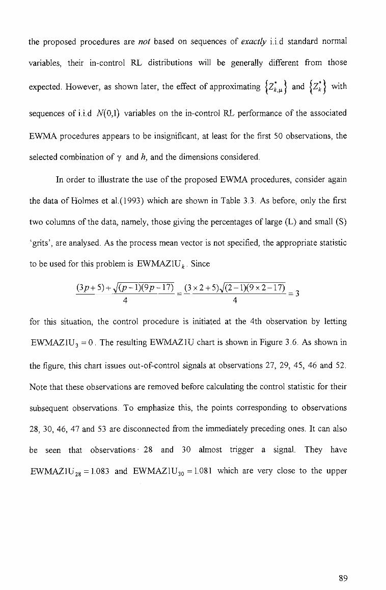
the proposed procedures are not based on sequences of exactly i.i.d standard normal
variables, their in-control RL distributions wUl be generally different from those
expected. However, as shown later, the effect of approximating \Z].A and |Z^ | with
sequences of i.i.d A''(0,1) variables on the in-control RL performance of the associated
EWMA procedures appears to be insignificant, at least for the first 50 observations, the
selected combination of y and h, and the dimensions considered.
In order to illustrate the use of the proposed EWMA procedures, consider again
the data of Holmes et al.(1993) which are shown in Table 3.3. As before, only the first
two columns of the data, namely, those giving the percentages of large (L) and smaU (S)
'grits', are analysed. As the process mean vector is not specified, the appropriate statistic
to be used for this problem is EWMAZIU^. Since
(3p+5) + V(p-l)(9/7-17)^(3x2 + 5)V(2^nO(9x2-17)^^
for this situation, the control procedure is initiated at the 4th observation by letting
EWMAZIU3 = 0 . The resulting EWMAZIU chart is shown in Figure 3.6. As shown in
the figure, this chart issues out-of-control signals at observations 27, 29, 45, 46 and 52.
Note that these observations are removed before calculating the control statistic for their
subsequent observations. To emphasize this, the points corresponding to observations
28, 30, 46, 47 and 53 are disconnected from the immediately preceding ones. It can also
be seen that observations- 28 and 30 almost trigger a signal. They have
EWMAZIU28 = 1083 and EWMAZIU3Q =1.081 which are very close to the upper
89

u
—r
• O
VD
i n
<N wo
o wo
00
O
OO
m VD
m
CO
(N m O m
oo CN
\o
C ^ C N
O (N
OO
o
- 00
- \o
- -rf
- (N
O
I
t-i
I C3 O
00
o
CO ^—> CD
Q co" Cf) O )
C/3
"c CD
CD ^
•D C CO CO CD
E o I
tr CO
O
N <
LU
CD
CO
CD
IJL
niZVIAIAVH 90

control limit of 1.096. In comparison to the use of statistic (3.6) (see Example 3.4.5) and
the retrospective tests of Holmes et al. and Sullivan et al.(1995) using the S,^ estimator,
there are more signals from the EWMAZIU chart for this set of data. These findmgs are
not surprising since it was found by Sullivan et al. that the difference between the mean
vectors of the first 24 and the last 32 observations are statistically significant (an
evidence of a shift in the process mean vector foUowing the 24th observation), while the
'within' variance-covarince matrices are not statistically different.
Next, to see how the proposed procedures respond to linear trends, 50 bivariate
observations have been generated from the process model (3.12) with k = I, p = 0,
1 = 1 and 0 = (0.3,0)"^. Besides EWMAZl and EWMAZIU charts, M charts
specifically designed by Chan et al.(1994) for detecting such process changes have also
been constructed based on the same data. These are aU shown in Figure 3.7. The latter
procedures are developed based on projection pursuit and linear regression techniques.
These procedures involve charting the values of certain statistics based on moving
samples of t/observations. In this example, the size of the moving samples used is d=7.
If p is specified, the sequence of control statistics involved is given by
M t = — T ; V^—^^ , k = d,d+l,...
where W is a <i-dimensional vector wUh the /th element being ,
2
G^ = (X^_^ i - p , ••• X ^ - p ) ^ , U ^ = G J G ^ and d>p. The values of M^ are
plotted on a chart with upper control limit at Fp,d-p,a > ^^^ upper lOOath percentUe of an
F distribution with p and d-p degrees of freedom. If the process mean vector is
91
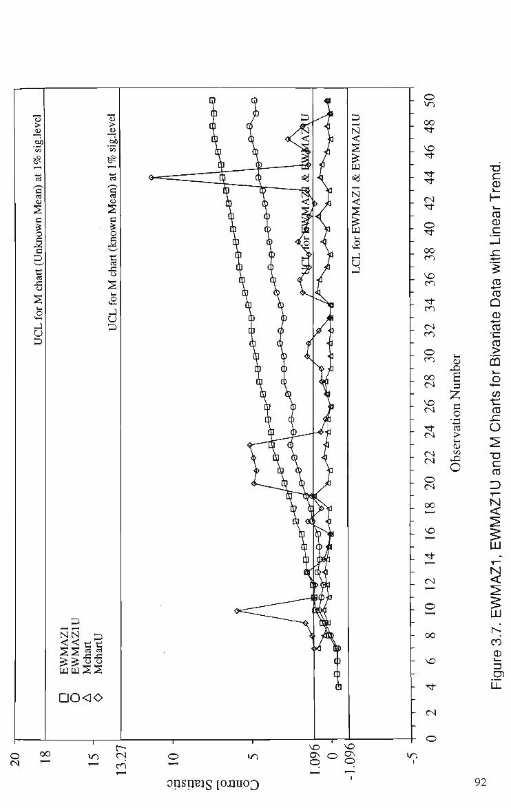
• o c CD
CO CD
c
t-( <D qui
3 Z,
ati
01]
> ^ WD
X )
o
CO •*—' CO Q CD ^ ^ CO k .
CO >
no o
H —
rts
Cha
^ T3 C CO
D —
N <
LU
N <
LU
CO
opspB^s |oxino3 92
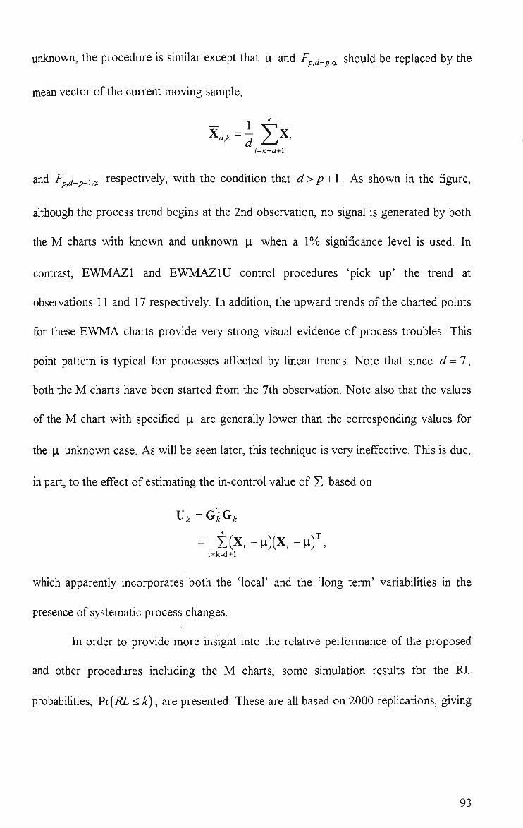
unknown, the procedure is similar except that p and Fpd^p^^ should be replaced by the
mean vector of the current moving sample.
k
i=k-d+l
- J_ d
and Fpd-p-ia respectively, with the condUion that d>p + l. As shown in the figure,
although the process trend begins at the 2nd observation, no signal is generated by both
the M charts with known and unknown p when a 1% significance level is used. In
contrast, EWMAZl and EWMAZIU control procedures 'pick up' the trend at
observations 11 and 17 respectively. In addition, the upward trends of the charted points
for these EWMA charts provide very strong visual evidence of process troubles. This
point pattern is typical for processes affected by linear trends. Note that since d=7,
both the M charts have been started from the 7th observation. Note also that the values
of the M chart with specified p are generally lower than the corresponding values for
the p unknown case. As wiU be seen later, this technique is very ineffective. This is due,
in part, to the effect of estimating the in-control value of Z based on
= i(x,-p)(x,-pf, i=k-d+l
which apparently incorporates both the 'local' and the 'long term' variabilities in the
presence of systematic process changes.
In order to provide more insight into the relative performance of the proposed
and other procedures including the M charts, some simulation results for the RL
probabUUies, ?T{RL < k), are presented. These are all based on 2000 repUcations, giving
93

^ , ^ 10.5(1-0.5) a maximum standard error of J — = 0.0112 which occurs when the probabUity
being estimated is actually 0.5. For the case where p is assumed known, two other
procedures similar to EWMAZl, abbreviated hereafter as EWMAZ2 and EWMAZ3
respectively are considered. The first uses the EWMA computed from the Z^' s of (3.5)
whereas the other is based on the EWMA computed from the following sequence of
statistics :
Zk = ^~' ^P,k-\-p (7(Ff| ('^-^)^^»(''-^)' k = p + 2,.... (3.13)
As for the case with unknown p , a similar EWMA procedure with the Z ' s of (3.6)
taken as inputs is also considered. For convenience, this technique is referred to as
EWMAZ2U.
For a linear trend that occurs immediately (i.e. r = I), the simulated run length
probabilities are shown graphically in Figures 3.8 to 3.13 for A: = 1(1)50 and various
combinations ofp and the trend parameter X^^^^ =yjQ^ H ^ 0 . In fact, using the similar
arguments as that for a step shift, it can be shown that the statistical performance of all
the control procedures considered above depend on A g„ under linear trend conditions
as specified in (3.12). Note that the run lengths here are measured from the 1st
observation although several observations are necessary for initiating the stated
procedures. Note also that statistical comparison of various control techniques can be
misleading if their in-control RL distributions differ considerably. However, as shown in
Figures 3.8(a) to 3.10(a), the difference between the in-control RL distributions for
EWMAZl, EWMAZ2 and EWMAZ3 are practically insignificant for k = 1(1)50 andp =
2, 3 and 5. The same is true for EWMAZIU and EWMAZ2U (see Figures 3.11(a) to
94
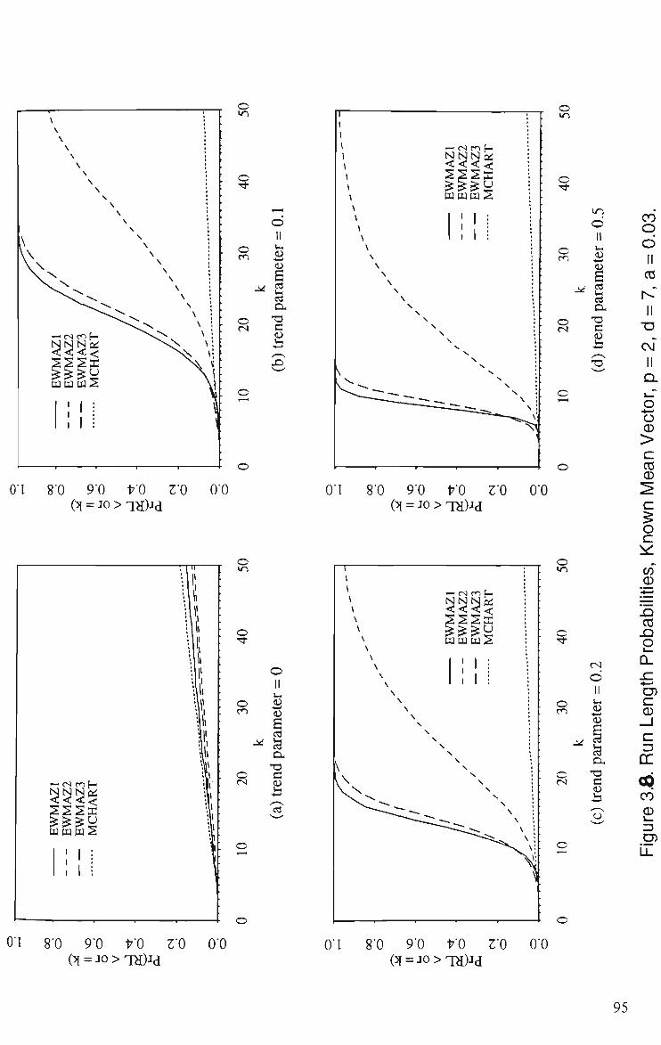
o
O
o en
M
O CS
-2 <u S cd
a OH
TS c (U is
o
o
o
o
s V cd
0"l 8"0 9"0 VO 3'0 (5[ = JO > 'Pi)Jd
O'O 0"l 8"0 9"0 t 'O TO (:5{ = JO > Ta)-id
O'O
o
o
o en
o
s
T3 C 4)
cd
I
\
V \ \ \ \ \ \
>
\ . \
V \ \^^^v.
-H cs m H
^ ^ ^ § i S S S S : 1 ^ ^ ^ • U Q Q D U S :
\ t t •
' ; : 1
1 1 . :
\ ! • s I •
\ ! •
s I • \ 1 •
s 1 •
\ ! s. ;
S ',
\ 1 X !
\ 1 \ ; \ ; . N ;
^—~~^^-» .^ \ ' —^ ^ ~a ^ •
^ * S ^ \',
X
o
o Ti
ro o
O H
8 0 9"0 t 'O Z"0 (5[=J0>T^)Jd
0"0 0"l 8"0 9"0 VO to (5I=J0>T^)Jd
00
95

o
o
o en
^
o (N
O .4—>
u £ a c
TD C g j U l
o
O
10 o II
(—1 (-I
k> cd
" Jd
o -a
8"0 9"0 t7"0 r'O (^ = JO>TH)Jd
0"0 O'l 8"0 9-0 VO Z"0 (5[ = JO > TH)Jd
O'O
o
o Ti-
0 en
^
0 CS
0 e c3 u OH
-a c (U l-l
cd
8"o 90 i7-o ro (^ = jo>TH)Jd
O'O O'l 8'0 9'0 t 'O to 00
96
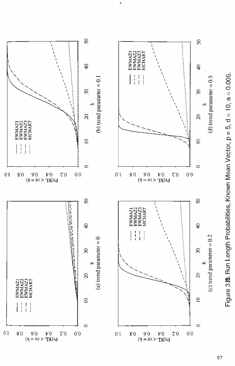
-H fsi m E-H
o IT)
o
o en
M
O r5
(U B
ara
ex -o c (U -b
O'l 8'0 9'0 VO ZO (5l = J0>1H)Jd[
O'O
o
o
o en
M
O cs
«-i
fi cd ^ o-
T3 C3 lU
cd
-^ es en H \
O
o
\r\
30
ter =
0.
<u B •^ 1
O H
o "S cs C
?
in o o o 11 CO
o" • * "
II T3
O'l 8'0 9'o VO ro (5{ = JO > TH)Jd
O'O
in
o
o U-)
o "*
o en
M
O CS
o
cs O II ir! D o Id cd
O H
-o a <u i3
o
O CD
>
now
n M
ean
i^
bilit
ies,
CO
o QL
sz •*—> U) c: CD
_J C 3
CL m
^^ ^^ CO
ure
en "Li.
O'l 8'0 9'0 r o Z'O (31 = JO > TH)Jd
O'O O'l 8'0 90 17'0 Z'O (51 = JO > iH)Jd
00
97
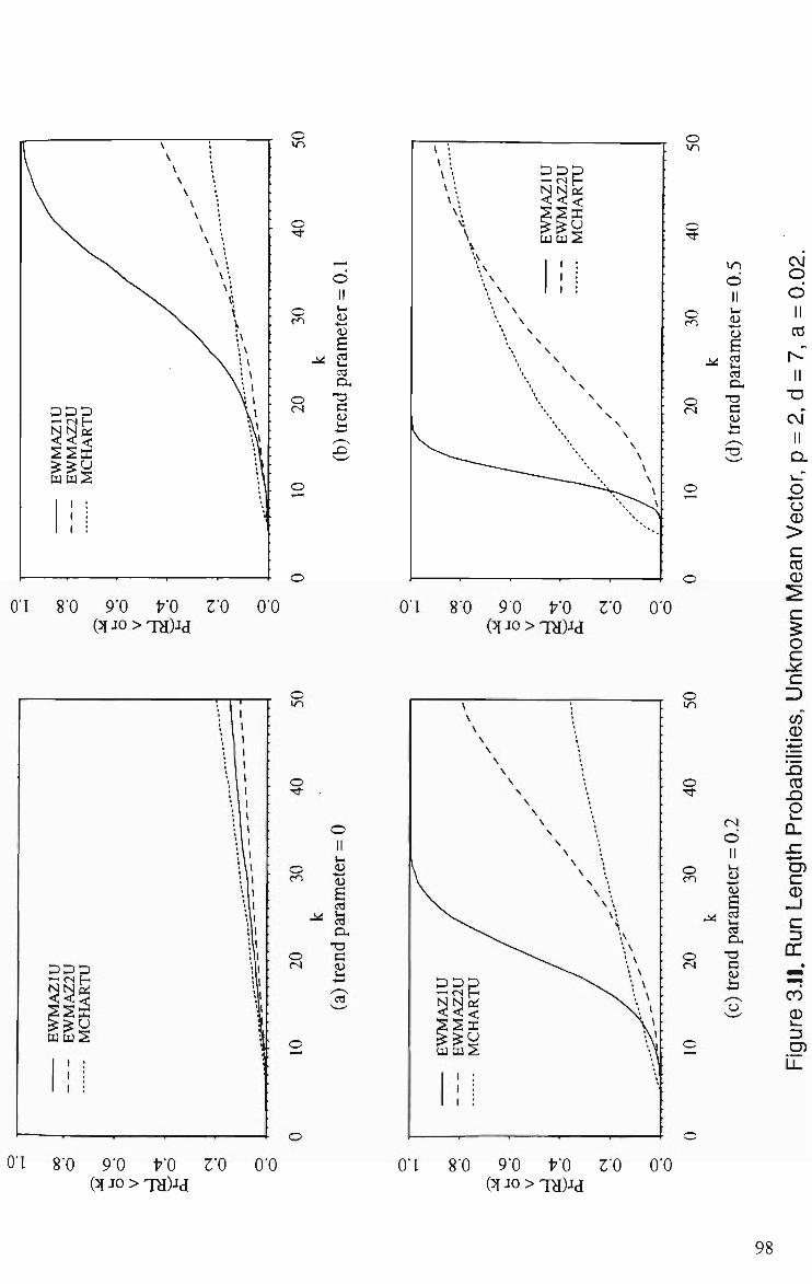
DDp — cs H
^ ^
S S u c 1 : 1 •
1 ;
\ \ • \ \ \ \ \ '. \ ; \ \ \ '. \ '; \'.
" ^ \; ^ \ \1
X i \ V \ u \ \\
•Al
'•}
•X
8'o 9'o t 'o r o (5[J0> 'p l )Jd
o
§
en
O'O
cd O H
o "Q
^ • \ ;
V- -MM \\ ^^1 S S cj
\ WfflS \
•>> . .
•A '. \ \ \
1 ;
I j 1 :
\ \ \ \
s N
\ \
\ \ s
>, \ \
s ">•
V \ \
V "' ^ \ , _ _ ^ '• ^
'—~~-~.^ ""• ^ —'—~-~-..^ "• ^
~" J'> ^ ^v.,,^^ \ •
\N,-' • - .
'**.
1 1 1 1 •
o i n
o Tl-
o en
^
O CS
i n o II
ter
o B
ara
O H
T3 CH (U
O'l 8'o 9'o VO r o (5 iJ0>T^)Jd
O'O
o wn
o T t
o en
U
Q cs
WH (U (U
a cd J3 O H
-a c o «-l
cd
o
o
o en
o cs
CM
o II
t-(
<u
J3 O H
-a c o
'I?
8'0 9'0 VO (51 JO > T ^ J d
ro O'O O'l 8'0 9'o VO ro (51 JO > T ^ J d
O'O
98

EW
MA
ZIU
E
WM
AZ
2U
MC
HA
RT
U
1 ; 1 ; 1 ;
V ; \ •
\ \ V.
\ \
'.\ 1
•A \\ ', \ \ \ \ \ '. \
\ '• ' \ ''' '
V ^
\ 1
A l '.VI
o
o
O'l 8'0 9'0 VO ro (5[=jo>TH)"ad
o en
>!
O CS
o II
•H—>
<u a cd V-i cd O H
-o C
<u
O'O
o
O
o en
O CS
o II
s o B cd
O H
c
I
• \ D D p \ — cs H V N N ei \ < < <
• \ S S K \ ^^H ^ m w S \
\ \
\
1 ; 1 *
\ \
\ '. \
\ \ \
\ \
\ N
\ \
\ \ V '• ^
\ , ^ ^ "'•• ^
^^^~-~.^ '• ^ • ' • . , \
~ ~ ~ ~ ^ « ^ ^
^ ^ ^ " ~ ~ ~ ~ ^ '*
" • • - , . ,
o
o
m o II
en .is
I cd O H
o -a
O'l 8'o 9'0 i7'o r o (5[=jo>'ra)^d
O'O
D D p - ;<s H ^ 1 s s caw2
1 : 1 ; 1 '
• • \ • ; • - • • • - •
\ \ \
\ \ \ \ \ \ \ '. \ • \ •. ^ \ \', \; \ ^ \\ \ \
v ^ ^ \ \ .
^ ^ ^ '• ^ ^ • " - ^ ^ " • ^
^"""^^ I \ ^ \ '• *
\ \ \ \ \
CO
co" II
co"
o
o
o
o rn
O CS
o
CM
o II
- 4 — '
^ O H
-o c is 'o ' ^-^
ean
Vec
nk
now
n M
D
roba
bilit
ies,
CL JC
Len
c 3 DC
e4 • • "
CO CD
Figu
8'0 9'0 VO ro (51 = JO > Tra)Hd
O'O O'l 8'0 9'0 VO ro O'O
99
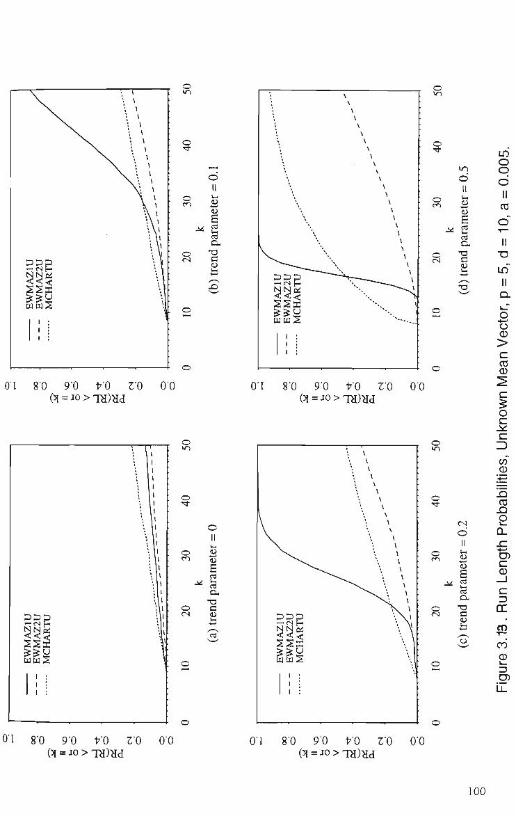
p p p
^ ^ ^ ^Sff i Q EW
M
C
•, \
'. \ • \ • \ ; \ • \ \ \
V • * N. \ \ \ • \
\ \ \ V * \ ( \ '
•A I
'• V \ V
' I
• I
•
O'l 8'0 9'0 VO ro (5i = J0>TH)Hd
DDp — cv) H
o m
o
o en
O CS
cd
cd O H
-a c
', \ *, \ \ ' *, ', \ \ \ \
\ \ '\
'\
D D p ^^%
lis 1 '
1 ;
\ \ \ \ \ \ \ \ \ \ \ \ \ \ \ \ \ \ \ \ \ V \
• — - - ~ _ \ _ \ '.
"' ^~~~~~~~-~- \ ^ ^ ^ • ^ o •
1-• " . . .
- T ' 1 1 •
o
o •5t
o en
J^
O CS
un o II
B cd
O H
TD C WH
005.
d II
CO
o
II • D
LO
O'O O'l 8'0 9'o t 'o ro (5[ = J0>TH)^d
O'O
I
I
o i n
o
(-) en
o cs
J4
0)
amet
dp
ar
o p
cd
--cs H ^ ^ ^ S S K
iu D
1 :
1 •
1 :
— 1 — *
\ \ \ \ \ \ \ \ \ \ \ \ \ \
\ ^"-•^ \ ^
^ ^ \ \ \ \ i V
\ \ 1
\ I V I
\
o m
o
CM
d 11
4>
<y cd
Jd O H
O CS
T3 C
o CD
>
c CO CD
c o c c CO CD
CO
O
C
CC
CO
CO
CD
O'l 8'0 9'o VO ro (5[ = J 0 > T ^ ) ^ d
O'O O'l 80 90 VO ro (5{=J0>'Pi)^d
O'O
100
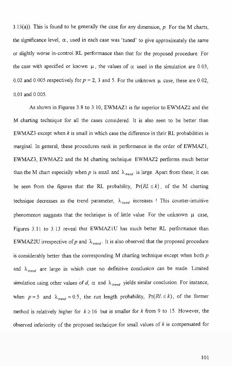
3.13(a)). This is found to be generally the case for any dimension, p. For the M charts,
the significance level, a , used in each case was 'tuned' to give approximately the same
or slightly worse in-control RL performance than that for the proposed procedure. For
the case with specified or known p , the values of a used in the simulation are 0.03,
0.02 and 0.005 respectively for;? = 2, 3 and 5. For the unknown p case, these are 0.02,
0.01 and 0.005.
As shown in Figures 3.8 to 3.10, EWMAZl is far superior to EWMAZ2 and the
M charting technique for all the cases considered. It is also seen to be better than
EWMAZ3 except when k is small in which case the difference in their RL probabilities is
marginal. In general, these procedures rank in performance in the order of EWMAZl,
EWMAZ3, EWMAZ2 and the M charting technique. EWMAZ2 performs much better
than the M chart especially when/? is small and A, g„ is large. Apart fi-om these, it can
be seen fi-om the figures that the RL probability, ^x{RL <k), of the M charting
technique decreases as the trend parameter, A-, g„ increases ! This counter-intuitive
phenomenon suggests that the technique is of littie value. For the unknown p case.
Figures 3.11 to 3.13 reveal that EWMAZIU has much better RL performance than
EWMAZ2U irrespective ofp and X, g„ . It is also observed that the proposed procedure
is considerably better than the corresponding M charting technique except when both p
and X,^g„d ^re large in which case no definitive conclusion can be made. Limited
simulation using other values ofd, a and A, g„ yields simUar conclusion. For instance,
when p=5 and X^^„d=0.5, the run length probability, FT(RL<k), of the former
method is relatively higher for A: > 16 but is smaUer for k from 9 to 15. However, the
observed inferiority of the proposed technique for small values of k is compensated for
101

by its lower likelihood of false alarms. Another interesting point that can be noticed from
the figures is that the RL probabUities for the M chart are higher for the unknown p case
than for the known p case. Thus, if process changes are anticipated to be in the form of
linear trends and an M chart is to be used, U is advisable to use that which does not
assume known value of p even though p is specified or known.
In the comparison above, U is assumed that the trends occur immediately after the
process set-up. This is, however, not always the case in practice. For deferred trends, the
EWMA procedures : EWMAZl, EWMAZ2, EWMAZ3, EWMAZIU and EWMAZ2U
can be expected to improve in performance since the sample covariance estimate used
with each is based on some in-control observations and has greater degrees of fi"eedom.
However, it is readily seen that this deferral of trends has no effect on the RL properties
of the M charting techniques. Thus, h appears that the proposed procedures outperform
the M charting techiuques for most circumstances.
The results for step shiflis are shown in Figures 3.14 to 3.19 for various
combinations ofp, r and X . As shown in Figures 3.14 to 3.16, EWMAZl is far superior
to EWMAZ2 and is as good as or significantly better than EWMAZ3. For r = 10 and
X = 2 or 3, the RL probabilities of EWMAZl wUhin short runs are slightly lower than
those for the other two procedures. For the case with unknown parameters, it is evident
from Figures 3.17 to 3.19 that EWMAZIU is more likely to 'pick up' the shift
irrespective ofp, r and X .
Although Zl^, Z\ and similarly transformed variables as given by (3.5), (3.6)
and (3.13) can be used in their own rights, some limited simulations not reported here
indicate that using the associated EWMA procedures resuUs in significantly better RL
performance for step shift and linear trend condUions. However, control charts based on
102

statistics (3.5) and (3.6) are good as the fiUers to isolate outUers and they wUl exhibU
various discernible point patterns for other erroneous processes. Thus, it is
recommended that in practice these charts be used and supplemented by EWMAZl and
EWMAZIU respectively.
Note that, EWMAZl and EWMAZIU are also sensUive to other process
disturbances including changes in the variance-covariance structure of the measured
variables. To distinguish between location and scale changes, a reasonable approach is to
construct maximum likelihood ratio or Schwarz information criterion (SIC) statistics for
the respective out-of-control models (see Chen and Gupta (1994, 1995)) and use the p-
value as an indicator of the most probable type of change. This is an interesting problem
which needs fiirther investigation and U wiU not be considered fiirther here.
3.7 Computational Requirements
In this work, evaluation of the standard normal distribution. Us inverse, chi-
square and F distribution flinctions are required in order to compute the trasformed Z
statistics. In addition, computation of the argument statistics 7 's involve matrix
muUiplication and inversion. To implement the proposed control scheme, therefore,
requires some fairly complex algorithms. Fortunately, these are widely avaUable and have
been built into most of the commercial statistical software packages. The simulated data
and the charts in this and the next chapter were generated and made by the authour using
programs written in S-plus.
103

—«cs m
UJ m U
O'l 9'0 l 'O (5f = JO > TH)JH
9-0 VO (5f = 10 > 1>T)JJ
9-0 VO (2f = JO > 'T>T)-icT
9'0 t 'O (5t = JO > 'T>i)j^
90 t-'O (51 = JO > TH)Jc^
O'l 8'0 9'0 170 (51 = JO > TH)Ja
to
c
O
en il s i 2
<^ 13 UH
«s 2
o «s
II
Q-O -
EW
MA
Zl
EW
MA
Z2
- E
WM
AZ
3
: ' 1
\ \ \
\ \ !
\ \ \ ;
\ \ \
\ •
o
O
t3 CD
>
c CO CD
(/}
(J) Q. 05
CO
(fi
CD CO
O
C CD
_J C
CC
il ^
o CO
CD i _
D
o c
Q o <N
o cs
: o
O
O'O
104

O'l 8'0 9'0 t-'O (5r = JO > 7>T)-iJ
TO O'O O'l 8'0 9'0 t-'O (5( = JO > TH)JH
O'l 8'0 9'0 l 'O (5f = JO > 'T>T)jj
O'l 9'0 VO (5f = JO > TH)JtT
— es m
t x iuu
O'l 8'0 9-0 l 'O (5( = JO > TH)J,T
--H cs en
^ ^ ^ S S ^ ^^1 cu ta u
1 1 ! 1
\ \ \
\ \ '• i \ \ i :
\ \ ' . •
\ \ '. \ \ ;
\ \ '•,
\ \ '. '. \ \ \ V \
\ '
V \ ' ,
V
\ •
o in
c
^ .5 ^ 13
o c o o •- c
o' cs II
o
II
CO
CO Q . CD
C/D
CO CD
X3 CO
JD O _
Q_
C CD
_ l
C Z3
DC
cd
13 D5
LL
O'l 8'0 9'0 VO (5f = JO > TH)-icT
ro O'O
105

O'l 8-0 9'0 t'O (51 = JO > q>i)Jj
90 1 0 (51 = JO > Tii)iS
106
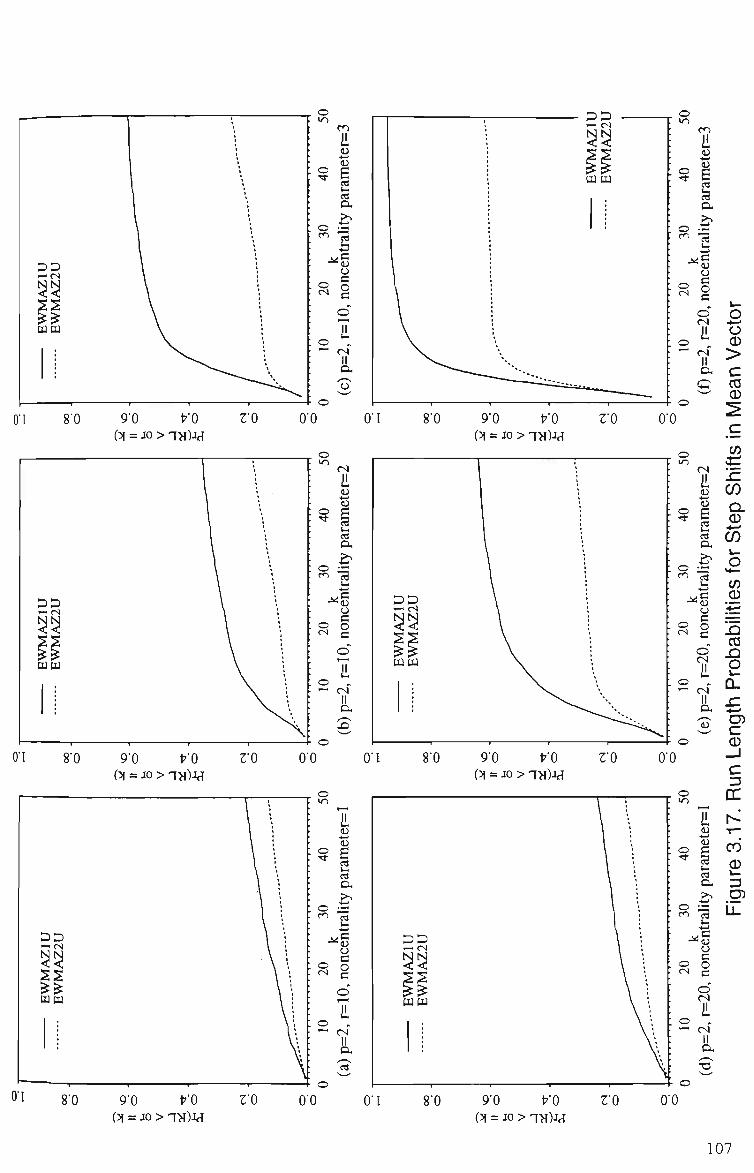
9'0 t 'O (5f = JO > T>i ) ja
9'0 t 'O (5f = JO > -[•H)jj
o in
o
o en
cs il (1) . t - i iJ
B I , c<3 O -
ality
h
o cs
o
o c o
r=20
cs'
^ CO (^ CD * -C/J
for
(/; CD —•
J3 CO
rob
CL
o
O'l S'O 9'0 VO (31 = JO > q>r)JcT
9'0 VO (5f = JO > TH)JcT
O'O
U U
80 9'0 l 'O (5f = JO > T>T)Ja
9'0 t'O (5f = JO > i>T)J<T
107
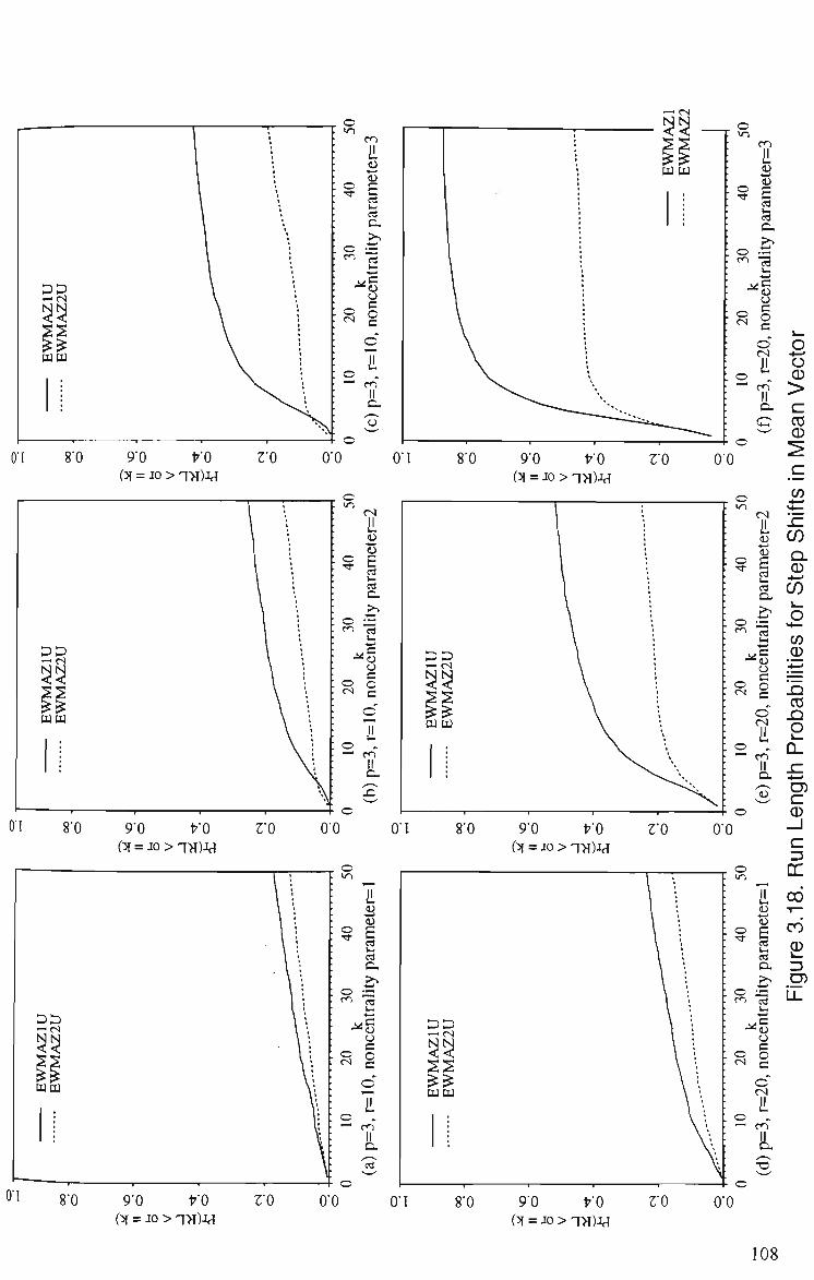
^ o . m en
II \ - i
a * j
(U • ^ § cd
13 c
: o . ^ • ^ 13
b< <->
o
20
non
. o cs
o ' l ^ en
II D-
CT
u. O *-> o CD
>
c CO CD
9-0 l 'O (5f = JO > l>T)JcT
9-0 t 'O (5f = JO > T>T)JcT
00
S'O 9-0 t 'O (5f = JO > TH)JcT
ro O'O O'l 8'0 9'0 VO (5f = JO > TH)-i<T
ro 00
uu
80 9'0 l 'O (51 = JO > q>T)Ja
O'l 80 9'0 fO (5( = JO > TH)JcT
ro 00
108
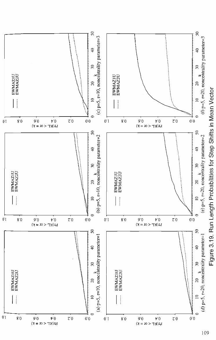
O'l 8'0 9'0 VO (5f = JO > TH)JcT
9'0 t 'O (5f = JO > q>T)j^
9'0 t 'O (5f = JO > 1>T)J^
9'0 t 'O (:!f = JO > 'T-H)JcT
—'CS
U U
01 8'0 9-0 l 'O (31 = JO > T^ilJcT
9'0 l 'O (51 = JO > 1>I)JH
109
CHAPTER 4
DISPERSION CONTROL FOR MULTIVARIATE
NORMAL PROCESSES ^
4.1 Introduction
Over the last decade, the problem of muhivariate quality control has received
considerable attention in the literature (see for eg., WoodaU and Ncube (1985), Murphy
(1987), Healy (1987), Crosier (1988), PignatieUo et al.(1990), Doganaksoy et al.(1991),
Sparks (1992), Tracy et al.(1992), Lowry et al.(1992), Hawkins (1991,1993), Hayter et
al.(1994), Chan et al.(1994) and Mason, Tracy and Young (1995)). This work has
focussed on the detection of parameter changes, departures from distributional
assumptions, and the identification of out-of-control variables. Most of the work is based
on the assumption that the observation vectors, X/5 are independently and idenrically
distributed (i.i.d) multivariate normal variables and that the true values of the process
parameters, in particular the process variance-covariance matrix, Z , are known. In
chapter 3, a control procedure for monitoring the mean level of muhivariate normal
processes for situations where prior information about the in-control process parameters
is unavailable has been presented. It was demonstrated that the procedure is particularly
usefiil when subgroup data are used.
Whilst substantial work has been devoted to the control of the process mean
vector, p , very little emphasis has been placed on the importance of monitoring and
controlling Z . In fact, the issue is a formidable one due to the complexity of the
This chapter is based on the papers entitled 'Dispersion Control for Multivariate Processes', Australian Journal of Statistics 38 (3), pp.235-251, 1996 and 'Dispersion Control for Multivariate Processes - Some Comparisons', Australian Journal of Statistics 38 (3), pp.253-273, 1996.
110
distribution theory involved. One exception is the paper by Alt et al.(1986) who
proposed two control techniques for S ; one based on the UkeUhood ratio principle and
the other that makes use of the sample generalized variance, which is sometimes taken as
a measure of dispersion or spread of muhivariate processes. Although tradUional
muhivariate control charts such as the Hotelling x^ or T^ charts may signal certain
shifts in S (see Hawkins (1991)), other particular changes in Z wiU remain undetected.
This is also true for the technique based on generaUzed variance. For instance, if H
shifts in such a way that the resuhing process region (i.e the ellipsoidal region in which
almost all observations fall) is contained completely wUhin the undisturbed one, this
'shrunken' process is unlikely to be detected by a x^ chart, especially when the sample
size is smaU. In addition, Hawkins (1991) stated that 'measures based on quadratic forms
(like T ) also confound mean shifts with variance shifts and require quUe extensive
analysis following a signal to determine the nature of the shift'. Note that the ' T^' term
that he used actually refers to the more commonly caUed ^^ statistic which uses
(presumably) the true value of the process covariance matrix. When 'special' or
'assignable' causes affecting both process parameters are present, it is also possible that
the effect of the mean (vector) shift is masked or 'diluted' by the accompanying change
in the variance-covariance matrix.
The purpose of this chapter is to present some control procedures for the
dispersion of multivariate normal processes based on subgroup data. Special attention is
drawn to the situations where prior information about S is not available as is often the
case in situations of short production runs, which have become increasingly prevalent.
When Z is specified or assumed known, the proposed procedure involves the
111
decomposition of the sample covariance matrix and uses the resulting independent
components, which have meaningfial interpretations, as the bases for checking the
constancy of the process covariance matrix. Another possible approach is also outUned
for this case. As for the case where E is unknown in advance of production, the
proposed procedure is adapted from the step-down test of Anderson (1984, p.417)
which is based on the decomposition of the UkeUhood ratio statistic for testing the
equality of several covariance matrices. When these procedures are used together wUh
Hotelling x^ or T -type charts, they supplement the latter by providing independent
information about the stability of the process covariance matrix. Furthermore, these
techniques effectively replace existing procedures to provide enhanced detection of
general shifts in H .
This chapter is organized into five subsequent sections. In 4.2, the underlying
methodology is presented. In 4.3, appropriate control statistics are given for both the
cases regarding prior knowledge or lack of prior knowledge of the process covariance
matrix. Methods to cope with rank deficient problem which arises from the use of sample
sizes not exceeding the number of quality variables are briefly considered in section 4.4.
Comparisons are made between the proposed techniques and various competing
procedures in section 4.5. In 4.6, an Ulustrative example is presented. In the last section,
the effect of incorporating independent components from the decomposition to form an
aggregate-type statistic, on the control performance, is examined for the known E case.
The total discourse is given in the context of the manufacture of discrete Uems.
4.2 Methodology
Suppose that the vectors of observations on p correlated product characteristics,
X/s follow a multivariate normal A^^(p,S) distribution with mean vector p and
112
covariance matrix S when the process is operating under stable condUions. In practice,
the validity of this assumption should be checked using, for example, a muhivariate
normal goodness-of-fit test (Gnanadesikan (1977)). The aim here is to develop control
procedures for monitoring and controUing the dispersion of such a multivariate process
based on rational subgroups where the sample size, n may vary. It is assumed in this and
the next section that n> p so that the suggestion works. When this is not the case, Uttle
adaptation of the proposed procedures as discussed in section 4.4 is required.
In order to provide more flexibility, ease of implementation and better control of
the false alarm rate than existing procedures, as well as to facilitate the interpretation of
out-of-control signals, it is suggested that the sample variance-covariance matrix be
partitioned into various statistically independent components having physical
interpretation and known distributions. These components are then used to indicate the
stability of the process covariance matrix.
It is well known, that under the stable or in-control normality assumption, the
sample covariance matrix, S, multiplied by the factor ( « - l ) foUows the Wishart
distribution with parameters [n -1) and Z , denoted by
in-l)S~Wp(n-l,I)
Let the sample and population covariance matrices be similarly expressed in partitioned
form as foUows :-
S = rs 11
V»21
^12
>22>
^Sl i S
Sj2 ; S
12
22 Z = S.. \ E,.
11
V Ezi i I 22 ^
r_2
1:12 '22
where Sl {(^l), Sjj ( E n ) and Sjj (Z22) denote respectively the sample (population)
variance of the 1st variable, the vector of sample (population) covariances between the
113

1st and each of the remammg variables, and the sample (population) covariance matrix
excluding the 1st variable. Next, define
^22.1 = ^22 - ^21^11 S j 2
^12 ^12
then according to a weU-known theorem (see for eg., theorem 6.4.1, p. 120, Giri (1977),
where Z(22)-X(2i)S^ii)S(i2) in (c) should be replaced by Z(ii)-Z(i2)S^)Z(2i)
using his notation),
(i) S22,1 ^^ independent of S^,Si2 V ~ y
(ii)(«-lK~a?xli,
(iii) {n -1)822.1 ~ Wp-i(n - 2,Z22.i) where Z22.1 = Z22 "^21 ^il ^u
E12 E12 '22
s 12 2 „2
^l
^v _ ^ (iv) The conditional distribution of - ^ , given S^ = j , is A'
5'i
E 12 ^ 2 2 « l
^Oj '(«-l)5?^
Note that 822,1 and S22.1 ^ ^ e denote respectively the conditional sample and
population covariance matrices of the last (p-l) variables given the 1st. Note also that
S12 2! 12 ~ and - ^ represent respectively the vectors of sample and population regression S^ aj
coefficients when each of the last (p-l) variables is regressed on the 1st variable.
114

• 12
Furthermore, S^ , -^ and S22.1 may be regarded as independent components following
the above decomposition of the sample covariance matrix 8. Further, decomposing
822,1 in the same manner yields ^2,1 (the condUional sample variance of the 2nd
Sl2.1 variable given the 1st one), —— (the vector of regression coefficients when each of the
last {p - 2) variables is regressed on the 2nd whilst the 1 st variable is held fixed) and
834 ^^. 12 (the conditional sample covariance matrix of the last (/?- 2) variables given
the first two) which are independently distributed as
<:2 -(A E>2\r.2 0 j l P l l & . v 2
^12.1 / e 2 _ „ 2 _ A ^
„2 / ^2.1 -•^2.1 ^V ' 2»1
(«-l)
•^12.1 y
^-^ -^3,. . . ,p. 1,2
C72.1 ' ( « - 1 ) 5 2 . 1
and S3,...,;.l,2 ~ - ^ ^ p - 2 ( « - 3 , i : 3 , . . . , p . u ) ,
where R^2 and Pjj are respectively the squares of the sample and population
correlations between the 1 st and the 2nd variables. Repeating the above procedures until
fiirther decomposUion is impossible resuUs in p scaled chi-square variables S^ ,
Sj,i j _ ^ , j-2,...,p and p-l conditional (univariate or multivariate) normal
variables which are independent and have meaningfiil interpretations. 5^.1 ^_i here
denotes the condirional sample variance of theyth variable given the first7-1 variables.
Note that the ordering of the variables is not unique. In fact, there are/?! possible
permutations each of which resuUs in (2/?-l) terms in the decomposition. If aU of these
115
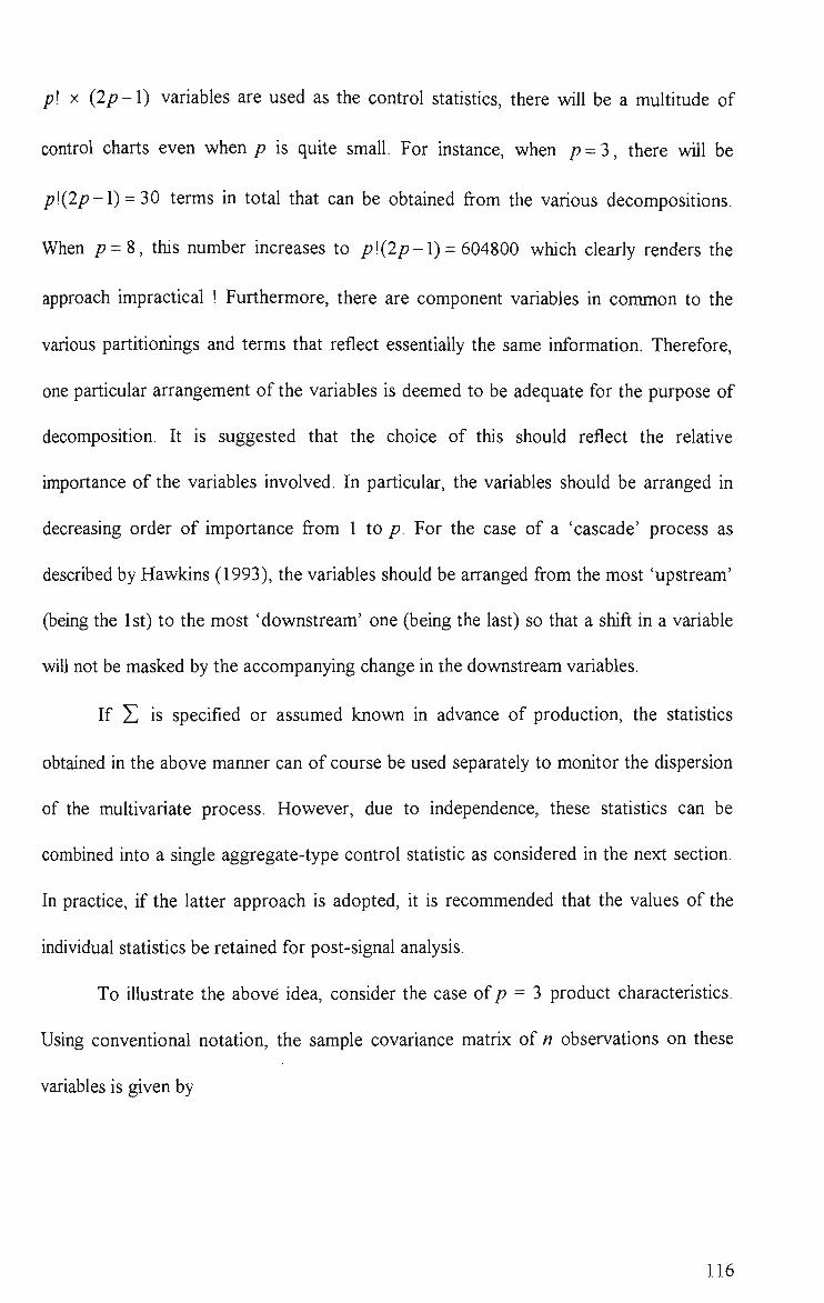
p\ X (2/7-1) variables are used as the control statistics, there wiU be a multitude of
control charts even when p is qmte small. For instance, when /? = 3, there wUl be
p\{2p-l) = 30 terms in total that can be obtained from the various decompositions.
When /7=8, this number increases to /7!(2/7-l) = 604800 which clearly renders the
approach impractical ! Furthermore, there are component variables in common to the
various partUionings and terms that reflect essentially the same information. Therefore,
one particular arrangement of the variables is deemed to be adequate for the purpose of
decomposUion. It is suggested that the choice of this should reflect the relative
importance of the variables involved. In particular, the variables should be arranged in
decreasing order of importance from I to p. For the case of a 'cascade' process as
described by Hawkins (1993), the variables should be arranged from the most 'upstream'
(being the 1st) to the most 'downstream' one (being the last) so that a shift in a variable
will not be masked by the accompanying change in the downstream variables.
If YJ is specified or assumed known in advance of production, the statistics
obtained in the above manner can of course be used separately to monitor the dispersion
of the multivariate process. However, due to independence, these statistics can be
combined into a single aggregate-type control statistic as considered in the next section.
In practice, if the latter approach is adopted, U is recommended that the values of the
individual statistics be retained for post-signal analysis.
To illustrate the above idea, consider the case of/> = 3 product characterisfics.
Using conventional notation, the sample covariance matrix of n observations on these
variables is given by
116
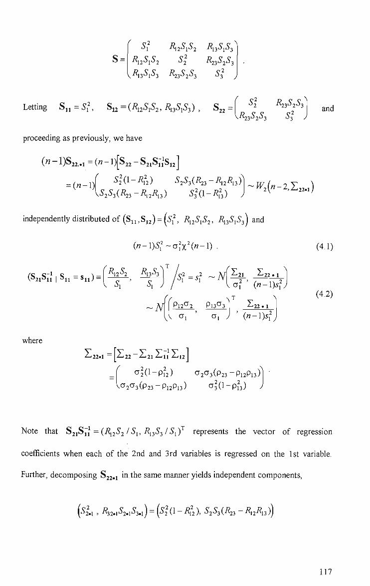
s= ^l •^2'^1'^2 -^IS'^l'^S
O2 -f^3'J2'^3 R12S1S2
^•^B'^l'^S ^3^ 2^ 3 '3 y
Letting Sii = ^ ^ 81^ =(i?i2'^i52, i^,3' i^3) , 822 =
proceeding as previously, we have
( « - l ) S 2 2 . . 1 - ( « - l ) [ S 2 2 - S 2 i S i X ]
*-*2 'f\23'J2'^3
V./V23O2O3 03 y
= ( « - ! ) ^2 (1 - -^12 ) ' ^ 2 ' ^ 3 ( ^ 3 " -^12-^13 )
^ 2 ^ 3 ( ^ 3 - ^ 1 2 ^ 1 3 ) " ^ ' ( l - ^ n ) J
and
f^2(«-2,I ,2. l )
independently distributed of (811,812) = (5'l^ i?i2^i^2' RuS^S^) and
(n-l)S^-oh'(n-l)
^-1 (821811 Sii - S i i ) Rl2^2 ^\3^3
V Si s, J 's^=s^ -N ^ 2 1 ^ 2 2 » i
^ a f ' (n-l)s^J
Pn^2 P l3^3^
V a, ^1 J
^ 2 2 «i
(«-l)^?
(4.1)
(4.2)
where
'^22.1 - [-^22 -^21 -^11 -^12 I
«72(1-Pl2) CJ2CJ3(P23-P12PI3)
^2^3(P23-P l2P l3 ) f^3(l-p?3) J
Note that SjiSi/=(^^12^2/-^i'-^13*^3/"^i)^ represents the vector of regression
coefficients when each of the 2nd and 3rd variables is regressed on the 1st variable.
Further, decomposing S22.1 in the same manner yields independent components,
(' '2.1 , A2.1'^2.1'^3.1 j = ( 2 (1 - -^12)' 'S'2^3(i^3 - ^12^13)]
117
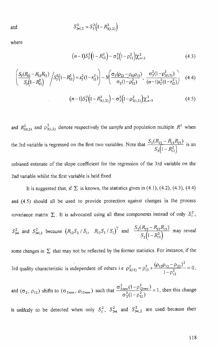
and ^3,1,2 - -^3^1 - ^3(1,2))
where
(«-l)^2'(l-A'2)~a^(l-pf2)x'-2 (4.3)
^ ^ ^ / ^ ^ ( l - i ? 2 ) - 2 ^ ( 1 - 4 ) <^3 (P23 - P12P13 ) ^ 3 (1 - P3(U))
• ^ (4.4) 1, a2(l-p^2) («-l>52(l- ' i2);
(n - l)S^{l - 4 ,2 ) ) ~ CT?(l - P3(U))X13 (4.5)
and RL 2) and P3(j 2) denote respectively the sample and population multiple R^ when
the 3rd variable is regressed on the first two variables. Note that ——-^1 T T ^ ^ is an
unbiased estimate of the slope coefficient for the regression of the 3rd variable on the
2nd variable whilst the first variable is held fixed.
It is suggested that, if E is known, the stafistics given in (4.1), (4.2), (4.3), (4.4)
and (4.5) should aU be used to provide protection against changes in the process
covariance matrix E • It is advocated using aU these components instead of only S^ ,
r ' / - n _ D D \
2 1 and 3 .12 because (RuSifSi, R^S^ f S^) and - ^ ^ ^j^ may reveal •^2(1-^12]
some changes in E that may not be reflected by the former statistics. For instance, if the
3rd quality characteristic is independent of others i.e P3(i2) = P13 + 2 ~ '
and (02, P12) shifts to (G2„^, Pnne.) such that ^^J^^-P^^"^^ = 1, then this change <^2(1-Pl2)
IS unlikely to be detected when only 5"! , 82,1 and '3 ,12 are used because their
118

respective distributions are not distorted under these circumstances. However, this
change induces a shift in the slope coefficient for the regression of the 2nd quality
characteristic on the first. Therefore, it is possible to 'pick up' such a change if the vector
of population regression coefficients (p^cJi/^b Pn'^s/'^i) is also monitored based
on the corresponding vector of sample regression coefficients {R12S2 IS^, R12S3 / S^)
which is known to be bivariate normal for fixed S^ under the in-control and normality
assumption (see (4.2)). If the traditional HoteUing X^ chart based on these coefficient
vectors is used, it is readily seen that its statistical performance depends on the
noncentrality parameter
(«-l)^?(±Va^^ -CT (1-P?2) -Pi2^2) 2~2 2
Cia2 ( l -p i2 )
where the +ve sign is used when Pi2new > and the -ve sign otherwise. Thus, whilst the
use of the control statistics S^ , S2,i and iS'3 .12 are unlikely to register the change, it is
clear that the probability of detection by the Hotelling ^^ chart may increase depending
on the value of S^ for the current subgroup, the sample size, n, as weU as the dispersion
parameters. The same is true if the aggregate-type control statistic as given in the next
section is used.
As an alternative, the foUowing method of decomposition may be employed. Let
S^j^ and I]<y> be the upper left-hand square submatrices of S and S respectively, of order j . Also, let Sr 1 and 2r,i denote respectively the sample and population
119
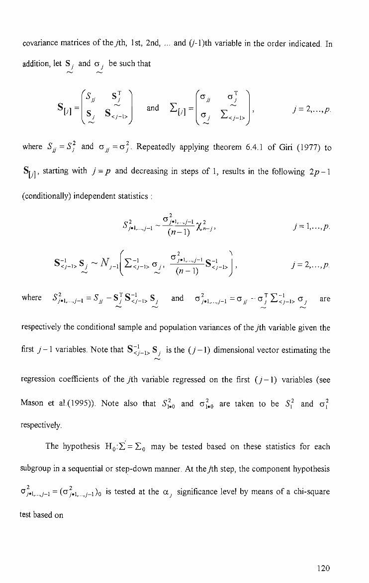
covariance matrices of theyth, 1st, 2nd, ... and (/'-l)th variable in the order indicated. In
addition, let Sy and a j be such that
%] -V ~ y
and Zf.j =
.T A ;;
^ i ^<j-i> 7 = 2,...,/?.
where S^^ =Sj and Ojj =GJ. Repeatedly applying theorem 6.4.1 of GUi (1977) to
8r 1, starting with j = p and decreasing in steps of 1, resuUs in the foUowing 2p-l
(condUionally) independent statistics :
r,2 '^yi,...,;-!
^y«l,...,;-l 2
(n-l) ^''-^' 7 = 1,...,/?.
'<;-i> ^y 8, ~A^;_i z;;_i>ay. a /•1,...,;-1 c _ i
(«-l) s;; '-1> 7=2,...,/?.
^^^'•6 ' ' .i y_i = Sjj - S j S;;._i, S . and o%,_j_, = a^. - a J !.-]_,, Oj are
respectively the conditional sample and population variances of theyth variable given the
first j-l variables. Note that S~J_i> 8^ is the ( / - l ) dimensional vector estimating the
regression coefficients of the y'th variable regressed on the first (/' -1) variables (see
Mason et al.(1995)). Note also that S^Q and of.o are taken to be S^ and af
respectively.
The hypothesis Ho:E = Eo niay be tested based on these statistics for each
subgroup in a sequential or step-down manner. At theyth step, the component hypothesis
2 2
cjy.i y_i = (Oj,i_j_i)o is tested at the a^ significance level by means of a chi-square
test based on
120

7 # ^ • ( '
(cfy.i,..,/-i)o
If there is failure to reject this sub-hypothesis, then a^ = cSj\ (or
S<J_i> cr = | S<y_i> j ^ C7y ) is tested at significance level bj on the assumption that '~ V '~y Q
E<y_i> = (E<y_i>) . The test statistic.
^ ~ ^ ~ ^ 0 y ^^/.l,...,y-ljg V ~ v ~ . (4.7)
is a Xy-i variable if the component hypothesis is true. If there is failure to reject this
component hypothesis, then the (/+l)th step is taken. The hypothesis Ho:E = Eo is
accepted provided there is failure to reject all the 2/?-l component hypotheses. The
overall significance level of this test for each subgroup is then given by
i-na-^;)n(i-5;). 7=1 7=2
Anderson (1984, p.417-418) has presented such an approach for testing the
equality of covariance matrices as an alternative to the standard maximum UkeUhood
ratio procedure, with the unknown parameters replaced by appropriate estimates based
on previous subgroups and other suitable adjustments made. The resulting statistics for
all successive subgroups follow Snedecor-F distributions and were shown by this author
to be stochastically independent (Anderson (1984), theorem 10.4.2, p.414). Although
this method is not proposed in the context of SPC, it can be used for monUoring the
stability of the process covariance matrix for which the true in-control value is unknown
and cannot be reliably estimated. FoUowing the conventional approach, however, a
121
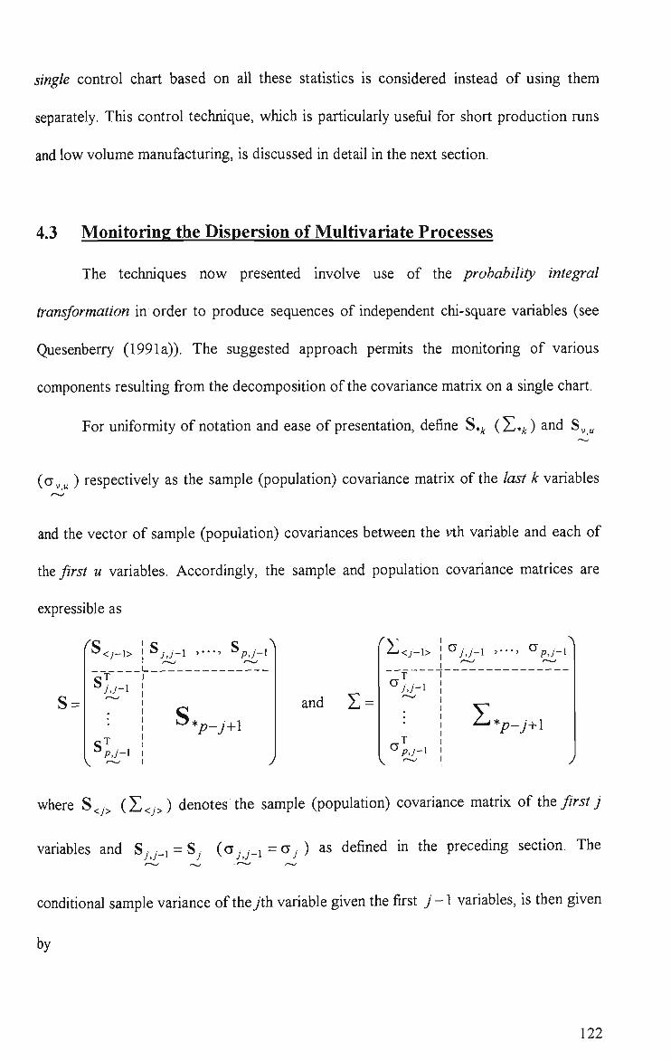
single control chart based on all these statistics is considered instead of using them
separately. This control technique, which is particularly usefiil for short production runs
and low volume manufacturing, is discussed in detaU in the next section.
4.3 Monitoring the Dispersion of Multivariate Processes
The techniques now presented involve use of the probability integral
transformation in order to produce sequences of independent chi-square variables (see
Quesenberry (1991a)). The suggested approach permits the monitoring of various
components resulting from the decomposition of the covariance matrix on a single chart.
For uniformity of notation and ease of presentation, define 8* iY*k) and 8^^
(ay„) respectively as the sample (population) covariance matrix of the last k variables
and the vector of sample (population) covariances between the vth variable and each of
thQ first u variables. Accordingly, the sample and population covariance matrices are
expressible as
(^<j-\> I S y j - l ,••
8 =
s ^
fj-i I
gT j V-7+1
^y ^<j-i>
and S = 'jj-i
^pj'i
^jj-i ' • • • ' ^pj-i
^-^ *p-j+i
where 8<.> (Z<,>) denotes the sample (population) covariance matrix of the first j
variables and Sy y_i = 8y (ayy_i=CTy) as defined in the preceding section. The
conditional sample variance of theyth variable given the first j - 1 variables, is then given
by
122
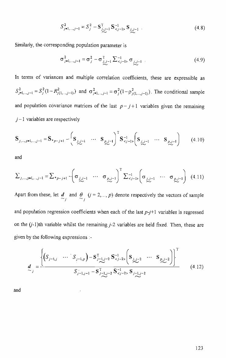
; .1 , . . . , ; -1 - ^j - ^jj-l ^<j-l> » y , y - i • (4.8)
SimUarly, the corresponding population parameter is
^;.l,...J-l = Crj - a j_y_l Z;j-1> CTy y_i (4.9)
In terms of variances and muhiple correlation coefficients, these are expressible as
' y.i,...,;-i ='^;(l~^y(i,..j-i)) and <^;.i,...j-i = cyy(l-py(i y_i)). The conditional sample
and population covariance matrices of the last p-j + l variables given the remaining
j - 1 variables are respectively
^j,...,p>\,...j-\-^*p-j+\ ^j,]-i '" ^pj-i o - l >'</-l> V.y-1 - S,,y_i (4.10)
and
^ ; , . . . , p . 1,...J-1 - ^ * p-j+i y j - i ' p j - i y~^
'jj-i p j - i (4.11)
Apart from these, let d and ^ (/ = 2,..., /?) denote respectively the vectors of sample
and population regression coefficients when each of the last p-j+l variables is regressed
on the (j-l)th variable whilst the remainingy'-2 variables are held fixed. Then, these are
given by the following expressions :-
\\^J-hj '" ^j-l,p)~^j-hJ-2^ <j-2> 'j,J-2
d =
and
^J-lJ-l ^j-lJ-2 S<y-2> Sy_l,y_
M P j - 2
(4.12)
123

e =
(ay_i,y - Oy_,^)-aJ_i^y_2l;;._ -2> ^ ^ ; . ; - 2 - Op^j_2
(4.13) ^ /-1,/-1 Cy y_l y_2 Z <y_2> a y_l y_2
Note that d and 0 should be interpreted as the vectors of uncondUional sample and ~ 2 ~ 2 ^
population regression coefficients when each of the last p-l variables is regressed on the
1st variable and these are given by
d J'" ••• ''^y and e = K ^ l J ~ 2 5jj ~ 2 a n
respectively.
In addition to the above, the following notation will be used :-
<!>"(•) : inverse of the standard normal distribution fiinction
X V (•) '• distribution fiinction of a chi-square variable with v degrees of freedom
^vi;v2 (•) • distribution fiinction of an F variable with vl numerator and v2
denominator degrees of freedom
In the following subsections, control statistics for monitoring the stability of the
process covariance matrix are presented for the case where eUher E is known or
unknown. In order to specify the chronological order of the subgroups, the sample
statistics are indexed with an additional subscript enclosed wUhin a bracket.
Case (D : E known
In practice, the process parameters, in particular the true value of the process
covariance matrix E , is never known exactly. Instead, U is estimated based on a
124
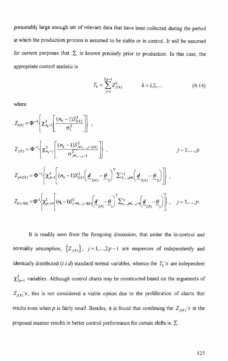
presumably large enough set of relevant data that have been collected during the period
in which the production process is assumed to be stable or in control. It will be assumed
for curtent purposes that E is known precisely prior to production. In this case, the
appropriate control statistic is
n 2p-l
2 J(k) k = l,2,. (4.14)
where
Zm = ^~'< KiriK-l ( « . - ! ) % )
.2 O,
^m = ^~' (j^k ^)^ j.\,...J-\{k)
•/•i , . . , ;-i
j-2,...,p.
'P+Kk) = 0 -1 Xp-1 (^.-D'^iw
\~2(k} 0 I.-2'i d -e
\^2{k)
^p^j-m-^ • ILp-j-w («^-l>S^_H..,y. •m
( d -
V.~;(fe)
A
-e ~;V
E- '/,..,M-.j-i d -6 V~;(fc) ~ ;y
, 7 = 3,...,/?.
It is readily seen from the foregoing discussion, that under the in-control and
normality assumption, IZy^j^J, j = l,...,2p-l are sequences of independently and
identically distributed (i.i.d) standard normal variables, whence the T/^'s are independent
Xip-i variables. Although control charts may be constructed based on the arguments of
Zj(^k^'s, this is not considered a viable option due to the proliferation of charts that
resuUs even when/? is fairly small. Besides, U is found that combining the Zj^i^^'s in the
proposed marmer results in better control performance for certain shifts in E .
125

Note that since the arguments of the normalizing transformation are independent
chi-square variables, a single aggregate-type control statistic may be obtained by
summing them. The resuhing test is commonly called the sum test. Similarly, the sum
may be taken over the transformed statistics Zj^^^s giving a sequence of independent
N{0, 2p-l) variables. In either case, however, certain deviations of the process
covariance matrix from the specified E are likely to be missed by the resuhing
techniques. In particular, if E shifts in such a way that the values of some Zj^^^^'s tend
to be larger whilst others tend to be smaller than that attributable to common causes,
then this type of change is unlikely to be detected by the resuhing charts. To provide
protection against such changes, U is suggested that the Zy ^ ' be squared before
summation as in formula (4.14), and only an upper control Umit is then necessary. It
should be noted that a similar techiuque can also be developed based on the alternative
partitioning method outlined in the foregoing section. This is, however, not considered
fiirther because it is found that the proposed technique always performs better.
Case (n) : E unknown
In the absence of prior information about the process parameters, a natural
solution is to estimate the various components resulting from the decomposition of E
sequentially from the data stream of the current production. The resulting estimates,
together with the corresponding observations from the next sample are then used to test
whether or not E remains constant.
Before proceeding, define the quantities :-
k
^J,k=J](ni-J) , / = 1
126
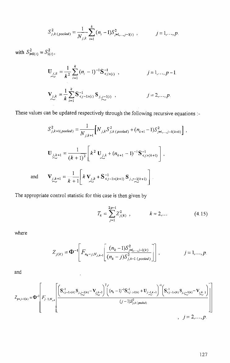
^J,k(pooled) - ~ Au^"i~^^^J»l,...J-Ki N j.k ,=1 y = i,---,/?
with i>i.o(,) - i J ^ , ) ,
j = l,...,p-l.
I 7 = 2,...,/?.
These values can be updated respectively through the following recursive equations
C.2 "^ J,k+K pooled) ~ \ r \^J,k^J,k (pooled)+("k+l l ) ' ^ ; . l , . . , ; - l ( / t+ l )
U j,k+l (k + iy
f^"^j,k+in,,,-i)-'s:],,,.
and V j,k+l k + l ^ ^j,k + ^<y- l> ( ; t+ l ) S ; J '-l(yt+l)
The appropriate control statistic for this case is then given by
2/7-1
^k = Zu ^Kk) ' /=1
k = 2. (4.15)
where
ZjXk) = ^ R "k-r'^j,k-i (« . - i )^ ; . i . . . . , ; - •l(^)
("yfc J)^J,k-l (pooled) j=l,...,p.
and
Wm=^' ^J-^-Nj., 0 ^)^j.k( pooled)
, 7 = 2,...,/?.
127
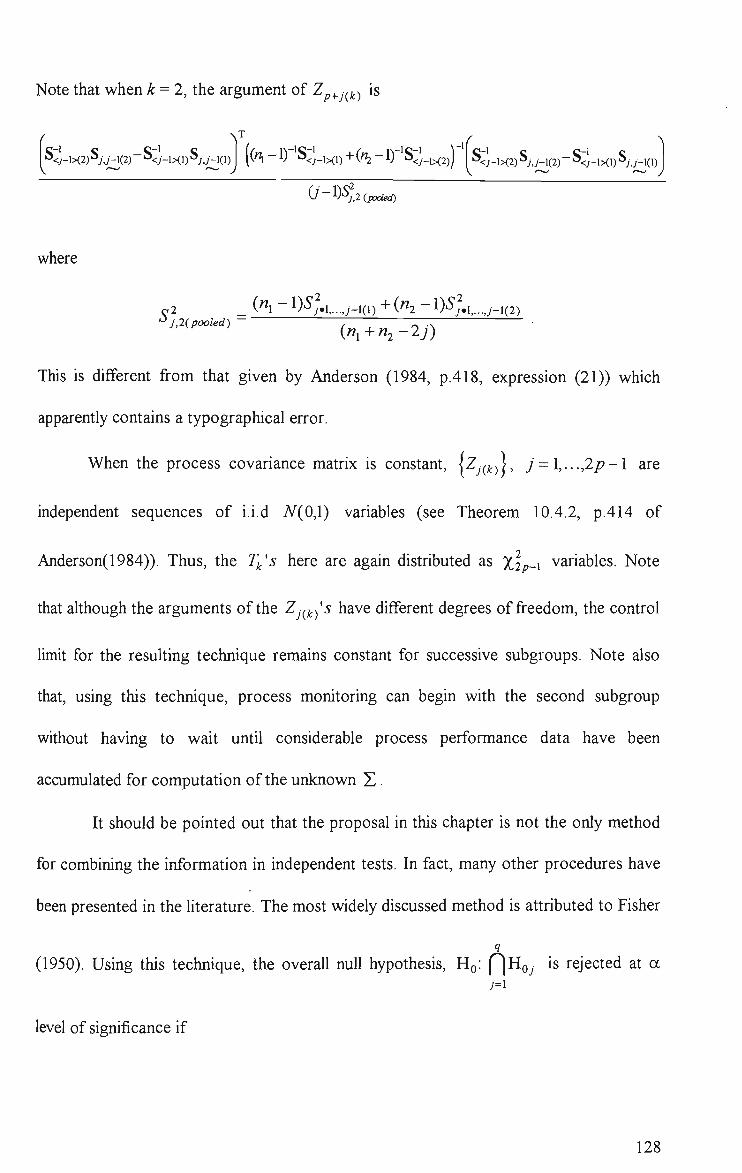
Note that when k = 2, the argument of Z + v x is
Kj-\>Q-) ;.;-l(2) S<;-I>(1) Sy.y_,(i) I ((«i -1) 8<y_]>(,) + (/^ -1) 'S<J._^2)) ^<j-\>{2) S;.;-l(2)- S^-IXD S;.y_l(l)
(7-1)5?.:
where
p2 _ (^1 ~l)'^y«l,...,/-l(l) + ( ^ 2 ~0'^>1,..,;-1(2) •^ j,2(pooled) - /-v, _i_ :« O V\
( « i+»2-27)
This is different from that given by Anderson (1984, p.418, expression (21)) which
apparently contains a typographical error.
When the process covariance matrix is constant, |Zy(^)>, j = l,...,2p-l are
independent sequences of i.i.d JV"(0,1) variables (see Theorem 10.4.2, p.414 of
Anderson(1984)). Thus, the Tj^'s here are again distributed as xlp-i variables. Note
that although the arguments of the Zj^^i^^'s have different degrees of freedom, the control
limit for the resulting technique remains constant for successive subgroups. Note also
that, using this technique, process monitoring can begin with the second subgroup
wUhout having to wait until considerable process performance data have been
accumulated for computation of the unknown E .
It should be pointed out that the proposal in this chapter is not the only method
for combining the information in independent tests. In fact, many other procedures have
been presented in the Uterature. The most widely discussed method is attributed to Fisher
(1950). Using this technique, the overaU nuU hypothesis, UQ. f^Hoj is rejected at a
level of significance if
128

-22lnP,>X^,,i_„
where P/s denote the /?-values of the mdependent tests for the q sub-hypotheses
Hoy's. Another common procedure is based on the minimum significance level of the
independent tests as suggested by Tippett (1931). For this method, HQ is rejected at a
level of significance if
xmn{P„...,P^}<l-{l-afr
We note that our procedure of forming a smgle control statistic is actually a special case
of Lancaster's (1961) method which rejects HQ at a level of significance if
where r~J^{») and 7" ^ denote respectively the inverse and the lOOorth percentile of a
Gamma distribution with parameters (v, 1/2). This is so when Vy = 1/ 2 for 7 = 1,...,^. A
review of these and other test combination procedures is given in Folks (1984). Previous
studies indicate that Fisher and Tippett methods are good omnibus procedures if the test
statistics for the sub-hypotheses are independent chi-square or F variables. However, the
resuUs of these studies do not apply in the present context since the problem here does
not involve non-central chi-square or /^variables under the alternative hypothesis.
In this chapter, no attempt has been made to determine the optimal choice of
combination method except for the simulation study of the relative performance of
Fisher, Tippett and the proposed procedures as reported in section 4.5. Other methods
such as the weighted average of normal scores obtained from independent statistics and
the weighted version of Fisher's method are not considered due to the arbUrary choice of
129

the weighting constants. If equal weights are used, the former is equivalent to the
commoly called Inverse Normal procedure. This technique, which is based on the sum,
2p-l
^Zj^j^) for the problem under consideration, is expected to be ineffective for the
reason given earlier. Similarly, the Bayes or likelihood ratio procedures derived by
Koziol and Periman (1978) and Marden (1982) for combining independent noncentral
chi-square and F statistics respectively are inappropriate since the aUernative hypotheses
in question do not fit the specified models. Even if the models are appropriate,
determination of critical values for the resuhing techniques can be quUe involved. The
same is true for the other techniques not considered here including those based on the
sum of chi statistics (see Koziol et al.(1978)).
4.4 Rank-Deficient Problem
As stated earlier, the proposed techniques are applicable only if the sample size
exceeds the number of jointly monitored variables or the sample covariance matrix is of
fiiU rank. However, these techniques can be adapted to the rank-deficient situations as
described below.
For mathematical convenience, suppose that samples of equal size n are used
where n<p. In this case, simply transform the sample covariance matrices, 8(, '5 to
matrices of reduced dimension, W^,)' as follows :
W(-;) = A8(,)A
where A is a fiiU rank (n-l)xp matrix of constants. By theorem 3.3.7 of Srivastava et
al.(1979).
130

(«-l)W(,^~fF^i(«-l,AEA^).
FoUowing this transformation, the problem becomes one that checks the constancy of the
variance-covariance matrix, E through AEA^. The same methods of decomposition
and combination of the resuhing independent statistics can then be applied to the fiiU
rank matrices, 'W(,)'5 and the associated likelihood ratio statistics for the known and
unknown E cases respectively. Although dimensional reduction inevitably leads to some
loss in information and the choice of A is somewhat arbUrary, this approach can be used
irrespective of the sample size (provided n>2) and valid control limits can be easily
located.
Notice that as a special case of the transformation, W ,) becomes the sample
covariance matrix of the first n-l quality characteristics if
^~\}(n~l)x(n-l)^ "(«-l)xp j •
This choice of A is undesirable since U sacrifices the information regarding the last
p-n + l variables. If E is known, a reasonable choice of A is that whose rows consist of
the normalized eigenvectors corresponding to the largest n-l eigenvalues, A,i,...,A,„_i, of
E . Under this transformation, W y) becomes the sample covariance matrix of the first n-
1 principal components and AEA^ = A = diag(Xi,...,X„_i).
Other methods that can be used for the known E case include those which are
based on all the principal components, any set of Unearly independent combinations of
the quality variables and the union-intersection principle (Srivastava et al. (1979)).
131
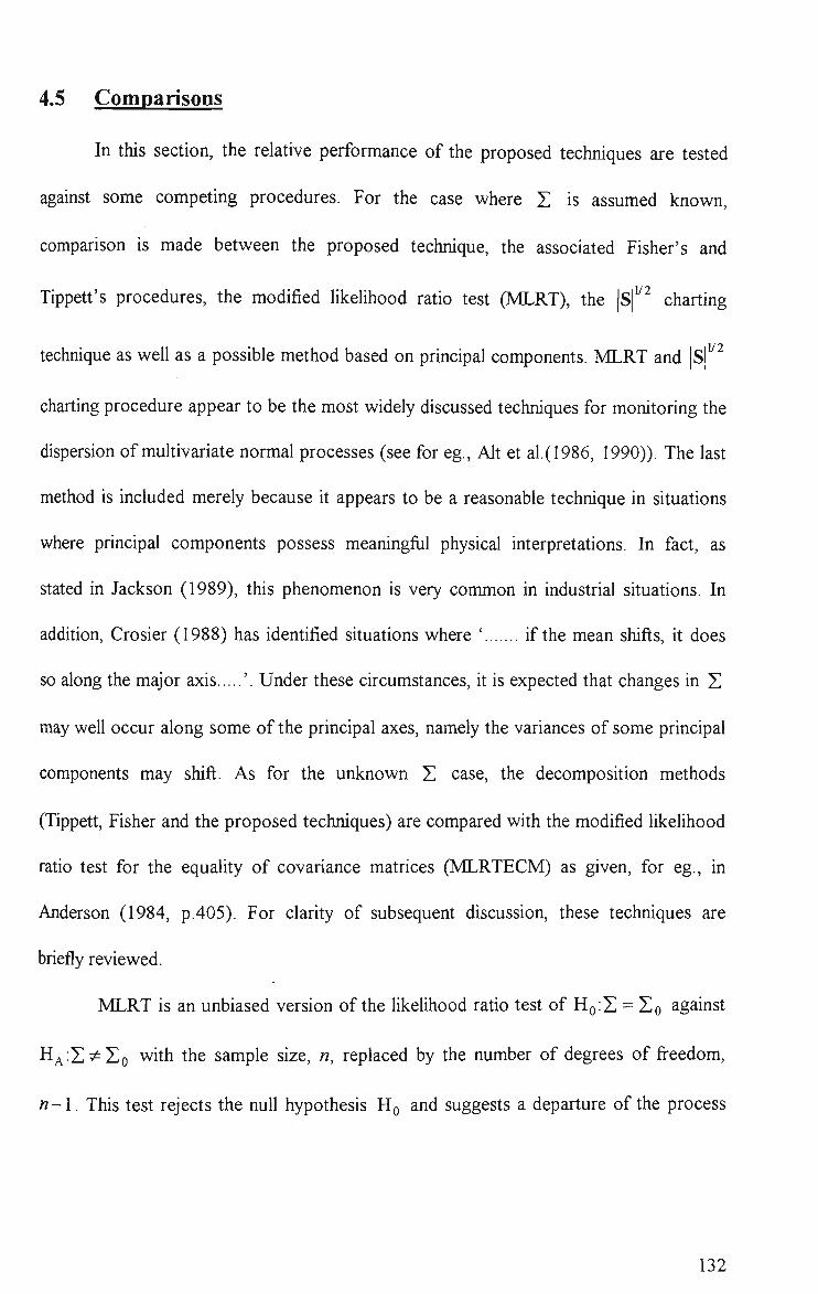
4.5 Comparisons
In this section, the relative performance of the proposed techniques are tested
against some competing procedures. For the case where E is assumed known,
comparison is made between the proposed technique, the associated Fisher's and
Tippett's procedures, the modified likelihood ratio test (MLRT), the IS]' ^ chartmg
technique as weU as a possible method based on principal components. MLRT and |8|^^
charting procedure appear to be the most widely discussed techniques for monitoring the
dispersion of multivariate normal processes (see for eg., Alt et al.(1986, 1990)). The last
method is included merely because it appears to be a reasonable technique in situations
where principal components possess meaningfiil physical interpretations. In fact, as
stated in Jackson (1989), this phenomenon is very common in industrial situations. In
addition. Crosier (1988) has identified situations where ' if the mean shifts, it does
so along the major axis '. Under these circumstances, U is expected that changes in E
may well occur along some of the principal axes, namely the variances of some principal
components may shift. As for the unknown E case, the decomposUion methods
(Tippett, Fisher and the proposed techruques) are compared wUh the modified likelihood
ratio test for the equality of covariance matrices (MLRTECM) as given, for eg., in
Anderson (1984, p.405). For clarity of subsequent discussion, these techniques are
briefly reviewed.
MLRT is an unbiased version of the likelihood ratio test of HQIE = EQ against
H^iE^^^Eo 'with the sample size, n, replaced by the number of degrees of freedom,
n-l. This test rejects the null hypothesis HQ and suggests a departure of the process
132

covariance matrix from the standard or the known value Eo when the test or control
statistic, W* exceeds Wp„a where
PF* =- /?(«- l ) - («- l ) ln |8 | + («-l)ln|EoI+ («-l)tr(Eo S) . (4.16)
a and Wp„a^ denote respectively the false signal rate and the upper 100 a th percentage
point of W* which depends on p and n. The distributional theory involved with this
technique is prohibitively complicated thus limiting Us practicality. Although W* can be
approximated by a chi-square distribution with ^-^—- degrees of freedom when « is
large, and the exact upper 1% and 5% percentage points of W* have been tabulated, for
example, in Anderson (1984), for/? - 2(1)10 and various values of «, these may be of
little value in the context of control charting. In practice, the control or monitoring
procedures are likely to be based on samples not sufficiently large to justify the use of the
chi-square approximation. Besides, it may be preferable to have a control technique wUh
false signal rates considerably smaUer than 1% or 5%. Although MLRT is admissible
(Giri (1977), p. 186), it wiU be seen later that this technique is inferior to the proposed
technique for all of the cases considered.
The other competing procedure is based on the use of the square root of the
generalized sample covariance matrix, |8j . The resulting chart can be regarded as a
I |1^2
muhivariate analogue of the univariate S chart. When p = 2, |S| is distributed as a
scaled chi-square variable under the stable or in-control multivariate normality
assumption (Anderson (1984), p.264). Thus, control Umits may be set at
LCL = l-^ol X2(n-2),a/2
2(«-l)
133
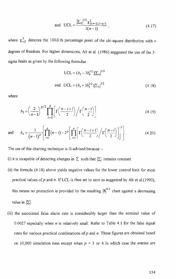
and UCL = _ 1- 01 X2(«-2),l-a/2
2(«-l) (4.17)
where Xv,5 denotes the 1005 th percentage point of the chi-square distribution with v
degrees of freedom. For higher dimensions, Alt et al. (1986) suggested the use of the 3-
sigma limits as given by the following formulae :
LCL=(Z>3-3^»f)|Eor
l/2xlv^ |V2 and UCL = (Z)3+3Z>r)|E (4.18)
where
2 v/^A / = 1
v«-iy . 2 J
n-l (4.19)
and ^ = — ^ ff(«-/)-2^ n ( = 1
« - z+r 2 J
-\2
(4.20)
The use of this charting technique is iU-advised because :-
(i) U is incapable of detecting changes in E such that |E| remains constant.
(ii) the formula (4.18) above yields negative values for the lower control limit for most
practical values of/? and n. If LCL is thus set to zero as suggested by Alt et al.(1990),
this means no protection is provided by the resulting |8| chart against a decreasing
value in |E| .
(iu) the associated false alarm rate is considerably larger than the nominal value of
0.0027 especially when n is relatively smaU. Refer to Table 4.1 for the false signal
rates for various practical combinations of/? and n. These figures are obtained based
on 10,000 simulation runs except when /? = 3 or 4 in which case the entries are
134
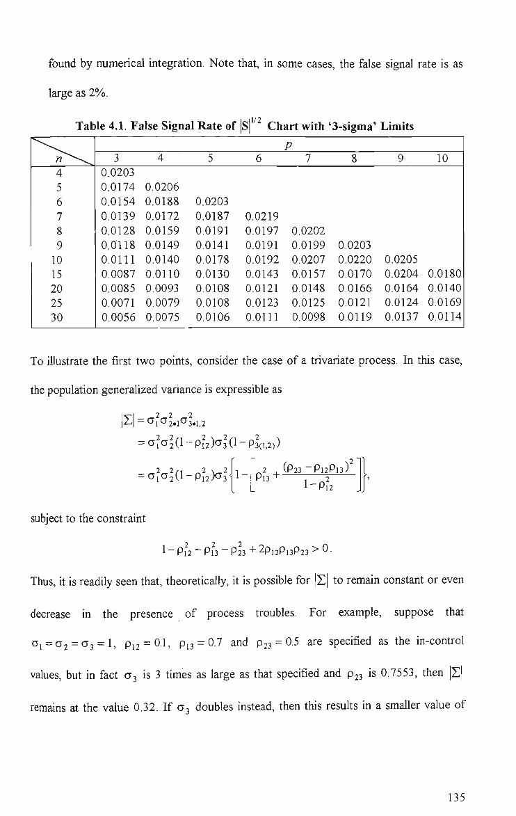
found by numerical integration. Note that, in some cases, the false signal rate is as
large as 2%.
1/2 Table 4.1. False 8ignal Rate of S Chart with '3-sigma' Limits
W'^^^v^
4 5 6 7 8 9 10 15 20 25 30
P 3
0.0203 0.0174
0.0154
0.0139 0.0128 0.0118 0.0111 0.0087 0.0085 0.0071 0.0056
4
0.0206
0.0188
0.0172
0.0159 0.0149 0.0140
0.0110 0.0093 0.0079 0.0075
5
0.0203 0.0187
0.0191 0.0141 0.0178 0.0130 0.0108 0.0108 0.0106
6
0.0219 0.0197 0.0191 0.0192 0.0143 0.0121 0.0123 0.0111
7
0.0202 0.0199 0.0207 0.0157 0.0148 0.0125 0.0098
8
0.0203 0.0220 0.0170 0.0166 0.0121 0.0119
9
0.0205 0.0204 0.0164 0.0124 0.0137
10
0.0180 0.0140 0.0169 0.0114
To illustrate the first two points, consider the case of a trivariate process. In this case,
the population generalized variance is expressible as
IVl ^ 2 ^ 2 2 H = ^1^2.1^3.1,2
= CTja^(l-Pl2)03(l-p3(l,2))
= c5{ai{l-Q{2)^U 1- 2 , (P23-P12P13) Pl3 " , ^2
I -P12
subject to the constraint
1 - 9n - 9x3 - P23 + 2pi2pi3p23 > 0 •
Thus, U is readily seen that, theoretically, U is possible for |E| to remain constant or even
decrease in the presence of process troubles. For example, suppose that
0 = 02=03 = 1, pi2 = 0.1, Pi3 = 0.7 and P23 = 0.5 are specified as the in-control
values, but in fact Oj is 3 times as large as that specified and P23 is 0.7553, then |E|
remains at the value 0.32. If a . doubles instead, then this resuUs in a smaller value of
135

|E|. In either case, the departure is unlikely to be 'picked up' by the |8|^^ charts
presented by Alt et al.(1986).
It is perhaps worth noting that, for/? = 3 or 4, control limits for the 181 ^ chart
can be obtained numerically at any desired a level. In this case, the control limits are
given by
LCL= .^«^^ „ n | l o r ' and UCL= ^'-'=^'^ \ z r (4.21) 2^^(«-l)^^^' °' 2^-^(«-l)^^^' °' ^ ^
where 5 is a numerical solution to the integral equation,
j G2(.-p){kJx^'-'~^'')g^p_2^„_p,2ix)dx = 5 . (4.22)
0
The notation g^(«) and G^(«) here denote respectively the probability density and the
distribution fiinction of a chi-square variable with v degrees of freedom, k^ is obtained in
this manner using Mathematica version 2.2 (Wolfram (1991)) and is given to 4
significant digits in Table 4.2 for/? = 3 and 4, and various combinations of 6 and n.
The last technique considered for the known E case is aimed at changes of E
along the principal axes. It involves charting the sum of the standardized variances for
the principal components, abbreviated hereafter as SSVPC, which is known to be
distributed as a scaled chi-square variable under the multivariate normal assumption with
the hypothesized E . The value of SSVPC may be calculated from the familiar equivalent
statistic («-1)^^(8Eo/ (see Appendix A.6). Note that, unlike all other control
procedures considered in this section, this technique is applicable even in situations
where n< p. It has also been shown by Kiefer and Schwartz (1965) that U is admissible.
Although separate momtoring of the variances for the different principal components is
136

possible, this is not considered due to the large number of charts to be kept when p is
large. It is also for meaningfiil comparison with other techniques involving a smgle chart
that separate monitoring of the variances is not considered. However, in practice, it is the
recommendation that these individual variances be retained in order to faciUtate the
mterpretation of out-of-control signals from the SSVPC charts.
J»i
^
3
4
4 5 6 7 8 9 10 15 20
5 6 7 8 9 10 15 20
Table 4.2. 1 |J/2
|8| Control Chart Factor, A^ S
0.00135
.0034
.1513
.6842 1.673 3.117
5.050 7.417 25.39 52.80
.0108
.5297
2.620 6.981
14.10 24.36 132.1 350.0
0.0025
.0063
.2082
.8573 2.007
3.652 5.780 8.375 27.76 56.65
.0200
.7308 3.303 8.427 16.60 28.13 146.0 379.1
0.005
.0126
.2994 1.112 2.473 4.367 6.770 9.659 30.73 61.51
.0401 1.055 4.318 10.49 20.03 33.30 164.1 416.6
0.995
20.98 34.48 48.15 62.25 76.85 91.92 107.5 191.7 285.6
90.46 169.3 260.4 364.3
480.6 609.1 1427 2522
0.9975
24.48 38.87 53.81 68.86 84.35 100.3 116.7 204.9 302.6
108.0 195.9 296.2
409.6 535.7 674.2 1546 2703
0.99865
27.73 43.18 58.90 74.70 91.01 107.7 124.8 216.5 317.4
124.5 220.5 329.1 450.4
585.0 732.7 1652 2862
In the absence of prior information about E, Alt et al.(1990) suggested using the
,|l/2 MLRT and |S| control charts wUh the unknown process dispersion parameters in
(4.16) and (4.18) being replaced by some unbiased estimates based on current
production data. Under these circumstances, the data used for estimating the unknown
parameters are likely to be either small or moderate data sets. Accordingly, the false
signal rates of the resuhing techniques are not fixed but instead vary stochastically wUh
the parameter estimates. This causes some difificuUies when a comparison is to be made
137
between these and the proposed technique. Thus only MLRTECM, which was originaUy
proposed in the context of hypotheses testing, is considered.
The criterion for MLRTECM is
W = [EA2, - ^ J ln|s^,,,,^|- ^ (« , . -l)ln|S(,)| (4.23) /=i
where S ,-,, «, and 8 ^ ^ ^ denote respectively the rth sample covariance matrix, Us
associated sample size and the pooled covariance matrix based on the q samples. It was
shown by Anderson (1984) that U is an admissible test if «, >2/?- l , i = l,...,q. For
equal sample sizes n^=n, this test rejects the null hypothesis that all the q samples are
drawn from populations wUh the same covariance matrix if W> W^p„^ where W^p^^
denotes the critical value at the 100a% significance level. The upper 5% points of W
have been tabulated, for example, in Anderson (1984) for various combinations of/?, q
and n. There are two problems wUh the use of MLRTECM in the context of SPC. The
existing tables for the percentiles of W are incomplete in regard to other values of/?, q, n
and a which are required for SPC applications. Besides, successive values of W are
correlated and thus the in-control behaviour of the resulting technique is somewhat
unpredictable. However, it is found that ignoring this issue does not appear to have any
remarkable effect on the overall false signal rate. Therefore, a reasonable comparison can
stUl be made between this and the decomposition procedures by using the same a value
for all the methods.
It is shown in Appendices A.4, A.6 and A. 7 respectively that the statistical
performance of MLRT, SSVPC and MLRTECM (for a step shift in E from EQ to Ej)
_ i _ i _ i
depend on the eigenvalues, Xi,...,X of E o ^ S i E o \ or equivalently, of EQ S I or
138
I l E o ^ whereas that of the |8| chartmg technique depends on EQ and Ei only
through the product of these eigenvalues, X{X2...Xp (see A.5). Note that X{X2...Xp
represents the ratio of the 'equal-content' volumes of the process ellipsoids
corresponding to Ei and EQ respectively. In addition, Nagao (1967) and Das Gupta
(1969) independently showed that the power fiinction of the MLRT is monotonically
increasing with respect to |>-,-l| V/. Furthermore, note that the MLRT, SSVPC,
I l l /2
MLRTECM and |8| charting procedures are invariant w.r.t. the transformation
X* = r x + p where T is any nonsingular matrix. This is not true with the
decomposition techniques except when Y is diagonal. By letting F = diag\-^,...,^\, it
is readily seen that the values of Fisher, Tippett and the proposed statistics are the same
whether they are computed from the covariance or correlation matrix (see A. 8 and A. 9),
and this is also true for the other invariant procedures considered above. However,
difficulties arise when an attempt is made to compare their operating characteristics,
since the statistical properties of the decomposUion techniques do not appear to be
completely determined by the eigenvalues of E Q ^ E I E O ^ - TO provide a 'sensible'
comparison, it is therefore necessary to consider several possible combinations of EQ
and El which yield the same eigenvalues Xi,...,Xp (and thus the same eigenproduct
X{X2...Xp) and determine the 'average' performance of the decomposition techniques
relative to that of the competing procedures. Note, however, that only HQ'S in the form
of correlation matrix need to be considered.
A somewhat systematic way of studying the relative performance of the various
competing techniques is to use several arbitrary orthonormal matrices F 's that
139

diagonalize E Q ^ ^ S I S O ^ ^ giving the same diagonal matrix of eigenvalues,
A = diag(Xi,...,Xp). For a given EQ , A and T , Ei is then determined from
Ei = Err^ArEr.
Amongst others, the orthonormal matrix that diagonaUzes EQ , T = FQ is used. This
corresponds to situations where the shift is along the principal axes, namely, the
variances of some principal components either increase or decrease. Under these
circumstances, the eigenvalues of EQ^^ E I EQ^^ are the ratios of variances for the
principal components, after and before the shift, and hence the control performance of
MLRT, MLRTECM, SSVPC and |8| depend on them (see A. 10). Note that if the
eigenvalues of E Q ^ ^ E I E Q ^ ^ are identical, then Ei is the same irrespective of F . In
this case, Ei = A-EQ where X is the common eigenvalue. This situation may occur in
practice as a consequence of all variances increasing proportionally and tUe correlational
structure of the variables remaining the same (see Healy (1987)).
The techniques considered for the known E case above are compared on the
basis of the probability of detecting a persistent shift in the process covariance matrix
from Eo to El . It is assumed that this change, as well as the shift in the process mean
vector if any, occurs somewhere during the time interval between the sampling of two
adjacent subgroups. Accordingly, the covariance matrices for samples or subgroups
taken after the shift are characterized by a common distribution and the mean shift has no
effect on this distribution. Of course, if desired, the average run lengths (ARLs) of the
various techniques can be determined as the reciprocals of their corresponding
probabilities of detection. As for the unknown E case, a more complete profile of the
run length (RL) properties is required. This is because the out-of-control RL
140

distributions of aU techniques under consideration are not geometric so that the ARL is
not a suitable performance criterion (see Quesenberry (1993,1995d)). Furthermore, since
these techniques estimate the in-control dispersion parameters sequentially from the
current data stream and the efficiency of these estimates increases as more data are
incorporated into the computations, it can be expected that their RL performance
depends on when the shift takes place. As such, the relative performance of MLRTECM,
Fisher, Tippett and the proposed techniques are evaluated based on Pr(7?L < k) for a
step change in E after the rth subgroup, for various combinations of r and k.
The resuUs for the known E case are tabulated in Tables 4.3, 4.4 and 4.5
respectively for the cases where (p = 3, n = 4), (p = 4, n = 5) and (/? = 5, « = 8). These
are based on simulations consisting of 5000 iterations each. Thus, the estimated
Pr(l-Pr) maximum standard error of the resuUs is J—^^ « 0.0071 which occurs when the
V 5000
estimated probability, Pr = 0.5. For the unknown E case, the results are based on 2000
simulation runs each (with maximum standard error w 0.0112) and these are shown in
Tables 4.6, 4.7 and 4.8 respectively for (p = 2, n = 3),(p = 3,n = 4) and (p = 4, « = 5).
Here, U is assumed that the control procedures are based on subgroups of equal size, n.
The false signal rate associated with each of the control schemes is fixed at 0.0027, in
line with the tradional control charting approach. Note that the control Umits for MLRT
and MLRTECM are obtained to sufficient accuracy using the work of Davis and Field
(1971). The control Umits for the | s f ^ chart are determined from Table 4.2 for/? = 3, 4
and by means of simulation consisting of 100,000 Uerations for/? = 5 and « = 8. Note
also that 2-sided control limits with equal significance level on each side are used with
SSVPC.
141
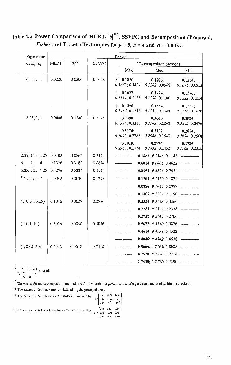
,|l/2 Table 4.3. Power Comparison of MLRT, \S\"'\ S8VPC and Decomposition (Proposed, Fisher and Tippett) Techniques for/? = 3, « = 4 and a = 0.0027.
Eigenvalues
ofEo'Si
4, 1, 1
6.25, 1, 1
2.25,2.25, 2.25
4, 4, 4
6.25, 6.25, 6.25
'(1,0.25,4)
(1,0.16,6,25)
(1,0.1,10)
(1,0.05,20)
MLRT
0.0226
0.0888
0.0102
0.1326
0.4276
0.0342
0.1046
0.3026
0.6062
,;l/2
0.0206
0.0340
0.0862
0.3182
0.5234
0.0030
0.0028
0.0040
0.0042
SSVPC
0.1668
0.3374
0.2140
0.6674
0.8944
0.1298
0.2890
0.5036
0.7410
Power
' Decomposition Methods
Max Med Min
* 0.1820; 0.1286; 0.1660; 0.1494 <?.7202; 0.0968 0
t 0.1622; 0.1474; 0.1314;0.U3S 0.7250; 0.1100 0
t 0.1390; 0.1334; 0.747<J; 0.1216 0.7752; 0.1044 0
0.3490; 0.3060; 0.3336; 0.3210 0.3168; 0.2868 0
0.3174; 0.3122; 0.3092; 0.2786 0.2906; 0.2540 0.
0.3010; 0.2976; 0.2988; 0.2754 0.2832; 0.2452 0
0.1254; 7074; 0.0832
0.1346; 7222; 0.1034
0.1262; 7775; 0.1036
0.2926; 2842; 0.2476
0.2874; 25P4; 0.2508
0.2936; 2768; 0.2356
0.1688
0.6014
0.8664
0.1704
0.0886
0.1306
0.3324
0.2786
0.2732
0.5622
0.4610
0.4846
0.8066
0.7528
0.7430
0.1546; 0.U4S
0.6006; 0.4622
0.8524; 0.7634
0.7J70; 0.1824
0.7044; 0.0998
0.7752; 0.1190
0.3148; 0.3366
0.2522; 0.2358
0.2744; 0.2706
0.5580; 0.5826
0.45iS; 0.4522
0.4542; 0.4538
0.7702; 0.8008
0.752(5; 0.7214
0.7i7(J; 0.7290
n= I" 1
0.75
la45
a7s 1
09
0.45"
OS
1 J
is used.
The entries for the decomposition methods are for the paiticulai permutations of eigenvalues enclosed within the brackets.
* The entries in 1st block are for shifts along the principal axes.
t The entries in 2nd block are for shifts determined by r=
X The entries in 3rd block are for shifts determined by
1 / ^
U,l2 11 Je
0.44
0.78
0.44
uji -vji i/Ji
0.85 -052 ao6
uji 0
-2/^6
0:27 I
035 -090
142

ll/2 Table 4.4. Power Comparison of MLRT, |8| , 8SVPC and Decomposition (Proposed,
Fisher and Tippett) Techniques for/> = 4,« = 5 and a = 0.0027.
Eigenvalues
ofZo'Si MLRT All SSVPC
Power
' Decomposition Methods
Max Med Min
4, 1, 1, 1 0.0154
6.25, 1, 1, 1 0.0688
2.25,2.25,2.25,2.2^ 0.0110
4 ,4 ,4 ,4 0.1914
6.25,6.25,6.25,6.25| 0.6144
b "(0.25,0.25,4,4)
(1,1,0.16,6.25)
(0.16,0.16,6.25,6.25)
(1,1,0.1,10)
0.0810
0.0932
0.3412
0.3040
0.0214
0.0346
0.1358
0.4480
0.6968
0.0040
0.0012
0.0038
0.0036
Io =
( 1 0.5 0.9 0.6^
0.5 1 0.2 0.7 is used.
0.9 0.2 t 0,4
1,0.6 0.7 0.4 1 J
0.1712
0.3812
0.3802
0.8846
0.9842
0.3218
0.3114
0.6570
0.5662
* 0.1782; 0.1664; 0.1452; 0.7522; 0.2084 0.7574; 0.1665 0.7iPO; 0.1538
t 0.1850; 0.1530; 0.1326; 0.7725; 0.1876 0.7452; 0.1511 0.7225; 0.1258
% 0.1656; 0.1480; 0.1350; 0.7772; 0.1416 0.1331; 0.1292 0.1138; 0.1004
0.3996; 0.3790; 0.3502; 0.3838; 0.4270 0.3546; 0.3653 0.3428; 0.3570
0.4010; 0.3373; 0.3320; 0.3602; 0.4076 0.3370; 0.3312 0.3228; 0.2942
0.3850; 0.3448; 0.3280; 0.3584; 0.3380 0.3158; 0.3276 0.3008; 0.2694
0.2970; 0.2762
0.8300; 0.8528
0.9746; 0.9680
0.4116; 0.4088
0.4150; 0.3664
0.4466; 0.4352
0.3616; 0.3570
0.3742; 0.3622
0.3380; 0.3074
0.7208; 0.7122
0.7358; 0.6858
0.7587; 0.7552
0.6116; 0.5972
0.6064; 0.5990
0.5868; 0.5440
0.1686
0.6470
0.9186
0.3726
0.3478
0.3434
0.3778
0.3454
0.3754
0.6816
0.6602
0.6340
0.5984
0.5902
0.6006
' The entries for the decomposition methods are for the particular permutations of eigenvalues enclosed within the brackets.
* The entries in 1st block are for shifts along the principal axes. r 1/2 1/2 1/2
t The entries in 2nd block are for shifts determined by
t The entries in 3rd block are for shifts determined by
1/2
1/^2 -I/V2 0 0
l/Vs 1/V6 -2/V6 0 ,1/ 12 i/Vi2 i/i/iz -21 Jn)
(0S9 0.07 0.09 0.06' -0.11 OJO 058 0J5 -0.08 0.71 -019 0.04
10.06 0J5 0.68 -0.72;
143
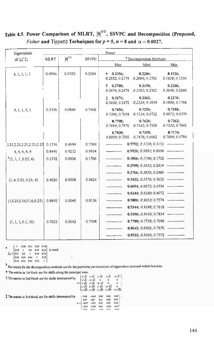
11/2 Table 4.5. Power Comparison of MLRT, |8| , 8SVPC and Decomposition (Proposed,
Fisher and Tippett) Techniques for/; = 5, « = 8 and a = 0.0027.
Eigenvalues
ofSo'Si MLRT |S| 1/2 SSVPC
Power
* Decomposition Methods
Max Med Min
4 ,1 ,1 ,1 ,1 0.0946 0.0320 0.2604
9,1,1,1,1 0.5336
2.25,2.25,2.25,2.25,2.25
4 ,4 ,4 ,4 ,4
''(1,1,1,0.25,4)
(1,4,0.25,0.25,4)
(1,6.25,0.16,0.16,6.25)
(1,1,1,0.1.10)
0.1356
0.8440
0.1332
0.4620
0.8692
0.7622
0.0844 0.7406
0.4694
0.9232
0.0026
0.0008
0.0040
0.0042
0.7560
0.9954
0.1766
0.4624
0.8156
0.7398
* 0.2356; 0.2206; 0.1926; 0.2052; 0.2174 0.2004; 0.1702 0.7858; 0.1550
t 0.2788; 0.2450; 0.2206; 0.2674; 0.2474 0.2782; 0.2302 0.2048; 0.2040
% 0.3174; 0.2362; 0.2176; 0.3020; 0.2472 0.2224; 0.1834 0.1896; 0.1768
0.7456; 0.7256; 0.7188; 0.7505; 0.7058 0.7724; 0.6722 0.5872; 0.6370
0.7708; 0.7626; 0.7262; 0.75P4; 0.7476 0.7542; 0.7208 0.7220; 0.7042
0.7838; 0.7350; 0.7174;
0.8050; 0.7202 0.7478; 0.6902 0.7005; 0.6784
0.5792; 0.5738; 0.3152
0.9926; 0.9882; 0.8998
0.1866; 0.7740; 0.1702
0.2990; 0.2932; 0.2414
0.2766; 0.2850; 0.2486
0.5422; 0.5576; 0.3652
0.6694; 0.6672; 0.4354
0.6244; 0.6160; 0.4072
0.9006; 0.9052; 0.7574
0.9344; 0.9398; 0.7618
0.9396; 0.9470; 0.7854
0.7780; 0.7758; 0.7098
0.8642; 0.8502; 0.7676
0.8532; 0.8360; 0.7972
1 0.58 051 039 0.46' 0j8 1 0.6 039 032 is used. Oil 0.6 1 0.44 0.43
039 039 0.44 1 052
0.46 032 0.43 052 1
Tlie entries for the decomposition methods are for the paiticulai permutations of eigenvalues enclosed within brackets.
* The entries in 1st block are for shifts along the principal axes. t The entries in 2nd block are for shifts determined by \/.^ \/Ji \ o o
r= 1/76 i/Vs -2/1/6 0 0 1/JI2 vJn \ijn -)ijn o ,1/,^ 1/,/M I/TM UM /TZO,
t The entries in 3rd block are for shifts determined by 0.88 -0.48 0.00 0.00 0.00' 0.47 0.87 OJl 0.08 0.07
-0.07 -Oi3 052 059 059 -0.02 -0.03 0«5 -034 -0.41 nnn nnn ni\A nft n/:Q
144

Table 4.6 Pr(RL < k) for a Change in Z after the rth Subgroup, by MLRTECM and Decomposition (Proposed, Fisher and Tippett) Techniques for p = 2, n = 3 and a = 0.0027.
Eigenvalues
of So ' Si MLRTECM
' Decomposition Methods
Max Min
4, 1 10
20
9, 1 10
4, 4
6.25, 6.25
9, 9
20
10
20
10
20
10
20
10
10
10
10
5 10 5
10 5
10 5
10 5
10 5
10
0.0110
0.0205
0.0125
0.0165
0.0360
0.0525
0.0485
0.0970
0.0265 0.0425 0.0330 0.0645 0.0675 0.1090 0.0940 0.1905 0.1465 0.2270 0.2365 0.4120
* 0.7275 (0.1230) 0.1315 0.0955 (0.0945) 0.0705 t 0.1675 (0.1745) 0.1925 0.1040 (0.1185) 0.0990 t 0.1610 (0.1725) 0.1730 0.0895 (0.0930) 0.0800
0.1830 (0.1840) 0.1835 0.1350 (0.1370) 0.0965 0.2025 (0.2185) 0.2490 0.1505 (0.1605) 0.1210 0.7P55 (0.2060) 0.1985 0.75P0 (0.1385) 0.1150 0.2265 (0.2480) 0.2415 0.7955 (0.1950) 0.1475 0.2515 (0.2775) 0.3050 0.1935 (0.2045) 0.1870 0.2180 (0.2370) 0.2320 0.1975 (0.1915) 0.1480 0.3315 (0.3345) 0.3285 0.2810 (0.2845) 0.2400 0.3290 (0.3490) 0.3675 0.2950 (0.2955) 0.2715 0.3270 (0.3545) 0.3720 0.3035 (0.3050) 0.2530 0.4730 (0.4915) 0.4960 0.3445 (0.3470) 0.2445 0.4635 (0.5055) 0.5450 0.2990 (0.3035) 0.2490 0.4445 (0.4670) 0.5225 0.3120 (0.3140) 0.2270 0.5360 (0.5675) 0.5780 0.3920 (0.3855) 0.2855 0.5360 (0.5740) 0.6150 0.4065 (0.4065) 0.3270 0.5355 (0.5620) 0.5940 0.4090 (0.4045) 0.3240 0.6510 (0.6675) 0.6760 0.5475 (0.5490) 0.4175 0.7210 (0.7425) 0.7680 0.5800 (0.5845) 0.5130 0.6565 (0.6805) 0.7105 0.5685 (0.5640) 0.4530 0.7760 (0.7980) 0.8085 0.7030 (0.6955) 0.5535 0.8055 (0.8245) 0.8490 0.7790 (0.7205) 0.6295 0.7765 (0.8045) 0.8090 0.6955 (0.6920) 0.5730
0.5540(0.3575)0.3200 0.4055(0.4160)0.3815 0.5035 (0.5135) 0.4730 0.5570(0.6705)0.6340 0.5950(0.6110)0.5445 0.5555(0.6820)0.6265 0.8275(0.8405)0.7810 0.9240(0.9320)0.8865 0.8025(0.8100)0.7370 0.8570(0.8535)0.7930 0,9550(0.9725)0.9450 0.9745(0.978510.9780
Io = 1 0.5
05 1 is used.
* The entries in 1st row are for shifts along the principal axes. f-0.996 0.094^
t The entries in 2nd row are for shifts determined by T= 1,-0.094 -0996J
f0.189 0982) I The entries in 3rd row are for shifts determined by F = A . oo '
145

Table 4.7. Pr(RL < k) for a Change in Z after the rth Subgroup, by MLRTECM and Decomposition (Proposed, i w/zer and Tippett) Techniques for/; = 3, « = 4 and a = 0.0027.
Eigenvalues
of l o ' S , MLRTECM
' Decomposition Methods
Max Med Min
4,1,1 10
10
20
9,1,1
4,4,4
9,9,9
10
10
20
10
20
10
20
10
10
5 10 5 10 5 10 5 10
' I 0.75 0.45'
0.75 1 09
,0.45 0,9 1 ,
is used.
0.0100
0.0170
0.0135
0.0145
0.0300
0.0495
0.0335
0.0785
0.0420 0.0690 0.0450 0.0810 0.3090 0.4460 0.4768 0.7655
*0.1560 1-0.7465 10.1575 0.2010 0.1880 0.2375 0.2975 0.2595 0.2440 0.3665 0.3270 0.3705 0.5560 0.5455 0.4990 0.6065 0.6325 0.5340 0.7570 0.7255 0.7630 0.8560 0.8460 0.8415
(0.1685)0.1605 (0.1740)0.2160 (0.1750)0.1670 (0.2175) 0.1915 (0.2145) 0.2780 (0.2510) 0.2740 (0.3130) 0.2555 (0.2935) 0.3515 (0.2665) 0.2900 (0.3760) 0.3405 (0.3575) 0.4685 (0.3990) 0.3970 (0.5895) 0.5840 (0.6040) 0.7005 (0.5385) 0.6120 (0.6480) 0.6410 (0.6855) 0.7940 (0.5955) 0.6825 (0.7865) 0.7705 (0.7780) 0.8590 (0.8035)0.7915 (0.8785) 0.8440 (0.8915) 0.9480 (0.8650) 0.8910
0.7470(0 0.7255(0. 0.7505(0. 0.7755(0. 0.7555(0. 0.7725(0. 0.2540 (0. 0.1065(0. 0.7970(0. 0.3560 (0. 0.3075 (0. 0.3010 (0. 0.5270 (0, 0.4225 (0. 0.4760(0. 0.5740 (0. 0.4920 (0. 0.5310 (0. 0.7450(0 0.6825(0. 0.6885 (0, 0.8465 (0 0.7860(0 0.7870(0 0.5945 (0. 0.6740 (0. 0.8220(0 0.9055 (0. 0.9810 (0 0.9890 (0 1.0000 (1, 1.0000(1.
1545)0.1160 1335)0.1380 1460)0.1500 1815)0.1325 1770) 0.2085 2035) 0.2530 ,2590)0.1965 2210)0.1990 2235) 0.2575 3705) 0.2905 3410) 0.3230 3305) 0.3640 ,5405) 0.3990 4535) 0.4360 5360) 0.5500 ,5935) 0.4795 5220) 0.5320 5795) 0.5970
L7565) 0.6230 7055) 0.6680 ,7440) 0.7875 ,8545) 0.7500 ,8175) 0.7855 8255) 0.8775 6125) 0.4750 6840) 0.5365 8245) 0.6780 9230) 0.8310 9845) 0.9500 9895) 0.9540 0000) 0.9955 0000) 1.0000
0.0935 (0, 0.0605 (0. 0.0755 (0. 0.1130(0. 0.1160 (0. 0.7780 (0. 0.7870 (0, 0.1435(0. 0.1450 (0. 0.2565 (0, 0.2280 (0. 0.2055 (0. 0.2575 (0, 0.2710 (0. 0.5770 (0, 0.3260 (0, 0.3615 (0 0.3630 (0. 0.5455 (0, 0.5350 (0. 0.5155 (0. 0.6270(0 0.6810 (0 0.6595 (0
,0940)0.1040 0575) 0.0495 0745) 0.0580 ,1175) 0.1220 1240) 0.0895 1205)0.0845 .1935)0.1930 1445)0.1060 1440)0.1205 ,2765) 0.2805 2335)0.1705 2185)0.1640 ,2670) 0.2350 ,2695)0.1550 ,3065) 0.2325 3505) 0.3290 ,3640) 0.2305 ,3760) 0.2785 .5770) 0.5240 5275) 0.3250 ,5235)0.3615 1.6590) 0.6485 6785) 0.4700 6560)0.5130
* The entries in 1st row are for shifts along the principal axes.
t The entries in 2nd row are for shifts determined by _ _
t The entries in 3rd row are for shifts determined by _
f'0.87
-0.36
I 0.34
^0.85
0.31
^-0.43
0.23
-0.31
-0.92
0.04
-0.85
-0.53
0.44 "l
0.88
-0.19J
0.53)
-0.43
0.73 j
146

Table 4.8. Pr(RL < k) for a Change in Z after the rth Subgroup, by MLRTECM and
Decomposition (Proposed, Fisher and Tippett) Techniques for/7 = 4, « = 5 and a = 0.0027.
Eigenvalues
of l o ' Si
4, 1, 1, 1
9,1,1,1
4,4,4, 4
9, 9, 9, 9
10
20
10
20
10
20
10
20
10
10
10
10
5 10 5 10 5 10 5 10
MLRTECM
0.0055
0.0205
0.0130
0.0225
0.0300
0.0465
0.0370
0.0745
0.0585 0.1125 0.0750 0.1675 0.5755 0.7580 0.7500 0.9535
' Decomposition Methods
Max Med Min
*0.1800 \0.1705 10.1675 0.2305 0.2080 0.2040 0.3130 0.2635 0.2745 0.4150 0.3515 0.3545 0.6220 0.6085 0.5825 0.6800 0.6415 0.6625 0.8205 0.7980 0.7940 0.9040 0.8625 0.8740
(0.2005) 0.2730 (0.1940)0.2530 (0.1885)0.2340 (0.2585) 0.3340 (0.2420) 0.3095 (0.2435)0.3140 (0.3365) 0.4245 (0.3130) 0.3960 (0.3175) 0.4150 (0.4650) 0.5305 (0.3925) 0.5030 (0.4015)0.5145 (0.6895) 0.7910 (0.6740) 0.8425 (0.6540) 0.7995 (0.7465)0.8670 (0.7105) 0.8240 (0.7390) 0.8450 (0.8820) 0.9175 (0.8565) 0.9095 (0.8735) 0.9185 (0.9285) 0.9555 (0.9090)0.9610 (0.8980) 0.9475
0.7555(0. 0.7575(0. 0.1015(0. 0.2020 (0. 0.1895 (0. 0.1430 (0. 0.2700 (0 0.2295 (0. 0.2210 (0. 0.3670 (0 0.3210 (0, 0.3145 (0. 0.5180 (0 0.4955 (0. 0.4710 (0. 0.5975 (0, 0.5370 (0. 0.5330 (0. 0.7895(0 0.7545(0. 0.7325(0. 0.8535 (0 0.8365 (0 0.8775 (0 0.8190 (0, 0.8595 (0. 0.9690 (0. 0.9960 (0. 7.0000(1. 1.0000 (1. 7.0000 (L 1.0000(1.
1710)0.1695 1415)0.1475 1125)0.1080 ,2200) 0.2295 1985)0.1850 1465)0.1745 .3055)0.3130 ,2515) 0.2550 2415) 0.2555 ,4015) 0.4220 3460) 0.3585 ,3380) 0.3415 5640) 0.5335 5355) 0.5080 5020) 0.4895 .6395) 0.6275 5840)0.5515 ,5765) 0.5530 .8210)0.8110 7870) 0.7510 7685) 0.7425
1.9015) 0.8930 8625) 0.8355 8505) 0.8345
,8305) 0.6405 9030) 0.6985 ,9690) 0.8380 9965) 0.9200 ,0000) 0.9865 0000) 0.9980 ,0000) 1.0000 0000) 1.0000
0.0580 (0, 0.0690 (0. 0.0650 (0. 0.0900 (0. 0.1030 (0. 0.0950(0. 0.1325(0. 0.1320 (0. 0.1315 (0. 0.7575(0. 0.2060 (0. 0.2090 (0. 0.7975(0 0.2560 (0. 0.2590 (0. 0.2755 (0. 0.3355 (0, 0.3190 (0. 0.4965(0 0.5290 (0. 0.5215 (0. 0.5845 (0. 0.6445(0. 0.6245(0
.0575) 0.0570 0630) 0.0650 ,0635) 0.0265 ,0925) 0.0950 1060) 0.0895 1005) 0.0690 .1350)0.1350 1405)0.0955 1435)0.1080 ,1835)0.2100 2160)0.1755 2145)0.1690 .1990)0.1665 2765) 0.2360 2655)0.1770 .2830) 0.2480 .3450) 0.2575 3295) 0.2460 ,5185) 0.4660 5400) 0.4025 ,5335) 0.3760 6100) 0.5675 6715) 0.5200 6320) 0.4960
20 =
1
0 5
0.9
0.6
0 5
1
0.2
0.7
0.9
0.2
1
0.4
0.6'|
0.7
0.4
1 J
is used.
* The entries in 1st row are for shifts along the principal axes t The entries in 2nd row are for shifts determined by
r
X The entries in 3rd row are for shifts determined by
( 096
-0.27
0.04
1-0.06
' 0 9 6
0.28
0.01
^0.07
OJl
0.11
-0.66
0.74
0.12
-0.23
0.62
-0.74
0.26
0.94
0.22
0.02
0.26
-0.87
-0.42
-0.04
0.03]
0.17
-0.72
-O.67J
0.04 "]
- 0 3 3
0.66
-0.6 7J
147

For every set of eigenvalues X^,...,Xp not enclosed within a bracket, the
probabilities for the decomposition techniques are simulated for all possible permutations
and the maximum, median and minimum values are tabulated, except for /? = 2 in which
case the median is not applicable. The results for the other control procedures are
unaffected by these permutations. Note that for the cases where the eigenvalues are
identical, the results for each of the decomposition techniques are theoretically the same
irrespective of ZQ (see section 4.7). As shown in Tables 4.3, 4.4 and 4.5, the proposed
. |l/2
technique is far more sensitive to all the shifts considered than the MLRT and |S|
charting procedures. Note that even its worst performance in each case is significantly
better than these procedures. For instance, when/? = 5, « = 8 and the standard deviation
of a principal component trebles, the results for the MLRT and |S| techniques are
respectively 0.5336 and 0.0844 whereas the smallest probability of detection for the
proposed procedure is 0.7188. It is also observed that the proposed technique is
generally better than Fisher's and Tippett's procedures. As compared to SSVPC, the
proposed technique is seen to be marginally worst in most cases where one of the
eigenvalues are greater than 1 whilst others are 1. However, in cases where some
eigenvalues are greater and others are smaller than 1 (a situation which typically occurs
as a result of some but not all of the variances increasing), the proposed technique is
almost always superior. Particularly notable is the situation when/? is large. For instance,
when/> = 5, « = 8 and the eigenvalues are (1, 1, 1, 0.1, 10), the result for SSVPC is
0.7398 whereas those for the proposed technique are 0.7780, 0.8642 and 0.8532
respectively for the different T considered. Note that the exact probabilities for SSVPC
and |S|^^ charting technique (for/? = 3, 4) are obtainable using a published program and
148

standard statistical software. The program of Davies (1980) can be used for finding the
cumulative probability of SSVPC since the latter is distributed as a linear combination of
independent chi-square variables with coefficients X^,...,Xp (see A.ll). If X^,...,Xp are
identical, resulting in a scaled chi-square distribution, then many of the statistical
software packages currently available can be used. If p = 3 or 4, the cumulative
probability of |S| can be determined by means of numerical integration. However, as a
partial check of the simulation, the simulation results for these techniques are included.
They are found to agree well with the theoretical values. For instance, the theoretical
I r1 /2
probabilities for |S| and SSVPC are (0.1333, 0.3828), (0.4575, 0.8873) and (0.7020,
0.9866) for/? = 4, « = 5, a = 0.0027 and X^,...,Xp all equal to 2.25, 4 and 6.25
respectively. These are very close to the corresponding figures in Table 4.4.
As for the comparison for the unknown Z case. Tables 4.6, 4.7 and 4.8 clearly
reveal that the proposed technique and the associated Fisher's and Tippett's procedures
are far superior to MLRTECM irrespective of the dimension /?, the change point r, the
eigenvalues X^,...,Xp and the direction of the shift as specified by T. It can also be seen
that the proposed technique is as good as or significantly better than Fisher's procedure.
As compared to Tippett's procedure, the proposed technique is generally worse in terms
of'maximum performance'. However, the opposite is true when comparison is based on
the 'medium' and the 'minimum performance'. Furthermore, the proposed technique is
consistenly better than Tippett's procedure when the eigenvalues X^,...,Xp are all equal.
Like the known E case, limited comparisons using other values of/?, n,r, EQ and some
arbitrarily chosen F's yielded similar conclusions.
149

It is perhaps worth noting that Calvin (1994) has developed a one-sided test of
covariance matrix with a known null value. However, no attempt has been made to
compare the operating characteristics of this and the proposed technique. A reasonable
comparison cannot be made since the former is specifically designed for situations where
the deviations take the form of Z = Z Q + B (B is a symmetric positive definite matrix)
whereas the proposed technique is not meant for any specific shifts. If the shift is
anticipated to be of the form Z = ZQ + B , then the recommendation is to use the former
technique.
4.6 An Example
In order to illustrate the behaviour of the proposed techniques and to compare
them with previously proposed procedures, consider the hypothetical bomb
manufacturing data analysed by Alt et al. (1986). The data consist ofm= 15 samples of
« = 10 observations on the overall length of the bomb base (X^) and the depth to
shoulder of bomb heads (Xj). The specified values of the dispersion parameters are
Oi = 0.00216, 02 = 0.00384 and p = -0.6. Note that the values for samples 12, 13, 14
and 15 have been generated fi-om an out-of-control process where both the process
standard deviations, Oj and O2 were increased by 25%, 50%, 75% and 100%»
respectively. The sample values of the dispersion parameters are reproduced in Table
4.9. The authors found that samples 14 and 15 provide out-of-control indications when
I 11/2 MLRT is used with a = 0.01. For the |S| technique using either exact control limits
given by (4.17) with a = 0.02 or 3-sigma limits given by (4.18), it was found that only
the 15th sample produces a signal.
150

Since the dispersion parameters are specified in this example, control statistic
(4.14) can be used. The computed values of this statistic for all of the 15 samples are
given in the same table and the associated control chart is shown in Figure 4.1(a). At
a = 0.0027, UCL = 14.16. Thus, this technique 'picks up' the increased process
variability at both the 14th and the 15th sample, as the MLRT does. Note particularly the
impact of increased variability on the 14th sample. For this sample, the value of the
control statistic is infinity giving a very strong indication of process troubles !
Next, suppose that the in-control process variance-covariance matrix is unknown
as in the retrospective stage of the two-stage control procedure considered by Alt et al.
(1990). In this case, the authors suggested replacing the unknown parameters |Zo| and
Zo' in expression (4.16) for the MLRT statistic, W*, by the unbiased estimates
m
S|S(o| (n-p-2)ZSl^ |V| = ^i-—- and A = - - ^ ' mb^ m{n-i)
p ,
respectively where b^-{n-1)~^ J~[(« - 0 and treating the resulting values of W as the ;=1
true values. If W* exceeds appropriate percentage point or the control limit for any of
the m samples, that sample is discarded and W* are recalculated for the remaining
samples using the revised value of m, | V| and A . This procedure is repeated until there
are no other samples with PF* beyond the control limit. Similarly, for the 3-sigma |S|
charts, they suggested substituting the unknown parameter |Zo| with the unbiased
estimate
151

y2
I|s ( ' • )
;=1
mb^
in expression (4.18) for the control limits where 3 is given by (4.19). If any of the m
samples give out-of-control signal, that sample is deleted and control limits are
recomputed using the remaining samples. This procedure is continued until none of the
I 1I/2 values of jS| exceed the control limits. Unlike these methods, the technique presented
for the unknown Z case may be used as soon as the 2nd sample is available. Besides, the
proposed technique does not involve recalculation of the control statistic and the revision
of the control limits. The results for the respective techniques are provided in Table 4.9.
In addition, the control chart associated with the proposed technique is shown in Figure
4.1(b). Note that for the same value of a, this control chart has the same control limit as
that for the known Z case. As shown in the figure, the out-of-control condition causes a
spike on the control chart at the 14th sample. This out-of-control sample is removed
I | l /2
before control statistic (4.15) is computed for the next sample. For the 3-sigma |S|
chart, the estimated control limits are respectively LCL = 0 and UCL = 3.41 x 10" . Note
that LCL is set to 0 because its calculated value is negative. As shown in Table 4.9, this
technique also reveals that sample 14 is affected by some special causes. After leaving
out this sample and recalculating, the control limits become LCL=0 and
UCL = 1.49 X10" where again LCL here is set to zero for the same reason. No fiirther
sample triggers out-of-control signal based on these revised limits. As for MLRT, the
values of W* with the 'plug in' estimates are larger than the upper 1% point of 12.38
(see Anderson (1984), p.641) for all of the 15 samples ! This is an unusual phenomenon
that is likely to cause misinterpretation about the process status. However, it is seen from
152
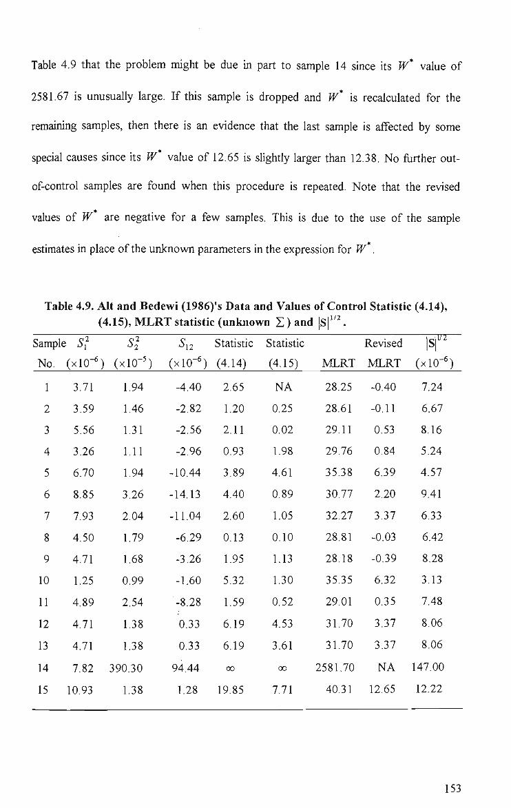
Table 4.9 that the problem might be due in part to sample 14 since its W* value of
2581.67 is unusually large. If this sample is dropped and W* is recalculated for the
remaining samples, then there is an evidence that the last sample is affected by some
special causes since its W* value of 12.65 is slightly larger than 12.38. No fiirther out-
of-control samples are found when this procedure is repeated. Note that the revised
values of W are negative for a few samples. This is due to the use of the sample
estimates in place of the unknown parameters in the expression for W*.
Table 4.9. Alt and Bedewi (1986)'s Data and Values of Control Statistic (4.14), (4.15), MLRT statistic (unknown Z ) and IS | l /2
Sampl(
No.
1
2
3
4
5
6
7
8
9
10
11
12
13
14
15
^ i3i
(xlO-^)
3.71
3.59
5.56
3.26
6.70
8.85
7.93
4.50
4.71
1.25
4.89
4.71
4.71
7,82
10.93
S'2
(xlO-^)
1.94
1.46
1.31
1.11
1.94
3.26
2.04
1.79
1.68
0.99
2.54
1.38
1.38
390.30
1.38
" 12
(xlO-^)
-4.40
-2.82
-2.56
-2.96
-10.44
-14.13
-11.04
-6.29
-3.26
-1.60
-8.28
0.33
0.33
94.44
1.28
Statistic
(4.14)
2.65
1.20
2.11
0.93
3.89
4.40
2.60
0.13
1.95
5.32
1.59
6.19
6.19
0 0
19.85
Statistic
(4.15)
NA
0.25
0.02
1.98
4.61
0.89
1.05
0.10
1.13
1.30
0.52
4.53
3.61
0 0
7.71
MLRT
28.25
28.61
29.11
29.76
35.38
30.77
32.27
28.81
28.18
35.35
29.01
31.70
31.70
2581.70
40.31
Revised
MLRT
-0.40
-0.11
0.53
0.84
6.39
2.20
3.37
-0.03
-0.39
6.32
0.35
3.37
3.37
NA
12.65
1 11 2
(xlO"^)
7.24
6.67
8.16
5.24
4.57
9.41
6.33
6.42
8.28
3.13
7.48
8.06
8.06
147.00
12.22
153

VO
>n
m
CN
ON
OO
t—
VO
m
CO
(N
I 00 13
on
CC
E O)
c o c i^ CO
D jw
co" 00
5
TJ c CC
Z Z
oe 03 01 0
CO
O
c o O c g
Q. «
b
"
\— LL
VO
i n
CO
CN
ON
OO a. i
X)
00 NO
V-)
CO
(N
oe oz 01 0
CO
E O)
CO c o c
J^ c ID d" fo G JW
CD~ CX) 05
0) T3 CU
C Q T5 C CO
CO JC O • Q
c o O c o
•{2 0 Q. CO
CD
L-
DpspBJS I0JJU03 opspBJS 10IIU03
154

4.7 Effect of Aggregation on Control Performance
As presented earlier, the proposed techniques involve the charting of some
aggregate-type statistics formed using independent components resulting from the
partitioning of the covariance matrices. Certainly, if the use of such a statistic incurs
some loss in control performance, then it is preferable to chart the individual components
separately though the improved performance is gained at the expense of increasing the
charting effort. In this section, the effect of such 'aggregation' on the control
performance, is briefly considered for the known Z case. This effect is examined by
comparing the probabilities of detection by the proposed technique with that based on
the use of the individual components for certain shifts in Z, having equated first their
false signal rates. Note that the latter technique, abbreviated hereafter as the IC
technique, involves the plotting of the following statistics :-
("^ - ^)Sx(k) (4.24)
^\
{n, r)SU...,-.(k) ^^2,...,/?. (4.25)
{n^-l)SlJd -e^.lr2p,id -e] (4.26) k l^''\~2(/fc) - 2 7 ' ' \-2(k) ~2J
and
(«. - sU.....,-J^^.^- e)' ^..^..,-ii^^^-i) J = X-,P (4.27)
It may also be of some value to study the control performance of the technique
based on the use of principal components. In the presence of Z, it is reasonable to chart
155
the standardized variances of the principal components (multiplied by (n-l) each)
separately. These are given by the diagonal elements of («-l)AoToSroA~o^ where AQ
and TQ denote respectively the diagonal matrix containing the eigenvalues of ZQ and
the matrix of the corresponding eigenvectors. For ease of subsequent discussion, this
technique is referred to as ISVPC.
Following a shift in the process covariance matrix Z, the statistics (4.24) and
(4.25) are readily seen to follow some scaled chi-square distribution whereas the
Hotelling X^-type statistics in (4.26) and (4.27) can be shown to be generally distributed
as linear combinations of independent noncentral chi-square variables (see A.ll).
Furthermore, note that the (conditional) independence of these statistics is preserved.
Thus, given the program of Davies (1980), it is possible to determine the overall
probability of 'picking up' any given shift in Z by the use of these statistics. However,
for mathematical convenience, only a special case is considered, namely, when the shifts
take the form :-
Zi = ^Zo>
a situation which has been noted earlier. Note that under these circumstances, all the
above statistics are chi-square except for the scalar multiple X. The same is true for the
ISVPC technique. Thus, the statistical performance of these and the proposed technique
depends on A, (besides/? and n) irrespective of ZQ •
For reasonable comparison, suppose that the significance levels associated with
the control charts for the IC and ISVPC techniques are set to be equal to a so that the
overall false signal rate, a, for each control scheme is the same as that of the proposed
technique. Accordingly, the a* for both techniques are respectively given by
156
I
a = l - ( l - a ) ' ' ' - ' and a = l - ( l - a ) ^
Furthermore, both the lower and upper control limits are used with each chart and these
* * OC ct
are set at — and 1 - — probability levels respectively. Note that under this condition,
the former technique is equivalent to Tippett's combination procedure as considered
earlier. The power of these and the proposed technique are given to 4 decimal places in
Table 4.10 for various combinations of/?, n, X and a. Note that the results for the
proposed technique are obtained by means of 5000 simulation runs. Note also the
proximity of the exact probabilities and the corresponding simulation resuhs for the IC
technique as given in Tables 4.3, 4.4 and 4.5. In all these cases, it is observed that the
proposed technique is significantly better than the IC and ISVPC techniques. It is also
seen that ISVPC ranks between the proposed and the IC technique in performance for all
the given shifts. Although no attempt has been made to study their relative performance
thoroughly, the results provide an indication that incorporating the individual
components into a composite statistic in the suggested manner may well result in
improved control performance.
157
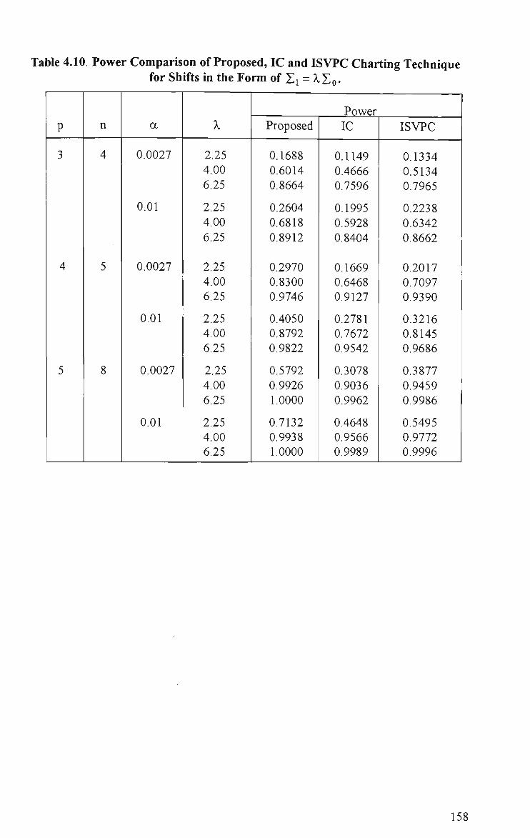
Table 4.10 Power Comparison of Proposed, IC and ISVPC Charting Technique for Shifts in the Form of Zi = >-Zo-
p
3
4
5
n
4
5
8
a
0.0027
0.01
0.0027
0.01
0.0027
0.01
X
2.25 4.00 6.25
2.25
4.00
6.25
2.25 4.00 6.25
2.25 4.00 6.25
2.25 4.00 6.25
2.25 4.00 6.25
Power Proposed
0.1688 0.6014 0.8664
0.2604 0.6818
0.8912
0.2970 0.8300 0.9746
0.4050 0.8792 0.9822
0.5792 0.9926 1.0000
0.7132 0.9938 1.0000
IC
0.1149 0.4666 0.7596
0.1995 0.5928 0.8404
0.1669 0.6468 0.9127
0.2781 0.7672 0.9542
0.3078 0.9036 0.9962
0.4648 0.9566 0.9989
ISVPC
0.1334 0.5134 0.7965
0.2238
0.6342 0.8662
0.2017 0.7097 0.9390
0.3216 0.8145 0.9686
0.3877 0.9459 0.9986
0.5495 0.9772 0.9996
158
CHAPTER 5
CAPABILITY INDICES FOR MULTIVARIATE
PROCESSES 1
5.1 Introduction
Since the pioneering work of Kane (1986), there have been many articles
published dealing with process capability indices. Some developments in process
capability analysis are outlined by Rodriguez (1992) in a special issue of the Journal of
Quality Technology, entirely devoted to the topic. In Marcucci and Beazley (1988), it
was noted that 'an index for multidimensional situations is another outstanding
problem '. Most of the relevant work to date has focussed on the developments of
process capability indices for single product characteristics. In many manufacturing
situations, the quality of a manufactured product is more often than not determined by
reference to more than one product characteristic. Invariably manufacturing conditions
are such that there is an inter-dependency in the development of these product
characteristics. To discuss process capability under these circumstances then, requires a
method that acknowledges this inter-dependency and constructs an index that
incorporates knowledge of the covariance structure of the quality characteristics.
The most commonly used univariate capability indices are the Cp, Cp^. and Cp^
indices which are defined as :-
r -U-L
^ This chapter is based on the paper entitled 'Capabilitity Indices for Multivariate Processes', Technical Report 49 EQRM14, Department of Computer and Mathematical Sciences, Victoria University of Technology, December 1994.
159

and Cp^ = 6Va'+(p-T)2
where p , a, U, L and T = - ^ denote the process mean, standard deviation, upper
and lower specification limits, and target respectively. The first is strictly concerned with
process potential in that it makes no reference to the process mean, p . However, they all
essentially reflect process potential in that they implicitly assume a perfectly controlled
process. For meaningfiil use of these indices to describe actual process behaviour
consideration of their sampling distributions is necessary. Statistical issues of estimation
and hypothesis testing and practical matters such as the use and interpretation of these
indices have been extensively discussed in the literature (see for eg., Kushler and Hurley
(1992), Franklin and Wasserman (1992), Peam, Kotz and Johnson (1992), Bamett
(1990) and Boyles (1991)). These indices are applicable for situations involving two-
sided specifications but some adaptations for one-sided specifications can also be found
in the literature.
After reviewing existing work on multivariate process capability indices, this
chapter explores fiirther the possibility of assessing multivariate process performance by
using a single composite measure and describes three approaches for doing so. In
particular, three bivariate process capability indices are proposed and some simple rules
provided for interpreting the values they take. The relative effectiveness of the proposed
indices as a comprehensive summary of process performance, with respect to all of the
measured characteristics, is also provided. An approximate test for one of the proposed
indices is developed. Possible methods of developing robust capability indices are also
considered. The paper focuses on the commonly encountered situations in which the
160

measured characteristics of a process or a product have two-sided specifications forming
a rectagular specification region. The extension of this work to situations involving
unilateral or a mixture of unilateral and bilateral tolerances is a straightforward matter.
The total discourse is given in the context of discrete item manufacturing.
5.2 A Review of Multivariate Capability Indices
Chan, Cheng and Spiring (1991) introduced a so-called multivariate version of
the Cp,„ index which is defined as :
C - ' "^ P^ \ n
Z(X,-T)^A-HX,-T) /=i
To do this, they made the assumption that the specification requirements for a v-variate
process or product are prescribed in the form of an ellipsoidal region given by
(X-T)^A"^(X-T)<c^
where X, T, A and C are respectively the v-dimensional random observation vector,
some specified v x 1 vector, a v x v positive definite matrix and a constant. These may
either be the actual engineering requirements or that created from various forms of
specifications in the suggested manner. For the latter case, it generally imposes more
stringent requirements than actually needed.
As the definition of Cp^ involves the sample observations rather than being based
on the process parameters (i.e the mean vector )LI and the covariance matrix Z), Pearn
et al.(1992) stated, quite correctly, that it should be taken as an estimator (denoted C „
) of the following revised index :
161
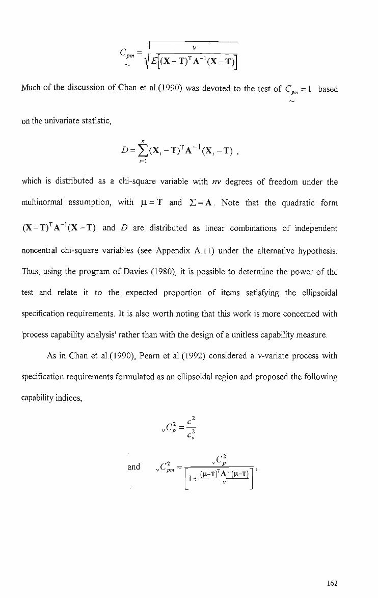
^pm £[(X-T)'^A-'(X-T)]
Much of the discussion of Chan et al.(1990) was devoted to the test of C „ = 1 based
on the univariate statistic,
Z) = X(X,-T)'^A-^(X,-T), ;=1
which is distributed as a chi-square variable with nv degrees of freedom under the
multinormal assumption, with |Ll = T and Z = A. Note that the quadratic form
(X-T) A" (X-T) and D are distributed as linear combinations of independent
noncentral chi-square variables (see Appendix A.ll) under the alternative hypothesis.
Thus, using the program of Davies (1980), it is possible to determine the power of the
test and relate it to the expected proportion of items satisfying the ellipsoidal
specification requirements. It is also worth noting that this work is more concerned with
'process capability analysis' rather than with the design of a unitless capability measure.
As in Chan et al.(1990), Pearn et al.(1992) considered a v-variate process with
specification requirements formulated as an ellipsoidal region and proposed the following
capability indices,
and
v^p
C^ =-V ^ pm
A r 1 (H-Tf A-'c^-T)!
J
162
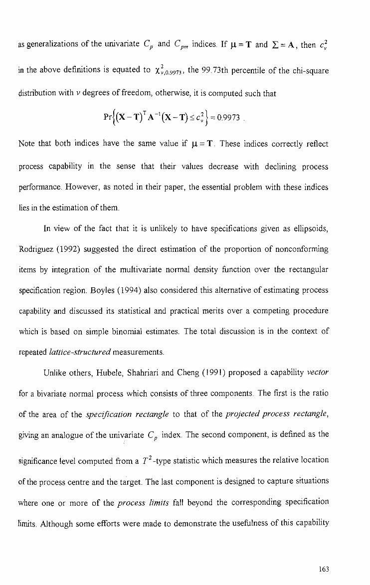
as generalizations of the univariate Cp and Cp„ mdices. If (i = T and Z = A, then cj
in the above definitions is equated to xl,0.9913, the 99.73th percentile of the chi-square
distribution with v degrees of freedom, otherwise, it is computed such that
Pr|(X-T)'^A"^(X-T)<c; I = 0.9973 .
Note that both indices have the same value if jLl = T. These indices correctly reflect
process capability in the sense that their values decrease with declining process
performance. However, as noted in their paper, the essential problem with these indices
lies in the estimation of them.
In view of the fact that it is unlikely to have specifications given as ellipsoids,
Rodriguez (1992) suggested the direct estimation of the proportion of nonconforming
items by integration of the multivariate normal density fiinction over the rectangular
specification region. Boyles (1994) also considered this alternative of estimating process
capability and discussed its statistical and practical merits over a competing procedure
which is based on simple binomial estimates. The total discussion is in the context of
repeated lattice-structured measurements.
Unlike others, Hubele, Shahriari and Cheng (1991) proposed a capability vector
for a bivariate normal process which consists of three components. The first is the ratio
of the area of the specification rectangle to that of the projected process rectangle,
giving an analogue of the univariate Cp index. The second component, is defined as the
significance level computed from a T^-type statistic which measures the relative location
of the process centre and the target. The last component is designed to capture situations
where one or more of the process limits fall beyond the corresponding specification
limits. Although some efforts were made to demonstrate the usefiilness of this capability
163

vector as a summary measure of the process performance, interpretation is sometimes
difficult.
Other contributions come from Taam, Subbaiah and Liddy (1993) who proposed
a multivariate capability index defined as
MC - ^o^^"^6 of-^1 '"" Volume of i?2
where R^ and i?2 represent respectively the modified tolerance region (modified
according to the process distribution) and the scaled 99.73% process region (scaled by
the mean squared error, Z j = [(X - T)(X - T)^l). If the process follows a multivariate
normal distribution, then the modified tolerance region here is the largest ellipsoid
inscribing the original specification region and the scaled process region, R2, is an
ellipsoidal region represented by (X - p,)^ Zj^ (X - (i) < xl,0.9973 • Thus, under normality
assumptions, this index becomes
Vol.(i?3) [i + (^_T)Tz- ' ( ^ -T) ]
^MCp
where Rj is the natural process ellipsoid containing 99.73% of items, MCp = voir ') is
an analogue of the univariate Cp (squared) index which measures the process potential
and Dj = 1 + ( J L I - T ) ^ Z " H M ' ~ T ) is a measure of process mean deviation from target.
As stated by Taam et al.(1993), this is an analogue of the univariate Cp^ (squared)
index. Note also that this index is similar to ^ Cp^, except in the marmer in which the
process potential and the deviation of mean from target are quantified. In terms of its
ease of computation and general applicability, it is superior to the latter. Besides the fact
164

that it can be used for different types of specification region (see the example on
geometric dimensioning and tolerancing (GDT) in the same paper), this index can be
extended to non-normal processes provided the specifications are two-sided. This,
however, entails the determination of the proper process and modified tolerance region
and the resuhing computations are likely to be complex. In the same paper, Taam et
al.(1993) considered the estimation of this capability index. However, they simply
replace the unknown mean vector |Ll and the covariance matrix Z in the expression for
the proposed index with the usual unbiased estimates and use Xv,o.9973 s the boundary of
the process ellipsoid without taking into consideration issues such as unbiasedness,
efficiency and uncertainty of the resulting capability index estimate. They also highlighted
some similarities and differences between the proposed index {MCp„), Cp^ and the
bivariate capability vector proposed by Hubele et al.(1991). A major problem with this
index is its potential to provide misleading conclusions. For instance, if the measured
characteristics are not independent and the index value is 1 (as a result of the process
being on-target and the volume of the process ellipsoid being the same as that of the
modified tolerance region), there is no assurance that the process under consideration is
capable of meeting the specifications consistently or can be expected to produce 99.73%
of conforming items. This is in conflict with the statement made by Taam et al.(1993)
that, ' when the process is centered at the target and the capability index is 1, it
indicates 99.73% of the process values he inside the tolerance region.' The deficiency in
this comment is illustrated in Figure 5.1 for a bivariate normal process.
165
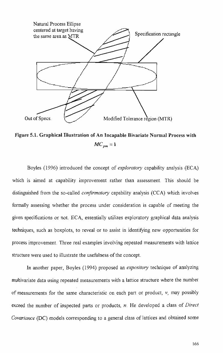
Natural Process Ellipse centered at target having the same area as Specification rectangle
Out of Specs. Modified Tolerance region (MTR)
Figure 5.1. Graphical Illustration of An Incapable Bivariate Normal Process with
MCp^ = 1
Boyles (1996) introduced the concept of exploratory capability analysis (ECA)
which is aimed at capability improvement rather than assessment. This should be
distinguished from the so-called confirmatory capability analysis (CCA) which involves
formally assessing whether the process under consideration is capable of meeting the
given specifications or not. ECA, essentially utilizes exploratory graphical data analysis
techniques, such as boxplots, to reveal or to assist in identifying new opportunities for
process improvement. Three real examples involving repeated measurements with lattice
structure were used to illustrate the usefulness of the concept.
In another paper, Boyles (1994) proposed an expository technique of analyzing
muhivariate data using repeated measurements with a lattice structure where the number
of measurements for the same characteristic on each part or product, v, may possibly
exceed the number of inspected parts or products, n. He developed a class of Direct
Covariance (DC) models cortesponding to a general class of lattices and obtained some
166

positive definite estimates of the covariance matrix denoted by Zp^ even when n<v.
This property of positive definiteness for the estimated covariance matrix permits the
computations of multivariate capability indices and estimated process yields which
depend on Z~^ when « < v or when n is not much greater than v, in which case the
usual sample covariance is ill-conditioned with respect to matrix inversion. He made
some efforts to justify the use of the proposed model for process capability analysis. In
particular, he demonstrated the superiority of employing Zj ^ to provide an estimate of
the proportion of nonconforming units over the use of sample covariance and the
empirical approach of simple binomial estimates. To do this he used sets of data from
Boyles (1996) along with some simulation results.
5.3 Constructing A Multivariate Capabilitv Index
With the assumption that the process under focus follows a multivariate normal
distribution, consider the following approaches to the design of a muhivariate process
capability index. Before proceeding, it should be pointed out that, although these
approaches have been widely discussed in simuhaneous interval estimation problems
(see, for example, Johnson et al. (1988) and Nickerson (1994)), they are used here in a
different context.
The first approach entails the construction of a conservative /?-dimensional
process rectangle from the projection of an exact ellipsoid (ellipse if bivariate) containing
a specified proportion of items on to its component axes. The edges of the resulting
process rectangle (the process limits) are then compared with their corresponding
specification limits. The associated index is defined in such a way that it is 1 if the
process rectangle is contained within the /?-dimensional specification rectangle with at
167

least one edge coinciding with its cortesponding upper or lower specification limits,
greater than 1 if the process rectangle is completely contained within the specification
rectangle and less than 1 otherwise. A bivariate capability mdex developed using this
approach is presented in the next section.
The second approach is based on the well known Bonferroni inequality. Unlike
the first one, this approach actually requires only the weaker assumption of normahty for
each individual product characteristic. The capability index using this approach is defined
in the same manner as above. The resulting process rectangular region having at least a
specified proportion of conforming items is compared with the specification rectangle.
The value of the proposed capability index reflects conservatively the process capability
of meeting the specifications consistently. In fact, the assessment of process performance
based on the Bonferroni inequality has been perceived by Boyles (1994) but it is used in
a different way and context. It should also be pointed out, despite his statement to the
contrary, that the given inequality
where
1-TZ = FT[-DI<XJ<D,, l<j<p\li,l) ,
l-TT, =Pr(x^. > - A , I<y</7 |H ,Z) ,
l -7r„=Pr(^, .<Z)„, l<7</? |H,Z) ,
is not generally true.
Another approach utilizes the multivariate normal probability inequality given by
Sidak (1967). It will be seen later, that a capability index constructed based on this
168

inequality and using arguments similar to the above, provides the best measure among all
those proposed in this paper.
5.4 Three Bivariate Capabilitv Indices
Suppose that the vector of the/? product characteristics, X = (Xi,X2,...,Xp]
follows a multivariate normal distribution with mean vector \i = ([i^,[i2,...,[Xp) and
covariance matrix Z . Further, suppose that a manufactured product is considered usable
if all its measured product characteristics are within their corresponding specification
limits i.e Lj < Xj <'Uj for j = l,...,p. Let 5 denote the proportion of unusable items
produced that can be tolerated. Our aim is to obtain the relationship between the
component means, the elements of the covariance matrix, 6 and the specification Umits
of all the measured characteristics by solving the following integral equation :
j ••• J j/(^l'^2---.^p)-^A2-"^p=l-5,
so that an index can be defined that reliably reflects the actual process capability. Directly
attempting to solve this equation is generally inadvisable due to computational
difficulties, so some approximations are presented.
169
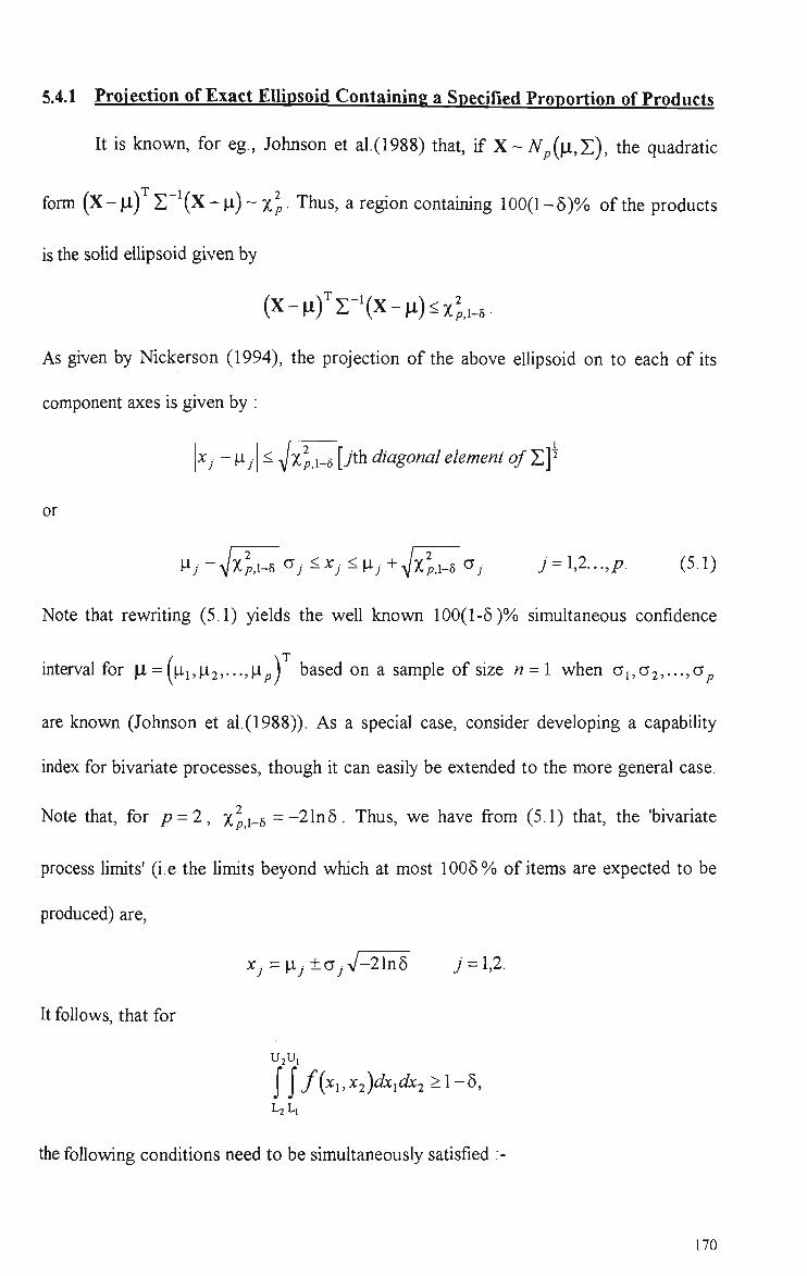
5.4.1 Projection of Exact Ellipsoid Containing a Specified Proportion of Products
It is known, for eg., Johnson et al.(1988) that, if X~Np(\i,T), the quadratic
form (X- |Ll) Z ' \ X - p) ~ xJ. Thus, a region containing 100(1-5)% of the products
is the soUd ellipsoid given by
(x-nfz-Xx-^)<xli-5.
As given by Nickerson (1994), the projection of the above ellipsoid on to each of its
component axes is given by :
Xj-[ij - V'^pj-s [yth diagonal element of Z]^
or
^j-^jy^^^^j^XJ<[iJ+^[xl^csJ 7 = 1,2...,/?. (5.1)
Note that rewriting (5.1) yields the well known 100(1-5)% simuhaneous confidence
interval for [i-\u.i,ii2,...,]ip] based on a sample of size n = l when ai,a2,...,a^
are known (Johnson et al.(1988)). As a special case, consider developing a capability
index for bivariate processes, though it can easily be extended to the more general case.
Note that, for p = 2, x^,i-8 =-2In5. Thus, we have from (5.1) that, the 'bivariate
process limits' (i.e the limits beyond which at most 1005% of items are expected to be
produced) are,
x^^p^. ±a^V-2ln5 j = l,2.
It follows, that for
U^Ui
l\f(xi,X2)dxidx2>l-^, L2L1
the following conditions need to be simuhaneously satisfied :-
170
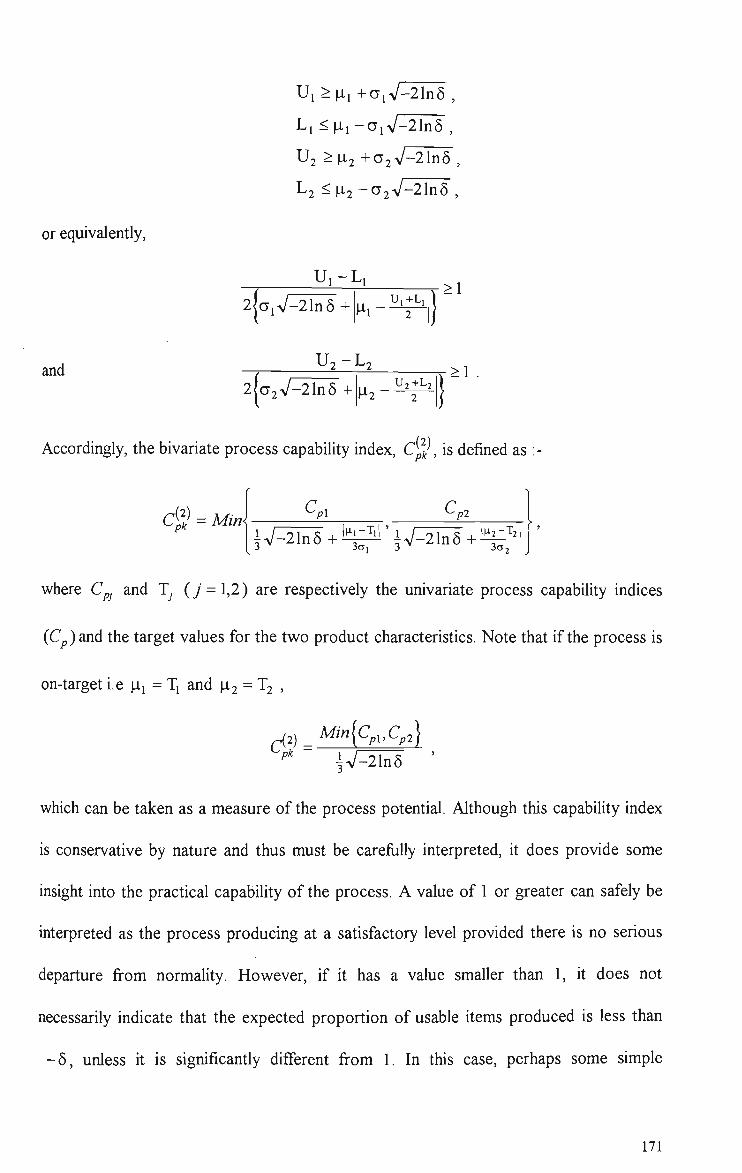
Ui>Pi+aiV-21n5 ,
Ll <Pi-aiV-21n5 ,
U2 >[i2+02^p2\nE,
Lj <P2 -cy2V-21n5 ,
or equivalently.
Ui -L i
l | o i V - 2 1 n 5 + | p i - ^ | | >1
and U2-L2
l |a2V-21n5+|p2--^^ |} >1
Accordingly, the bivariate process capability index, CyJ, is defined as
Cg = Mini C pi c p2
| V = 2 b 5 + 4 ^ ' i V = 2 b 6 + ^ 3c 3a,
where Cpj and Tj {j = 1,2) are respectively the univariate process capability indices
(C )and the target values for the two product characteristics. Note that if the process is
on-target i.e Pi = Tj and P2 = 2 ,
'-'pk _Min\Cp^Xp2[
V-21n5
which can be taken as a measure of the process potential. Although this capability index
is conservative by nature and thus must be carefijUy interpreted, it does provide some
insight into the practical capability of the process. A value of 1 or greater can safely be
interpreted as the process producing at a satisfactory level provided there is no serious
departure from normality. However, if it has a value smaller than 1, it does not
necessarily indicate that the expected proportion of usable items produced is less than
- 5 , unless it is significantly different from 1. In this case, perhaps some simple
171

guidelines or ad hoc rules would help to determine if the process capability is adequate.
Note the interesting fact that, although the covariance structure of the product
characteristics is considered in the development of the above, the proposed bivariate
capability index does not involve the correlation coefficient p of the two characteristics.
It is also noted that the proposed index has some similarity to the bivariate capability
vector proposed by Hubele et al.(1991). It differs from the latter, however, in that it
incorporates both the process potential and the deviation of the process mean from target
into a unitless measure. Hubele et al's capabihty index consists of three components, one
for measuring the process location, one for process dispersion (potential) and the other
for indicating whether any of the process limits is beyond its corresponding specification
limit(s). Whilst it may be argued that using separate indicators for each of the above
factors to reflect the process status may make the interpretation clearer, this process
capability vector involves more calculation and does not have any clear advantages over
the proposed index.
5.4.2 Bonferroni-Type Process Rectangular Re2ion
According to the Bonfertoni inequality, for a /?-variate process for which the
marginal distributions are normal, the p-dimensional centered process rectangle
containing at least 100(l -5 )% of items is given by :
p — z^o < Xj < ]ij + z^Oj, j = 1,2, , /? .
where Zg/2„ denotes the upper 100(5/2/?)th percentile of a standard normal
distribution. By replacing /? by 2 in the above, the bivariate process limits are obtained.
Proceeding as previously, another bivariate capability index is obtained and defined as.
172

'C^$ = Mm{ C pi c p2
i . .1 l>"i-Til ' 1 _ , h - T 2 | 3 ^ 8 / 4 ^ 3o, 3 ^ 5 / 4 + ^ ^ —
which has a similar interpretation. If /? = 1, 5 = 0.0027 and the process is on-target, this
type of multivariate capability index reduces to the univariate Cp, Cp,, and Cp„ indices.
It should be noted that this method of developing capability indices can be extended to
non-normal processes by replacing -Z5/4 and Z5/4 by the appropriate quantiles of the
process distribution.
5.4.3 Process Rectangular Region based on Sidak's Probability Inequality
As given by Sidak (1967), the multivariate normal probability inequality is :-
Pr ^> flTr{\z,\<c,] /=1
where Zj's are standard normal variables and c^'s denote some specified constants. For
Cj =c (/' = 1,2...,/?), this inequality becomes
Pr riKN' y=i
>[2<I>(c)-l]'
where 0(») denotes the cumulative distribution function of the standard normal variable.
Setting the lower bound, [20(c)-1]^ of the joint probability above, equal to - 6 ,
resuhs in a/?-dimensional process rectangle containing at least 100( -6 )% of items
given by :-
[ij - a , 0-'(i[i+(i-5)'''']) < Xj < j + a,4)-^(i[i+(i-5y''']), j = l,2,...,p,
173

where O ^(•) represents the inverse of the standard normal distribution fiinction. A
bivariate capability index is obtainable by replacing/? with 2 and comparing the resulting
bivariate process limits with the corresponding specification limits. This index is defined
as
^Cg = Mini ^p\ Cp2
[i<i.-'(i[i+vr5])+M'i<s-(i[uvr5]) So,
In the development of the above indices, it has been assumed that the tolerances
are bilateral and that the target or nominal specification is the midpoint of the
specification band, this, of course, is not always the case in practice. Under these
circumstances, redefinition of the indices using similar arguments is straightforward and
will not be discussed further.
As all of the above are of similar form, it is preferable to choose the one which is
least conservative or that best reflects the actual process capability. In the following
section, some comparisons between the three are provided in order to resolve this issue.
174

5.5 Some Comparisons of the Projected. Bonferroni and Sidak-tvpe Capabilitv Indices
Following conventional practice, the relative merits of the proposed capability
indices can be evaluated based on the following ratios :
_ Width of 100(1 - 5)% projected Interval for jth characteristic 1 "D.p — T T" ' ' '
Width of 100(1 - 5 j% Bonferroni Interval for jth characteristic
^ l l p , l -
^5/2/7
and
Width of 100(1 - 5)% projected Interval for jth characteristic •lSP ^^ / \
Width 0/100(1 - 5)% Sidak Interval for jth characteristic
ylx 2
P,i-5
<i,-i(i[i+(i_s)"^]) •
Note that the expressions for I^.p and I^.p remain the same irrespective of the product
characteristic being considered. One capability index is said to be less conservative than
the other if its construction is based on a shorter interval for the same 6 . Thus, according
to the definitions above, if Ig.p is greater than 1, the Bonferroni-type capability index is
better (less conservative) than that which is based on projections. Similarly, a value of
Isp greater than 1 implies that the Sidak-type index is superior to the projected one. As
for the relative effectiveness of the Bonferroni and Sidak-type indices, this is measured
by the relative magnitude of their corresponding I^.p and I^.p values. The values of
these indices are tabulated in Table 5.1 for some selected values of/? and 5 . It can be
seen from this table that, in all the reahstic cases considered, both the capability indices
based on the Bonfertoni and Sidak inequalities provide better measures than the
175

Projection-type capability index. The table also shows that, as the number of measured
characteristics, p increases, the better the Bonferroni or Sidak-type capabihty indices
become. Furthermore, as shown in the table, the Sidak-type capability mdex is marginally
better than that based on the Bonferroni inequality. The following section is devoted to
the development of a test concerning process capability based on the Sidak-type index.
Table 5.1. Relative Conservativeness of Projected, Bonferroni and Sidak-type Capability Indices.
p
2
3
5
10
5
0.0025 0.005 0.01 0.02 0.05
0.0025 0.005 0.01 0.02
0.05
0.0025 0.005 0.01 0.02 0.05
0.0025
0.005 0.01
0.02, 0.05
1.0726 1.0767 1.0811 1.0859 1.0921
1.1325 1.1397 1.1475 1.1561 1.1677
1.2319 1.2438 1.2569 1.2713 1.2917
1.4218
1.4419 1.4641 1.4886 1.5243
^^^ ~ cI,-'(i[l+(l-5)"''])
1.0727
1.0768 1.0815 1.0867 1.0945
1.1326 1.1398 1.1479 1.1570 1.1708
1.2320 1.2440 1.2574 1.2724 1.2953
1.4219
1.4421 1.4646 1.4899 1.5283
176
5.6 Testing the Capabilitv of a Bivariate Process
In practice, the assessment of process performance is often based on sample
estimates of some capability indices which are subject to uncertainty. Unless the sample
size is reasonably large, it is inappropriate to draw definite conclusions from these
process capability estimates. Of course, the need for process stability before computation
should also be emphasized, otherwise the interpretation of these indices is distorted,
regardless of how large the sample is. If meaningful interpretation of the estimated
capability is sought, it is important to take the sampling fluctuations of these estimates
into consideration. A common approach is to employ confidence mtervals. If point
estimates are to be used, it is desirable that estimation is unbiased and that the minimum
sample size required for an acceptable margin of estimation error is adhered to. Another
approach is based on testing hypotheses. Either approach generally requires knowledge
of the sampling distributions which are complicated. To circumvent this problem, we
develop an approximate test for the Sidak-type index C^C^^).
Consider the problem of testing the following hypotheses :
Under the null hypothesis, HQ , the process is capable and the worst scenario is when
both the Sidak-type process and specification rectangles coincide, in which case
^Cf^ = 1, On the other hand, the ahernative hypothesis, H^ corresponds to situations
where at least one edge of the process rectangle is beyond its corresponding specification
limit. The test proposed here is designed to capture such a situation.
A reasonable choice of the test statistic for this problem is.
177

'C^^,;=Min\ Ui-L, U 2 - L 2
2c5' i+2^1-Ti | '20^2+21^2-T2
where
c = <I>-'(i[l + V P 8 |
and, Xj and Sj denote respectively the mean and standard deviation of the jth product
characteristic based on a sample of size n. The decision rule is to reject HQ in favor of
Vf < k pk
where k is some positive constant depending on the significance level of the test (a) and
is determined from
MaxPrl^Cj^^ <k\HQistme| = a
The maximum value on the left-hand side of the above equation occurs when \Xj = T
and Uy -Ly =2caj for y = 1,2 (the worst situation under HQ). Thus, we have,
[ [c5i+|X,-^,|'c5'2+|X2-^2|J J
or
Pr n \{n-\)S] +
^r^i < n - l ."Y CTy c4n ylycsjl4n j ^
I = l - a (5.2)
According to the Bonferroni inequality.
Hn M
^ \ ' fOM)!^^
4~n- >l-XPr< 7=1
/«-! | ("- i )^; I 1 ^j-^j
cyfn \\aJl^fn > ^
(5.3)
178
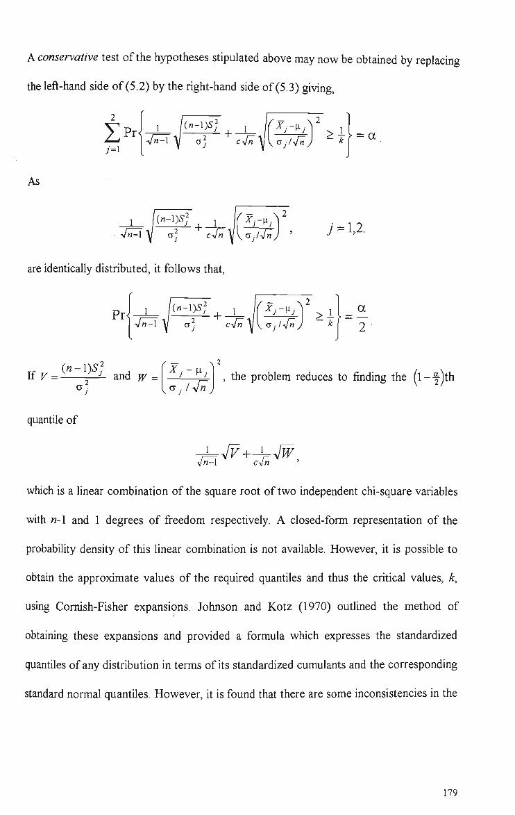
A conservative test of the hypotheses stipulated above may now be obtained by replacing
the left-hand side of (5.2) by the right-hand side of (5.3) giving,
2
/=1
L /("-^)-^7 I 1 h-\ c4n "Vv <Jjlyfn ^ >i^ = a
As
^ /("- ) > I 1 ir^ii^^"' / M - 1 CVM "y V <^ j i ^ y
7 = 1,2.
are identically distributed, it follows that.
Pr -hTA
\in-\)SJ ^ 1 ^ \ \ Ojl4n^ k{ 2
(n-l)S^ _, fx-a' If J/ = :: _LJ_ and W = —- ^ the problem reduces to finding the (l-^)th
quantile of
h-\ VF.
:Vn w
which is a linear combination of the square root of two independent chi-square variables
with n-l and 1 degrees of freedom respectively. A closed-form representation of the
probability density of this Unear combination is not available. However, it is possible to
obtain the approximate values of the required quantiles and thus the critical values, k,
using Cornish-Fisher expansions. Johnson and Kotz (1970) outlined the method of
obtaining these expansions and provided a formula which expresses the standardized
quantiles of any distribution in terms of its standardized cumulants and the corresponding
standard normal quantiles. However, it is found that there are some inconsistencies in the
179

results obtained by using the expression provided by these authors. As an ahernative,
numerical solutions are obtamed from the following integral equation :-
\FA{n-l)[llk-4^lc4^)%,{w)dw = l-^, 0 J 2
where /,(•) and F^(») respectively denote the probability density and the cumulative
distribution function of a chi-square variable with v degrees of freedom. The approximate
critical value, k, is obtained in this way using Mathematica version 2.2 (Wolfram (1991))
and given to 4 significant digits in Table 5.2 for various combinations of tolerable
proportion of unusable items (5 ), sample size («) and significance level (a).
Table 5.2. Critical Values for Testing " C ^
n
10
15
20
25
50
100
0.01
* 0.5763 t (0.5636)
0.6284 (0.6158) 0.6630 (0.6507)
0.6884 (0.6765) 0.7594 (0.7489) 0.8178
(0.8091)
a
0.025
0.6093 (0.5960) 0.6590 (0.6461) 0.6918 (0.6794)
0.7158 (0.7038) 0.7820 (0.7717) 0.8359 (0.8275)
0.05
0.6397 (0.6258) 0.6869 (0.6737) 0.7178 (0.7052) 0.7403 (0.7283) 0.8020 (0.7918) 0.8516 (0.8434)
0.1
0.6770 (0.6624) 0.7206 (0.7070) 0.7490 (0.7362)
0.7695 (0.7574) 0.8254 (0.8154) 0.8698 (0.8619)
* unbracketed values correspond to 5 = 0.01. t bracketed values correspond to 5 = 0.05.
180
5.7 Robustness to Departures From Normalitv — Some Considerations
Various attempts have been made to extend the definitions of the standard
univariate capability indices to situations where the process distribution is non-normal
and corresponding estimation procedures have been proposed. These are intended to
correctly reflect the proportion of items out of specification irrespective of the form of
the process distribution. No attempts have appeared in the literature, however, to
develop muhivariate capability indices which are insensitive to departures from
muhivariate normality. Some robust univariate capability indices and procedures for
assessing process performance currently available are briefly reviewed and an approach
ouflined for designing robust multivariate capability indices.
Chan, Cheng and Spiring (1988) suggested the use of a tolerance interval
approach to estimate, with a certain level of confidence, the interval within which at least
a specified proportion of items is contained. This estimated interval is then used in place
of the normal-theory based interval (some muhiple of a ) in the expressions for Cp, C j.
and Cp^. The 100(l-a)% confidence P -content tolerance interval is designed to capture
at least 1003% of the process distribution, 100(l-a)% of the time by using appropriate
order statistics. However, it was found by Chan et al. (1988) that the natural choice of
P, 0.9973 and a , 0.05, results in the requirement of taking sample sizes, n of 1000 or
larger. To circumvent this problem, they proposed the use of a tolerance interval with
smaller P, specifically, with P = 0.9546 and p = 0.6826 in place of 4a and 2a
respectively in the expressions for Cp, Cp^ and Cp^, and provided the corresponding
95% confidence estimators for sample sizes less than 300. Although this modification
181

greatly reduces the minimum sample size required, Peam et al. (1992) pointed out that 'it
depends on the (somewhat doubtful) assumption that the ratios of distribution-free
tolerance interval lengths for different P are always approximately the same as that for
normal tolerance intervals'. Furthermore, the proposed extensions retain the process
mean, p in the original definitions of C^ and Cp^ rather than replacing it by the
median. This complicates the interpretation of the resulting indices since the median may
differ considerably from the process mean for heavily skewed distributions.
Another approach to analysing process capability for non-normal processes
(especially unimodal and fairly smooth distributions) is based on systems or families of
distributions. Having redefined the standard Cp and C^ indices as
U - L P P _ P
-'0.99865 -MD.OOnS
and
Cpi, = Mini . [-^.99865 " M
= MJ "- 0 =
M-L 1 ^ ~M).00135j
^ 0 . 5 - L
1-^.99865 -^.5 -'O.S -^.00135.
where Pg denotes the 1005 th percentile of the distribution, Clement (1989) proposed
fitting a Pearson-type curve to the observed data using the method of moments and the
percentiles required for computation of these indices are then obtained from the fitted
distribution. The required standardized percentiles were tabulated for various
combinations of the coefficients of skewness and kurtosis. Some potential difficulties
with this approach were given by Rodriguez (1992). In view of the complexity and
difficulty of interpreting the equations for fitted Pearson and Johnson-type curves.
182

Rodriguez (1992) suggested the fitting of a particular parametric family of distributions
such as the Gamma, Lognormal or Weibull distribution to the process data. For checking
the adequacy of the distributional model, he recommended the use of statistical methods
based on the empirical distribution fiinction (EDF) including the Kolmogorov-Snumov
test, the Cramer Von Mises test and the Anderson-Dariing test. As for the graphical
checking of distributional adequacy, he stated that this can be accomplished by means of
quantile-quantile plots or probability plots. In the same paper, he also briefly described
the use of kernel density estimates for process capabihty analysis, especially for non-
normal distributions.
Pearn et al. (1992) suggested a possible approach to obtain a robust capability
index by defining an index
where 0 is chosen such that
PQ = P r [ p - e a < X < p + 0a] ,
is as insensitive as possible to the form of the distribution of X. He showed that, for
PQ = 0.99 the choice of 9 = 5.15 is quite adequate for a wide range of distributions.
For non-normal multivariate processes, it seems reasonable to use capability
indices constructed based on multivariate Chebyshev-type inequahties (see Johnson and
Kotz (1972), p.25) to reflect the process performance as no normality assumption is
required. The most basic type of these inequalities is obtained by combining the
Bonferroni and Chebyshev inequalities as follows :-
For our purpose here, the Bonferroni inequality is given by
183

" Q ^j-^j <k ) • > l - | ; p r {
;=1 '
Xj-^j >k] (5.4)
Upon applying the Chebyshev inequality to each term in the summation on the right-hand
side of (5.4), the following is obtained :-
Hn /= i
^r^j <k
.1-4 (5.5)
Note that, for the same k, the lower bound for (5.5) is smaller than that for (5.4).
However, this does not imply that the capability index constructed based on inequality
(5.5) is less conservative than that which is based on (5.4). For the same lower bound, 1-
6, the process rectangle based on the multivariate Chebyshev-type inequality (5.5) is
always larger (as a resuh of larger k) than that of (5.4) irrespective of the underlying
distribution. Note, however, that the Bonferroni-type capability index proposed in this
chapter is obtained by imposing a normality condition on the marginal distributions of the
process and thus it can be either too liberal or too stringent as a performance measure for
non-normal processes. For instance, a value greater than 1 for this index does not
guarantee that the expected proportion of non-defective items is more than 1-5 if the
process distribution is heavy-tailed (such as a muhivariate-? distribution) unless it is
significantly different from 1.
There are some improvements to the above muhivariate Chebyshev-type
inequality, however, the expressions involved are complicated, causing the construction
of multivariate capability indices based on them to be difficult except for situations where
there are relatively few variables. It is also found that these capability indices are only
184

margmally better than that based on inequality (5.5). Thus, h is reasonable to use (5.5)
whenever the use of distribution-free capability indices is wartanted.
185

CHAPTER 6
A COMPARISON OF MEAN AND RANGE CHARTS
WITH THE METHOD OF PRE-CONTROL i
6.1 Introduction
In 1924 Dr. Waher Shewhart first introduced the X and R charting technique
for the statistical monitoring and control of industrial processes. Now, after many
decades of use, they have become the core around which has been buih a body of
statistical techniques expressly designed for the purpose of controlling the quality of
manufactured products.
A competing procedure, employing a different strategy and known as 'pre-
control' (p.c), was proposed by Shainin (1954) as a replacement for various special
purpose plans for quality control and, in particular, as an improvement to the then 30
year old technique of X and R control. 'Pre-control' focuses directly on preventing non
conforming units from occurring, rather than on maintaining a process in a state of
statistical control, which is the strategy underpinning the use of X and R charts.
When assessing the merits and shortcomings of competing industrial control
procedures, the issue of statistical efficiency and more practical matters such as cost
effectiveness, extent and ease of use should all be considered. In fact these factors, to
varying degrees, play major roles in determining the overall success of quality
monitoring, maintenance and improvement efforts.
' This chapter is based on the paper entitled 'A comparison of mean and range charts with pre-control having particular reference to short-run production', Quality and Reliability Engineering International, Vol. 10, pp.477-485,1994.
186
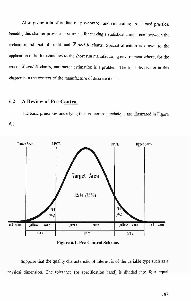
After giving a brief outhne of 'pre-control' and re-kerating hs claimed practical
benefits, this chapter provides a rationale for making a statistical comparison between the
technique and that of traditional X and R charts. Special attention is drawn to the
application of both techniques to the short run manufacturing environment where, for the
use of X and R charts, parameter estimation is a problem. The total discussion in this
chapter is in the context of the manufacture of discrete items.
6.2 A Review of Pre-Control
The basic principles underlying the 'pre-control' technique are illustrated in Figure
6.1.
Lower
red zone
Spec. LP
^ ^ ^ (7%)
yellow zone
1/4 X
CL
^ Target Area ^
12/14 (86%)
UP
green zone
\ii\
CL Upper
yellow zone
1/4 X
spec.
red zone
Figure 6.1. Pre-Control Scheme.
Suppose that the quality characteristic of interest is of the variable type such as a
physical dimension. The tolerance (or specification band) is divided into four equal
187

sections and the boundaries of the outer two are called 'pre-control' Unes. The area
between these lines is described as the 'target area' or the green zone. The remaining
areas between the two specification limits, L and U, are labelled the yellow zones and
those beyond the specification hmits, the red zones. Assuming that the measurements on
the product characteristic are normally distributed, correctly centered and that the
process is just capable of meeting the specifications, then approximately 1 in 14 times an
observation will fall in either yellow zone by chance alone. A barely capable process is
one having Cp = 1 where Cp={U-L)l6a, a being the process standard deviation. A
single observation falling in these zones is not deemed an indication of the presence of a
process disruption. Two consecutive values in these zones, however, or one in the red
zone, is considered adequate evidence of trouble and grounds for process adjustment.
'Pre-Control' operating rules are developed around these fiindamental notions. In
a slightly different version (Bhote (1980) and Logothetis (1990)), the decision for
approval of set-up and resumption of a corrected process is based on the following rule :
'... If five consecutive units are within the target area before the occurrence
of a red or a yellow, the set-up is qualified and full production can begin ...'.
The reason is that this occurrence indicates that the process is well centered and highly
likely to be producing at a satisfactory quality level. The probabiUties of approving a set
up which is centered at the nominal dimension, for various process capabilities, C , and
using the above rule, are given in Table 6.1.
Table 6.1. Probability of Set-up Approval for Pre-Control
Cp
Prob.
0.50
0.0489
0.75
0.2210
1.00
0.4882
1.25
0.7308
1.33
0.7919
1.50
0.8838
188

If five consecutive greens prove difBcuh to obtain, then this is an indication that
the process is either incorrectly centered and requires adjustment, or that the process is
not capable of consistently meeting the specifications. This check rule is useful for short
production runs for which the 'set-up' is a crucial factor affecting the quality of the
subsequent process output.
Once the process has passed the initial set-up stage, periodically two
consecutively produced items are examined to monitor performance. Having hems in
either of the yellow zones is acceptable, except when two occur consecutively. Two
successive yellows on the same side of the target, signal the departure of the process
mean from the target value. If they occur on different sides of the target, the process
spread has most likely increased beyond its acceptable limit. In this manner, 'pre-control'
enables corrective action to be taken usually before unacceptable work is produced and,
hopefully, avoids repeated minor, and unnecessary cortections. In the event of getting an
item in either part of the red zone, the process is stopped immediately, as h is already
producing defectives. Variations in this 'pre-control' plan, apphcable to less common
situations are given by Shainin (1954) and Putnam (1962).
In order to justify his recommendation for 'pre-control', Shainin (1965, 1984) made
some efforts to discuss its statistical power. These included consideration of the long run
expected proportion of nonconforming units produced resulting from the ongoing use of
'pre-control' based on a particular sampling rule. He showed that the maximum value of
this quality measure, termed the average produced quality limit (APQL), does not exceed
2% for normally distributed processes if 6 inspection checks, on average, are made
between typical process adjustments (Shainin (1984)). Some very general discussion
189

about the sampling frequency appeared in Satterthwahe (1973), Shainin (1990) and
Traver (1985). Without previous knowledge of the average time between process
adjustments, Shainin (1984) suggested that a 20-minute sampling interval should first be
used and adjusted subsequently.
As pointed out by Cook (1989), some of the expressed doubts about 'pre-
control' relate to the normality assumption. The general consensus amongst practitioners
is that even for stable processes it is doubtful that the fit to normality in the distribution
tails is particularly close. Sinibaldi (1985) used simulation techniques to examine the
effect of non-normality on the appropriateness of'pre-control'. In addition, he evaluated
the relative performance of 'pre-control' and X and R control on normal and skewed
distributed processes with frequently changing means. The resuhs of the comparison
indicate that X control causes fewer incorrect mean shift signals and has better control
to target (as measured by the overall average, X and the average distance of all hems
produced from the process target) than 'pre-control'. However, using the R chart to
detect deterioration in the process spread resuhs in more false alarms than using 'pre-
control' for the same purpose.
Bhote (1980) attempted to illustrate some 'weaknesses' in X and R control
charting, using two case studies. Taking a more complete view, Logothetis (1990)
argued effectively that, desphe its simplicity, 'pre-control' cannot be considered a serious
technique of statistical process control (SPC). He, in fact, used the same case studies as
Bhote (who used them to illustrate the 'weaknesses' of X and R control charts) to
demonstrate the usefulness of SPC as a whole and the weaknesses of 'pre-control'.
However, no comparison has been made between 'pre-control' and X and R charts on
the basis of average run length (ARL). This is due to the fact that, 'pre-control' lines are
190
derived from specification hmits, causing the ARL for a given mean shift to vary
according to the actual process capability (C^).
6.3 The Practical Merits of Pre-Control
There is little mention of 'pre-control' in many standard text books on statistical
process control, desphe h having certain practical advantages over X and R charts. This
could indicate a belief that a reasonable statistical comparison between the two
techniques is not legitimate, that there is a reluctance to forsake X and R charting since
the method has proven usefiil over many years and in many industries or indicate a view
aligned with that of Logothetis (1990) that 'pre-control' is too limited in hs perspective.
With the unique setup rule of 'pre-control', the first five consecutively
manufactured units are all that is required to determine whether any process-tolerance
incompatibilities exist before fiiU production is aUowed to commence. There is, of
course, no definite knowledge of how many units will have to be checked before five
consecutive good ones are obtained. In comparison, when using X and R charts, it is
necessary to have fairly long process trial runs in order to collect sufficient sample data
to establish the existence of a state of statistical control, and subsequently, to estimate
the process standard deviation so as to correctly locate the control lines.
Following setup approval, 'pre-control* provides for the occasional sampling of two
consecutively produced hems in order to monitor on-going process performance, in
contrast to the routine sample size of four or five often recommended for use of
X and R charts. No calculations need to be performed for 'pre-control' operation except
for the extremely simple initial setting of 'pre-control' lines, whereas continual routine
191

computations are involved whh use of X and R charts. For these latter, h is not only
necessary to calculate the control statistics for subgroups, but also necessary to estimate
and revise the control hmits from time to time.
For 'pre-control', measurements can be observed and compared to specification
limits in a way that is easily understood by operators whhout much likehhood of
misinterpretation. Additional worker participation in decision making and problem
solving may be gained through operators having a better appreciation of the techniques
in use.
Whilst, in practice, determination of the sampling interval for X and R charts is
arbitrary, 'pre-control' provides a simple and flexible rule of six inspection checks per
trouble indication which, on a long term basis, resuhs in a maximum average fraction
defective of less than 2% for a normally distributed process (Shainin (1984)). A
successful application of 'pre-control' in a 'zero defects' environment has been reported
by Brown (1966). Regulating sampling on the basis of recent process performance,
seems a more reasonable and efficient approach to adopt than sampling at fixed intervals,
as it entails more frequent sampling when the process is unsatisfactory.
Such eventualities as tool wear do not cause a premature reaction from 'pre-
control'. It will only issue warning signals at times when the process is soon likely to
produce defective products. What can be considered un-necessary process adjustments,
which have the potential to make production performance worse, are, therefore, avoided.
Since 'pre-control' does not require exact measurements but only needs to note
the zone into which the measurements fall, complex and expensive measuring equipment
may be replaced by 'go/no-go' colour coded gauges. Furthermore, electronic gauging can
192

be considerably simplified if it is only required to distinguish between a few measurement
bands. As a resuh, there can be a reduction in caphal investment and calibration costs
Another important feature of 'pre-control' is hs ready applicabihty to a variety of
situations including the short production run manufacturing environment which has
become increasingly prevalent following the general move into Just-In-Time (JIT)
production and flexible manufacturing.
Despite its many years of existence and its apparent practical merits, given in
brief here, 'pre-control' has not been widely adopted as a replacement for traditional
X and R charts. Logothetis (1990) extensively criticised adoption of'pre-control' over
the use of X and R charts on a number of grounds. It is intended that the material
contained in this chapter will provide some additional, statistically based arguments that
will help facihtate a rational judgement on which of the two techniques to adopt in any
given situation.
6.4 Short Runs and Pre-Control
There is no universally agreed definition of a 'short run', however, the term is
often used to describe production processes Avith typically fewer than 50 hems made
within a single machine set-up. Short runs, therefore, at a first glance, do not readily lend
themselves to the use of Shewhart X and R charts.
The essential problem that obstructs the apphcation of standard control charting
techniques in short production run situations is the inability to estimate the process
variability, because of insufficient data. The problem is fiirther aggravated by problems of
process 'warm up'. Using data from the 'warm up' period to obtain control limits can
193
lead to erroneous conclusions regarding past, current and future states of the process
(see Murtayetal.( 1988).
Unlike X and R charts, 'pre-control' is a control technique which predetermines
its control limits by reference to product specifications only, rather than requiring an
accumulation of data for computation of them. It is also capable of handling the problem
of process 'warm up'. It is, therefore, highly suitable for application to short production
runs.
6.5 A Statistical Comparison Between Pre-Control and X-bar and R Charts
For short production runs, when there is insufficient previous data available to
obtain the control limits for X and R charts, a number of authors (see, for example,
Sealy (1954) and Bayer (1957) have proposed setting control limits on the assumption
that the process is just capable of meeting specifications (i.e. C^ = 1) and assuming that
the mean level of the process is equal to the nominal or target value. This adaptation
provides a basis for a statistical comparison between 'pre-control' and X and R charts.
In the following comparison, a subgroup size of four is chosen for the application
of X and R charts because this is commonly recommended. It is also assumed that the
quality characteristic under consideration is normally distributed or approximately so and
that no supplementary run rules are used with the X chart. First, consider the
probabilhies of detection by the sample immediately following a process mean shift,
using an X chart and a 'pre-control' chart. These probabilities are provided in Tables 6.2
and 6.3 for various combinations of process capability (C^) and mean shifts in multiples
{k) of the standard deviation {a). In both tables, the entries are the probabilities of
194

issuing a cortect signal of the mean shift except when k = 0, in which case the values
tabulated are the probabilhies of a false warning. Signals from 'pre-control' that we
employ here as indication of a process mean shift, are 2 consecutive hems in the same
yellow zone, or 1 in the red zone and the other not faUing beyond the 'pre-control' line on
the opposhe side of the nominal value. Furthermore, h should be noted that the control
lunits for the X and R charts are set using conventional control chart factors with the
addhional assumptions that,
f/+Z ^ U-L u = and <j- .
2 6
The entries in Table 6.3, other than those corresponding to C = , are the probabilities
of detecting a mean shift of the indicated magnitudes when the C has been assumed 1
but is in fact the value indicated. It has been adequately demonstrated in the literature
that the X chart is tardy in registering small changes in the process mean. Where the
'speedy' detection of small mean shifts is required, addhional control rules or ahernative
charting techniques are necessary. Thus the tables provide, for comparison, probabilities
for a number of realistic mean shifts; realistic in the sense that they reflect situations
where X (with no additional rules) and 'pre-control' can conceivably be considered
competing techniques. Besides having a lower likelihood of a false signal, the X chart
possesses a higher probability of 'picking up' the mean shift irrespective of the actual
process capability, except where indicated by *, when the difference between
corresponding entries in the two tables is marginal. In one sense, a more reasonable
comparison can be accomplished through adjusting the control limits for the X chart in
such a way that the resulting probability of issuing a false signal, when C^ = 1, is the
same as that of'pre-control'. This involves moving the control lines nearer to the nominal
195

or target value. Following such a modification, the cortesponding probabihties of
immediate detection are given in Table 6.4. Tables 6.2 and 6.4 clearly illustrate the
superiority of the X chart in terms of senshivity to process mean shifts.
Table 6.2. Power of Pre-Control-Mean Shift
Cp \ k
0.50
0.75
1.00
1.25
1.33
1.50
0
0.2488
0.0701
0.0136
0.0022
0.0012
0.0003
±1.0
0.5814
0.3153
0.1264
0.0412
0.0279
0.0116
±1.5
0.8125
0.5759
0.3166
0.1410
0.1051
0.0534
±2.0
0.9418
0.8072
0.5759
0.3383
0.2752
0.1685
±2.5
0.9879
0.9391
0.8057
0.5950
0.5223
0.3767
Table 6.3. Power of X Chart with 3a Limits (assumed C = 1)
Cp \ k
0.50
0.75
1.00
1.25
1.33
1.50
0
0.1336
0.0244
0.0027
0.0002
0.0001
0.0000
±1.0
0.6915
0.4013
0.1587
0.0401*
0.0232*
0.0062*
±1.5
0.9332
0.7734
0.5000
0.2266
0.1611
0.0668
±2.0
0.9938
0.9599
0.8413
0.5987
0.5040
0.3085
±2.5
0.9998
0.9970
0.9773
0.8944
0.8438
0.6915
196
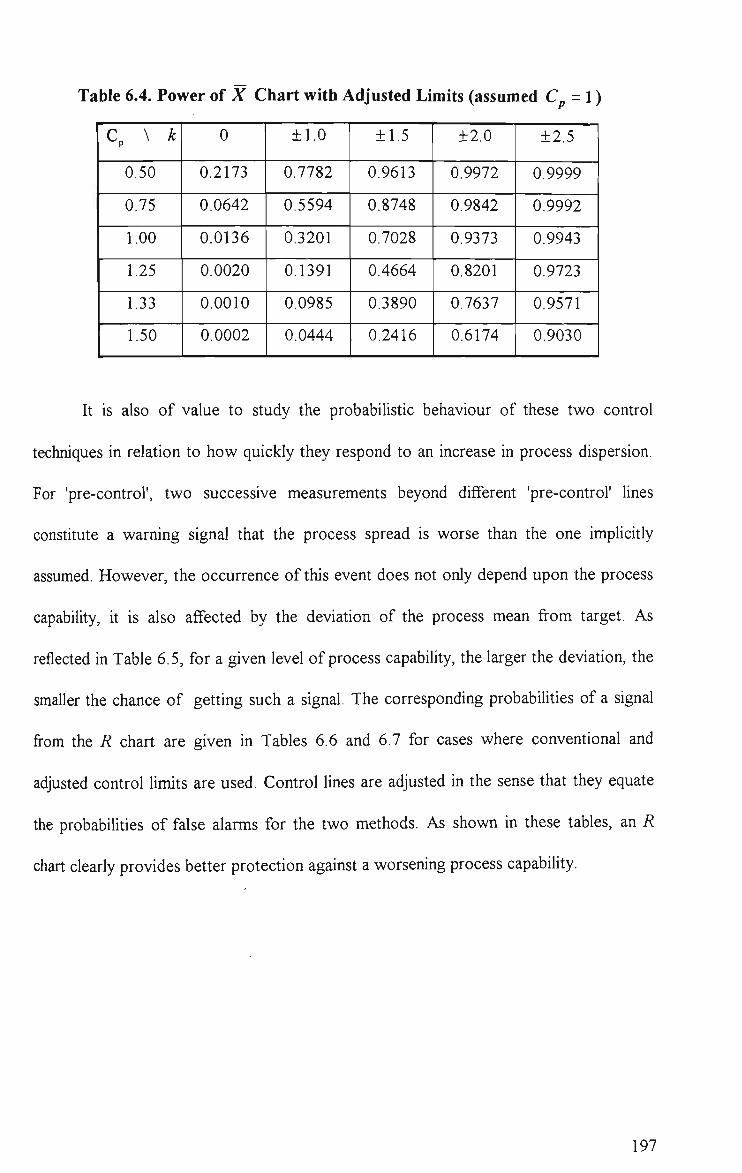
Table 6.4. Power of X Chart with Adjusted Limits (assumed C = 1)
Cp \ k
0.50
0.75
1.00
1.25
1.33
1.50
0
0.2173
0.0642
0.0136
0.0020
0.0010
0.0002
±1.0
0.7782
0.5594
0.3201
0.1391
0.0985
0.0444
±1.5
0.9613
0.8748
0.7028
0.4664
0.3890
0.2416
±2.0
0.9972
0.9842
0.9373
0,8201
0,7637
0.6174
±2.5
0.9999
0.9992
0.9943
0.9723
0.9571
0.9030
It is also of value to study the probabiUstic behaviour of these two control
techniques in relation to how quickly they respond to an increase in process dispersion.
For 'pre-control', two successive measurements beyond different 'pre-control' lines
consthute a warning signal that the process spread is worse than the one implichly
assumed. However, the occurrence of this event does not only depend upon the process
capability, h is also affected by the deviation of the process mean from target. As
reflected in Table 6.5, for a given level of process capability, the larger the deviation, the
smaller the chance of getting such a signal. The corresponding probabihties of a signal
from the R chart are given in Tables 6.6 and 6.7 for cases where conventional and
adjusted control limits are used. Control lines are adjusted in the sense that they equate
the probabilities of false alarms for the two methods. As shown in these tables, an R
chart clearly provides better protection against a worsening process capabihty.
197

Table 6.5. Power of Pre-Control - Increase in Dispersion
Cp \
0.50
0.65
0.75
0.85
1.00
0
0.1027
0.0543
0.0340
0.0205
0.0089
±1.0
0.0480
0.0246
0.0151
0.0090
0.0038
±1.5
0.0189
0.0093
0.0056
0.0033
0.0014
±2.0
0.0053
0.0025
0.0014
0.0008
0.0003
±2.5
0.0011
0.0005
0.0003
0.0001
0.0001
Table 6.6. Power of R Chart-Conventional Limits (assumed C„ = 1)
Cp
Prob.
0.50
0.3445
0.65
0.1349
0.75
0.0613
0.85
0.0246
1.00
0.0049
Table 6.7. Power ofR Chart-Ad justed Limits (assumed C = 1)
Cp
Prob.
0.50
0.3940
0.65
0.1715
0.75
0.0850
0.85
0.0376
1.00
0.0089
Tables 6.8 and 6.9 provide average run lengths for detection of a mean shift using 'pre-
control' and an X chart respectively, based on the probabihties contained in Tables 6.2
and 6.3.
198
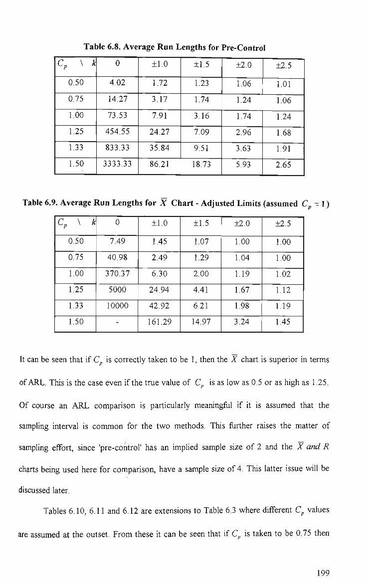
Table 6.8. Average Run Lengths for Pre-Control
Cp \ k
0.50
0.75
1.00
1.25
1.33
1.50
0
4.02
14.27
73.53
454.55
833.33
3333.33
±1.0
1.72
3.17
7.91
24.27
35.84
86.21
±1.5
1.23
1.74
3.16
7.09
9.51
18.73
±2.0
1.06
1.24
1.74
2.96
3.63
5.93
±2.5
1.01
1.06
1.24
1.68
1.91
2.65
Table 6.9. Average Run Lengths for X Chart - Adjusted Limits (assumed C- = 1)
Cp \ k
0.50
0.75
1.00
1.25
1.33
1.50
0
7.49
40.98
370.37
5000
10000
-
±1.0
1.45
2.49
6.30
24.94
42.92
161.29
±1.5
1.07
1.29
2.00
4.41
6.21
14.97
±2.0
1.00
1.04
1.19
1.67
1.98
3.24
±2.5
1.00
1.00
1.02
1.12
1.19
1.45
It can be seen that if Cp is correctly taken to be 1, then the X chart is superior in terms
of ARL. This is the case even if the true value of C is as low as 0.5 or as high as 1.25.
Of course an ARL comparison is particularly meaningfiil if h is assumed that the
sampling interval is common for the two methods. This fiirther raises the matter of
sampling effort, since 'pre-control' has an implied sample size of 2 and the X and R
charts being used here for comparison, have a sample size of 4. This latter issue will be
discussed later.
Tables 6.10, 6.11 and 6.12 are extensions to Table 6.3 where different C values
are assumed at the outset. From these h can be seen that if Cp is taken to be 0.75 then
199

there is little difference in the two methods even if the C value is in fact 0.5. 'Pre-
control' has less likelihood of false alarms, however. When Cp is assumed to be 1.25,
even if the actual value is as low as 0.5 or as high as 1.50 the X chart is superior for
detecting all the given mean shifts. Similarly for the assumption of Cp = 1.50, except
here, 'pre-control' is marginally superior with respect to false alarms. Tables 6.13 and
6.14 are similar extensions to Table 6.6.
Table 6.10. Power of X Chart (assumed C_ = 0.75)
Cp \ k
0.50
0.75
1.00
1.25
1.33
1.50
0
0.0455
0.0027
0.0001
0.0000
0.0000
0.0000
±1.0
0.5000
0.1587
0.0228
0.0014
0.0005
0.0000
±1.5
0.8413
0.5000
0.1587
0.0228
0.0102
0.0014
±2.0
0.9773
0.8413
0.5000
0.1587
0.0934
0.0228
±2.5
0.9987
0.9773
0.8413
0.5000
0.3745
0.1587
Table 6.11, Power of X Chart (assumed C_ = 1.25)
Cp \ k
0.50
0.75
1.00
1.25
1.33
1.50
0
0.2301
0.0719
0.0164
0.0027
0.0014
0.0003
±1.0
0.7881
0.5793
0.3446
0.1587
0.1166
0.0548
±1.5
0.9641
0.8849
0.7258
0.5000
0.4239
0.2743
±2.0
0.9974
0.9861
0.9452
0.8413
0.7905
0.6554
±2.5
0.9999
0.9993
0.9953
0.9773
0.9647
0.9192
200

Table 6.12. Power of X Chart (assumed C = 1.50)
Cp \ k
0.50
0.75
1.00
1.25
1.33
1.50
0
0.3173
0.1336
0.0455
0.0124
0.0078
0.0027
±1.0
0.8413
0.6915
0.5000
0.3085
0.2546
0.1587
±1.5
0.9773
0.9332
0.8413
0.6915
0.6331
0.5000
±2.0
0.9987
0.9938
0.9773
0.9332
0.9099
0.8413
±2.5
1.0000
0.9998
0.9987
0.9938
0.9904
0.9773
Table 6.13. Power of i? Chart (assumed C_ = 1.25)
Cp
Prob.
0.50
0.5445
0.65
0.3093
0.75
0.1904
0.85
0.1078
1.00
0.0393
1.25
0.0049
Table 6.14. Power of if Chart (assumed C_ = 1.50)
Cp
Prob.
0.50
0.6851
0.65
0.4745
0.75
0.3445
0.85
0.2355
1.00
0.1192
1.25
0.0289
1.50
0.0049
If the X and R charts are for use whh short production runs, it may not make a
great deal of sense to compare their effectiveness with 'pre-control' on the basis of
average run length. This is the case when the total production time is less than the time
taken to collect enough samples to match the ARL. As an alternative, we consider the
probability of detection whhin 5 successive samples following a given mean shift. This
probability is plotted against process mean shift in standard deviation units for 'pre-
control' and X charts with both conventional and adjusted control limits in figures 6.2(a)
to 6.2(f) where the X chart is constructed under the assumption that C is 1. As shown,
there is no remarkable difference between 'pre-control' and X charts whh either
201

conventional or adjusted control hmits if C^ = 0.5 or 0.75 . However, considerable
differences exist between these techniques if the process is more than capable, especially
for mean shifts ranging from la to 2a.
202
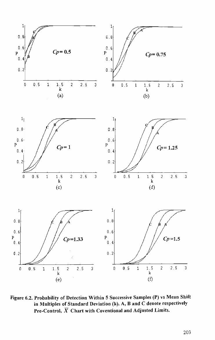
Cp= 0.5
0 0 .5 1 1 .5 2 2 .5 3 0 0.5 1 1.5 2 2 .5 3 k k
(a) (b)
(c) (d)
(e) (f)
Figure 6.2. Probability of Detection Within 5 Successive Samples (P) vs Mean Shift in Multiples of Standard Deviation (k). A, B and C denote respectively Pre-Control, X Chart with Coventional and Adjusted Limits.
203

6.6 Equating Sampling Effort
In our discussion so far, the total sampling effort has not been taken into
consideration; the assumption being made that the time and cost of sampling,
measurement or testing are not significant. This may, however, be unrealistic in certain
circumstances. If h is, no usefiil comparison can be made unless the relative sampling
frequency of'pre-control' and X and R control is first set in such a way that use of both
methods involves the same sampling effort.
To compensate for the smaller sample size of 2 for 'pre-control', we assume that
process checks are made twice as often as X andR control with a sample size of 4. This
being the case, we focus on the average number of items required to detect a change in
the process mean or process dispersion, using the two methods.
In Tables 6.15 and 6.16, the average number of units sampled before 'picking up'
various mean shifts under different process capability levels are given for 'pre-control'
and X chart control (control hnes fixed on the basis that C^ = 1). To facihtate the
comparison, we have computed the following index :
•ANIIMS(PC)
-'MS
ANII(X)
ANII(J)
if k ^ 0
if yt ^ 0 [ANII^s(PC)
where ANIIj^s(PC) and ANII(X) denote the average number of hems inspected before
detecting the mean shift using 'pre-control' and conventional X chart (control based on
Cp = l) respectively except when A: = 0, in which case they are the average number of
hems inspected prior to the occurrence of a false signal.
204
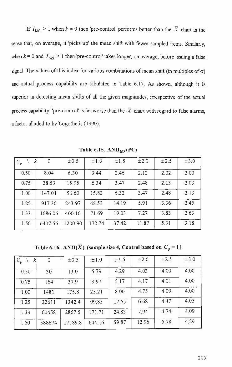
If /j^s > 1 when k^O then 'pre-control' performs better than the X chart in the
sense that, on average, h 'picks up' the mean shift with fewer sampled hems. Similariy,
whenk=0 and /^s > 1 then 'pre-control' takes longer, on average, before issuing a false
signal. The values of this index for various combinations of mean shift (in multiples of a)
and actual process capability are tabulated in Table 6.17. As shown, although h is
superior in detecting mean shifts of all the given magnitudes, irrespective of the actual
process capability, 'pre-control' is far worse than the X chart whh regard to false alarms,
a factor alluded to by Logothetis (1990).
Table 6.15. ANnMs(PC)
Cp \ k
0.50
0.75
1.00
1.25
1.33
1.50
0
8.04
28.53
147.01
917.36
1686.06
6407.56
±0.5
6.30
15.95
56.60
243.97
400.16
1200.90
±1.0
3.44
6.34
15.83
48.53
71.69
172.74
±1.5
2.46
3.47
6.32
14.19
19.03
37.42
±2.0
2.12
2.48
3.47
5.91
7.27
11.87
±2.5
2.02
2.13
2.48
3.36
3.83
5.31
±3.0
2.00
2.03
2.13
2.45
2.63
3.18
Table 6.16. ANn(Ar) (sample size 4, Control based on C = 1)
Cp \ k
0.50
0.75
1.00
1.25
1.33
1.50
0
30
164
1481
22611
60458
588674
±0.5
13.0
37.9
175.8
1342.4
2867.5
17189.8
±1.0
5.79
9.97
25.21
99.85
171.71
644.16
±1.5
4.29
5.17
8.00
17.65
24.83
59.87
±2.0
4.03
4.17
4.75
6.68
7.94
12.96
±2.5
4.00
4.01
4.09
4.47
4.74
5.78
±3.0
4.00
4.00
4.00
4.05
4.09
4.29
205
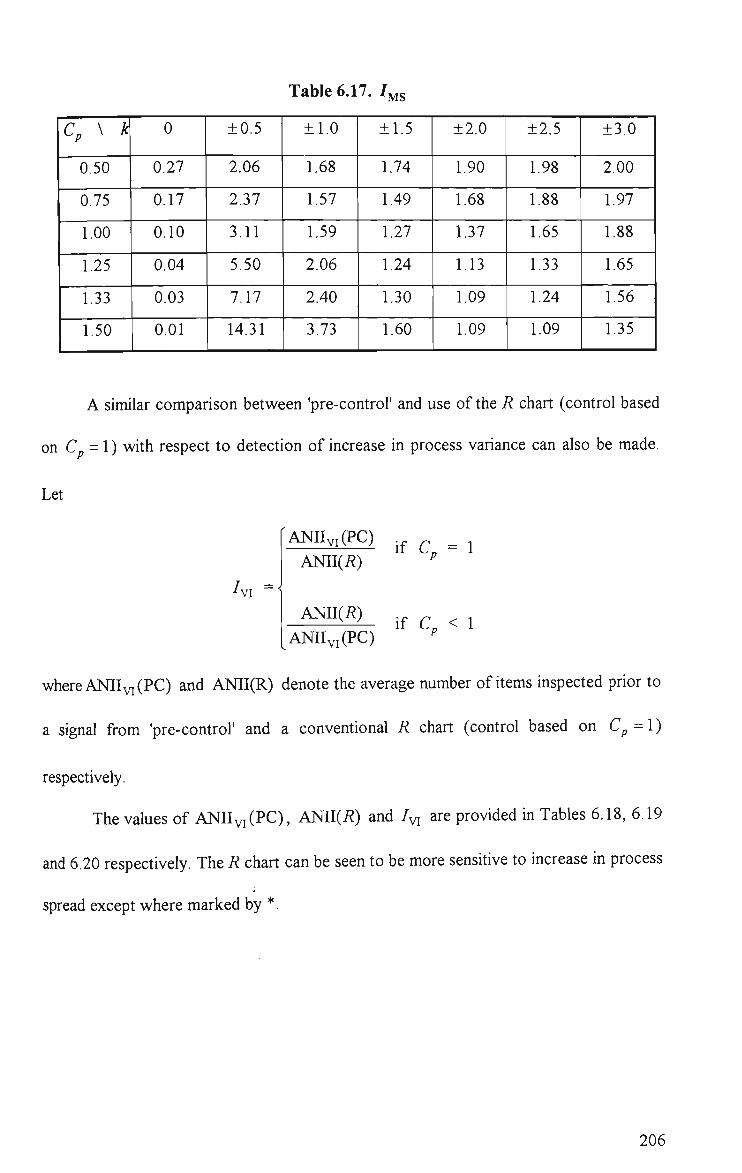
Table 6.17. / MS
Cp \ k
0.50
0.75
1.00
1.25
1.33
1.50
0
0.27
0.17
0.10
0.04
0.03
0.01
±0.5
2.06
2.37
3.11
5.50
7.17
14.31
±1.0
1.68
1.57
1.59
2.06
2.40
3.73 .,,
±1.5
1.74
1.49
1.27
1.24
1.30
1.60
±2.0
1.90
1.68
1.37
1.13
1.09
1.09
±2.5
1.98
1.88
1.65
1.33
1.24
1.09
±3.0
2.00
1.97
1.88
1.65
1.56
1.35
A similar comparison between 'pre-control' and use of the R chart (control based
on C- = 1) with respect to detection of increase in process variance can also be made.
Let
'VI
ANIIvi(PC) jf c ^ 1 ANII(i?) ^
ANII(i^) if c < 1 ANIIvi(PC) '
where AMI VI (PC) and ANII(R) denote the average number of hems inspected prior to
a signal from 'pre-control' and a conventional R chart (control based on C^ = 1)
respectively.
The values of ANIIvi(PC), ANII(i^) and /yj are provided in Tables 6.18, 6.19
and 6.20 respectively. The R chart can be seen to be more sensitive to increase in process
spread except where marked by *.
206
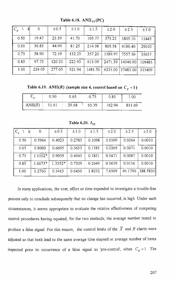
Table 6.18. ANnvi(PC)
Cp \ k
0.50
0.65
0.75
0.85
1.00
T
0
19.47
36.83
58.90
97.73
224.05
able 6.19.
Cp
ANIl(R)
Cp \ k
0.50
0.65
0.75
0.85
1.00
±0.5
23.59
44.94
72.19
120.23
277.05
±1.0
41.70
81.25
132.25
222.93
521.94
±1.5
105.77
214.38
357.20
615.09
1481.50
±2.0
375.23
805.58
1389.97
2471.39
6215.00
±2.5
1805.10
4180.40
7557.50
14040.90
37483.00
±3.0
11445
29010
55637
109485
315409
ANn(i?) (sample size 4, control based on C^ = 1)
0.50
11.61
0
0.5964
0.8060
1.1102*
1.6673*
0.2760
0.65
29.68
0.75
65.39
Table 6.20. /yi
±0.5
0.4923
0.6605
0.9059
1.3552*
0.3413
±1.0
0.2785
0.3653
0.4945
0.7309
0.6430
±1.5
0.1098
0.1385
0.1831
0.2649
1.8252
0.85
162.94
±2.0
0.0309
0.0369
0.0471
0.0659
7.6569
1.00
811.69
±2.5
0.0064
0.0071
0.0087
0.0116
46.1790
±3.0
0.0010
0.0010
0.0010
0.0010
388.5830
In many applications, the cost, effort or time expended to investigate a trouble-free
process only to conclude subsequently that no change has occurred, is high. Under such
circumstances, h seems appropriate to evaluate the relative effectiveness of competing
control procedures having equated, for the two methods, the average number tested to
produce a false signal. For this reason, the control limits of the Z and i? charts were
adjusted so that both lead to the same average time elapsed or average number of hems
inspected prior to occurrence of a false signal as 'pre-control', when Cp=l. The
207

resulting ANn(X) and ANII(i?) values are shown in Tables 6.21 and 6.22 respectively.
As illustrated in Tables 6.15 and 6.21, if the process capability is correctly assumed (i.e
C = 1) or underestimated (i.e C^ > 1), the adjusted X chart requires a much smaller
number of units, on average, to 'pick up' the given mean shift except when C_ = 1 and k
= 2, in which case the difference is marginal. For Cp - 0.5 or Cp = 0.75, h is found that
in most cases (marked whh *), 'pre-control' is marginally better than the adjusted X
chart. It can also be seen that false signals from the adjusted X chart tend to occur after
a longer period of time when the process is incapable. However, if the process is more
than capable, the adjusted X chart will tend to issue a false signal sooner than 'pre-
control' although, due to the large magnitudes, this is of little practical consequence. It
should be noted that we have delibrately omitted those cases where k = 2.5 and A: = 3.0 in
Table 6.21 because mean shifts as large as these are likely to be detected early anyway
irrespective of method. The R chart is found to be far superior to 'pre-control' in reacting
to worsening process capability (refer to Tables 6.18 and 6.22). This is especially true
when the process is not on target.
208
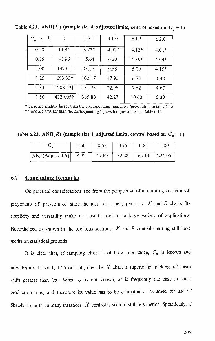
Table 6.21. ANn(Ar) (sample size 4, adjusted limits, control based on C = 1)
Cp \ k
0.50
0.75
1.00
1.25
1.33
1.50
these are slig
0
14.84
40.96
147.01
693.331
1208.12t
4329.05t
itly larger thaj
±0.5
8.72*
15.64
35.27
102.17
151.78
385.80
n the correspo
±1.0
4.91*
6.30
9.58
17.90
22.95
42.27
nding figures
±1.5
4.12*
4.39*
5.09
6.73
7.62
10.60
for 'pre-contro
±2.0
4.01*
4.04*
4.15*
4.48
4.67
5.30
r in table 6.15 *
t these are smaller than the corresponding figures for 'pre-control' in table 6.15.
Table 6.22. ANn(i?) (sample size 4, adjusted limits, control based on C = 1)
Cp
ANII( Adjusted R)
0.50
8.72
0.65
17.69
0.75
32.28
0.85
65.13
1.00
224.05
6.7 Concluding Remarks
On practical considerations and from the perspective of monitoring and control,
proponents of 'pre-control' state the method to be superior to X and R charts. Its
simplichy and versatility make h a usefiil tool for a large variety of applications.
Nevertheless, as shown in the previous sections, X and R control charting still have
merits on statistical grounds.
It is clear that, if sampling effort is of Ihtie importance, Cp is known and
provides a value of 1, 1.25 or 1.50, then the X chart is superior in 'picking up' mean
shifts greater than la . When a is not known, as is frequently the case in short
production runs, and therefore its value has to be estimated or assumed for use of
Shewhart charts, in many instances X control is seen to still be superior. Specifically, if
209

the Cp is assumed to be 1.25 but is actually between 0.5 and 1.5 then X control is
superior to 'pre-control' in 'picking up' shifts in the process mean. If Cp is assumed to
be 1, yet actually has a value somewhere between 0.5 and 1.50, then an X chart is as
good as or significantly better for detecting mean shifts than 'pre-control'. For detection
of a deterioration in the process capability we have observed the standard R chart to be
more sensitive than 'pre-control'. It would seem, therefore, that the advocacy of
Maxwell (1953) and others is sound, that in the absence of knowledge of a we can use,
for construction of standard X and R charts, an assumed Cp value of 1. Certainly this is
so in regard to providing a more sensitive instrument for process control than 'pre-
control' .
When sampling effort is important, a comparison that fairly compares the two
techniques when the sampling effort is the same, reveals that for capable processes, X
and i? charts are superior to 'pre-control'.
The material presented in this chapter has taken a perspective that focuses
narrowly on monitoring and control. Broadening the perspective and perceiving charting
techniques as merely a part in the effort of continuous improvement underscores further
the value of traditional Shewhart charts.
We have sought to create some common ground for X and R control and 'pre-
control' in order to examine their performance for monitoring and control on a statistical
basis. It is hoped that the material contained herein will provide more complete grounds
on which to base a comparison between the two techniques and thus to facihtate more
rational judgements on which of the two to use in any given situation.
210

CHAPTER 7
CONCLUSIONS AND SOME SUGGESTIONS FOR
FUTURE INVESTIGATION
7.1 Summary and Conclusions
In this thesis, some techniques for monitoring the mean vector of a muhivariate
normal process have been presented. As the proposed techniques involve sequences of
independent or approximately independent standard normal variables, the resultmg
control charts can all be plotted in the same scale and whh the same control limits
irrespective of product types, thus simplyfying charting administration. Any non-random
patterns on such standardized charts which suggest various process instabilities can also
be readily detected by the use of additional sequence rules. Those techniques presented
for the case whh no prior knowledge of process parameters are particularly attractive for
short production runs and low volume manufacturing environments since control can be
initiated essentially whh the first umts or samples of production. When used in the
context of new or long run processes, this charting approach ehminates the need for a
separate calibration study. Simulation results indicate that the techniques presented for
use with subgroup data have desirable performance whether or not the process
parameters are assumed known in advance of the production run. As for individual
values control techniques, those which do not assume known values of the process
covariance matrix Z or both the process parameters, are found to be insensitive to
sustained mean shift. However, the two alternative EWMA procedures (EWMAZl and
EWMAZIU) specifically designed for detecting this type of process change have been
demonstrated to be very effective. In addition, they are found to be far superior to some
211
competing techniques including the M charts of Chan et al.(1994) for 'pickmg up' linear
trends.
In practice, h is also of value to monitor the process dispersion as measured by
the variance-covariance matrix Z which may be subject to occasional changes. The
procedures presented for this purpose (which are based on subgroup data) involve use of
mdependent statistics resulting from the decomposition of the covariance matrix. A
simulation study indicates that the proposed techniques outperform previously proposed
procedures for many sustained shifts in Z. It has also been demonstrated that the
technique presented for the known Z case is more powerful in 'picking up' certain shifts
than that which involves the separate charting of the standardized variances of the
principal components or the individual components resulting from the decomposhion of
the covariance matrices. In addition, the proposed methods have some practical
advantages over the existing procedures. Besides providing better control over the false
alarm rate and the ease of locating the control Umhs, the proposed techniques can help
identify the nature of change in the process dispersion parameters.
In order to satisfactorily describe the capability of multivariate processes, three
muhivariate capability indices have been presented. These are based on the relative area
and position of a conservative process rectangle containing at least a specified proportion
of hems, and the specification rectangle. The development of the first involves the
projection of a process ellipse containing a specified percentage of products on to hs
component axes whereas the other two are based on the Bonferroni and Sidak
inequalities respectively. Although this work is devoted to two-sided rectangular
specifications, h can be extended to unilateral specification situations in a straightforward
manner. Some calculations that fairly compare the three reveal that the latter two are
212

superior to the former and that the Sidak-type capability index is marginally better than
that based on the Bonfertoni inequahty. A reasonable test for the Sidak-type index has
also been proposed and critical values provided for some chosen levels of significance,
sample sizes and acceptable percentages of nonconforming items. The computation of
these mdices is easier than other proposed indices and capability analysis methods.
However, as whh other muhivariate capabihty indices, h has not yet been possible to
obtain the unbiased estimators and appropriate confidence intervals for the proposed
indices except to note that for large sample sizes, h seems appropriate to replace the
parameters involved whh the usual sample estimates. A conservative type of distribution-
free capability index has also been considered. This is obtained by use of multivariate
Chebyshev-type probability inequahties. Although this is no better (more conservative)
than the Bonferroni-type capability index, the process rectangle containing at least a
specified proportion of items used for defining the index can be constructed easily for
any type of process distribution. If the underlying distribution for each quality
characteristic is known to belong to some well-known system or family of distributions
and hence appropriate quantiles may be obtained, it is advisable to consider the use of the
capability index constructed based on the Bonferroni inequality although in some cases,
this might not be practical.
A rationale for making a statistical comparison between the techniques of 'pre-
control' and tradhional X and R charts has also been provided in this thesis. Special
attention was drawn to the application of both techniques to the short run manufacturing
environment where, for the use of X and R charts, parameter estimation is a problem.
Despite hs many touted practical attributes, the results show that 'pre-control' is not as
good as the X and R charting techniques in many circumstances.
213
7.2 Suggestions for Future Work
In the following, some suggestions are made for fiiture investigation, building on
the work of this thesis.
1. A study of the robustness of the proposed mean and dispersion control procedures to
departures from the multivariate normality assumptions using run length distributions.
Convenient process models recommended for this purpose include the Elliptically
Co«/owreJ distributions (see Johnson (1987), p. 106-124) which have the multivariate
normal distributions as special cases.
2. A comparison of the statistical performance of the proposed procedures, including
EWMAZl and EWMAZIU, with the corresponding nonparametric techniques of
Hawkins (1992) for various distributional models and types of process change.
Performance criteria recommended include the run length probability, Vr{RL <k). A.
comparison could also be made between EWMAZl and the MEWMA technique of
Lowry et al.(1992).
3. A study of the properties of applying multiple univariate 'Q' charts to the principal
components and the individual quality characteristics for the cases with known and
unknown E respectively, and similar charts constructed based on independent
variables that resuh from the decomposition of the % and T statistics of (3.3) to
(3.11) in a manner similar to that of Mason et al.(1995).
4. Analysis of "?x{RL<k) for the multivariate mean control techniques based on
statistics (3.4), (3.5), (3.6), (3.8), (3.9), (3.10) and (3.11) and the proposed dispersion
control procedures for sustained shifts in p and Z respectively.
214

5. Develop dispersion control methods based on individual observations for the case
where Z is unknown and study hs RL performance relative to that of the
nonparametric procedure presented by Hawkins (1992). For the case with specified or
known Z , consideration should be made of the use of separate univariate charts
based on the variability of the principal components or some aggregate-type statistic
like those of Chapter 4 whh a comparison of the resuhing RL performance with that
of Hawkins's method.
6. Develop exact multivariate capability mdices which accurately reflect the process
status (i.e the expected proportion of usable items produced) and the expected costs
mcurred. As not all the measured characteristics are equally important in determining
the product quality in some shuations, indices which take this factor into
consideration should also be designed.
215
References
1. Adams, B. M. and WoodaU, W. H. (1989). "An Analysis of Taguchi's On-Line
Process-Control Procedure Under a Random-Walk Model". Technometrics 13, pp.
401-413.
2. Al-Salti, M. and AspinwaU, E. M. (1991). "Movhig Average Moving Range and
CUSUM Modelling in SmaU Batch Manufacturing". Proceedings of 3rd Conference
of Asia Pacific Quality Control Organisation.
3. Al-Salti, M., and Statham, A. (1994). "A Review of the Lherature on the Use of SPC
in Batch Production". Quality and Reliability Engineering International 10, pp. 49-
61.
4. Al-Salti, M., AspinwaU, E. M. and Statham, A. (1992). "Implementing SPC in a Low-
volume Manufacturing Environment". Quality Forum 18, pp. 125-132.
5. Alt, F. B. and Bedewi, G. E. (1986). 'SPC of Dispersion for Multivariate Data'. ASQC
Quality Congress Transaction - Anaheim. American Society for Quality Control, pp.
248-254.
6. Alt, F. B. and Smith, N. D. (1990). "Multivariate Quality Control' in Handbook of
Statistical Methods for Engineers and Scientists, Ed. H.M. Wadsworth, McGraw-
Hill, New York, NY.
7. Alt, F. B.; Goode, J. J. and Wadsworth, H. M. (1976). 'SmaU Sample Probability
Limits For the Mean of a Multivariate Normal Process'. ASQC Technical Conference
Transactions - Toronto. American Society for Quality Control, pp. 170-176.
8. Anderson, T. W. (1984). An Introduction to Multivariate Statistical Analysis, 2nd
ed., John WUey & Sons, New York, NY.
9. Armitage, S. J. and Wilharm, M. T. (1988). "Techniques For Expanding The Sphere
of Statistical Process Control". Tappi Journal, July, pp.71-77.
lO.Barnett, N. S. (1990). 'Process Control and Product Quality - The C^ and C^A:
Revisited'. International journal of Quality and Reliability Management, Vol.7,
No.4, pp.34-43.
11.Bather, J. A. (1963). "Control Charts and Minimization of Costs". Journal of Royal
Statistical Society, Series B 25, pp. 49-80.
216
12.Bayer, H. S. (1957). "Quality Control AppUed to a Job Shop". ASQC National
Convention Transactions, pp. 131-137.
O.Bhote, K. E. (1980). World Class Quality, AMA Management Briefing.
M.Bothe, D. R. (1989). "A Powerfiil New Control Chart for Job Shops". ASQC 43rd
Annual Quality Congress Transactions, pp. 265-270.
15.Bothe, D. R. (1990). "A Control Chart for Short Production Runs". Quality Australia
7, pp. 19-20.
16.Bothe, D. R. (1990). "SPC For Short Production Runs". Quality Australia 7, pp. 53-
56.
17.B0X, G. E. P. and Jenkins, G. M. (1963). "Further Contributions to Adaptive Quality
Control : Simuhaneous Estimation of Dynamics : Non-Zero Costs". Bulletin of the
International Statistical Institute 34, pp. 943-974.
IS.Box, G E. P., Jenkins, G. M. and MacGregor, J. F. (1974). "Some Recent Advances
in Forecasting and Control, Part II". Applied Statistics 23, pp. 158-179.
19.Boyles, R. A. (1991). 'The Taguchi Capability Index'. Journal of Quality Technology,
Vol.23, No. 1, pp. 17-26.
20.Boyles, R. A. (1994). 'Covariance Models for Repeated Measurements with Lattice
Structure'. Submitted for publication.
21.Boyles, R. A. (1996). 'Exploratory Capability Analysis'. Journal of Quality
Technology, Vol.28, No.l, pp.91-98.
22.Brown, N. R. (1966). "Zero Defects the Easy Way with Target Area Control".
Modern Machine Shop, July, pp. 96-100.
23.Burr, I. W. (1954). "Short Runs". Industrial Quality Control, September, pp. 17-22.
24.Burr, I. W. (1976). Statistical Quality Control Methods. Marcel Dekker Inc.,
Milwaukee, Wisconsin.
25.Burr, J. T. (1989). "SPC in The Short Run". ASQC 43rd Annual Quality Congress
Transactions, pp. 776-780.
26.Calvin, J. A. (1994). 'One-sided Test of Covariance Matrix with A Known Null
Value'. Communications in Statistics - Theory and Methods 23, pp.3121-3140.
27.Castillo, E. D. (1995). Discussion o f 'Q ' Charts. Journal of Quality Technology 27,
pp.316-321.
217

28.Castillo, E. D. and Montgomery, D. C. (1994). "Short-Run Statistical Process
Control : Q-Chart Enhancements and Alternative Methods". Quality and Reliability
Engineering International 10, pp. 87-97.
29.Castillo, E. D. and Montgomery, D. C. (1995). 'A Kalman Filtering Process Control
Scheme with An Application in Semiconductor Short Run Manufacturing'. Quality
and Reliability Engineering International 11, pp. 101-105.
30.Chan, L. K. and Li, Guo-Ying. (1994). 'A Multivariate Control Chart for Detecting
Linear Trends'. Communications in Statistics - Simulation and Computation 23,
pp.997-1012.
31.Chan, L. K.; Cheng, S. W. and Spiring, F. A. (1988). 'A Graphical Technique for
Process Capability'. ASQC Quality Congress Transactions - DaUas, pp.268-275.
32.Chan, L. K.; Cheng, S. W. and Spiring, F. A. (1990). 'A Multivariate Measure of
Process Capability'. International Journal of Modeling and Simulation 11, pp. 1-6.
33.Chen, J. and Gupta, A. K. (1994). 'Likelihood Procedure for Testing Change Points
Hypothesis for Multivariate Gaussian Model'. Technical Report No.94-01, Dept. of
Mathematics & Statistics, Bowling Green State University.
34.Chen, J. and Gupta, A. K. (1994). 'Estimation and Testing of Change Points for
Covariance in Multivariate Gaussian Model'. Proceedings of the International
Conference on Statistical Methods and Statistical Computing for Quality and
Productivity Improvement (ICSQP '95), pp.405-432.
35.Clements, J. A. (1989). Process Capabihty Calculations for Non-Normal
Distributions'. Quality Progress, September, pp.95-100.
36.Cook, H. M. Jr. (1989). "Some Statistical Control Techniques for Job Shops". 43rd
Annual Quality Congress Transactions, pp. 638-642.
37.Crichton, J. R. (1988). "Guidelines and Techniques for Applying Control Charts in a
Batch Operation". Tappi Journal, December, pp. 91-95.
38.Crosier, R. B. (1988). 'Multivariate Generalization of Cumulative Sum Quality-
Control Schemes'. Technometrics 30, pp. 291-303.
39.Crowder, S. V. (1989). 'An Application of Adaptive Kalman Fihering to Statistical
Process Control', in Statistical Process Control in Automated Manufacturing, Eds. J.
B. Keats &. N.F. Hubele, Marcel Dekker, New York, NY.
218

40.Crowder, S. V. (1992). 'An SPC Model For Short Production Runs : Minimizing
Expected Cost'. Technometrics 34, pp. 64-73.
41.Cryer, J. D. and Ryan, T. P. (1990). 'The Estimation of Sigma For an X Chart :
M ^ d j or S/C4 1\ Journal of Quality Technology 22,1^^. 187-192.
42.Das-Gupta, S. (1969). 'Properties of Power Functions of Some Tests Concerning
Dispersion Matrices of Multivariate Normal Distributions'. Annals of Mathematical
Statistics 40, pp.697-701.
43.Davis, A. W. and Field, J. B. F. (1971). 'Tables of Some Multivariate Test Criteria'.
Technical Paper ^0. 32, C.S.I.R.O, Australia.
44.Doganaksoy, N.; Faltin, F. W. and Tucker, W. T. (1991). 'Identification of Out Of
Control Quality Characteristics in a Muhivariate Manufacturing Environment'.
Communications in Statistics - Theory and Methods 20, pp. 2775-2790.
45.Doganaksoy, N.; Schmee, J. & Vandeven, M. (1996). 'Process Monitoring with
Multiple Product Grades'. Journal of Quality Technology 28, pp.346-355.
46.Ermer, D. S. and Born, D. D. (1989). "Statistical Process Control for Short
Production Runs : AX-MR Control Charts". Quality Improvement Techniques For
Manufacturing, Products And Services, Eds. A.H. Abdelmonem, AT & T Bell
Laboratories, pp.43-87.
47.Farnum, N. R. (1992). "Control Charts for Short Runs: Nonconstant Process and
Measurement Error". Journal of Quality Technology 24, pp. 138-144.
48.Farnum, N. R. (1995). Discussion of 'Q ' Charts. Journal of Quality Technology 27,
pp.322-323.
49.Fisher, R. A. (1950). Statistical Methods for Research Workers, London : Oliver and
Boyd.
SO.Folks, J. L. (1984). 'Combination of Independent Tests', in Handbook of Statistics,
Vol.4, Eds. P. R. Krishnaiah and P. K. Sen, Elsevier Science Pubhsher.
51.Foster, G. K. (1988). 'Implementing SPC in Low Volume Manufacturing'. ASQC
Annual Quality Congress Transactions, pp. 261-267.
52.Franklin, L. A. and Wasserman, G. S. (1992). 'Bootstrap Lower Confidence Limits
for CapabUity Indices'. Journal of Quality Technology 24, pp. 196-210.
53.Giri, N. C. (1977). Multivariate Statistical Inference, Academic Press, New York,
NY.
219

54.Gnanadesikan, R. (1977). Methods for Statistical Data Analysis of Multivariate
Observations, John Wiley & Sons, New York, NY.
55.Ghosh, B. K.; Reynolds, M. R. Jr and Hui, Y. V. (1981). 'Shewhart J-Charts with
Estimated Process Variance'. Communications in Statistics - Theory and Methods 10,
pp. 1797-1822.
56.Grant, E. L. and Leavenworth, R. S, (1980). Statistical Quality Control, 5th ed.,
McGraw-Hill, New York, NY.
57.GraybiU, F. A. (1983). Matrices with Applications in Statistics, 2nd ed., Wadsworth
Inc., Belmont, CA.
58.Hawldns, D. L. (1992). 'Detecting Shifts in Functions of Multivariate Location and
Covariance Parameters'. Journal of Statistical Planning and Inference 33, pp.233-
244.
59.Hawkins, D. M. (1981). 'A CUSUM for A Scale Parameter'. Journal of Quality
Technology 13, pp.228-231.
60.Hawkins, D. M. (1987). 'Self-Starting Cusum Charts for Location and Scale'. The
Statistician 36, pp.299-315.
61.Hawkins, D. M. (1991). 'Multivariate Quality Control Based on Regression-Adjusted
Variables'. Technometrics 33, pp. 61-75.
62.Hawkins, D. M. (1993a). 'Regression Adjustment for Variables in Multivariate
Quality Control'. Journal of Quality Technology 25, pp. 170-182.
63.Hawkins, D. M. (1993b). 'Robustification of Cumulative Sum Charts by
Winsorization'. Journal of Quality Technology 25, pp. 248-261.
64.Hawkins, D. M. (1995). 'Discussion o f 'Q ' Charts. Journal of Quality Technology
27, pp.324-327.
65.Hayter, A. J. and Tsui, K. (1994). 'Identification and Quantification in Multivariate
Quality Control Problems'. Journal of Quality Technology 26, pp. 197-208.
66.Healy, J. D. (1987). 'A Note on Muhivariate CUSUM Procedures'. Technometrics
29, pp.409-412.
67.HiUier, F. S. (1964). 'X Chart Control Limits Based on A Small Number of
Subgroups'. Industrial Quality Control, February, pp.24-29.
68.HiUier, F. S. (1967). 'SmaU Sample Probability Limits for the Range Chart'.
American Statistical Association Journal, December, pp. 1488-1493.
220
69.Hillier, F.S. (1969). 'X andR Chart Control Limits Based On a Small Number of
Subgroups'. Journal of Quality Technology 1, pp. 17-26.
70.Ho, C. and Case, K. E. (1994). 'Economic Design of Control Charts : A Literature
Review for 1981-1991'. Journal of Quality Technology 26, pp.39-53.
71.Hogg, R. V. and Craig, A. T. (1971). Introduction to Mathematical Statistics, 3rd
ed., The Macmillan Co., New York, NY.
72.Holmes, D. S. and Mergen, A. E. (1993). 'Improving the Performance of the T^
Control Chart'. Quality Engineering, Vol.5, No.4, pp.619-625.
73.Hotelling, H. (1947). 'Multivariate Quality Control' in Techniques of Statistical
. Analysis, Eds. Eisenhart, Hastay and Wallis. McGraw-Hill, New York, NY.
74.Hubele, N. F.; Shahriari, H. and Cheng, C-S. (1991). 'A Bivariate Process Capability
Vector', in Statistical Process Control in Manufacturing, Eds. JB. Keats and D.C.
Montgomerry, Marcel Dekker, New York, NY & ASQC Press, Milwaukee,
Wisconsin.
75.Jackson, J. E. (1991). 'Multivariate Quality Control : 40 Years Later' in Statistical
Process Control in Manufacturing, Eds. J.B. Keats and D.C. Montgomery, Marcel
Dekker NY and ASQC Quality Press Wisconsin.
76. Johnson, M. E. (1987). Multivariate Statistical Simulation. John WUey & Sons, New
York, NY.
77.Johnson, N. L. and Kotz, S. (1970). Distributions in Statistics : Continuous
Univariate Distributions 1, Vol.2, John Wiley & Sons, New York, NY.
78.Johnson, N. L. and Kotz, S. (1972). Distributions in Statistics : Continuous
Multivariate Distributions, Vol.4, John Wiley & Sons, New York, NY.
79. Johnson, R. A. and Wichern, D. W. (1988). Applied Multivariate Statistical Analysis,
2nd ed., Prentice-Hall, Englewood Cliffs, NJ.
SO.Kane, V. E. (1986). 'Process Capability Indices'. Journal of Quality Technology,
Vol.18, No.l, pp.41-52. Corrigenda p.265.
Sl.Kiefer, J. and Schwartz, R. (1965). 'Admissible Bayes Character of T^ - and R^ -
and Other Fully Invariant Tests for Classical Normal Problems'. Annals of
Mathematical Statistics 36, pp.747-760.
82.King, E. P. (1954). "Probability Limhs for The Average Charts When Process
Standards Are Unspecified". Industrial Quality Control, May, pp. 62-64.
221
83.Koons, G. F. and Luner, J. J. (1991). "SPC m Low Volume Manufacturing : A Case
Study". Journal Of Quality Technology 23, pp. 287-295.
84.Koziol, J. A. and Periman, M. D. (1978). 'Combining Independent Chi-Squared
Tests'. Journal of the American Statistical Association 73, pp.753-763.
85.Kushler, R. H. and Huriey, P. (1992). 'Confidence Bounds for Capability Indices'.
Journal of Quality Technology, Vol.24, No.4, pp. 188-195.
86.Lancaster, H. O. (1961). 'The Combmation of Probabilities : An Apphcation of
Orthonormal Functions'. Australian Journal of Statistics, Vol.3, pp.20-33.
87.Lehmann, E. L. (1959). Testing Statistical Hypotheses, John WUey & Sons, New
York, NY.
88.Lill, M. H., Yen Chu and Ken Chung. (1991). "Statistical Setup Adjustment for Low
Volume Manufacturing", in Statistical Process Control in Manufacturing, Eds. J.B.
Keats & D.C. Montgomery, Marcel Dekker, New York, NY & ASQC Quality Press,
Milwaukee, Wisconsin.
89.Lindgren, B. W. (1976). Statistical Theory, 3rd ed., MacmiUan PubUshing Co., New
York, NY.
90.Logothetis, N. (1990). "The Theory of Pre-Control : A Serious Method or A
Colourful Naivity ?". Total Quality Management I, pp.207-220.
91.Lowry, C. N. (1989). 'A Multivariate Exponentially Weighted Moving Average
Control Chart'. Ph.d thesis. University of Southwestern Louisiana, U.S.A.
92.Lowry, C. N. and Montgomery, D. C. (1995). 'A Review of Multivariate Control
Charts'. HE Transactions 27, pp.800-810.
93.Lowry, C. N.; Woodall W. H.; Champ, C. W. and Rigdon, S. E. (1992). 'A
Multivariate Exponentially Weighted Moving Average Control Chart'. Technometrics
34, pp. 46-53.
94.MacGregor, J. F. and Harris, T. J. (1993). 'The Exponentially Weighted Moving
Variance'. Journal of Quality Technology 25, pp. 106-118.
95.Marcucci, M. O. and Beazley, C. C. (1988). 'Capability Indices : Process Performance
Measures'. ASQC Quality Congress Transactions, American Society for Quality
Control, pp.516-523.
96.Marden, J. I. (1982). 'Combining Independent Noncentral Chi Squared Or F Tests'.
The Annals of Statistics 10, pp.266-277.
222

97.Mason, R. L.; Tracy, N. D. and Young, J. C. (1995). 'Decomposition of T^ for
Multivariate Control Chart Interpretation'. Journal of Quality Technology 27, pp.99-
108.
98.MaxweU, H.E. (1953). A Simplified Control Chart For The Job Shop. Industrial
Quality Control, November, pp.34-37.
99.Montgomery, D. C. (1980). "The Economic Design of Control Charts : A Review
and Lherature Survey". Journal of Quality Technology 12, pp.75-87.
lOO.Montgomery, D. C. and Wadsworth, H. M. (1972). 'Some Techniques For
Muhivariate Quality Control Applications'. Annual Technical Conference
Transactions, American Society for Quality Control, pp.427-435.
10I.Morrison, D. F. (1976). Multivariate Statistical Methods, 2nd ed., McGraw-HiU,
New York, NY.
102.Murphy, B. J. (1987). 'Selecting Out of Control Variables with the T^ Multivariate
Quality Control Procedure'. The Statistician 36, pp.571-583.
103 .Murray, I. and Oakland, J.S. (1988). 'Detecting Lack Of Control In A New, Untried
Process'. Quality And Reliability Engineering International, Vol.4, pp.331-338.
104.Nagao, H. (1967). 'Monotonicity of the Modified Likelihood Ratio Test for a
Covariance Matrix. Journal of Science Hiroshima University A1 31, pp. 147-150.
105.Nelson, L. S. (1982). "Control Charts for Individual Measurements". Journal of
Quality Technology 14, pp. 172-173.
106.Nelson, L. S. (1984). "The Shewhart Control Chart Tests for Special Causes".
Journal of Quality Technology 16, pp. 237-239.
107.Nickerson, D. M. (1994). 'Construction of a Conservative Region From Projections
of an Exact Confidence Region in Multiple Linear Regression'. The American
Statistician 48, pp. 120-124.
108.Nomikos, P. and MacGregor, J. F. (1995). 'Muhivariate SPC Charts for Monitoring
Batch Processes'. Journal of Quality Technology 37, pp.41-59.
109.Nugent, B. A. (1990). "SPC in Short Run Processes". Proceedings of The IEEE
1990 National Aerospace and Electronics Conference - Dayton, Ohio, USA.
pp. 1304-1307.
223
llO.Pearn, W. L,; Kotz, S, and Johnson, N. L. (1992). 'Distributional and Inferential
Properties of Process Capabihty Indices'. Journal of Quality Technology 24, pp.216-
231.
111.PignatieUo, J. J. Jr and Runger, G C. (1990). 'Comparisons of Muhivariate
CUSUM Charts'. Journal of Quality Technology 22, pp. 173-186.
112.Press, S. J. (1982). Applied Multivariate Analysis : Using Bayesian and Frequentist
Methods of Inference, 2nd ed., Robert E. Krieger PubUshing Co., Malabar, FL.
113.Putnam, A.O. (1962). Pre-Control. Quality Control Handbook, 2nd edition, Eds.
Juran, J.M., Seder, L.A. & Gryna, F.M. Jr., McGraw-HiU Inc.
IH.Quesenberry, C. P. (1991a). 'SPC Q Charts for Start-Up Processes and Short or
Long Runs'. Journal of Quality Technology 23, pp.213-224.
115.Quesenberry, C. P. (1991b). 'SPC Q Charts for a Binomial Parameter : Short or
Long Runs'. Journal of Quality Technology 23, pp.239-246.
116.Quesenberry, C. P. (1991c). 'SPC Q Charts for a Poisson Parameter : Short or Long
Runs'. Journal of Quality Technology 23, pp. 296-3 03.
IH.Quesenberry, C. P. (1993). 'The Effect of Sample Size on Estimated Limits for X
and X Control Charts'. Journal of Quality Technology 25, pp. 237-247.
118.Quesenberry, C. P. (1995a). 'On Properties of Q Charts for Variables'. Journal of
Quality Technology 27, pp. 184-203.
119.Quesenberry, C. P. (1995b). 'On Properties of Binomial Q Charts for Attributes'.
Journal of Quality Technology 27, pp.204-213.
120.Quesenberry, C. P. (1995c). 'On Properties of Poisson Q Charts for Attributes'.
Journal of Quality Technology 27, pp.293-303.
121.Quesenberry, C. P. (1995d). Response to Discussions of 'Q' Charts. Journal of
Quality Technology 27, pp.333-343.
122.Robinson, G. (1991). "SPC for Short Production Runs: An Example". Quality
Australia 8, pp. 55-57.
123.Robinson, G, Touw, J. V. D. and Veevers, A. (1993). "Control Processes, Not
Products". The Quality Magazine, June, pp.88.
124.Rodriguez, R. N. (1992). 'Recent Developments in Process Capability Analysis'.
Journal of Quality Technology 24, pp. 176-187.
224
125.Roes, K. C. B., Does, R. J. M. M. and Schurink, Y. (1993). "Shewhart-Type
Control Charts for Individual Observations". Journal of Quality Technology 25, pp.
188-198.
126.Satterthwahe, F.E. (1973). 'Pre-Control For Supervisors'. Quality Progress,
February, pp.26-28.
127.Scholz, F. W. and Tosch, T. J. (1994). 'SmaU Sample Uni- and Multivariate Control
Charts for Means'. American Statistical Association 1994 Proceedings of the Section
on Quality and Productivity.
128. Sealy, E.H. (1954). A First Guide To Quality Control For Engineers, Her Majesty's
Stationery Office, UK., pp.22-23.
129.Shainin, D. (1954). Chart Control Without Charts — Simple, Effective J. & L.
Quality Pre-Control. ASQC Quality Convention Paper, American Society For Quality
Control, pp.405-417.
130.Shainin, D. (1965). Techniques For Maintaining A Zero Defects Program. AMA
Management Bulletin, Vol.71, pp. 16-21.
131.Shainin, D. (1984). Better Than Good OidXScR Charts Asked By Vendees. ASQC
38th Quality Congress Transactions - Chicago, American Society For Quality
Control, pp.302-307.
132. Shainin, D. (1990). Pre-Control. Quality Control Handbook, 4th edition, Ed. Juran,
J.M., McGraw-HiU Inc.
13 3. Shewhart, W. A. (1931). Economic Control of Quality of Manufactured Product.
D. van Nostrand Co. Inc., New York, NY.
134. Sidak, Z. (1967). 'Rectangular Confidence Regions for the Means of Multivariate
Normal Distributions'. Journal of the American Statistical Association 62, pp.626-
633.
135.Sinibaldi, F.J. (1985). Pre-Control, Does It Really Work With Non-Normality.
ASQC Quality Congress Transactions - Baltimore, American Society For Quality
Control, pp.428-433.
136.Sparks, R. S. (1992). 'Quality Control with Multivariate Data'. Australian journal
of Statistics 34, pp.375-390.
137.Srivastava, M. S. and Khatri, C. G (1979). An Introduction to Multivariate
Statistics, Elsevier North Holland, New York, NY.
225

138.Stein, C. (1956). 'The AdmissibUity of HotelUng's 7^-test'. Annals of
Mathematical Statistics 27, pp.616-623.
139.SuUivan, J. H. and Woodall, W. H. (1995). 'A Comparison of Multivariate Quality
Control Charts for Individual Observations', accepted for publication in Journal of
Quality Technology.
HO.Taguchi, G. (1981). On-Line Quality Control Control During Production. Tokyo,
Japanese Standards Association.
141.Taam, W.; Subbaiah, P. and Liddy, J. W. (1993). 'A Note on Multivariate Capability
Indices'. Journal of Applied Statistics 20, pp.339-351.
142.Tang, P. F. (1995). 'Mean Control for Multivariate Processes with Specific
Reference to Short Runs'. International Conference on Statistical Methods and
Statistical Computing for Quality and Productivity Improvement - Seoul. The
International Statistical Institute (ISI), pp.579-585.
143.Thomas, D. E. (1990). "The Balance Chart : A New SPC Concept". Quality And
Reliability Engineering International 6, pp. 357-371.
144.Thompson, L. A. Jr. (1989). "SPC and The Job Shop". ASQC 43rd Annual Quality
Congress Transactions, pp. 896-901.
145.Tippett, L. H. C. (1931). The Method of Statistics, London : Williams andNorgate.
146.Tracy, N. D.; Young, J. C. and Mason, R. L. (1992). 'Multivariate Control Charts
for Individual Observations'. Journal of Quality Technology 24, pp.88-95.
147.Traver, R.W. (1985). 'A Good Alternative To X-R Charts'. Quality Progress,
September, pp. 11-14.
148.Trigg, D. W. and Leach, A. G. (1967). 'Exponential Smoothing with An Adaptive
Response Rate'. Operational Research Quarterly 18, pp. 53-59.
149.WaUace, D. L. (1959). 'Bounds on Normal Approximations to student's and the
Chi-square Distributions'. Annals of Mathematical Statistics 30, pp. 1121-1130.
150.Wasserman, G S. (1994). 'Short Run SPC Using Dynamic Control Chart'.
Computers and Industrial Engineering 27, pp.353-356.
151.Wasserman, G S. and Sudjianto, A. (1993). 'Short Run SPC Based Upon the
Second Order Dynamic Linear Model for Trend Detection'. Communications in
Statistics - Simulation and Computation 22, pp. 1011-1036.
226
152.Wierda, S. J. (1994). 'Multivariate Statistical Process Control - Recent Resuhs and
Directions for Future Research'. StatisticaNeerlandica 48, pp. 147-168.
153.Wolfram, S. (1991). Mathematica : A System for Doing Mathematics by Computer,
2nd ed., Addison-Wesley, Redwood City, CaUfomia.
154.WoodaU, W. H. and Ncube, M. M. (1985). 'Multivariate CUSUM Quality-Control
Procedures'. Technometrics 21, pp.285-292.
155.Woodall, W. H.; Crowder, S. V. and Wade, M. R. (1995). Discussion of'Q' Charts.
Journal of Quality Technology 27, pp.328-332.
156.Woodward, P. W. and Naylor, J. C. (1993). "An Apphcation of Bayesian Methods
in SPC". The Statistician 42, pp.461-469.
157.Yang, C. H. and HiUier, F. S. (1970). "Mean and Variance Control Chart Limits
Based On a SmaU Number of Subgroups". Journal of quality Technology 2, pp.9-16.
227
Appendices
A.1 Dependence of Statistical Performance on the Noncentrality Parameter, X
for a Step Shift in Process Mean Vector
Assume that the process variance-covariance matrix, Z is constant but that the
process mean vector may change from p to p„^ at an arbhrary point in time. It is
shown below that for the same change point i.e the observation or subgroup number
after which the shift occurs, the joint distribution of the T^ 's (or equivalently, Z 's) and
hence the statistical performance of the control techniques presented in section 3.3 of
Chapter 3 depends on p , p„g^ and Z only through the value of the noncentrality
parameter.
To estabUsh the proof for the above, use is made of the foUowing lemmas and theorems
which are adapted from Crosier (1988) and Lowry (1989).
Lemma 1
If X:=MX,, x r = M ( X , - p ) , X;.=MX^. and X " = M ( x ^ . - p ) , k^l,2,...,
j = l,2,...,n where Mis a pxp matrix of fliU rank, then the relevent 7; statistics have
the same values whether they, are computed from X^, (X; - p), X , and (X , - p) or
the corresponding transformed vectors X*, X", X^ andXj*, i.e, the j ; statistics are
invariant whh respect to these transformations. In other words, a fiiU rank linear
transformation of the observation vectors or their deviations from target (known mean
vector) has no effect on the 7j statistics.
228

Proof: Immediate.
Lemma 2
If X:=MX„ x r = M ( X , - p ) , X;.=MX^. and X * = M(X;,. - p), ^ = 1,2,...,
j = 1,2,...,n where Misa px p matrix of fliU rank, then
ii*=E{xl) = E{xl) = ^ i l = M p
^iL=Mp,
k<r
, k>r
p**=4xr)=4x-)= PZ = 0 , k<r
^l^l=M(p„^^-p) ,k>r
where r is the observation or subgroup number after which the process mean vector
changes from p to p„^. Thus,
(n:: - i^zf r'~\viZ - P::)=(P„. - r Z-XP„^ - P)
Proof: Immediate.
This resuh implies that the noncentrality parameter has the same value whether
computed from the original dependent variables or from some Unearly independent
combinations of them (or their deviations from targets or known means).
229
Lemma 3
If (^iw-^il)^S"'H^^w-^^l) = (^^2^-^A2f S~H^^2^.-^i2)> there exists a
nonshigular matrix M such that
( ^ i w - ^ i l ) = M ( p 2 _ - P 2 )
M Z M ' ^ = Z
Proof:
First, transform each variable of the form (X^^,. -X , ^^) to Y, principal components
scaled to have unit variances where X ^ ^ and X , ^ respectively denote observation
vectors before and after the change in the process mean vector. Let E(Y) = V, by
lemma 2,
Vi Vi = V^V^ where % = D"'p(pi_ - p^)
V 2 = D " ' P ( P 2 _ - P 2 )
and P is an orthogonal matrix that diagonaUzes Zrv , _v„, i giving ' - ' "- (•'^ After ^Befortl ^ ^
PZ.v X ,P^ = D
C After ~^ Befon )
Hence, there exists an orthogonal matrix Q such that
V,=QV,
Upon substituting Vi = D"^P(pi„^ - Pi) and Vj = D~P(p2_ - P2) into the equation
above, M is obtainable as follows :
230
= P^D^QD-P(p ,_-P , )
Now, h is shown that MZM^ = Z . We have
MZfx X ^M"" '^'^After ^Before'
=>
=>
M(2Z)M^
M Z M ^
= P^D^QD"
= P^D^QD
= P^DP
^^After~^Befi
= 2Z
=z.
"PZ,
^DD
,«)
•^After~^Before
^Q^D^P
)P^D ^Q^D^P
(Q.ED.)
This lemma is also applicable to cases with known p, namely, if
(^il«^-^i) 5:"^(pi_-p) = (p2„«.-^i) 2~'(p2„.«-n), there exists a nonsingular
matrix M such that
MZM'^ = Z.
The proof for this is similar to the above except that Pi and pj should both be replaced
by p.
231
Theorem 1
For the cases with unknown p, if
T v l i (^ iw-^ i I ) 2:"X^iw-^ll)=(^i2. .-^A2) 2"'(n2™»-iLi2),
then/7;'54x,orX^.) = r ^ Pi ,k<r
^iw .^>0 - / r,'54x,orX^.) =
P2 ,k<r
.^i2«. , ^ > ' ' .
where / r,' 4x,orX .) = 'Pi ,A:<r denotes the joint pdf of 7 ' 5 given
£(x,) = 4x,,) =
and / Tk'^ / X rp2 ,^^^1
EyXj^ or X^ \ = < denotes the joint pdf of 7 ' 5 given
£(x,) = 4x,,) = 'P2 ,k<r
where r is the change point. This theorem implies equivalent performance of the control
techniques under the two alternative probability densities.
Proof:
Note that the T^'s of (3.3), (3.6), (3.8) and (3.11) are expressible either in terms of
random vectors of the form ( x ^ - X ^ j for p^q or (x^ , -X^ j for p^q,
i,j = 1,2,...,n and p = q, i'^j, i,j = 1,2,...,n. Let pdf 1 refer to the multivariate
normal density specified by
E(X,)=E{X^)= 'Pi ,k<r
> i „ ,k>r
md pdf 2 refer to the multivariate normal density specified by
232

E(X,)=E{X^) = P2 ,k<r
M2r.. ^>r
If pdf 2 is expressed in the transformed variates Z^=MX^ (orZ^^MXK) where
1 1
M = P^D»QD 'P is as given in lemma 3, then Far(Zi) = Far(Zj,) = M I M ' ' = 1 and
£ ( Z , - Z , ) = 4 z , , - Z ^ )
0 if p,q < r 01 p,q>r
^Aw-^il ifp>r,q<r
l^Ai-iiw ifp<r,q>r
It can also easily be shown that the covariance of the transformed variates (Zp-Z^)
and (Z_j-Zf) under pdf 2 is the same as the covariance of (x^ -X^)
[(X,, - X^.)]and (X, - X,) [(X,, - X^)] underpJ/1, i.e
Cov[(z^ -Z , ) , (Z , -Z, ) ] = C^(X^ -X,),(X, -X,)]
xmdei pdf 2 under pdf I
'Cov[(Zp, -Z^),(Z,„ -Z^) ] = Cov[(x^, -X^),(X,„ -X^)[^
uadcT pdf 2 nndQrpdfl
for aWp, q, s and t (p, q, s, t, i,j, u and v). Hence, pdf 2 expressed in the transformed
variates Z^ ( Z^) is the same as pdf I expressed in X^ P^ig) variates, i.e
/ TJ^ E{x,orX^.) = Vl ,k<r
Mu ,k>r = f Tk'^ 4z,orz^.)=|; Mp2
MP2«. ,
,k<r
k>r (A. 1.1)
By lemma 1, the values of the 7 '5 are invariant whh respect to the transformation from
X, (X^.)toZ^(Z^^.)sothat ,
/ Tk's (x^orX^.) = j P2 ,k<r
^2r^ ,k>rj -f Tk's 'i^^-^HZ:jT>rj (A. 1.2)
233

Combining (A. 1.1) and (A. 1.2) gives
/ Tk's 4 x , o r X , ) = ' f ; l = / f r , ' . 4 x , o r X , > ^ 'f^"
Therefore, the joint distribution of 7 '5 given p^ and Pj„^ (and Z) is the same as the
joint distribution of 7 '5 given P2 and P2„«, (and Z) if
T ^ - l i {y-lne.-S^l) 2 : \\i'lr..-\i-l)^{\i.2ne.-\^2) ^ ^ 1 ^ 2 ^ ^ " 1 ^ 2 )
(Q.ED.)
Theorem 1 can be adapted to cases with known p, namely, if
T v - l i i^lne^-p) 2 \[il„e.-li) = (P2ne.-\^) ^ ^ ( p 2 „ ^ " p ) , thCU
/ Tk'^ 4x,orX,)J^ fj^ = f Tk's 4x,orX,)J^ '7/.
The proof for this is similar to the above except that X^ (X^) and P,„^ - p , , ' = 1,2
should be replaced by X^ - p (X^ - p) and p,„^ - p respectively.
234

Theorem 2
For the cases with unknown p , let X^,^'s (Xj^'j) be independent observation vectors
frompdfl and Xj^t'^ 0^2k;'^) be independent observation vectors ^ompdf2. Letpdfl
he multivariate normal with mean vector pj and Pi„_ before and after the change and
variance-covariance matrix Zi- Let pdf 2 be multivariate normal with mean vector P2
and P2„„ before and after the change and variance-covariance matrix Z2 • Denote the
change point by r. If (pi^^ - p^)"^ Z r ' ( l i u . - V-x) = (! 2«.w - ^A2) ^'^{s^ine^ ' 1^2). then
fi{Tk's) = f2{Tks) where fi{T^'s) and f2{TkS) represent the joint distribution of T '5
given/JfiJ l and p t ^ 2 respectively.
Proof
Let X\, = D~'PiXi, (x:,^. = D-'PjX J and X^, = D ; ' P 2 X 2 , (X^,^ = D2'P2X2;^.
where Pj and Pj are matrices that diagonalize Z(Xip-Xi,) (o^ 2](Xip,-x,^)) ^nd
^(x,,-x,,) (or 2:(x,,,-x,,.))> /^'^^ respectively, i.e
'1 2](Xip-XiJ I*i2]rx,„-x,„)Pi - ^ 1
P2S(X2„-X2jI*2 -1^2
Then,
E[x\p-X\^)=\i\p-K 1 . = ^
D:'Pi(Pw-iii) , p > ^ ^ ^ ^
D ; ^ P I ( P I - P I J .P<r,q>r
0 elsewhere
235
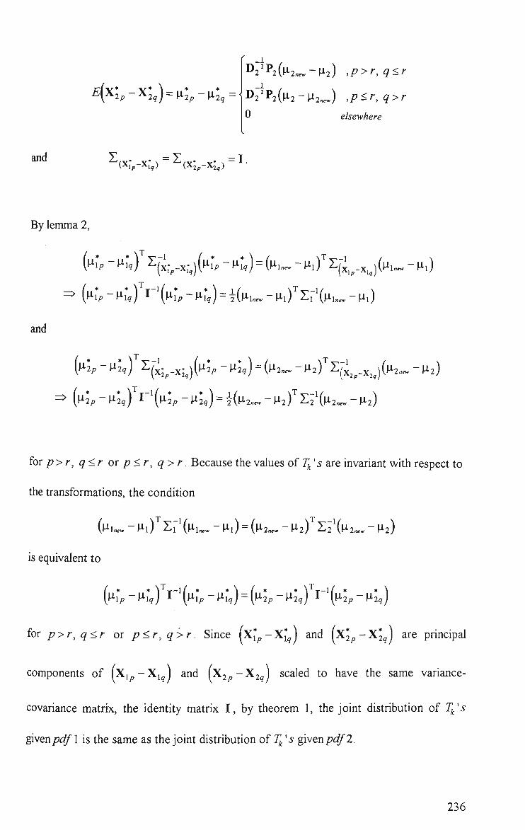
E{Kp-^lq)=U'lp-\ilg =
^?^2{l^2ne.-\^2) ,p>r,q<r
WMP2-li2r^) ,p<r,q>r
0 elsewhere
By lemma 2,
and
(^^^p-^i;,) Z("^.^_^.^) (pr , -P: , )=(PI_-Pi f Z(-^_^_^_^)(Pi.^-PO
> i^ip - \^%)^v\\i\p - p^)=i(pi_ - Pi)'"zrx^iw - \ix)
[\^2p-\^\,) ^("i^-xg(^^2;, -^i2,) = ( i2„ -^X2f 2:(- ^ _ ^ j(p2„ -P2)
for p>r, q<r or p<r, q>r. Because the values of 7 ' 5 are invariant with respect to
the transformations, the condition
(^iw - l^iY Sr C^Aw -^Al) = (P2^. - 2) 2:2X1 2™^ - P2)
is equivalent to
{i^lp-Pig) ^~'(l^%-PU) = {l^lp-l^*2q) ^~^{p*2p-P*2<i)
for p>r, q<r or p<r,q>r. Since (Xi^-XM and (Xj^-Xj^l are principal
components of (Xi^-Xi^j and (X2^-X25) scaled to have the same variance-
covariance matrix, the identity matrix I , by theorem 1, the joint distribution of 7 '5
given pcjj/ l is the same as the joint distribution of 7 '5 given pdf 2.
236

{Q.E.D.)
This theorem can also be adapted to the cases where p is known, namely, if
T v l i (^iw~^l) 5:/(^iw-^i)=(ti2„^-^i) ^~2(p-2ne.-v).
then
/ TkS ,k<r
4x,orX^.) = f ' - ' ,Z, = / r,'54x,orX^.) = P-Ue. ^k>r
1 " ^ 2
M2ne. ,k>r J
The proof for this is along the same line of argument as above except that X, (X, ) and
p,„^ - p,. should be replaced by X^^ - p (X^ - p) and p,„^ - p respectively for / = 1,2.
237

A.2 Dependence of Statistical Performance on X-^,..,.Xp for a Change in
Process Covariance Matrix
Suppose that the process under consideration changes in covariance matrix from
Z to Z„^ after the rth observation, whilst the mean vector p remains constant. It is
shown below that the joint distribution of the 7 '5 (or equivalently, Z^'5) for each of the
control techniques (3.3) to (3.11) depends on p, Z and X„^ through the eigenvalues,
X^,...,X of Z~^Z„e^ or equivalently, of Z„^Z"^
Lemma 4
If Z L 2:r' S L = ^L. ^~2 S L ^ , then there exists a fiiU rank matrix D such that
DZ2D^ = i:i and DZ2„^D^ = Z i „ ^ .
Proof
FromZL Sr^ ^L = slew ^2 S l ^ .we haveZi = [ z L I'lL) I'2[n„^ ^2
Since DZ2 D" = Zi, D = z L S2L • It can easily be verified that D = Z ^ ^ i also
satisfies the equation DZj^ew©^ =2 i„^ . Furthermore, h can readily be seen that
D ^ z L s i i s o f f i i U r a n k .
{Q.E.D.)
.1 ^ T
Inew
238

Theorem 3
Let pdfl be the probabUity density fiinction of the independent multivariate normal
observation vectors X^'s (or X^/5) with mean vector pj , covariance matrix Zi and
^hiew Wore and after the change. Let pdf2 be the probability density fiinction of the
independent multivariate normal observation vectors X^'s (or X^ '5) with mean vector
P2, covariance matrix Z2 and Z2new Wore and after the change. If
z L s r ' S L = S L ^ T-^ i : i _ , then f{T,'s) = f,{T,'s) where f{T,'s) and f(T,'s)
represent the joint distribution of 7^'5 given/^c^ andpdf2 respectively.
Proof
The proof here is similar to that of theorem 1 except that M should be replaced by
D = ZL^ Z 2 L as given in lemma 4.
Theorem 4
If Xj^'s (or X/^'s) are independent random vectors from a multivariate normal
distribution whh constant mean p and a step shift in the covariance matrix from Z to
Z„ew. after the rth observation (or subgroup), then the joint distribution of T/^'s depend
on the eigenvalues of Z~^ Z vf or equivalently, of Z„gvv '^'^ •
Proof
- - I -Theorem 3 implies that the joint distribution of T/^'s depend on Z^^^ Z Z en-- Since
Tj^'s are invariant w.r.t any orthogonal transformation, h is readily seen that Tj^'s
239

^ . - 1 depend on the eigenvalues of Z^^^Z Z^e^. Using the characteristic equation, these
eigenvalues can in turn be shown to be the eigenvalues of Z~^ Z e ,, or T.„ew S~' •
{Q.E.D.)
240

A.3 Dependence of Statistical Performance on n and Q for a Change in Mean
vector and Covariance Matrix
Suppose that the process under consideration changes in mean vector from p to
p„^ and covariance matrix from Z to Z , ^ after the rth observation or subgroup. It is
shown below that the joint distribution of the 7 '5 (or equivalently Z^'s) for each of the
control techniques (3.3)-(3.11) depends on p , p„^, Z and Z„^ through
T = Z~(p„ew-^i)
, which can be interpreted as the vector of noncentrality parameter in the directions of
the principal axes, and the symmetric matrix
_ i - i ^1 = 2~i ^new ^
Theorem 5
Let pdfl be the probability density of the independent multivariate normal observation
vectors X^'s (or X;^'5) with parameters (Pi,Zi) and {\^xnew^^\new) before and after
the change. Let pdfl be the probability density of the independent muhivariate normal
observation vectors X^'s (or X^ ' ) with parameters (P2,5^2) and {P2new^^2new)
before and after the change. If
1 1 _ l —i —-
i:?{Plne.-Pl)^^2'{P2ne.-P2) and ZV^Z.^^IL? ^^?T.,„^^2'
then /,(r,'5) = A(r,'5) where f{T,^s) and f,{T,^s) denote the joint distribution of
r ;5 given pdfl and pdfl respectively. This theorem impUes equivalent performance of
the control techniques under the two ahernative probability densities.
241

Proof
The proof here is similar to that of theorem 2.
242
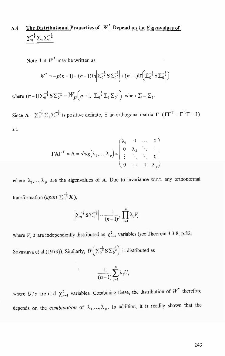
A.4 The Distributional Properties of W* Depend on the Eigenvalues of -I - 1
ZQ Z I Z Q
Note that W may be written as
W* =-p{n-l)-{n-l)lri Zo^SZo^+(«-i)trfZo'sz"^ '0
where {n- l)Zo' S Z ? ~ Wp[n-1, Zo^ Zi Z ? ) when Z = Zj •
T T -TT Since A = ZQ^ DiI^o^ is positive definite, 3 an orthogonal matrix r ( r r = r r = I )
s.t.
FAr" = A = dia^^,...,x)^ =
fA.1 0
0 A.2
0 •••
o\
0 0 X pj
where X^,...,X are the eigenvalues of A. Due to invariance w.r.t. any orthonormal
transformation {upon ILQ^X),
S 2 C V 2 0 "^-^0
1 p -JL_TTx,,^
where V-s are independently distributed as xJ-, variables (see Theorem 3.3.8, p.82,
Srivastava et al.(1979)). Similarly, tr\ Zo ' SZoM is distributed as 1 _ i
("-Dtr
where U^s are i.i.d X«-i variables. Combining these, the distribution of W* therefore
depends on the combination of X„...,Xp. In addition, h is readily shown that the
243
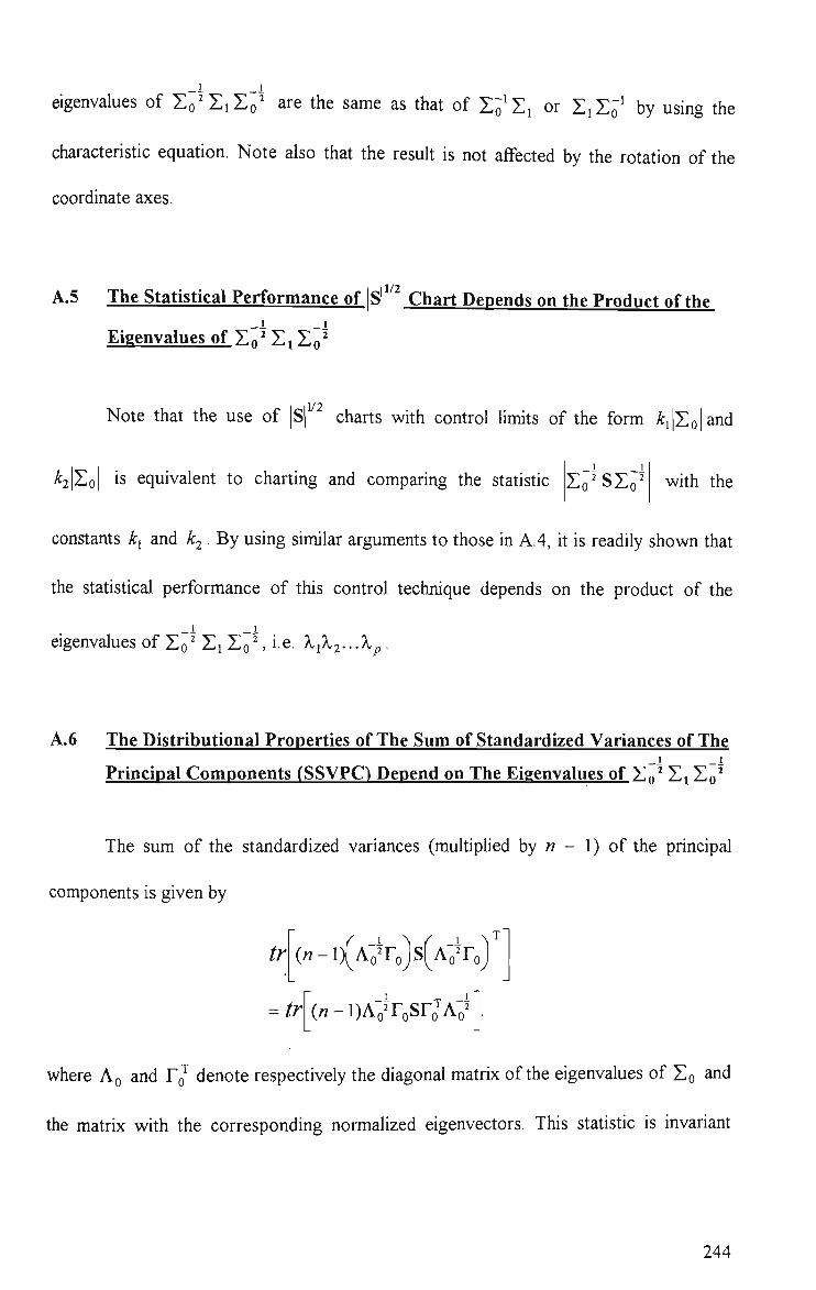
eigenvalues of Z o ' I i Z o ' are the same as that of Zo^Zi or ZiZo' by using the
characteristic equation. Note also that the resuh is not affected by the rotation of the
coordinate axes.
11/2 A.5 The Statistical Performance of |S| Chart Depends on the Product of the
Eigenvalues_of. Z 0 Z1Z 0
|V2 Note that the use of |S| charts with control limits of the form ^i|Zo|and
A:2|Zo| is equivalent to charting and comparing the statistic 2 Zo SZo' whh the
constants k^ and ATJ . By using similar arguments to those in A.4, h is readily shown that
the statistical performance of this control technique depends on the product of the
- 1 _ i
eigenvalues of Zo^ Z I Z Q ^ , ie. X{X2...Xp.
A.6 The Distributional Properties of The Sum of Standardized Variances of The - 1 - 1
Principal Components (SSVPC) Depend on The Eigenvalues of Zq^ Z^ Zp^
The sum of the standardized variances (multiplied by « - 1) of the principal
components is given by
tr (« -1) AoTo S Ao^o
tr («-i)A7roSroX'
where AQ and TQ denote respectively the diagonal matrix of the eigenvalues of ZQ and
the matrix with the corresponding normalized eigenvectors. This statistic is invariant
244
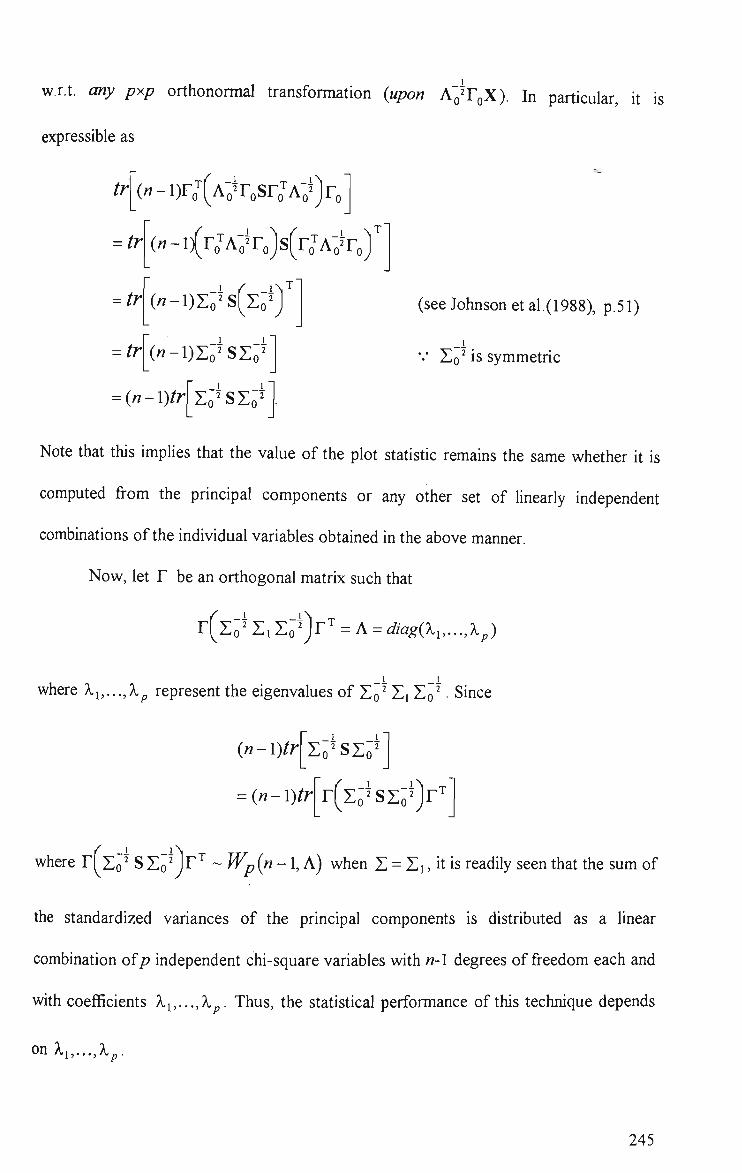
w.r.t. any pxp orthonormal transformation (upon AQ'TQX). In particular, h is
expressible as
tr («-i)roMA7roSroXMro
= tr
= tr
= tr
(« - l ) Fo^Ao^ S F o X ^
(«-l)Zo^S Zo^
(«-l)Z7SZo'
(see Johnson et al.(1988), p.51)
•' ZQ^ is symmetric
= (n-l)tr ZQ S Z Q
Note that this implies that the value of the plot statistic remains the same whether h is
computed from the principal components or any other set of linearly independent
combinations of the individual variables obtained in the above manner.
Now, let F be an orthogonal matrix such that
r{TQ^i:,T~o^r'' = A = diag(x„...,Xp)
where X^,...,Xp represent the eigenvalues of ZQ^ Zi ZQ^ • Since
(n-i)tr Zo SZc
= (n-l)tr r[zo'sZo^)r'
where r[^Zo^ SZQAT'^ ~Wp{n-1, A) when Z = Zi, h is readily seen that the sum of
the standardized variances of the principal components is distributed as a linear
combination of;? independent chi-square variables with n-l degrees of freedom each and
with coefficients Xi,...,Xp. Thus, the statistical performance of this technique depends
onXi,...,X^.
245
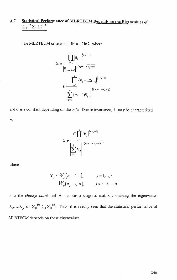
A.7 statistical Performance of MLRTECM Depends on the Eigenvalues of 0 • ^ l • ^ o
The MLRTECM criterion is ^ = -21n ;i where
niS(. i(",-i) _ 1=1
pooled] ij(ni+...+n^-q)
= C—'^
i(",-l)
1
/=1
i;(«/-l)S(,; ("!+•• •+",-9)
and C is a constant depending on the n^'s. Due to invariance, X may be characterized
by
x = —^'-'
\{r-j-l)
| («,+.. .+«^-g) '
where
-Wp{nj-l,A),
j = \--;r
j = r + l,...,q
r is the change point and A denotes a diagonal matrix containing the eigenvalues
Xi,...,X of Zo SiZo • Thus, h is readily seen that the statistical performance of
MLRTECM depends on these eigenvalues.
246

A.8 Scale Invariance of Fisher, Tippett and The Proposed Statistic (Known T.
Case)
Let G = dia^-^,...,-^\ be the diagonal matrix with /th element being the
reciprocal of the standard deviation of the /th variable. The sample covariance matrix
computed from the variables scaled to have unit variances (i.e the sample correlation
matrix) is then given by
S = GSG'
r^ Ar^fs^ s ^ d
d D y
12
>s S,, V~12 ' V
d D '
i;S +d^S , - . , . .22 1 _ _ j2 ' ~12 ~ d ^ f + D S dS^+DS22
V /^c2
'12
^ s ^ + d ^ s „ Y ^ d' ^
v3 « y
- 1 2 / DS
V -12 f 02 / „ 2
DS 22
-~12
d D T
S^al+S^ d M (^iV^i)d'"+S^ DVa, ~ 1 2 ~ / ^ ^~ ~12 /
DS / a i + D S j j d V - 1 2 / ~
DS„D 22 J
~12 / DS la, DS22D^
- 1 2 / ^
(seep.591, Anderson(1984))
where d denotes the zero vector of (p-l) elements, S22 is the sample covariance
matrix of the last (p-l) variables, D = ^ J ' « ^ ^ > " M ^ ] and
S" = (7 i2 i'S'2 RuS.Sj • • • RipS^Sp). Similarly, the population correlation matrix is ~12 ^
Z =GZG^
^ 1 ^Z[2D"^ Oi
i D Z i 2 0X22 D'
247
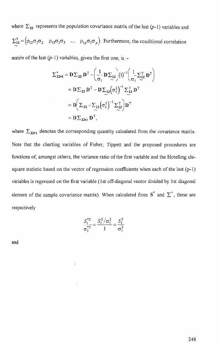
where Z22 represents the population covariance matrix of the last (p-l) variables and
I12 = (pi2 iCf2 Pi3 i< 3 • • • Pip^i^p) • Furthermore, the conditional correlation
matrix of the last (p-l) variables, given the first one, is :-
i:;2.i - 01:22 D^-f—DzJ(irf-xLD''
= DZ22 D"" - I>2i2(c7f ) ' ^J2 D""
^22-212(^0"'^J^ID" = D
where Z22.1 denotes the corresponding quantity calculated from the covariance matrix.
Note that the charting variables of Fisher, Tippett and the proposed procedures are
flinctions of, amongst others, the variance ratio of the first variable and the HoteUing chi-
square statistic based on the vector of regression coefficients when each of the last (p-l)
variables is regressed on the first variable (1st off-diagonal vector divided by 1st diagonal
element of the sample covariance matrix). When calculated from S and Z , these are
respectively
2 / _ 2
o? 1 "a?
and
248

/ s ~12
*T / \
*2 r. -1 r^*
22>1
V(n-l)SiV
1 V T TkTA :^S^D^ i S i 2 D ^ D l 2 2 . i D ' " ^ " '
/• fDS
12 oi
DZ 12
2 / _ 2 ^1 / a i
i.e their values remain the same whether they are calculated from the original or
standardized variables. Note also that the other statistics incorporated into the charting
variables are obtained from S _ i..._y_i and Zy,...,p.i,...j_i (/ = 2,...,p) in exactly the
same manner. Thus, to complete the proof, h is only required to show that S ^^i ._ _i
and Z* ...,p.i,.,.j-i are of the same form as S* and Z* • For this, let
G = G i l ^ 1 2
^ ^ 2 1 ^ 2 2 ^ and S =
S i i Si2
,821 s 22>
where Gu and Sn denotes the ( y - l ) x ( 7 - l ) submatrices. Note that G12 here
represents the (7 -1) x (/> - 7 +1) zero matrix. Thus,
S =GSG' = 22 ^^11^11^11 G11S12G
VG22S21G11 G22S22G22>'
and
S;,.„,.i....,;-i = G22S22GI2 -(G22S2iG[i)(GnSHG;^i)'^(GHSi2Gl2)
= G22S22GI2 -G22S2iGi\(G?-,)"'sr;Gr/G„S,2GL
= G22S22G22 -G22S21S11S12G22
= 022^822 -S21S11S12JG2
= G22Sy^...^p.l^..^y_lG22
.T ^22
249

* T
which is clearly of the same form as S = GSG . Likewise, h can be shown that
Z* ...,p.i,...j-i is of the same form as Z* •
A.9 Scale Invariance of Fisher, Tippett and The Proposed Statistic (Unknown
Z Case)
The proof here is similar to those in A.8.
250
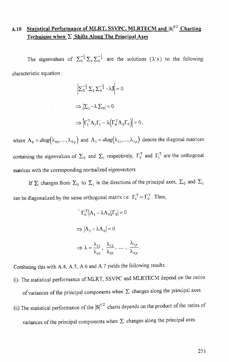
II1/2 A.10 Statistical Performance of MLRT, SSVPC, MLRTECM and |S| Charting Technique when Z Shifts Along The Principal Axes
The eigenvalues of Zo^EiZo^ are the solutions (Vs) to the following
characteristic equation
Zo^ ZiZo^ ~^I
=>|Zi-?.Zo| = o
= 0
z^|rXri-^(roXro)| = o,
where AQ=diag{XQi,...,XQp) and Ai=diag{x^^,...,Xip) denote the diagonal matrices
containing the eigenvalues of ZQ and Zi respectively, TJ and T^ are the orthogonal
matrices with the corresponding normalized eigenvectors.
If Z changes from ZQ to Zi in the directions of the principal axes, ZQ and Zi
T T-T can be diagonaUzed by the same orthogonal matrix i.e. Fi = FQ . Thus
Ai-^Ao||ro| = 0
|Ai-A,Ao| = 0
X = ^11 ^12
A,oi A-
-lp
, . . . , X Op
Combining this with A.4, A.5, A.6 and A.7 yields the foUowing resuhs :
(i) The statistical performance of MLRT, SSVPC and MLRTECM depend on the ratios
of variances of the principal components when Z changes along the principal axes,
(ii) The statistical performance of the |sf ^ charts depends on the product of the ratios of
variances of the principal components when Z changes along the principal axes.
251
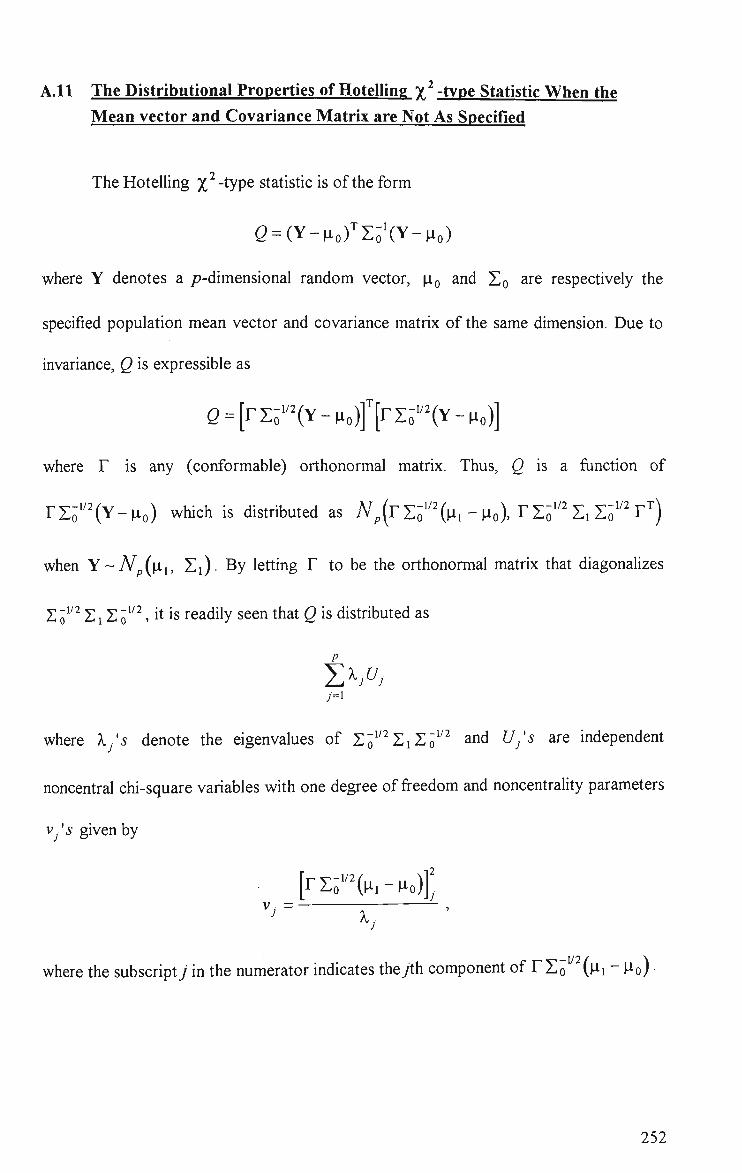
A.11 The Distributional Properties of Hotelling Y^ -type Statistic When the Mean vector and Covariance Matrix are Not As Specified
The HoteUing X^-type statistic is of the form
G- (Y-Po) ' 'Zo ' (Y-Po)
where Y denotes a /7-dimensional random vector, pg and ZQ are respectively the
specified population mean vector and covariance matrix of the same dimension. Due to
invariance, Q is expressible as
e = [^Ii• '^(Y-^^„)f[^Ii"^(Y-^.„)]
where F is any (conformable) orthonormal matrix. Thus, Q is a function of
rZo^ ' (Y-po) which is distributed as A^^(rZo'''(Pi - Po), FZo'^'Zj Zo''^ F^)
when Y ~Np{iii, Zi) . By letting F to be the orthonormal matrix that diagonaUzes
2 0^ Z1Z 0 ^ , h is readily seen that Q is distributed as
where X/s denote the eigenvalues of ZQ^^^ZIZQ^'^ and U/s are independent
noncentral chi-square variables whh one degree of freedom and noncentrality parameters
vfs given by
. [rZ5"^(n,-n„)]; ^ = X, •
where the subscript^ in the numerator indicates the7th component of F ZQ {\^\ - J o)
252

Simulation Programs
253
"PR0G1"<-function(p, r, m, X, noiter)
{ jmmmmmmimwmmmmmmmitiiiiiiiiiiiiiiiiiiffititif^ # This program, which is written in Spins, simulates the probabiUties of detecting a sustained shift in # # the mean vector within m observations by the multivariate control charts (3.3), (3.4), (3.5) and (3.6). # # Only upper control limit is used. This is set at 0.27% level of significance, p - dimension, r - change # # point, X - noncentrality parameter, noiter - number of replications. #
noobs <- r + m resultl <- 0 result2 <- 0 result3 <- 0 result4 <- 0 stat3sing <- 0 stat4sing <- 0 tempi <- rep(0,p) temp2 <- c(A, ,rep(0,p-l)) temp3 <- diag(p) for(iin 1: noiter) {
samp <- rbind(GENERATE(templ,temp3, r), GENERATE(temp2,temp3,m)) meanvec2 <- apply(samp[(l:r), ], 2, mean) meanvec4 <- meanvec2 covmat4<-var(samp[(l:r), ]) devmat3 <- samp - matrix(templ, noobs, p, T) sumcrspd3 <- matrix(0, p, p) for(ginl:r){
sumcrspd3 <- sumcrspd3 + outer(devmat3[g, ], devmat3[g, ]) } j <- r + 1 repeat {
statl <- sampD, ] %*% sampO, ] statl <- pchisq(statl, p) if(statl >= 0.9973) {
resultl <- resultl + 1 break
} j<- j + l if(j > noobs)
break }
j <- r + 1 repeat {
stat2 <- ((j - l)/j) * (samp[j, ] - meanvec2) %*% (sampO, 1 - meanvec2) stat2 <- pchisq(stat2, p) if((stat2>= 0.9973)) {-
resultZ <- result2 + 1 break
meanvec2 <- {(Q -1) * meanvec2) + samp[j, ])/j
if(j > noobs) { break
} } j <- r + 1 repeat {
254

if (qr(sumcrspd3)$rank < p){ stat3sing <- stat3sing + 1 break
} stat3 <- (((j - p) * (j - l))/(p * (j -1))) * devmat3[j, ] %*% solve(sumcrspd3) %*%
devmat3[j, ] stat3 <- pf(stat3, p, j - p) if(stat3 >= 0.9973) {
results <- results + 1 break
} sumcrspd3 <- sumcrspd3 + outer(devmat3[j, ], devmat3[j, ]) j < - j + l if(j > noobs){
break }
} j <- r + 1 repeat {
if (qr(covmat4)$rank < p){ stat4sing <- stat4sing + 1 break
} stat4 <- (((j - 1 - P) * (j - !))/(] * (j - 2) * p)) * (samplj, ] - meanvec4) %*%
solve(covmat4) %*% (samp[j, ] - meanvec4) stat4 <- pf(stat4, p, j - 1 - p) if(stat4 >= 0.9973){
result4 <- result4 + l break
} meanvec4 <- (((j -1) * meanvec4) + samp[j, ])/j covmat4 <-var(samp[(l:j), ]) j < - j + l if(j > noobs) {
break }
} results <- results / (noiter - statSsing) result4 <- result4 / (noiter - stat4sing) c(resuhl,result2,resultS,result4)
255

"PR0G2"<-function(p, n, r, m, X, noiter)
{
# This program, which is written in Spins, simulates the probabilities of detecting a sustained shift in # # the mean vector within m subgroups of size n each by the multivariate control charts (3.7), (3.8), # # (3.9), (3.10) and (3.11). Only upper control limit is used. This is set at 0.27% level of significance. # #/7-dimension. A--change point, X - noncentrality parameter, no/7er-number of replications. #
nosub <- r + m resultl <- 0 result2 <- 0 results <- 0 result4 <- 0 results <- 0 StatSsing <- 0 stat4sing <- 0 StatSsing <- 0 tempi <- rep(0,p) temp2 <- c( X ,rep(0,p-l)) tempS <- diag(p) temp4 <- matrix(0,p,p) for(i in 1: noiter) {
samp <- rbind(GENERATE(templ, tempS, r*n), GENERATE(temp2, tempS, m*n)) sumcrspd3 <- crossprod(samp[(l:(n * r)), ], samp[(l:(n * r)), ]) meanvec2 <- apply(samp[l:(n * r), ], 2, mean) meanvecS <- meanvec2 covS <- temp4 fo r (g in l : ( r+ l ) ){
covS <- covS + var(samp[(((g -1) * n) + l):(g * n), ])
} covS <- cov5/(n +1) cov4 <- covS j <- r + 1 repeat {
statl <- n * apply(samp[(((j -1) * n) + 1):CJ * n), ], 2,mean) %*% apply(samp[(((j -1) * n) + l):(j * n), ], 2, mean)
if(statl >= qchisq(0.9973,p)) { resultl <- resultl + 1 break
} j < - j + l if(j > nosub) {
break
} } j <- r + 1 repeat {
stat2 <- (n/j) * (j -1) * (apply(samp[(((j -1) * n) + l):(j * n), ], 2, mean) -meanvec2) %*% (apply(samp[((a -1) * n) + l):(j * n), ], 2, mean) -meanvec2)
if(stat2 >= qchisq(0,9973,p)) { result2 <- result2 + 1 break
} j < - j + l if(j > nosub) {
256

break
} meanvec2 <- (((j - 2) * meanvec2) + apply(samp[(((j - 2) * n) + l):((j -1) *
n), ], 2, mean))/(j -1) } j <- r + 1 repeat {
if( qr(sumcrspdS)$rank < p){ StatSsing <- statSsing + 1 break
} stat3 <- (n/p) * (n * (j -1) - p + 1) * apply(samp[((0 -1) * n) + 1):G * n), ],
2, mean) %*% solve(sumcrspd3) %*% apply(samp[(((j - 1) * n) +l):(j * n), ], 2, mean)
if(statS >= qf(0.997S, p, n * (j-l) - P + 1)) { results <- results + 1 break
> j < - j + l if(i > nosub) {
break } sumcrspdS <- sumcrspdS + crossprod(samp[(((j - 2) * n) + l):((j -1) * n), ],
samp[(((j - 2) * n) + l):((j -1) * n), ]) } j <- r + 1 repeat {
if( qr(cov4)$rank < p ){ stat4sing <- stat4sing + 1 break
} stat4 <- (n/(p * j * (n - 1))) * (0 * (n -1)) - p + 1) * apply(samp[(((j - 1) * n)
+ l):(j * n), ], 2, mean) %*% solve(cov4) %*% apply(samp[(((j -1) * n) + l):(j * n), ], 2, mean)
if(stat4 >= qf(0.997S, p, (j * (n - 1)) - P + 1)){ result4 <- result4 + 1 break
} j < - j + l if(j > nosub) {
break } cov4 <- ( ( j - l ) * cov4 + var(samp[((0 -1) * n) + l):(j * n), ]))/j
} j <- r + 1 repeat {
if( qr(cov5)$rank < p){ StatSsing <- statSsing + 1 break
stats <- (n/(j * j * P * (n -1))) * 0 -1) * (C * (n -1)) - P + D * (apply(samp[((0 -1) * n) + l):a * n), ], 2, mean) - meanvecS) %*% solve(covS) %*% (apply(samp[((a -1) * n) + l):(j * n), ], 2, mean) -meanvecS)
if(statS >= qf(0.9973, p, j * (n -1) - p + 1)){ results <- results + 1 break
}
257

j<- j + l if(j > nosub) {
break } meanvecS <- ((0 - 2) * n * meanvecS) + apply(samp[(((j - 2) * n) + l):((j -1)
* n), 1, 2, sum))/((i -1) * n) covS <- ((0 -1) * covS) + var(samp[(((j -1) * n) + l):(j * n), ]))/j
} } resultl <- resultl / noiter result2 <- result2 / noiter results <- results / (noiter - stat3sing) result4 <- result4 / (noiter - stat4sing) resuhs <- results / (noiter - statSsing) c(resultl,result2,result3,result4,resultS)
258

"PR0G3"<-fimction(p, y , h, d, r, k, noiter, a , X^g„^)
{
mmitiiiiiiiiiiitmmmmimmimmmMmiiiiiiiiiiiiiiiiiiHiummmmfifimiii^^ #This program, which is written in Splus, simulates the n/w length probabilities of EWMAZl, # # EWMAZ2, EWMAZS and M chart for a linear trend, p - dimension, y - EWMA smoothing constant # #h- control chart factor of EWMA, d - moving sample size for M chart,r - change point, : - maximum # # run length for which the probability is simulated, noiter- number of iterations, a - significance level # # used with the M chart, X,f^g„^-trend parameter. # #4^^ifimmmmmmimmmmmmmfiiiiiiiiiiiiiiiiiiititim
if(p = 2){ a<-2
} else {
a <- ceiling((3 * (p -1) + sqrt((p -1) * (9 * p -17)))/4) } EWMAZ IRL <- numeric(k) MRL <- numeric(k) EWMAZ2RL <- numeric(k) EWMAZSRL <- numeric(k) EWMAZ ICP <- numeric(k) MCP <- numeric(k) EWMAZ2CP <- numeric(k) EWMAZS CP <- numeric(k) EWMAZl sing <- 0 Msing <- 0 EWMAZ2sing <- 0 EWMAZS sing <- 0 temp <- matrix(0, p, p, T) tempi <- matrix(seq(l, k), k, p, F) * matrix(c( A, g„ , rep(0, p -1)), k, p, T) temp2 <- h * sqrt( y /(2 - y )) temp3 <- k + r - a -1 temp4 <- qf(l - a , p, d - p) tempS <- k + r - d + 1 temp6 <- r + 2 - d for(i in 1 inciter) {
cov <- temp samp <- rbind(GENERATE(rep(0, p), diag(p), r), GENERATE(rep(0, p), diag(p), k)
+ tempi) for(gin l:a) {
cov <- cov + outer(samp[g + 1, ] - samp[g, ], samp[g +1, ] - samp[g, ]) } EWMAZl <- 0 if((a + 2)>r){
j < - l . repeat {
if(qr(cov)$rank < p) { EWMAZl sing <- EWMAZl sing + 1 break
} f <- (2 * ((j + a - 1) 2))/(S * (j + a) - 4) Z K - ((f - p + 1) * (3 * (j + a) - 4) * (sampD + a + 1, ]) %*%
solve(cov) %*% (sampLJ + a + 1, l))/(p * (j + a -D)
ZI <- qnorm(pf(Zl, p, f - p + 1), 0, 1) EWMAZl <- y * ZI + (1 - y ) * EWMAZl
259
if(abs(EWMAZl) > temp2) { EWMAZlRL[j + a + 1 - r] <-EWMAZlRLO + a + 1 - r] +1 break
} cov <- cov + outer(samp[j + a + 1, ] - sampO + a, ], sampO + a + 1,
] - sampO + a, ]) j<- j + l if(j > tempS) { break
} >
} else if((a + 2) < r) {
Zlflag <- 0 for(jin l:(r-a-1)) {
if(qr(cov)$rank < p) { EWMAZlsing <- EWMAZlsing + 1 Zlflag <-1 break
} f <- (2 * ((j + a -1)''2))/(3 * (j + a) - 4) Zl<- ((f - p + 1) * (3 * (j + a) - 4) * (samp[j + a + 1, ]) %*%
solve(cov) %*% (sampO + a + 1, ]))/(p * (j + a -D)
ZI <- qnorm(pf(Zl, p, f - p + 1), 0, 1) EWMAZl <- y * ZI + (1 - y ) * EWMAZl cov <- cov + outer(sampD + a + 1, ] - samp[j + a, ], samp[j + a + 1,
] - samplj + a, ]) } if(Zlflag == 0) {
j <- r - a repeat {
if(qr(cov)$rank < p) { EWMAZlsing <- EWMAZlsing + 1 break
} f <- (2 * ((j + a - 2)^2))/(3 * (j + a) - 4) Zl<- ((f - p + 1) * (3 * (j + a) - 4) * (samp[i + a + 1, ]) %*%
solve(cov) %*% (sampD + a + 1, ]))/(p * C + a -1)) ZI <- qnorm(pf(Zl, p, f - p + 1), 0, 1) EWMAZl <- y * ZI + (1 - y ) * EWMAZl if(abs(EWMAZl) > temp2) { EWMAZIRLD - r + a + 1] <-EWMAZIRLO - r + a + 1] + 1 break
:COV <- cov + outer(sampO + a + 1, 1 - samp[j + a, ], samp[j + a + l,]-sampO + a, ])
j< - j + l if(j > tempS) { -' break }
} }
} else {
if(qr(cov)$rank >= p) { f<-(2*(a'^2))/(3*a-l)
260

Z K - ((f - p + 1) * (3 * a -1) * samp[a + 2, ] %*% solve(cov) %*% samp[a + 2, ])/(p * a)
ZI <- qnorm(pf(Zl, p, f - p + 1), 0, 1) EWMAZl <- Y * ZI + (1 - y ) * EWMAZl
cov <- cov + outer(samp[a + 2, ] - samp[a +1,], samp[a + 2, ] -samp[a+ 1, ])
j < - l repeat {
if(qr(cov)$rank < p) { EWMAZlsing <- EWMAZlsing + 1 break
} f<- (2*(G + a)^2))/(3*0 + a ) - l ) Z K - ((f - p + 1) * (3 * 0 + a) -1) * samp[j + a + 2, ] %*%
solve(cov) %*% samp[j + a + 2, ])/(p * (j + a)) ZI <- qnorm(pf(Zl, p, f - p + 1), 0, 1) EWMAZl <- y * ZI + (1 - y ) * EWMAZl if(abs(EWMAZl) > temp2) {
EWMAZIRLO] <- EWMAZlRL[j] + 1 break
} cov <- cov + outer(samp[j + a + 2, ] - samp[j + a + 1, ], samp[j + a
+ 2, ]-sampD + a + l , ])
j < - j + l if(j > k) {
break }
} } else {
} } i f (d>r){
j < - l repeat {
EWMAZlsing <- EWMAZlsing + 1
X <- samp[(j:0' + d -1)). I w <- seqO, j + d -1) - rep((2 * j + d -1)/2, d) z <- (t(x) %*% w)/sqrt(as.numeric(w %*% w)) M <- t(x) %*% X if(qr(M)$rank >= p) {
M <- t(solve(M) %*% z) %*% z M <- M/(l - M) if(M > temp4) {
MRLIj + d -1 - r] <- MRL[j + d -1 - r] + 1 . break
} j < - j + l if(j > tempS) {
break
} } else {
Msing <- Msing + 1 break
>
261
} else {
j <- temp6 repeat {
x<-samp[a:a + d - l ) ) , ] w <- seqO, j + d -1) - rep((2 * j + d -1)/2, d) z <- (t(x) %*% w)/sqrt(as.numeric(w %*% w)) M <- t(x) %*% X if(qr(M)$rank >= p) {
M <- t(solve(M) %*% z) %*% z M <- My(l - M) if(M > temp4) {
MRLIj + d -1 - r] <- MRL[j + d -1 - r] + 1 break
} j <-J + 1 if(j > tempS) { break
} } else {
Msing <- Msing + 1 break
} }
} if((p + 1) <= r) {
EWMAZ2 <- 0 Z2flag <- 0 for(j in (p + l):r) {
Z2 <- apply(samp[(l:(j -1)), ], 2, mean) w <- ((j - 2)/(j -1)) * var(samp[(l:(j -1)), ]) + outer(Z2, Z2) if(qr(w)$rank < p) {
Z2flag <-1 EWMAZ2sing <- EWMAZ2sing + 1 break
} Z2 <- (G - p) * sampO, ] %*% solve(w) %*% samp[j, ])/(p *Q-l)) ZI <- qnorm(pf(Z2, p, j - p), 0, 1) EWMAZ2 <- y * Z2 + (1 - y ) * EWMAZ2
} if(Z2flag == 0) {
j <- r + 1 repeat {
Z2 <- apply(samp[(l:(j -1)), ], 2, mean) w <- (0 - 2)/(j - 1)) * var(samp[(l:(j -1)), ]) + outer(Z2, Z2)
'if(qr(w)$rank < p) { EWMAZ2sing <- EWMAZ2sing + 1 break
} Z2 <- ((j - p) * sampO, ] %*% solve(w) %*% samp[j, ])/(p * (j -
D) Z2 <- qnorm(pf(Z2, p, j - p), 0, 1) EWMAZ2 <- y * Z2 + (1 - y ) * EWMAZ2
if(abs(EWMAZ2) > temp2) { EWMAZ2RL[j - r] <- EWMAZ2RL[j - r] + 1 break
262

} j < - j + l if(j>(r + k)){
break }
} }
} else {
EWMAZl <- 0 j < - p + l repeat {
Z2 <- apply (samp [(l:(j -1)), ], 2, mean) w <- ((j - 2)/0 - 1)) * var(samp[(l:(j -1)), ]) + outer(Z2, Z2) if(qr(w)$rank < p) {
EWMAZ2sing <- EWMAZ2sing + 1 break
} Z2 <- ((j - p) * sampLj, ] %*% solve(w) %*% samp[j, ])/(p * (j -1)) Z2 <- qnorm(pf(Z2, p, j - p), 0, 1) EWMAZ2 <- y * Z2 + (1 - y ) * EWMAZ2
if(abs(EWMAZ2) > temp2) { EWMAZ2RLIJ - r] <- EWMAZ2RL[j - r] + 1 break
} j < - j + l if(j>r + k){
break }
} } if((p + 2) <= r) {
EWMAZS <- 0 ZSflag <- 0 for(j in (p + 2):r) {
w<-var(samp[(l:(j-l)), ]) if(qr(w)$rank < p) {
EWMAZSsing <- EWMAZSsing + 1 ZSflag <-1 break
} ZS <- (CJ - P - 1) * sampD, ] %*% solve(w) %*% samp[j, ])/(p * 0 -
2)) ZS <- qnorm(pf(Z3, p, j - p -1), 0, 1) EWMAZS <- y * ZS + (1 - y ) * E W M A Z S
} :. if(ZSflag = 0) {
j <- r + 1 repeat {
w<-var(samp[(l:(j -1)), 1) if(qr(w)$rank < p) {
EWMAZSsing <- EWMAZSsing + 1 break
ZS <- ((j - p -1) * sampO, ] %*% solve(w) %*% sampLj, ])/(p * (j
-2)) ZS <- qnorm(pf(Z3, p, J - p -1), 0,1)
263
EWMAZS <- y * ZS + (1 - y ) * EWMAZS
if(abs(EWMAZS) > temp2) { EWMAZ3RL[j - r] <- EWMAZ3RL[j - r] + 1 break
} j < - j + l i fa>(k + r)){ break
} }
} else {
EWMAZS <- 0 j < - p + 2 repeat {
w<-var(samp[(l:(j-l)), ]) if(qr(w)$rank < p) {
EWMAZSsing <- EWMAZSsing + 1 break
} ZS <- ((j - p -1) * samplj, ] %*% solve(w) %*% samp[j, ])/(p * (j
2)) ZS <- qnorm(pf(Z3, p, j - p -1), 0, 1) EWMAZS <- y * ZS + (1 - y ) * EWMAZS if(abs(EWMAZ3) > temp2) {
EWMAZSRL[j - r] <- EWMAZSRL|j - r] + 1 break
}
j <-J + 1 if(j>(k + r)){ break
} }
} } for(iinl:k){
EWMAZlCP[i] <- sum(EWMAZlRL[l:i])/(noiter - EWMAZlsing) MCP[i] <- sum(MRL[l:i])/(noiter - Msing) EWMAZ2CP[i] <- sum(EWMAZ2RL[l:i])/(noiter - EWMAZ2sing) EWMAZ3CP[i] <- sum(EWMAZ3RL[l:i])/(noiter - EWMAZSsing)
} results <- maUix(c(EWMAZlCP, MCP, EWMAZ2CP, EWMAZSCP), k, 4, F) if((r==l)&&(A-^,„^==0)){
results <- rbind(rep(0,4),results[(l:(k-l)),])
} results
264

"PR0G4"<-function(p, y , h, d, r, k, noiter, a , Xf^^„j)
{
if^MumwuummmmmmMiiiiiiiiiiififmiiiiiiiiiiiiiiiiiiiiiiiiiiiiiiiiiiiiii^^ # This program, which is written in Splus, simulates the run length probabilities of EWMAZIU, # #EWMAZ2U, MCHARTU for a linear trend. /?-dimension, y -EWMA smoothing constant, # # h - control chart factor of EWMA, d - moving sample size for MCHARTU, r - change point, k - max # # run length for which the probability is simulated, noiter- number of iterations, a - significance level # # used with the MCHARTU, X ^ ^ - trend parameter. #
##################################i///////////////////////####M#^^ if(p = 2){
a < - 2
} else {
a <- ceiling((S * (p -1) + sqrt((p -1) * (9 * p -17)))/4)
} EWMAZlURL <- numeric(k) MURL <- numeric(k) EWMAZ2URL <- numeric(k) EWMAZlUCP <- numeric(k) MUCP <- numeric(k) EWMAZ2UCP <- numeric(k) EWMAZlUsing <- 0 MUsing <- 0 EWMAZ2Using <- 0 tempi <- matrix(0, p, p, T) temp2 <- matrix(seq(l, k), k, p, F) * mattix(c( X^^^^^, rep(0, p -1)
), k, p, T) tempS <- h * sqrt(y /(2 - y ))
temp4 <-k + r - a - l temps <- qf(l - a , p, d - p -1) temp6 <- k + r - d + 1 temp7 <- r + 2 - d for(iin 1: noiter) {
cov <- tempi samp <- rbind(GENERATE(rep(0, p), diag(p), r), GENERATE(rep(0, p), diag(p), k)
+ temp2) meanvec <- apply(samp[(l:(a + 1)), ], 2, mean) for(gin l:a) {
cov <- cov + outer(samp[g + 1, ] - samp[g, ], samp[g + 1, ] - samp[g, ])
} EWMAZIU <- 0 if((a + 2) > r) {
j < - l repeat {
if(qr(cov)$rank < p) { EWMAZlUsing <- EWMAZlUsing + 1 break
} f <- (2 * ((j + a -1)^2))/(3 * (j + a) - 4) ZIU <- ((j + a) * (f - p + 1) * (3 * (j + a) - 4) * (sampO + a + 1, ] -
meanvec) %*% solve(cov) %*% (sampD + a + 1, ] -meanvec))/(p * (j + a -1) * (j + a + 1))
ZIU <- qnorm(pf(ZlU, p, f - p + 1), 0, 1) EWMAZIU <- y * ZIU + (1 - y ) * E W M A Z I U
if(abs(EWMAZlU) > tempS) {
265

EWMAZlURL[j + a + 1 - r] <- EWMAZlURL[j + a + 1 - r] + 1 break
} meanvec <- apply(samp[(l:(j + a + 1)), ], 2, mean) cov <- cov + outer(samp[j + a + 1, 1 - samp[j + a, ], sampO + a + 1,
]-sampO + a, ]) j < - j + l if(j > temp4) {
break
} }
} else if((a + 2) < r) {
j < - l while((j <= (r - a - 1)) && (qr(cov)$rank >= p)) {
f <-(2 * (0 + a -1)^2))/(3 * (j + a) - 4) ZIU <- (0 + a) * (f - p + 1) * (3 * a + a) - 4) * (samp[j + a + 1, ] -
meanvec) %*% solve(cov) %*% (samp[j + a + 1, ] -meanvec))/(p * (j + a -1) * 0 + a + 1))
ZIU <- qnorm(pf(ZlU, p, f - p + 1), 0, 1) EWMAZIU <- y * ZIU + (1 - y ) * EWMAZIU meanvec <- apply(samp[(l:Cj + a + 1)), ], 2, mean) cov <- cov + outer(samp[j + a + 1, ] - sampjj + a, ], samp[j + a + 1,
] - samplj + a, ]) j <-J + 1
} if(j = (r - a)) {
repeat { if(qr(cov)$rank < p) {
EWMAZlUsing <- EWMAZlUsing + 1 break
} f <- (2 * ((j + a - l)'^2))/(3 * (j + a) - 4) ZIU <- ((j + a) * (f - p + 1) * (3 * (j + a) - 4) * (sampD + a + 1, ] -
meanvec) %*% solve(cov) %*% (samp[j + a + 1, ] -meanvec))/(p * (j + a -1) * 0 + a + 1))
ZIU <- qnorm(pf(ZlU, p, f - p + 1), 0, 1) EWMAZIU <- y * ZIU + (1 - y ) * E W M A Z I U
if(abs(EWMAZlU) > tempS) { EWMAZIURLD + a + 1 - r] <- EWMAZlURL[j + a + 1 - r] + 1 break
meanvec <- apply(samp[(l:(i + a + 1)), ], 2, mean) cov <- cov + outer(samp[j + a + 1, ] - sampQ + a, ],samp[j + a +
1, ] - sampU + a, ])
J <-J + 1 if(j > temp4) {
break
} }
} else {
EWMAZlUsing <- EWMAZlUsing + 1
} } else {
if(qr(cov)$rank >= p) {
266
f< - (2* (a^2 ) ) / (3*a - l ) Z l U < - ( ( a + l ) * ( f - p + l ) * ( 3 *a - l )* ( samp[a + 2, ] -
meanvec) %*% solve(cov) %*% (samp[a + 2, ] -meanvec))/(p * a * (a + 2))
ZIU <- qnorm(pf(ZlU, p, f - p + 1), 0, 1) EWMAZIU <- y * ZIU + (1 - y ) * EWMAZIU
meanvec <- apply(samp[(l:(a + 2)), ], 2, mean) cov <- cov + outer(samp[a + 2, ] - samp[a + 1,], samp[a + 2, ] -
samp[a + 1, ])
j < - l repeat {
if(qr(cov)$rank < p) { EWMAZlUsing <- EWMAZlUsing + 1 break
} f <- (2 * ((i + a)^2))/(S * (j + a) -1) ZIU <- ((j + a + 1) * (f - p + 1) • (3 * 0 +a) -1) * (samp[j + a + 2,
] - meanvec) %*% solve(cov) %*% (samplj + a + 2, ] -meanvec))/(p * (j + a) * (j + a + 2))
ZIU <- qnorm(pf(ZlU, p, f - p + 1), 0, 1) EWMAZIU <- y * ZIU + (1 - y ) * EWMAZIU
if(abs(EWMAZlU) > tempS) { EWMAZlURLIj] <- EWMAZlURL[j] + 1 break
} meanvec <- apply(samp[(l:(j + a + 2)), ], 2, mean) cov <- cov + outer(samp[j + a + 2, ] - samp[j + a + 1, ], sampjj + a
+ 2, ] - samplj + a + 1, ]) j <-J + 1 ifO>k){
break }
} } else {
} } i f (d>r){
j < - l repeat {
EWMAZlUsing <- EWMAZlUsing + 1
X <- samp[(j:(j + d -1)), ] - matrix(apply(samp[(j:(j + d -1)), ], 2, mean), d, p, T)
w <- seq(j, j + d -1) - rep((2 * j + d -1)/2, d) z <- (t(x) %*% w)/sqrt(as.numeric(w %*% w)) MU <- t(x) %*% X if(qr(MU)$rank >= p) {
MU <- t(solve(MU) %*% z) %*% z MU <- MU/(1 - MU) if(MU > tempS) {
MURL[j + d -1 - r] <- MURL[j + d -1 - r] + 1 break
} j < - j + l if(j > temp6) {
break >
267

} else {
MUsing <- MUsing + 1 break
} }
} else {
j <- temp7 repeat {
X <- samp[(j:(j + d -1)), ] - mattix(apply(samp[(j:(j + d -1)), ], 2, mean), d, p, T)
w <- seq(j, j + d - 1) - rep((2 * j + d -1)/2, d) z <- (t(x) %*% w)/sqrt(as.numeric(w %*% w)) MU <- t(x) %*% x if(qr(MU)$rank >= p) {
MU <- t(solve(MU) %*% z) %*% z MU <- MU/(1 - MU) if(MU > tempS) {
MURLIj + d -1 - r] <- MURL|j + d - 1 - r] +1 break
} j < - j + l if(j > temp6) { break
} } else { MUsing <- MUsing + 1 break
} }
} if((p + 2) <= r) {
EWMAZ2U <- 0 j < - p + 2 repeat {
Z2U <- apply(samp[(l:(j -1)), ], 2, mean) w <- var(samp[(l:(j -1)), ]) if(qr(w)$rank >= p) {
Z2U <- ((i -1) * (j - P -1) * (samplj, ] - ZIU) %*% solve(w) %*% (sampD, ] -Z2U)) /a*P*( j -2 ) )
Z2U <- qnorm(pf(Z2U, p, j - p - 1), 0, 1) EWMAZ2U <- y * Z2U + (1 - y ) * EWMAZ2U j < . j + l ,ifG > r) { ' break
} } else {
EWMAZ2Using <- EWMAZ2Using + 1 break
} } i fO==( r+ l ) ){
repeat { Z2U <- apply(samp[(l:0 -1)), ], 2, mean)
268

w<-var(samp[(l:(j-l)), ]) if(qr(w)$rank < p) {
EWMAZ2Using <- EWMAZ2Using + 1 break
} Z2U <- (0 -1) * (j - P -1) * (samp[j, ] - Z2U) %*% solve(w) %*%
(samplj, ] -Z2U)) / ( j*p*a-2) ) Z2U <- qnorm(pf(Z2U, p, j - p -1), 0, 1) EWMAZ2U<-y * Z2U + (1 - y ) * EWMAZ2U if(abs(EWMAZ2U) > tempS) {
EWMAZ2URL0 - r] <- EWMAZ2URL[j - r] + 1 break
} j <-j + 1 if(j>(k + r)){ break
} }
} } else {
EWMAZ2U <- 0 J < - P + 2 repeat {
Z2U <- apply(samp[(l:(j -1)), ], 2, mean) w <- var(samp[(l:(j -1)), ]) if(qr(w)$rank < p) {
EWMAZ2Using <- EWMAZ2Using + 1 break
} Z2U <- (0 -1) * (j - P -1) * (samplj, ] - Z2U) %*% solve(w) %*%
(sampO, ] - Z2U))/(j * p * (j - 2)) Z2U <- qnorm(pf(Z2U, p, j - p - 1), 0, 1) EWMAZ2U <- y * Z2U + (1 - y ) * EWMAZ2U if(abs(EWMAZ2U) > tempS) {
EWMAZ2URLIJ - r] <- EWMAZ2URL|j - r] + 1 break
} j <-j + 1 if(j>(k + r)){ break
} }
} } cat("", fill = T) for(iinl:k){ "
EWMAZlUCP[i] <- sum(EWMAZlURL[l:i])/(noiter - EWMAZlUsing) MUCP[i] <- sum(MURL[l:i])/(noiter - MUsing) EWMAZ2UCP[i] <- sum(EWMAZ2URL[l:i])/(noiter - EWMAZ2Using)
} results <- matrix(c(EWMAZlUCP, MUCP, EWMAZ2UCP), k, 3, F) if((r==l)&&(A,, , ,„^==0)){
results <- rbind(rep(0,S),results[(l:(k-l)),]) } results
269

"PR0G5"<-fimction(p, y , h, r, k, noiter, X )
{ ####M#M#M##M#####################////////////////#####M#^^ # This program, which is written in Splus, simulates the run length probabilities of EWMAZl, # # EWMAZ2 and EWMAZS for a step shijt in the mean vector, p - dimension, y - EWMA smoothing # # constant, h - control chart factor for EWMA,r - change point, ^ - maximum run length for which the # # probability is simulated, noiter - number of iterations, X - noncentrality parameter. #
if(p == 2) { a < - 2
} else {
a <- ceiling((3 * (p -1) + sqrt((p -1) * (9 * p -17)))/4)
} EWMAZ IRL <- numeric(k) EWMAZ2RL <- numeric(k) EWMAZSRL <- numeric(k) EWMAZ ICP <- numeric(k) EWMAZ2CP <- numeric(k) EWMAZSCP <- numeric(k) EWMAZlsing <- 0 EWMAZ2sing <- 0 EWMAZSsing <- 0 tempi <- matrix(0, p, p, T) t emp2<-h*sqr t (y / (2 - y ) )
tempS <- k + r - a - 1 for(i in 1: noiter) {
cov <- tempi samp <- rbind(GENERATE(rep(0, p), diag(p), r), GENERATE(c( >» ,rep(0, p-l)),
diag(p), k)) for(g in l:a) {
cov <- cov + outer(samp[g + 1, ] - samp[g, ], samp[g +1, ] - samp[g, ])
} EWMAZl <- 0 if((a + 2) > r) {
j < - l repeat {
if(qr(cov)$rank < p) { EWMAZlsing <- EWMAZlsing + 1 break
} f <- (2 * (C + a -1)^2))/(3 * (j + a) - 4) ZI <- ((f - p + 1) * (3 * a + a) - 4) * (sampU + a + 1, ]) %*%
solve(cov) %*% (samplj + a + 1, ]))/(p * (j + a -D)
ZI <- qnorm(pf(Zl, p, f - p + 1), 0, 1) EWMAZl <- y * ZI + (1 - y ) * EWMAZl
if(abs(EWMAZl) > temp2) { EWMAZIRLO + a + 1 - r] <- EWMAZIRLO + a + 1 - r] + 1 break
cov <- cov + outer(sampO + a + 1, ] - samp[j + a, ], sampO + a + 1,
] - sampO + a, ])
j < - j + l if(j > tempS) {
270

break }
} } else if((a + 2) < r) {
Zlflag <- 0 for(j inl:(r-a-l)){
if(qr(cov)$rank < p) { EWMAZlsing <- EWMAZlsing + 1 Zlflag <-1 break
} f <- (2 * (0 + a - l)^2))/(3 * (j + a) - 4) Z K - ((f - p + 1) * (3 * (j + a) - 4) * (sampO + a + 1, ]) %*%
solve(cov) %*% (sampO + a + 1, ]))/(p * (j + a -D)
ZI <- qnorm(pf(Zl, p, f - p + 1), 0, 1) EWMAZl <- y * ZI + (1 - y ) * EWMAZl cov <- cov + outer(sampO + a + 1, ] - sampO + a, ], sampO + a + 1,
] - sampO + a, ]) } if(Zlflag == 0) {
j <- r - a repeat {
if(qr(cov)$rank < p) { EWMAZlsing <- EWMAZlsing + 1 break
} f <- (2 * ((j + a - 2)' 2))/(3 * (j + a) - 4) Z K - ((f - p + 1) * (3 * (j + a) - 4) * (sampO + a + 1, ]) %*%
solve(cov) %*% (sampO + a + 1, ]))/(p * (j + a -1)) ZI <- qnorm(pf(Zl, p, f - p + 1), 0, 1) EWMAZl <- y * ZI + (1 - y ) * EWMAZl if(abs(EWMAZl) > temp2) { EWMAZIRLO - r + a + 1] <- EWMAZIRLO - r + a + 1] + 1 break
} cov <- cov + outer(sampO + a + 1, ] - sampO + a, ],sampO + a +
1,]- sampO + a, ]) j <-j + 1 if(j > tempS) { break
} }
} } else {
if(qr(cov)$rank >= p) { f<-(2*(a'^2))/(3*a-l) Zl<- ((f - p + 1) * (3 * a -1) * sampla + 2, ] %*% solve(cov) %*%
samp[a + 2, ])/(p * a) ZI <- qnorm(pf(Zl, p, f - p + 1), 0, 1) EWMAZl <- y * ZI + (1 - y ) * EWMAZl cov <- cov + outer(samp[a + 2, ] - samp[a + 1, ], samp[a + 2, ] -
samp[a+ 1, ]) j < - l repeat {
271
if(qr(cov)$rank < p) { EWMAZlsing <- EWMAZlsing + 1 break
} f<-(2*((i + a)'^2))/(S*(i + a ) - l ) ZI <- ((f - p + 1) * (3 * (j + a) -1) * sampO + a + 2, ] %*%
solve(cov) %*% sampO + a + 2, ])/(p * (j + a)) ZI <- qnorm(pf(Zl, p, f - p + 1), 0, 1) EWMAZl <- y * ZI + (1 - y ) * EWMAZl if(abs(EWMAZl) > temp2) { EWMAZIRLO] <-EWMAZIRLO]+ 1 -break
} cov <- cov + outer(sampO + a + 2, ] - sampO + a + 1, ], sampO + a
+ 2, ] - sampO + a + 1, ]) j< - j + l if(j>k){ break
} }
} else {
EWMAZlsing <- EWMAZlsing + 1 }
} if((p + 1) <= r) {
EWMAZ2 <- 0 Z2flag <- 0 forO in (p + l):r) {
Z2 <- apply(samp[(l:(j -1)), ], 2, mean) w <- ((j - 2)/(j -1)) * var(samp[(l:(j -1)), ]) + outer(Z2, Z2) if(qr(w)$rank < p) { Z2flag <-1 EWMAZ2sing <- EWMAZ2sing + 1 break
Z2 <- ((j - P) * sampO, ] %*% solve(w) %*% sampO, ])/(P * (j -1)) Z2 <- qnorm(pf(Z2, p, j - p), 0, 1) EWMAZ2 <- y * Z2 + (1 - y ) * EWMAZ2
} if(Z2flag = 0) {
j <- r + 1 repeat { Z2 <- apply(samp[(l:(j -1)), ], 2, mean) w <- ((j - 2)/G -1)) * var(samp[(l:(j - 1)), ]) + outer(Z2, Z2)
^if(qr(w)$rank<p){ EWMAZ2sing <-EWMAZ2sing + 1 break
Z2 <- ((j - p) * sampO, ] %*% solve(w) %*% sampO, l)/(p * G -
D) Z2 <- qnorm(pf(Z2, p, j - p), 0, 1) EWMAZ2 <- y * Z2 + (1 - y ) * EWMAZ2 if(abs(EWMAZ2) > temp2) { EWMAZ2RL0 - r] <- EWMAZ2RL0 - r] + 1 break
}
272
j <-j + 1 if(i>(r + k)){
break }
} }
} else {
EWMAZ2 <- 0 j < - p + l repeat {
Z2 <- apply(samp[(l:(j -1)), ], 2, mean) w <- (0 - 2)/a -1)) * var(samp[(l:a -1)), ]) + outer(Z2, Z2) if(qr(w)$rank < p) {
EWMAZ2sing <- EWMAZ2sing + 1 break
} Z2 <- ((j - p) * sampO, ] %*% solve(w) %*% sampO, ])/(p * (j -1)) Z2 <- qnorm(pf(Z2, p, j - p), 0, 1) EWMAZ2 <- y * Z2 + (1 - y ) * EWMAZ2
if(abs(EWMAZ2) > temp2) { EWMAZ2RL0 - r] <- EWMAZ2RL0 - r] + 1 break
}
j < - j + l i f a > r + k){
break }
} } if((p + 2) <= r) {
EWMAZS <- 0 ZSflag <- 0 for(j in (p + 2):r) {
w <- var(samp[(l:(j -1)), ]) if(qr(w)$rank < p) {
EWMAZSsing <- EWMAZSsing + 1 ZSflag <-1 break
} ZS <- ((j - p -1) * sampO, ] %*% solve(w) %*% sampO, ])/(p * (j -
2)) ZS <- qnorm(pf(Z3, p, j - p -1), 0, 1)
EWMAZS <- y * ZS + (1 - y ) * E W M A Z S
} if(Z3flag-=0){
j <- r + 1 repeat { w<-var(samp[(l-.(j -1)), ]) if(qr(w)$rank < p) {
EWMAZSsing <- EWMAZSsing + 1 break
} ZS <- (0 - p -1) * sampO, ] %*% solve(w) %*% sampO, ])/(P * (j
-2)) ZS <- qnorm(pf(Z3, p, j - p -1), 0, 1) EWMAZS <- y * ZS + (1 - y ) * E W M A Z S
273

if(abs(EWMAZ3) > temp2) { EWMAZSRLO - r] <- EWMAZ3RL0 - r] + 1 break
} j <-j + 1 ifO > (k + r)) { break
} }
} } else {
EWMAZS <- 0 j< -p + 2 repeat {
w<-var(samp[(l:(j-l)), ]) if(qr(w)$rank < p) { EWMAZSsing <- EWMAZSsing + 1 break
} ZS <- ((j - p -1) * sampO, ] %*% solve(w) %*% sampO, ])/(p * (j
2)) ZS <- qnorm(pf(ZS, p J - p -1), 0, 1) EWMAZS <- y * ZS + (1 - y ) * EWMAZS if(abs(EWMAZ3) > temp2) { EWMAZSRLO - r] <- EWMAZSRLO - r] + 1 break
} j< - j + l ifa>(k + r)){ break
} }
} } for(iinl:k){
EWMAZlCP[i] <- sum(EWMAZlRL[l:i])/(noiter - EWMAZlsing) EWMAZ2CF[i] <- sum(EWMAZ2RL[l:i])/(noiter -EWMAZ2sing) EWMAZ3CP[i] <- sum(EWMAZSRL[l:i])/(noiter - EWMAZSsing)
} results <- matrix(c(EWMAZlCP, EWMAZ2CP, EWMAZSCP), k, 3, F) results
274

"PR0G6"<-fvmction(p, y , h, r, k, noiter, X)
{
# This program, which is wirtten in Splus, simulates the run length probabilities of EWMAZIU and # # EWMAZ2U for a step shift in the mean vector, p - dimension, y - EWMA smoothing constant, # #h- control chart factor for EWMA,r - change point,fc - maximum run length for which the probability* # is simulated, noiter - number of iterations, X - noncentrality parameter. #
if(p = 2){ a<-2
} else {
a <- ceiling((S * (p -1) + sqrt((p -1) * (9 * p -17)))/4) } EWMAZ lURL <- numeric(k) EWMAZ2URL <- numeric(k) EWMAZIUCP <- numeric(k) EWMAZ2UCP <- numeric(k) EWMAZlUsing <- 0 EWMAZ2Using <- 0 tempi <- matrix(0, p, p, T) temp2<-h*sqrt(y/(2- y)) tempS <- k + r - a - 1 for(i in 1: noiter) {
cov <- tempi samp <- rbind(GENERATE(rep(0, p), diag(p), r), GENERATE(c( >. ,rep(0, p-l)),
diag(p), k)) meanvec <- apply(samp[(l:(a + 1)), ], 2, mean) for(gin l:a) {
cov <- cov + outer(samp[g + 1, ] - samp[g, ], samp[g + 1, ] - samp[g, ]) } EWMAZIU <- 0 if((a + 2)>r){
j < - l repeat {
tf(qr(cov)$rank < p) { EWMAZlUsing <- EWMAZlUsing + 1 break
} f <- (2 * (0 + a -1)'^2))/(3 * C + a) - 4) ZIU <- ((j + a) * (f - p + 1) * (3 * (j + a) - 4) * (sampO + a + 1, ] -
meanvec) %*% solve(cov) %*% (sampO + a + 1, ] -meanvec))/(p * (j + a -1) * (j + a + 1))
ZIU <- qnorm(pf(ZlU, p, f - p + 1), 0, 1) EWMAZIU <- y * ZIU + (1 - y ) * E W M A Z I U
if(abs(EWMAZlU) > temp2) { EWMAZIURLO + a + 1 - r] <- EWMAZIURLO + a + 1 - r] + 1 break
meanvec <- apply(samp[(l:(j + a + 1)), ], 2, mean) cov <- cov + outer(sampO + a + 1, ] - sampO + a, ], sampO + a + 1,
] - sampO + a, ]) j<- j + l ifO > tempS) { break
275
} }
} else if((a + 2) < r) {
j < - l while((j <= (r - a -1)) && (qr(cov)$rank >= p)) {
f <- (2 * (0 + a - 1)' 2))/(S * (j + a) - 4) ZIU <- (0 + a) * (f - p + 1) * (3 * (j + a) - 4) * (sampO + a + 1, ] -
meanvec) %*% solve(cov) %*% (sampO + a + 1, ] -meanvec))/(p * (j + a -1) * (j + a + 1))
ZIU <- qnorm(pf(ZlU, p, f - p + 1), 0, 1) EWMAZIU <- y * ZIU + (1 - y ) * EWMAZIU meanvec <- apply(samp[(l:(j + a + 1)), ], 2, mean) cov <- cov + outer(sampO + a + 1, ] - sampO + a, ], sampO + a + 1,
] - sampO + a, ]) j < - j + l
} i f a==( r - a ) ){
repeat { if(qr(cov)$rank < p) {
EWMAZlUsing <- EWMAZlUsing + 1 break
} f <- (2 * ((j + a -1)^2))/(3 * (j + a) - 4) ZIU <- (G + a) * (f - p + 1) * (3 * (j + a) - 4) * (sampO + a + 1, ] -
meanvec) %*% solve(cov) %*% (sampO + a + 1, ] -meanvec))/(p * (j + a - 1) * (j + a + 1))
ZIU <- qnorm(pf(ZlU, p, f - p + 1), 0, 1) EWMAZIU <- y * ZIU + (1 - y ) * EWMAZIU
if(abs(EWMAZlU) > temp2) { EWMAZIURLO + a + 1 - r] <- EWMAZIURLO + a + 1 - r] + 1 break
} meanvec <- apply(samp[(l:G + a + 1)), ], 2, mean) cov <- cov + outer(sampO + a + 1, ] - sampO + a, ],sampO + a +
1,] - sampO + a, ]) j < - j + l if(j > tempS) { break
} }
} else {
EWMAZlUsing <- EWMAZlUsing + 1
} } else {
if(qr(cov)$rank >= p) { f<-(2*(a '^2)) / (3*a- l ) ZIU <- ((a + 1) * (f - p + 1) * (3 * a -1) * (samp[a + 2, ] -
meanvec) %*% solve(cov) %*% (samp[a + 2, ] -meanvec))/(p * a * (a + 2))
ZIU <- qnorm(pf(ZlU, p, f - p + 1), 0, 1) EWMAZIU <- y * ZIU + (1 - y ) * E W M A Z I U
meanvec <- apply(samp[(l:(a + 2)), ], 2, mean) cov <- cov + outer(samp[a + 2, ] - samp[a + 1, ], samp[a + 2, ] -
sampla + 1, ])
276
j < - l repeat {
if(qr(cov)$rank < p) { EWMAZlUsing <- EWMAZlUsing + 1 break
} f < - ( 2 * ( a + a)^2))/(S*a + a ) - l ) ZIU <- (0 + a + 1) * (f - p + 1) * (3 * (j + a) -1) * (sampO + a + 2,
] - meanvec) %*% solve(cov) %*% (sampO + a + 2, ] -meanvec))/(p * (j + a) * 0 + a + 2))
ZIU <- qnorm(pf(ZlU, p, f - p + 1), 0, 1) EWMAZIU <- y * ZIU + (1 - y ) * EWMAZIU if(abs(EWMAZlU) > temp2) {
EWMAZIURLO] <- EWMAZIURLO] + 1 break
} meanvec <- apply(samp[(l:G + a + 2)), ], 2, mean) cov <- cov + outer(sampO + a + 2, ] - sampO + a + 1, ], sampO + a
+ 2, ]-sampO + a + l , ]) j < - j + l if(j>k){ break
} }
} else {
EWMAZlUsing <- EWMAZlUsing + 1 }
} if((p + 2) <= r) {
EWMAZ2U <- 0 j < - p + 2 repeat {
Z2U <- apply(samp[(l:0 - 1)), ], 2, mean) w<-var(samp[(l:(j-1)), ]) if(qr(w)$rank >= p) {
Z2U <- ((j -1) * (j - P -1) * (sampO, ] - Z2U) %*% solve(w) %*% (sampO, ]-Z2U))/G*P*(j-2))
Z2U <- qnorm(pf(Z2U, p, j - p -1), 0, 1) EWMAZ2U <- y * Z2U + (1 - y ) * EWMAZ2U
j <-J + 1 ifG > r) { break
} } else {
EWMAZ2Using <- EWMAZ2Using + 1 break
} } i f G = = ( r + l ) ) (
repeat { Z2U <- appIy(samp[(l:G -1)), ], 2, mean) w <- var(samp[(l:G -1)), ]) if(qr(w)$rank < p) {
EWMAZ2Using <- EWMAZ2Using + 1 break
277

} Z2U <- (G -1) * G - P -1) * (sampO, ] - Z2U) %*% solve(w) %*%
(sampO, ] -Z2U)) /G*p*G-2)) Z2U <- qnorm(pf(Z2U, p, j - p -1), 0, 1) EWMAZ2U <- y * Z2U + (1 - y ) * EWMAZ2U if(abs(EWMAZ2U) > temp2) {
EWMAZ2URL0 - r] <- EWMAZ2URL0 - r] + 1 break
} j <-J + 1 ifG > (k + r)) {
break
} }
} } else {
EWMAZ2U <- 0 j < - p + 2 repeat {
Z2U <- appIy(samp[(l:G -1)), ], 2, mean) w<-var(samp[(l:G- 1)), ]) if(qr(w)$rank < p) {
EWMAZ2Using <- EWMAZ2Using + 1 break
} Z2U <- (G -1) * G - P -1) * (sampO, ] - Z2U) %*% solve(w) %*%
(sampO, ] -Z2U))/G*p*G-2)) Z2U <- qnorm(pf(Z2U, p, j - p - 1), 0, 1) EWMAZ2U <- y * Z2U + (1 - y ) * EWMAZ2U
if(abs(EWMAZ2U) > temp2) { EWMAZ2URL0 - r] <- EWMAZ2URL0 - r] + 1 break
} j < - j + l ifG > (k + r)) {
break }
} }
} cat("", fill = T) for(iinl:k){
EWMAZlUCP[i] <- sum(EWMAZlURL[l:i])/(noiter - EWMAZlUsing) EWMAZ2UCP[i] <- sum(EWMAZ2URL[l:i])/(noiter - EWMAZ2Using)
} results <- matrix(c(EWMAZlUCP, EWMAZ2UCP), k, 2, F) results
278
"PR0G7"<-function(ZQ , Z i , n, a, noiter)
{ #
# This Splus program simulates the probability of a signal fiom the proposed dispersion control # # technique (process covariance matrix assumed known) and the associated Fisher and Tippett # # procedures for a change in the process covariance matrix from ZQ to Z i . #
# n - subgroup size, a - significance level, noiter - number of iterations #
wmimmmumMmmmmmimmmmmmmimmmmmmmmmmmm
p<-mow(Zo) gsize <- noiter * n result <- 0 popmat <- vector("list", p) popmat[[l]] <- Zo forG in 2:(p - 1)) {
if(qr(Zo [(l:a - 1)), (l:(i - l))])$rank < {i - 1)) {
stopC'One of the principal minors of ZQ is not of full rank !")
} else {
popmat[[i]] <- Zot(i:p), (i:p)] - ZolGip), (1:G -1))] %*% solve(ZoI(l:(i -
D), (LG -1))]) %*%t(Zo[(i:p), (l:(i -1))]) if(qr(popmat[[i]])$rank < (p - i + 1)){
StopC'One of the conditional ZQ is not of full rank")
} }
} if(qr(Zo [(1:(P - D), (l:(p - l))])$rank < (p -1)) {
stopC'The (p-l) by (p-l) principal minor of ZQ is not of fiiU rank !")
} else {
popmat[[p]] <- Zo [P, P] - Zo IP, (1:(P -1))] %*% solve(Zo [(1:(P -1)), (1:(P -1))])
%*%Zolp,(l:(p-l))]
} samp <- GENERATE(rep(0,p), Z j , gsize) results <- DISPER(samp, n, popmat, a) results
279
Z i , n, MLRTlim, gvL, gvU, a , noiter)
# 11II ti IIII ti It II11 ll tt II It II ll It ll /i
# This Splus program simulates the probability of a signal from the MLRT, generalized # # variance chart and SSVPC for a change in the process variance-covariance matrix from # # ZQ to Zi • " - subgroup size, MLRTlim - control limit for MLRT, gvL and gvC/ are # # respectively the lower and upper control limit factors for the generalized variance chart, # # a - significance level, noiter - ntmiber of iterations. #
#
p<-nrow(Zo) if(qr(sigma)$rank < p) {
stopC Zo is not of fiill rank !")
} else {
invsigma <- solve(Zo) LCL <- sqrt(prod(eigen(Zo)$values)) * gvL
UCL <- sqrt(prod(eigen(Zo)$values)) * gvU
} resultl <- 0 result2 <- 0 results <- 0 samp <- generate6(rep(0,p), Z i , n * noiter) forG in 1: noiter) {
sampcov <- var(samp[((G -1) * n) + 1):G * n), ]) temp <- invsigma %*% sampcov temp <- (n -1) * (- p - log(prod(eigen(temp)$values)) + sum(diag(temp))) if(temp > MLRTlim) {
resultl <- resultl + 1 } temp <- sqrt(prod(eigen(sampcov)$values)) if((temp > UCL) || (temp < LCL)) {
result2 <- result2 + 1 } temp <- eigen( Z Q > T)$vectors %*% diag(sqrt(eigen( ZQ ,T)$values)) %*%
t(eigen(Zo,T)$vectors) temp <- solve(temp) %*% sampcov %*% solve(temp) tempS <- (n - l ) * sum(diag(temp)) if((temp3 > qchisq(l - (a/2), p * (n -1))) || (tempS < qchisq(a /2, p * (n - !)))){
results <- results + 1 }
} resultl <- resultl / noiter result2 <- result2 / noiter results <- results / noiter c(resultl, result2, resuUS)
280

"PR0G9"<-function(Zo, Z i , n, r, k, noiter, a)
{ #
# This Splus program simulates the probability of detection by the proposed dispersion control # # technique (for the case with unknown process covariance matrix) and the associated Fisher and # # Tippett procedures, within k subgroups of size n each, following a change in the process covariance# # matrix from Z o to Z i • r - change point, noiter - number of iterations, a - significance level. #
p<-ncol (Zo) mvec <- rep(0, p) convar <- numeric(p) V <- vectorC'list", p -1) u <- vectorfhst", p -1) propres <- 0 tippettres <- 0 fisherres <- 0 nosing <- 0 forG in 1 inciter) {
flag <- 0 flagl <-0 flag2 <-0 flags <-0 samp <- rbind(GENERATE(mvec, Z Q , r * n), GENERATE (mvec, Z i , k * n))
cov <- var(samp[(l:n), ]) convar[l] <-ccv[l, 1] forG in2:p) {
if(qr(ccv[(l:G -1)), (1:G - l))])$rank < G -1)) { nosing <- nosing + 1 flag <- 1 break
convarO] <- covO, j] - covO, (LG -1))] %*% solve(cov[(l:G -1)), (l:(j -1))]) %*%cov[(l:G-l))J]
v[0 -1]] <- solve(cov[(l:G -1)), (l-G -1))]) %*%cov[(l:G - D), j] u[0 -1]] <- solve(cov[(l:G -1)), (l-G -1))]) / (n -1)
} if(flag==l){
next
} for(g in 2:r) {
cov <- var(samp[((((g -1) * n) + l):(g * n)), ]) convar[l] <- ((g -1) * convar[l] + cov[l, l])/g forG in 2:p) {
if(qr(cov[(l:G - DX (l:(i" l))])$rank < G -1)) ( nosing <- nosing + 1 flag <-1 break
temp <- covO, j] - covO, (l:(i -1))] %*% solve(cov[(l:G - D), (1: 0 l))])%*%cov[(l;G-l))J]
convarO] <- ((g -1) * convarO] + temp)/g temp <- solve(cov[(l:G - D), (l-CJ" D)!) %*"/» ^^t^^'O" 1))' Jl v[0 -1]] <- ((g -1) * vIO -1]] + temp)/g
281
u[0 -1]] <- (((g -1)^2) * u[0 -1]] + solve(cov[(l:G -1)), (1:G -l))])/(n - l))/(g'^2)
} i f ( f l ag=l ){
break }
} i f ( f l ag=l ){
next } g <- r + 1 repeat {
cov <- var(samp[((((g -1) * n) + l):(g * n)), ]) prop <- qnorm(pf(cov[l, l]/convar[l], n - 1 , (g -1) * (n -
1)),0, 1)^2 tippett <-1 - pchisq(prop,l) fisher <- -2 * log(tippett) convar[l] <- ((g -1) * convar[l] + cov[l, l])/g forG in2:p) {
if(qr(cov[(l;G - 1)), (1:G - l))])$rank < G - 1)) { nosing <- nosing + 1 flag <-1 break
} temp <- covO, j] - covO, (1:G -1))] %*% solve(covKl:G -1)), (1: (J -
l))])%*%cov[(l:G-l)),j] dummyl <- qnorm(pf(temp/convarO], n - j,(g -1) * (n - j)), 0,1)' 2 dummy2 <- l-pchisq(dummyl,l) prop <- prop + dummyl tippett <- min(tippett, diunmy2) fisher <- fisher + (-2 * log(dununy2)) convary] <- ((g -1) * convarO] + temp)/g temp <- solve(cov[(l:G - D), (1:G -1))]) %*% cov[(l:G - 1))J] dummyl <- qnorm(pf(t(temp - v[0 -1]]) %*% solve
(solve(cov[(l:G - 1)), (1:G - l))]y(n -1) + u[0 -1]]) %*% (temp - v[0 - 1]])/(G -1) * convarO]*(n-l)/(n-j)), j - 1 , (g*(n -j))), 0,1)^2
dummy2 <- 1 -pchisq(dummyl,l) prop <- prop + dummyl tippett <- min(tippett,dummy2) fisher <- fisher + (-2 * Iog(dummy2)) v[0 - 1]] <- ((g -1) * v[0 -1]] + temp)/g u[0 - 1]] <- (((g -1)^2) * u[0 - 1]] + solve(cov[(l:G -1)), (LG -
l))])/(n - l))/(g'^2)
} if(flag==l){
break } if(flagl == 0){
if(tippett <= (1 - (1 - alp)^(l/(2*p -1)))){ tippettres <- tippettres + 1 flagl <-1 if((flag2 = 1) && (flags == 1)){
break }
} } if(flag2 = 0){
282
if(fisher > qchisq(l - alp, 2 * (2 * p -1))) { fisherres <- fisherres + 1 flag2 <-1 if((flagl = 1) && (flags = 1)){
break }
} } if(flagS == 0){
if(prop > qchisq(l - alp, 2*p -1)){ propres <- propres + 1 flags <-1 if((flagl = 1) && (flag2 == 1)){
break }
} } g <- g + 1 if(g>r + k){
break }
} } results <- c(propres, fisherres, tippetties) / (noiter - nosing) results
283

'TROG10"<-function(p, n, r, k, Z Q , S i > cwec, noiter)
{
immmmmmmimmmuummuMimiWififimimiiiiiu # This Splus program simulates the probability of detection by MLRTECM within k subgroups of size # # n each, following a change in the process variance-covariance matrix from ZQ to Zi • p -dimension,# #r- change point, noiter - nmnber of iterations, cwec - vector of critical values at 0.11% significance # # level. # mmmmmmmtmmm##mM#MMm#mmiiiiiiiiiiiiimimmimimmmtifiw^ #
mvec <- rep(0, p) result <- 0 for(i in l:m) {
samp <- rbind(GENERATE(mvec, Z Q , r * n), GENERATE(mvec, Z i , k * n)) cov<-var(samp[(l:n), ]) covavg <- cov gvprod <- prod(eigen(cov)$values) for(g in 2:r) {
cov <- var(samp[((((g -1) * n) + l):(g * n)), ]) covavg <- ((g -1) * covavg + cov)/g gvprod <- gvprod * prod(eigen(cov)$values)
} g <- r + 1 repeat {
cov <- var(samp[((((g -1) * n) + l):(g * n)), ]) covavg <- ((g -1) * covavg + cov)/g gvprod <- gvprod * prod(eigen(cov)$values) statl <- -2 * log((gvprod' (O.S * (n - l)))/(prod(eigen(covavg)$values)'"(0.5 *
g * (n -1)))) if(statl > cwec[g -1]) {
result <- result + 1 break
} g <- g + 1 if(g>r + k){
break }
} } result <- result / noiter result
284

"PR0G11"<-fimction(p, n, noiter) {
mmmmmmmmmmmmmmm* # This Splus program simulates the false signal rate of |S|''^ chart with '3-sigma' limits #
#/7 - dimension, n - subgroup size, noiter - number of replications. # gsize <- noiter * n result <- 0 prodl <-1 prod2 <-1 forG in l:p) {
prodl <- prodl * (n - i) prod2 <- prod2 * (gamma((n - i + l)/2)/gamma((n - i)/2))
} bS <- (2/(n - l))^(p/2) * prod2 b4 <- (n - 1)^( - p) * (prodl - ((2^p) * (prod2^2))) LCL <- b3 - (3 * sqrt(b4)) UCL <- b3 + (3 * sqrt(b4)) samp <- GENERATE(rep(0,p),diag(p),gsize) forG ill l:noiter) {
temp <- sqrt(prod(eigen(var(samp[((G -1) * n) + 1):G * n), ]))$values)) if((temp > UCL) H (temp < LCL)) {
result <- result + 1 }
} result <- result / noiter result
}
285

TR0G12"<. fimction(p, n, a , noiter)
{ #
# This Splus program simulates the lower and upper 100 a th percentiles of Is T^ for a multivariate #
# normal distribution, p - dimension, n - subgroup size, noiter - nmnber of replications. #
# result <- numeric(noiter) forG in 1 inciter) {
randsamp <- GENERATE(rep(0,p),diag(p),n) resultO] <- sqrt(prod(eigen(var(randsamp))$values))
} result <- sort(result) L <- (resuU[floor(O.S * a * noiter)] + result[flocr(O.S * a * noiter) + l])/2 U <-(result[ceiling((l -O.S * a)*noiter)] +result[ceiling((l-0.S*a)*noiter)-l])/2 c(L,U)
}
286

"GENERATE"<-function( p , Z , n)
{ # ###########################################M#//////////ff//////////#^ # This Splus subroutine, which is called by PROGl, PR0G2, PR0G3, PR0G4, PROGS, PR0G6, # # PR0G7, PROGS, PROG9 and PROGIO, generates n random vectors from multivariate normal # # distribution with mean vector p and variance-covariance matrix Z • # iiMmmuuimmmmmmimmiiiiiiiiiiimmmm#mmimtim #
randsamp <- matrix(morm(n*length( p )),n,length( p ),T) %*%
chol( Z ) + matiix( p ,n,length( p ),T) randsamp
}
287
"DISPER"<-fimction(samp, n, popmat, a ) { #
mfifMifmium4mmimim#iWifmfifimiiiiiiiiiiiiiiiiiiiiiiin # This Splus subroutine, which is called by PR0G7, computes the munber of samples in samp that # # result in a signal by the proposed dispersion contiol technique (process variance-covariance matrix # # assumed known) and the associated Fisher and Tippett procedures when the contiol limit is set at # #100a%sig. level. # ####################################M////////////////M##^^ #
p <- ncol(samp) m <- mow(samp)/n result <- matrix(0, m, (2 * p -1)) nosing <- 0 flag <- 0 propres <- numeric(m) fisherres <- mmieric(m) tippetties <- numeric(m) sampmat <- vector("list", m) forG in l:m) {
sampmatlOJ] <- vector("hst", p) } cov <- var(samp[l:n,]) sampmat[[l]][[l]] <- cov if(qr(cov[(l:(p-l)),(l:G5-l))])$rank < (p-l)){
sampmat[[l]][03]]<--99 flag <-1
} else {
sampmat[[l]][[p]] <- cov[p, p] - cov[p, (l:(p -1))] %*% solve(cov[(l:(p -1)), (l:(p l))])%*%cov[p,(l:(p-l))]
} if(flag==0){
forG in 2:0? -1)) { if(qr(cov[(l:(i-l)),(l:(i-l))])$rank < (i-l)){
sampmat[[l]][[p]]<--99 break
sampmat[[l]][[i]] <- cov[G:p), G:p)] - cov[G:p), (1:0 - D)] %*% solve(cov[(l:G -1)), (1:G -1))]) %*% t(ccv[G:p), (1:G -1))])
} } forG in 2:m) {
cov <- var(samp[((G-l)*n)+l):G*n),]) sampmat[0]][ll]]<-ccv sampmatlO]] <- DiSPERiEnerl(cov,sampmat,j,p)
} forG in l:m) {
if(sampmat[0]]llp]] = -99){ resultO,] <- rep(0,2*p-l) nosing <- nosing + 1
} else{
resuhO, ] <- DISPERinner2(sampmat, popmat, resuU, j , n, p) resuhO, ] <- DISPERinner3(sampmat, popmat, result, j , n, p)
288

} forainl:(2*p-l)){
propres[l:m] <- propres[l:m] + result[(l:m),i]^2 fisherres[l:m] <-fisherres[l:m] + (-2 * log(rep(l,m)-pchisq(result[(l;m),i]^2,l)))
for(i in l:m){ tippettres[i] <- min(rep(l,2*p -1) - pchisq(result[i,(l:(2*p -1))]^2,1))
propres <- lenglh(propres[propres > qchisq(l-a ,2*p-l)]) fisherres <- lengtii(fisherres[fisherres > qchisq(l-a, 2*(2*p -1))]) tippetties <- length(tippetti-es[tippettres <= (1-(1 - a)'^(l/(2*p -1)))]) results <- c(propres,fisherres,tippettres) / (m - nosing) results
289

"DISPERinnerl"<-function(cov,sampmatj,p) { #
mmmmfifim#imiiiiiiiiiiiiiiiiiiiiiiumufiiiiiiiiiiiiiiiiiiiiiiiH^^ # This Splus subroutine is called by DISPER. # ^##umiiiitiiiiimmmimm#mmm#mmiiiiiniiiiiiiiiimmmmmmmm^ #
flag <- 0 if(qr(cov[(l:(p-l)),(l:(p-l))])$rank < (p-l)){
sampmat[0]][03]]<--99 flag <-1
} else{
sampmat[0]][[p]] <- cov[p,p] - cov[p,(l:(p-l))] %*% solve(cov[(l:(p-l)),(l:(p-l))]) %*%cov[p,(l:(p-l))]
} if(flag==0){
forG in 2-.(p - 1)) { if(qr(cov[(l:(i-l)),(l:(i-l))])$rank < (i-l)){
sampmat[0]][[p]]<--99 break
} sampmat[0]][[i]] <- ccv[G:p), G:p)] - cov[G:p), (1:G -1))] %*% solve(cov[(l:(i -1)),
(1:G -1))]) %*%t(cov[G:p), (1:G -1))]) }
} sampmatlO]]
}
290

'•DISPERmner2"<-fimction(sampmat, popmat, result, j , n, p) { # ###################M#######iW##f^^ # This Splus subroutine is called by BISPER. #
# for(iin l;p) {
resultO, i] <- ((n -1) * sampmat[0]l[[i]][l, l])/popmat[[i]][l, 1] resultO, i] <- qnorm(pchisq(resultO, i], n - i), 0, 1)
} resultO, ]
}
291

"DISPERiimer3"<-fimction(sampmat, popmat, result, j , n, p) { # mfimiiiiiiimummifimMiiiiiiiiiiiiiiiiiiiimtifiiiiiiiiiiiiiiiiiMmMumt^ # This Splus subroutine is called by DISPER. # ###jmjmmmmmmmffMifiiiiiiiiiiiimmim^iiiiiiiiiiiiiiimmmi^ #
forG in (p + 1):(2 * p - 1)) { temp <- (sampmat[0]][[i - p]][l, (2:(2 * p - i + l))]/sampmat[0]][[i - p]][l, 1] -
popmat[[i - p]][l, (2:(2 * p - i + l))]/popmat[[i - p]][l, 1]) resultO, i] <- (n - l ) * sampmat[0]][[i - p]][l, 1] * temp %*% solve(popmat[[i - p +
1]]) %*% temp resultO, i] <- qnorm(pchisq(resultO, i], (2 * p - i)), 0, 1)
} resultO, ]
}
292