Statistical physical approach to describe the collectiveproperties of dislocations

Istvan Groma

Department of General Physics, Eotvos University Budapest, 1117 Budapest Pazmany P.setany 1/A

1 Introduction

The concept of dislocation was introduced by Polanyi, Orovan and Taylor in 1934 toexplain the almost three orders of magnitude difference between the measured and the-oretically estimated flow stress of crystalline materials. During the next 20-30 years,thanks to the contribution of a vast number of scientists, the theory of dislocations wassuccessfully applied to explain several properties of the plastic deformation observed ex-perimentally. Among other things the basic phenomena leading to work and precipitationhardening were understood [1, 2, 3].

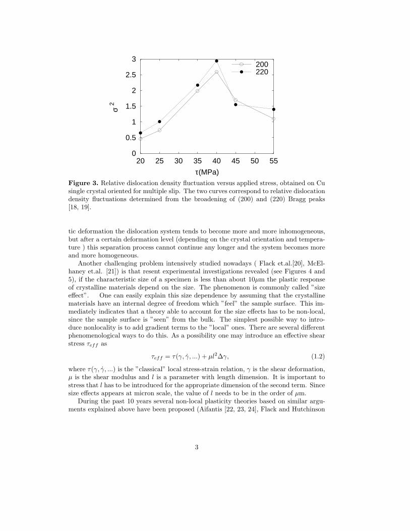
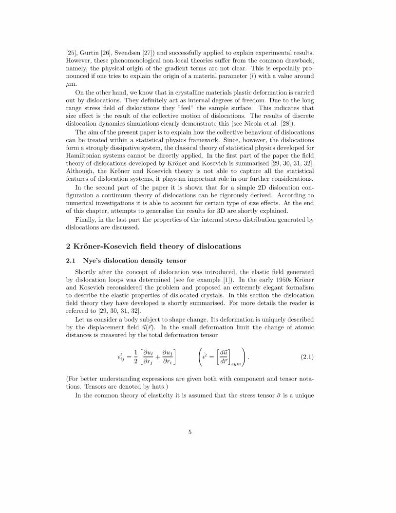
On the other hand TEM investigations revealed that dislocations formed during plas-tic deformation tend to form different dislocation patterns, like the cell structure (seeFigure 1.) developing at unidirectional load [4], or the so called ladder structure (see Fig-ure 2.) developing under cyclic loading [5]. In spite of several attempts (Kuhlmann-Wilsdorf et.al. [6, 7, 8], Holt [9], Walgraef and Aifantis[10, 11, 12], Kratochvil et.al.[13, 14, 15]) proposed to model the pattern formation, we are far from the completeunderstanding of this typically self organizing phenomena. One of the most strikingfeatures of the dislocation patterning, which is a great challenge to model, is the largevariety of the patterns observed. The variety manifests itself not just in the ”geometry”of the dense dislocation regions but also in several statistical properties of the differentdislocation ensembles. It is known for example that cyclic loading can lead to periodicstructures with well defined self selected length scale [5], while unidirectional loadingoften results in fractal like structures which do not have any length scales (Hahner et.al.[16, 17]). Another interesting feature of the patterning process observed recently by X-ray diffraction (Szekely et.al.[18, 19]) is that in case of unidirectional loading the relativedislocation density fluctuation σ2 defined as

σ2 = V

∫

ρ2(~r)d3r[∫

ρ(~r)d3r]2 , (1.1)

where ρ(~r) is the dislocation density and V is the crystal volumes, undergoes a sharpmaximum as deformation proceeds (see Figure 3). The result indicates that during plas-

1

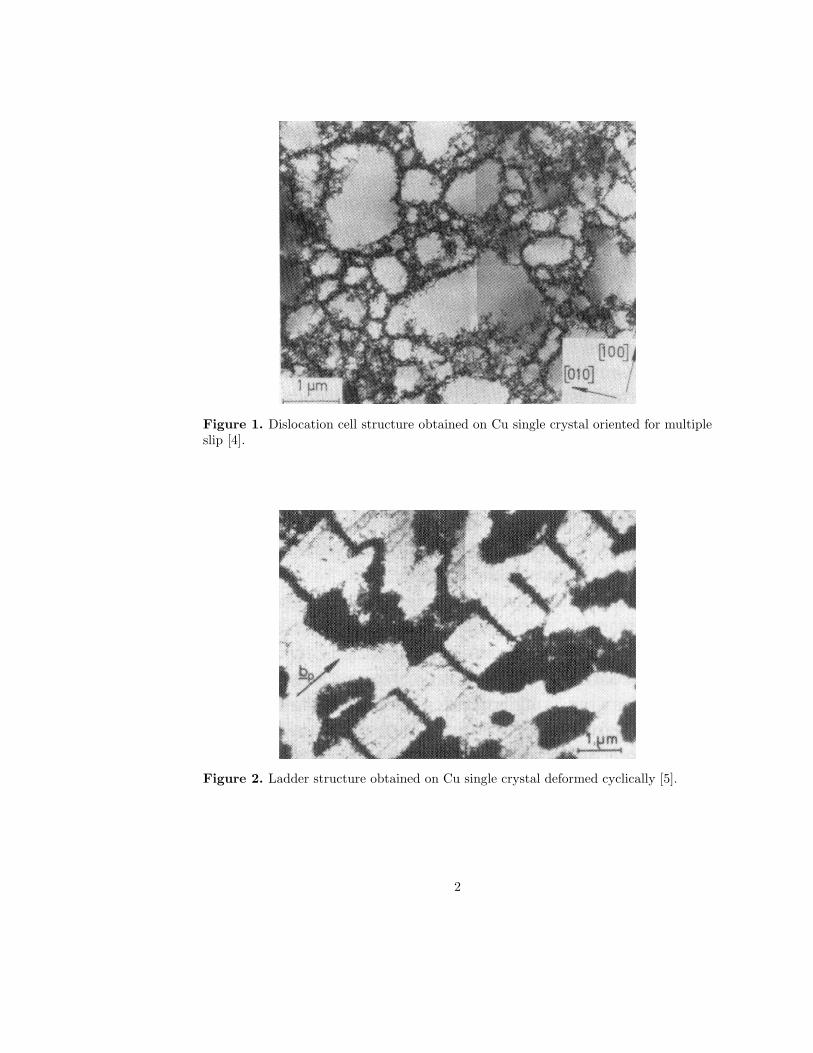
Figure 1. Dislocation cell structure obtained on Cu single crystal oriented for multipleslip [4].

Figure 2. Ladder structure obtained on Cu single crystal deformed cyclically [5].

2

0

0.5

1

1.5

2

2.5

3

20 25 30 35 40 45 50 55

σ 2

τ(MPa)

200220

Figure 3. Relative dislocation density fluctuation versus applied stress, obtained on Cusingle crystal oriented for multiple slip. The two curves correspond to relative dislocationdensity fluctuations determined from the broadening of (200) and (220) Bragg peaks[18, 19].

tic deformation the dislocation system tends to become more and more inhomogeneous,but after a certain deformation level (depending on the crystal orientation and tempera-ture ) this separation process cannot continue any longer and the system becomes moreand more homogeneous.

Another challenging problem intensively studied nowadays ( Flack et.al.[20], McEl-haney et.al. [21]) is that resent experimental investigations revealed (see Figures 4 and5), if the characteristic size of a specimen is less than about 10µm the plastic responseof crystalline materials depend on the size. The phenomenon is commonly called ”sizeeffect”. One can easily explain this size dependence by assuming that the crystallinematerials have an internal degree of freedom which ”feel” the sample surface. This im-mediately indicates that a theory able to account for the size effects has to be non-local,since the sample surface is ”seen” from the bulk. The simplest possible way to intro-duce nonlocality is to add gradient terms to the ”local” ones. There are several differentphenomenological ways to do this. As a possibility one may introduce an effective shearstress τeff as

τeff = τ(γ, γ, ...) + µl2∆γ, (1.2)

where τ(γ, γ, ...) is the ”classical” local stress-strain relation, γ is the shear deformation,µ is the shear modulus and l is a parameter with length dimension. It is important tostress that l has to be introduced for the appropriate dimension of the second term. Sincesize effects appears at micron scale, the value of l needs to be in the order of µm.

During the past 10 years several non-local plasticity theories based on similar argu-ments explained above have been proposed (Aifantis [22, 23, 24], Flack and Hutchinson

3

Figure 4. Normalised torque versus shear deformation obtained on torsionally deformedwires with different diameters a. The curves indicates, if a is smaller than 50µm, thehardening of the wires increase with decreasing diameter [20].

Figure 5. Microhardness versus indentation depth obtained on cold rolled Cu. It canbe seen, if the indentation depth is less than 1µm the microhardness increases withdecreasing indentation depth [21].

4

[25], Gurtin [26], Svendsen [27]) and successfully applied to explain experimental results.However, these phenomenological non-local theories suffer from the common drawback,namely, the physical origin of the gradient terms are not clear. This is especially pro-nounced if one tries to explain the origin of a material parameter (l) with a value aroundµm.

On the other hand, we know that in crystalline materials plastic deformation is carriedout by dislocations. They definitely act as internal degrees of freedom. Due to the longrange stress field of dislocations they ”feel” the sample surface. This indicates thatsize effect is the result of the collective motion of dislocations. The results of discretedislocation dynamics simulations clearly demonstrate this (see Nicola et.al. [28]).

The aim of the present paper is to explain how the collective behaviour of dislocationscan be treated within a statistical physics framework. Since, however, the dislocationsform a strongly dissipative system, the classical theory of statistical physics developed forHamiltonian systems cannot be directly applied. In the first part of the paper the fieldtheory of dislocations developed by Kroner and Kosevich is summarised [29, 30, 31, 32].Although, the Kroner and Kosevich theory is not able to capture all the statisticalfeatures of dislocation systems, it plays an important role in our further considerations.

In the second part of the paper it is shown that for a simple 2D dislocation con-figuration a continuum theory of dislocations can be rigorously derived. According tonumerical investigations it is able to account for certain type of size effects. At the endof this chapter, attempts to generalise the results for 3D are shortly explained.

Finally, in the last part the properties of the internal stress distribution generated bydislocations are discussed.

2 Kroner-Kosevich field theory of dislocations

2.1 Nye’s dislocation density tensor

Shortly after the concept of dislocation was introduced, the elastic field generatedby dislocation loops was determined (see for example [1]). In the early 1950s Kronerand Kosevich reconsidered the problem and proposed an extremely elegant formalismto describe the elastic properties of dislocated crystals. In this section the dislocationfield theory they have developed is shortly summarised. For more details the reader isrefereed to [29, 30, 31, 32].

Let us consider a body subject to shape change. Its deformation is uniquely describedby the displacement field ~u(~r). In the small deformation limit the change of atomicdistances is measured by the total deformation tensor

ǫtij =

1

2

[

∂ui

∂rj+

∂uj

∂ri

]

(

ǫt =

[

d~u

d~r

]

sym

)

. (2.1)

(For better understanding expressions are given both with component and tensor nota-tions. Tensors are denoted by hats.)

In the common theory of elasticity it is assumed that the stress tensor σ is a unique

5

function of the deformation tensor ǫt. In linear elasticity considered in this paper

σij = Lijklǫtlk

(

σ = L : ǫt)

(2.2)

where L is the tensor of elastic moduli.Deformation of a body, however, does not necessarily leads to the development of

internal stress. If we cut a body into two pieces along a plane, slide the two parts withrespect to each other and glue them together, the deformation is obviously nonzero alongthe plane, but the final stage is stress free. This means, the deformation can have a partwhich generates stress and another one which does not. According to this, the startingpoint of the plasticity theory explained below is that the gradient of the displacementfield commonly referred as total distortion is the sum of two terms, the so called plastic(βp) and elastic (β) distortion i.e.

∂uj

∂ri= βij + βp

ij

(

d~u

d~r= β + βp

)

. (2.3)

It needs to be mentioned, that the above expression is valid only in small deformationlimit. For large deformations, as a constitutive rule, it is commonly assumed that thefinal deformation stage of the body is reached by two successive steps, a plastic and anelastic deformation. For small deformations this is equivalent with Eq. (2.3 ). For thesake of simplicity we consider only this case.

Splitting the total distortion into two terms is rather formal so far. The plastic andelastic distortions need to be defined. It has to be mentioned at this point that, as it isexplained in details below, the separation is not unique.

As it is indicated by its name the elastic distortion is that part of the total one, whichis related to the stress developed in the body due to the deformation. In linear elasticity

σij = Lijklβlk

(

σ = L : β)

. (2.4)

However, due to the symmetric properties of L, σ determines only the symmetric partof β. With other words, the stress determines only the elastic deformation ǫ defined as

ǫij =1

2(βij + βji)

(

ǫ =[

β]

sym

)

. (2.5)

From Eqs. (2.4,2.5) the elastic deformation reads as

ǫij = L−1ijklσlk

(

ǫ = L−1 : σ)

, . (2.6)

where L−1 denotes the inverse of the tensor of elastic moduli.The next step is to define the plastic distortion. Since, by definition, the total distor-

tion is the gradient of the displacement field, it is curl free, i.e.

eikl∂

∂ri

∂uj

∂ri≡ 0

(

∇× d~u

d~r≡ 0

)

, (2.7)

6

where eikl is the antisymmetric tensor. The plastic distortion, however, is not necessarilycurl free. After Nye [33] the curl of the plastic distortion is called dislocation density

tensor α:

αij = eikl∂

∂rkβp

lj .(

α = ∇× βp)

(2.8)

(In the literature α is often refereed to Nye’s dislocation density tensor.) From Eqs.(2.3,2.7,2.8) one easily obtains that

αij = −eikl∂

∂rkβlj

(

α = −∇× β)

. (2.9)

In order to see the physical meaning of α introduced above, let us consider its integralfor an arbitrary surface A

bj =

∫

A

αijdAi. (2.10)

From the (2.9) expression of α, with the help of the Stockes’ theorem, one can find that

bj = −∫

A

eikl∂

∂rkβljdAi = −

∮

βijdsi = −∮

duei . (2.11)

Equation

bj = −∮

duei (2.12)

obtained is the one Burgers originally used [34] to define a dislocation as a singularityof the elastic displacement field ~ue. Therefore, α defined by Eq. (2.8) is the net Burgersvector of line singularities crossing a unit area. From Eq. (2.10) one can easily find thatfor a single straight dislocation

αij = libjδ(2)(ξ)

(

α = ~l ◦~b δ(2)(ξ))

, (2.13)

where ~l is the tangential vector of the dislocation line and ξ is the distance from the line.Before we proceed further, it should be mentioned that the dislocation density tensor

does not define uniquely the plastic distortion. Knowing α leaves βp uncertain up to agradient of an arbitrary vector field. However, as it is explained below, this does notaffect the stress field created by the dislocation system.

2.2 Internal stress generated by the dislocation system

In order to derive the field equations, let us consider the symmetric part of the totaldistortion. According to Eq. (2.3)

1

2

(

∂uj

∂ri+

∂ui

∂rj

)

= ǫij + ǫpij

(

[

d~u

d~r

]

sym

= ǫ + ǫp

)

, (2.14)

7

where ǫ and ǫp are the symmetric parts of the elastic and plastic distortions, respectively.Using the curl grad ≡ 0 identity one can find that

−eikmejln∂

∂rk

∂

∂rl

(

∂uj

∂ri+

∂ui

∂rj

)

≡ 0

(

∇×[

d~u

d~r

]

sym

×∇ ≡ 0

)

. (2.15)

It is useful to introduce the tensor operator inc (”incompatibility”) defined as

inc = −eikmejln∂

∂rk

∂

∂rl. (2.16)

With this definition Eq. (2.15) reads as

inc

[

d~u

d~r

]

sym

≡ 0. (2.17)

For further considerations it is useful to introduce the symmetric tensor field

ηij = −eikmejln∂

∂rk

∂

∂rlǫmn ( inc ǫ = η) . (2.18)

After a long but straightforward calculation one can obtain from Eqs. (2.8,2.14,2.17,2.18)that

ηij =1

2

(

ejln∂

∂rlαim + eiln

∂

∂rlαjm

)

(

η = [α ×∇]sym

)

. (2.19)

By substituting Eq. (2.6) into (2.18) we arrive at the equation that the stress createdby the dislocation has to fulfill:

ηij = −eikmejln∂

∂rk

∂

∂rlL−1

mnopσop

(

inc(

L−1σ)

= η)

. (2.20)

Since, for an arbitrary vector field ~f

inc

[

d~f

d~r

]

sym

≡ 0. (2.21)

Eq. (2.20) itself does not determine σ completely. However, supplementing it with theequilibrium condition

∂

∂riσij = 0 ( div σ = 0) (2.22)

we already have enough equations to determine the stress field generated by the disloca-tions.

8

2.3 Second order stress function tensor

Like in electrodynamics it is useful to reformulate Eqs. (2.20,2.22) into a potentialtheory. Let us introduce a second order stress function tensor χ defined with the relation

σij = −eikmejln∂

∂rk

∂

∂rlχmn (σ = inc χ) . (2.23)

Due to the identity

div inc ≡ 0 (2.24)

the (2.20) form of σ guarantees that the equilibrium condition (2.22) is fulfilled. Withthe stress function tensor introduced above Eq. (2.19) reads as

ηij = eikmejlneoqvepuwL−1mnop

∂

∂rk

∂

∂rl

∂

∂rq

∂

∂ruχvw

(η = inc(

L−1 inc χ))

. (2.25)

For an anisotropic medium the above equation is rather difficult to solve, but forisotropic materials, with shear modulus µ and Poisson’s ratio ν, a general solution canbe obtained. It is expedient to introduce another tensor potential χ′ defined as

χ′ij =

1

2µ

(

χij −ν

1 + 2νχkkδij

)

(2.26)

χij = 2µ

(

χ′ij +

ν

1 − νχ′

kkδij

)

. (2.27)

By inserting Eq. (2.27) into Eq. (2.25) one can find, if χ′ fulfills the gauge condition

∂

∂riχ′

ij = 0 ( div χ′ = 0) (2.28)

Eq. (2.23) simplifies to the biharmonic equation

∇4χ′ij = ηij

(

∇4χ′ = η)

. (2.29)

A remarkable feature of this equation is that the different components of χ′ obey separateequations making the problem much easier to solve. For an infinite medium the generalsolution of Eq. (2.29) is

χ′ij(~r) = − 1

8π

∫ ∫ ∫

|~r − ~r′|ηij(~r′)dV ′ (2.30)

2.4 2D problems

In the next section the statistical properties of an ensemble of parallel edge dislocationsare discussed. In this case the stress and the strain do not vary along the dislocation linedirection ~l. Taking ~l parallel to the z axis (with ~l = (0, 0,−1) in the above expressions the

9

derivatives with respect to z vanish (∂/∂z ≡ 0). One can find that Eq. (2.23) simplifiesto [30]:

σ11 = −∂2χ

∂y2, σ22 = −∂2χ

∂x2, σ12 =

∂2χ

∂x∂y, χ ≡ χ33 (2.31)

σ23 = −∂φ

∂x, σ13 =

∂φ

∂y, φ = −∂χ23

∂x+

∂χ31

∂y. (2.32)

Furthermore, from Eqs. (2.19,2.25) one obtains that the two scalar fields χ and φ intro-duced above obey the equations

∇4χ =2µ

1 − ν

(

b1∂

∂y− b2

∂

∂x

)

(ρd+ − ρd−) (2.33)

∇2φ = µb3(ρd+ − ρd−), (2.34)

where b1, b2 and b2 are the x, y, and z directional components of the Burgers vector,respectively. The notations ρd+ and ρd− stand for the dislocation densities with positiveand negative signs, respectively, They are the sum of δ(~r − ~ri) Dirac delta functions,were ~ri denotes the position of a dislocation. For the sake of simplicity we assumed thatall dislocations belong to the same slip system (single slip), but the expressions can beeasily generalised for multiple slip.

For an infinite medium the solutions of Eqs. (2.33,2.34) read as

χ(~r) =2µ

2π(1 − ν)

∫ (

b1∂

∂y′− b2

∂

∂x′

)

[ρd+(~r′) − ρd−(~r′)]R2 lnR d2~r′ (2.35)

and

φ(~r) = −µb3

2π

∫

[ρd+(~r′) − ρd−(~r′)] ln(R) d2~r′ (2.36)

where R = |~r − ~r′|.

2.5 Time evolution of the dislocation density tensor

As it is explained above, if we know the dislocation density tensor (i.e. we know thedislocation line geometry) the internal stress field can be determined from Eq. (2.25).This is however, only a ”static” description. In order to be able to describe the response ofthe dislocation system to external signals, the governing equations of the time evolutionof the dislocation density tensor should be determined.

If we take the partial time derivative (denoted by ” · ” ) of Eq. (2.8), we find that

αij + eikl∂

∂rkjlj = 0

(

˙α + ∇× j = 0)

(2.37)

10

where

j = − ˙βp (2.38)

is called dislocation current density [31]. The above equation is the ”conservation law ofthe Burgers vector” in differential form. Indeed, if we integrate both sides of Eq. (2.37)for an arbitrary area contoured by the closed curve L, according to Eq. (2.10), we obtainthat

dbj

dt= −

∮

L

jijdsi (2.39)

It is obvious from this relation that j is the Burgers vector carried by the dislocationscrossing a unit length part of the contour line L per unit time.

For an individual dislocation one can find that

jik = eilmllvmbkδ(2)(ξ)(

j = (~l × ~v) ◦~b δ(2)(ξ))

, (2.40)

where ~v is the velocity of the dislocation line at a given point. It is important to notethat if we added the gradient of an arbitrary vector field to j given above, this wouldalso satisfy the conservation law (2.37). The problem is obviously related to the non-uniqueness of the plastic distortion discussed earlier. However, expression (2.40) is theonly one which is physically meaningful. One expects that there is no plastic currentanywhere else but at the dislocation line. Nevertheless, strictly speaking we have topostulate this.

The above results clearly show that j has to be considered as an independent quantity.In order to be able to describe the time evolution of the dislocation system we have to setup a constitutive relation which gives how j depends on the dislocation density tensorand the external stress. Due to the long range nature of the dislocation-dislocation inter-action, the constitutive relation is obviously non-local in α. Beside this, the constitutiverelation has to be able to account for several different ”local” phenomena (self loop in-teraction, junction formation, annihilation etc.) making even more difficult to determineits form.

One possible approach to handle this problem is to set up the constitutive relationfrom phenomenological considerations. During the past years several phenomenologicalexpressions were proposed and successfully applied for modelling certain phenomena [26]but the problem is far not completely solved.

Another widely used approach to study the time evolution of dislocation systemsis discrete dislocation dynamics (DDD) simulation in which the dislocation loops areconsidered individually. After setting up velocity laws for the dislocation segments thedislocation loop geometry is updated numerically. Describing the actual numerical tech-niques used in DDD simulations is out of the scope of this paper. The reader can findthe details e.g. in [35, 36, 37, 38, 39, 40, 42, 43, 44, 45]. Although DDD simulations areextremely important for the better understanding of the collective properties of disloca-tions, due to their high computational demand their applicability in engineering practiceis limited.

11

2.6 Time evolution of the displacement field

In the previous part we have discussed how the stress field generated by the disloca-tions can be determined and what can be said in general about the time evolution of thedislocation density tensor. However, in many applications it is important to determinethe displacement field ~u(~r), too.

Let us go back to our starting equation (2.3), multiply it with the tensor of elasticmoduli L, and take the div of the equation. Using Eqs. (2.4,2.22) one obtains that

∂

∂riLijkl

∂uk

∂rl=

∂

∂riLijklβ

pkl

(

div Ld~u

d~r= div Lβp

)

. (2.41)

This is formally equivalent with the common equilibrium equation of elasticity with bodyforce density

fj = − ∂

∂riLijklβ

pkl

(

~f = − div Lβp)

(2.42)

Since, as it is explained earlier, the dislocation density tensor does not determine theplastic distortion uniquely, the above equation is not enough to determine the displace-ment field. Taking, however, the time derivative of Eq. (2.41), with the (2.38) definitionof j, one finds that

∂

∂riLijkl

∂uk

∂rl=

∂

∂riLijkljkl

(

div Ld~u

d~r= div Lj

)

. (2.43)

As it is discussed above, based on physical arguments, j can be uniquely defined, so thedeformation velocity field ~u can already be determined if j is known. Integrating it withrespect to time gives the change of the displacement field which is the quantity one canreally measure.

2.7 Problems related to coarse graining

The dislocation density tensor introduced above is a highly singular quantity. It isinfinite along the dislocation lines and vanishes elsewhere. More precisely, it is propor-tional to a delta function along the dislocation lines. The same holds for the dislocationcurrent density. The conservation law (2.37) guarantees that during the evolution of thedislocation system this delta function does not ”spread out”, only the shape of the loopscan change. This is certainly what we expect physically. This means, however, if wewant to follow the evolution of the system we have to follow the track of each dislocationloop as it is done in DDD simulations.

We may hope, like for many other physical systems, to predict the macroscopic re-sponse of the dislocation system, we do not need this detailed knowledge of the evolu-tion of the dislocation configuration. One should try to operate with locally averagedquantities. This means, the different quantities, like dislocation density tensor, stress,dislocation current density, etc., are convolved with a window function. In the physicsliterature the procedure is commonly called as ”coarse graining”, while in the engineering

12

community the term “homogenisation” is more frequently used. One can immediatelyraise the question what is the appropriate function we should use for the shape of thewindow function, and what determines its half width. One cannot have a general recipehow to resolve these problems. Nevertheless, we can hope that within certain limits theresult obtained by the coarse graining is not sensitive to the actual window functionshape and its width. If this is not the case, this clearly indicates that all the micro-scopical details are important. So, the coarse graining procedure always requires extracare. Beside this, it is important to stress that, before the equations obtained by coarsegraining are applied, for predicting the response of the material in a given situation, onealways has to study the relevance of the homogenisation.

In order to indicate the difficulties, as a simple example, let us consider a set of paralleledge dislocations with ±~b Burgers vectors parallel to the x axis. For this case Eq. (2.33)simplifies to

∇4χ =2µ

1 − ν

(

b∂

∂y

)

κd, (2.44)

where κd = ρd+ − ρd− is the signed dislocation density that is a sum of delta functions.If we take the convolution of Eq. (2.44) with a window function w(~r) we obtain that

∫

w(~r − ~r′)∇′4χ(~r′)d~r′ =2µ

1 − ν

∫

w(~r − ~r′)

(

b∂

∂y′

)

κd(~r)d~r′. (2.45)

After partial integrations we get that

∇4

∫

w(~r − ~r′)χ(~r′)d~r′ =2µ

1 − ν

(

b∂

∂y

)∫

w(~r − ~r′)κd(~r)d~r′. (2.46)

As it can be seen, the coarse grained fields denoted by

< χ >=

∫

w(~r − ~r′)χ(~r′)d~r′ < κ >=

∫

w(~r − ~r′)κd(~r′)d~r′ (2.47)

are related to each other as

∇4 < χ >=µ

1 − ν

(

b∂

∂y

)

< κ > (2.48)

that is formally equivalent with Eq. (2.44). With a similar argument, from Eq. (2.31)one can find that

< σ >11= −∂2 < χ >

∂y2, < σ >22= −∂2 < χ >

∂x2, < σ >12=

∂2 < χ >

∂x∂y. (2.49)

This means, the coarse grained fields are related to each other as the ”discrete” ones.However, important information is lost during coarse graining. If we consider two

dislocation configurations indicated in Figure 6 and coarse grain them for the samesquare areas indicated by the boxes, we get the same signed dislocation density value.On the other hand, it is obvious that the response of the two configurations are strongly

13

Figure 6. Two strongly different dislocation configurations giving the same κ if they arecoarse grained for the areas indicated by the boxes.

different, if one applies an external shear. So, in a continuum theory of dislocations,in which we operate with smooth fields, the coarse grained dislocation density tensoris not enough to characterise the state of the system. In the next section we discusshow a continuum theory can be derived from the equation of motion of straight paralleldislocations and what relevant quantities are needed to have an appropriate descriptionof this simple dislocation system on the mesoscopic scale.

3 Linking micro- to mesoscale for a 2D dislocation system

3.1 Discrete dislocation dynamics simulations in 2D

In the early 90s due to the fast increase of the available computer power it becamepossible to investigate the collective properties of dislocations by computer simulations.In DDD simulations the equations of motion of the dislocations (dislocation segments)are integrated numerically. During the past 15 years a vast amount of DDD simulationswere performed both in 2D [46, 47, 48, 49, 50, 51, 52, 53, 54, 55, 56] and 3D [35, 36, 37, 38,39, 40, 42, 43, 44, 45]. The detailed descriptions of the numerical methods applied andthe results obtained are out of the scope of the paper, but to demonstrate the potentialsand the limitations of the numerical simulations we will shortly review simulation resultsobtained by the author [50, 51] on the same system that is studied below in the statisticalphysics considerations.

In the simulations, the evolution of a system of parallel edge dislocations was studiedin a square area with periodic boundary conditions. (This means, the originally 3Dproblem was simplified to 2D.) The system was subject of unidirectional deformationwith a constant external deformation rate ǫ. The stress required to keep ǫ constant wascalculated. Dislocation motion was allowed in two slip systems (denoted by dotted linesin Figures 7) with 600 between the two slip directions. The system was oriented for singleslip, i.e. in one of the two slip systems the shear stress generated by the external loadwas much larger than in the other one.

In the simulations reported here only dislocation glide was allowed (i.e. the velocity ofthe dislocations were parallel to their Burgers vectors). In the equation of motion of the

14

dislocations, the inertia term (ma) was neglected beside the friction force ~Ff accountingfor the energy dissipation during dislocation motion. This is called overdamped dynamics.For simplicity, we assumed that ~Ff was proportional to the dislocation velocity, ~Ff =−B~v, where the coefficient B is called as dislocation mobility.

Beside the friction force, if the stress is nonzero at the dislocation, the Peach-Koehlerforce [1]

~FPK = ~l × (σ~b) (3.1)

also acts on a dislocation, where σ is the sum of the stress created by the dislocationsand the external stress. With these, the equation of motion of the ith dislocation is

~vi = B−1~si

~mi

N∑

j=1

σind(~rj − ~ri,~bj) + σext

~bi

(3.2)

where ~si and ~mi are unite vectors parallel and perpendicular to the slip direction of theith dislocation, respectively, σext is the external stress, and σind(~r − ~ri,~b) is the stress

field created by the ith dislocation (with Burgers vector~b). According to Eqs. (2.31,2.33),σind needs to be determined from the equations

∇4χind =2µ

1 − ν

(

b1∂

∂y− b2

∂

∂x

)

δ(~r − ~ri) (3.3)

σind11 = −∂2χind

∂y2, σind

22 = −∂2χind

∂x2, σind

12 =∂2χind

∂x∂y. (3.4)

For periodic boundary conditions used in the simulations σind does not depend on theabsolute position of the dislocation position. σind can be determined numerically eitherby the Fourier transformation of the above equation or by adding the σind

∞ stress of theappropriate periodic mirror dislocations, where σind

∞ is the stress in an infinite medium.It has to be mentioned here that for other boundary conditions Needleman and coworkersdeveloped an efficient method in which the stress is the sum of the stress the dislocationwould create in an infinite medium plus a ”compensating” component σcomp needed tofulfill the boundary conditions. Since σcomp is nonsingular at the dislocations it can becalculated with finite element methods.

During the system evolution dislocation multiplication was allowed with a global anda local conditions. The global condition was set up to reflect the experimental fact thata certain amount of external work is stored in the self-energy of dislocations. To mimicthis, if the external work increased a certain amount, a new dislocation dipole was added.Since the new dislocations are generated by the stress as a ”local” rule, the new dipolewas placed to a random position chosen with a probability proportional to the localstress. For the sake of simplicity dislocation annihilation was not taken into account.

A typical simulation result can be seen in Figure 7. As the stress-time relationobtained indicates, the system has a finite flow stress (the initial part of the curve islinear and reversible). This is the consequence of the relatively narrow random dipole

15

0 0.4 0.8 1.2-2.6

-2.4

-2.2

-2

-1.8

0 0.4 0.8 1.20

50

100

150

200

0 0.4 0.8 1.21

1.5

2

2.5

Elastic Energy

Dislocation Density

Applied Stress Stress

Time

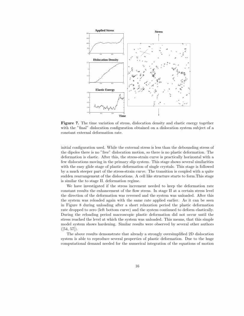
Figure 7. The time variation of stress, dislocation density and elastic energy togetherwith the ”final” dislocation configuration obtained on a dislocation system subject of aconstant external deformation rate.

initial configuration used. While the external stress is less than the debounding stress ofthe dipoles there is no ”free” dislocation motion, so there is no plastic deformation. Thedeformation is elastic. After this, the stress-strain curve is practically horizontal with afew dislocations moving in the primary slip system. This stage shows several similaritieswith the easy glide stage of plastic deformation of single crystals. This stage is followedby a much steeper part of the stress-strain curve. The transition is coupled with a quitesudden rearrangement of the dislocations. A cell like structure starts to form.This stageis similar the to stage II. deformation regime.

We have investigated if the stress increment needed to keep the deformation rateconstant results the enhancement of the flow stress. In stage II at a certain stress levelthe direction of the deformation was reversed and the system was unloaded. After thisthe system was reloaded again with the same rate applied earlier. As it can be seenin Figure 8 during unloading after a short relaxation period the plastic deformationrate dropped to zero (left bottom curve) and the system continued to deform elastically.During the reloading period macroscopic plastic deformation did not occur until thestress reached the level at which the system was unloaded. This means, that this simplemodel system shows hardening. Similar results were observed by several other authors([54, 57]).

The above results demonstrate that already a strongly oversimplified 2D dislocationsystem is able to reproduce several properties of plastic deformation. Due to the hugecomputational demand needed for the numerical integration of the equations of motion

16

Applied Stress

StrainPlastic & Applied def. rates

Time

Dislocations

Figure 8. Hardening obtained on the 2D dislocation system.

of the dislocations, one can afford only a couple of thousand dislocations in the sim-ulations. The problem is even more complex in 3D. At the moment about 1012m−2

dislocation density can be reached in a 10x10x10 µm box [45] applying the world largestsupercomputers. Although, these numerical investigations are extremely important, atthe moment their applicability is very limited in the engineering practice.

3.2 Continuum theories developed for other systems, analogies and differ-

ences

At the end of the 19th century Boltzmann developed the statistical theory of fluidsand gases. The key quantity he introduced is the density function f(t, ~r, ~p) giving theprobability density of finding an atom at the (~r, ~p) point of the phase space. From theconservation of the phase space volume (Liouville theorem) he obtained that the evolutionof f(t, ~r, ~p) is described by the relation

∂

∂tf(t, ~p, ~r) +

~p

m

∂

∂~rf(t, ~p, ~r) + ~F (~r)

∂

∂~pf(t, ~p, ~r) =

δfc

δt, (3.5)

where m is the mass of the atoms, ~F (~r) is the external force and δfc/δt is the so calledcollision term accounting for the momentum change occurring at the collision of twoatoms. Its actual form is difficult to determine. Since, however, the interaction betweenatoms is short ranged the collision is a local short event. This means that the collisiontime τc is much shorter than the mean collision free travelling time. As a consequenceof this the collision term can be well approximated with a relaxation term leading to theequation

∂

∂tf(t, ~p, ~r) +

~p

m

∂

∂~rf(t, ~p, ~r) + ~F (~r)

∂

∂~pf(t, ~p, ~r) = − 1

τc(f − f∞), (3.6)

17

where f∞ is the equilibrium Boltzmann distribution. An outstanding feature of Eq. (3.6)is that the Navier-Stokes equation of fluid dynamics can be derived from Eq. (3.6).

On the other hand it is obvious that Eq. (3.6) cannot be used for systems where theinteraction between the particles is long ranged. Plasma is a typical example for this.The Coulomb interaction between the charged particles is long ranged. The same holdsfor dislocations. The interaction between straight dislocations is proportional to 1/r.

For plasma, Vlasov obtained that the collision term δfc/δt is the sum of two terms

δfc

δt= −~Fsc(~r)

∂

∂~pf(t, ~p, ~r) + S(~r), (3.7)

where ~Fsc(~r) is the so called self-consistent field generated by the charge density ρc(~r)

and the electric current density ~jc(~r). The relations between ρc(~r), ~jc(~r), and ~Fsc(~r)determined by the Maxwell equations, are strongly non-local. However, due to the Debyescreening appearing in charged systems, the second term denoted by S(~r) is already local.According to these, for plasma the Boltzmann equation (3.5) reads as

∂

∂tf(t, ~p, ~r) +

~p

m

∂

∂~rf(t, ~p, ~r) +

[

~F (~r) + ~Fsc(~r)] ∂

∂~pf(t, ~p, ~r) = S(~r). (3.8)

As it is explained below, a similar equation can be derived for straight dislocations. Cer-tainly, the special properties of the dislocation-dislocation interaction and the dissipativenature of dislocation motion have to be taken into account.

3.3 Hierarchy of the different order density functions

Let us consider N straight parallel edge dislocations. As a first step let us assume thateach dislocation has the same Burgers vector~b parallel to the x axis. This simplification isneeded only to have shorter equations. The results obtained can be easily generalised. Inorder to get results that are physically relevant some generalisation is definitely needed.

For this case the equation of motion of the dislocations given by the general form(3.2) simplifies to

~vi = B−1~b

N∑

j 6=i

τind(~ri − ~rj) + τext

, (3.9)

where τext is the external shear and τind(~r) is the shear stress created by a dislocation.In an infinite isotropic medium

τind(~r) =bµ

2π(1 − ν)

x(x2 − y2)

(x2 + y2)2. (3.10)

As it is well known from statistical physics, instead of giving the time dependence ofthe coordinates of the N particles one can describe the state and the evolution of thesystem with the N particle probability density function fN varying in the 6N dimensionalphase space. Although, the dislocations form a nonconservative system, some of the re-sults of statistical mechanics can be applied. Since the equations of motion of dislocations

18

are only first order differential equations (assuming overdamped motion) for the problemconsidered, fN is a 2N dimensional function of the dislocation coordinates. By definitionfN (t, ~r1, ~r2...~rN )d2~r1d

2~r2, ..d2~rN is the probability of finding the N dislocations in the

d2~r1d2~r2..d

2~rN vicinity of the ~r1, ~r2...~rN points at time t.If we assume that the number of dislocations is conserved (later this restriction will

be lifted), fN has to fulfill the conservation law [58]

fN(t, ~r1, ~r2, ..., ~rN )d2~r1d2~r2, ..., d

2~rN =

fN(t + ∆t, ~r1 + ~v1∆t, ~r2 + ~v2∆t...~rN + ~vN∆t) (3.11)

×d2(~r1 + ~v1∆t)d2(~r2 + ~v2∆t)...d2(~rN + ~vN∆t).

The above relation reflects the simple fact that the probability of finding a dislocation ata certain point can change only if the dislocation moves from one point to another one.It is interesting to mention that in contrast with the conservative systems

fN (t, ~r1, ~r2, ..., ~rN ) 6=fN (t + ∆t, ~r1 + ~v1∆t, ~r2 + ~v2∆t, ..., ~rN + ~vN∆t), (3.12)

This is the consequence of that the d~r1d~r2...d~rN volume is not conserved during theevolution of the system.

After some simple algebraic manipulations Eq. (3.11) can be rewritten into a partialdifferentiation equation

∂fN

∂t+

N∑

i=1

∂

∂~ri{fN (t, ~r1, ~r2, ..., ~rN )~vi} = 0. (3.13)

By substituting the left hand side of Eq. (3.9) into ~vi we get that

∂fN

∂t+

N∑

i6=j

∂

∂~ri

{

fN~F (~ri − ~rj)

}

= 0 (3.14)

where ~F (~r) = ~bτind(~r). (B is dropped out from Eq. (3.14). With the appropriateselection of the time unit one can always take B = 1.) For the sake of simplicity in theabove equation the external shear was not taken into account. It is important to notethat Eq. (3.14) is mathematically equivalent with the original equations of motion of thedislocations (3.9). To find a solution of the two equations are equally difficult.

For many applications, however, we do not need that detailed description representedby the N particle probability density function. A less detailed description of the systemis the k-th order probability density function defined as

fk(~r1, ~r2, .., ~rk) =

∫ ∫

..

∫

fN(t, ~r1, ~r2...~rN )d2~rk+1d2~rk+2...d

2~rN . (3.15)

After integrating Eq. (3.14) with respect to the variables ~rk+1, ~rk+2, ..~rN , from the abovedefinition of fk (3.15) we obtain that

∂fk

∂t= −

N∑

i=1

N∑

j=1,j 6=i

∫

∂

∂~ri

{

fN~F (~ri − ~rj)

}

d2~rk+1d2~rk+2...d

2~rN . (3.16)

19

The double sum at the right hand side of the equation can be split into three parts

N∑

i=1

N∑

j=1,j 6=i

∫

∂

∂~ri

{

fN~F (~ri − ~rj)

}

d2~rk+1d2~rk+2...d

2~rN =

k∑

i=1

k∑

j=1,j 6=i

∂

∂~ri

{

fk~F (~ri − ~rj)

}

(3.17)

+k∑

i=1

N∑

j=k+1

∫

∂

∂~ri

{

fN~F (~ri − ~rj)

}

d2~rk+1d2~rk+2...d

2~rN

+

N∑

i=k+1

N∑

j=1,j 6=i

∫

∂

∂~ri

{

fN~F (~ri − ~rj)

}

d2~rk+1d2~rk+2...d

2~rN .

The last term is the integral of a div, so it can be transformed into a contour integralalong the border of the system. Assuming that the distribution functions tend to zerofast enough at infinity, this term vanishes. Taking into account that fN needs to beinvariant with respects to swapping the coordinates of two dislocations we get that

∂fk

∂t+

k∑

i=1

k∑

j=1,j 6=i

∂

∂~ri

{

fk~F (~ri − ~rj)

}

(3.18)

+(N − k)

∫

∂

∂~ri

{

fk+1~F (~ri − ~rk+1)

}

d2~rk+1 = 0.

As it can be seen the equation for the k-th order probability distribution functiondepends on the k+1-th order one. So, the reduction procedure applied results a hierarchyof the equations. In fluid dynamics and plasma physics this is called as BBGKY hierarchy.

For our further consideration the equations for f1 and f2 play an important role, sowe give their explicit forms [58]:

∂ρ1(~r1, t)

∂t+

∫

∂

∂~r1

{

ρ2(~r1, ~r2, t)~F (~r1 − ~r2)}

d2~r2 = 0 (3.19)

and

∂ρ2(~r1, ~r2, t)

∂t+

(

∂

∂~r1− ∂

∂~r2

)

ρ2(~r1, ~r2, t)~F (~r1 − ~r2)

+∂

∂~r1

∫

ρ3(~r1, ~r2, ~r3, t)~F (~r1 − ~r3)d2~r3 + 1 ↔ 2 = 0, (3.20)

where the notations ρ1 = Nf1, ρ2 = N(N−1)f2, ρ3 = N(N−1)(N−2)f3 were introduced.The advantage of using these quantities is that, in contrast with the probability densitiesf1, f2 and f3 normalised to 1, they are system size independent. They are commonlyreferred to as one, two and three particle density functions, respectively.

It is useful to show that Eq. (3.19) can be derived with another method, too [59].This can help to have a deeper understanding of the physical meaning of the equation

20

obtained. As a first step let us multiply (3.9) with δ(~r − ~ri) and take its derivative withrespect to ~r:

d

d~r

{

d~ri

dtδ(~r − ~ri)

}

=d

d~r

N∑

j 6=i

~F (~ri − ~rj)

δ(~r − ~ri)

. (3.21)

It is useful to introduce the ”discrete” dislocation density

ρd(~r) =

N∑

i=1

δ(~r − ~ri) (3.22)

that is the same as ρd+ defined in subsection 2.4, but since in the present analysis onlyone type of dislocation was considered, the subscript + was dropped. With this, the lefthand side of Eq. (3.21) can be rewritten into a weighted integral. Furthermore, takinginto account that

d

d~r

{

d~ri

dtδ(~r − ~ri)

}

= −d~ri

dt

d

d~riδ(~r − ~ri) = − d

dtδ(~r − ~ri), (3.23)

from Eq. (3.21) we get that

− d

dtδ(~r − ~ri) (3.24)

=d

d~r

{(∫

~F (~r − ~r′)[ρd(~r′) − δ(~r − ~r′)]d2~r′

)

δ(~r − ~ri)

}

(where δ(~r−~r′) beside ρd(~r′) is needed to avoid self dislocation interaction.) By summing

up with respect to i we conclude

− d

dtρd(~r) =

d

d~r

{(∫

~F (~r − ~r′)[ρd(~r′) − δ(~r − ~r′)]d2~r′

)

ρd(~r)

}

, (3.25)

which is a nonlinear strongly non-local equation for the ”discrete” dislocation densityρd(~r). Like it was done with the field equation (2.44), to get rid of the singular characterof ρd(~r) we can coarse grain Eq. (3.25). By introducing the coarse grained quantities

ρ1(~r) =< ρdisc(~r) > (3.26)

ρ2(~r1, ~r2) =< ρdisc(~r1)ρdisc(~r2) − ρdisc(~r1)δ(~r1 − ~r2 >, (3.27)

we get back Eq. (3.19) derived earlier. The procedure applied above clearly shows that theform of Eq. (3.19) does not depend on the actual form of the window function applied forthe coarse graining. However, ρ1(~r) and ρ2(~r1, ~r2) can depend on w(~r) chosen. Certainly,this is not a problem until we do not assume some relation between ρ1(~r) and ρ2(~r1, ~r2).We can say that Eq. (3.19) is exact but it is not enough to describe the time evolutionof the dislocation density.

21

Before we discuss how a closed theory can be obtained, the above results have tobe generalised for the case where Burgers vector of the dislocations are not the same.The simplest generalisation is if we allow that the Burgers vectors of the dislocationscan differ in sign. This is still a strong simplification of a real dislocation ensemble butan important step forward. Without going into the details with a similar procedureexplained above one can find that

∂ρ+(~r1, t)

∂t(3.28)

+~b∂

∂~r1

[

ρ+(~r1, t)τext +

∫

{ρ++(~r1, ~r2, t) − ρ+−(~r1, ~r2, t)} τind(~r1 − ~r2)d~r2

]

= 0

∂ρ−(~r1, t)

∂t(3.29)

+~b∂

∂~r1

[

−ρ−(~r1, t)τext +

∫

{ρ−−(~r1, ~r2, t) − ρ−+(~r1, ~r2, t)} τind(~r1 − ~r2)d~r2

]

= 0

where ~b is the Burgers vector of the positive signed dislocations. The subscripts ”+”and ”-” indicate the sign of the Burgers vector the different density functions are corre-sponding to. We mention here that the negative signs in front of ρ+− and ρ−+ in Eqs.(3.28) and (3.29) come from the simple fact that the interaction force acting betweendislocations with opposite signs is −Find.

By adding and substituting the two equations we obtain:

∂ρ(~r1, t)

∂t+~b

∂

∂~r1[κ(~r1, t)τext +

∫

{ρ++(~r1, ~r2, t) + ρ−−(~r1, ~r2, t)

−ρ+−(~r1, ~r2, t) − ρ−+(~r1, ~r2, t)}τind(~r1 − ~r2)d~r2] = 0, (3.30)

∂κ(~r1, t)

∂t+~b

∂

∂~r1[ρ(~r1, t)τext +

∫

{ρ++(~r1, ~r2, t) − ρ−−(~r1, ~r2, t)

−ρ+−(~r1, ~r2, t) + ρ−+(~r1, ~r2, t)}τind(~r1 − ~r2)d~r2] = 0 (3.31)

where ρ(~r, t) = ρ+(~r, t)+ρ−(~r, t) is the total and κ(~r, t) = ρ+(~r, t)−ρ−(~r, t) is the signeddislocation density. (κ is the same as < κ > introduced in Eq. (2.47) but to have shorterequations the brackets < .. > were omitted .)

3.4 Evolution of the plastic shear

Before we discuss how a closed theory can be obtained for the evolution of ρ and κ it isuseful to analyse the evolution of plastic shear. For the dislocation geometry consideredthe only non-vanishing component of the dislocation density tensor is

α31 = bκ. (3.32)

According to the definition of α given by Eq. (2.8) for the plane problem considered theonly component of the plastic distortion contributing to α31 is βp

21 and

bκ = −∂βp21

∂x. (3.33)

22

With the notation γ = βp21 commonly used, the above equation can be rewritten as

κ = −~b

b2

dγ

d~r, (3.34)

i.e. κ is proportional to the gradient of the plastic shear. With other words, this means,to get spatially varying plastic shear one has to introduce dislocations. This is why κ isoften called geometrically necessary dislocation (GND) density.

Taking the time derivative of Eq. (3.34) we get that

∂κ

∂t= −

~b

b2

dγ

d~r. (3.35)

By comparing this with Eq. (3.31) we obtain an explicit expression for the plastic shearrate γ:

γ = b2[ρ(~r1, t)τext (3.36)

+

∫

{ρ++(~r1, ~r2, t) − ρ−−(~r1, ~r2, t) − ρ+−(~r1, ~r2, t) + ρ−+(~r1, ~r2, t)}τind(~r1 − ~r2)d~r2].

3.5 Self-consistent field approximation

In order to have a closed continuum theory describing the evolution of the dislocationsystem, the (3.18) hierarchy of equations has to be cut at some order. In order to dothis, from some considerations independent from the Eq. (3.18) we have to give how thedensity functions with order higher than a given one can be built from the lower orderones. The simplest possible assumption is that the two particle density functions are theproducts of the one particle density functions [59], i.e.

ρss′(~r1, ~r2, t) = ρs(~r1)ρs′(~r2), s, s′ ∈ {+,−}. (3.37)

This means, that the short range correlations are neglected. As it is explained belowthis leads to a self-consistent field theory. Similar approximation is often used in plasmaphysics.

By substituting Eq. (3.37) into Eqs. (3.30,3.31) we arrive at

∂ρ(~r, t)

∂t+~b

∂

∂~r[κ(~r, t) {τsc(~r, t) + τext}] = 0, (3.38)

∂κ(~r, t)

∂t+~b

∂

∂~r[ρ(~r, t) {τsc(~r, t) + τext}] = 0, (3.39)

where

τsc(~r) =

∫

κ(~r1, t)τind(~r − ~r1)d~r1 (3.40)

23

is a field (with stress dimension) created by the coarse grained signed dislocation density.τsc is often called as self-consistent stress field. However, τsc is not a ”new” quantity.From Eq. (3.10) one can see that τsc fulfill the field equations

∆2χ =2bµ

(1 − ν)

∂

∂yκ(~r), τsc =

∂2

∂x∂yχ (3.41)

If we compare Eq. (3.41) with Eqs. (2.48, 2.49) we can see that τsc is nothing but thecoarse grained shear stress < σ >12.

It is important to note that dislocation multiplication and annihilation can also betaken into account by adding an f(ρ, τext + τsc, ...) source term to the right hand side ofEq. (3.38):

∂ρ(~r, t)

∂t+~b

∂

∂~r[κ(~r, t) {τsc(~r, t) + τext}] = f(ρ, τext + τsc, ...). (3.42)

Determining the actual form of the source term is a difficult issue. We will come backto this problem later on, but it has to be stressed at this point that Eq. (3.39) has toremain unchanged because it expresses that the total net Burgers vector of the dislocationsystem cannot change during deformation.

3.6 Stability analysis

Since dislocation multiplication is a ”local” event, it is plausible to assume that in agiven point the source term f(ρ, τext + τsc, ...) depends on only the local values of thedislocation density and the total shear stress τ = τext + τsc [59]. It is easy to see thatin this case Eqs. (3.39, 3.42) have a trivial solution that is κ(~r, t) = 0,and ρ(~r, t) = ρ0(t)where ρ0(t) is the solution of equation

dρ0

dt= f(ρ0, τext). (3.43)

Since, however, the equations are strongly nonlinear it is important to analyse thestability of this homogeneous solution [59]. For this, let us linearise Eqs. (3.38,3.39,3.41)around the trivial solution

d

dtρ′ +

∂

∂x{bτextκ

′} =∂f

∂ρ

∣

∣

∣

∣

ρ=ρ0

ρ′ +∂f

∂τ

∣

∣

∣

∣

τ=τext

τ ′, (3.44)

d

dtκ′ +

∂

∂x{b(τextρ

′ + ρ0τ′)} = 0, (3.45)

∆2χ′ =2bµ

(1 − ν)

∂

∂yκ′, τ ′ =

∂2

∂x∂yχ′, (3.46)

where κ′, ρ′ = ρ − ρ0, and τ ′ are small perturbations. The solution of the linearisedequations can be found in the form (assuming that ρ0(t) varies slowly in time)

τ ′(~r, t)κ′(~r, t)ρ′(~r, t)χ′(~r, t)

=

τ ′

κρ′

χ′

exp{λt + i(qxx + qyy)}. (3.47)

24

Substituting this form into the Eqs. (3.44-3.45) one can find that λ and the wave vector(qx, qy) have to fulfill the characteristic equation

∣

∣

∣

∣

∣

λ − ∂f∂ρ

∣

∣

∣

ρ=ρ0

iqxbτext + iT (Φ)qx

∂f∂τ

∣

∣

∣

τ=τext

iqxbτext λ + ρ0T (Φ)

∣

∣

∣

∣

∣

= 0, (3.48)

where

T (Φ) =2b2µ

(1 − ν)

q2xq2

y

(q2x + q2

y)2=

b2µ

2(1 − ν)sin2(2Φ), (3.49)

in which Φ is the angle between the x axis and the wave vector.The homogeneous solution is stable only if the real part of λ is non-positive for any

wave vector (qx, qy). This guarantees that there is no growing perturbation.As a first step let us analyse the stability of the homogeneous solution if the total

number of dislocations is conserved, i.e. if the source term f(ρ, τ) is zero. In this casethe solution of the characteristic equation (3.48) reads as

λ1,2 =−T (Φ)ρ0 ±

√

T (Φ)2ρ20 − 4(bτext)2q2

x

2. (3.50)

Since, T (Φ) is non-negative the real part of both λ1 and λ2 are non-positive, so inthe absence of source term the homogeneous solution is stable. However, an importantfeature of the linearised equations is that if the wave vector is parallel either to the xor the y axes the real parts of λ1 and λ2 vanish. This means, periodic perturbationswhich are either parallel or perpendicular to the Burgers vector neither growth nor dieout, they are marginally stable.

To see the influence of the source term f(ρ, τ) it is enough to study the sum of thetwo roots λ1 and λ2. From Eq. (3.48) we get that

λ1 + λ2 = −T (Φ)ρ0 +∂f

∂ρ

∣

∣

∣

∣

ρ=ρ0

. (3.51)

Since T (Φ) vanishes for Φ = 0 and Φ = 900, if ∂f/∂ρ is positive, there is a wave vectordomain where at least one of the two λ-s is positive. This means, if ∂f/∂ρ > 0 thehomogeneous solution is not stable any more.

3.7 Numerical studies

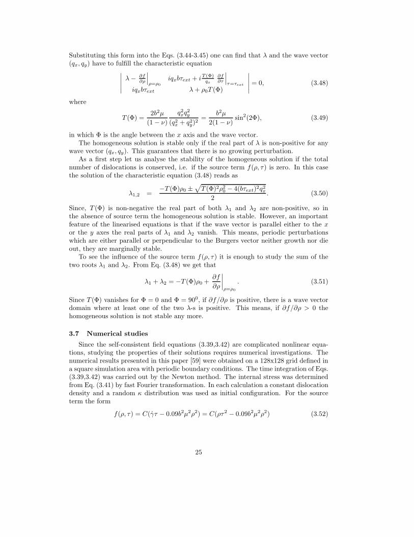
Since the self-consistent field equations (3.39,3.42) are complicated nonlinear equa-tions, studying the properties of their solutions requires numerical investigations. Thenumerical results presented in this paper [59] were obtained on a 128x128 grid defined ina square simulation area with periodic boundary conditions. The time integration of Eqs.(3.39,3.42) was carried out by the Newton method. The internal stress was determinedfrom Eq. (3.41) by fast Fourier transformation. In each calculation a constant dislocationdensity and a random κ distribution was used as initial configuration. For the sourceterm the form

f(ρ, τ) = C(γτ − 0.09b2µ2ρ2) = C(ρτ2 − 0.09b2µ2ρ2) (3.52)

25

was used. In expression (3.52) the first, dislocation creation term mimics the experi-mental observation that a certain amount of plastic work is stored as the self energy ofdislocations. The second, annihilation term simply expresses that annihilation requiresto have two dislocations close to each other. The constants are determined according tothe Taylor relation

τext = 0.3bµ√

ρ0, (3.53)

which we expect to hold at steady state.Since, apart from C, the size of the simulation area and the material parameters can

be scaled out from the equations the input parameters (ρ(t = 0, ~r), κ(t = 0, ~r), τext, C)and the results of the numerical calculations are given in arbitrary units.

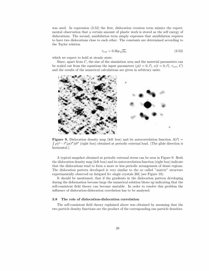
Figure 9. Dislocation density map (left box) and its autocorrelation function A(~r) =∫

ρ(~r − ~r′)ρ(~r′)d~r′ (right box) obtained at periodic external load. (The glide direction ishorizontal.)

A typical snapshot obtained at periodic external stress can be seen in Figure 9. Boththe dislocation density map (left box) and its autocorrelation function (right box) indicatethat the dislocations tend to form a more or less periodic arrangement of dense regions.The dislocation pattern developed is very similar to the so called ”matrix” structureexperimentally observed on fatigued fcc single crystals [60] (see Figure 10).

It should be mentioned, that if the gradients in the dislocation pattern developingduring the deformation become large the numerical solution blows up indicating that theself-consistent field theory can become unstable. In order to resolve this problem theinfluence of dislocation-dislocation correlation has to be analysed.

3.8 The role of dislocation-dislocation correlation

The self-consistent field theory explained above was obtained by assuming that thetwo particle density functions are the product of the corresponding one particle densities.

26

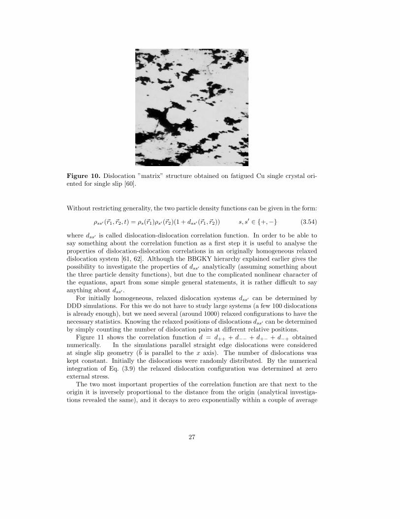
Figure 10. Dislocation ”matrix” structure obtained on fatigued Cu single crystal ori-ented for single slip [60].

Without restricting generality, the two particle density functions can be given in the form:

ρss′ (~r1, ~r2, t) = ρs(~r1)ρs′ (~r2)(1 + dss′ (~r1, ~r2)) s, s′ ∈ {+,−} (3.54)

where dss′ is called dislocation-dislocation correlation function. In order to be able tosay something about the correlation function as a first step it is useful to analyse theproperties of dislocation-dislocation correlations in an originally homogeneous relaxeddislocation system [61, 62]. Although the BBGKY hierarchy explained earlier gives thepossibility to investigate the properties of dss′ analytically (assuming something aboutthe three particle density functions), but due to the complicated nonlinear character ofthe equations, apart from some simple general statements, it is rather difficult to sayanything about dss′ .

For initially homogeneous, relaxed dislocation systems dss′ can be determined byDDD simulations. For this we do not have to study large systems (a few 100 dislocationsis already enough), but we need several (around 1000) relaxed configurations to have thenecessary statistics. Knowing the relaxed positions of dislocations dss′ can be determinedby simply counting the number of dislocation pairs at different relative positions.

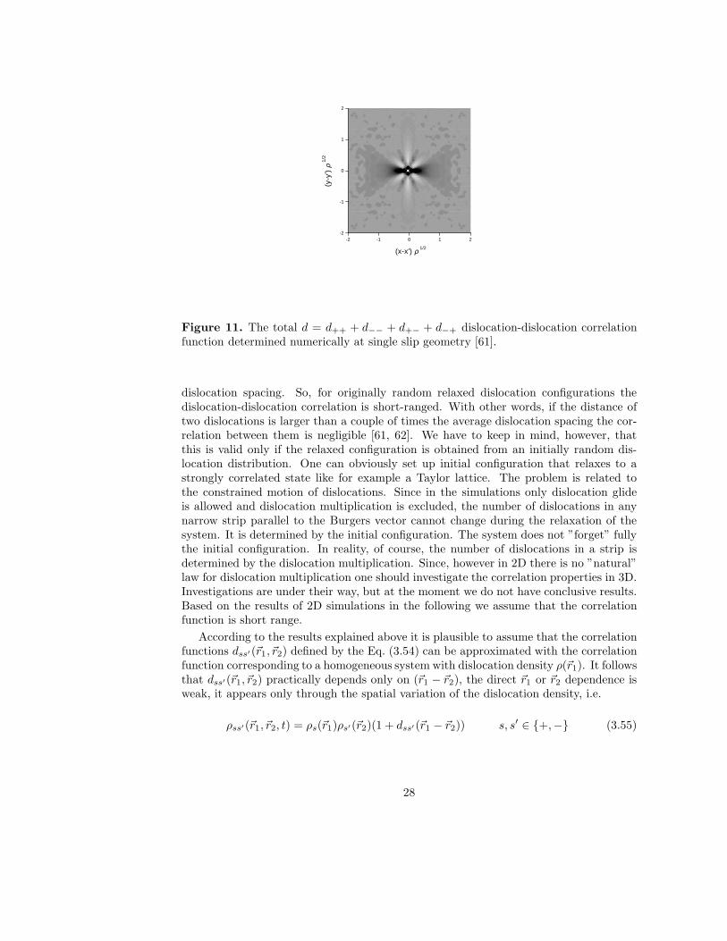
Figure 11 shows the correlation function d = d++ + d−− + d+− + d−+ obtainednumerically. In the simulations parallel straight edge dislocations were consideredat single slip geometry (~b is parallel to the x axis). The number of dislocations waskept constant. Initially the dislocations were randomly distributed. By the numericalintegration of Eq. (3.9) the relaxed dislocation configuration was determined at zeroexternal stress.

The two most important properties of the correlation function are that next to theorigin it is inversely proportional to the distance from the origin (analytical investiga-tions revealed the same), and it decays to zero exponentially within a couple of average

27

-2 -1 0 1 2-2

-1

0

1

2

(x-x') ρ 1/2

( y-y

') ρ 1

/2Figure 11. The total d = d++ + d−− + d+− + d−+ dislocation-dislocation correlationfunction determined numerically at single slip geometry [61].

dislocation spacing. So, for originally random relaxed dislocation configurations thedislocation-dislocation correlation is short-ranged. With other words, if the distance oftwo dislocations is larger than a couple of times the average dislocation spacing the cor-relation between them is negligible [61, 62]. We have to keep in mind, however, thatthis is valid only if the relaxed configuration is obtained from an initially random dis-location distribution. One can obviously set up initial configuration that relaxes to astrongly correlated state like for example a Taylor lattice. The problem is related tothe constrained motion of dislocations. Since in the simulations only dislocation glideis allowed and dislocation multiplication is excluded, the number of dislocations in anynarrow strip parallel to the Burgers vector cannot change during the relaxation of thesystem. It is determined by the initial configuration. The system does not ”forget” fullythe initial configuration. In reality, of course, the number of dislocations in a strip isdetermined by the dislocation multiplication. Since, however in 2D there is no ”natural”law for dislocation multiplication one should investigate the correlation properties in 3D.Investigations are under their way, but at the moment we do not have conclusive results.Based on the results of 2D simulations in the following we assume that the correlationfunction is short range.

According to the results explained above it is plausible to assume that the correlationfunctions dss′ (~r1, ~r2) defined by the Eq. (3.54) can be approximated with the correlationfunction corresponding to a homogeneous system with dislocation density ρ(~r1). It followsthat dss′(~r1, ~r2) practically depends only on (~r1 − ~r2), the direct ~r1 or ~r2 dependence isweak, it appears only through the spatial variation of the dislocation density, i.e.

ρss′(~r1, ~r2, t) = ρs(~r1)ρs′(~r2)(1 + dss′ (~r1 − ~r2)) s, s′ ∈ {+,−} (3.55)

28

Similar approximation is used successfully for many other systems like for example infirst principle quantum mechanics calculations to estimate the exchange energy. It iscalled ”local density approximation”.

By substituting Eq. (3.55) into Eqs. (3.30,3.31) after a long, but straightforwardcalculation we arrive at

∂ρ(~r, t)

∂t+~b

∂

∂~r[κ(~r, t) {τsc(~r) + τext − τf (~r) + τb(~r)}] = 0, (3.56)

∂κ(~r, t)

∂t+~b

∂

∂~r[ρ(~r, t) {τsc(~r) + τext − τf (~r) + τb(~r)}] = 0, (3.57)

where

τf (~r) =1

2

∫

ρ(~r1)da(~r − ~r1)τind(~r − ~r1)d~r1 (3.58)

τb(~r) =

∫

κ(~r1)d(~r − ~r1)τind(~r − ~r1)d~r1, (3.59)

in which the notations

d(~r) = 1/4[d++(~r) + d−−(~r) + d+−(~r) + d−+(~r)] (3.60)

da(~r) = 1/2[d+−(~r) − d−+(~r)] (3.61)

are introduced. Due to the following obvious symmetry properties of the correlationfunctions

d+−(~r) = d−+(−~r), d++(~r) = d++(−~r), d−−(~r) = d−−(−~r) (3.62)

d(~r) is an even, while da(~r) is an odd function of ~r. Furthermore, since the correlationfunctions correspond to a homogeneous system there is no other internal length scale butthe average dislocation spacing 1/

√ρ. It is obvious from simple dimensional analysis that

the correlation functions depend only on the dimensionless quantity ~r√

ρ, i.e. d(√

ρ~r)and da(

√ρ~r).

Taking into account that the corelation functions decay to zero within a few disloca-tion spacing the fields κ(~r1) and ρ(~r1) appearing in Eqs. (3.58,3.59) can be approximatedby their Taylor expansion around the point ~r. Keeping only the first nonvanishing termswe get that [61, 62]

τf (~r) =ρ(~r)

2

∫

da(~r)τind(~r)d~r, (3.63)

τb(~r) = −∂κ(~r)

∂~r

∫

~rd(~r)τind(~r)d~r. (3.64)

(To obtain expressions (3.63,3.64) one has to take into account the symmetry propertiesof d(~r) and da(~r) explained above, and the relation τind(~r) = −τind(−~r).)

29

With the variable substitution ~η =√

ρ~r, τf (~r) reads as

τf (~r) =

√

ρ(~r)

2

∫

da(~η)τind(~η)d2~η. (3.65)

where we took into account that τind is proportional to 1/|~r|. By substituting the actualform of τind given by Eq. (3.10) into Eq. (3.65) we get that

τf (~r) =AC

2b√

ρ(~r), (3.66)

where A = µ/[2π(1 − ν)] and

C =

∫

ηx(η2x − η2

y)

(η2x + η2

y)2d′a(ηx, ηy)dηxdηy. (3.67)

in which the prime in d′a(ηx, ηy) indicates that ~η has to be measured in unit of averagedislocation spacing. In order to see the physical meaning of the above expression, the ex-ternal stress dependence of the parameter C has to be analysed. The correlation functiond+− obviously varies with external stress (the equilibrium configuration of dislocationdipoles varies if stress is applied). Let us assume that the change of d+− resulted bythe external stress increases C. Since the change in d−+ is the opposite of the change ofd+− this causes also the increase of C because of the minus sign in front of d−+ in thedefinition of da. As we see, the parameter C depends on the external stress. Beside this,τf scales with

√ρ. These support association of τf with the flow stress. Certainly, we

have to be careful with this statement. In real dislocation systems hardening is caused bythe forest dislocations which are not included into our model in any sense. Nevertheless,a stress like term showing similar properties as the flow stress appears naturally in thetheory. The actual form of the stress dependence of C is difficult to determine, but onecan speculate that τf acts as static friction. It prevents dislocation motion, but it has amaximum scaling with

√ρ.

After this let us analyse τb in more details. With the same variable substitutionapplied above we get that

τb(~r) = −∂κ(~r)

∂~r

1

ρ(~r)

∫

~ηd′(~η)τind(~η)d2~τ. (3.68)

i.e.

τb(~r) = −AD~b

ρ

∂κ(~r)

∂~r, (3.69)

where

D =

∫

η2x(η2

x − η2y)

(η2x + η2

y)2d′(ηx, ηy)dηxdηy (3.70)

is a dimensionless constant. In contrast with C, D has only a weak external stressdependence because d(~r) contains the sum of the two correlation functions d+− and

30

d−+ changing oppositely. The actual value of D can only be determined numerically.According to the numerical studies explained below it is in the order of magnitude of 1.

With the results obtained above the evolution equations (3.56,3.57) read as

∂ρ(~r, t)

∂t+~b

∂

∂~r

[

κ(~r, t)

{

τ(~r, t) − τf − AD~b

ρ(~r, t)

∂κ(~r, t)

∂~r)

}]

= f(ρ, τ), (3.71)

∂κ(~r, t)

∂t+~b

∂

∂~r

[

ρ(~r, t)

{

τ(~r, t) − τf − AD~b

ρ(~r, t)

∂κ(~r, t)

∂~r

}]

= 0. (3.72)

where τ = τsc + τext is the total macroscopic stress.From Eq. (3.36) the constitutive equation of the plastic shear rate can also be given

as

γ = b2ρ(~r, t)

{

τ(~r, t) − τf − AD~b

ρ(~r, t)

∂κ(~r, t)

∂~r

}

. (3.73)

With Eq. (3.34)

γ = b2ρ(~r, t)

{

τ(~r, t) − τf − AD1

b2ρ(~r, t)

(

~b∂

∂~r

)2

γ(~r, t)

}

. (3.74)

If we introduce the effective stress

τeff (~r) = τ(~r) − AD1

b2ρ(~r)

(

~b∂

∂~r

)2

γ(~r) (3.75)

it looks similar to the effective stress (1.2) suggested by E. Aifantis from phenomenologicalconsiderations. An important difference, however, is that in Eq. (3.75) the length scalel = 1/

√ρ appearing in front of the gradient term is a natural one, it is not a material

parameter suggested in the phenomenological non-local continuum theories. The lengthscale 1/

√ρ obeys an evolution equation (Eq. (refrhof).

3.9 Deformation of a constrained channel

To illustrate some implications of the evolution equations derived in the previoussubsection we study a very simple example, namely a constrained channel deforming insimple shear as shown in Figure 12 [62]. A channel of width L in the x direction andinfinite extension in the y direction is bounded by walls that are impenetrable for dislo-cations (i.e., the plastic deformation in the walls is zero). The slip direction correspondsto the x direction, and the layer is sheared by a constant shear stress τext. The wholeassembly is embedded in an infinite crystal.

The system envisaged is particularly simple because it is homogeneous in the y di-rection (the dislocation densities depend on the coordinate x in the slip direction only).It follows from Eq. (3.41) that in this case the long-range self-consistent stress field iszero for an arbitrary function κ(x), i.e., any dislocation interactions in the system are of

31

y

x

LFigure 12. Geometry of a constrained channel

short-range nature and hence described by the flow stress τf and the gradient-dependentstress τb.

Before investigating the behaviour resulting from Eqs. (3.71) and (3.72) and compar-ing it with the results obtained from discrete simulations, it is instructive to have a lookat the results we get from the mean-field model defined by Eqs. (3.38) and (3.39). Sincethe self-consistent stress is zero, the mean-field model becomes trivial: Whatever theinitial conditions, for an arbitrarily small, positive value of the external stress all positivedislocations ’condense’ at the right wall and all negative dislocations at the left one. Foran initially homogeneous dislocation distribution with density ρ0, the strain achieved bythis condensation is γ∞ = ρ0bL/2. Hence, the system exhibits a trivial size effect (theachievable strain is proportional to the size of the system, which determines the meandislocation path). However, as demonstrated in the following, the prediction that thisstrain is achieved at arbitrarily small external stress is grossly unrealistic.

We now revert to the gradient-dependent model derived in the previous subsection.We assume an initially homogeneous dislocation distribution of density ρ0. To facilitatecomparison with discrete simulations, it is convenient to introduce scaled stress, spaceand dislocation density variables through τ = Ab

√ρ0τ , x = Dx/

√ρ, ρ = ρ0ρ, and

κ = ρ0κ. In scaled variables and after corresponding re-scaling of time, Eqs. (3.71) and(3.72) read

∂tρ(x, t) = −∂x [κ(x, t) {τ − [1/ρ(x, t)]∂xκ(x, t)}] , (3.76)

∂tκ(x, t) = −∂x [ρ(x, t) {τ − [1/ρ(x, t)]∂xκ(x, t)}] . (3.77)

To formulate the boundary conditions at the walls located at x = ±L/2, we note thatno dislocations can enter the system through the walls. Hence, the density of positivedislocations (moving to the right) at the left wall and the density of negative dislocationsat the right wall are zero, i.e. κ(−L/2) = −ρ(−L/2), κ(L/2) = ρ(L/2). Furthermore,the dislocation fluxes at the walls must be zero, which requires that [ρτ − ∂xκ] = 0 atx = ±L/2.

The initial conditions are ρ(x, 0) = 1 and κ(x, 0) = 0 everywhere except directly atthe walls where we assume non-zero values of κ in a narrow boundary layer to satisfy theboundary conditions. We make the simplifying assumption that the effective stress can be

32

represented as the external stress diminished by the (spatially homogeneous) flow stressof an infinite system, and perform a ’deformation experiment’ as follows: we increasethe effective stress from zero in an adiabatically slow manner, i.e., after each small stressincrement the system is allowed to relax until it reaches a stationary configuration. Afterthis relaxation, the scaled strain is calculated as γ = −

∫

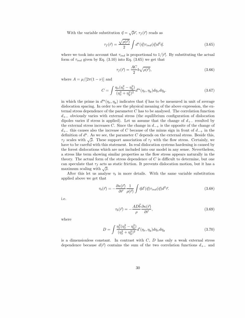
κdx (see Eq. (3.34)), then thestress is increased again, etc. The resulting stress-strain curves for different values of Lare compiled in Figure 13 [62]. It can be seen that the behaviour is very different from

0 2 4 6 8 100.0

0.5

1.0

1.5

2.0

2.5

Effe

ctiv

e st

ress

[ µbρ

01/2 /(

2 π(1

- ν))

]

Strain[bρ0

1/2D]

Figure 13. Stress-strain curves obtained at different channel size L.

-2 -1 0 1 2

-4

-2

0

2

4

-4

-2

0

2

4

γ [ D

bρ01/

2 ]

κ [ ρ

0]

x [ρ0

-1/2]

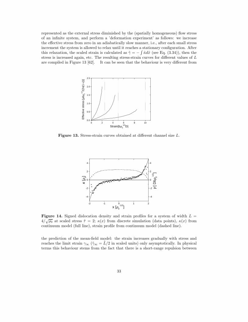
Figure 14. Signed dislocation density and strain profiles for a system of width L =4/

√ρ0 at scaled stress τ = 2; κ(x) from discrete simulation (data points), κ(x) from

continuum model (full line), strain profile from continuum model (dashed line).

the prediction of the mean-field model: the strain increases gradually with stress andreaches the limit strain γ∞ (γ∞ = L/2 in scaled units) only asymptotically. In physicalterms this behaviour stems from the fact that there is a short-range repulsion between

33

individual dislocations of the same sign as they pile up against the walls (see Figure 14).To increase the strain towards the asymptotic strain, this repulsion must be overcome,which requires an increasing stress that diverges as γ → γ∞.

Looking at the distribution of dislocation densities and strains within the channel,we find that at high stresses two boundary layers emerge near the walls (Figure 14). Itsproperties can be analysed by the equilibrium condition

τext − AD~b

ρ(~r, t)

∂κ(~r, t)

∂~r= 0 (3.78)

required to hold at steady state. (Since, for the geometry considered the self-consistentfield is zero, τ = τext). Near the boundaries most of the dislocations have the same sign,ρ ≈ |κ|. According to this, near the left boundary Eq. (3.78) reads as

τextκ = −ADbdκ(x)

dx(3.79)

with solution

κ(x) = κ0 exp{

− τext

ADbx}

. (3.80)

(A similar expression obviously holds near the right side, too.) As it is seen, the widthof the boundary layers decreases with increasing external stress.

It is interesting to compare this result with the prediction of the phenomenologicalgradient approach. According to Eq. (1.2) for the problem considered the equilibriumcondition is

τext −µ

l2κ(x)

dx= 0 (3.81)

with solution

κ(x) = κ0 +l2

µτextx (3.82)

In the centre part of the channel, where ρ is nearly constant, the linear relation predictedby the phenomenological gradient approach describes well the observed variation of κ,but it is not able to account for the boundary layers.

The results obtained are compared with DDD simulations performed on the samesystem. To get reliable statistics, stress-strain graphs and the corresponding dislocationdensity profiles were averaged over a huge ensemble (typically several thousands of sim-ulations). An example of a dislocation density profile obtained from this procedure isillustrated in Figure 14 which shows a κ(x) profile averaged over 2000 simulations ofsystems with length L = 4/

√ρ0 and (periodically repeated) height 16/

√ρ0. The profile

shown in the figure has been taken at a scaled effective stress τ = 2. It is seen thatindeed two boundary layers emerge. From the width of these boundary layers we candirectly determine the constant D for the present type of simulation, which turns outto be D = 0.8. Using the continuum model with this value of D yields the full line

34

02

46

81

00

.0

0.5

1.0

1.5

2.0

2.5

Effective stress [µbρ0

1/2/(2π(1-ν))]

Stra

in[b ρ

0 1/2D]

Figure 15. Comparison of stress-strain graphs; full line continuum model; data points:discrete simulation. Parameters are the same as in Figure 14.

in Figure 14, which shows that the density profile obtained from the continuum modelmatches well the discrete simulation except in the immediate vicinity of the walls.

As seen from Figure 15, also the stress-strain curves for the discrete and continuummodels exhibit almost perfect agreement. By varying the system size and initial dis-location density, we find that, for sufficiently high stresses the width of the boundarylayers at fixed stress τext is within the error margins indeed independent on the systemsize and the dislocation density. If the applied stress is increased, the boundary layerwidth is found to decrease. Again all these findings are in line with the predictions ofthe continuum model.

3.10 Application to metal-matrix composite

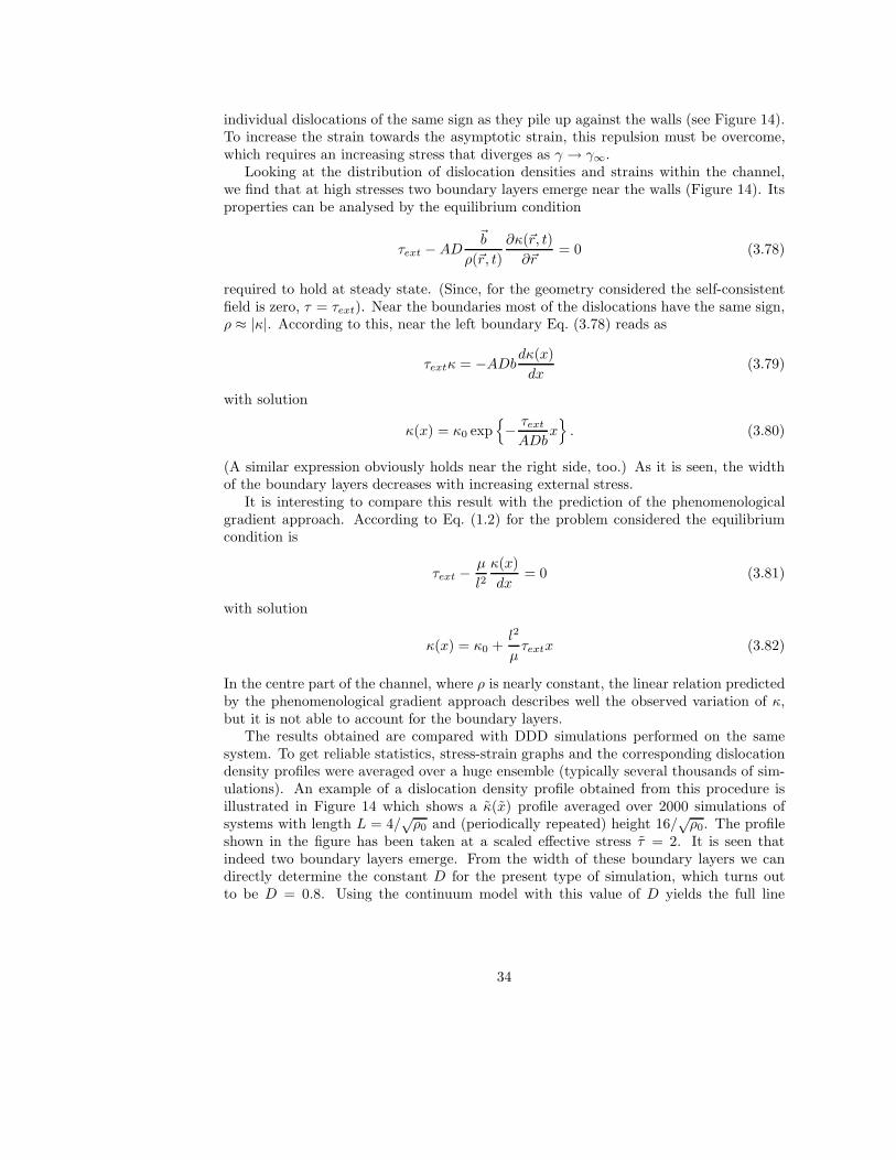
In order to demonstrate the capability of the continuum theory of dislocations ex-plained above we shortly summarise the simulation results obtained on a 2D modelsystem of a metal-matrix composite [54, 63]. It contains rigid rectangular particles ar-ranged in a hexagonal packing, as illustrated in Figure 16. The cell is subjected to planestrain, simple shear, which is prescribed through the boundary conditions

u1 = ±hΓ , u2 = 0 along x2 = ±h, (3.83)

35

2w 2 3h=

2h 2hf

2wf

U· hΓ·=

U· hΓ·=

x1

x2

Figure 16. Unit cell in a doubly-periodic array of elastic particles, subjected to simpleshear. The slip planes are taken to be parallel to the shear direction (x).

where Γ is the applied shear. Periodic boundary conditions are imposed along the lateralsides x = ±w. The slip plane normal ~n is in the y-direction and the Burgers vectoris parallel to the x-direction. Two reinforcement morphologies were analysed havingthe same area fraction of 20% but different geometric arrangements of the reinforcingphase. In one morphology, material (i), the particles are square and are separated byunreinforced veins of matrix material while in the other, material (iii), the particles arerectangular and do not leave any unreinforced veins of matrix material.

The problem was studied in details by Cleveringa et al. [54, 63] with DDD simulation.Here we compare their DDD simulation results with the results obtained by solving Eqs.(3.71,3.72) with a finite element method (for the details of the numerical technique usedsee [64, 65]). For the dislocation density field equations, boundary conditions need tobe specified at the boundary of the cell as well as along the interface with the elasticparticles. Along the cell sides x = ±w, periodic boundary conditions are applied, whilealong y = ±h we have the natural condition that there is no flux of dislocations acrossthese boundaries. Similar conditions apply along the top and bottom interfaces with theparticles. Along the vertical sides of the particles, we impose that the slip rate vanishes.

As it is seen in Figure 17 the stress-strain curves obtained by DDD simulation andfrom the continuum theory match extremely well for both reinforcement morphologiesinvestigated [64, 65]). Figure 18 shows the ρ and κ maps obtained for the (iii) morphol-ogy. It can be seen that, like at the shear of the channel discussed above, a boundarylayer of geometrically necessary dislocations develops at the vertical unpenetrable surfaceof the composite particles.

In conclusion it can be stated that for single slip the continuum theory developedpredicts the same behaviour as the DDD simulations. How to generalise the continuummodel to multiple slip is being studied intensively [66, 67]. At the moment the theory is

36

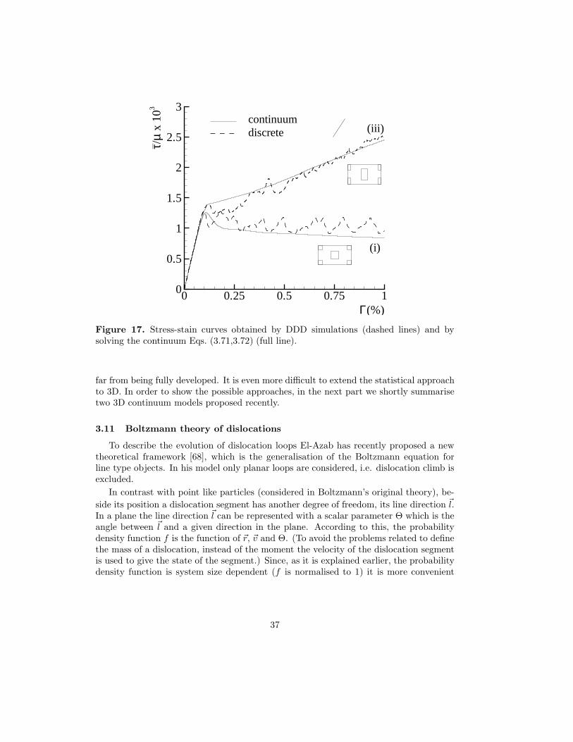
Γ(%)

τ/µ

x10

3

0 0.25 0.5 0.75 10

0.5

1

1.5

2

2.5

3

(i)

(iii)discretecontinuum

|

Figure 17. Stress-stain curves obtained by DDD simulations (dashed lines) and bysolving the continuum Eqs. (3.71,3.72) (full line).

far from being fully developed. It is even more difficult to extend the statistical approachto 3D. In order to show the possible approaches, in the next part we shortly summarisetwo 3D continuum models proposed recently.

3.11 Boltzmann theory of dislocations

To describe the evolution of dislocation loops El-Azab has recently proposed a newtheoretical framework [68], which is the generalisation of the Boltzmann equation forline type objects. In his model only planar loops are considered, i.e. dislocation climb isexcluded.

In contrast with point like particles (considered in Boltzmann’s original theory), be-

side its position a dislocation segment has another degree of freedom, its line direction ~l.In a plane the line direction ~l can be represented with a scalar parameter Θ which is theangle between ~l and a given direction in the plane. According to this, the probabilitydensity function f is the function of ~r, ~v and Θ. (To avoid the problems related to definethe mass of a dislocation, instead of the moment the velocity of the dislocation segmentis used to give the state of the segment.) Since, as it is explained earlier, the probabilitydensity function is system size dependent (f is normalised to 1) it is more convenient

37

-1 0 1-1

0

1400350300250200150100500

ρL2

-1 0 1-1

0

14003002001000

-100-200-300-400

κL2

Figure 18. ρ (top box) and κ (bottom box) maps at 1$ deformation for the (iii) mor-phology.

to operate with dislocation line length density φ. Hence, φ(i)(~r, ~v, Θ, t) can be given the

definition: φ(i)(~r, ~v, Θ, t)d3~rd3~vdΘ is the dislocation line length with Burgers vector ~bi

(i = 1..N) in the d3~rd3~vdΘ phase space at time t. It has to be noted that since ~v is

perpendicular to ~l, Θ is not an ”independent” variable, that is why it does not appearamong the arguments of φ(i).

The conventional field variables are now derived from φ(i). The dislocation line densityis defined as follows:

ρ(~r, t) =

N∑

i=1

ρ(i)(~r, t) (3.84)

where

ρ(i)(~r, t) =

∫ ∫

φ(i)(~r, ~v, Θ, t)d3~vdΘ (3.85)

38

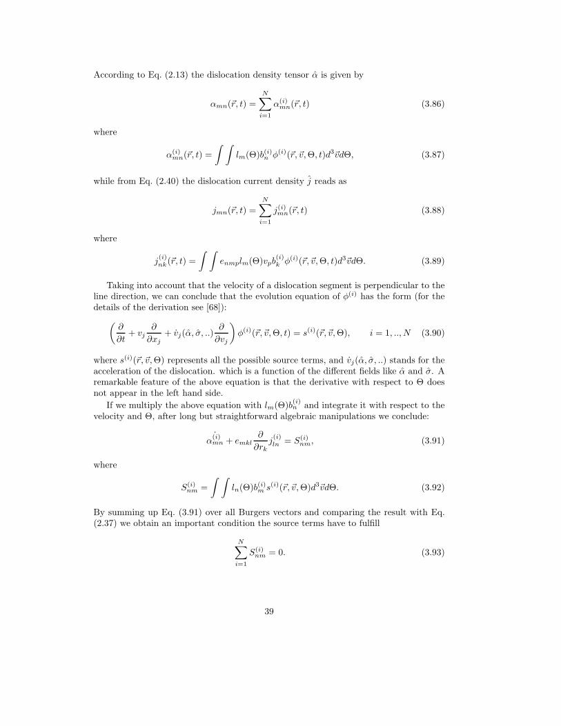
According to Eq. (2.13) the dislocation density tensor α is given by

αmn(~r, t) =N∑

i=1

α(i)mn(~r, t) (3.86)

where

α(i)mn(~r, t) =

∫ ∫

lm(Θ)b(i)n φ(i)(~r, ~v, Θ, t)d3~vdΘ, (3.87)

while from Eq. (2.40) the dislocation current density j reads as

jmn(~r, t) =

N∑

i=1

j(i)mn(~r, t) (3.88)

where

j(i)nk(~r, t) =

∫ ∫

enmplm(Θ)vpb(i)k φ(i)(~r, ~v, Θ, t)d3~vdΘ. (3.89)

Taking into account that the velocity of a dislocation segment is perpendicular to theline direction, we can conclude that the evolution equation of φ(i) has the form (for thedetails of the derivation see [68]):

(

∂

∂t+ vj

∂

∂xj+ vj(α, σ, ..)

∂

∂vj

)

φ(i)(~r, ~v, Θ, t) = s(i)(~r, ~v, Θ), i = 1, .., N (3.90)

where s(i)(~r, ~v, Θ) represents all the possible source terms, and vj(α, σ, ..) stands for theacceleration of the dislocation. which is a function of the different fields like α and σ. Aremarkable feature of the above equation is that the derivative with respect to Θ doesnot appear in the left hand side.

If we multiply the above equation with lm(Θ)b(i)n and integrate it with respect to the

velocity and Θ, after long but straightforward algebraic manipulations we conclude:

˙α

(i)mn + emkl

∂

∂rkj(i)ln = S(i)

nm, (3.91)

where

S(i)nm =

∫ ∫

ln(Θ)b(i)m s(i)(~r, ~v, Θ)d3~vdΘ. (3.92)

By summing up Eq. (3.91) over all Burgers vectors and comparing the result with Eq.(2.37) we obtain an important condition the source terms have to fulfill

N∑

i=1

S(i)nm = 0. (3.93)

39

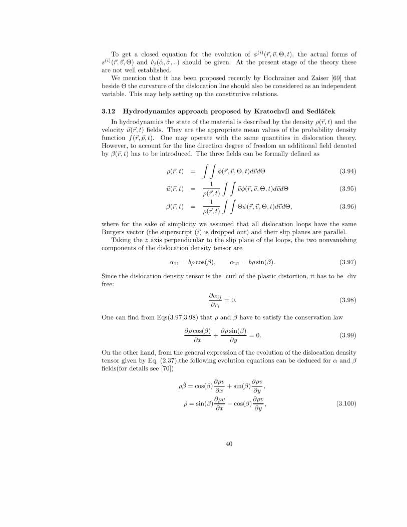
To get a closed equation for the evolution of φ(i)(~r, ~v, Θ, t), the actual forms ofs(i)(~r, ~v, Θ) and vj(α, σ, ..) should be given. At the present stage of the theory theseare not well established.

We mention that it has been proposed recently by Hochrainer and Zaiser [69] thatbeside Θ the curvature of the dislocation line should also be considered as an independentvariable. This may help setting up the constitutive relations.

3.12 Hydrodynamics approach proposed by Kratochvıl and Sedlacek

In hydrodynamics the state of the material is described by the density ρ(~r, t) and thevelocity ~u(~r, t) fields. They are the appropriate mean values of the probability densityfunction f(~r, ~p, t). One may operate with the same quantities in dislocation theory.However, to account for the line direction degree of freedom an additional field denotedby β(~r, t) has to be introduced. The three fields can be formally defined as

ρ(~r, t) =

∫ ∫

φ(~r, ~v, Θ, t)d~vdΘ (3.94)

~u(~r, t) =1

ρ(~r, t)

∫ ∫

~vφ(~r, ~v, Θ, t)d~vdΘ (3.95)

β(~r, t) =1

ρ(~r, t)

∫ ∫

Θφ(~r, ~v, Θ, t)d~vdΘ, (3.96)

where for the sake of simplicity we assumed that all dislocation loops have the sameBurgers vector (the superscript (i) is dropped out) and their slip planes are parallel.

Taking the z axis perpendicular to the slip plane of the loops, the two nonvanishingcomponents of the dislocation density tensor are

α11 = bρ cos(β), α21 = bρ sin(β). (3.97)

Since the dislocation density tensor is the curl of the plastic distortion, it has to be divfree:

∂αij

∂ri= 0. (3.98)

One can find from Eqs(3.97,3.98) that ρ and β have to satisfy the conservation law

∂ρ cos(β)

∂x+

∂ρ sin(β)

∂y= 0. (3.99)

On the other hand, from the general expression of the evolution of the dislocation densitytensor given by Eq. (2.37),the following evolution equations can be deduced for α and βfields(for details see [70])

ρβ = cos(β)∂ρv

∂x+ sin(β)

∂ρv

∂y,

ρ = sin(β)∂ρv

∂x− cos(β)

∂ρv

∂y, (3.100)

40

where v = |~v|.To have a closed theory a constitutive relation is needed between the three fields

ρ(~r, t), β(~r, t) and v(~r, t). Kratochvıl and Sedlacek [70] suggested the following constitu-tive relation for the velocity field :

Bv =

bσ13 + Cκs − bτ0 − bτ if bσ13 + Cκs > bτ0 + bτ0 if |bσ13 + Cκs| < bτ0 + bτbσ13 + Cκs + bτ0 + bτ if bσ13 + Cκs < −bτ0 − bτ

(3.101)

where bσ13 is the Peach-Koehler force due to the local shear stress, Cκs is the self-force,bτ0 is the friction force, and bτ represents the interaction between the gliding dislocationsan the dislocation loops.

The self-force Cκs is considered in the line tension approximation, where κs is thedislocation line tension. The curvature of a dislocation segment C(~r, β, t) = − div~n,where ~n is the unit normal to the dislocation segment. As it is explained in details in[70] C can be approximated by the expression

C = cos(β)∂β

∂x+ sin(β)

∂β

∂y(3.102)

The most difficult problem is to set up an appropriate expression for bτ . For this Kra-tochvıl and Sedlacek [70] suggested that

bτ = Fc1/3 (3.103)

were c is the loop density, and F is a constant.According to detailed analytical and numerical investigations [70] the model explained

above is able to predict both dislocation patterning and size effect. Nevertheless, thejustification of the assumptions used requires further investigation.

4 Internal stress distribution generated by the dislocations

In order to describe the statistical properties of a dislocation ensemble, a key quantityis the internal stress distribution. In this section the general form of the probabilitydistribution of the internal shear stress P (τ) is determined for a system of parallel edgedislocations. As it is discussed later the results can be generalised to 3D systems.

4.1 General considerations

Like in the previous section, let us consider a system of N parallel straight edgedislocations positioned at the points ~ri, i = 1, N in the xy plane perpendicular to thedislocation lines. For the sake of simplicity, we assume that each dislocation has thesame Burgers vector ~b. As it is shown later, the generalisation of the results for systemsconsisting of dislocations with different Burgers vectors is straightforward [71].

The internal shear stress at the point ~r is the sum of the stress fields of the individualdislocations

τ(~r) =

N∑

i=1

τind(~r − ~ri). (4.1)

41

In the first part of our analysis we assume that there is no dislocation at the point ~r.Later on, the stress distribution at the dislocations is discussed, too.

The precise definition of the problem addressed in this section is to determine theP (τ0)dτ0 probability of occurrence of τ in the range

τ0 −dτ0

2≤ τ(~r) ≤ τ0 +

dτ0

2(4.2)

where τ0 is a preassigned value for τ . P (τ0) can be obtained as a direct application ofMarkoff’s method [72] applied for several problems, like the problem of random flights, orfor the determination of the distribution of forces in gravitationally interacting randomsystems. In contrast with the two problem mentioned, for dislocations the N particledistribution function cannot be built up from the one particle distribution functionssince as it will be shown later it would lead to system size dependent internal stressdistribution function P (τ0). To avoid this, dislocation-dislocation correlation must betaken into account.

Denoting the N particle dislocation density function by fN(~r1, ~r2, . . . , ~rN ) the internalstress distribution can be expressed as

P (τ0)dτ0 =

∫

. . .

∫

fN (~r1, ~r2, . . . , ~rN )d~r1d~r2 . . . d~rN , (4.3)

where the integration is effected only over that part of configuration space for which theinequalities (4.2) are satisfied. By the introduction of the factor

∆(~r1, ~r2, . . . , ~rN ) =

{

1 whenever τ0 − dτ0

2 ≤ τ ≤ τ0 + dτ0

20 otherwise.

(4.4)

the integral in Eq. (4.3) can be extended over 2N dimensional space ℜ2N :

P (τ0)dτ0 =

∫ ∞

−∞

. . .

∫ ∞

−∞

∆(~r1, ~r2, . . . , ~rN )fN (~r1, ~r2, . . . , ~rN )d~r1d~r2 . . . d~rN . (4.5)

For the determination on the structure of expression (4.5) one has to consider the integral

δ =1

π

∫ ∞

−∞

sin(αq)

qexp[iγq]dq, (4.6)

which is the well-known discontinuous integral of the Dirichlet function with the proper-ties

δ =

{

1 whenever −α < γ < α0 otherwise.

(4.7)

By taking

α =dτ0

2and γ =

N∑

i=1

τind(~r − ~ri) − τ0 (4.8)

42

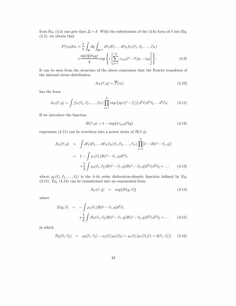
from Eq. (4.4) one gets that ∆ = δ. With the substitution of the (4.6) form of δ into Eq.(4.5), we obtain that

P (τ0)dτ0 =1

π

∫

ℜ

dq

∫

ℜ2N

d~r1d~r2 . . . d~rNfN(~r1, ~r2, . . . , ~rN )

× sin(12dτ0q)

qexp

{

i

[

N∑

i=1

τind(~r − ~ri)q − τ0q

]}

. (4.9)

It can be seen from the structure of the above expression that the Fourier transform ofthe internal stress distribution

AN (~r, q) = P (τ0) (4.10)

has the form

AN (~r, q) =

∫

fN (~r1, ~r2, . . . , ~rN )N∏

j=1

exp {iqτ(~r − ~rj)} d2~r1d2~r2 . . . d2~rN . (4.11)

If we introduce the function

B(~r, q) = 1 − exp{iτind(~r)q} (4.12)

expression (4.11) can be rewritten into a power series of B(~r, q)

AN (~r, q) =

∫

d~r1d~r2 . . . d~rNfN(~r1, ~r2, . . . , ~rN )N∏

j=1

[1 − B(~r − ~rj , q)]

= 1 −∫

ρ1(~r1)B(~r − ~r1, q)d2~r1

+1

2

∫

ρ2(~r1, ~r2)B(~r − ~r1, q)B(~r − ~r2, q)d2~r1d

2~r2 + . . . (4.13)

where ρk(~r1, ~r2, . . . , ~rk) is the k-th order dislocation-density function defined by Eq.(3.15). Eq. (4.13) can be transformed into an exponential form

AN (~r, q) = exp{E(q, ~r)} (4.14)

where

E(q, ~r) = −∫

ρ1(~r1)B(~r − ~r1, q)d2~r1

+1

2

∫

D2(~r1, ~r2)B(~r − ~r1, q)B(~r − ~r2, q)d2~r1d

2~r2 + . . . (4.15)

in which

D2(~r1, ~r2) = ρ2(~r1, ~r2) − ρ1(~r1)ρ1(~r2) = ρ1(~r1)ρ1(~r2)(1 + d(~r1, ~r2)) (4.16)

43

is the dislocation-dislocation correlation function.Eq. (4.15) is straightforward to generalise for the case where dislocations with Burgers

vectors ±~b are allowed. One can find that

E(q, ~r) = −∫

[ρ+(~r1)B(~r − ~r1, q) + ρ−(~r1)B∗(~r − ~r1, q)] d

2~r1

+1

2

∫

D++(~r1, ~r2)B(~r − ~r1, q)B(~r − ~r2, q)d2~r1d

2~r2

+1

2

∫

D+−(~r1, ~r2)B(~r − ~r1, q)B∗(~r − ~r2, q)d

2~r1d2~r2

+1

2

∫

D−−(~r1, ~r2)B∗(~r − ~r1, q)B

∗(~r − ~r2, q)d2~r1d

2~r2

+1

2

∫

D−+(~r1, ~r2)B∗(~r − ~r1, q)B(~r − ~r2, q)d

2~r1d2~r2 + . . . (4.17)

where ”*” denotes complex conjugate.

4.2 Stress distribution at the dislocations

In the previous subsection we assumed that there is no dislocation at point ~r at whichthe probability of the internal stress is determined. One can also ask the probabilitydistribution of the shear stress at the dislocations P c(τ).

Let assume that the dislocation at which we ask the probability distribution is at thepoint ~r1. The stress at the dislocation is obviously

τ(~r1) =

N∑

i=2

τind(~r1 − ~ri). (4.18)

The derivation procedure explained above can be repeated for this case, but fN(~r1, ~r2, . . . , ~rN )needs to be replaced with the conditional probability density f c(~r2, . . . , ~rN |~r1).f c(~r2, . . . , ~rN |~r1)d~r2d~r3..d~rN is the the probability of finding the 2nd, 3th, .. Nth dislo-cation in the d~r2d~r3..d~rN vicinity of points ~r2, ~r3..~rN assuming there is a dislocation atpoint ~r1. One gets that the Fourier transform of P c(τ) reads as

Ac(~r, q) =

∫

d2~r2d2~r3 . . . d2~rNf c(~r2, . . . , ~rN |~r1)

N∏

j=2

[1 − B(~r1 − ~rj , q)] (4.19)

The conditional probability f c(~r2, . . . , ~rN |~r1) can be given as

f c(~r2, . . . , ~rN |~r1) =fN(~r1, ~r2, . . . , ~rN )

f1(~r1). (4.20)

Substituting this into Eq. (4.19) and rewriting it into a power series of B(~r, q) we obtain

Ac(~r1, q) = 1 −∫ [

ρ++(~r1, ~r2)

ρ+(~r1)B(~r1 − ~r2, q)

+ρ+−(~r1, ~r2)

ρ+(~r1)B∗(~r1 − ~r2, q)

]

d2~r2 + ... (4.21)

44

where we assumed that the dislocation at point ~r1 has positive Burgers vector. (A similarexpression holds for dislocations with negative Burgers vector.)

4.3 The mean values of distributions P (τ) and P c(τ)

Since dislocations form strongly inhomogeneous distributions the explicit form ofP (τ) and P c(τ) cannot be determined analytically. Nevertheless, analytical results canbe obtained for some of their properties [71, 73].

An important characteristic value of a distribution function P (x) is its mean value< x >=

∫

xP (x)dx. As it is well known the mean value can be determined from theA(q) Fourier transform of the distribution function by the relation

< x > =i

A(0)

dA(q)

dq

∣

∣

∣

∣

q=0

(4.22)

Applying the above expression for Eqs. (4.17,4.21) we find that the mean value of theinternal stress at a point where there is no dislocations is

< τ(~r) > = −i

∫

[

ρ+(~r)dB

dq

∣

∣

∣

∣

q=0

+ ρ−(~r)dB∗

dq

∣

∣

∣

∣

q=0

]

d~r1

=

∫

κ(~r)τind(~r − ~r1)d~r1. (4.23)

If we compare this with expression (3.40) we can see that < τ(~r) > is the self-consistentfield introduced earlier.

On the other hand, from Eq. (4.21) the mean value of shear stress at a dislocation is

< τ+(~r1) > = −i

∫

[

ρ++(~r1, ~r2)

ρ+(~r1)

dB

dq

∣

∣

∣

∣

q=0

+ρ+−(~r1, ~r2)

ρ+(~r1)

dB∗

dq

∣

∣

∣

∣

q=0

]

d~r2

=1

ρ(~r1)

∫

[ρ++(~r1, ~r2) − ρ+−(~r1, ~r2)] τind(~r − ~r1)d~r2 (4.24)

(The subscript ”+” in < τ+(~r1) > indicates that it corresponds to a dislocation withpositive sign.)

If we compare the above expression with the third terms in Eqs. (3.28,3.29) we cansee that Eqs. (3.28,3.29) can be rewritten as

∂ρ+(~r1, t)

∂t+~b

∂

∂~r1{ρ+(~r1, t)[τext+ < τ+(~r1) >]} = 0 (4.25)

∂ρ−(~r1, t)

∂t−~b

∂

∂~r1{ρ−(~r1, t)[τext+ < τ−(~r1) >]} = 0 (4.26)

giving a new physical interpretation of the form of the dislocation evolution equationsobtained.

45

4.4 Asymptotic properties of the stress distribution function

According to the investigations of Groma and Bako [71] for small enough Fourierparameter q the Fourier transform of P (τ) reads as (for the derivation see [71]):

AN (~r, q) = exp

{

i < τ(~r) > q + Cdρ(~r)q2 lnq

Reff+ . . .

}

, (4.27)

where Reff is an effective correlation length determined by the correlation functions d++,d−−, d+−, d−+, and

Cd =b2

2

∫ 2π

0

r2τ2ind(r, ϕ)dϕ. (4.28)

For edge dislocations in isotropic medium

Cd =(µb)2

8π2(1 − ν)2

∫ 2π

0

cos2(ϕ) cos2(2ϕ)dϕ =(µb)2

16π(1 − ν)2. (4.29)

It has to be mentioned that if the dislocation system consists of more than one type ofdislocations, Eq. (4.27) remains valid. The only difference is that in this case Reff andCd are the appropriate weighted average of the Ri

eff and Cid values corresponding to the

dislocations with Burgers vector ~bi.One can obtain (see [71]) that Eq. (4.27) follows that the tail of probability distribution

function decays as

P (τ) = Cdρ(~r)1

τ3. (4.30)

A remarkable feature of the above expression is that it is independent from the dislocation-dislocation correlations. In other words it does not depend on the microscopic arrange-ment of the dislocations. Certainly the stress value from which the distribution functionfollows the above asymptotic expression depends on dislocation-dislocation correlation.To demonstrate this, the internal stress distribution was numerically determined on asystem of 1000 randomly distributed dislocation dipoles (seen Figure 19). As it canbe seen the asymptotic curve describes extremely well the tail part of the internal stressdistribution obtained numerically. It has to be mentioned that the asymptotic curve isnot fitted, Cd is determined according to Eq. (4.29).

Recent investigations revealed [73] that for a dipole system the centre part of thedistribution is Lorentzian:

P (τ) =Ddρ

π

1

τ2 + (Dρ)2(4.31)

where the actual value of D can only be determined numerically. For edge dislocationdipoles with 450 between the polarisation and the Burgers vectors

Dd =bµ

2π(1 − ν)3.55|~p| (4.32)

46

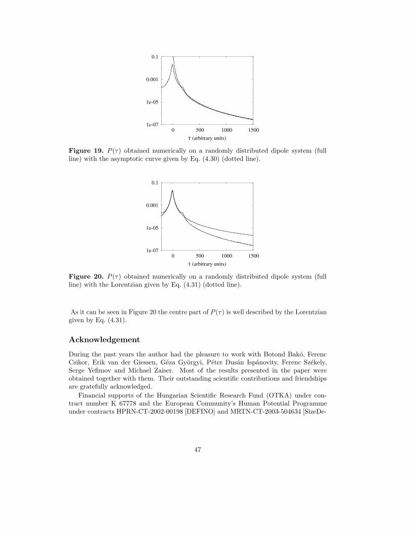
1e-07

1e-05

0.001

0.1

0 500 1000 1500

τ (arbitrary units)

Figure 19. P (τ) obtained numerically on a randomly distributed dipole system (fullline) with the asymptotic curve given by Eq. (4.30) (dotted line).

1e-07

1e-05

0.001

0.1

0 500 1000 1500

τ (arbitrary units)

Figure 20. P (τ) obtained numerically on a randomly distributed dipole system (fullline) with the Lorentzian given by Eq. (4.31) (dotted line).

As it can be seen in Figure 20 the centre part of P (τ) is well described by the Lorentziangiven by Eq. (4.31).

Acknowledgement

During the past years the author had the pleasure to work with Botond Bako, FerencCsikor, Erik van der Giessen, Geza Gyorgyi, Peter Dusan Ispanovity, Ferenc Szekely,Serge Yefimov and Michael Zaiser. Most of the results presented in the paper wereobtained together with them. Their outstanding scientific contributions and friendshipsare gratefully acknowledged.

Financial supports of the Hungarian Scientific Research Fund (OTKA) under con-tract number K 67778 and the European Community’s Human Potential Programmeunder contracts HPRN-CT-2002-00198 [DEFINO] and MRTN-CT-2003-504634 [SizeDe-

47

pEn] are also acknowledged.

Bibliography

[1] I. Kovacs and L. Zsoldos, Dislocations and Plastic Deformation, Pergamon Press,London (1973).

[2] Basinski S.J. and Basinski Z.S., Dislocations in Solids, ed. by F.R.N. Nabarro, North-Holland, Amsterdam, 1979

[3] Hirsh JP. Lothe J. Theory of dislocations, John Wiley and Sons, 1982

[4] Mughrabi H., Ungar T., Kienle W., M. Wilkens, Phil. Mag. 53, 793 (1986)

[5] Mughrabi H., Ackerman F., Herz K., in J. Fang (editor), Fatigue Mechanisms,Proc. of ASTM-NBS-NSF Symposium, ASTM-STP 675, 1979, p. 69.

[6] Kuhlmann-Wilsdorf D., van der Merwe J., Mat. Sci. Eng. 35, 79 (1982)

[7] Bassim M., Jesser W., Kuhlmann-Wilsdorf D., Wilsdorf H., Mat. Sci. Eng. 81,122 (1986)

[8] Kuhlmann-Wilsdorf D., Mat. Sci. Eng. A 113, 1 (1989)

[9] Holt D., Journal Appl. Phys. 41, 3179 (1970)

[10] Walgraef D., Aifantis E., J. Appl. Phys. 15, 688 (1985)

[11] Aifantis E., Mat. Sci. Eng. 81, 563 (1986)

[12] Walgraef D., Solid State Phenomena, 3-4, 77 (1988)

[13] Kratochvil J., Scripta Metall. Mater. 24, 891 (1990)

[14] Kratochvil J., Scripta Metall. Mater. 24, 1225 (1990)

[15] Kratochvil J., and Saxlova M., Scripta Met. Mater. 26, 113 (1993)

[16] Hahner P., Bay K., Zaiser M., Phys. Rev. Lett. 81, 2470 (1998)

[17] Zaiser M., Bay K., Hahner P., Acta mater. 47, 2463 (1999)

[18] Szekely F., Groma I., Lendvai J., Mat. Sci. Eng. A 309, 352 (2001)

[19] Szekely F., Groma I., Lendvai J., Scripta Mater 45, 55 (2001)

[20] Fleck N.A., Mller G.M., Ashby M.F. and Hutchinson J.W., Acta Mater. 42, 475(1994)

[21] McElhaney K.W., Vlassah JJ. and Nix W.D., J. Math. Res. 13, 1300 (1998)

[22] Aifantis E.C., J. Eng. Mater. Technol. 106, 326 (1984)

[23] Aifantis E.C., Int. J. Plast. 2, 211 (1987)

[24] Aifantis E.C., J. Mech. Behav. Mater. 5, 335 (1994)

[25] Fleck N.A. and Hutchinson J.W., J. Mech. Phys. Solids, 49, 2245 (2001)

[26] Gurtin M.E., J. Mech. Phys. Solids, 50, 5 (2002)

[27] Svendsen B., J. Mech. Phys. Solids, 50, 1297 (2002)

[28] Nicola L., van der Giessen E. and Needleman A., Journal of Applied Physics 93,5920 (2003)

[29] Kroner E., Z. Phys. 151, 504 (1958)

[30] E. Kroner, Continuum Theory of Defects, Physics of Defects, Eds. R. Balian et.all,North Holland, Amsterdam (1981).

[31] L.D. Landau, E.M. Lifsitz, Theory of Elasticity, Course of Theoretical Physics, vol7, Pergamon Press, Oxford (1986)

48

[32] Kosevich A.M. in Dislocations in Solids, ed. by F.R.N. Nabarro, North-Holland,Amsterdam, 1979

[33] Nye J.F. Acta. Mat. 1, 153 (1953)

[34] Burgers J.M. Proc. Kon. Nederl. Akad. Wetensch. 42, 293 and 378 (1939)

[35] Devincre B., and Condat M., Acta Metall. Mater. 40, 2629 (1992)

[36] Fivel M., Gosling T.,and Canova , Modell. Simul. Mater. Sci. Eng. 4, 581 (1996)

[37] Huang J.M., and Ghoniem N.M., Model. Simul. Mater. Sci. 11, 21 (2003)

[38] Singh B.N., Ghoniem N.M., and Trinkaus H. J. Nucl. Mater. 307, 159 (2002)

[39] Huang H.M., and Ghoniem N.M. Comp. Mater. Sci. 23, 225 (2002)

[40] Walgraef D., and Ghoniem N.M. Phys. Rev. B 65, art. no. 155304 (2002)

[41] Madec R., Devincre B., and Kubin L.P., Phys. Rev. Lett. 89, 255508 (2002)

[42] Madec R., Devincre B., and Kubin L.P. Scripta Mater 47, 689 (2002)

[43] Lemarchand C., Chaboche J.L., and Devincre B,. J. Phys IV 9, 271 (1999)

[44] Bulatov V., Abraham F.F., Kubin L., Devincre B., and Yip S., Nature 391, 669(1998)

[45] Cai W., Bulatov V.V., Chang J., Li J. and Yip S., Phil. Mag. A, 81, 1257 (2001).

[46] Lepinoux J., and Kubin L., Scripta Met. Mat. 21, 833 (1987)

[47] Gulluoglu A., and Hartly C., Modell. Simul. Mater. Sci. Eng. 1, 383 (1993)

[48] Gullouglu A., Srolovity D., LeSar R., and Lomdahl P., Scripta Met. 23, 1347 (1989)

[49] Ghoniem N., and Amodeo R., Phys. Rev. B 41, 6968 (1989)

[50] Groma I. and Pawley G.S., Philos. Mag. A 67 1459 (1993)

[51] Groma I. and Pawley G.S., Mat. Sci. Eng. A 164, 306 (1993)

[52] Van der Giessen E., and Needleman A., Model. Simul. Mater. Sci. Eng. 3, 689 (1995)

[53] Cleveringa H. H. M., V. der Giessen E.,and Needleman A., Acta mater. 45, 3163(1997)

[54] Cleveringa, H.H.M., Van der Giessen, E., and Needleman, Acta Mater. 45, 3163(1997)

[55] Cleveringa, H.H.M., Van der Giessen, E. and Needleman, A., International Journalof Plasticity 15, 837 (1999)

[56] Cleveringa, H.H.M., Van der Giessen, E. and Needleman, A., Phil. Mag. A79, 863(1999)

[57] A. Benzerga, Y. Brechet, A. Needleman and E. Van der Giessen Model. Simul. Mat.Sci. Eng. 12, 159 (2004)

[58] Groma I., Phys. Rev. B 56, 5807 (1997)

[59] Groma I. and Balogh P., Acta Mater. 47, 3647 (1999)

[60] Buchinger L. and Stanzl S., Phil. Mag. A50, 275 (1984)

[61] Zaiser M., Miguel M.C., Groma I., Phys Rev B 64, 224102 (2001)

[62] Groma I., Csikor FF., Zaiser M., Acta Mater. 51, 1271 (2003)

[63] Cleveringa, H.H.M., Van der Giessen, E. and Needleman, A., J. Physique IV, 83, 92(1998)

[64] Yefimov S., Groma I. and van der Giessen E. J. de Physique IV 11, 103 (2001)

[65] S. Yefimov, I. Groma and E. van der Giessen J. Mech. and Phys. Solids 52, 279(2004)

49

[66] Yefimov S. and van der Giessen E European Journal of Mechanics A/Solids 24, 183(2005)

[67] Yefimov S. and van der Giessen E. Int. J. of Solids Struct. 42, 3375 (2005)

[68] El-Azab A., Phys. Rev. B, 61, 11956, (2000)

[69] Hochrainer T. and Zaiser M., private communication

[70] Kratochvıl J. and Sedlacek R., Phys. Rev. B, 67, 094105 (2003)

[71] Groma I. and Bak B., Phys. Rev. B 58, 2969 (1998)

[72] Chandrasekhar S., Rev. Modern Phys. 15, 8 (1943)

[73] Csikor F.F. Groma I. Phys. Rev. B 70, 064106 (2004)

[74] Groma I.,Phys. Rev. B 57, 7535 (1998)

50