statistical modelling in stata 5: linear models

The linear ModelTesting assumptions

Statistical Modelling in Stata 5: Linear Models

Mark Lunt

Arthritis Research UK Epidemiology UnitUniversity of Manchester

30/10/2018


Structure

This WeekWhat is a linear model ?How good is my model ?Does a linear model fit this data ?

Next WeekCategorical VariablesInteractionsConfoundingOther Considerations

Variable SelectionPolynomial Regression


Statistical Models

All models are wrong, but some are use-ful.

(G.E.P. Box)

A model should be as simple as possible,but no simpler. (attr. Albert Einstein)


IntroductionParametersPredictionANOVAStata commands for linear models

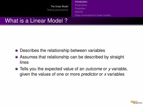
What is a Linear Model ?

Describes the relationship between variablesAssumes that relationship can be described by straightlinesTells you the expected value of an outcome or y variable,given the values of one or more predictor or x variables



Variable Names

Outcome PredictorDependent variable Independent variablesY-variable x-variablesResponse variable RegressorsOutput variable Input variables

Explanatory variablesCarriersCovariates



The Equation of a Linear Model

The equation of a linear model, with outcome Y and predictorsx1, . . . xp

Y = β0 + β1x1 + β2x2 + . . .+ βpxp + ε

β0 + β1x1 + β2x2 + . . .+ βpxp is the Linear Predictor

Y = β0 + β1x1 + β2x2 + . . .+ βpxp is the predictable part ofY .ε is the error term, the unpredictable part of Y .We assume that ε is normally distributed with mean 0 andvariance σ2.



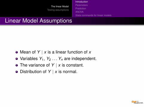
Linear Model Assumptions

Mean of Y | x is a linear function of xVariables Y1, Y2 . . . Yn are independent.The variance of Y | x is constant.Distribution of Y | x is normal.



Parameter Interpretation

Y

x

Y =

1

β1

β0

β1

β0 + x

β1 is the amount by which Y increases if x1 increases by 1, andnone of the other x variables change.

β0 is the value of Y when all of the x variables are equal to 0.



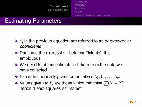
Estimating Parameters

βj in the previous equation are referred to as parameters orcoefficientsDon’t use the expression “beta coefficients”: it isambiguousWe need to obtain estimates of them from the data wehave collected.Estimates normally given roman letters b0,b1, . . . ,bn.Values given to bj are those which minimise

∑(Y − Y )2:

hence “Least squares estimates”



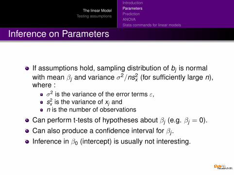
Inference on Parameters

If assumptions hold, sampling distribution of bj is normalwith mean βj and variance σ2/ns2

x (for sufficiently large n),where :

σ2 is the variance of the error terms ε,s2

x is the variance of xj andn is the number of observations

Can perform t-tests of hypotheses about βj (e.g. βj = 0).Can also produce a confidence interval for βj .Inference in β0 (intercept) is usually not interesting.



Inference on the Predicted Value

Y = β0 + β1x1 + . . .+ βpxp + ε

Predicted Value Y = b0 + b1x1 + . . .+ bpxp

Observed values will differ from predicted values becauseof

Random error (ε)Uncertainty about parameters βj .

We can calculate a 95% prediction interval, within whichwe would expect 95% of observations to lie.Reference Range for Y



Prediction IntervalY

1

x1

0 5 10 15 200

5

10

15



Inference on the Mean

The mean value of Y at a given value of x does notdepend on ε.The standard error of Y is called the standard error of theprediction (by stata).We can calculate a 95% confidence interval for Y .This can be thought of as a confidence region for theregression line.



Confidence IntervalY

1

x1

0 5 10 15 200

5

10

15



Analysis of Variance (ANOVA)

Variance of Y is∑

(Y−Y)2

n−1 =∑

(Y−Y)2+∑

(Y−Y)2

n−1

SSreg =∑(

Y − Y)2

(regression sum of squares)

SSres =∑(

Y − Y)2

(residual sum of squares)

Each part has associated degrees of freedom: p d.f for theregression, n − p − 1 for the residual.The mean square MS = SS/df .MSreg should be similar to MSres if no association betweenY and xF =

MSregMSres

gives a measure of the strength of theassociation between Y and x .



ANOVA Table

Source df Sum of Mean Square FSquares

Regression p SSreg MSreg =SSreg

pMSreg

MSres

Residual n-p-1 SSres MSres =SSres

(n − p − 1)

Total n-1 SStot MStot =SStot

(n − 1)



Goodness of Fit

Predictive value of a model depends on how much of thevariance can be explained.R2 is the proportion of the variance explained by the model

R2 =SSregSStot

R2 always increases when a predictor variable is addedAdjusted R2 is better for comparing models.



Stata Commands for Linear Models

The basic command for linear regression isregress y-var x-varsCan use by and if to select subgroups.The command predict can produce

predicted valuesstandard errorsresidualsetc.



Stata Output 1: ANOVA Table

F() F Statistic for the Hypothesis βj = 0 for all jProb > F p-value for above hypothesis testR-squared Proportion of variance explained by regression

= SSModelSSTotal

Adj R-squared (n−1)R2−pn−p−1

Root MSE√

MSResidual

= σ



Stata Output 1: Example

Source | SS df MS Number of obs = 11---------+------------------------------ F( 1, 9) = 17.99

Model | 27.5100011 1 27.5100011 Prob > F = 0.0022Residual | 13.7626904 9 1.52918783 R-squared = 0.6665---------+------------------------------ Adj R-squared = 0.6295

Total | 41.2726916 10 4.12726916 Root MSE = 1.2366



Stata Output 2: Coefficients

Coef. Estimate of parameter β for the variable in theleft-hand column. (β0 is labelled “_cons” for“constant”)

Std. Err. Standard error of b.t The value of b−0

s.e.(b) , to test the hypothesis thatβ = 0.

P > |t| P-value resulting from the above hypothesis test.95% Conf. Interval A 95% confidence interval for β.



Stata Output 2: Example

------------------------------------------------------------------------------Y | Coef. Std. Err. t P>|t| [95% Conf. Interval]

---------+--------------------------------------------------------------------x | .5000909 .1179055 4.241 0.002 .2333701 .7668117

_cons | 3.000091 1.124747 2.667 0.026 .4557369 5.544445------------------------------------------------------------------------------


Constant VarianceLinearityInfluential pointsNormality

Is a linear model appropriate ?

Does it provide adequate predictions ?Do my data satisfy the assumptions of the linear model ?Are there any individual points having an inordinateinfluence on the model ?



Anscombe’s Data

Y1

x10 5 10 15 20

0

5

10

15

Y2

x10 5 10 15 20

0

5

10

15

Y3

x10 5 10 15 20

0

5

10

15

Y4

x20 5 10 15 20

0

5

10

15



Linear Model Assumptions

Linear models are based on 4 assumptionsMean of Yi is a linear function of xi .Variables Y1, Y2 . . . Yn are independent.The variance of Yi | x is constant.Distribution of Yi | x is normal.

If any of these are incorrect, inference from regressionmodel is unreliableWe may know about assumptions from experimentaldesign (e.g. repeated measures on an individual areunlikely to be independent).Should test all 4 assumptions.



Distribution of Residuals

Error term εi = Yi − β0 + β1x1i + β2x2i + . . .+ βpxpi

Residual termei = Yi − b0 + b1x1i + b2x2i + . . .+ bpxpi = Yi − Yi

Nearly but not quite the same, since our estimates of βj areimperfect.Predicted values vary more at extremes of x-range (pointshave greater leverageHence residuals vary less at extremes of the x-rangeIf error terms have constant variance, residuals don’t.



Standardised Residuals

Variation in variance of residuals as x changes ispredictable.Can therefore correct for it.Standardised Residuals have mean 0 and standarddeviation 1.Can use standardised residuals to test assumptions oflinear modelpredict Yhat, xb will generate predicted valuespredict sres, rstand will generate standardisedresidualsscatter sres Yhat will produce a plot of thestandardised residuals against the fitted values.



Testing Constant Variance:

Residuals should be independent of predicted valuesThere should be no pattern in this plotCommon patterns

Spread of residuals increases with fitted valuesThis is called heteroskedasticityMay be removed by transforming YCan be formally tested for with hettest

There is curvatureThe association between x and Y variables is not linearMay need to transform Y or xAlternatively, fit x2, x3 etc. termsCan be formally tested for with ovtest



Residual vs Fitted Value Plot ExamplesY

x.000087 .99163

−1.81561

2.28352

(a) Non-constant variance

Y

x.000087 .99163

1.35659

10.5454

(b) Non-linear association



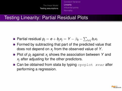
Testing Linearity: Partial Residual Plots

Partial residual pj = e + bjxj = Y − β0 −∑

l 6=j blxl

Formed by subtracting that part of the predicted value thatdoes not depend on xj from the observed value of Y .Plot of pj against xj shows the association between Y andxj after adjusting for the other predictors.Can be obtained from stata by typing cprplot xvar afterperforming a regression.



Example Partial Residual Plot

e( Y

2 | X

,x1

) +

b*x

1

x1

Residuals Linear prediction

4 14.099091

7



Identifying Outliers

Points which have a marked effect on the regressionequation are called influential points.Points with unusual x-values are said to have highleverage.Points with high leverage may or may not be influential,depending on their Y values.Plot of studentised residual (residual from regressionexcluding that point) against leverage can show influentialpoints.



Statistics to Identify Influential Points

DFBETA Measures influence of individual point on a singlecoefficient βj .

DFFITS Measures influence of an individual point on itspredicted value.

Cook’s Distance Measured the influence of an individual pointon all predicted values.

All can be produced by predict.There are suggested cut-offs to determine influentialobservations.May be better to simply look for outliers.



Y -outliers

A point with normal x-values and abnormal Y -value maybe influential.Robust regression can be used in this case.

Observations repeatedly reweighted, weight decreases asmagnitude of residual increases

Methods robust to x-outliers are very computationallyintensive.



Robust Regression

Y3

x1

Y3 LS Regression Robust Regression

5 10 155

10

15



Testing Normality

Standardised residuals should follow a normal distribution.Can test formally with swilk varname.Can test graphically with qnorm varname.



Normal Plot: ExampleS

tand

ardi

zed

resi

dual

s

Inverse Normal

Standardised Residuals Inverse Normal

−1.4619 1.43573−1.77998

1.61402

Sta

ndar

dize

d re

sidu

als

Inverse Normal

Standardised Residuals Inverse Normal

−1.48979 1.51139−1.48979

2.99999



Graphical Assessment & Formal Testing

Can test assumptions both formally and informallyBoth approaches have advantages and disadvantages

Tests are always significant in sufficiently large samples.Differences may be slight and unimportant.Differences may be marked but non-significant in smallsamples.

Best to use both

statistical modelling in stata 5: linear models

Documents