statistical methods in particle physics lecture 2nberger/teaching/ws11/lecture... · ifa⊂b,thenp...

Statistical Methodsin Particle Physics

Lecture 2October 17, 2011

Winter Semester 2011 / 12

Silvia Masciocchi, GSI [email protected]

mailto:[email protected]

Statistical Methods, Lecture 2, October 17, [email protected] 2

Outline

● Probability● Definition and interpretation● Kolmogorov's axioms

● Bayes' theorem

● Random variables● Probability density functions (pdf)● Cumulative distribution function (cdf)


Uncertainty

In particle physics there are various elements of uncertainty:

● theory is not deterministic● quantum mechanics

● random measurement errors● present even without quantum effects

● things we could know in principle but don’t● e.g. from limitations of cost, time, ...

We can quantify the uncertainty using PROBABILITY


Some ingredients

● Set of elements S

● Subsets A, B, … of set S

● : A or B (union of A and B)

● : A and B (intersection of A and B)

● : not A (complementary of A)

● : A contained in B

● P(A): probability of A

A∪B

A∩B

AA⊂B

A

S

A

A

B

AA

B

BA


A definition of probability

Kolmogorov's axioms (1933)

1.

2. P(S) = 1

3.

For all A⊂S, PA≥0

If A∩B=0, thenPA∪B=PAPB

A

B

S

Normalized

Additive

Positive definite


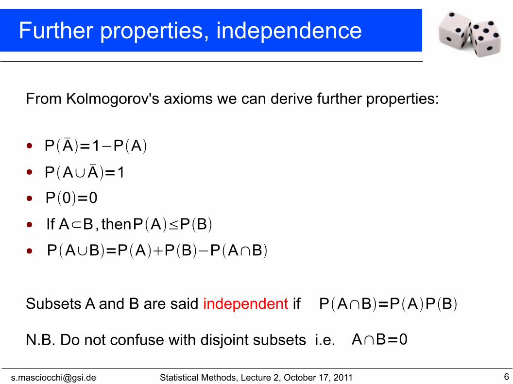
Further properties, independence

From Kolmogorov's axioms we can derive further properties:

●

●

●

●

●

Subsets A and B are said independent if

N.B. Do not confuse with disjoint subsets i.e.

P A=1−PA

PA∪A=1

P0=0

If A⊂B, thenPA≤PB

PA∪B=PAPB−PA∩B

PA∩B=PAPB

A∩B=0


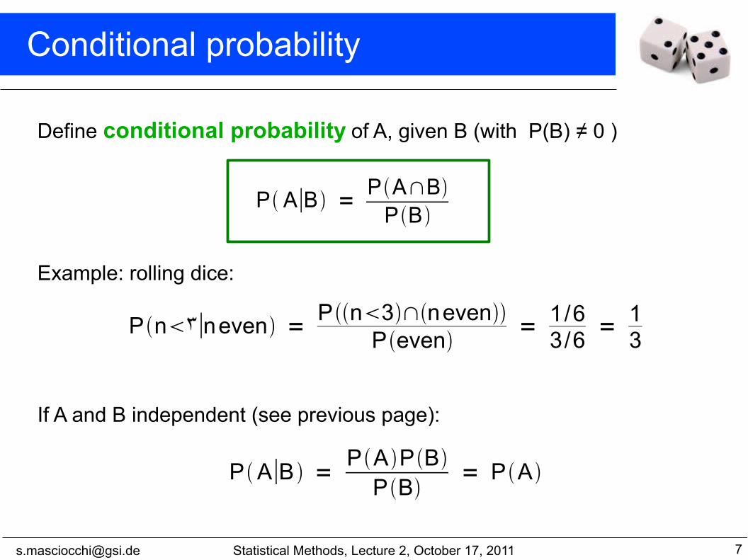
Conditional probability

Define conditional probability of A, given B (with P(B) ≠ 0 )

Example: rolling dice:

If A and B independent (see previous page):

P A∣B = PA∩BPB

Pn3∣neven = Pn3∩nevenPeven

= 1 /63 /6

= 13

PA∣B =PAPB

PB= PA


Bayes' theorem

P A∣B = PA∩BPB

PB∣A = PB∩A PA

From the definition of conditional probability we have:

and

But , so:

First published (posthumously) by theReverend Thomas Bayes (1702−1761)An essay towards solving a problem in the doctrine of chances,

Philos. Trans. R. Soc. 53c(1763) 370; reprinted in Biometrika, 45 (1958) 293.

PA∩B=PB∩A

P A∣B = PB∣A PAPB

Bayes' Theorem


The law of total probability

Consider a subset B of the sample space S,divided into disjoint subsets Ai

such that ∪i Ai = S :

→

→

→

Bayes' theorem

becomes:

B

Ai

S

B∩AiB = B∩S = B∩ ∪i A i = ∪iB∩Ai

PB = P ∪iB∩A i = ∑iPB∩A i

PB = ∑iPB∣A i PA i Law of total probability

P A∣B = PB∣A PA

∑iPB∣A iPA i


Example: rare disease (1)

Suppose the probability (for anyone) to have the disease A is:

Consider a test for that disease. The result can be 'pos' or 'neg' :

Suppose your result is 'pos'. How worried should you be?

PA = 0.001Pno A = 0.999

Ppos∣A = 0.98Pneg∣A = 0.02

Ppos∣no A = 0.03Pneg∣no A = 0.97

← probabilities to (in)correctly Identify an infected person

← probabilities to (in)correctly Identify an infected person



The probability to have the disease A, given a 'pos' result is:

PA∣pos =



The probability to have the disease A, given a 'pos' result is:

i.e. you’re probably OK!Your viewpoint: my degree of belief that I have disease A is 3.2%Your doctor’s viewpoint: 3.2% of people like this will have disease A

PA∣pos =Ppos∣A PA

Ppos∣A PA Ppos∣no A Pno A

= 0.98×0.0010.98×0.0010.03×0.999

= 0.032


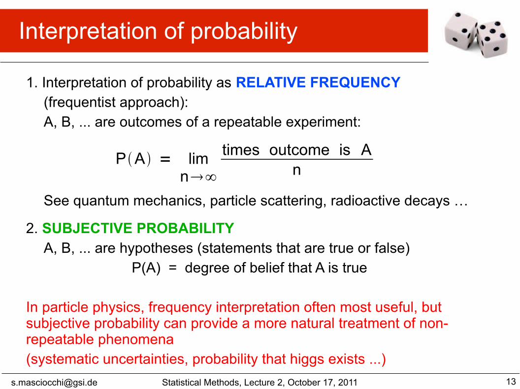
Interpretation of probability

1. Interpretation of probability as RELATIVE FREQUENCY(frequentist approach):A, B, ... are outcomes of a repeatable experiment:

See quantum mechanics, particle scattering, radioactive decays …

2. SUBJECTIVE PROBABILITYA, B, ... are hypotheses (statements that are true or false) P(A) = degree of belief that A is true

In particle physics, frequency interpretation often most useful, but subjective probability can provide a more natural treatment of non-repeatable phenomena (systematic uncertainties, probability that higgs exists ...)

PA = limn∞

times outcome is An


Frequentist statistics

In frequentist statistics, probabilities are associated only withthe data, i.e., outcomes of repeatable observations

Any given experiment can be considered as one of an infinite sequence of possible repetitions of the same experiment, each capable of producing statistically independent results: Perform experiment N times in identical trials; assume event E occurs k times, then

BUT:● Does the limit converge? How large needs N to be?● What means identical condition? Can 'similar' be sufficient? ● Not applicable for single events

PE = limN∞

k /N


Bayesian probability

In Bayesian statistics, use subjective probability for hypotheses(degree of belief that an hypothesis is true):

PH∣x =P x∣HH

∫Px∣H HdH

Probability of the data assuminghypothesis H (the likelihood)

Prior probability (before seeing the data)

Posterior probability (after seeing the data) Normalization involves sum over all

possible hypothesis

Bayes’ theorem has an “if-then” character: If your prior probabilities were π(H), then it says how these probabilities should change in the light of the data.

No general prescription for priors (subjective!)


Back to Bayes' theorem

P A∣B = PB∣A PAPB

Now take: A = theory, B = data:

P theory∣data = P data∣theoryPtheoryPdata

Likelihood Prior

EvidencePosterior


Exercises

1. Show that:

2. A beam of particles consists of a fraction 10-4 electrons and the rest photons. The particles pass through a double-layered detector which gives signals in either zero, one or both layers. The probabilities of these outcomes for electrons (e) and photons (γ) are:

(a) what is the probability for a particle detected in one layer only to be a photon?(b) what is the probability for a particle detected in both layers to be an electron?

PA∪B=PAPB−PA∩B

P0∣e =0.001P1∣e=0.01

P2∣e=0.989

P0∣=0.99899P1∣=0.001

P2∣=10−5


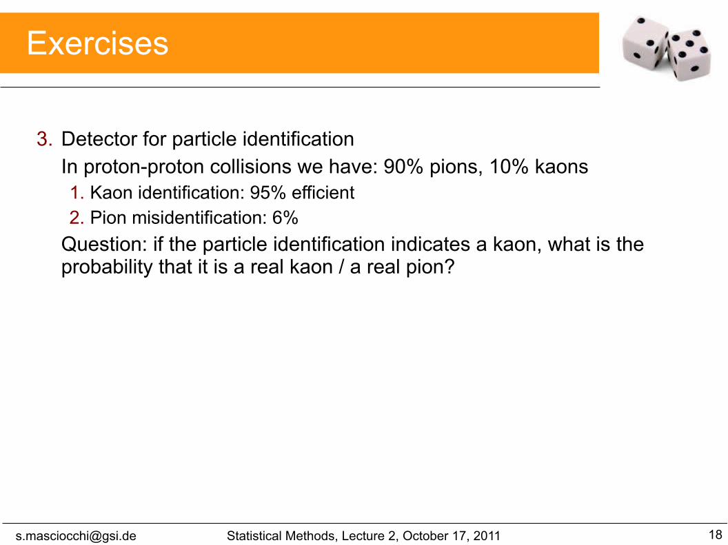
Exercises

3. Detector for particle identificationIn proton-proton collisions we have: 90% pions, 10% kaons1. Kaon identification: 95% efficient2. Pion misidentification: 6%

Question: if the particle identification indicates a kaon, what is the probability that it is a real kaon / a real pion?


Hints

1. Express AUB as the union of three disjoint sets

2.

3. PA∣B =PB∣A PA

PB∣A PAPB∣no A [1−PA]


Random variables

A random variable is a variable whose value results from a measurement on some type of random process.

Formally, it is a function from a probability space, typically to the real numbers, which is measurable.

Intuitively, a random variable is a numerical description of the outcome of an experiment e.g., the possible results of rolling two dice: (1, 1), (1, 2), etc.

Random variables can be classified as: ● discrete (a random variable that may assume a finite number of values)● continuous (a variable that may assume any numerical value in an

interval or collection of intervals).


Probability density functions

Suppose outcome of experiment is continuous value x:

→ f(x) = probability density function (pdf)With:

Note:● f(x) ≥ 0● f(x) is NOT a probability ! It has dimension 1/x !

Px found in [x ,xdx ] = f x dx

∫−∞

∞f xdx=1 Normalization

(x must be somewhere)


Probability density functions

Otherwise, for a discrete outcome xi, with i=1,2,... :

Pxi=pi

∑iPxi=1

Probability mass function

x must take on one of its possible values


Cumulative distribution function (cdf)

Given a pdf f(x'), probability to have outcome less then or equal to x, is:

∫−∞

xf x 'dx ' = Fx

Cumulative distribution function


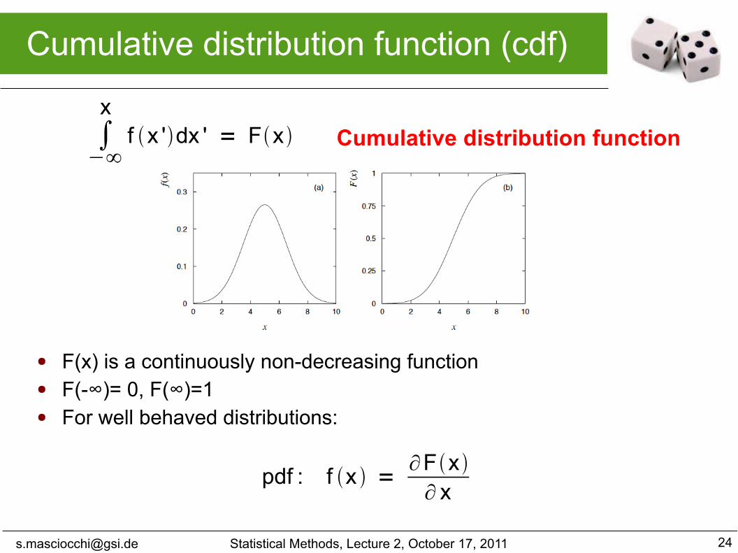
Cumulative distribution function (cdf)

∫−∞

xf x 'dx ' = Fx Cumulative distribution function

● F(x) is a continuously non-decreasing function● F(-∞)= 0, F(∞)=1● For well behaved distributions:

pdf : f x =∂Fx ∂ x


Exercise

1. Given the probability density function:

- compute the cdf F(x)- what is the probability to find x > 1.5 ?- what is the probability to find x in [0.5,1] ?

f x = { |1-x| for x in [0,2]0 elsewhere


Histograms

A probability density function can be obtained from a histogram at the limit of:

● Infinite data sample● Zero bin width● Normalized to unit area

N = number of entriesΔx = bin width

f x =Nx n x


Wrapping up lecture 2, next time

This lecture:● Abstract properties of probability● Axioms ● Interpretations of probability● Bayes' theorem● Random variables● Probability density function● Cumulative distribution function

Next time:● Expectation values● Error propagation● Catalog of pdfs

statistical methods in particle physics lecture 2nberger/teaching/ws11/lecture... · ifa⊂b,thenp...

Documents