statistical methodology to make early estimates of motor - nhtsa

NHTSA’s National Center for Statistics and Analysis 1200 New Jersey Avenue SE., Washington, DC 20590

TRAFFIC SAFETY FACTSResearch Note

DOT HS 811 123 Summary of Statistical Findings November 2010

Statistical Methodology to Make Early Estimates of Motor Vehicle Traffic FatalitiesHighlightsBeginning with the third quarter of 2008, NHTSA began making quarterly projections of motor vehicle traffic fatalities. The latest such projection was made by NHTSA recently (DOT HS 811 403, September 2010) and showed that fatalities in motor vehicle traffic crashes during the first six months (January through June) of 2010 are projected to decline by about 9.2 percent as com-pared to the same time period in 2009. The estimated month-to-month fatality counts for 2010 and reported FARS fatalities from January through June during 2008 and 2009 are depicted in Figure 1. This Research Note details the underlying data and the statistical methodol-ogy that was used to estimate fatalities during the first half of 2010. This methodology and data will be used to make future estimates and will be continuously evalu-ated to make refinements to the estimation process.

Figure 1Reported Fatalities in 2008–2009 and Projected Fatalities In 2010, January to June

1. IntroductionThe National Highway Traffic Safety Administration and the highway safety community have an essential need for “real-time” or “near-real-time” data on the number of fatalities resulting from motor vehicle traffic crashes. This data is required to provide timely infor-mation to Congress, to report on progress toward meet-ing agency and Department goals, to assist States in their safety programs, and to inform the public about the state of highway safety. NHTSA’s existing data pro-grams, the Fatality Analysis Reporting System (FARS) and the National Automotive Sampling System (NASS), were designed to provide a detailed annual account-ing of characteristics of motor vehicle crashes. Because considerable time is necessary to obtain the data these systems require, producing real-time crash fatality data from them is not currently possible. With this emerg-ing data need in mind, Congress authorized NHTSA to develop FastFARS – a fatality reporting system using the FARS infrastructure, but which must provide near-real-time accounting of traffic fatality counts. NHTSA was mandated to develop FastFARS without interrupt-ing the collection of the detailed information in FARS. The success of FastFARS depends on three factors: (1) Reliable and timely notification of crash fatalities within each State; (2) Timely and accurate reporting of fatality counts by each State to NHTSA; and (3) com-pilation of State fatality counts into a national total. FastFARS operated in a prototype mode in 2006 and 2007 and in a production mode in 2008. While the time-liness and accuracy of Fast-FARS have considerably improved since its inception in 2006, there still remain under-reporting and other non-response problems in various States. To address this issue, NHTSA has devel-oped a statistical procedure that is a combination of adjusting the fatality data reported through Fast-FARS and other independent sources to date in 2010 and

3,500

3,000

2,500

2,000

1,500Jan Feb Mar Apr May Jun

2008 2009 2010*

*Estimates, NHTSA DOT HS 811 403

2


modeling the adjusted data to estimate fatalities. This Research Note describes the adjustment procedures as well as the modeling procedure—Time Series Cross Sectional Regression (TSCSR)—that was used to esti-mate the fatalities in the United States for the first six months of 2010.

2. DataThe data used in this analysis is from several sources such as FARS, FastFARS and monthly fatality counts (MFCs), as described below.

FARS: FARS is a census of fatal traffic crashes within the 50 States, the District of Columbia, Puerto Rico and the U.S. Virgin Islands. To be included in FARS, a crash must involve a motor vehicle traveling on a trafficway and result in the death of a person (occupant of a vehicle or a non-occupant) within 30 days of the crash. Fatality counts, by month, as reported to NHTSA’s FARS files from January 2003 to December 2009 are used. Fatalities in Puerto Rico or the U.S. Virgin Islands are not part of the national estimates.

FastFARS (Early Notification): The FastFARS program is designed as an Early Fatality Notification System to capture data from States more rapidly and in real-time. It provides near-real-time notification of fatalities from all jurisdictions reporting to FARS by electronically transmitting fatal crash data. This system is continu-ously cumulated and updated. In this Research Note, FastFARS data from January 2006 to June 2010 were used from a snapshot taken on August 24, 2010.

Figure 2 shows the cumulative percentage of all crash fatality counts reported within the first 30 days for this recent Fast-FARS file (snapshot). The figure shows that the notification into the FastFARS data system has been steadily improving. In fact, in 2006 while about 80 per-cent of the traffic fatalities were reported by 30 days from the time of the crash, just about 90 percent of the traffic fatalities were reported within 30 days in 2010. The line for 2010 is based only on crashes reported to date, and there may still be fatal crashes that occurred in 2010 that have not yet been reported into Fast-FARS.

Monthly Fatality Counts (MFC): The MFC data pro-vide monthly fatality counts by State through sources that are independent from the FastFARS or FARS sys-tems. MFCs from January 2003 to June 2010 are used. MFCs are reported mid-month for all prior months of the year.

Figure 2Cumulative Percentage of All Crash Fatality Counts Reported Within the First 30 Days in FastFARS in 2006–2010 Data Years

100%90%80%70%60%50%40%30%20%10%

0%0 2 4 6 8 10 12 14 16 18 20 22 24 26 28 30

Number of Days After Crash for Notification

% o

f Fin

al F

atal

ities

2006 2007 2008 2009* 2010*

*2009 and 2010 FARS data are still being reported

3. MethodologyIn the estimation of fatalities in each month (January–June) of 2010, the modeling procedure uses the rela-tionship among FARS, MFC and FastFARS. The fatality counts from MFCs are updated every month and become stable after a certain time. Similarly, the fatality counts from FastFARS are continuously updated due to real-time notification and stabilize after a certain lag time. However, historically FastFARS and MFCs pro-duce marginally different monthly fatality counts from FARS even after they become stable. Also, the differ-ence of FastFARS and MFC from FARS fluctuates over time. Due to this reason, the procedure of estimating traffic fatalities consists of two steps, adjustment of data based on reporting levels followed by modeling using the adjusted data. The TSCSR procedure in SAS was used in the modeling procedure, the details of which can be found in the SAS (1999).

3.1 Adjustment ProceduresSince the two datasets, MFC and FastFARS, which are used as predictor variables in the modeling procedure, have not been finalized for 2009 and 2010, they need to be adjusted (inflated) based on historical reporting pat-terns. The details of the adjustment procedures for MFC and FastFARS are provided in the following sections.

3


3.1.1 Adjustment of MFCThe MFCs in crashes that occurred during CY (crash year), CM (crash month), and reported during RY (reporting year) and RM (reporting month), are labeled as: CMCY

RMRYMFC ,, . The most recent MFC snapshot for CY =

2010 and CM = Jan., Feb.,…, Jun., was reported on RY = 2010 and RM = Aug. The 2010 MFCs will continually be updated until late 2011 and hence the “final” fatal-ity counts for CMCY

AugRMRYMFC ,2010,2010

=== (CM = Jan., Feb., …, Jun.)

are estimated by making an inflation based on report-ing patterns in previous years. Historical MFC data is available each year from CY1 to CY2 (CY2 > CY1). The starting file (snapshot) is RM1 = Nov, the most recent reporting month (for each year from CY1 to CY2). The final file (snapshot) with the last reporting year (RY2) and the last reporting month (RM2) for that crash year (CY) is CMCY

RMRYMFC ,2,2 . Generally, RY2 = CY+1 and RM2 =

December in MFC dataset. Then, the percentage change (i.e., the inflation rate) between these two files (snap-shots) for each crash month of the year is given by equa-tion (1) below,

CMCYRMRY

CMCYOctRMCYRY

CMCYRMRYCY

CMMFC

MFCMFC

,2,2

,1,1

,2,2 )(

%==−

= (1)

where CY = CY1, CY1+1, CY1+2, … , CY2, CM = Jan., Feb., …, Jun.

There are potentially two approaches can be followed for the next step adjustment. The first approach is to take the average rate of years between CY1 and CY2:

)112(

%

%

2

1+−

=><∑=

=CYCY

CYCY

CYCY

CYCM

CM

(2)

Then, the “final” adjusted (inflated) crash fatality counts for the initial raw counts CMCY


=== is,

)%1(_

,2010,2010,2010

,2010 ><−=

====

==CM

CMCYAugRMRYCMCY

AugRMRY

MFCMFCAdjusted (3)

where CM = Jan., Feb., …, Jun.

In the calculations of the average rate < %CM > in (2), the adjustment (inflation) rate shows an overall decreasing trend as the crash year CY increases from CY1 = 2003 to CY2 = 2008 for every crash month, implying that the reporting to the MFC system has been improving (the lag time between the crash event and the data entered into the system is getting shorter). Consequently, a second approach is to use a single ( CY

CM% ) as computed in (1) of the most recent year data to do this adjustment (inflation) for CMCY


=== in (3). In this study, the

second approach is adopted by calculating the infla-tion rate based on the 2008 MFC data and then this rate is applied to adjust 2009 and 2010 MFC crash fatality counts, as 2008 is the most recent year for which the final MFC data has been reported.

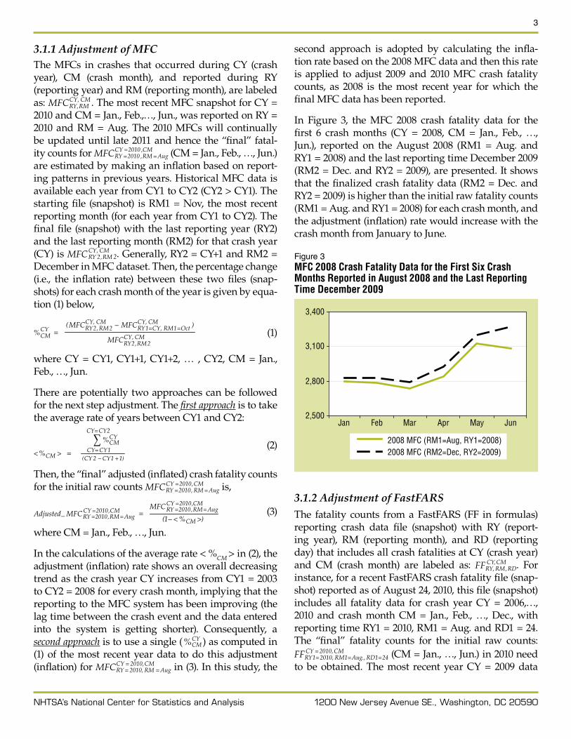
In Figure 3, the MFC 2008 crash fatality data for the first 6 crash months (CY = 2008, CM = Jan., Feb., …, Jun.), reported on the August 2008 (RM1 = Aug. and RY1 = 2008) and the last reporting time December 2009 (RM2 = Dec. and RY2 = 2009), are presented. It shows that the finalized crash fatality data (RM2 = Dec. and RY2 = 2009) is higher than the initial raw fatality counts (RM1 = Aug. and RY1 = 2008) for each crash month, and the adjustment (inflation) rate would increase with the crash month from January to June.

Figure 3MFC 2008 Crash Fatality Data for the First Six Crash Months Reported in August 2008 and the Last Reporting Time December 2009

2,500

2,800

3,100

3,400

Jan Feb Mar Apr May Jun

2008 MFC (RM1=Aug, RY1=2008)2008 MFC (RM2=Dec, RY2=2009)

3.1.2 Adjustment of FastFARSThe fatality counts from a FastFARS (FF in formulas) reporting crash data file (snapshot) with RY (report-ing year), RM (reporting month), and RD (reporting day) that includes all crash fatalities at CY (crash year) and CM (crash month) are labeled as: CMCY

RDRMRYFF ,,, . For

instance, for a recent FastFARS crash fatality file (snap-shot) reported as of August 24, 2010, this file (snapshot) includes all fatality data for crash year CY = 2006,…, 2010 and crash month CM = Jan., Feb., …, Dec., with reporting time RY1 = 2010, RM1 = Aug. and RD1 = 24. The “final” fatality counts for the initial raw counts:

CMCYRDAugRMRYFF ,2010

241.,1,20101=

=== (CM = Jan., …, Jun.) in 2010 need to be obtained. The most recent year CY = 2009 data

4


was used to calculate the adjustment (inflation) rate ( CMCY

RDRMRY,

,,% ) (with the same CM1, RM1 and RD1 as in CY = 2010), and then used to adjust the 2010 FastFARS to get the “final” fatality counts for CMCY

Aug., RD1=24RMRYFF ,20101,20101

=== .

The adjustment procedure is similar to the one in MFC. In Figure 4, based on a recent FastFARS file (snapshot) generated on 08/24/2010, the FastFARS 2009 crash fatal-ity data for the first 10 crash months (CY = 2009, CM = Jan., Feb., …, Jun.), reported on the 2009 (RD1 = 24, RM1 = Aug. and RY1 = 2009) and the late reporting time 2010 (RD2 = 24, RM2 = Aug. and RY2 = 2010), are presented. It shows that the finalized crash fatality data (RD2 = 24, RM2 = Aug. and RY2 = 2010) is higher than the initial raw fatality counts (RD1 = 24, RM1 = Aug. and RY1 = 2009) for each crash month, and the adjustment (infla-tion) rate would increase with the crash month from January to June. This represents the first adjustment to the FastFARS data.

Figure 4FastFARS 2009 Crash Fatality Data for the First Six Crash Months Reported in August 2009 and the Last Reporting Time August 2010

2,000

2,400

2,800

3,200

3,600

4,000


2009 FF (RD1=24, RM1=Aug, RY1=2009)

2009 FF (RD2=24, RM2=Aug, RY2=2010)

Figure 5MFC, Adjusted MFC, FastFARS, and Adjusted FastFARS For the First Six Months in 2010

1,800

2,200

2,600

3,000

3,400

3,800


FF FF - Adj.MFC MFC-Adj.

3.2 Modeling ProcedureIn order to estimate the monthly traffic fatality counts of 2010, Time Series Cross Section Regression (TSCSR), was applied to analyze the data with cross-sectional values (by NHTSA Region) and time series, where FARS, and the adjusted MFC and FastFARS are used as predictor variables in the modeling. A TSCSR model used for fatality prediction is denoted as

MmandruMFCFFFARS

rm

rmrmrm

...,,2,106...,,2,1,210

==+++= βββ

(4)

where FARSrm is FARS counts of regions r for month m FFrm is adjusted fatality counts from FastFARS of region r for month m, and MFCrm is adjusted fatality counts from MFC of region r for month m and where M is the length of the time series for each cross-section. In this study, when FastFARS is included in the model, time series of January 2006 to August 2010 data is used, M = 56 due to the availability of FastFARS. (or time series of January 2003 to August 2010 data is used, M = 92, which depends on the predictor variables of TSCSR models) and the number of time points across all 10 Regions are the same, that is, this data is balanced (Fuller & Battese, 1974). In the subsequent analysis, the adjusted FastFARS and MFC are denoted as FastFARS and MFC, respec-tively. In this model, the variance components urm in (1) consist of the individual, time-specific random effects and error disturbances and are specified as

Mmtandrevu rmmrrm ...,,110...,,2,1, ===++= ε (5)

where vr and em have a 0 mean and constant variances, σv

2 and σe2 , respectively and itε is a error term with

3.1.3 Results of AdjustmentsAs an example, based on one recent MFC and FastFARS data file (snapshot), the initial raw fatality counts and the adjusted “final” fatality counts for MFC and FastFARS for the first six crash month of the crash year 2010, are shown in Figure 5. These results confirm the expecta-tion that the final adjusted (inflated) number is higher than the initial raw fatality counts for each crash month, and the adjustment (inflation) rate increases with the crash month from January to June, for both MFC and FastFARS datasets.

5


,0 and for)( =rmE ε 2' )( εσεε =mrrmE 'rr ≠ . The parameters

are efficiently estimated using the generalized least squares (GLS) method which involves estimating the variance components first and using the estimated covariance matrix thus obtained. Refer to Fuller and Battese (1974) for details.

Model SelectionIn the TSCSR model, the variables adjusted MFC and adjusted FastFARS are considered. Table 1 shows three different combinations of predictors considered for a TSCSR model where data time points used are shown respectively. For more details, refer to the appendix.

Table 1Combination of Predictors in Modeling

Model (data time period)

Predictor Model Coefficients in (1)FF MFC

Mod 1 (Jan 06 – Jun 10) 3 β1≠0; β2=0

Mod 2 (Jan 03 – Jun 10) 3 β1=0; β2≠0

Mod 3 (Jan 06 – Jun 10) 3 β1≠0; β2=0

All three fitted TSCSR models considered in this analy-sis fit the data well with the Buse R-squared measure (R2) greater than 0.9, which is the most appropriate goodness-of-fit measure for models estimated using GLS, (Buse 1973). In other words, the six fitted models of using different predictor variables explain the his-torical data from FARS well. Under the assumption that the past relationship among dependent variables (fatality counts from FARS) and predictor variables (MFC and FastFARS) also holds in 2010, fatality counts of each month of 2010 are estimated by using the fitted models. When MFC and FastFARS are already included in a TSCSR model both MFC (p-value < 0.0001) and FastFARS (p-value = 0.08) are statistically significant even when the other variable is already in the model. For these reasons, the fitted model 3 (R2 = 0.9983) of including MFC and FastFARS as predictor variables is used for the national estimate of fatality counts of 2010.

4. Results

4.1. Estimated fatalities during 2010 (January–June)The estimates from this fitted model show 14,996 fatali-ties for the 6-month period from January to June 2010 as shown in Table 2. Fatalities during all six months declined as compared to the fatalities in the corre-sponding months in 2009. The biggest decline to date

in 2010 was an almost 15-percent decline in February, followed by about a 13-percent decline in January. The smallest decline of 4.5 percent was estimated for April 2010. Further details as well as fatality rates per 100 Million VMT have already been published by NHTSA in a separate document (DOT HS 811 403, Early Estimate of Traffic Fatalities during the First Six Months of 2010).

Table 2National Estimate of Fatalities of 2010 and Its Comparison With Fatality Counts From FARS in 2009

MonthFatalities from FARS in 2009*

Estimate of fatalities of 2010

Difference (2010–2009) (%)

Jan 2,608 2,275 -12.8%

Feb 2,351 2,010 -14.5%

Mar 2,580 2,402 -6.9%

Apr 2,867 2,739 -4.5%

May 3,044 2,809 -7.7%

June 3,059 2,761 -9.7%

Total 16,509 14,996 -9.2%

*FARS annual file in 2009

5. Model ValidationIn late 2008, during the development of this model to estimate fatalities in 2008, NHTSA ran some validation tests on FARS data that was already reported (2007). In order to validate the TSCSR model that includes the two predictor variables (MFC and FastFARS), the data was divided into two sets. The data prior to July 2007 (data A) was used to fit a model to predict the data after July 2007 (data B) in order to validate the model. When the simulated estimates and the corresponding actual fatality counts from FARS for the latter half of 2007 are compared, their differences are marginal, as indicated in Table 3.

Table 3Model Validation (Fatality Count From FARS in 2007 and Estimate of Fatalities)

MonthFatalities from FARS in 2007*

Estimate of fatalities

Difference (Estimate-FARS) (%)

July 3,800 3,808 0.2%

Aug 3,653 3,672 0.5%

Sept 3,562 3,566 0.1%

Oct 3,569 3,601 0.9%

Nov 3,322 3,358 1.1%

Dec 3,235 3,263 0.9%

Total 21,141 21,270 0.6%

*FARS annual file in 2007

6


Since 2008, NHTSA has been making a series of projec-tions to estimate fatalities for the first six months, nine months, and the full year. FARS data have since been reported for these time periods and this presents an opportunity to evaluate the estimates with the actual reported data. Table 4 shows the comparison between the projections and the reported data.

Table 4Model Validation (Reported Fatality Count From FARS and Estimate of Fatalities)

Time Period Estimated Reported Difference (%)

2008 (9 Months) 31,110 31,193 -0.3%

2008 (Full Year) 37,313 37,423 -0.3%

2009 (6 Months) 16,626 16,509* 0.7%

2009 (9 Months) 25,576 25,603* -0.1%

2009 (Full Year) 33,963 33,808* 0.5%

2010 (6 Months) 14,996 n/a n/a

*Annual Report File, Final File will be available late 2010

6. ConclusionNHTSA has applied the TSCSR procedure on adjusted data reported to date in FastFARS as well as using inde-pendent polls of MFCs to estimate fatality counts for the first six months of 2010. The estimates show that fatalities, when compared to the corresponding month in 2009, fell in each month from January through June. Overall, fatalities were down 9.2 percent for the first six months combined. Data reported through FARS will be available in fall of 2011.

7. References1. SAS/ETS(R) (1999). 9.2 User’s Guide, Cary, NC: SAS

Institute Inc.

2. Fuller, W. A., & Battese, G. E. (1974). Estimation of Linear Models with Crossed-Error Structure, Journal of Econometrics, 2, 67–78.

3. Buse, A. (1973). Goodness of Fit in Generalized Least Squares Estimation, American Statistician, 27, 106–108.

4. Brockwell, P. J., & Davis, R. A. (1996). Introduction to Time Series and Forecasting. New York: Springer-Verlag.

5. Fuller, W. A. (1962). Introduction to Statistical Time Series, 2nd ed. New York: John Wiley and Sons.

6. Schwarz, G. (1978). Estimating the dimension of a model. Annals of Statistics, 6(2), 461–464.

8. Appendix

8.1. Alternative Methodologies ConsideredIn 2008, as an alternative approach, the Auto Regressive Integrated Moving-Average (ARIMA) model includ-ing input time series, also called the ARIMAX model (Brockwell & Davis, 1996, or Fuller, 1996), was consid-ered for predicting the fatality counts in 2008. Note that the data without cross-sectional information is used in the ARMIAX modeling and more coefficients are esti-mated when this approach is compared with the TSCSR model. For example, the Bayesian Information Criterion (BIC) (Schwarz, 1978) here picked the ARIMAX (3,0,3) model, i.e., six more coefficients were estimated. Table 5 and Figure 6 show that the estimates from the ARIMAX model including MFC and FastFARS are close enough to those from the TSCSR model and fall within the 95 percent C.I.

The TSCSR modeling technique presented in this Research Note was chosen over the ARIMAX technique due to the sparseness (only three years) of known data points available to build the model. In future months, with more data points, it is envisioned that the esti-mation procedure will transition to a more traditional ARIMAX solution.

Table 5National Estimate of Crash Fatalities of 2008

MonthTSCSR

(MFC,FF)ARIMAX

(MFC, FF)95% Confidence Limits

of ARIMAX

Jan 2,816 2,803 2,781 2,824

Feb 2,805 2,797 2,772 2,822

Mar 2,804 2,795 2,769 2,822

Apr 2,935 2,927 2,900 2,954

May 3,212 3,205 3,178 3,232

June 3,291 3,285 3,257 3,312

July 3,287 3,281 3,253 3,308

Aug 3,612 3,607 3,580 3,635

Sept 3,075 3,067 3,039 3,095

Oct 3,273 3,267 3,239 3,295

Total 31,110 31,033 30,769 31,297

7


Figure 6Estimates of Fatality Counts of 2008 From TSCSR and ARIMAX With 95% C.I.

2,700

2,900

3,100

3,300

3,500

3,700

3,900

Jan

Feb

Mar Apr MayJu

ne July

Aug Sept

Oct

TSCSR

ARIMAX

Lower C.L.

Upper C.L.

8.2. Alternative Data Considered for ModelingMonthly Gasoline Consumption: The MGC is an esti-mate of total gasoline that is sold or delivered by the prime supplier (average consumption per day [unit: 1,000 gallons]). This information is provided by the Energy Information Administration for every State and the District of Columbia. Initially, for evaluating vari-ous forecasting models, the MGC from January 2003 to September 2008 were used. Figure 7 presents the

cyclical nature of traffic fatalities as well as gasoline consumption with the peak in fatalities and gasoline consumption occurring in the summer months and the lows in the winter months. However, MGC was not at all significant in predicting fatalities when FF and MFC were included in the model, as they are proxies of the fatalities themselves. Hence, MGC was dropped from further models.

Figure 7Monthly Gasoline Consumption and Traffic Fatalities

0

500

1,000

1,500

2,000

2,500

3,000

3,500

4,000

4,500

5,000

Jan-

07M

ay-0

7Se

p-07

Jan-

08M

ay-0

8Se

p-08

Jan-

09M

ay-0

9Se

p-09

Jan-

10M

ay-1

0Se

p-10

Jan-

11M

ay-1

1Se

p-11

340,000

346,000

352,000

358,000

364,000

370,000

376,000

382,000

388,000

394,000

400,000

Fata

litie

s

Gaso

line

Cons

umpt

ion

Fatalities Gasoline Consumption

8.3. Data Used in Various ModelsTable 6Various Models Evaluated During Development of Methodology to Estimate 2010 Fatalities (Six Month Projection)Model \ Input FARS FastFARS MFC

Model 1 Jan 2006 ~ Dec 2009 Jan 2006 – Dec 2009Jan – Jun 2010 is adjusted by 2007 crash rate (Aug 24, 10 snapshot)

Model 2 Jan 2003 ~ Dec 2009 Jan 2006 – Dec 2008Jan – Dec 2009 is adjusted by 2008 crash rate (rate1) Jan – Jun 2010 is adjusted by 2008 crash rate (rate2)

Model 3 Jan 2006 ~ Dec 2009 Jan 2006 – Dec 2009Jan – Jun 2010 is adjusted by 2007 crash rate (Aug 24, 10 snapshot)

Jan 2006 – Dec 2008Jan – Dec 2009 is adjusted by 2008 crash rate (rate1) Jan – Jun 2010 is adjusted by 2008 crash rate (rate2)

8


8.4. NHTSA Early Projection References1. DOT HS 811 054, Early Estimate of Motor Vehicle

Traffic Fatalities from January to October 2008, December 2008.

2. DOT HS 811 124, Early Estimate of Motor Vehicle Traffic Fatalities in 2008, March 2009.

3. DOT HS 811 207, Early Estimate of Motor Vehicle Traffic Fatalities for the First Half (Jan–Jun) of 2009, October 2009.

4. DOT HS 811 255, Early Estimate of Motor Vehicle Traffic Fatalities for the First Three Quarters (Jan–Oct) of 2009, December 2009.

5. DOT HS 811 291, Early Estimate of Motor Vehicle Traffic Fatalities in 2009, March 2010.

6. DOT HS 811 403, Early Estimate of Motor Vehicle Traffic Fatalities for the First Half (Jan–Jun) of 2010, September 2010.

For More Information This Research Note was written by Chou-Lin Chen, Ph.D. (Division Chief) and Rajesh Subramanian (Team Leader) of the Math Analysis Division and by Eun-Ha Choi, Ph.D., Cejun Liu, Ph.D., contractors working with the Mathematical Analysis Division, National Center for Statistics and Analysis, NHTSA. For questions regarding the information presented in this document, please contact [email protected].

Additional data and information on the survey design and analysis procedures will be available in upcoming publications to be posted in 2010 at www-nrd.nhtsa.dot.gov/CMSWeb/index.aspx.

This research note and other general information on highway traffic safety may be accessed by Internet users at: www-nrd.nhtsa.dot.gov/CATS/index.aspx

statistical methodology to make early estimates of motor - nhtsa

Documents