statistical mechanics i re: review problems ! r • integrating out the unspecified n momenta and n...
TRANSCRIPT

∫
[ ] [ ]
⟨ ⟩ ⟨ ⟩ ∑ ∑
∫ ∑
[ ]
8.333: Statistical Mechanics I Re: 2007 Final Exam
Review Problems
The enclosed exams (and solutions) from the previous years are intended to help you
review the material.
********
Note that the first parts of each problem are easier than its last parts. Therefore,
make sure to proceed to the next problem when you get stuck.
You may find the following information helpful:
Physical Constants
Electron mass me ≈ 9.1 × 10⁻³¹Kg Proton mass mp ≈ 1.7 × 10⁻²⁷Kg
Electron Charge e ≈ 1.6 × 10⁻¹⁹C Planck’s constant/2π h ≈ 1.1 × 10⁻³⁴Js1
Speed of light c ≈ 3.0 × 10⁸ms−1 Stefan’s constant σ ≈ 5.7 × 10⁻⁸Wm−2K−4
Boltzmann’s constant kB ≈ 1.4 × 10⁻²³JK−1Avogadro’s number N0 ≈ 6.0 × 10²³mol−1
Conversion Factors
1atm ≡ 1.0 × 10⁵Nm−2 A ≡ 10−10 1eV ≡ 1.1 × 10⁴K1˚ m
Thermodynamics
dE = TdS+dW For a gas: dW = −PdV For a film: dW = σdA
Mathematical Formulas
limx→∞ cothx = 1 + 2e−2x + O ( e−4x
) limx→0 cothx = x
1 + x 3 + O
( x2)
e−αx n! √
π∞dx xn = αn+1 ( 1 )! =
0 2 2
∫ 2 σ2k2 x∞ dx exp −ikx − =
√2πσ2 exp limN→∞ lnN ! = N lnN −N −∞ 2σ2 −
2
e−ikx = ∞ n=1
(−nik!)n
�xn� ln e−ikx = ∞ n=1
(−nik!)n
�xn�c
m−1 α
ηα+1 z mfη (z) = 1 ∞dx −
x 1 −η
= ∞ dfη
= 1fη m (m−1)! 0 z ex α=1 αm dz z m−1
limz→∞ f−(z) = (ln z)m
1 + π2 m(m − 1)(ln z)−2 + f−(1) = π2
f−(1) = 7π4
m m! 6 2 12 4 720 · · ·
ζm ≡ fm+(1) ζ3/2 ≈ 2.612 ζ2 = π
6
2 ζ5/2 ≈ 1.341 ζ3 ≈ 1.202 ζ4 = π4
90
1

( ) ( )
( )
√
∣ ∣
8.333: Statistical Mechanics I Fall 1998 Final Exam
1. Exciton dissociation in a semiconductor: By shining an intense laser beam on a semicon
ductor, one can create a metastable collection of electrons (charge −e, and effective mass
me) and holes (charge +e, and effective mass mh) in the bulk. The oppositely charged
particles may pair up (as in a hydrogen atom) to form a gas of excitons, or they may
dissociate into a plasma. We shall examine a much simplified model of this process.
(a) Calculate the free energy of a gas composed of Ne electrons and Nh holes, at temper
ature T , treating them as classical non-interacting particles of masses me and mh.
• The canonical partition function of gas of non-interacting electrons and holes is the
product of contributions from the electron gas, and from the hole gas, as
1 ( V )Ne 1
( V )Nh
= = ,Ze−h ZeZh Ne! λ3
e
· Nh! λ3
h
where λα = h/√
2πmαkBT (α =e, h). Evaluating the factorials in Stirling’s approximation,
we obtain the free energy
Fe−h = −kBT lnZe−h = NekBT ln Ne
λe3 + NhkBT ln
Nhλh
3 . eV eV
(b) By pairing into an excition, the electron hole pair lowers its energy by ε. [The binding
energy of a hydrogen-like exciton is ε ≈ me4/(2h2ǫ2), where ǫ is the dielectric constant,
m−1 m−1and m−1 = e + h .] Calculate the free energy of a gas of Np excitons, treating them
as classical non-interacting particles of mass m = me + mh.
• Similarly, the partition function of the exciton gas is calculated as
Zp = N
1
p!
(
λ
V 3p
)Np
e−β(−Np ǫ),
leading to the free energy
Fp = NpkBT ln Np
λ3p −Npǫ,
eV
where λp = h/ 2π (me + mh) kBT .
(c) Calculate the chemical potentials µe, µh, and µp of the electron, hole, and exciton
states, respectively.
• The chemical potentials are derived from the free energies, through
µe = ∂Fe−h
∣
∣ = kBT ln
( neλ
3e
) ,
∂Ne T,V
2

∣
∣
∣
(
µh = ∂Fe−h ∣
∣ = kBT ln ( nhλ
3) ,
∂Nh ∣ T,V
h
µp = ∂Fp ∣
∣ = kBT ln ( npλ
3p
) − ǫ,
∂Np T,V
where nα = Nα/V (α =e, h, p).
(d) Express the equilibrium condition between excitons and electron/holes in terms of their
chemical potentials.
• The equilibrium condition is obtained by equating the chemical potentials of the electron
and hole gas with that of the exciton gas, since the exciton results from the pairing of an
electron and a hole,
electron + hole ⇀↽ exciton.
Thus, at equilibrium
µe (ne, T ) + µh (nh, T ) = µp (np, T ) ,
which is equivalent, after exponentiation, to
neλ3 nhλh
3 = npλ3pe
−βǫ .e ·
(e) At a high temperature T , find the density np of excitons, as a function of the total
density of excitations n ≈ ne + nh.
• The equilibrium condition yields
λ3λ3 e h βǫ np = nenh e . λ3
p
At high temperature, np ≪ ne = nh ≈ n/2, and
λe3λh
3 βǫ
( n )2 h3 me +mh
)3/2 βǫ np = nenh e = e .
λ3p 2 (2πkBT )3/2 memh
********
2. The Manning Transition: When ionic polymers (polyelectrolytes) such as DNA are
immersed in water, the negatively charged counter-ions go into solution, leaving behind
a positively charged polymer. Because of the electrostatic repulsion of the charges left
behind, the polymer stretches out into a cylinder of radius a, as illustrated in the figure.
While thermal fluctuations tend to make the ions wander about in the solvent, electrostatic
attractions favor their return and condensation on the polymer. If the number of counter
ions is N , they interact with the N positive charges left behind on the rod through the
3

{ }
∫
potential U (r) = −2 (Ne/L) ln (r/L), where r is the radial coordinate in a cylindrical
geometry. If we ignore the Coulomb repulsion between counter-ions, they can be described
by the classical Hamiltonian
N [ ] ∑ 2 ( ) pi 2 r H =
2m + 2e n ln
L,
i=1
where n = N/L.
L
R 2a
r
z
+ + +
+
+
+
+
+
−
−
− −
−
−
−
−
−
−
−
(a) For a cylindrical container of radius R, calculate the canonical partition function Z in
terms of temperature T , density n, and radii R and a.
• The canonical partition function is
∫∏ N [ ]
d3pid3qi ∑ p2 ( r )
i i 2Z = N !h3N
exp −β 2m
+ 2e n ln L
i=1 [ ]N
2
=
( 2πLe
)N
LN·β2e n R
rdr r−2e 2n/kBT
Nλ3 ·
a
( 2πe
)N [ R2(1−e 2n/kBT) a 2(1−e 2n/kBT)
]N
= L2Ne2nβ −.
nλ3 2 (1 − e2n/kBT )
(b) Calculate the probability distribution function p (r) for the radial position of a counter
ion, and its first moment �r�, the average radial position of a counter-ion.
4

∫ ( ) ( )
( )
( )
∫
( )
• Integrating out the unspecified N momenta and N − 1 positions from the canonical
distribution, one obtains the distribution function
re−(2e 2n/kBT) ln(r/L) ( e2n
) r1−2e 2n/kBT
p (r) = ∫
a
R drre−(2e2n/kBT ) ln(r/L)
= 2 1 −kBT R2(1−e2n/kBT ) − a2(1−e2n/kBT )
.
∫ R(Note the normalization condition
a drp(r) = 1.) The average position is then
R 2kBT − 2e2n R3−2e 2n/kBT a3−2e 2n/kBT
�r� = rp (r) dr =3kBT − 2e2n R2−2e2n/kBT
−a2−2e2n/kBT
. a −
(c) The behavior of the results calculated above in the limit R ≫ a is very different at high
and low temperatures. Identify the transition temperature, and characterize the nature of
the two phases. In particular, how does �r� depend on R and a in each case?
Consider first low temperatures, such that e2n/kBT > 1. In the R ≫ a limit, the • distribution function becomes
e2n 1−2e 2n/kBTrp (r) = 2 1 −
kBT a2(1−e2n/kBT ),
and �r� ∝ a. To see this, either examine the above calculated average �r� in the R ≫ a limit, or notice that
2
p (r) dr = 2 1 −k
e
B
n
T x 1−2e 2n/kBT dx,
where x = r/a, immediately implying �r� ∝ a (as ∞dxx1−2e 2n/kBT < ∞ if e2n/kBT > 1).
1
On the other hand, at high temperatures (e2n/kBT < 1), the distribution function reduces
to e2n 1−2e 2n/kBTr
p (r) = 2 1 −kBT R2(1−e2n/kBT )
,
and �r� ∝ R, from similar arguments. Thus, at temperature Tc = e2n/kB there is a
transition from a “condensed” phase, in which the counter-ions are stuck on the polymer,
to a “gas” phase, in which the counter-ions fluctuate in water at typical distances from
the polymer which are determined by the container size.
(d) Calculate the pressure exerted by the counter-ions on the wall of the container, at
r = R, in the limit R ≫ a, at all temperatures.
• The work done by the counter-ions to expand the container from a radius R to a radius
R + dR is
dW = dF = (force) dR = −P (2πRL)dR,
5

( )
( )
[ ]
∫
leading to 1 ∂F kBT ∂lnZ
P = = .−2πRL ∂R 2πRL ∂R
At low temperatures, T < Tc, the pressure vanishes, since the partition function is inde
pendent of R in the limit R ≫ a. At T > Tc, the above expression results in
kBT e2n 1 P = 2N 1 − ,
2πRL kBT R
i.e. 2e n
PV = NkBT 1 −kBT
.
(e) The character of the transition examined in part (d) is modified if the Coulomb in
teractions between counter-ions are taken into account. An approximate approach to the
interacting problem is to allow a fraction N1 of counter-ions to condense along the polymer
rod, while the remaining N2 = N −N1 fluctuate in the solvent. The free counter-ions are
again treated as non-interacting particles, governed by the Hamiltonian
N 2 ( )= ∑ pi + 2e 2 n2 ln
r,H
2m L i=1
where n2 = N2/L. Guess the equilibrium number of non-interacting ions, N2∗, and justify
your guess by discussing the response of the system to slight deviations from N2∗. (This is
a qualitative question for which no new calculations are needed.)
Consider a deviation (n2) from n∗2 ≡ N2
∗/V ≡ kBT/e2, occuring at a temperature lower •
than Tc (i.e. e2n/kBT > 1). If n2 > n2
∗, the counter-ions have a tendency to condensate
(since e2n/kBT > 1), thus decreasing n2. On the other hand, if n2 > n2∗, the counter-ions
tend to “evaporate” (since e2n/kBT < 1). In both cases, the system drives the density n2
to the (equilibrium) value of n∗2 = kBT/e
2 . If the temperature is higher than Tc, clearly
n∗2 = n and there is no condensation.
********
3. Bose gas in d dimensions: Consider a gas of non-interacting (spinless) bosons with an
energy spectrum ǫ = p2/2m, contained in a box of “volume” V = Ld in d dimensions.
(a) Calculate the grand potential G = −kBT lnQ, and the density n = N/V , at a chemical
potential µ. Express your answers in terms of d and f+ (z), where z = eβµ, and m
1 ∞ xm−1
f+ (z) = dx. m Γ (m) 0 z−1ex − 1
(Hint: Use integration by parts on the expression for lnQ.)
6

∑ ∑ ∑ ∑
[ ]
( )
( ( )
We have •ni =N ( )
i∞Q = eNβµ exp −β niǫi
N=0 {ni} i , ∏∑
β(µ−ǫi)ni
∏ 1 = e =
ei {ni} i
1 − β(µ−ǫi)
whence lnQ = ∑
i ln ( 1 − eβ(µ−ǫi)
) . Replacing the summation
∑ i with a d dimensional
∫ −
d d ∫ integration V ddk/ (2π) = V Sd/ (2π) kd−1dk, where Sd = 2πd/2/ (d/2 − 1)!, leads
to ∫ V Sd h2k2/2mlnQ = −(2π)
d kd−1dk ln 1 − ze−β¯ .
The change of variable x = βh2k2/2m ( k = √
2mx/β/h and dk = dx √
2m/βx/2h)⇒ results in
lnQ = − V Sd
d 2
1 (
h
22
m
β
)d/2 ∫ xd/2−1dx ln
( 1 − ze−x
) .
(2π)
Finally, integration by parts yields
V Sd 1 (
2m )d/2 ∫
d/2dx ze−x Sd
( 2m
)d/2 ∫ xd/2
lnQ =(2π) d h2β
x1 − ze−x
= Vd h2β
dx z−1ex − 1
,d
i.e.
G = −kBT lnQ = −V Sd
( 2m
)d/2
kBT Γ
( d
+ 1
)
f+ (z) ,h2β d +1 d 2 2
which can be simplified, using the property Γ (x + 1) = xΓ (x), to
V G = − kBTf+ (z)d +1
.λd
2
The average number of particles is calculated as
∂ Sd
( 2m
)d/2 ∫ d/2−1dx
ze−x
N = ∂ (βµ)
lnQ =Vd h2β
x1 − ze−x
, Sd 2m
)d/2 d V
= V Γ f+ (z) = f+ (z)2 h2β 2
d λd d
2 2
i.e. 1
n = f+ (z) .dλd
2
(b) Calculate the ratio PV/E, and compare it to the classical value.
7

∣ ∣
∣ ∣
( ) ( )
• We have PV = −G, while
∂ d lnQ d E = −
∂β lnQ = +
2 β = −
2G.
Thus PV/E = 2/d, identical to the classical value.
(c) Find the critical temperature, Tc (n), for Bose-Einstein condensation.
• The critical temperature Tc (n) is given by
1 1 f+
d 2
(1) = ζn = d 2λd λd
for d > 2, i.e. ( )2/d
h2 n Tc = .
2mkB ζ d 2
(d) Calculate the heat capacity C (T ) for T < Tc (n).
• At T < Tc, z = 1 and
∂E ∣
∣ d ∂G∣
∣ d d d d V C (T ) =
∂T z=1
= −2 ∂T z=1
= −2 2
+ 1 T G
=2 2
+ 1 λdkBζ d
2+1.
(e) Sketch the heat capacity at all temperatures.
• .
(f) Find the ratio, Cmax/C (T → ∞), of the maximum heat capacity to its classical limit,
and evaluate it in d = 3
8

( ) ( ) ( )
( )
• As the maximum of the heat capacity occurs at the transition,
d d V d d ζkBf
+ d 2
d 2+1
Cmax = C (Tc) = + 1 (1) = NkB + 1 .+1 2 2 2 2 ζζ /n d
2d 2
ThusCmax d ζ
= + 1d 2+1 ,
C (T → ∞) 2 ζ
which evaluates to 1.283 in d = 3.
d 2
(g) How does the above calculated ratio behave as d 2? In what dimensions are your →results valid? Explain.
The maximum heat capacity, as it stands above, vanishes as d 2! Since f+ (x 1) • → m → → ∞ if m ≤ 2, the fugacuty z is always smaller than 1. Hence, there is no macroscopic
occupation of the ground state, even at the lowest temperatures, i.e. no Bose-Einstein
condensation in d ≤ 2. The above results are thus only valid for d ≥ 2.
********
9
8.333: Statistical Mechanics I Fall 1999 Final Exam
1. Electron Magnetism: The conduction electrons in a metal can be treated as a gas of
fermions of spin 1/2 (with up/down degeneracy), and density n = N/V .
(a) Ignoring the interactions between electrons, describe (in words) their ground state.
Calculate the fermi wave number kF, and the ground-state energy density E0/V in terms
of the density n.
• In the ground state, the fermi sea is filled symmetrically by spin up and spin down
particles up to kF, where kF is related to the density through
N ∫
d3k ∫ kF 4π V k3
= V = V k2dk = F ,2 k<kF (2π)
30 (2π)
3 6π2
i.e. ( )1/3
kF = 3π2 n .
The ground-state energy is calculated as
∫ h2 d3k¯ k2 h2 4π
E0 = 2V = 2V kF5 ,
k<kF 2m (2π)
3 2m 5 (2π)3
and the energy density is E0 3 (
3π2)2/3 h
25/3 = n .
V 5 2m Electrons also interact via the Coulomb repulsion, which favors a wave function which
is antisymmetric in position space, thus keeping them apart. Because of the full (position
and spin) antisymmetry of fermionic wave functions, this interaction may be described
as an effective spin-spin coupling which favors states with parallel spins. In a simple
approximation, the effect of this interaction is represented by adding a potential
U = αN+N−
,V
to the Hamiltonian, where N+ and N− = N −N+ are the numbers of electrons with up and
down spins, and V is the volume. (The parameter α is related to the scattering length a by
α = 4πh2a/m.) We would like to find out if the unmagnetized gas with N+ = N = N/2− still minimizes the energy, or if the gas is spontaneously magnetized.
(b) Express the modified Fermi wave numbers kF+ and kF−, in terms of the densities
n+ = N+/V and n = N /V .− −• From the solution to part (a), we can read off
( )1/3 = n .kF± 6π2
±
10

[ ]
(c) Assuming small deviations n+ = n/2 + δ and n− = n/2− δ from the symmetric state,
calculate the change in the kinetic energy of the system to second order in δ.
• We can repeat the calculation of energy in part (a), now for two gases of spin up and
spin down fermions, to get
Ekin =
1 h2 ( k5 + k5
) =
3 ( 6π2)2/3 h
2 ( n 5/3
+ n 5/3 ) .
V 10π2 2m F+ F− 5 2m + −
Using n± = n/2 ± δ, and expanding the above result to second order in δ, gives
Ekin E0 4 ( )2/3 h2 n−1/3
( ) = + 3π2 δ2 + O δ4 .
V V 3 2m
(d) Express the spin-spin interaction density in terms of δ. Find the critical value of αc,
such that for α > αc the electron gas can lower its total energy by spontaneously developing
a magnetization. (This is known as the Stoner instability.)
• The interaction energy density is
U ( n )( n ) n2
V = αn+n− = α
2+ δ
2 − δ = α
4 − αδ2 .
The total energy density is now given by
E = E0 + αn2/4
+ 4 (
3π2)2/3 h
2 n−1/3
− α δ2 + O ( δ4) .
V V 3 2m
When the second order term in δ is negative, the electron gas has lower energy for finite
δ, i.e. it acquires a spontaneous magnetization. This occurs for
α > αc =4 (
3π2)2/3 h
2 n−1/3
. 3 2m
(e) Explain qualitatively, and sketch the behavior of the spontaneous magnetization as a
function of α.
• For α > αc, the optimal value of δ is obtained by expanding the energy density to fourth
order in δ. The coefficient of the fourth order term is positive, and the minimum energy is
obtained for a value of δ2 ∝ (α − αc). The magnetization is proportional to δ, and hence
grows in the vicinity of αc as √α − αc, as sketched below
11

{ }
= [ ( ) ]
∫
∫
********
2. Boson magnetism: Consider a gas of non-interacting spin 1 bosons, each subject to a
Hamiltonian p~ 2
H1(p, s~ z) =2m
− µ0szB ,
where µ0 = e¯ takes three possible values of (-1, 0, +1). (The orbital effect, h/mc, and sz
p~ p~− eA~, has been ignored.) →(a) In a grand canonical ensemble of chemical potential µ, what are the average occupation
numbers �n+(~ k)�, �n−(~ , of one-particle states of wavenumber ~k = ~ h?k)�, �n0(~ k)� p/¯
• Average occupation numbers of the one-particle states in the grand canonical ensemble
of chemical potential µ, are given by the Bose-Einstein distribution
ns(~k) = e β[H(s)
1
−µ] − 1 , (for s = −1, 0, 1)
1
¯exp β h2k2 − µ0sB − βµ 2m
− 1
(b) Calculate the average total numbers {N+, N0, N−}, of bosons with the three possible
values of sz in terms of the functions f+(z). m
• Total numbers of particles with spin s are given by
Ns = ∑
ns(~k), = Ns = V
d3k [ ( 1
) ] .
{�k}
⇒ (2π)3 exp β h2k2 − µ0sB − βµ − 12m
After a change of variables, k ≡ x1/2 √
2mkBT/h, we get
Ns = λ
V 3 f3
+ /2
( zeβµ0 sB
) ,
where
f+(z) ≡ 1 ∞ dx xm−1 h βµ, , e .m Γ(m) 0 z−1ex − 1λ ≡ √
2πmkBTz ≡
12

[ ]
∣
∣ ( )
( )
(c) Write down the expression for the magnetization M(T, µ) = µ0(N+ − N−), and by
expanding the result for small B find the zero field susceptibility χ(T, µ) = ∂M/∂B B=0 .|• Magnetization is obtained from
M(T, µ) = µ0 (N+ −N−)
= µ0λ
V 3 f3
+ /2
( zeβµ0 B
) − f3
+ /2
( ze−βµ0 sB
) .
Expanding the result for small B gives
f+ ( ze±βµ0 B
) f+ (z[1 ± βµ0B]) ≈ f+ (z) ± z βµ0B
∂f+ (z).3/2 3/2 3/2 3/2≈ ·
∂z
Using zdf+(z)/dz f+ = m−1(z), we obtain m
M = µ0λ
V 3(2βµ0B) f1
+ /2(z) =
2µ02 V
B f1+ /2(z),·
kBT λ3 · ·
and ∣
∂M ∣ 2µ02 V
χ ≡ ∂B ∣
∣ B=0
= kBT λ3
· f1+ /2(z).
To find the behavior of χ(T, n), where n = N/V is the total density, proceed as follows:
(d) For B = 0, find the high temperature expansion for z(β, n) = eβµ, correct to second
order in n. Hence obtain the first correction from quantum statistics to χ(T, n) at high
temperatures.
• In the high temperature limit, z is small. Use the Taylor expansion for f+(z) to write m
the total density n(B = 0), as
n(B = 0) = N+ +N0 + N− ∣
∣ =3 f3
+ /2(z)V λ3
B=0
3 z2 z3
≈λ3
z +23/2
+33/2
+ · · · .
Inverting the above equation gives ( ) ( )2nλ3 1 nλ3
z = + . 3
−23/2 3
· · ·
The susceptibility is then calculated as
χ = k
2
B
µ
T 02
λ
V 3 · f1
+ /2(z),
2µ02 1 z2
χ/N = z + +kBT nλ3 21/2
· · · [ ( )( ) ]
2µ02 1 1 nλ3
( ) = 1 + + +O n 2 .
3kBT −
23/2 21/2 3
13

[ ]
( )
(e) Find the temperature Tc(n,B = 0), of Bose-Einstein condensation. What happens to
χ(T, n) on approaching Tc(n) from the high temperature side?
• Bose-Einstein condensation occurs when z = 1, at a density
3 n =
λ3 f3
+ /2(1),
or a temperature
h2 ( )2/3
n Tc(n) = ,
2πmkB 3 ζ 3/2
where ζ 3/2 ≡ f3+ /2(1) ≈ 2.61. Since limz→1 f1
+ /2(z) = ∞, the susceptibility χ(T, n) diverges
on approaching Tc(n) from the high temperature side.
(f) What is the chemical potential µ for T < Tc(n), at a small but finite value of B? Which
one-particle state has a macroscopic occupation number?
• Chemical potential for T < Tc: Since ns(~k, B) = z−1eβEs(�k,B) − 1 −1
is a positive
number for all ~k and sz, µ is bounded above by the minimum possible energy, i.e.
for T < Tc, and B finite, zeβµ0 B = 1, = µ = −µ0B. ⇒
Hence the macroscopically occupied one particle state has ~k = 0, and sz = +1.
(g) Using the result in (f), find the spontaneous magnetization,
M(T, n) = lim M(T, n, B). B 0→
• Spontaneous magnetization: Contribution of the excited states to the magnetization
vanishes as B 0. Therefore the total magnetization for T < Tc is due to the macroscopic →occupation of the (k = 0, sz = +1) state, and
M(T, n) = µ0 V n+(k = 0)
( ) 3V = µ0 V n − nexcited = µ0 N −
λ3 ζ 3/2 .
********
3. The virial theorem is a consequence of the invariance of the phase space for a system
of N (classical or quantum) particles under canonical transformations, such as a change of
scale. In the following, consider N particles with coordinates {~qi}, and conjugate momenta
{p~i} (with i = 1, , N), and subject to a Hamiltonian H ({p~i} , {~qi}). · · · (a) Classical version: Write down the expression for classical partition function, Z ≡ Z [H].
Show that it is invariant under the rescaling ~q1 λ~q1, p~1 p~1/λ of a pair of conjugate → →
14

∫ ∏
� �
∫ ∏
∫ ( ) ∏
( ) ∑
� �∣ ∣ ∣ ∣
⟩ ⟩
variables, i.e. Z [Hλ] is independent of λ, where Hλ is the Hamiltonian obtained after the
above rescaling.
• The classical partition function is obtained by appropriate integrations over phase space
as ( )
Z =1
d3 pid3 qi e−βH.
N !h3N i
The rescaled Hamiltonian Hλ = H (p~1/λ, {~pi=1 } , λ~q1, {~qi=1 }) leads to a rescaled partition
function ( )
Z [Hλ] = 1
d3 pid3 qi e−βHλ ,
N !h3N i
which reduces to
Z [Hλ] = N !h
1 3N
( λ3d3 p1
′ ) ( λ−3d3 q1 ′ ) d3 pid
3 qi e−βH = Z, i
under the change of variables ~q1 ′ = λ~q1, p~1
′ = p~1/λ.
(b) Quantum mechanical version: Write down the expression for quantum partition func
tion. Show that it is also invariant under the rescalings ~q1 λ~q1, p~1 p~1/λ, where p~i→ → and ~qi are now quantum mechanical operators. (Hint: start with the time-independent
Schrodinger equation.)
• Using the energy basis
Z = tr e−βH = e−βEn , n
where En are the energy eigenstates of the system, obtained from the Schrodinger equation
H ({~pi} , {q~i}) |ψn� = En |ψn� ,
where |ψn� are the eigenstates. After the rescaling transformation, the corresponding
equation is
H (p~1/λ, {p~i=1 } , λ~q1, {q~i=1 }) ∣ ψn (λ) = En
(λ) ∣ ψn
(λ) .
In the coordinate representation, the momentum operator is p~i = −ih∂/∂~¯ qi, and therefore
ψλ ({~qi}) = ψ ({λ~qi}) is a solution of the rescaled equation with eigenvalue En (λ)
= En.
Since the eigen-energies are invariant under the transformation, so is the partition function
which is simply the sum of corresponding exponentials.
(c) Now assume a Hamiltonian of the form
∑ p~i 2
H =2m
+ V ({~qi}) . i
15

⟨ ⟩ ⟨ ⟩
∣ ∣ ∣ ∣
⟨ ⟩ ⟨ ⟩
⟨ ⟩ ⟨ ⟩
⟨ ⟩
Use the result that Z [Hλ] is independent of λ to prove the virial relation
p~12 ∂V
m =
∂~q1 · ~q1 ,
where the brackets denote thermal averages. (You may formulate your answer in the
classical language, as a possible quantum derivation is similar.)
• Differentiating the free energy with respect to λ at λ = 1, we obtain
∂ lnZλ ∣ ∂Hλ ∣ p~12 ∂V
0 = ∂λ ∣ λ=1
= −β ∂λ ∣ λ=1
= −β −m
+ ∂~q1
· ~q1 ,
i.e., p~1
2 ∂V m
= ∂~q1
· ~q1 .
(d) The above relation is sometimes used to estimate the mass of distant galaxies. The
stars on the outer boundary of the G-8.333 galaxy have been measured to move with
velocity v ≈ 200 km/s. Give a numerical estimate of the ratio of the G-8.333’s mass to its
size.
• The virial relation applied to a gravitational system gives
⟨ ⟩ GMm 2mv = . R
Assuming that the kinetic and potential energies of the starts in the galaxy have reached
some form of equilibrium gives
M v2
R ≈G
≈ 6 × 10²⁰kg/m.
********
16

8.333: Statistical Mechanics I Fall 2000 Final Exam
1. Freezing of He3: At low temperatures He3 can be converted from liquid to solid by
application of pressure. A peculiar feature of its phase boundary is that (dP/dT )melting is
negative at temperatures below 0.3 oK [(dP/dT )m ≈ −30atm oK−1 at T ≈ 0.1 oK]. We
will use a simple model of liquid and solid phases of He3 to account for this feature.
(a) In the solid phase, the He3 atoms form a crystal lattice. Each atom has nuclear spin
of 1/2. Ignoring the interaction between spins, what is the entropy per particle ss, due to
the spin degrees of freedom?
Entropy of solid He3 comes from the nuclear spin degeneracies, and is given by •
Ss kB ln(2N ) ss = = = kB ln 2.
N N
A3(b) Liquid He3 is modelled as an ideal Fermi gas, with a volume of 46˚ per atom. What
is its Fermi temperature TF , in degrees Kelvin?
The Fermi temperature for liquid 3He may be obtained from its density as •
εF h2 (
3N )2/3
TF = = kB 2mkB 8πV
(6.7 × 10⁻³⁴)2 (
3 )2/3
≈ 9.2 oK. ≈2 (6.8 × 10⁻²⁷)(1.38 × 10⁻²³) 8π × 46 × 10−30 ·
(c) How does the heat capacity of liquid He3 behave at low temperatures? Write down an
expression for CV in terms of N, T, kB, TF , up to a numerical constant, that is valid for
.T ≪ TF
• The heat capacity comes from the excited states at the fermi surface, and is given by
π2 π2 3N π2 T CV = kBT D(εF ) = k2 = NkB .kB BT
6 6 2kBTF 4 TF
(d) Using the result in (c), calculate the entropy per particle sℓ, in the liquid at low
temperatures. For T ≪ TF , which phase (solid or liquid) has the higher entropy?
• The entropy can be obtained from the heat capacity as
TdS 1 ∫ T CV dT π2 T
CV = , sℓ = = kB . dT
⇒ N 0 T 4 TF
As T 0, sℓ 0, while ss remains finite. This is an unusual situation in which the solid → →has more entropy than the liquid! (The finite entropy is due to treating the nuclear spins
17

( ) ( )
( )
( )
( )
as independent. There is actually a weak coupling between spins which causes magnetic
ordering at a much lower temperature, removing the finite entropy.)
(e) By equating chemical potentials, or by any other technique, prove the Clausius–
Clapeyron equation (dP/dT )melting = (sℓ − ss)/(vℓ − vs), where vℓ and vs are the volumes
per particle in the liquid and solid phases respectively.
• The Clausius-Clapeyron equation can be obtained by equating the chemical potentials
at the phase boundary,
µℓ(T, P ) = µs(T, P ), and µℓ(T + ΔT, P + ΔP ) = µs(T + ΔT, P + ΔP ).
Expanding the second equation, and using the thermodynamic identities
∂µ ∂µ = S, and = −V,
∂T P ∂P T
results in ∂P ss
= sℓ −
. ∂T melting vℓ − vs
vs 3˚(f) It is found experimentally that vℓ − = A3 per atom. Using this information, plus
the results obtained in previous parts, estimate (dP/dT )melting at T ≪ TF .
• The negative slope of the phase boundary results from the solid having more entropy
than the liquid, and can be calculated from the Clausius-Clapeyron relation
( ) π2 T ∂P
= sℓ − ss ≈ kB
4 TF − ln 2
. ∂T melting vℓ − vs vℓ − vs
3 ˚Using the values, T = 0.1 oK, TF = 9.2 J oK, and vℓ − vs = A3, we estimate
∂P ∂T
≈ −2.7 × 10⁶Pa ◦K−1 , melting
in reasonable agreement with the observations.
********
2. Non-interacting bosons: Consider a grand canonical ensemble of non-interacting bosons
with chemical potential µ. The one–particle states are labelled by a wavevector q~, and have
energies E(~q).
(a) What is the joint probability P ({n�q}), of finding a set of occupation numbers {nq�}, of
the one–particle states, in terms of the fugacities z�q ≡ exp [β(µ − E(~q))]?
18
∏
�∏
�
�
[ ]
⟨ ⟩
• In the grand canonical ensemble with chemical potential µ, the joint probability of
finding a set of occupation numbers {n�q}, for one–particle states of energies E(~q) is given
by the normalized bose distribution
P ({n�q}) = {1 − exp [β(µ − E(q~))]} exp [β(µ − E(~q))nq�] q
= (1 − zq�) z n~q , with n�q = 0, 1, 2, , for each ~q. q · · ·
q
(b) For a particular ~q, calculate the characteristic function �exp [ikn�q]�. Summing the geometric series with terms growing as
( z�qe
ik)n~q , gives •
�exp [ikn� =1 − exp [β(µ − E(~q))]
=1 − z�q
.q]�1 − exp [β(µ − E(~q)) + ik] 1 − zq�eik
(c) Using the result of part (b), or otherwise, give expressions for the mean and variance
of n�q. occupation number �nq��. • Cumulnats can be generated by expanding the logarithm of the characteristic function
in powers of k. Using the expansion formula for ln(1 + x), we obtain
ln �exp [ikn�q = ln (1 − z�q) − ln [
zq�
( 1 + ik − k2/2 +
)] ]�
[ 1 −
] · · ·
z�q k2 zq�= − ln 1 − ik
1 − z�q +
2 1 − z�q + · · ·
z�q k2 z�q
( z�q
)2
= ik + + 1 − z�q
− 2 1 − z�q 1 − z�q
· · ·
z�q k2 zq�= ik + .21 − z�q
− 2 (1 − z�q)
· · ·
From the coefficients in the expansion, we can read off the mean and variance
z�q 2 zq��n�q� =1 − zq�
, and n�q c =
(1 − z�q)2 .
(d) Express the variance in part (c) in terms of the mean occupation number �n�q�. • Inverting the relation relating nq� to zq�, we obtain
�n�q�z�q = .
1 + �n�q�
19

�
∏
�
[ ]
∑
�
Substituting this value in the expression for the variance gives
⟨ ⟩ z�qn 2
c =
(1 − z�)2 = �nq�� (1 + �n�q�) .q
q
(e) Express your answer to part (a) in terms of the occupation numbers {�n�q�}. • Using the relation between zq� and nq�, the joint probability can be reexpressed as
qP ({n�q}) = (�n�q�)n~q (1 + �n�q�)−1−n~ . q
(f) Calculate the entropy of the probability distribution for bosons, in terms of {�n�q�}, and
comment on its zero temperature limit.
• Quite generally, the entropy of a probability distribution P is given by S = −kB �lnP �. Since the occupation numbers of different one-particle states are independent, the corre
sponding entropies are additive, and given by
S = −kB [�n�q� ln �nq�� − (1 + �n�q�) ln (1 + �nq��)] . q
In the zero temperature limit all occupation numbers are either 0 (for excited states) or
infinity (for the ground states). In either case the contribution to entropy is zero, and the
system at T = 0 has zero entropy.
********
3. Hard rods: A collection of N asymmetric molecules in two dimensions may be modeled
as a gas of rods, each of length 2l and lying in a plane. A rod can move by translation of
its center of mass and rotation about latter, as long as it does not encounter another rod.
Without treating the hard-core interaction exactly, we can incorporate it approximately
by assuming that the rotational motion of each rod is restricted (by the other rods) to an
angle θ, which in turn introduces an excluded volume Ω (θ) (associated with each rod).
The value of θ is then calculated self consistently by maximizing the entropy at a given
density n = N/V , where V is the total accessible area.
θ
2l
excluded volume
20
[ ]
(a) Write down the entropy of such a collection of rods in terms of N , n, Ω, and A (θ), the entropy associated to the rotational freedom of a single rod. (You may ignore the
momentum contributions throughout, and consider the large N limit.)
• Including both forms of entropy, translational and rotational, leads to
( )N [ ( ) ] 1 NΩ(θ) Ω(θ)
S = kB ln N !
V − 2
A(θ)N ≈ NkB ln n−1 − 2
+ 1 + lnA(θ) .
(b) Extremizing the entropy as a function of θ, relate the density to Ω, A, and their
derivatives Ω′ , A′; express your result in the form n = f (Ω, A, Ω′, A′).
• The extremum condition ∂S/∂θ = 0 is equivalent to
Ω′ A′
2n−1 − Ω=
A,
where primes indicate derivatives with respect to θ. Solving for the density gives
2A′ n = .
ΩA′ + Ω′A
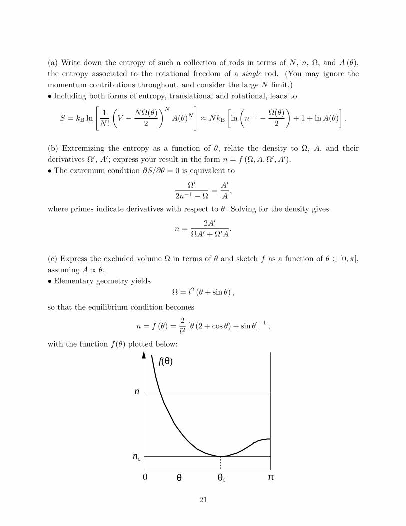
(c) Express the excluded volume Ω in terms of θ and sketch f as a function of θ ∈ [0, π],
assuming A ∝ θ.
• Elementary geometry yields
Ω = l2 (θ + sin θ) ,
so that the equilibrium condition becomes
n = f (θ) = l
2 2
[θ (2 + cos θ) + sin θ]−1 ,
with the function f(θ) plotted below:
n
f(θ)
θc0 θ π
21
nc

(d) Describe the equilibrium state at high densities. Can you identify a phase transition
as the density is decreased? Draw the corresponding critical density nc on your sketch.
What is the critical angle θc at the transition? You don’t need to calculate θc explicitly,
but give an (implicit) relation defining it. What value does θ adopt at n < nc?
• At high densities, θ ≪ 1 and the equilibrium condition reduces to
V N ≈ ;
2θl2
the angle θ is as open as allowed by the close packing. The equilibrium value of θ increases
as the density is decreased, up to its “optimal” value θc at nc, and θ (n < nc) = θc. The
transition occurs at the minimum of f (θ), whence θc satisfies
d [θ (2 + cos θ) + sin θ] = 0,
dθ
i.e.
2 (1 + cos θc) = θc sin θc.
Actually, the above argument tracks the stability of a local maximum in entropy (as density
is varied) which becomes unstable at θc. There is another entropy maximum at θ = π,
corresponding to freely rotating rods, which becomes more advantageous (i.e. the global
equilibrium state) at a density slightly below θc.
********
22

( ) ( )
⟨ ⟩
∑ ¯
∫
∫
8.333: Statistical Mechanics I Fall 2003 Final Exam
1. Helium 4: 4He at low temperatures can be converted from liquid to solid by application
of pressure. An interesting feature of the phase boundary is that the melting pressure is
reduced slightly from its T = 0K value, by approximately 20Nm−2 at its minimum at
T = 0.8K. We will use a simple model of liquid and solid phases of 4He to account for this
feature.
(a) By equating chemical potentials, or by any other technique, prove the Clausius–
Clapeyron equation (dP/dT )melting = (sℓ−ss)/(vℓ−vs), where (vℓ, sℓ) and (vs, ss) are the
volumes and entropies per atom in the liquid and solid phases respectively.
• Clausius-Clapeyron equation can be obtained by equating the chemical potentials at the
phase boundary,
µℓ(T, P ) = µs(T, P ), and µℓ(T + ΔT, P + ΔP ) = µs(T + ΔT, P + ΔP ).
Expanding the second equation, and using the thermodynamic identities
∂µ ∂µ ∂T P
= S, and ∂P T
= −V,
results in ( ) ∂P
= sℓ − ss
. ∂T melting vℓ − vs
(b) The important excitations in liquid 4He at T < 1◦K are phonons of velocity c. Cal
culate the contribution of these modes to the heat capacity per particle CVℓ /N , of the
liquid.
The important excitations in liquid 4He at T < 1◦K are phonons of velocity c. The • corresponding dispersion relation is ε(k) = hck. From the average number of phonons in
mode ~k, given by k) = [exp(β¯ , we obtain the net excitation energy as n(~ hck) − 1]−1
hckEphonons =
exp(β¯hck) − 1 �k
4πk2dk hck = V (change variables to x = βhck¯ )×
(2π)3 exp(βhck) − 1
V ( kBT
)4 6 ∫ ∞ x3 π2
( kBT
)4
= ¯ dx = V ¯ ,hc hc 2π2 hc 3! 0 ex − 1 30 hc
where we have used 1 ∞ x3 π4
ζ4 ≡3! 0
dx ex − 1
=90 .
23

(
The corresponding heat capacity is now obtained as
dE 2π2 ( kBT
)3
CV = = V kB ,dT 15 hc ¯
resulting in a heat capacity per particle for the liquid of
Cℓ 2π2 kBT )3
V = kBvℓ . N 15 hc ¯
(c) Calculate the low temperature heat capacity per particle CVs /N , of solid 4He in terms
of longitudinal and transverse sound velocities cL, and cT .
• The elementary excitations of the solid are also phonons, but there are now two trans
verse sound modes of velocity cT , and one longitudinal sound mode of velocity cL. The
contributions of these modes are additive, each similar inform to the liquid result calculated
above, resulting in the final expression for solid heat capacity of
CVs 2π2
( kBT
)3 ( 2 1
)
= kBvs + . N 15 h c3 c3
× T L
(d) Using the above results calculate the entropy difference (sℓ − ss), assuming a single
sound velocity c ≈ cL ≈ cT , and approximately equal volumes per particle vℓ ≈ vs ≈ v.
Which phase (solid or liquid) has the higher entropy?
• The entropies can be calculated from the heat capacities as
∫ T ( )3
sℓ(T ) = CV
ℓ (T ′)dT ′ =
2π2
kBvℓ kBT
,T ′ 45 hc ¯0
∫ T ( )3 ( ) CV
s (T ′)dT ′ 2π2 kBT 2 1 ss(T ) = = kBvs 3 + 3 .
T ′ 45 h ×
c c0 T L
Assuming approximately equal sound speeds c ≈ cL ≈ cT ≈ 300ms−1, and specific volumes
vℓ ≈ vs ≈ v = A3, we obtain the entropy difference 46˚
4π2 ( kBT
)3
sℓ − ss ≈ − 45
kBv hc ¯
.
The solid phase has more entropy than the liquid because it has two more phonon excitation
bands.
(e) Assuming a small (temperature independent) volume difference δv = vℓ − vs, calculate
the form of the melting curve. To explain the anomaly described at the beginning, which
phase (solid or liquid) must have the higher density?
24

∑ ∑
∏ ∑
• Using the Clausius-Clapeyron equation, and the above calculation of the entropy differ
ence, we get ( ) ( )3∂P
= sℓ − ss
=4π2
kB v kBT
. ∂T melting vℓ − vs
−45 δv hc
Integrating the above equation gives the melting curve
π2 v ( kBT
)3
Pmelt(T ) = P (0) − kB T. 45 δv hc ¯
To explain the reduction in pressure, we need δv = vℓ − vs > 0, i.e. the solid phase has
the higher density, which is expected.
********
2. Surfactant Condensation: N surfactant molecules are added to the surface of water
over an area A. They are subject to a Hamiltonian
N ∑ p~i
2 1 ∑ H =
2m +
2 V(~ri − ~rj),
i=1 i,j
where ~ri and p~i are two dimensional vectors indicating the position and momentum of
particle i.
(a) Write down the expression for the partition function Z(N, T,A) in terms of integrals
over ~ri and p~i, and perform the integrals over the momenta.
• The partition function is obtained by integrating the Boltzmann weight over phase space,
as
∫∏N N 2
i=1 d2p~id
2~qi piZ(N, T,A) = N !h2N
exp −β 2m
− β V(q~i − ~qj) , i=1 i<j
with β = 1/(kBT ). The integrals over momenta are simple Gaussians, yielding
∫ N
1 1 Z(N, T,A) = d2~qi exp −β V(~qi − ~qj) ,
N ! λ2N i=1 i<j
where as usual λ = h/√
2πmkBT denotes the thermal wavelength.
The inter–particle potential V(~r) is infinite for separations ~r < a, and attractive for
|~r | > a such that ∫ ∞
2πrdrV(r) = −u0.
| |a
(b) Estimate the total non–excluded area available in the positional phase space of the
system of N particles.
• To estimate the joint phase space of particles with excluded areas, add them to the
system one by one. The first one can occupy the whole area A, while the second can
25

∑ ∫
∫
[ ]
∣ ∣
∣
explore only A − 2Ω, where Ω = πa2 . Neglecting three body effects (i.e. in the dilute
limit), the area available to the third particle is (A − 2Ω), and similarly (A − nΩ) for the
n-th particle. Hence the joint excluded volume in this dilute limit is
A(A − Ω)(A − 2Ω) (A − (N − 1)Ω) ≈ (A −NΩ/2)N ,· · ·
where the last approximation is obtained by pairing terms m and (N −m), and ignoring
order of Ω2 contributions to their product.
(c) Estimate the total potential energy of the system, assuming a constant density n = N/A.
Assuming this potential energy for all configurations allowed in the previous part, write
down an approximation for Z. ¯• Assuming a uniform density n = N/A, an average attractive potential energy, U , is
estimated as
U =1 Vattr.(~qi − q~j) =
1 d2~r1d
2~r2n(~r1)n(~r2)Vattr.(~r1 − ~r2)2 2
i,j
n2 N2
≈2 A d2~r Vattr.(~r ) ≡ −
2Au0.
Combining the previous results gives
Z(N, T,A) ≈ 1 1(A −NΩ/2)N exp
βu0N2
. N ! λ2N 2A
(d) The surface tension of water without surfactants is σ0, approximately independent of
temperature. Calculate the surface tension σ(n, T ) in the presence of surfactants.
• Since the work done is changing the surface area is dW = σdA, we have dF = −TdS +
σdA + µdN , where F = −kBT lnZ is the free energy. Hence, the contribution of the
surfactants to the surface tension of the film is
∂ lnZ ∣∣
NkBT u0N2
σs = = + ,− ∂A
−A −NΩ/2 2A2
T,N
which is a two-dimensional variant of the familiar van der Waals equation. Adding the
(constant) contribution in the absence of surfactants gives
∂ lnZ ∣∣
NkBT u0N2
σ(n, T ) = σ0 − ∂A ∣
= −A −NΩ/2
+ 2A2
. T,N
(e) Show that below a certain temperature, Tc, the expression for σ is manifestly incorrect.
What do you think happens at low temperatures?
26

∣
∣
∣ ∣ ∣ ∣ ∣ ∣
∣ ∣ ∣
√
• Thermodynamic stability requires δσδA ≥ 0, i.e. σ must be a monotonically increasing
function of A at any temperature. This is the case at high temperatures where the first
term in the equation for σs dominates, but breaks down at low temperatures when the term
from the attractive interactions becomes significant. The critical temperature is obtained
by the usual conditions of ∂σs/∂A = ∂2σs/∂A2 = 0, i.e. from
∂σs
∣
∣ NkBT u0N2
= = 0 ∂A ∣ (A −NΩ/2)2
− A3
T
∂2σs
∣
∣ 2NkBT 3u0N2
,
∣ = + = 0
∂A2 −
(A −NΩ/2)3 A4 T
The two equations are simultaneously satisfied for Ac = 3NΩ/2, at a temperature
8u0Tc = .
27kBΩ
As in the van der Waals gas, at temperatures below Tc, the surfactants separate into a
high density (liquid) and a low density (gas) phase.
(f) Compute the heat capacities, CA and write down an expression for Cσ without explicit
evaluation, due to thesurfactants.
• The contribution of the surfactants to the energy of the film is given by
∂ lnZ kBT u0N2
Es = = 2N .− ∂β
× 2
− 2A
The first term is due to the kinetic energy of the surfactants, while the second arises from
their (mean-field) attraction. The heat capacities are then calculated as
dQ ∣ ∂E ∣ CA = = = NkB,
dT ∂T A A
and ∣ ∣ ∣
dQ ∣ ∂E ∣ ∂A ∣ = .Cσ =
dT ∣ ∂T ∣ − σ
∂T ∣ σ σ σ
********
3. Dirac Fermions are non-interacting particles of spin 1/2. The one-particle states come
in pairs of positive and negative energies,
2 2E±(~k) = ± m c4 + h2k2c ,
independent of spin.
27

∫
∑
∫
(a) For any fermionic system of chemical potential µ, show that the probability of finding
an occupied state of energy µ + δ is the same as that of finding an unoccupied state of
energy µ − δ. (δ is any constant energy.)
• According to Fermi statistics, the probability of occupation of a state of of energy E is
eβ(µ−E )n
p [n(E)] = , for n = 0, 1. 1 + eβ(µ−E )
For a state of energy µ + δ,
eβδn eβδ 1 p [n(µ + δ)] =
1 + e, = ⇒ p [n(µ + δ) = 1] =
1 + eβδ =
1 + e−βδ .
βδ
Similarly, for a state of energy µ − δ,
e−βδn 1 p [n(µ − δ)] =
1 + e−βδ , = ⇒ p [n(µ − δ) = 0] =
1 + e−βδ = p [n(µ + δ) = 1] ,
i.e. the probability of finding an occupied state of energy µ + δ is the same as that of
finding an unoccupied state of energy µ − δ.
(b) At zero temperature all negative energy Dirac states are occupied and all positive
energy ones are empty, i.e. µ(T = 0) = 0. Using the result in (a) find the chemical
potential at finite temperatures T . • The above result implies that for µ = 0, �n(E)� + �n − E)� is unchanged for an tem
perature; any particle leaving an occupied negative energy state goes to the corresponding
unoccupied positive energy state. Adding up all such energies, we conclude that the total
particle number is unchanged if µ stays at zero. Thus, the particle–hole symmetry enfrces
µ(T ) = 0.
(c) Show that the mean excitation energy of this system at finite temperature satisfies
E(T ) − E(0) = 4V (2
d
π
3~k )3 exp
( β
EE+
+
(
(
~k
~k
)
) )
+ 1 .
• Using the label +(-) for the positive (energy) states, the excitation energy is calculated
as E(T ) −E(0) = [�n+(k)� E+(k) + (1 − �n−(k)�) E−(k)]
k,sz
∑ d3~k E+(~k) = 2 = 4V ( ) .
k
2 �n+(k)� E+(k)(2π)3 exp βE+(~k) + 1
28

∫
∣ ∣
• �
∫
(d) Evaluate the integral in part (c) for massless Dirac particles (i.e. for m = 0).
• For m = 0, E+(k) = hc¯ |k|, and
∞ 4πk2dk hck ¯E(T ) −E(0) = 4V
8π3 eβ¯= (set β¯ x)hck =
hck + 1 0
2V ( kBT
)3 ∫ ∞ x3
= kBT dx π2 ¯ 0 ex + 1 hc
7π2 ( kBT
)3
= V kBT . 60 hc
For the final expression, we have noted that the needed integral is 3!f4−(1), and used the
given value of f4−(1) = 7π4/720.
(e) Calculate the heat capacity, CV , of such massless Dirac particles.
• The heat capacity can now be evaluated as
∂E ∣∣
7π2 ( kBT
)3
CV = = V kB . ∂T V 15 hc ¯
(f) Describe the qualitative dependence of the heat capacity at low temperature if the
particles are massive.
When m = 0, there is an energy gap between occupied and empty states, and we thus
expect an exponentially activated energy, and hence heat capacity. For the low energy
excitations, h2¯ k2
E+(k) ≈ mc 2 + + ,2m
· · ·
and thus
E(T ) −E(0) ≈ 2V mc 2 e−βmc2 4π
√π ∞
dxx2 e−x
π2 λ30
√48
π λV 3
e−βmc22 = mc .
The corresponding heat capacity, to leading order thus behaves as
V ( )2 C(T ) ∝ kB
λ3 βmc2 e−βmc2
.
********
29

∫
8.333: Statistical Mechanics I Fall 2004 Final Exam
1. Neutron star core: Professor Rajagopal’s group has proposed that a new phase of QCD
matter may exist in the core of neutron stars. This phase can be viewed as a condensate
of quarks in which the low energy excitations are approximately
( )2
E(~k)± = ± h2
|~k |2
−M
kF
.
The excitations are fermionic, with a degeneracy of g = 2 from spin.
(a) At zero temperature all negative energy states are occupied and all positive energy
ones are empty, i.e. µ(T = 0) = 0. By relating occupation numbers of states of energies
µ + δ and µ − δ, or otherwise, find the chemical potential at finite temperatures T .
• According to Fermi statistics, the probability of occupation of a state of of energy E is
eβ(µ−E )n
p [n(E)] = , for n = 0, 1. 1 + eβ(µ−E )
For a state of energy µ + δ,
eβδn eβδ 1 p [n(µ + δ)] = , = p [n(µ + δ) = 1] = = .
1 + eβδ ⇒
1 + eβδ 1 + e−βδ
Similarly, for a state of energy µ − δ,
e−βδn 1 p [n(µ − δ)] =
1 + e−βδ , = ⇒ p [n(µ − δ) = 0] =
1 + e−βδ = p [n(µ + δ) = 1] ,
i.e. the probability of finding an occupied state of energy µ + δ is the same as that of
finding an unoccupied state of energy µ − δ. This implies that for µ = 0, �n(E)�+ �n(−E)� is unchanged for an temperature; for every particle leaving an occupied negative energy
state a particle goes to the corresponding unoccupied positive energy state. Adding up all
such energies, we conclude that the total particle number is unchanged if µ stays at zero.
Thus, the particle–hole symmetry enforces µ(T ) = 0.
(b) Assuming a constant density of states near k = kF , i.e. setting d3k ≈ 4πk2 dq with F
q = |~k | − kF , show that the mean excitation energy of this system at finite temperature is
E(T ) −E(0) ≈ 2gV k
πF 2
2
∞ dq
exp (β
EE+
+
(
(
q
q
)
)) + 1 .
0
30
∑
∫
∫ ∫
∫
∫
( )
• Using the label +(-) for the positive (energy) states, the excitation energy is calculated
as E(T ) − E(0) = [�n+(k)� E+(k) + (1 − �n−(k)�) E−(k)]
k,s
∑ d3~k E+(~k) = g = 2gV ( ) .
k
2 �n+(k)� E+(k)(2π)3 exp βE+(~k) + 1
The largest contribution to the integral comes for |~k | ≈ kF . and setting q = (|~k | − kF )
and using d3k ≈ 4πk2 dq, we obtain F
4πk2 ∞ E+(q) k2 ∞ E+(q)E(T )−E(0) ≈ 2gV
8π3 F 2 dq
exp (βE+(q)) + 1 = 2gV
πF 2
dq exp (βE+(q)) + 1
. 0 0
(c) Give a closed form answer for the excitation energy by evaluating the above integral.
For E+(q) = h2 q2/(2M), we have •
E(T ) −E(0) = 2gV kF
2 ∞ dq
h2 q2/2M = (set βh2 q 2/2M = x)
π2 eβh2q2/2M + 1 0
gV k2 (
2MkBT )1/2 ∞ x1/2
= F kBT dx π2 h2
0 ex + 1
gV kF 2
( 2MkBT
)1/2 √π (
1 ) (
1 ) ζ3/2 V kF
2
= π2
kBT h2 2
1 − √2
ζ3/2 = 1 − √2 π λ
kBT.
For the final expression, we have used the value of f−(1), and introduced the thermal m
wavelength λ = h/√
2πMkBT .
(d) Calculate the heat capacity, CV , of this system, and comment on its behavior at low
temperature.
Since E ∝ T 3/2 ,•
CV =∂E ∣
∣
∣ =
3 E =
3ζ3/2 1 V kF 2 √
T . ∂T ∣ V 2 T 2π
1 − √2 λ
kB ∝
This is similar to the behavior of a one dimensional system of bosons (since the density
of states is constant in q as in d = 1). Of course, for any fermionic system the density of
states close to the Fermi surface has this character. The difference with the usual Fermi
systems is the quadratic nature of the excitations above the Fermi surface.
********
2. Critical point behavior: The pressure P of a gas is related to its density n = N/V , and
temperature T by the truncated expansion
cb 2 3P = kBTn − n + n ,2 6
31

∣ ∣
∣ ∣ ∣ ∣ ∣
( )
where b and c are assumed to be positive temperature independent constants.
(a) Locate the critical temperature Tc below which this equation must be invalid, and
the corresponding density nc and pressure Pc of the critical point. Hence find the ratio
kBTcnc/Pc.
• Mechanical stability of the gas requires that any spontaneous change in volume should be
opposed by a compensating change in pressure. This corresponds to δPδV < 0, and since
δn = −(N/V 2)δV , any equation of state must have a pressure that is an increasing func
tion of density. The transition point between pressure isotherms that are monotonically
increasing functions of n, and those that are not (hence manifestly incorrect) is obtained
by the usual conditions of dP/dn = 0 and d2P/dn2 = 0. Starting from the cubic equation
of state, we thus obtain dP c
=kBTc − bnc + n 2 = 0 dn 2 c
d2P.
dn2 = − b + cnc = 0
From the second equation we obtain nc = b/c, which substituted in the first equation
gives kBTc = b2/(2c). From the equation of state we then find Pc = b3/(6c2), and the
dimensionless ratio of kBTcnc
= 3. Pc
1 ∂V (b) Calculate the isothermal compressibility κT = V ∂P T, and sketch its behavior as a −
function of T for n = nc.
• Using V = N/n, we get
κT (n) =1 ∂V ∣
=1 ∂P
∣
∣
−1
= [ n ( kBT − bn + cn 2/2
)]−1 .−
V ∂P T n ∂n T
For n = nc, κT (nc) ∝ (T − Tc)−1, and diverges at Tc.
(c) On the critical isotherm give an expression for (P − Pc) as a function of (n − nc).
• Using the coordinates of the critical point computed above, we find
b3 b2 b c P − Pc = −
6c2 +
2cn −
2 n 2 +
6 n 3
c b b2 b3 =
6 n 3 − 3
cn 2 + 3
c2n −
c3
c 3 = (n − nc) .
6
(d) The instability in the isotherms for T < Tc is avoided by phase separation into a liquid
of density n+ and gas of density n−. For temperatures close to Tc, these densities behave
32
( )
( ) ( )
( )
√
∫
∑ ∑ ∑ ∑
as n± ≈ nc (1 ± δ). Using a Maxwell construction, or otherwise, find an implicit equation
for δ(T ), and indicate its behavior for (Tc − T ) 0. (Hint: Along an isotherm, variations →of chemical potential obey dµ = dP/n.)
• According to the Gibbs–Duhem relation, the variations of the intensive variables are
related by SdT − V dP + Ndµ = 0, and thus along an isotherm (dT = 0) dµ = dP/n =
∂P/∂n Tdn/n. Since the liquid and gas states are in coexistence they should have the |same chemical potential. Integrating the above expression for dµ from n to n+ leads to − the so-called Maxwell construction, which reads
∫ n+ ∫ nc(1+δ)
0 = µ(n+) − µ(n ) = dP
= dn kBT − bn + cn2/2
.−n−
n nc(1−δ) n
Performing the integrals gives the equation
0 = kBT ln 1 + δ − bnc(2δ) +
cnc
2 [ (1 + δ)2 − (1 − δ)2
] = kBT ln
1 + δ − 2kBTcδ, 1 − δ 4 1 − δ
where for the find expression, we have used nc = b/c and kBTc = b2/(2c). The implicit
equation for δ is thus
δ =2
T
Tc ln
1 + δ ≈T
T
c
( δ − δ3 + · · ·
) .
1 − δ
The leading behavior as (Tc − T ) 0 is obtained by keeping up to the cubic term, and →given by
Tc .δ ≈ 1 −
T
********
3. Relativistic Bose gas in d dimensions: Consider a gas of non-interacting (spinless)
bosons with energy ǫ = c |p~ |, contained in a box of “volume” V = Ld in d dimensions.
(a) Calculate the grand potential G = −kBT lnQ, and the density n = N/V , at a chemical
potential µ. Express your answers in terms of d and f+ (z), where z = eβµ, and m
1 ∞ xm−1
f+ (z) = dx. m (m − 1)! 0 z−1ex − 1
(Hint: Use integration by parts on the expression for lnQ.)
We have •ni =N ( )
i∞Q Nβµ −β niǫi = e exp
N=0 {ni} i , ∏∑ ∏ 1β(µ−ǫi)ni= e =
i {ni} i 1 − eβ(µ−ǫi)
33

[ ]
∫
( )
∣
whence lnQ = ∑
ln (
eβ(µ−ǫi)) . Replacing the summation
∑ with a d dimensional
∫ − i 1 −
∫ i
integration ∞V ddk/ (2π)
d = V Sd/ (2π)
d ∞kd−1dk, where Sd = 2πd/2/ (d/2 − 1)!,
0 0
leads to V Sd
∞ (
hck)
lnQ = − kd−1dk ln 1 − ze−β¯ .d
(2π) 0
The change of variable x = βhck results in
lnQ = V Sd
( kBT
)d ∫ ∞ x d−1dx ln ze−x .
¯−
(2π)d hc 0
1 −
Finally, integration by parts yields
V Sd 1 ( kBT
)d ∫ ∞ ze−x Sd
( kBT
)d ∫ ∞ xd
lnQ =(2π)
d d hc 0
x ddx 1 − ze−x
= Vd hc 0
dx z−1ex − 1
,
leading to ( )d
Sd kBT G = −kBT lnQ = −Vd hc
kBTd!fd++1 (z) ,
which can be somewhat simplified to
V πd/2d! G = −kBTλc
d (d/2)! fd
++1 (z) ,
where λc ≡ hc/(kBT ). The average number of particles is calculated as
N = ∂G
= −βz ∂G = λ
V d
πd/2d! fd
+ (z) ,−∂µ ∂z c (d/2)!
where we have used z∂fd+1(z)/∂z = fd(z). Dividing by volume, the density is obtained as
1 πd/2d! n =
λd (d/2)! fd
+ (z) . c
(b) Calculate the gas pressure P , its energy E, and compare the ratio E/(PV ) to the
classical value.
• We have PV = −G, while
∂ lnQ ∣ lnQE = ∣ = +d =−
∂β ∣ β −dG.
z
Thus E/(PV ) = d, identical to the classical value for a relativistic gas.
34

∣ ∣
(c) Find the critical temperature, Tc (n), for Bose-Einstein condensation, indicating the
dimensions where there is a transition.
• The critical temperature Tc (n) is given by
1 πd/2d! 1 πd/2d! n = fd
+ (z = 1) = ζd. λd
c (d/2)! λdc (d/2)!
This leads to hc ( n(d/2)!
)1/d
Tc = . kB πd/2d!ζd
However, ζd is finite only for d > 1, and thus a transition exists for all d > 1.
(d) What is the temperature dependence of the heat capacity C (T ) for T < Tc (n)?
At T < Tc, z = 1 and E = −dG ∝ T d+1, resulting in •
∂E ∣ E V πd/2d! C (T ) =
∂T ∣ = (d + 1)
T = −d(d + 1)
T G
= d(d + 1) λdkB
(d/2)! ζd+1 ∝ T d .
z=1 c
(e) Evaluate the dimensionless heat capacity C(T )/(NkB) at the critical temperature
T = Tc, and compare its value to the classical (high temperature) limit.
• We can divide the above formula of C(T ≤ Tc), and the one obtained earlier for N(T ≥ Tc), and evaluate the result at T = Tc (z = 1) to obtain
C(Tc) d(d + 1)ζd+1 = .
NkB ζd
In the absence of quantum effects, the heat capacity of a relativistic gas is C/(NkB) = d;
this is the limiting value for the quantum gas at infinite temperature.
********
35

∣ ∣ ∣ ∣
∫
8.333: Statistical Mechanics I Fall 2005 Final Exam
1. Graphene is a single sheet of carbon atoms bonded into a two dimensional hexagonal
lattice. It can be obtained by exfoliation (repeated peeling) of graphite. The band struc
ture of graphene is such that the single particles excitations behave as relativistic Dirac
fermions, with a spectrum that at low energies can be approximated by
E±(~k) = ±hv ∣ ~k∣ .
There is spin degeneracy of g = 2, and v 106ms−1 . Recent experiments on unusual ≈transport properties of graphene were reported in Nature 438, 197 (2005). In this problem,
you shall calculate the heat capacity of this material.
(a) If at zero temperature all negative energy states are occupied and all positive energy
ones are empty, find the chemical potential µ(T ). • According to Fermi statistics, the probability of occupation of a state of of energy E is
eβ(µ−E )n
p [n(E)] = , for n = 0, 1. 1 + eβ(µ−E )
For a state of energy µ + δ,
eβδn eβδ 1 p [n(µ + δ)] =
1 + eβδ , = ⇒ p [n(µ + δ) = 1] =
eβδ =
e−βδ .
1 + 1 +
Similarly, for a state of energy µ − δ,
e−βδn 1 p [n(µ − δ)] =
1 + e−βδ , = ⇒ p [n(µ − δ) = 0] =
1 + e−βδ = p [n(µ + δ) = 1] ,
i.e. the probability of finding an occupied state of energy µ + δ is the same as that of
finding an unoccupied state of energy µ − δ.
At zero temperature all negative energy Dirac states are occupied and all positive
energy ones are empty, i.e. µ(T = 0) = 0. The above result implies that for µ = 0,
�n(E)� + �n − E)� is unchanged for all temperatures; any particle leaving an occupied
negative energy state goes to the corresponding unoccupied positive energy state. Adding
up all such energies, we conclude that the total particle number is unchanged if µ stays at
zero. Thus, the particle–hole symmetry enforces µ(T ) = 0.
(b) Show that the mean excitation energy of this system at finite temperature satisfies
E(T ) − E(0) = 4Ad2~k
( β
EE+
+
(
(
~k
~
) ) .
(2π)2 exp k) + 1
36

∑
∫
∫
∫
∣
• Using the label +(-) for the positive (energy) states, the excitation energy is calculated
as
E(T ) − E(0) = [�n+(k)� E+(k) + (1 − �n−(k)�) E−(k)] k,sz
∑ d2~k k) = 2 = 4A ( ) .
k
2 �n+(k)� E+(k)(2π)2 exp β
EE+
+
(
(
~
~k) + 1
(c) Give a closed form answer for the excitation energy by evaluating the above integral.
• For E+(k) = hv|k|, and
∞ 2πkdk hvk E(T ) − E(0) = 4A
4π2 eβ¯= (set β¯ x)hck =
hvk + 1 0
2A ( kBT
)2 ∫ ∞ x2
= kBT dx π ¯ 0 ex + 1 hv
( )23ζ3 kBT
= AkBT . π hv
For the final expression, we have noted that the needed integral is 2!f3−(1), and used
f3−(1) = 3ζ3/4.
E(T ) − E(0) = A (2
d
π
2~k )2 exp
( β
EE+
+
(
(
~k
~k
)
) ) − 1
.
(d) Calculate the heat capacity, CV , of such massless Dirac particles.
• The heat capacity can now be evaluated as
∣ ( )2
∂E ∣ 9ζ3 kBT CV = = AkB .
∂T V ¯∣ π hv
(e) Explain qualitatively the contribution of phonons (lattice vibrations) to the heat capac
ity of graphene. The typical sound velocity in graphite is of the order of 2×10⁴ms−1 . Is the
low temperature heat capacity of graphene controlled by phonon or electron contributions?
• The single particle excitations for phonons also have a linear spectrum, with Ep = hvp|k|and correspond to µ = 0. Thus qualitatively they give the same type of contribution to
energy and heat capacity. The difference is only in numerical pre-factors. The precise
37
∫
∑ ∑
∑ ∑
contribution from a single phonon branch is given by
∞ 2πkdk hvpk Ep(T ) − Ep(0) = A
0 4π2 eβ¯ k − 1 = (set β¯ x)hck =
hvp
A ( kBT
)2 ∫ ∞ x2
= kBT dx 2π ¯ 0 ex − 1hvp
( )2 ( )2ζ3 kBT 3ζ3 kBT
= AkBT , CV,p = AkB . π ¯ π hvphvp ¯
We see that the ratio of electron to phonon heat capacities is proportional to (vp/v)2 . Since
the speed of Dirac fermions is considerably larger than that of phonons, their contribution
to heat capacity of graphene is negligible.
********
2. Quantum Coulomb gas: Consider a quantum system of N positive, and N negative
charged relativistic particles in box of volume V = L3 . The Hamiltonian is
2N 2N
= c p~i + eiej
,Hi=1
| |i<j
|~ri − ~rj |
where ei = +e0 for i = 1, N , and ei = −e0 for i = N + 1, 2N , denote the charges of · · · · · · the particles; {~ri} and {p~i} their coordinates and momenta respectively. While this is too
complicated a system to solve, we can nonetheless obtain some exact results.
(a) Write down the Schrodinger equation for the eigenvalues εn(L), and (in coordinate
space) eigenfunctions Ψn({~ri}). State the constraints imposed on Ψn({~ri}) if the particles
are bosons or fermions?
• In the coordinate representation ~pi is replaced by −ih∇i, leading to the Schrodinger
equation
2N 2N eiej
c| − ih∇i | + ~ri − ~rj
Ψn({~ri}) = εn(L)Ψn({~ri}). i=1 i<j
| |
There are N identical particles of charge +e0, and N identical particles of charge −e0. We can examine the effect of permutation operators P+ and P on these two sets. The − symmetry constraints can be written compactly as
P+ P−P+P−Ψn({~ri}) = η+ · η− Ψn({~ri}),
where η = +1 for bosons, η = −1 for fermions, and (−1)P denotes the parity of the
permutation. Note that there is no constraint associated with exchange of particles with
opposite charge.
38

( ) ( )
( )
(b) By a change of scale ~ri ′ = ~ri/L, show that the eigenvalues satisfy a scaling relation
εn(L) = εn(1)/L.
• After the change of scale ~ri ′ = ~ri/L (and corresponding change in the derivative
∇i ′ = L∇i), the above Schrodinger equation becomes
2N ∣ ∣ 2N ({ }) ({ })
∑ c ∣∣
∣
−ih∇i ′ ∣
∣ + ∑ eiej
Ψn ~ri
′ = εn(L)Ψn
~ri ′
. i=1
L ∣ i<j
L |~ri ′ − ~rj ′| L L
The coordinates in the above equation are confined to a box of unit size. We can regard it
as the Schrodinger equation in such a box, with wave-functions Ψ′ n({~ri}) = Ψn ({~ri ′/L}).
The corresponding eigenvalues are εn(1) = Lεn(L) (obtained after multiplying both sides
of the above equation by L We thus obtain the scaling relation
εn(1) εn(L) = .
L
(c) Using the formal expression for the partition function Z(N, V, T ), in terms of the
eigenvalues {εn(L)}, show that Z does not depend on T and V separately, but only on a
specific scaling combination of them.
• The formal expression for the partition function is
Z(N, V, T ) = tr e−βH = ∑
exp − εkn
B
(L
T )
n
∑ εn(1) = exp ,−
kBTL n
where we have used the scaling form of the energy levels. Clearly, in the above sum T and
L always occur in the combination TL. Since V = L3, the appropriate scaling variable is
V T 3, and
Z(N, V, T ) = Z(N, V T 3).
(d) Relate the energy E, and pressure P of the gas to variations of the partition function.
Prove the exact result E = 3PV . • The average energy in the canonical ensemble is given by
E = ∂ lnZ
= kBT 2∂ lnZ
= kBT 2(3V T 2) ∂ lnZ
= 3kBV T 4 ∂ lnZ
.− ∂β ∂T ∂(V T 3) ∂(V T 3)
The free energy is F = −kBT lnZ, and its variations are dF = −SdT − PdV + µdN .
Hence the gas pressure is given by
P = ∂F
= kBT∂ lnZ
= kBT 4 ∂ lnZ
.−∂V ∂V ∂(V T 3)
39

∑
∑ ∑
{ } { }
• { }
{ } [ ]
The ratio of the above expressions gives the exact identity E = 3PV .
(e) The Coulomb interaction between charges in in d-dimensional space falls off with sepa
ration as eiej/ |~ri − ~rj | d−2 . (In d = 2 there is a logarithmic interaction.) In what dimension
d can you construct an exact relation between E and P for non-relativistic particles (ki
netic energy i p~i2/2m)? What is the corresponding exact relation between energy and
pressure?
• The above exact result is a consequence of the simple scaling law relating the energy
eigenvalues εn(L) to the system size. We could obtain the scaling form in part (b) since
the kinetic and potential energies scaled in the same way. The kinetic energy for non
relativistic particles i p~i2/2m = i h
2 i2/2m, scales as 1/L2 under the change of scale − ∇∑2N d−2
~ri ′ = ~ri/L, while the interaction energy i<j eiej/ |~ri − ~rj | in d space dimensions
scales as 1/Ld−2 . The two forms will scale the same way in d = 4 dimensions, leading to
εn(1) εn(L) = .
L2
The partition function now has the scaling form
Z(N, V = L4, T ) = ( N, (TL2)2
) =
( N, V T 2
) .Z Z
Following steps in the previous part, we obtain the exact relationship E = 2PV .
(f) Why are the above ‘exact’ scaling laws not expected to hold in dense (liquid or solid)
Coulomb mixtures?
• The scaling results were obtained based on the assumption of the existence of a single
scaling length L, relevant to the statistical mechanics of the problem. This is a good
approximation in a gas phase. In a dense (liquid or solid) phase, the short-range repulsion
between particles is expected to be important, and the particle size a is another relevant
length scale which will enter in the solution to the Schrodinger equation, and invalidate
the scaling results.
********
3. Non-interacting Fermions: Consider a grand canonical ensemble of non-interacting
fermions with chemical potential µ. The one–particle states are labelled by a wavevector ~k, and have energies E(~k).
(a) What is the joint probability P ( n�k ), of finding a set of occupation numbers n�k ,
of the one–particle states?
In the grand canonical ensemble with chemical potential µ, the joint probability of
finding a set of occupation numbers n� , for one–particle states of energies E(~k) is given k
by the Fermi distribution
∏ exp k))n�k P ( n�k
) = β([ µ − E(~
] , where n�k = 0 or 1, for each ~k.
�k 1 + exp β(µ − E(~k))
40

{ } ⟨ ⟩
⟨ ⟩ [ ]
{ } ⟨ ⟩∏[ ] ⟨ ⟩
∑
∑ ⟨ ⟩ ⟨ ⟩ ⟨ ⟩ ⟨ ⟩
(b) Express your answer to part (a) in terms of the average occupation numbers n�k . − • The average occupation numbers are given by
exp β(µ − E(~k)) n� = [ ] ,
k − 1 + exp β(µ − E(~k))
from which we obtain ⟨ ⟩
exp [ β(µ − E(~k))
] =
1 − n⟨ �k
n�k
−⟩ . −
This enables us to write the joint probability as
~k )1−n
P ( n�k ) = n�k − 1 − n�k − . �k
(c) A random variable has a set of ℓ discrete outcomes with probabilities pn, where n =
1, 2, , ℓ. What is the entropy of this probability distribution? What is the maximum · · · possible entropy?
• A random variable has a set of ℓ discrete outcomes with probabilities pn. The entropy
of this probability distribution is calculated from
ℓ
S = −kB pn ln pn . n=1
The maximum entropy is obtained if all probabilities are equal, pn = 1/ℓ, and given by
Smax = kB ln ℓ.
(d) Calculate the entropy of the probability distribution for fermion occupation numbers
in part (b), and comment on its zero temperature limit.
• Since the occupation numbers of different one-particle states are independent, the cor
responding entropies are additive, and given by
~k ( )n (
[ ( ) ( )] S = −kB n�k − ln n�k − + 1 − n�k − ln 1 − n�k − .
�k
In the zero temperature limit all occupation numbers are either 0 or 1. In either case the
contribution to entropy is zero, and the fermi system at T = 0 has zero entropy.
(e) Calculate the variance of the total number of particles ⟨ N2⟩
c, and comment on its zero
temperature behavior.
41

∑
∑ ∑ ∑ ( )
⟨ ⟩
⟨ ⟩
⟨ ⟩
• The total number of particles is given by N = �k n�k. Since the occupation numbers
are independent
⟨ ⟩ ⟨ ⟩ ( ) ⟨ ⟩
2 2 ⟨ ⟩2 ⟨ ⟩ ⟨ ⟩
N2c
= n�k c = n�k −
− n�k = n�k − 1 − n�k
,− −�k �k �k
since n�2 =
⟨ n�k
⟩ . Again, since at T = 0,
⟨ n�k
⟩ = 0 or 1, the variance
⟨ N2⟩
ck − − − vanishes.
(f) The number fluctuations of a gas is related to its compressibility κT , and number
density n = N/V , by
N2 = NnkBTκT . c
Give a numerical estimate of the compressibility of the fermi gas in a metal at T = 0 in
units of ˚ .A3eV −1
To obtain the compressibility from N2 = NnkBTκT , we need to examine the behavior c
• at small but finite temperatures. At small but finite T , a small fraction of states around the
fermi energy have occupation numbers around 1/2. The number of such states is roughly
NkBT/εF , and hence we can estimate the variance as
⟨ ⟩ 1 NkBT N2
c = NnkBTκT ≈
4 ×
εF .
The compressibility is then approximates as
1 ,κT ≈
4nεF
where n = N/V is the density. For electrons in a typical metal n ≈ 1029 ≈ 0.1˚m−3 A3, and
εF ≈ 5eV ≈ 5 × 10⁴ ◦K, resulting in
A3eV −1 .κT ≈ 0.5˚
********
42

( ) ( )
( )
⟨ ⟩
∑ ¯
∫
∫
8.333: Statistical Mechanics I Fall 2006 Final Exam
1. Freezing of He4: At low temperatures He4 can be converted from liquid to solid by
application of pressure. An interesting feature of the phase boundary is that the melting
pressure is reduced slightly from its T = 0K value, by approximately 20Nm−2 at its
minimum at T = 0.8K. We will use a simple model of liquid and solid phases of 4He to
account for this feature.
(a) By equating chemical potentials, or by any other technique, prove the Clausius–
Clapeyron equation (dP/dT )melting = (sℓ−ss)/(vℓ−vs), where (vℓ, sℓ) and (vs, ss) are the
volumes and entropies per atom in the liquid and solid phases respectively.
• Clausius-Clapeyron equation can be obtained by equating the chemical potentials at the
phase boundary,
µℓ(T, P ) = µs(T, P ), and µℓ(T + ΔT, P + ΔP ) = µs(T + ΔT, P + ΔP ).
Expanding the second equation, and using the thermodynamic identities
∂µ ∂µ ∂T P
= S, and ∂P T
= −V,
results in ∂P
= sℓ − ss
. ∂T melting vℓ − vs
(b) The important excitations in liquid 4He at T < 1K are phonons of velocity c. Calculate
the contribution of these modes to the heat capacity per particle CVℓ /N , of the liquid.
The dominant excitations in liquid 4He at T < 1K are phonons of velocity c. The • corresponding dispersion relation is ε(k) = hck. From the average number of phonons in
mode ~k, given by k) = [exp(β¯ , we obtain the net excitation energy as n(~ hck) − 1]−1
hckEphonons =
exp(β¯hck) − 1 �k
4πk2dk hck = V (change variables to x = βhck¯ )×
(2π)3 exp(βhck¯ ) − 1
V ( kBT
)4 6 ∫ ∞ x3 π2
( kBT
)4
= ¯ dx = V ¯ ,hc hc 2π2 ¯ 3! 0 − 1 30 hc ¯hc ex
where we have used 1 ∞ x3 π4
ζ4 ≡3! 0
dx ex − 1
=90 .
43
(
The corresponding heat capacity is now obtained as
dE 2π2 ( kBT
)3
CV = = V kB ,dT 15 hc ¯
resulting in a heat capacity per particle for the liquid of
Cℓ 2π2 kBT )3
V = kBvℓ . N 15 hc ¯
(c) Calculate the low temperature heat capacity per particle CVs /N , of solid 4He in terms
of longitudinal and transverse sound velocities cL, and cT .
• The elementary excitations of the solid are also phonons, but there are now two trans
verse sound modes of velocity cT , and one longitudinal sound mode of velocity cL. The
contributions of these modes are additive, each similar inform to the liquid result calculated
above, resulting in the final expression for solid heat capacity of
CVs 2π2
( kBT
)3 ( 2 1
)
= kBvs + . N 15 h c3 c3
× T L
(d) Using the above results calculate the entropy difference (sℓ − ss), assuming a single
sound velocity c ≈ cL ≈ cT , and approximately equal volumes per particle vℓ ≈ vs ≈ v.
Which phase (solid or liquid) has the higher entropy?
• The entropies can be calculated from the heat capacities as
∫ T ( )3
sℓ(T ) = CV
ℓ (T ′)dT ′ =
2π2
kBvℓ kBT
,T ′ 45 hc ¯0
∫ T ( )3 ( ) CV
s (T ′)dT ′ 2π2 kBT 2 1 ss(T ) = = kBvs 3 + 3 .
T ′ 45 h ×
c c0 T L
Assuming approximately equal sound speeds c ≈ cL ≈ cT ≈ 300ms−1, and specific volumes
vℓ ≈ vs ≈ v = A3, we obtain the entropy difference 46˚
4π2 ( kBT
)3
sℓ − ss ≈ − 45
kBv hc ¯
.
The solid phase has more entropy than the liquid because it has two more phonon excitation
bands.
(e) Assuming a small (temperature independent) volume difference δv = vℓ − vs, calculate
the form of the melting curve. To explain the anomaly described at the beginning, which
phase (solid or liquid) must have the higher density?
44
• Using the Clausius-Clapeyron equation, and the above calculation of the entropy differ
ence, we get ( ) ( )3∂P sℓ − ss 4π2 v kBT ∂T melting
= vℓ − vs
= −45
kB ¯
. δv hc
Integrating the above equation gives the melting curve
π2 v ( kBT
)3
Pmelt(T ) = P (0) − kB T. 45 δv hc ¯
To explain the reduction in pressure, we need δv = vℓ − vs > 0, i.e. the solid phase has
the higher density, which is normal.
********
2. Squeezed chain: A rubber band is modeled as a single chain of N massless links of fixed
length a. The chain is placed inside a narrow tube that restricts each link to point parallel
or anti-parallel to the tube.
(a) Ignoring any interactions amongst the links, give the number of configurations of the
chain, Ω(L,N), where L is the end–to–end length of the chain.
• A typical configuration will have N+ steps in one direction, and N− steps in the opposite
direction, such that
L = (N+ −N−)a, and N = N+ + N−,
or equivalently N ± L/a
N = .± 2
The number of configurations is given by the binomial formula
N ! N ! Ω(L,N) = = .
N+!N−! [(N + L/a)/2]![(N − L/a)/2]!
(b) Use Stirling’s approximation to express the result for entropy as a function of N and
x = L/(Na).
• Using Stirling’s approximation
S kB
= ln Ω ≈ N lnN −N+ lnN+ −N− lnN−
N = N ln 2 − [(1 + x) ln(1 + x) + (1 − x) ln(1 − x)] .
2
45

( )
√ ( )
The tube is now uniformly squeezed such that stretched configurations are energet
ically favored. For this problem, assume a simplified form of this energy that depends
inversely on the local link density, such that the energy of a uniformly stretched state is
σ L σa2
E(L,N) = L = Nx2 .−2
×N
− 2
(Use this formula for energy for all states of given L and N in the remainder of this
problem.)
(c) Calculate the free energy F (T, L,N), and the force J(T, L,N) acting on the end points
of the chain. (The work done on expanding the chain is dW JdL.) ¯ =
• The free energy is
σ L2 kBT F = E−TS = −
2 N +
2[(N + L/a) ln(N + L/a) + (N − L/a) ln(N − L/a) −N ln 2 − 2N lnN ] .
The force conjugate to L is obtained as
∂F L kBT Na + L kBT 1 + x J =
∂L = −σ
N +
2a ln Na − L
= −σax +2a
ln 1 − x
.
(d) Sketch the isotherms J(x, T ) at high and low temperatures, and identify the tempera
ture Tc when the behavior changes.
• The curves J(x) start linearly at x = 0 with a slope (kBT/a − σa), and go to (plus)
infinity as x 1. The slope changes sign at Tc = (σa2)/kB, with the curves for T < Tc→being non-monotonic in x.
(e) What is the condition for stability of the chain? What portion of the above isotherms
are inherently unstable.
• The condition for stability
δJδL ≥ 0,
implies that the slope of the isotherm J(x) must be positive. The portion of the isotherms
below the minimum for T < Tc violate this condition, and are inherently unstable.
(f) Using the form for J obtained in part (c), find an expression for the unforced (J = 0)
chain length that is valid as T approaches Tc from below.
• As T → T −, x ∝ L goes to zero. Expanding the logarithms in the expression for c
J(x) = 0, we find
0 = −σa +2kBT
x +2kBT
x 3 + O(x 5). a 3a
The solution to this equation is
x2 Tc Tc = 1 − , L ≈ Na 3 1 − .
3 T T
46

∣ ∣
********
3. Graphene bilayer: The layers of graphite can be peeled apart through different exfo
liation processes. Many such processes generate single sheets of carbon atoms, as well as
bilayers in which the two sheets are weakly coupled. The hexagonal lattice of the single
layer graphene, leads to a band structure that at low energies can be approximated by 1 layer (~k) = (ak), as in relativistic Dirac fermions. (Here k =
∣
∣ ~k∣
∣, a is a lattice spac-E± ±t�
ing, and t is a typical in-plane hopping energy.) A weak hopping energy t between the � ⊥ two sheets of the bilayer modifies the low energy excitations drastically, to
t2 bilayer (~k) =
� (ka)2 ,E± ±
2t⊥
i.e. resembling massive Dirac fermions. In addition to the spin degeneracy, there are two
branches of such excitations per unit cell, for an overall degeneracy of g = 4.
(a) For the undoped material with one electron per site, at zero temperature all negative
energy states are occupied and all positive energy ones are empty. Find the chemical
potential µ(T ). • According to Fermi statistics, the probability of occupation of a state of of energy E is
eβ(µ−E )n
p [n(E)] = , for n = 0, 1. 1 + eβ(µ−E )
For a state of energy µ + δ,
eβδn eβδ 1 p [n(µ + δ)] =
1 + eβδ , = ⇒ p [n(µ + δ) = 1] =
1 + eβδ =
1 + e−βδ .
Similarly, for a state of energy µ − δ,
e−βδn 1 p [n(µ − δ)] =
1 + e−βδ , = ⇒ p [n(µ − δ) = 0] =
1 + e−βδ = p [n(µ + δ) = 1] ,
i.e. the probability of finding an occupied state of energy µ + δ is the same as that of
finding an unoccupied state of energy µ − δ.
At zero temperature all negative energy Dirac states are occupied and all positive
energy ones are empty, i.e. µ(T = 0) = 0. The above result implies that for µ = 0,
�n(E)� + �n − E)� is unchanged for all temperatures; any particle leaving an occupied
negative energy state goes to the corresponding unoccupied positive energy state. Adding
up all such energies, we conclude that the total particle number is unchanged if µ stays at
zero. Thus, the particle–hole symmetry enforces µ(T ) = 0.
47

∫
∑
∫
∫
∫
�
∣ ( )
�
(b) Show that the mean excitation energy of this system at finite temperature satisfies
E(T ) − E(0) = 2gA (2
d
π
2~k )2 exp
( β
EE+
+
(
(
~k
~k
)
) )
+ 1 .
• Using the label +(-) for the positive (energy) states, the excitation energy is calculated
as
E(T ) − E(0) = [�n+(k)� E+(k) + (1 − �n−(k)�) E−(k)] k,sz,α
∑ d2~k E+(~k) = g = 2gA ( ) .
k
2 �n+(k)� E+(k)(2π)2 exp βE+(~k) + 1
(c) Give a closed form answer for the excitation energy of the bilayer by evaluating the
above integral.
• Let E+(k) = αk2, with α = (t�a)2/(2t⊥), to get
E(T ) − E(0) = 2gA ∞ 2πkdk αk2
= (set βαk2 = x) 0 4π2 eβαk2 + 1
gA ( kBT
) ∞ x = kBT dx
2π α 0 ex + 1 ( ) ( )2
gπ kBT π A kBT = AkBT = t
24 α 3 a2 t⊥.
For the final expression, we have noted that the needed integral is f2−(1), and used f2
−(1) =
ζ2/2 = π2/12.
(d) Calculate the heat capacity, CA, of such massive Dirac particles.
• The heat capacity can now be evaluated as
∂E ∣ 2π A kBTtCA =
∂T ∣∣ A
=3 a2
kB t2
⊥ .
(e) A sample contains an equal proportion of single and bilayers. Estimate (in terms of the
hopping energies) the temperature below which the electronic heat capacity is dominated
by the bilayers.
• As stated earlier, the monolayer excitations for phonons have a linear spectrum, with
E1 layer = ±t�(ka). Their contribution to energy and heat capacity can be calculated as
48

∫
� �
before. Including the various prefactors (which are not required for the solution), we have
E1 layer(T ) = 2gA ∞ 2πkdk t�ak
= (set βt ak = x) 0 4π2 eβt‖ak + 1
�
2gA ( kBT
)2 ∫ ∞ x= kBT dx
π t�a 0 ex + 1 ( )2 ( )2
∝a
A kBT
kB
t
T , C1 layer ∝
a
A kB
kB
t
T .
2 A 2
The bilayer heat capacity, which is proportional to T is more important at lower temper
atures. By comparing the two expressions, it is apparent that the electronic heat capacity
per particle is larger in the bilayer for temperatures smaller than T ∗ ≈ t⊥/kB.
********
49

MIT OpenCourseWarehttp://ocw.mit.edu
8.333 Statistical Mechanics I: Statistical Mechanics of ParticlesFall 2013
For information about citing these materials or our Terms of Use, visit: http://ocw.mit.edu/terms.