statistical analysis of windspeed data

Energy Conversion and Management 46 (2005) 515–532www.elsevier.com/locate/enconman

A statistical analysis of wind speed data used in installationof wind energy conversion systems

E. Kavak Akpinar a,*, S. Akpinar b

a Mechanical Engineering Department, Firat University, 23279 Elazig, Turkeyb Physics Department, Firat University, 23279 Elazig, Turkey

Received 20 March 2004; accepted 25 May 2004

Available online 3 July 2004

Abstract

Wind speed is the most important parameter in the design and study of wind energy conversion systems.

In this study, statistical methods were used to analyze the wind speed data of Keban-Elazig in the east

region of Turkey. Measured hourly time series of wind speed data were obtained from the State Meteo-

rological Station in Keban-Elazig over a five year period from 1998 to 2002. The probability density dis-

tributions are derived from the time series data and the distributional parameters are identified. Two

probability density functions are fitted to the measured probability distributions on a yearly basis.

� 2004 Elsevier Ltd. All rights reserved.

Keywords: Weibull distributions; Rayleigh distributions; Weibull parameter; Wind speed data; Wind energy

1. Introduction

Effective utilization of wind energy entails a detailed knowledge of the wind characteristics atthe particular location. The distribution of wind speeds is important for the design of windfarms, power generators and agricultural applications like irrigation. It is not an easy task tochoose a site where wind energy conversion systems may be installed because many factors haveto be taken into account. The most important factors are the wind speed, the energy of thewind, the generator type and a feasibility study [1]. However, wind energy is among thepotential alternatives of renewable clean energy to substitute for fossil fuel based energysources, which contaminate the lower layers of the troposphere. Because of its cleanness, wind

* Corresponding author. Tel.: +90-424-2370000/5343; fax: +90-424-241-5526.

E-mail address: [email protected] (E. Kavak Akpinar).

0196-8904/$ - see front matter � 2004 Elsevier Ltd. All rights reserved.

doi:10.1016/j.enconman.2004.05.002

mail to: [email protected]

Nomenclature

A area (m2)c Weibull scale parameter or factor (m/s)F ðvÞ cumulative distribution functionf ðvÞ probability of observing wind speedh height (m)k Weibull shape parameter or factor in Eq. (1) (dimensionless)N number of observationsn number of constantsP power of wind per unit area (W/m2)P ðvÞ mean power densityR correlation coefficientRMSE root mean square error analysisv wind speed (m/s)vm mean wind speed (m/s)vMP most probable wind speed (m/s)vMaxE wind speed carrying maximum energy (m/s)xi ith measured valueyi ith calculated value

Greek symbols

q air density (kg/m3)r standard deviationsCð Þ gamma function of ( )v2 chi-square

516 E. Kavak Akpinar, S. Akpinar / Energy Conversion and Management 46 (2005) 515–532

power is sought wherever possible for conversion to electricity with the hope that air pollutionwill be reduced as a result of less fossil fuel burning. In some parts of the USA, up to 20% ofthe electrical power is generated from wind energy. In fact, after the economic crises in 1973, itsimportance was increased by economic limitations, and today, there are wind farms in manywestern European countries [2].

According to the Turkish Ministry of Energy and Natural Resources (MENR), the electricgenerating capacity of Turkey as of 1999 was 26,226 MWe [3]. Turkey will have to treble itsinstalled generating capacity, to a total of 65 GWe by 2010, if Turkey’s electric power con-sumption continues to grow at approximately 8% per year as estimated. As of 2000, electricitygeneration in Turkey is mainly hydroelectric (40%) and conventional thermal power plants (60%,coal, natural gas, fuel oil and Diesel powered) [3]. The current 4000 MWe gas fuelled generationcapacity of Turkey will reach approximately 18,500 MWe by the year 2010 with the proposed newpower plants currently under construction or in the planning stage [3]. This, however, will increasethe dependency on imported natural gas, since only a tiny fraction of the natural gas consumed inTurkey is met by indigenous sources [3,4]. Turkey has to make use of its renewable resources, such

E. Kavak Akpinar, S. Akpinar / Energy Conversion and Management 46 (2005) 515–532 517

as wind, solar and geothermal, not only to meet the increasing energy demand but also forenvironmental reasons.

Electricity generation through wind energy for general use was first realized at the CesmeAltinyunus Resort Hotel (The Golden Dolphin Hotel) in Izmir, Turkey, in 1986 with a 55 kWnominal wind power capacity [5,6]. This hotel, with 1000 beds, consumes about 3 million kWh ofelectrical energy annually, while the windmill installed produces 130,000 kWh per year approx-imately. Between 1986 and 1996, there were some attempts to generate electricity from wind, butthey were never successful. In 1994, the first Build-Operate-Transfer (BOT) feasibility study for awind energy project in Turkey was presented to the Ministry of Energy and Natural Resources ofTurkey (MENR) [5,6]. Apart from the high initial investment costs in harnessing wind energy,lack of adequate knowledge on the wind speed characteristics in the country is the main reason forthe failure to harvest energy from the wind. In terms of generating electricity from wind, thedevelopment of wind energy in Turkey started in 1998 when some wind plants were installed atseveral locations in the country. By January 1998, there were 25 applications for wind energyprojects recorded at the MENR. Up to date, three wind power plants have been installed with atotal capacity of about 18.9 MW [5–7]. Including the installation of a wind plant with a capacityof 1.2 MW in November 2003, the total installed capacity reached 20.1 MW. Recently, small windturbine systems with capacities ranging from 1.5 to 5 kW have also been installed in some Turkishuniversities for conducting wind energy investigations as well as for lighting purposes [5–7].

In practice, it is very important to describe the variation of wind speeds for optimizing thedesign of the systems, resulting in less energy generating costs. The wind variation for a typical siteis usually described using the so-called Weibull distribution [8,9]. In this context, over the lastdecade, various researchers have conducted a number of studies in order to assess wind poweraround the world [10–18]. Based on the studies conducted in Turkey, some researchers haveperformed assessments of wind power in many locations of Turkey [4,5,19–22]. In these studies,much consideration has been given to the Weibull two parameter (k, shape parameter, and c, scaleparameter) function because it has been found to fit a wide collection of wind speed data.However, there is no study in the literature about wind energy conversion systems based on windspeed data for Keban-Elazig, Turkey.

The main objectives of this study are statistically to determine the wind speed data for Keban-Elazig, Turkey to be able to predict the energy output of wind energy systems.

2. The wind data used

In the present study, the wind speed data in hourly time series format for Keban-Elazig(38�470N; 38� 440E), measured between 1998 and 2002, have been statistically analyzed. The windspeed data in time series format is usually arranged in the frequency distribution format since it ismore convenient for statistical analysis. The available time series data were translated into fre-quency distribution format. The wind speed data were recorded at a height of 10 m, continuouslyby a cup generator anemometer at the Keban-Elazig station of the Turkish State MeteorologicalService. The continuously recorded wind speed data were averaged over 1 h periods and stored ashourly values.


In this paper, two changes on the measured and recorded data at the Keban-Elazig meteoro-logical station were made. Firstly, monthly files were obtained for each year, with the datarecorded in four columns: month, day, hour and hourly mean wind speed, because the preferredresolution of the series is 1 h. The hourly mean wind speed is the average of the 12 data corre-sponding to the twelve periods of 5 min that make up each hour of original data. Secondly, thelost values were also erased. Then, other data were retrieved in a spreadsheet. We used it forcalculation of the parameters. The data had already been revised with an indices document inorder to erase the errors that are difficult to detect. When an anemometer, obtained at the station,goes bad, either there is no data or they are incongruous. It may also happen that a damagedanemometer produces results with a value that could be true, but it is not. These data have beenremoved. Additionally, one year was considered as the basic unit for obtaining a set of annualparameters. We defined a complete year as having at least 90% valid data.

3. Theoretical analysis

3.1. Frequency distribution of wind speed

The wind speed probability density distributions and the functions representing them mathe-matically are the main tools used in the wind related literature. Their use includes a wide range ofapplications, from the techniques used to identify the parameters of the distribution functions tothe use of such functions for analyzing the wind speed data and wind energy economics [14,15].Two of the commonly used functions for fitting a measured wind speed probability distribution ina given location over a certain period of time are the Weibull and Rayleigh distributions. Theprobability density function of the Weibull distribution is given by

f ðvÞ ¼ kc

� �vc

� �k�1

exp

�� v

c

� �k�

ð1Þ

where f ðvÞ is the probability of observing wind speed v, k is the dimensionless Weibull shapeparameter (or factor) and c is the Weibull scale parameter, which has a reference value in the unitsof wind speed.

The corresponding cumulative probability function of the Weibull distribution is given as[13,14]:

F ðvÞ ¼ 1� exp

�� v

c

� �k�

ð2Þ

Determination of the parameters of the Weibull distribution requires a good fit of Eq. (2) to therecorded discrete cumulative frequency distribution. Taking the natural logarithm of both sides ofEq. (2) twice gives

lnf� ln½1� F ðvÞ�g ¼ k lnðvÞ � k ln c ð3Þ

So, a plot of lnf� ln½1� F ðvÞ�g versus ln m presents a straight line. The gradient of the line is k,and the intercept with the y-axis is �k ln c.


The k values range from 1.5 to 3.0 for most wind conditions. The Rayleigh distribution is aspecial case of the Weibull distribution in which the shape parameter is 2.0. The probabilitydensity function for the Rayleigh distribution can be simplified as

f ðvÞ ¼ 2vc2

exp�� vc

�k�

ð4Þ

The two significant parameters k and c are closely related to the mean value of the wind speedvm as [5],

vm ¼ cC 1

�þ 1

k

�ð5Þ

where C( ) is the gamma function of ( ).As the scale and shape parameters have been calculated, two meaningful wind speeds for wind

energy estimation, the most probable wind speed and the wind speed carrying maximum energy,can be easily obtained. The most probable wind speed denotes the most frequent wind speed for agiven wind probability distribution and is expressed by

vMP ¼ ck � 1

k

� �1=k

ð6Þ

The wind speed carrying maximum energy represents the wind speed that carries the maximumamount of wind energy and is expressed as follows [23]:

vMaxE ¼ ck þ 2

k

� �1=k

ð7Þ

3.2. Wind speed variation with height

Wind speed near the ground changes with height, which requires an equation that predicts thewind speed at one height in terms of the measured speed at another height. The most commonexpression for the variation of wind speed with hub height is the power law having the followingform [23]:

v2v1

¼ h2h1

� �m

ð8Þ

where m2 and m1 are the mean wind speeds at heights h2 and h1, respectively. The exponent mdepends on such factors as surface roughness and atmospheric stability. Numerically, it lies in therange 0.05–0.5, with the most frequently adopted value being 0.14 (widely applicable to lowsurfaces and well exposed sites).

3.3. Wind power density

It is well known that the power of the wind that flows at speed v through a blade sweep area Aincreases as the cube of its velocity and is given by [23]


P ðmÞ ¼ 1

2qAm3 ð9Þ

where q is the air density for Keban-Elazig. Monthly or annual wind power density per unit areaof a site based on a Weibull probability density function can be expressed as follows:

PW ¼ 1

2qc3 1

�þ 3

k

�ð10Þ

Setting k equal to 2, the power density for the Rayleigh density function is found to be [3],

PR ¼ 3

pqm3m ð11Þ

However, the errors in calculating the power densities using the distributions in comparison tothose using the measured probability density distributions can be found using the followingequation [3]:

Errorð%Þ ¼ PW;R � Pm;RPm;R

ð12Þ

where PW;R is the mean power density calculated from either the Weibull or Rayleigh functionused in calculation of the error and Pm;R is the wind power density for the measured probabilitydensity distribution, which serves as ‘the reference mean power density’. Pm;R can be calculatedfrom the following equation [3]:

Pm;R ¼Xn

j¼1

1

2qv3m;jf ðvjÞ

� �ð13Þ

The yearly average error value in calculating the power density using the Weibull function isfound by using the following equation

Errorð%Þ ¼ 1

12

X12i¼1

PW;R � Pm;RPm;R

ð14Þ

3.4. Statistical analysis of distributions

The correlation coefficient ðR2Þ, chi-square ðv2Þ and root mean square error analysis (RMSE)were used in statistically evaluating the performances of the Weibull and Rayleigh distributions.These parameters can be calculated as follows:

R2 ¼PN

i¼1ðyi � ziÞ2 �PN

i¼1ðxi � yiÞ2PNi¼1ðyi � ziÞ2

ð15Þ

v2 ¼Pn

i¼1ðyi � xiÞ2

N � nð16Þ

RMSE ¼ 1

N

XNi¼1

ðyi

"� xiÞ2

#1=2

ð17Þ


where yi is the ith actual data, xi is the ith predicted data with the Weibull or Rayleigh distribution,N is the number of observations and n is the number of constants [24]. Therefore, the best dis-tribution function can be selected according to the highest value of R2 and the lowest values ofRMSE and v2.

4. Results and discussion

In this study, wind speed data for Keban-Elazig, Turkey, over a five year period from 1998 to2002 were analyzed. Based on these data, the wind speeds analyzed were processed using Statisticastatistical software and Fortran computer software. The main results obtained from the presentstudy can be summarized as follows:

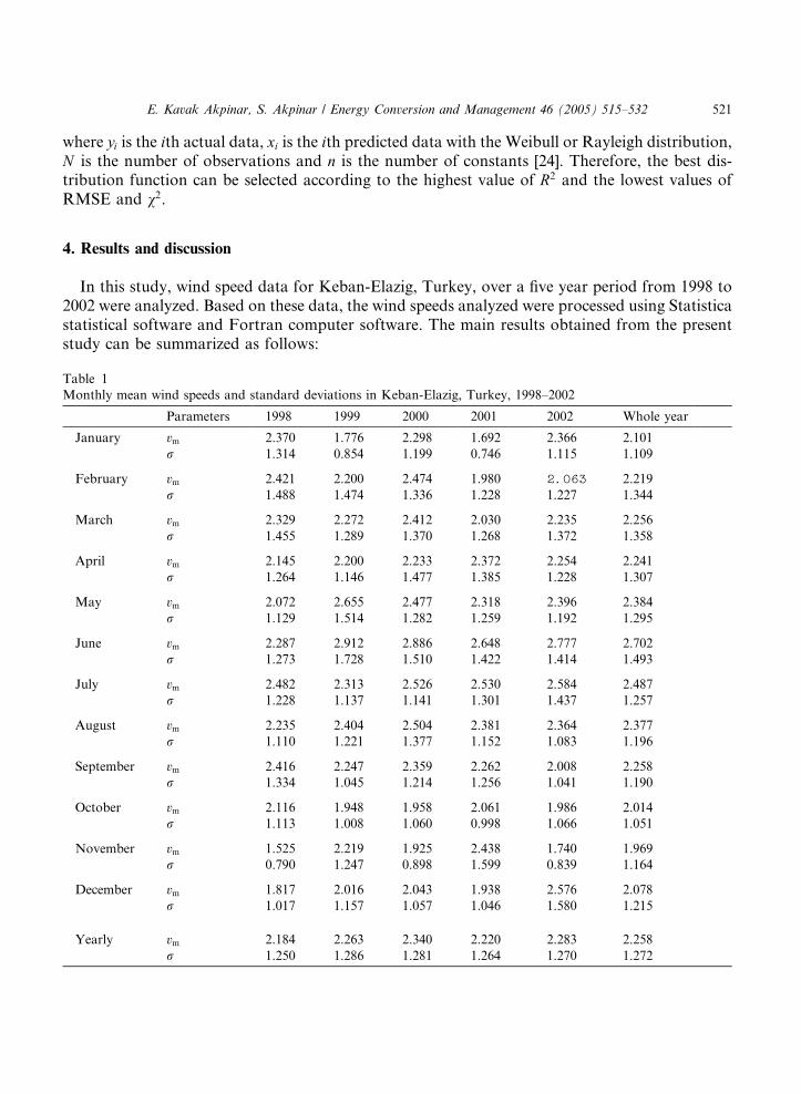
Table 1

Monthly mean wind speeds and standard deviations in Keban-Elazig, Turkey, 1998–2002

Parameters 1998 1999 2000 2001 2002 Whole year

January vm 2.370 1.776 2.298 1.692 2.366 2.101

r 1.314 0.854 1.199 0.746 1.115 1.109

February vm 2.421 2.200 2.474 1.980 2.063 2.219

r 1.488 1.474 1.336 1.228 1.227 1.344

March vm 2.329 2.272 2.412 2.030 2.235 2.256

r 1.455 1.289 1.370 1.268 1.372 1.358

April vm 2.145 2.200 2.233 2.372 2.254 2.241

r 1.264 1.146 1.477 1.385 1.228 1.307

May vm 2.072 2.655 2.477 2.318 2.396 2.384

r 1.129 1.514 1.282 1.259 1.192 1.295

June vm 2.287 2.912 2.886 2.648 2.777 2.702

r 1.273 1.728 1.510 1.422 1.414 1.493

July vm 2.482 2.313 2.526 2.530 2.584 2.487

r 1.228 1.137 1.141 1.301 1.437 1.257

August vm 2.235 2.404 2.504 2.381 2.364 2.377

r 1.110 1.221 1.377 1.152 1.083 1.196

September vm 2.416 2.247 2.359 2.262 2.008 2.258

r 1.334 1.045 1.214 1.256 1.041 1.190

October vm 2.116 1.948 1.958 2.061 1.986 2.014

r 1.113 1.008 1.060 0.998 1.066 1.051

November vm 1.525 2.219 1.925 2.438 1.740 1.969

r 0.790 1.247 0.898 1.599 0.839 1.164

December vm 1.817 2.016 2.043 1.938 2.576 2.078

r 1.017 1.157 1.057 1.046 1.580 1.215

Yearly vm 2.184 2.263 2.340 2.220 2.283 2.258

r 1.250 1.286 1.281 1.264 1.270 1.272

0

0.1

0.2

0.3

0.4

0.5

0.6

0.7

0.8

0.9

1

0 2 3 4 5 6 7 8 9 10 11

Wind speed (m/s)

Cum

ulat

ive

dens

ity JanuaryFebruaryMarchAprilMayJuneJulyAugustSeptemberOctoberNovemberDecember

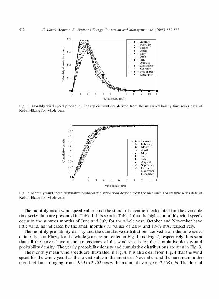
Fig. 2. Monthly wind speed cumulative probability distributions derived from the measured hourly time series data of

Keban-Elazig for whole year.

0

0.1

0.2

0.3

0.4

0 2 3 4 5 6 7 8 9 10 11

Wind speed (m/s)

Prob

abili

ty d

ensi

ty f

unct

ions

JanuaryFebruaryMarchAprilMayJuneJulyAugustSeptemberOctoberNovemberDecember

1

Fig. 1. Monthly wind speed probability density distributions derived from the measured hourly time series data of

Keban-Elazig for whole year.


The monthly mean wind speed values and the standard deviations calculated for the availabletime series data are presented in Table 1. It is seen in Table 1 that the highest monthly wind speedsoccur in the summer months of June and July for the whole year. October and November havelittle wind, as indicated by the small monthly vm values of 2.014 and 1.969 m/s, respectively.

The monthly probability density and the cumulative distributions derived from the time seriesdata of Keban-Elazig for the whole year are presented in Fig. 1 and Fig. 2, respectively. It is seenthat all the curves have a similar tendency of the wind speeds for the cumulative density andprobability density. The yearly probability density and cumulative distributions are seen in Fig. 3.

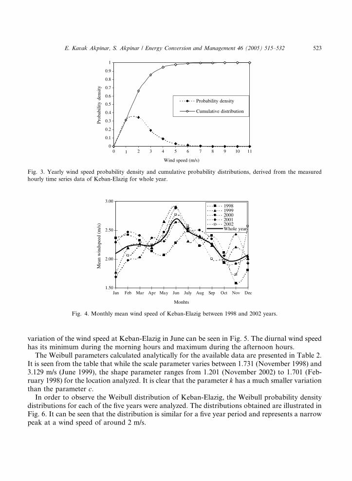
The monthly mean wind speeds are illustrated in Fig. 4. It is also clear from Fig. 4 that the windspeed for the whole year has the lowest value in the month of November and the maximum in themonth of June, ranging from 1.969 to 2.702 m/s with an annual average of 2.258 m/s. The diurnal

1.50

2.00

2.50

3.00

Jan Feb Mar Apr May Jun July Aug Sep Oct Nov Dec

Monhts

Mea

n w

inds

peed

(m

/s)

19981999200020012002Whole year

Fig. 4. Monthly mean wind speed of Keban-Elazig between 1998 and 2002 years.

0

0.1

0.2

0.3

0.4

0.5

0.6

0.7

0.8

0.9

1

0 2 3 4 5 6 7 8 9 10 11

Wind speed (m/s)

Prob

abili

ty d

ensi

tyProbability density

Cumulative distribution

1

Fig. 3. Yearly wind speed probability density and cumulative probability distributions, derived from the measured

hourly time series data of Keban-Elazig for whole year.


variation of the wind speed at Keban-Elazig in June can be seen in Fig. 5. The diurnal wind speedhas its minimum during the morning hours and maximum during the afternoon hours.

The Weibull parameters calculated analytically for the available data are presented in Table 2.It is seen from the table that while the scale parameter varies between 1.731 (November 1998) and3.129 m/s (June 1999), the shape parameter ranges from 1.201 (November 2002) to 1.701 (Feb-ruary 1998) for the location analyzed. It is clear that the parameter k has a much smaller variationthan the parameter c.

In order to observe the Weibull distribution of Keban-Elazig, the Weibull probability densitydistributions for each of the five years were analyzed. The distributions obtained are illustrated inFig. 6. It can be seen that the distribution is similar for a five year period and represents a narrowpeak at a wind speed of around 2 m/s.

1

1.5

2

2.5

3

3.5

0 2 4 6 8 10 12 14 16 18 20 22 24

Hour of day

Mea

n w

ind

spee

d (m

/s)

19981999200020012002Whole year

Fig. 5. Diurnal variation of wind speed in Keban-Elazig for June between 1998 and 2002 years.


For the purpose of calculating seasonal mean wind speeds, the months in each of the fourseasons in the northern hemisphere are generally divided as follows: (a) winter: December, Jan-uary and February; (b) spring: March, April and May; (c) summer: June, July and August and (d)autumn: September, October and November. A comparison of the seasonal Weibull probabilitydensity functions is illustrated in Fig. 7. In general, the values of the scale parameters are lowduring the winter and autumn and high during the summer.

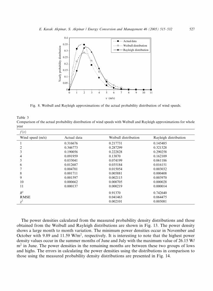
The Weibull and Rayleigh approximations of the actual probability density distribution ofwind speeds for the whole year are shown in Fig. 8, while a comparison of the two approximationswith the actual probability distribution is given in Table 3. As can be seen in Table 3, the highestR2 value was obtained by using the Weibull distribution. However, the results have shown that theRMSE and v2 values of the Weibull distribution are lower than the values obtained by theRayleigh distribution. As result, the Weibull approximation is found to be the most accuratedistribution according to the highest value of R2 and the lowest values of RMSE and v2. Fur-thermore, the monthly probability density distributions obtained from the Weibull and Rayleighdistributions were compared to the measured distributions to study their suitability. The corre-lation coefficient values are used as the measure of goodness of fit of the probability densitydistributions obtained from the Weibull and Rayleigh distributions. The correlation coefficientvalues are presented in Fig. 9 on a monthly basis for the Keban-Elazig data. The coefficient valuesrange from 0.9123 to 0.9531 for the Weibull distribution, while they vary between 0.6315 and0.8693 for the Rayleigh distributions. The month to month comparison shows that the Weibulldistribution returns higher coefficient values for all the months than the Rayleigh distribution,indicating a better fit to the measured probability density distributions.

The power density distributions are presented in Fig. 10. As seen in Fig. 10, these discrepanciesin the probability density distributions have no effect on the wind power density, since the cor-responding wind speeds are not high enough for electricity production. The most energy pro-duction is obtained at the wind speed interval of 3–4 m/s. Even though this wind speed range onlymakes up about 10% of the whole wind speed spectrum, over 30% of the total energy is produced

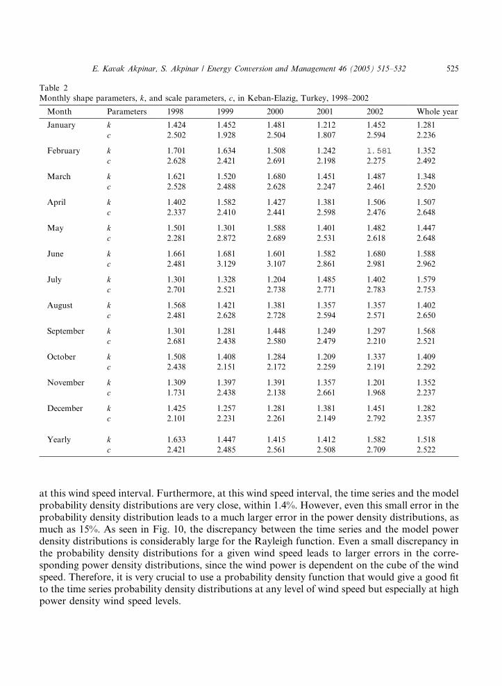
Table 2

Monthly shape parameters, k, and scale parameters, c, in Keban-Elazig, Turkey, 1998–2002

Month Parameters 1998 1999 2000 2001 2002 Whole year

January k 1.424 1.452 1.481 1.212 1.452 1.281

c 2.502 1.928 2.504 1.807 2.594 2.236

February k 1.701 1.634 1.508 1.242 1.581 1.352

c 2.628 2.421 2.691 2.198 2.275 2.492

March k 1.621 1.520 1.680 1.451 1.487 1.348

c 2.528 2.488 2.628 2.247 2.461 2.520

April k 1.402 1.582 1.427 1.381 1.506 1.507

c 2.337 2.410 2.441 2.598 2.476 2.648

May k 1.501 1.301 1.588 1.401 1.482 1.447

c 2.281 2.872 2.689 2.531 2.618 2.648

June k 1.661 1.681 1.601 1.582 1.680 1.588

c 2.481 3.129 3.107 2.861 2.981 2.962

July k 1.301 1.328 1.204 1.485 1.402 1.579

c 2.701 2.521 2.738 2.771 2.783 2.753

August k 1.568 1.421 1.381 1.357 1.357 1.402

c 2.481 2.628 2.728 2.594 2.571 2.650

September k 1.301 1.281 1.448 1.249 1.297 1.568

c 2.681 2.438 2.580 2.479 2.210 2.521

October k 1.508 1.408 1.284 1.209 1.337 1.409

c 2.438 2.151 2.172 2.259 2.191 2.292

November k 1.309 1.397 1.391 1.357 1.201 1.352

c 1.731 2.438 2.138 2.661 1.968 2.237

December k 1.425 1.257 1.281 1.381 1.451 1.282

c 2.101 2.231 2.261 2.149 2.792 2.357

Yearly k 1.633 1.447 1.415 1.412 1.582 1.518

c 2.421 2.485 2.561 2.508 2.709 2.522


at this wind speed interval. Furthermore, at this wind speed interval, the time series and the modelprobability density distributions are very close, within 1.4%. However, even this small error in theprobability density distribution leads to a much larger error in the power density distributions, asmuch as 15%. As seen in Fig. 10, the discrepancy between the time series and the model powerdensity distributions is considerably large for the Rayleigh function. Even a small discrepancy inthe probability density distributions for a given wind speed leads to larger errors in the corre-sponding power density distributions, since the wind power is dependent on the cube of the windspeed. Therefore, it is very crucial to use a probability density function that would give a good fitto the time series probability density distributions at any level of wind speed but especially at highpower density wind speed levels.

0

0.1

0.2

0.3

0 1 2 3 4 5 6 7 8 9 10 11

Wind speeds (m/s)

Prob

abili

ty d

ensi

ty f

unct

ions

1998

1999

2000

2001

2002

Fig. 6. Yearly Weibull probability density distributions for the period of 1998–2002 in Keban-Elazig.

0

0.1

0.2

0.3

0 2 3 4 5 6 7 8 9 10 11

Wind speeds (m/s)

Prob

abili

ty d

ensi

ty f

unct

ions

WinterSpringSummerAutumn

1

Fig. 7. A comparison of seasonal Weibull probability density function distributions in Keban-Elazig.


Fig. 11 illustrates the variation of yearly wind power density versus different hub height for thewhole year, while Fig. 12 illustrates the monthly wind power density for Keban-Elazig. Fig. 11shows that the mean wind speed and wind power density increase with the increase of hub height.Obviously, to obtain higher wind power, the higher hub heights are preferred. It is clear from Fig.12 that in November and October, the wind power is low but is very high in June. The two curveshave similar changing trends, but the rate of change is not the same. In addition, the yearlyWeibull parameters, yearly wind power density and yearly mean wind speed can be obtained asshown in Table 4. It is observed that the value of wind power density is low in 1998, but it is highin 2000. Similarly, Table 5 indicates the seasonal wind power density and seasonal mean windspeed in addition to the seasonal Weibull parameters. The results show that the parameters aredistinctive for the different seasons in Keban-Elazig, 1998–2002.

0

0.05

0.1

0.15

0.2

0.25

0.3

0.35

0.4

0 1 2 3 4 5 6 7 8 9 10 11

v (m/s)

Yea

rly

prob

abili

ty d

istr

ibut

ion

Actual data

Weibull distribution

Rayleigh distribution

Fig. 8. Weibull and Rayleigh approximations of the actual probability distribution of wind speeds.

Table 3

Comparison of the actual probability distribution of wind speeds with Weibull and Rayleigh approximations for whole

year

f ðvÞWind speed (m/s) Actual data Weibull distribution Rayleigh distribution

1 0.316676 0.217731 0.145485

2 0.346773 0.287299 0.321328

3 0.190056 0.222828 0.290258

4 0.091959 0.13870 0.162109

5 0.033041 0.074199 0.061186

6 0.012687 0.035184 0.016151

7 0.004701 0.015054 0.003032

8 0.001711 0.005881 0.000408

9 0.001597 0.002115 0.003970

10 0.000662 0.000705 0.000028

11 0.000137 0.000219 0.000014

R2 0.91370 0.742640

RMSE 0.041463 0.064475

v2 0.002101 0.005081


The power densities calculated from the measured probability density distributions and thoseobtained from the Weibull and Rayleigh distributions are shown in Fig. 13. The power densityshows a large month to month variation. The minimum power densities occur in November andOctober with 9.89 and 11.59 W/m2, respectively. It is interesting to note that the highest powerdensity values occur in the summer months of June and July with the maximum value of 26.15 W/m2 in June. The power densities in the remaining months are between these two groups of lowsand highs. The errors in calculating the power densities using the distributions in comparison tothose using the measured probability density distributions are presented in Fig. 14.

0

0.1

0.2

0.3

0.4

0.5

0.6

0.7

0.8

0.9

1


Month

R2

Weibull Rayleigh

Fig. 9. Correlation coefficient values obtained in fitting the actual probability density distributions with the Weibull

and Rayleigh functions.

0

1

2

3

4

5

6

7

0 1 2 3 4 5 6 7 8 9 10 11

Wind speed (m/s)

Win

d po

wer

(W/m

2 )

Actual data

Weibull distribution

Rayleigh distribution

Fig. 10. Weibull and Rayleigh approximations of the actual probability distribution of wind power densities.

2.5

2.75

3

3.25

3.5

10 20 30 40 50 60 70 80 90 100

Height (m)

Pow

er d

ensi

ty(W

/m2 )

15

17

19

21

23

Mea

n w

ind

spee

d(m

/s)

Mean wind speed

Power density

Fig. 11. Yearly power density and mean wind speed for different hub heights.


1.9

2.1

2.3

2.5

2.7


Months

Mea

n w

ind

spee

d (m

/s)

9

13.5

18

22.5

27

Mea

n w

indp

ower

(W

/m2 )

Mean windspeedMean windpower

Fig. 12. Monthly wind power density and mean wind speed.

Table 4

Yearly wind characteristics in Keban-Elazig, Turkey

Year vm (m/s) k c (m/s) vMP (m/s) VMax E (m/s) P (W/m2)

1998 2.184 1.633 2.421 1.355 3.950 14.366

1999 2.263 1.447 2.485 1.103 4.527 15.997

2000 2.340 1.415 2.561 1.076 4.773 16.555

2001 2.220 1.412 2.508 1.048 4.684 15.126

2002 2.283 1.582 2.709 1.439 4.541 15.922

Table 5

Seasonal wind characteristics in Keban-Elazig, Turkey

Season vm (m/s) k c (m/s) vMP (m/s) vMaxE (m/s) P (W/m2)

Winter 2.130 1.402 2.412 0.989 4.539 13.474

Spring 2.294 1.387 2.478 0.987 4.716 16.681

Summer 2.519 1.552 2.797 1.436 5.768 19.859

Autumn 2.080 1.352 2.356 0.863 4.572 11.845

Whole year 2.258 1.518 2.522 1.242 4.387 15.603


The Weibull model returns smaller error values in calculating the power density when com-pared to the Rayleigh model. The highest error values occur in October and November with26.39% and 26.07% for the Weibull model, respectively. The power density is estimated by theWeibull model with a very small error value of 6.28% in April. The yearly average error value incalculating the power density using the Weibull function is 13.64%. The monthly analysis showsthat the error values in calculating the power density using the Rayleigh model are relativelyhigher, over 25% in some months, such as November and December. Even the smallest error in

0

10

20

30


Month

Pow

er d

ensi

ty (

W/m

2 )

Actual dataWeibull distributionRayleigh distribution

Fig. 13. Wind power density obtained from the actual data versus those obtained from the Weibull and Rayleigh

models on a monthly basis.

-30%

-20%

-10%

0%

10%

20%

30%


Err

ors

(%)

Weibull

Rayleigh

Fig. 14. Error values in calculating the wind power density obtained from the Weibull and Rayleigh models in reference

to the wind power density obtained from the actual data, on monthly basis.


the power density calculation using the Rayleigh model is 11.54%. The yearly average error valuein estimating the power density using the Rayleigh model is 18.60%.

5. Conclusions

In the present study, the hourly measured time series wind speed data of Keban-Elazig havebeen statistically analyzed. The probability density distributions and power density distributionshave been derived from the time series data and the distributional parameters were identified. Twoprobability density functions have been fitted to the measured probability distributions on amonthly basis. The wind energy potential of the location has been studied based on the Weibulland the Rayleigh models. The most important outcomes of the study can be summarized asfollows:


1. The Keban-Elazig station where the Turkish State Meteorological Service is located, presentspoor wind characteristics. This is shown by the low monthly and yearly mean wind speed andpower density values for the whole year.

2. The yearly average wind power density value is 15.603 W/m2 for the whole year. Therefore, thisparticular site is not ideal for grid connected applications. This level of power density may beadequate for non-connected electrical and mechanical applications, such as battery chargingand water pumping.

3. However, the diurnal variations of the wind speed and the wind power density may show a sig-nificant variation.

4. The Weibull distribution is better in fitting the measured monthly probability density distribu-tions than the Rayleigh distribution for the whole year. This is shown from the monthly cor-relation coefficient values of the fits.

5. The Weibull distribution provided better power density estimations in all 12 months than theRayleigh distribution.

References

[1] K€ose R. An evaluation of wind energy potential as a power generation source in K€utahya, Turkey. Energy Conv

Mgmt 2003;45:1631–41.

[2] Sen Z, Sahin AD. Regional wind energy evaluation in some parts of Turkey. J Wind Eng Ind Aerodynam 1998;

74–76:345–53.

[3] Celik AN. A statistical analysis of wind power density based on the Weibull and Rayleigh models at the southern

region of Turkey. Renew Energy 2003;29:593–604.

[4] Celik AN. Weibull representative compressed wind speed data for energy and performance calculations of wind

energy systems. Energy Conv Mgmt 2003;44:3057–72.

[5] Ulgen K, Hepbasli A. Determination of Weibull parameters for wind energy analysis of Izmir, Turkey. Int J

Energy Res 2002;26:494–506.

[6] Ozgener O, Hepbasli A. Current status and future directions of wind energy applications in Turkey. Energy

Sources 2002;24:1117–29.

[7] Hepbasli A, Ozgener O. A review on the development of wind energy in Turkey. Renew Sustain Energy Rev

2004;8(3):257–76.

[8] Shabbaneh R, Hasan A. Wind energy potential in Palestina. Renew Energy 1997;11:479–83.

[9] Mayhoub AB, Azzam A. A survey on the assessment of wind energy potential in Egypt. Renew Energy

1997;11:235–47.

[10] Deaves DM, Lines IG. On the fitting of low mean wind speed data to the Weibull distribution. J Wind Eng Ind

Aerodynam 1997;66:169–78.

[11] Algifri AH. Wind energy potential in Aden-Yemen. Renew Energy 1998;13:255–60.

[12] Sahin AZ, Aksakal A. Wind power energy potential at Northeastern region of Saudi Arabia. Renew Energy

1998;14:435–40.

[13] Persaud S, Flynn D, Fox B. Potential for wind generation on the Guyana coastlands. Renew Energy 1999;18:

175–89.

[14] Seguro JV, Lambert TW. Modern estimation of the parameters of the Weibull wind speed distribution for wind

energy analysis. J Wind Eng Ind Aerodynam 2000;85:75–84.

[15] Lun IYF, Lam JC. A study of Weibull parameters using long-term wind observations. Renew Energy 2000;20:

145–53.

[16] Bivona S, Burlon R, Leone C. Hourly wind speed analysis in Sicily. Renew Energy 2003;28:1371–85.

[17] Celik AN. On the distributional parameters used in assessment of the suitability of wind speed probability density

functions. Energy Conv Mgmt 2004;45:1735–47.


[18] Kose R, Ozgur MA, Erbas O, Tugcu A. The analysis of wind data and wind energy potential in Kutahya, Turkey.

Renew Sustain Energy Rev 2004;8(3):277–88.

[19] Karsli VM, Gecit C. An investigation on wind power potential of Nurda�gı-Gaziantep, Turkey. Renew Energy

2003;28:823–30.

[20] Oztopal A, Sahin AD, Akgun N, Sen Z. On the regional wind energy potential of Turkey. Energy 2000;25:189–200.

[21] Durak M, Sen Z. Wind power potential in Turkey and Akhisar case study. Renew Energy 2002;25:463–72.

[22] Sahin AD. Hourly wind velocity exceedence maps of Turkey. Energy Conv Mgmt 2003;44:549–57.

[23] Chang TJ, Wu YT, Hsu HY, Chu CR, Liao CM. Assessment of wind characteristics and wind turbine

characteristics in Taiwan. Renew Energy 2003;28:851–71.

[24] Holman JP. Experimental methods for engineers. McGraw-Hill Book Company; 1971. p. 37–52.

statistical analysis of windspeed data

Documents

wind farms

wind speed data of keban

distribution of wind

akpinar energy conversion

energy of theenergy

turkish ministry of

kavak akpinar

important parameter