statistical analysis in the lexis ... - bendix carstensen · such datasets can be read into r with...
TRANSCRIPT

Statistical Analysis in theLexis Diagram:
Age-Period-Cohort models
Max Plack Insitute of Demographic Research, Rostock2-6 May 2016
http://BendixCarstensen.com/APC/MPIDR-2016
1.0
Compiled Friday 29th April, 2016, 21:28from: /home/bendix/teach/APC/MPIDR.2016/pracs/pracs.tex
Bendix Carstensen Steno Diabetes Center, Gentofte, Denmark& Department of Biostatistics, University of Copenhagen
www.BendixCarstensen.com
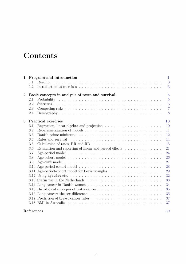
Contents
1 Program and introduction 11.1 Reading . . . . . . . . . . . . . . . . . . . . . . . . . . . . . . . . . . . . . . 31.2 Introduction to exercises . . . . . . . . . . . . . . . . . . . . . . . . . . . . . 3
2 Basic concepts in analysis of rates and survival 52.1 Probability . . . . . . . . . . . . . . . . . . . . . . . . . . . . . . . . . . . . 52.2 Statistics . . . . . . . . . . . . . . . . . . . . . . . . . . . . . . . . . . . . . . 62.3 Competing risks . . . . . . . . . . . . . . . . . . . . . . . . . . . . . . . . . . 72.4 Demography . . . . . . . . . . . . . . . . . . . . . . . . . . . . . . . . . . . . 8
3 Practical exercises 103.1 Regression, linear algebra and projection . . . . . . . . . . . . . . . . . . . . 103.2 Reparametrization of models . . . . . . . . . . . . . . . . . . . . . . . . . . . 113.3 Danish prime ministers . . . . . . . . . . . . . . . . . . . . . . . . . . . . . . 123.4 Rates and survival . . . . . . . . . . . . . . . . . . . . . . . . . . . . . . . . 143.5 Calculation of rates, RR and RD . . . . . . . . . . . . . . . . . . . . . . . . 153.6 Estimation and reporting of linear and curved effects . . . . . . . . . . . . . 213.7 Age-period model . . . . . . . . . . . . . . . . . . . . . . . . . . . . . . . . . 243.8 Age-cohort model . . . . . . . . . . . . . . . . . . . . . . . . . . . . . . . . . 263.9 Age-drift model . . . . . . . . . . . . . . . . . . . . . . . . . . . . . . . . . . 273.10 Age-period-cohort model . . . . . . . . . . . . . . . . . . . . . . . . . . . . . 283.11 Age-period-cohort model for Lexis triangles . . . . . . . . . . . . . . . . . . 293.12 Using apc.fit etc. . . . . . . . . . . . . . . . . . . . . . . . . . . . . . . . . 323.13 Statin use in the Netherlands . . . . . . . . . . . . . . . . . . . . . . . . . . 333.14 Lung cancer in Danish women . . . . . . . . . . . . . . . . . . . . . . . . . . 343.15 Histological subtypes of testis cancer . . . . . . . . . . . . . . . . . . . . . . 353.16 Lung cancer: the sex difference . . . . . . . . . . . . . . . . . . . . . . . . . 363.17 Prediction of breast cancer rates . . . . . . . . . . . . . . . . . . . . . . . . . 373.18 BMI in Australia . . . . . . . . . . . . . . . . . . . . . . . . . . . . . . . . . 37
References 39
ii

Chapter 1
Program and introduction
Course program
As the general rule, the daily program will have one lecture and one practical each morningand each afternoon.
Lectures will be between 45 and 90 minutes; normally with one or two breaks.Occasionally you will be asked to do small practical in the middle of the lectures.
The practicals will follow the lecture to fill the 3-hour slot. Sometimes we may need topush over some of the practical computing to take a bit of the beginning of the next slot.
The general rule is that there will be a walk-through of practicals after you have had achange to have a go at it yourself.
Monday 2nd
09:00 – 09:15 Welcome and introduction.09:15 – 12:15 Morning slot:
– L1: Follow-up time and rates from register data surv-rate
– Lexis machinery in Epi lifetable
– Follow-up time and rates from population data tab-mod
– P1: Regression, linear algebra and reparametrization– Danish prime ministers pm
13:15 – 16:15 Afternoon slot:– L2: Likelihood for rates: Cox and Poisson– Cox as limit of the Poisson WntCma
– Poisson model for rates: Factor models– Practical handling of linear contrasts in R using ci.lin() tab-mod
– P2: Rates and survival, RR and RD– Linear and curved effects
1

2 APC models
Tuesday 3rd
09:00 – 09:30 Recap of Monday09:30 – 12:15 Morning slot:
– L3: The age-period and the age-cohort model. AP-AC– The Age-drift model– P3: Age-period model age-per– Age-cohort model age-coh– Age-drift model age-drift
13:15 – 16:15 Afternoon slot:– L4: The Age-period-cohort model– Parametrizations– Lexis triangles– P4: Age-period-cohort model– Using apc.fit
Wednesday 4th
09:00 – 09:30 Recap of Tuesday09:30 – 12:15 Morning slot:
– L5: Parametrization revisited: The general case.– The Lee-Carter model– P5: Age-period-cohort model for triangles– L5: The implementation of apc.fit.– Parametrizations.– The residual parametrization.– P5: Lee-Carter: Lung cancer in Danish women
13:15 – 16:15 Afternoon slot:– L6: Several rates compared with APC-models:– Estimation and reporting of effects.– Parametrization options for several rates.– P6: Lung cancer differences by sex lung-sex
Thursday 5th
09:00 – 16:00 Study free: Working with the assignments.

APC models 1.1 Reading 3
Friday 6th
09:00 – 09:30 Recap of Wednesday09:30 – 12:15 Morning slot:
– L7: Predictions based on APC models– Managing splines for prediction– P7: Predicting lung cancer lung-pred– Predicting breast cancer breast-pred
13:15 – 16:00 Afternoon slot:– L8: APC-models for continuous outcome– P8: BMI in Australia
16:00 – 16:15 Wrapping up, closure, evaluation and farewell
1.1 Reading
It would be helpful if you had read the papers which cover the essentials of the models thatwe will cover: [1, 2, 3, 4]
1.2 Introduction to exercises
Most of the following exercises all require basic skills in computing, in R, in particular theuse of the graphical facilities.
1.2.1 Datasets and how to access them.
All the datasets for the exercises in this section are in the folder APC\data. This can beaccessed through the homepage of the course, as:http://BendixCarstensen.com/APC/data.
The datasets with .txt extension are plain text files where variable names are found inthe first line. Such datasets can be read into R with the command read.table
1.2.2 R-functions and packages
Most functions for this course (and several more) are supplied in the R-package Epi, whichcan be downloaded from CRAN (on the R-website). It is also recommended that you getthe packages demography and ilc.
> library( Epi )> sessionInfo()
The latter command will list the attached packages and their version numbers. Yur versionof Epi should be at least 2.3.
1.2.3 Solutions
This document also contains some suggestions for solutions of the assignments. Theyshould not be taken as the only possible solutions to the practicals.

4 1.2 Introduction to exercises APC models
It is a good idea to give it a shot to do the practicals before you look in the solutions.However, the odd solution proposal may contain a twist to the analyses that you may finduseful. Any suggestions for improving the solutions would be most welcome.
The R-code used in the solutions is available in the folderhttp://bendixcarstensen.com/APC/MPIDR-2016/R/, the filenames are shown at the topof each of the solution sections.

Chapter 2
Basic concepts in analysis of rates andsurvival
The following is a summary of relations between various quantities used in analysis offollow-up studies. They are ubiquitous in the analysis and reporting of results. Hence it isimportant to be familiar with all of them and the relation between them.
2.1 Probability
Survival function:
S(t) = P {survival at least till t}= P {T > t} = 1− P {T ≤ t} = 1− F (t)
Conditional survival function:
S(t|tentry) = P {survival at least till t| alive at tentry}= S(t)/S(tentry)
Cumulative distribution function of death times (cumulative risk):
F (t) = P {death before t}= P {T ≤ t} = 1− S(t)
Density function of death times:
f(t) = limh→0
P {death in (t, t+ h)} /h = limh→0
F (t+ h)− F (t)
h= F ′(t)
Intensity:
λ(t) = limh→0
P {event in (t, t+ h] | alive at t} /h
= limh→0
F (t+ h)− F (t)
S(t)h=f(t)
S(t)
= limh→0− S(t+ h)− S(t)
S(t)h= − d logS(t)
dt
5

6 2.2 Statistics APC models
The intensity is also known as the hazard function, hazard rate, mortality/morbidityrate or simply “rate”.
Note that f and λ are scaled quantities, they have dimension time−1.
Relationships between terms:
− d logS(t)
dt= λ(t)
m
S(t) = exp
(−∫ t
0
λ(u) du
)= exp
(−Λ(t)
)The quantity Λ(t) =
∫ t
0λ(s) ds is called the integrated intensity or the cumulative
rate. It is not an intensity (rate), it is dimensionless, despite its name.
λ(t) = − d log(S(t))
dt= −S
′(t)
S(t)=
F ′(t)
1− F (t)=f(t)
S(t)
The cumulative risk of an event (to time t) is:
F (t) = P {Event before time t} =
∫ t
0
λ(u)S(u) du = 1− S(t) = 1− e−Λ(t)
For small |x| (< 0.05), we have that 1− e−x ≈ x, so for small values of the integratedintensity:
Cumulative risk to time t ≈ Λ(t) = Cumulative rate
2.2 Statistics
Likelihood contribution from follow up of one person:The likelihood from a number of small pieces of follow-up from one individual is aproduct of conditional probabilities:
P {event at t4|entry at t0} = P {survive (t0, t1)| alive at t0} ×P {survive (t1, t2)| alive at t1} ×P {survive (t2, t3)| alive at t2} ×P {event at t4| alive at t3}
Each term in this expression corresponds to one empirical rate1
(d, y) = (#deaths,#risk time), i.e. the data obtained from the follow-up of oneperson in the interval of length y. Each person can contribute many empirical rates,most with d = 0; d can only be 1 for the last empirical rate for a person.
Log-likelihood for one empirical rate (d, y):
`(λ) = d log(λ)− λy
This is under the assumption that the rate (λ) is constant over the interval that theempirical rate refers to.
1This is a concept coined by BxC, and so is not necessarily generally recognized.

APC models 2.3 Competing risks 7
Log-likelihood for several persons. Adding log-likelihoods from a group of persons(only contributions with identical rates) gives:
D log(λ)− λY,
where Y is the total follow-up time, and D is the total number of failures.
Note: The Poisson log-likelihood for an observation D with mean λY is:
D log(λY )− λY = D log(λ) +D log(Y )− λY
The term D log(Y ) does not involve the parameter λ, so the likelihood for anobserved rate can be maximized by pretending that the no. of cases D is Poissonwith mean λY . But this does not imply that D follows a Poisson-distribution. It isentirely a likelihood based computational convenience. Anything that is notlikelihood based is not justified.
A linear model for the log-rate, log(λ) = Xβ implies that
λY = exp(log(λ) + log(Y )
)= exp
(Xβ + log(Y )
)Therefore, in order to get a linear model for log(λ) we must require that log(Y )appear as a variable in the model for D ∼ (λY ) with the regression coefficient fixedto 1, a so-called offset-term in the linear predictor.
2.3 Competing risks
Competing risks: If there is more than one, say 3, causes of death, occurring with(cause-specific) rates λ1, λ2, λ3, that is:
λc(a) = limh→0
P {death from cause c in (a, a+ h] | alive at a} /h, c = 1, 2, 3
The survival function is then:
S(a) = exp
(−∫ a
0
λ1(u) + λ2(u) + λ3(u) du
)because you have to escape all 3 causes of death. The probability of dying from cause1 before age a (the cause-specific cumulative risk) is:
P {dead from cause 1 at a} =
∫ a
0
λ1(u)S(u) du 6= 1− exp
(−∫ a
0
λ1(u) du
)The term exp(−
∫ a
0λ1(u) du) is sometimes referred to as the “cause-specific survival”,
but it does not have any probabilistic interpretation in the real world. It is thesurvival under the assumption that only cause 1 existed and that the mortality ratefrom this cause was the same as when the other causes were present too.
Together with the survival function, the cause-specific cumulative risks represent aclassification of the population at any time in those alive and those dead from causes1, 2 and 3 respectively:
1 = S(a) +
∫ a
0
λ1(u)S(u) du+
∫ a
0
λ2(u)S(u) du+
∫ a
0
λ3(u)S(u) du, ∀a

8 2.4 Demography APC models
Subdistribution hazard Fine and Gray defined models for the so-called subdistributionhazard. Recall the relationship between between the hazard (λ) and the cumulativerisk (F ):
λ(a) = −d log
(S(a)
)da
= −d log
(1− F (a)
)da
When more competing causes of death are present the Fine and Gray idea is to usethis transformation to the cause-specific cumulative risk for cause 1, say:
λ1(a) = −d log
(1− F1(a)
)da
This is what is called the subdistribution hazard, it depends on the survival functionS, which depends on all the cause-specific hazards:
F1(a) = P {dead from cause 1 at a} =
∫ a
0
λ1(u)S(u) du
The subdistribution hazard is merely a transformation of the cause-specificcumulative risk. Namely the same transformation which in the single-cause casetransforms the cumulative risk to the hazard.
2.4 Demography
Expected residual lifetime: The expected lifetime (at birth) is simply the variable age(a) integrated with respect to the distribution of age at death:
EL =
∫ ∞0
af(a) da
where f is the density of the distribution of lifetime (age at death).
The relation between the density f and the survival function S is f(a) = −S ′(a), sointegration by parts gives:
EL =
∫ ∞0
a(−S ′(a)
)da = −
[aS(a)
]∞0
+
∫ ∞0
S(a) da
The first of the resulting terms is 0 because S(a) is 0 at the upper limit and a bydefinition is 0 at the lower limit.
Hence the expected lifetime can be computed as the integral of the survival function.
The expected residual lifetime at age a is calculated as the integral of the conditionalsurvival function for a person aged a:
EL(a) =
∫ ∞a
S(u)/S(a) du
Lifetime lost due to a disease is the difference between the expected residual lifetime fora diseased person and a non-diseased (well) person at the same age. So all that isneeded is a(n estimate of the) survival function in each of the two groups.
LL(a) =
∫ ∞a
SWell(u)/SWell(a)− SDiseased(u)/SDiseased(a) du
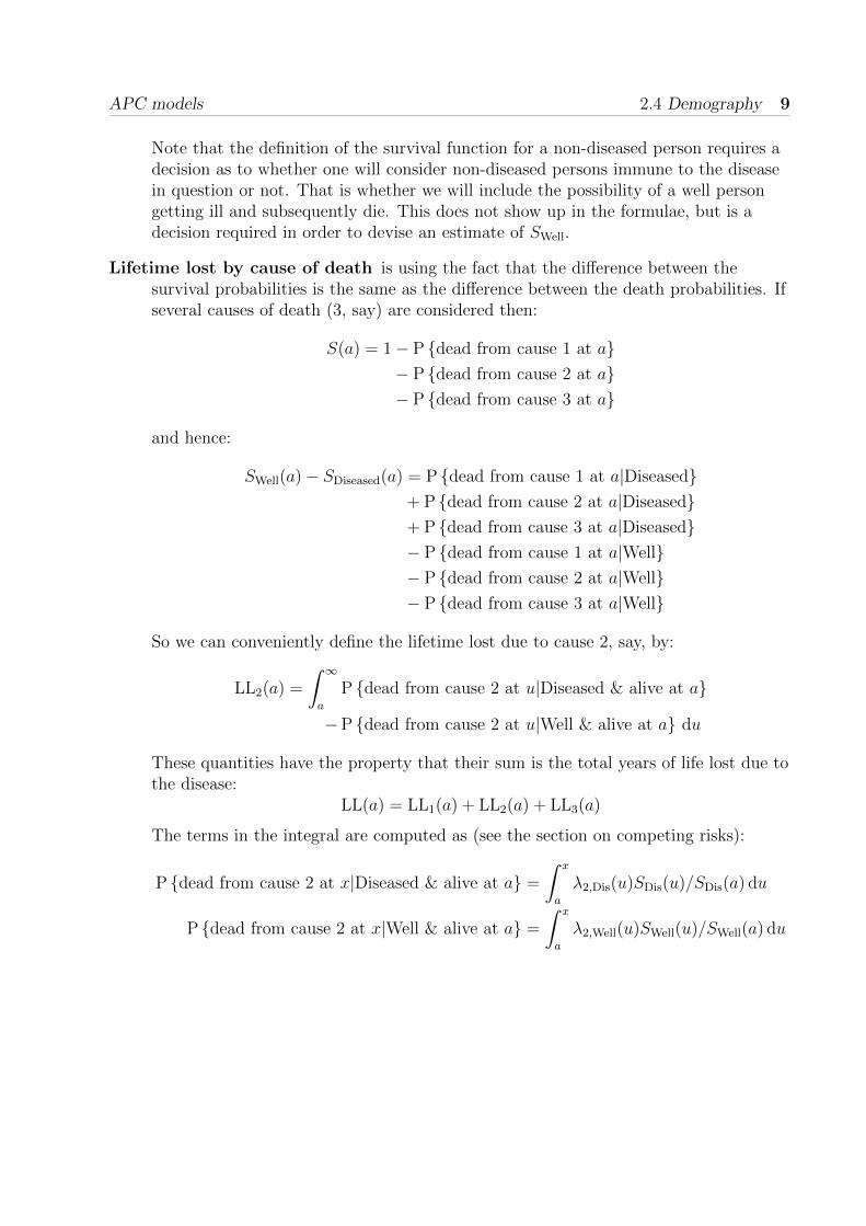
APC models 2.4 Demography 9
Note that the definition of the survival function for a non-diseased person requires adecision as to whether one will consider non-diseased persons immune to the diseasein question or not. That is whether we will include the possibility of a well persongetting ill and subsequently die. This does not show up in the formulae, but is adecision required in order to devise an estimate of SWell.
Lifetime lost by cause of death is using the fact that the difference between thesurvival probabilities is the same as the difference between the death probabilities. Ifseveral causes of death (3, say) are considered then:
S(a) = 1− P {dead from cause 1 at a}− P {dead from cause 2 at a}− P {dead from cause 3 at a}
and hence:
SWell(a)− SDiseased(a) = P {dead from cause 1 at a|Diseased}+ P {dead from cause 2 at a|Diseased}+ P {dead from cause 3 at a|Diseased}− P {dead from cause 1 at a|Well}− P {dead from cause 2 at a|Well}− P {dead from cause 3 at a|Well}
So we can conveniently define the lifetime lost due to cause 2, say, by:
LL2(a) =
∫ ∞a
P {dead from cause 2 at u|Diseased & alive at a}
−P {dead from cause 2 at u|Well & alive at a} du
These quantities have the property that their sum is the total years of life lost due tothe disease:
LL(a) = LL1(a) + LL2(a) + LL3(a)
The terms in the integral are computed as (see the section on competing risks):
P {dead from cause 2 at x|Diseased & alive at a} =
∫ x
a
λ2,Dis(u)SDis(u)/SDis(a) du
P {dead from cause 2 at x|Well & alive at a} =
∫ x
a
λ2,Well(u)SWell(u)/SWell(a) du

Chapter 3
Practical exercises
3.1 Regression, linear algebra and projection
This exercise is aimed at reminding you about the linear algebra behind linear models.Therefor we use artificial data
1. First generate a continuous variable x, and a factor f on 3 levels, each with 100 units,say:
x <- runif(100,20,50)f <- factor( sample(letters[1:3],100,replace=T) )xtable( f )
Then generate a response variable y by some function (the exact shape isimmaterial):
y <- 0.2*x + 0.02*(x-25)^2 + 3*as.integer(f) + rnorm(100,0,1)plot( x, y, col=f, pch=16 )
2. Now fit the same model using lm, so this should get your parameter estimates back(almost):
mm <- lm( y ~ x + I(x^2) + f )summary( mm )
3. Now verify that you get the same results using the matrix formulae. You will firsthave to generate the design matrix:
X <- cbind( 1, x, x^2, f=="b", f=="c" )
Recall that the matrix formula for the estimates is:
β = (X ′X)−1X ′y
To make this calculation explicitly in R you will need the transpose t() and thematrix inversion solve() functions, as well as the matrix multiplication operator %*%.
An explicit calculation then gives:
bb <- solve( t(X) %*% X ) %*% t(X) %*% ycbind( bb, coef(mm) )
10

APC models 3.2 Reparametrization of models 11
3.2 Reparametrization of models
This exercise is aimed at showing you how to reparametrize a model: Suppose you have amodel parametrized by the linear predictor Xβ, but that you really wanted theparametrization Aγ, where the columns of X and A span the same linear space.
So Xβ = Aγ, and we assume that both X and A are of full rank,dim(X) = dim(A) = n× p, say.
We want to find γ given that we know Xβ and that Xβ = Aγ. Since we have thatp < n, we have that A−A = I, by the properties of G-inverses, and hence:
γ = A−Aγ = A−Xβ
1. try to generate a dataset with a response hat is normally distributed in three groups,and then fit the model using the “usual” parametrization:
f <- factor( sample(letters[1:3],20,replace=T) )y <- 5+2*as.integer(f) + rnorm(20,0,1)mm <- lm( y ~ f )library( Epi )ci.lin( mm )
2. Set up the model matrix X for this regression, and versify that you get the sameresults by entering X as regression in lm
( X <- cbind( 1, f=="b", f=="c" ) )ci.lin( lm( y ~ X-1 ) )
3. Now suppose you want a parametrization with the last level as reference instead. Youcould then easily convert the parameters, but use the formulae from above to do it,by first setting up A corresponding to the desired parametrization, and then usingginv from the MASS library:
library( MASS )( A <- cbind( 1, f=="a", f=="b" ) )ginv(A) %*% Xginv(A) %*% X %*% ci.lin( mm )[,1]
4. Verify that you get the results you expect:
( X <- cbind( 1, f=="b", f=="c" ) )( A <- cbind( 1, f=="a", f=="b" ) )ginv(A) %*% X
5. Try to obtain the conversion from the parametrization with an intercept and twocontrasts to the parametrization with a separate level in each group by constructingthe matrices using the model.matrix function.
( X <- model.matrix( ~f ) )( A <- model.matrix( ~f-1 ) )ginv(A) %*% X
The essences of these calculations are:

12 3.3 Danish prime ministers APC models
• Given that you have a set of fitted values in a model (in casu y = Xβ) and you wantthe parameter estimates you would get if you had used the model matrix A. Thenthey are γ = A−y = A−Xβ.
• Given that you have a set of parameters β, from fitting a model with design matrixX, and you would like the parameters γ, you would have got had you used the modelmatrix A. Then they are γ = A−Xβ.
3.3 Danish prime ministers
The following table shows all Danish prime ministers in office since the war. They areordered by the period in office, hence some appear twice. Entry end exit refer to the officeof prime minister. A missing date of death means that the person was alive at 31 March2016.
Name Birth Death Entry Exit
Vilhelm Buhl 16/10/1881 18/12/1954 05/05/1945 07/11/1945Knud Kristensen 26/10/1880 29/09/1962 07/11/1945 13/11/1947Hans Hedtoft 21/04/1903 29/01/1955 13/11/1947 30/10/1950Erik Eriksen 20/11/1902 07/10/1972 30/10/1950 30/09/1953Hans Hedtoft 21/04/1903 29/01/1955 30/09/1953 29/01/1955H C Hansen 08/11/1906 19/02/1960 01/02/1955 19/02/1960Viggo Kampmann 21/07/1910 03/06/1976 21/02/1960 03/09/1962Jens Otto Kragh 15/09/1914 22/06/1978 03/09/1962 02/02/1968Hilmar Baunsgaard 26/02/1920 30/06/1989 02/02/1968 11/10/1971Jens Otto Kragh 15/09/1914 22/06/1978 11/10/1971 05/10/1972Anker Jorgensen 13/07/1922 20/03/2016 05/10/1972 19/12/1973Poul Hartling 14/08/1914 30/04/2000 19/12/1973 13/02/1975Anker Jorgensen 13/07/1922 20/03/2016 13/02/1975 10/09/1982Poul Schluter 03/04/1929 . 10/09/1982 25/01/1993Poul Nyrup Rasmussen 15/06/1943 . 25/01/1993 27/11/2001Anders Fogh Rasmussen 26/01/1953 . 27/11/2001 05/04/2007Lars Løkke Rasmussen 15/05/1964 . 21/01/2009 03/10/2011Helle Thorning-Schmidt 14/12/1966 . 03/10/2011 28/06/2015Lars Løkke Rasmussen 15/05/1964 . 28/06/2015 .
The data in the table can be found in the file pm-dk.txt.
st <- read.table( "../data/pm-dk.txt", header=T, as.is=T, na.strings="." )ststr( st )
1. Draw a Lexis diagram with life-lines of the persons, for example by using the Lexis
machinery from the Epi package:
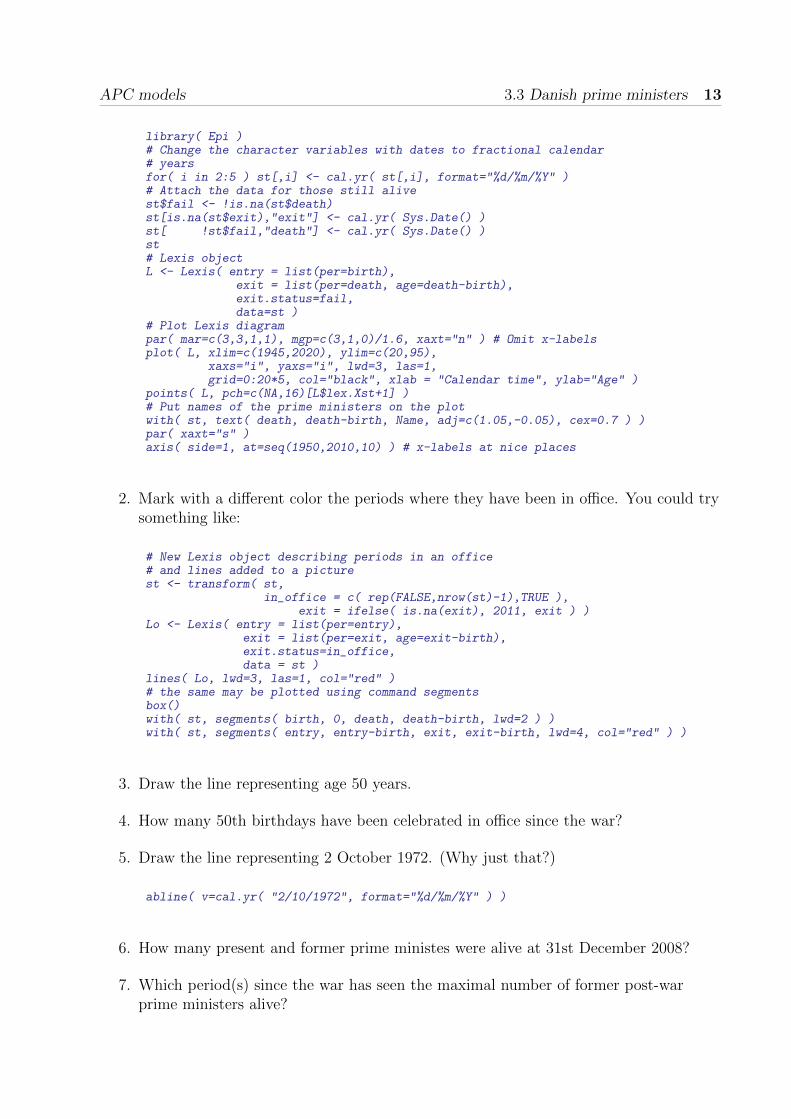
APC models 3.3 Danish prime ministers 13
library( Epi )# Change the character variables with dates to fractional calendar# yearsfor( i in 2:5 ) st[,i] <- cal.yr( st[,i], format="%d/%m/%Y" )# Attach the data for those still alivest$fail <- !is.na(st$death)st[is.na(st$exit),"exit"] <- cal.yr( Sys.Date() )st[ !st$fail,"death"] <- cal.yr( Sys.Date() )st# Lexis objectL <- Lexis( entry = list(per=birth),
exit = list(per=death, age=death-birth),exit.status=fail,data=st )
# Plot Lexis diagrampar( mar=c(3,3,1,1), mgp=c(3,1,0)/1.6, xaxt="n" ) # Omit x-labelsplot( L, xlim=c(1945,2020), ylim=c(20,95),
xaxs="i", yaxs="i", lwd=3, las=1,grid=0:20*5, col="black", xlab = "Calendar time", ylab="Age" )
points( L, pch=c(NA,16)[L$lex.Xst+1] )# Put names of the prime ministers on the plotwith( st, text( death, death-birth, Name, adj=c(1.05,-0.05), cex=0.7 ) )par( xaxt="s" )axis( side=1, at=seq(1950,2010,10) ) # x-labels at nice places
2. Mark with a different color the periods where they have been in office. You could trysomething like:
# New Lexis object describing periods in an office# and lines added to a picturest <- transform( st,
in_office = c( rep(FALSE,nrow(st)-1),TRUE ),exit = ifelse( is.na(exit), 2011, exit ) )
Lo <- Lexis( entry = list(per=entry),exit = list(per=exit, age=exit-birth),exit.status=in_office,data = st )
lines( Lo, lwd=3, las=1, col="red" )# the same may be plotted using command segmentsbox()with( st, segments( birth, 0, death, death-birth, lwd=2 ) )with( st, segments( entry, entry-birth, exit, exit-birth, lwd=4, col="red" ) )
3. Draw the line representing age 50 years.
4. How many 50th birthdays have been celebrated in office since the war?
5. Draw the line representing 2 October 1972. (Why just that?)
abline( v=cal.yr( "2/10/1972", format="%d/%m/%Y" ) )
6. How many present and former prime ministes were alive at 31st December 2008?
7. Which period(s) since the war has seen the maximal number of former post-warprime ministers alive?
14 3.4 Rates and survival APC models
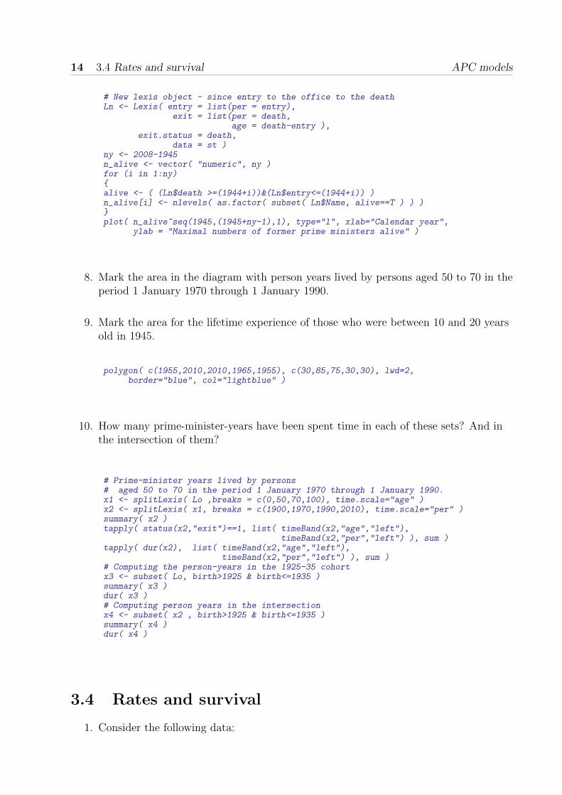
# New lexis object - since entry to the office to the deathLn <- Lexis( entry = list(per = entry),
exit = list(per = death,age = death-entry ),
exit.status = death,data = st )
ny <- 2008-1945n_alive <- vector( "numeric", ny )for (i in 1:ny){alive <- ( (Ln$death >=(1944+i))&(Ln$entry<=(1944+i)) )n_alive[i] <- nlevels( as.factor( subset( Ln$Name, alive==T ) ) )}plot( n_alive~seq(1945,(1945+ny-1),1), type="l", xlab="Calendar year",
ylab = "Maximal numbers of former prime ministers alive" )
8. Mark the area in the diagram with person years lived by persons aged 50 to 70 in theperiod 1 January 1970 through 1 January 1990.
9. Mark the area for the lifetime experience of those who were between 10 and 20 yearsold in 1945.
polygon( c(1955,2010,2010,1965,1955), c(30,85,75,30,30), lwd=2,border="blue", col="lightblue" )
10. How many prime-minister-years have been spent time in each of these sets? And inthe intersection of them?
# Prime-minister years lived by persons# aged 50 to 70 in the period 1 January 1970 through 1 January 1990.x1 <- splitLexis( Lo ,breaks = c(0,50,70,100), time.scale="age" )x2 <- splitLexis( x1, breaks = c(1900,1970,1990,2010), time.scale="per" )summary( x2 )tapply( status(x2,"exit")==1, list( timeBand(x2,"age","left"),
timeBand(x2,"per","left") ), sum )tapply( dur(x2), list( timeBand(x2,"age","left"),
timeBand(x2,"per","left") ), sum )# Computing the person-years in the 1925-35 cohortx3 <- subset( Lo, birth>1925 & birth<=1935 )summary( x3 )dur( x3 )# Computing person years in the intersectionx4 <- subset( x2 , birth>1925 & birth<=1935 )summary( x4 )dur( x4 )
3.4 Rates and survival
1. Consider the following data:
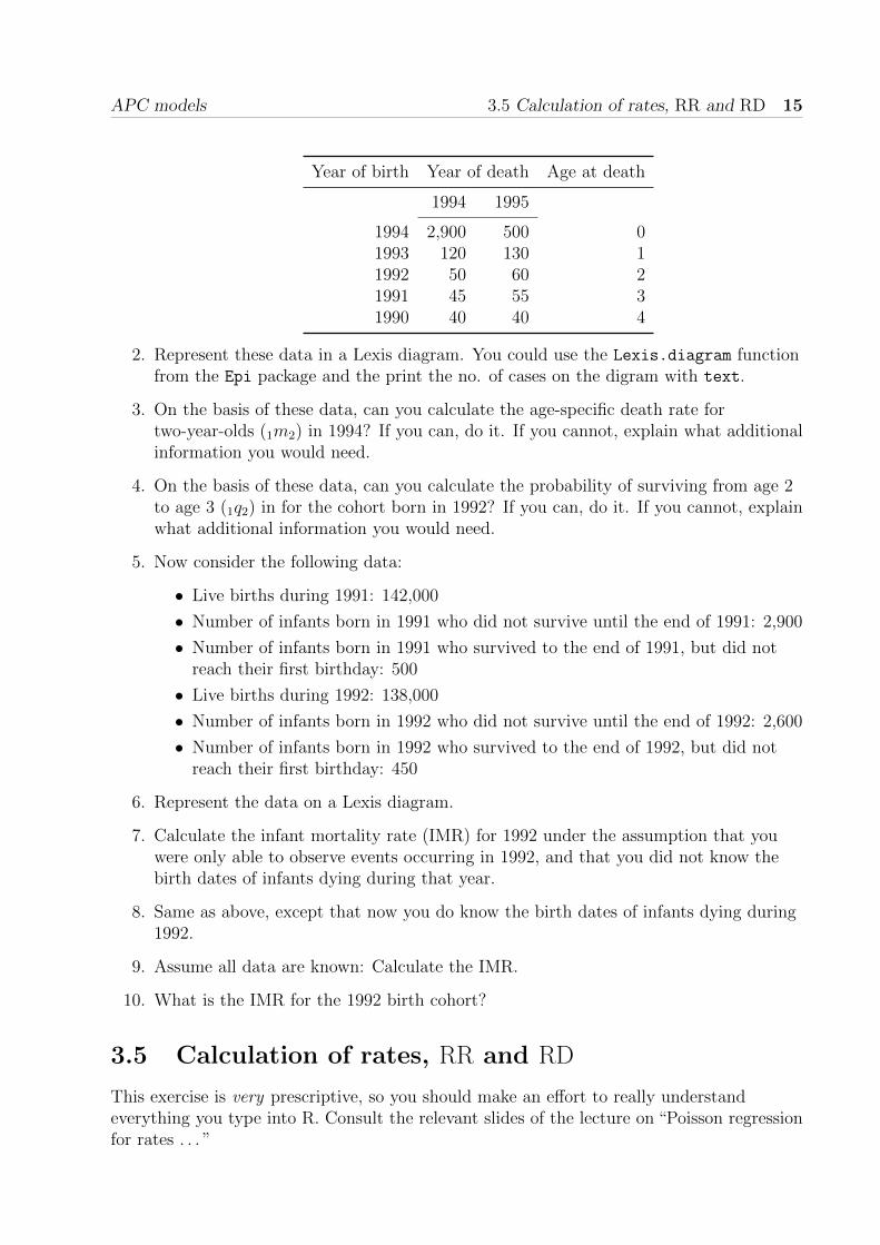
APC models 3.5 Calculation of rates, RR and RD 15
Year of birth Year of death Age at death
1994 1995
1994 2,900 500 01993 120 130 11992 50 60 21991 45 55 31990 40 40 4
2. Represent these data in a Lexis diagram. You could use the Lexis.diagram functionfrom the Epi package and the print the no. of cases on the digram with text.
3. On the basis of these data, can you calculate the age-specific death rate fortwo-year-olds (1m2) in 1994? If you can, do it. If you cannot, explain what additionalinformation you would need.
4. On the basis of these data, can you calculate the probability of surviving from age 2to age 3 (1q2) in for the cohort born in 1992? If you can, do it. If you cannot, explainwhat additional information you would need.
5. Now consider the following data:
• Live births during 1991: 142,000
• Number of infants born in 1991 who did not survive until the end of 1991: 2,900
• Number of infants born in 1991 who survived to the end of 1991, but did notreach their first birthday: 500
• Live births during 1992: 138,000
• Number of infants born in 1992 who did not survive until the end of 1992: 2,600
• Number of infants born in 1992 who survived to the end of 1992, but did notreach their first birthday: 450
6. Represent the data on a Lexis diagram.
7. Calculate the infant mortality rate (IMR) for 1992 under the assumption that youwere only able to observe events occurring in 1992, and that you did not know thebirth dates of infants dying during that year.
8. Same as above, except that now you do know the birth dates of infants dying during1992.
9. Assume all data are known: Calculate the IMR.
10. What is the IMR for the 1992 birth cohort?
3.5 Calculation of rates, RR and RD
This exercise is very prescriptive, so you should make an effort to really understandeverything you type into R. Consult the relevant slides of the lecture on “Poisson regressionfor rates . . . ”
16 3.5 Calculation of rates, RR and RD APC models
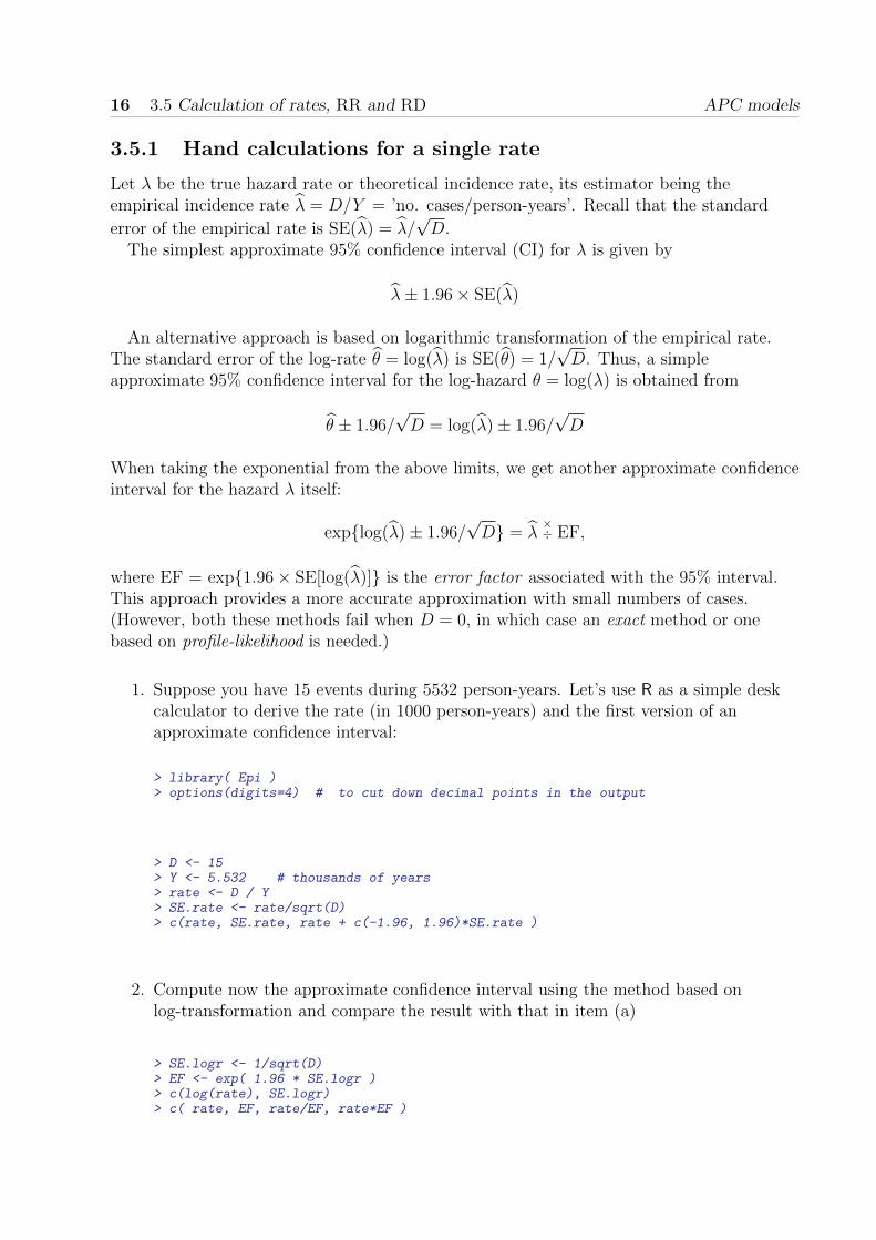
3.5.1 Hand calculations for a single rate
Let λ be the true hazard rate or theoretical incidence rate, its estimator being theempirical incidence rate λ = D/Y = ’no. cases/person-years’. Recall that the standard
error of the empirical rate is SE(λ) = λ/√D.
The simplest approximate 95% confidence interval (CI) for λ is given by
λ± 1.96× SE(λ)
An alternative approach is based on logarithmic transformation of the empirical rate.The standard error of the log-rate θ = log(λ) is SE(θ) = 1/
√D. Thus, a simple
approximate 95% confidence interval for the log-hazard θ = log(λ) is obtained from
θ ± 1.96/√D = log(λ)± 1.96/
√D
When taking the exponential from the above limits, we get another approximate confidenceinterval for the hazard λ itself:
exp{log(λ)± 1.96/√D} = λ
×÷ EF,
where EF = exp{1.96× SE[log(λ)]} is the error factor associated with the 95% interval.This approach provides a more accurate approximation with small numbers of cases.(However, both these methods fail when D = 0, in which case an exact method or onebased on profile-likelihood is needed.)
1. Suppose you have 15 events during 5532 person-years. Let’s use R as a simple deskcalculator to derive the rate (in 1000 person-years) and the first version of anapproximate confidence interval:
> library( Epi )> options(digits=4) # to cut down decimal points in the output
> D <- 15> Y <- 5.532 # thousands of years> rate <- D / Y> SE.rate <- rate/sqrt(D)> c(rate, SE.rate, rate + c(-1.96, 1.96)*SE.rate )
2. Compute now the approximate confidence interval using the method based onlog-transformation and compare the result with that in item (a)
> SE.logr <- 1/sqrt(D)> EF <- exp( 1.96 * SE.logr )> c(log(rate), SE.logr)> c( rate, EF, rate/EF, rate*EF )

APC models 3.5 Calculation of rates, RR and RD 17
3.5.2 Poisson model for a single rate with logarithmic link
You are able to estimate λ and compute its CI with a Poisson model, as described in therelevant slides in the lecture handout.
3. Use the number of events as the response and the log-person-years as an offset term,and fit the Poisson model with log-link
> m <- glm( D ~ 1, family=poisson(link=log), offset=log(Y) )> summary( m )
What is the interpretation of the parameter in this model?
4. The summary method produces too much output. You can extract CIs for the modelparameters directly from the fitted model on the scale determined by the linkfunction with the ci.lin()-function. Thus, the estimate, SE, and confidence limitsfor the log-rate θ = log(λ) are obtained by:
> ci.lin( m )
However, to get the confidence limits for the rate λ = exp(θ) on the original scale, theresults must be exp-transformed:
> ci.lin( m, Exp=T)
To get just the point estimate and CI for λ from log-transformed quantities you arerecommended to use function ci.exp(), which is actually a wrapper of ci.lin():
> ci.exp( m)> ci.lin( m, Exp=T)[, 5:7]
Both functions are found from Epi package. – Note that the test statistic andP -value are rarely interesting quantities for a single rate.
5. There is an alternative way of fitting a Poisson model: Use the empirical rateλ = D/Y as a scaled Poisson response, and the person-years as weight instead ofoffset (albeit it will give you a warning about non-integer response in a Poissonmodel, but you can ignore this warning):
> mw <- glm( D/Y ~ 1, family=poisson, weight=Y )> ci.exp( mw)
Verify that this gave the same results as above.
3.5.3 Poisson model for a single rate with identity link
The advantage of the approach based on weighting is that it allows sensible use of theidentity link. The response is the same but the parameter estimated is now the rate itself,not the log-rate.
6. Fit the Poisson model with identity link

18 3.5 Calculation of rates, RR and RD APC models
> mi <- glm( D/Y ~ 1, family=poisson(link=identity), weight=Y )> coef(mi)
What is the meaning of the intercept in this model?
Verify that you actually get the same rate estimate as before.
7. Now use ci.lin() to produce the estimate and the confidence intervals from thismodel:
> ci.lin( mi )> ci.lin( mi )[, c(1,5,6)]
3.5.4 Poisson model assuming same rate for several periods
Now, suppose the events and person years are collected over three periods.
8. Read in the data and compute period-specific rates
> Dx <- c(3,7,5)> Yx <- c(1.412,2.783,1.337)> Px <- 1:3> rates <- Dx/Yx> rates
9. Fit the same model as before, assuming a single rate to the data for the separateperiods. Compare the result from previous ones
> m3 <- glm( Dx ~ 1, family=poisson, offset=log(Yx) )> ci.exp(m3)
10. Now test whether the rates are the same in the three periods: Try to fit a model withthe period as a factor in the model:
> mp <- glm( Dx ~ factor(Px), offset=log(Yx), family=poisson )
and compare the two models using anova() with the argument test="Chisq":
> anova( m3, mp, test="Chisq" )
Compare the test statistic to the deviance of the model mp.
What is the deviance good for?
APC models 3.5 Calculation of rates, RR and RD 19
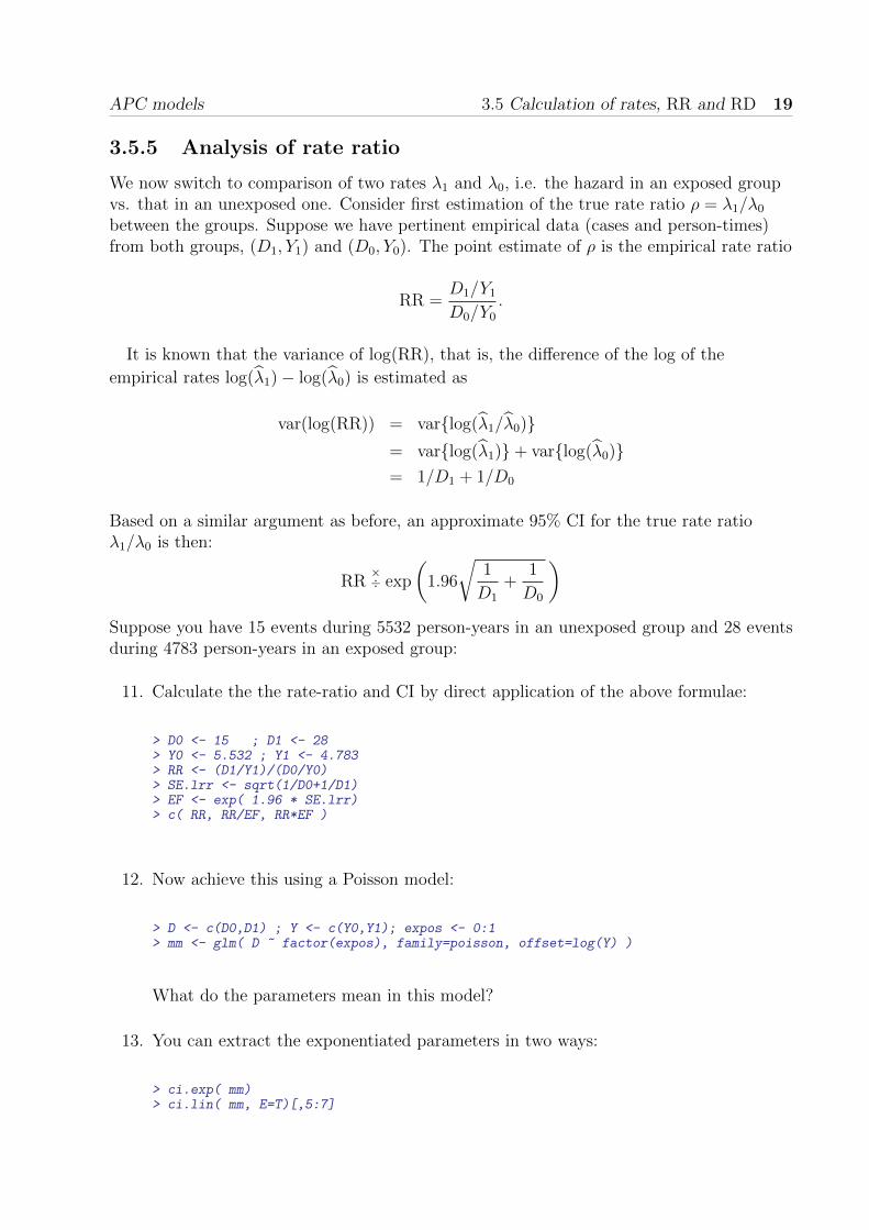
3.5.5 Analysis of rate ratio
We now switch to comparison of two rates λ1 and λ0, i.e. the hazard in an exposed groupvs. that in an unexposed one. Consider first estimation of the true rate ratio ρ = λ1/λ0
between the groups. Suppose we have pertinent empirical data (cases and person-times)from both groups, (D1, Y1) and (D0, Y0). The point estimate of ρ is the empirical rate ratio
RR =D1/Y1
D0/Y0
.
It is known that the variance of log(RR), that is, the difference of the log of the
empirical rates log(λ1)− log(λ0) is estimated as
var(log(RR)) = var{log(λ1/λ0)}= var{log(λ1)}+ var{log(λ0)}= 1/D1 + 1/D0
Based on a similar argument as before, an approximate 95% CI for the true rate ratioλ1/λ0 is then:
RR×÷ exp
(1.96
√1
D1
+1
D0
)Suppose you have 15 events during 5532 person-years in an unexposed group and 28 eventsduring 4783 person-years in an exposed group:
11. Calculate the the rate-ratio and CI by direct application of the above formulae:
> D0 <- 15 ; D1 <- 28> Y0 <- 5.532 ; Y1 <- 4.783> RR <- (D1/Y1)/(D0/Y0)> SE.lrr <- sqrt(1/D0+1/D1)> EF <- exp( 1.96 * SE.lrr)> c( RR, RR/EF, RR*EF )
12. Now achieve this using a Poisson model:
> D <- c(D0,D1) ; Y <- c(Y0,Y1); expos <- 0:1> mm <- glm( D ~ factor(expos), family=poisson, offset=log(Y) )
What do the parameters mean in this model?
13. You can extract the exponentiated parameters in two ways:
> ci.exp( mm)> ci.lin( mm, E=T)[,5:7]

20 3.5 Calculation of rates, RR and RD APC models
3.5.6 Analysis of rate difference
When estimating the true rate difference δ = λ1 − λ0, the variance of the natural estimatorRD = D1/Y1 −D0/Y0 is (since the empirical rates are based on independent samples) justthe sum of the variances:
var(RD) = var(λ1) + var(λ0)
= D1/Y2
1 +D0/Y2
0
14. Use this formula to compute the rate difference and a 95% confidence interval for it:
> rd <- diff( D/Y )> sed <- sqrt( sum( D/Y^2 ) )> c( rd, rd+c(-1,1)*1.96*sed )
15.
16. Verify that this is the confidence interval you get when you fit an additive model withexposure as factor:
> ma <- glm( D/Y ~ factor(expos),+ family=poisson(link=identity), weight=Y )> ci.lin( ma )[, c(1,5,6)]
3.5.7 Calculations using matrix tools
NB. This subsection requires some familiarity with matrix algebra.
17. You can explore the function ci.mat(), which lets you use matrix multiplication(operator '%*%' in R) to produce confidence interval from an estimate and itsstandard error (or CIs from whole columns of estimates and SEs):
> ci.mat> ci.mat()
Apply this to the single rate calculations in 1.6.1:
> c( rate, SE.rate ) %*% ci.mat()> exp( c( log(rate), SE.logr ) %*% ci.mat() )
18. For computing the rate ratio and its CI as in 1.6.5, matrix multiplication withci.mat() should give the same result as there:
> exp( c( log(RR), SE.lrr ) %*% ci.mat() )
19. Look again the model used to analyse the rate ratio in 1.6.5(b). Often one would liketo get simultaneously both the rates and the ratio between them. This can beachieved in one go using the contrast matrix argument ctr.mat to ci.lin() orci.exp(). Try:
APC models 3.6 Estimation and reporting of linear and curved effects 21
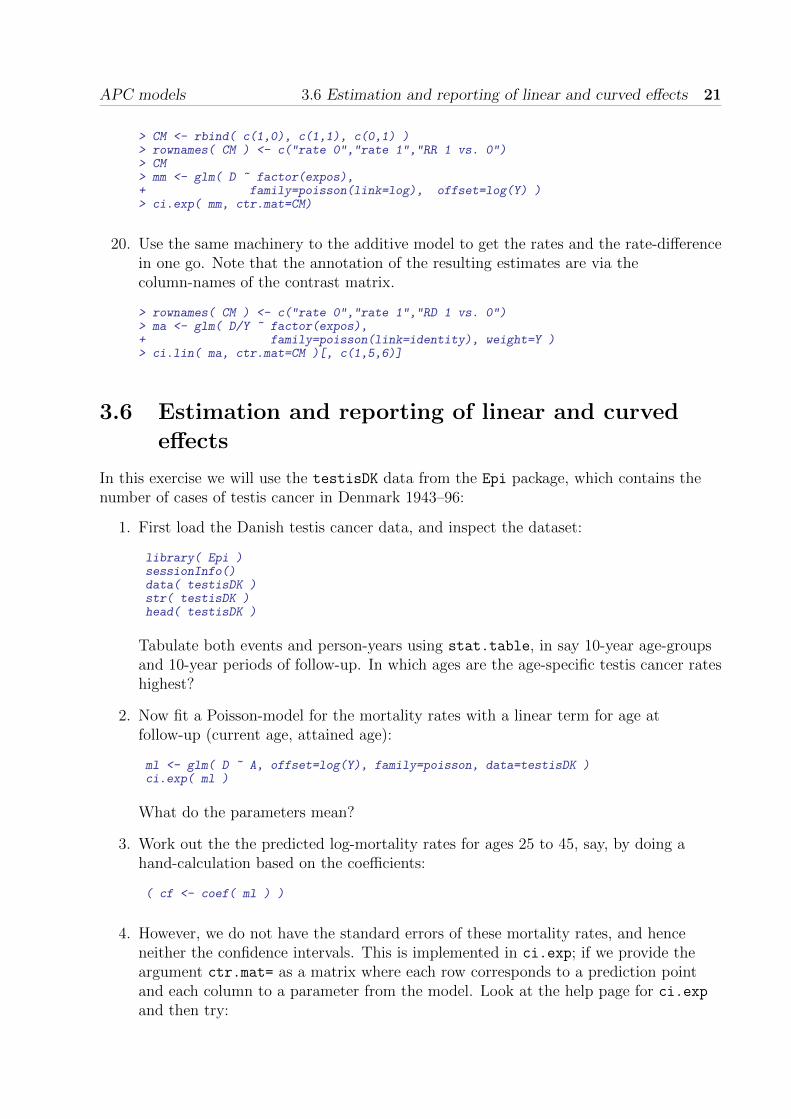
> CM <- rbind( c(1,0), c(1,1), c(0,1) )> rownames( CM ) <- c("rate 0","rate 1","RR 1 vs. 0")> CM> mm <- glm( D ~ factor(expos),+ family=poisson(link=log), offset=log(Y) )> ci.exp( mm, ctr.mat=CM)
20. Use the same machinery to the additive model to get the rates and the rate-differencein one go. Note that the annotation of the resulting estimates are via thecolumn-names of the contrast matrix.
> rownames( CM ) <- c("rate 0","rate 1","RD 1 vs. 0")> ma <- glm( D/Y ~ factor(expos),+ family=poisson(link=identity), weight=Y )> ci.lin( ma, ctr.mat=CM )[, c(1,5,6)]
3.6 Estimation and reporting of linear and curved
effects
In this exercise we will use the testisDK data from the Epi package, which contains thenumber of cases of testis cancer in Denmark 1943–96:
1. First load the Danish testis cancer data, and inspect the dataset:
library( Epi )sessionInfo()data( testisDK )str( testisDK )head( testisDK )
Tabulate both events and person-years using stat.table, in say 10-year age-groupsand 10-year periods of follow-up. In which ages are the age-specific testis cancer rateshighest?
2. Now fit a Poisson-model for the mortality rates with a linear term for age atfollow-up (current age, attained age):
ml <- glm( D ~ A, offset=log(Y), family=poisson, data=testisDK )ci.exp( ml )
What do the parameters mean?
3. Work out the the predicted log-mortality rates for ages 25 to 45, say, by doing ahand-calculation based on the coefficients:
( cf <- coef( ml ) )
4. However, we do not have the standard errors of these mortality rates, and henceneither the confidence intervals. This is implemented in ci.exp; if we provide theargument ctr.mat= as a matrix where each row corresponds to a prediction pointand each column to a parameter from the model. Look at the help page for ci.expand then try:

22 3.6 Estimation and reporting of linear and curved effects APC models
( CM <- cbind( 1, 25:45 ) )round( ci.exp( ml, ctr.mat=CM )*10^5, 3 )
5. Use this machinery to derive and plot the mortality rates over the range from 15 to65 years, say:
C1 <- cbind( 1, 15:65 )matplot( 15:65, ci.exp( ml, ctr.mat=C1 )*10^5,
log="y", xlab="Age", ylab="Testis cancer incidence rate per 100,000 PY",type="l", lty=1, lwd=c(3,1,1), col="black" )
6. Now check if the mortality rates really are eksponentially increasing by age (that islinearly on the log-scale), by adding a quadratic term to the model. Note that youmust use the expression I(A^2) in the modelleing in order to avoid that the “^” isinterpreted as part of the model formula:
mq <- glm( D ~ A + I(A^2), offset=log(Y), family=poisson, data=testisDK )ci.exp( mq, Exp=F )
Then plot the estimated rates under the quadratic model.
aa <- 15:65C2 <- cbind( 1, aa, aa^2 )matplot( aa, ci.exp( mq, ctr.mat=C2 )*10^5,
log="y", xlab="Age", ylab="Testis cancer incidence rate per 100,000 PY",type="l", lty=1, lwd=c(3,1,1), col="black" )
Try to overlay the estimated rates from the model with linear efect of age — you willneed the function matlines.
7. Repeat the same using a 3rd degree polynomial.
8. Instead of continuing with higher powers of age we could use fractions of powers, orwe could use splines, piecevise polynomial curves, that fit nicely together at joinpoints (knots). This is implemented in the splines package, in the function ns,which returns a matrix. There is a wrapper Ns in the Epi-package that automaticallydesignate the smallest and largest knots a boundary knots, beyond which the resultingcurve is linear:
library( splines )ms <- glm( D ~ Ns(A,knots=seq(15,65,10)), offset=log(Y),
family=poisson, data=testisDK )
In order to extract the estimated effects, construct a contrast matrix that correspondto the parameters of the model:
As <- Ns( aa, knots=seq(15,65,10) )matplot( aa, ci.exp( ms, ctr.mat=cbind(1,As) )*10^5,
log="y", xlab="Age", ylab="Testis cancer incidence rate per 100,000 PY",type="l", lty=1, lwd=c(3,1,1), col="black" )
9. Now add a linear term in calendar time P to the model, and make a prediction of theincidence rates in 1970, say:
APC models 3.6 Estimation and reporting of linear and curved effects 23
msp <- glm( D ~ Ns(A,knots=seq(15,65,10)) + P, offset=log(Y), family=poisson, data=testisDK )matplot( aa, ci.exp( msp, ctr.mat=cbind(1,As,1970) )*10^5,
log="y", xlab="Age", ylab="Testis cancer incidence rate per 100,000 PY",type="l", lty=1, lwd=c(3,1,1), col="black" )
Note that cbind automatically will expand the 1 and the 1970 to match the numberof rows of As.
10. Extract the RR relative to 1970, by using the subset argument to ci.exp:
ci.exp( msp, subset="P" )
What is the annual relative increase in the testis cancer incidence rates? Show theRR of testis cancer by year relative to 1970 by multipling the log-RR for period withthe distance form 1970, such as:
yy <- 1943:1996Cp1 <- cbind( yy - 1970 )matplot( yy, ci.exp( msp, ctr.mat=Cp1, subset="P" ),
log="y", xlab="Date", ylab="RR of Testis cancer",type="l", lty=1, lwd=c(3,1,1), col="black" )
abline( h=1 )
11. Try to add a quadratic term to the period effect, and plot the resulting RR relativeto 1970.Hint: In order to extract the quadratic effects relative to 1970, you must form thematrix of linear and quadratic period, and a corresponding matrix where all rows areidentical to the 1970 row:
msp <- glm( D ~ Ns(A,knots=seq(15,65,10)) + P + I(P^2),offset=log(Y), family=poisson, data=testisDK )
Cq <- cbind( yy, yy^2 ) - cbind( rep(1970,length(yy)), 1970^2 )
Use this matrix as arguent to ci.exp
12. Now investigate if there is any non-linearity in period beyond the quadratic, byfitting fit a spline for (P) as well, and comparing the models. Plot the resulting RRby year, relative to 1970 too. You must define a contrast matrix corresponding to theyears where the prediction is made, as well as a matrix with the same number ofrows, but with all rows identical to the one corresponding to the reference year. Youmust use the differenec of these two as the arument to ctr.mat in ci.exp.
13. Plot the estimated age-specific rates in 1970 from this model. Note that you need areference matrix for the period with all rows identical to the 1970 row, but this timewith the same number of rows as the age-prediciton points.
14. Collect these steps in a general outline, where you first define the knots, and thepoints of age and period prediction, and then fit the model and do the two plots.
15. Form a new variable in the data frame, B=P-A, the data of birth, and repeat the lastanalysis with this variable instead of P.

24 3.7 Age-period model APC models
3.7 Age-period model
The following exercise is aimed at familiarizing you with the parametrization of theage-period model. It will give you the opportunity explore how to extract and and plotparameter estimates from models. It is based on Danish male lung cancer incidence data in5-year classes.
1. Read the data in the file lung5-M.txt as in the tabulation exercise:
lung <- read.table( "../data/lung5-M.txt", header=T )lungwith( lung , table( A ) )with( lung , table( P ) )with( lung , tapply( Y, list(A,P), sum ) )
What do these tables show?
2. Fit a Poisson model with effects of age (A) and period (P) as class variables:
ap.1 <- glm( D ~ factor(A) + factor(P) + offset(log(Y)),family=poisson, data=lung )
summary( ap.1 )
What do the parameters refer to, i.e. which ones are log-rates and which ones arerate-ratios?
3. Fit the same model without intercept (use -1 in the model formula); call it ap.0 —we shall refer to this subsequently. What do the parameters now refer to?
4. Fit the same model, using the period 1968–72 as the reference period, by using therelevel command for factors to make 1968 the first level:
ap.3 <- glm( D ~ factor(A) - 1 + relevel(factor(P),"1968") + offset(log(Y)),family=poisson, data=lung )
5. Extract the prameters from the model, by doing:
ap.cf <- summary( ap.3 )$coef
6. Now plot the estimated age-specific incidence rates, remembering to annoatte them withthe correct scale. We need the first 10 parameters, with their standard errors:
age.cf <- ap.cf[1:10,1:2]
This means that we take rows 1–10 and columns 1–2. The corresponding age classes are40, . . . , 85. The midpoints of these age-classes are 2.5 years higher. The ages can begenerated in R by saying seq(40,85,5)+2.5.
Now put confidence limits on the curves by taking ±1.96× s.e.. The line of the estimatescan be over-drawn once more in a thicker style:
lines( seq(40,85,5)+2.5, exp(age.cf[,1]), lwd=3 )

APC models 3.7 Age-period model 25
7. Now for the rate-ratio-parameters, take the rest of the coefficients:
RR.cf <- ap.cf[11:20,1:2]
But the reference group is missing, so we must stick two 0s in the correct place. We use thecommand rbind (row-bind):
RR.cf <- rbind( RR.cf[1:5,], c(0,0), RR.cf[6:10,] )
Now we have the same situation as for the age-specific rates, and can plot the relative risks(relative to 1968) in precisely the same way as for the agespecific rates.
Make a line-plot of the relative risks with confidence intervals.
8. However, the relevant parameters may also be extracted directly from the model withoutintercept, using the function ci.lin (remember to read the documentation for this!)
The point is to define a contrast matrix, which multiplied to (a subset of) the parametersgives the rates in the reference period. The log-rates in the reference period (the first levelof factor(P) are the age-parameters. The log-rates in the period labelled 1968 are theseplus the period estimate from 1968.
Now construct the following matrix and look at it:
cm.A <- cbind( diag( nlevels( factor(lung$A) ) ), 1 )
Now look at the parameters extracted by ci.lin, using the subset= argument:
ci.lin( ap.0, subset=c("A","1968") )
Now use the argument ctr.mat= in ci.lin to produce the rates in period 1968 and plotthem on a log-scale.
9. Save the estimates of age aned period effects along with the age-points and period-points,using save (look up the help page if you are not familiar with it. You will need these in thenext exercise on the age-cohort model.
10. We can also use the same machinery to extract the rate-ratios relative to 1968. Thecontrast matrix to use is the difference between two: The first one is the one that extractsthe rate-ratios with a prefixed 0:
cm.P <- rbind(0,diag( nlevels(factor(lung$P))-1 ) )cm.Pci.lin( ap.0, subset="P", ctr.mat=cm.P )
In order to subtract the value corresponding to 1968, we must subtract a 11× 10 matrix,that just selects the 1968 column:
cm.Pref <- cm.P * 0cm.Pref[,5] <- 1cm.Pref
The contrast matrix to use is the difference between these two:
cm.P - cm.Prefci.lin( ap.0, subset="P", ctr.mat=cm.P-cm.Pref )

26 3.8 Age-cohort model APC models
Use the Exp=TRUE argument to get the rate-ratios and plot these with confidence intervalson a log-scale.
11. For the real nerds: Plot the rates and the rate ratios beside each other, and make sure thatthe physical extent of the units on both the x-axis and the y-axis are the same.
Hint: You may want to use par(mar=c(0,0,0,0), oma=), the function layout as well asthe xaxs="i" argument to plot.
3.8 Age-cohort model
This exercise is aimed at familiarizing you with the parametrization of the age-cohortmodel. It will give you the opportunity explore how to extract and and plot parameterestimates from models. It is parallel to the exercise on the age-period model and is thereforless detailed.
1. Read the data in the file lung5-M.txt as in the tabulation exercise:
library(Epi)lung <- read.table( "../data/lung5-M.txt", header=T )lungattach( lung )table( A )table( P )table( P-A )
What do these tables show?
2. Fit a Poisson model with effects of age (A) and cohort (C) as class variables. Youwill need to form the variable C (cohort) as P − A first.
What do the parameters refer to ?
3. Fit the same model without intercept. What do the parameters now refer to ?
Hint: Use -1 in the model formula.
4. Fit the same model, using the cohort 1908 as the reference cohort. What do theparameters represent now?
Hint: Use the Relevel command for factors to make 1968 the first level.
5. What is the range of birth dates represented in the cohort 1908?
6. Extract the age-specific incidence parameters from the model and plot then againstage. Remember to annotate them with the correct units. Add 95% confidenceintervals.
Hint: Use the function ci.lin from the Epi package.
7. Extract the cohort-specific rate-ratio parameters and plot then against the date ofbirth (cohort). Add 95% confidence intervals.
8. Now load the estimates from the age-period model, and plot the estimatedage-specific rates from the two models on top of each other.
Why are they different? In particular, why do they have different slopes?

APC models 3.9 Age-drift model 27
3.9 Age-drift model
This exercise is aimed at introducing the age-drift model and make you familiar with thetwo different ways of parametrizing this model. Like the two previous exercises it is basedon the male lung cancer data.
1. First read the data in the file lung5-M.txt and create the cohort variable:
lung <- read.table( "../data/lung5-M.txt", header=T )lung$C <- lung$P - lung$A
Alternatively you can do:
lung <- transform( lung, C = P - A )
2. Fit a Poisson model with effects of age as class variable and period P as continuousvariable.
What do the parameters refer to ?
3. Fit the same model without intercept. What do the parameters now refer to?
4. Fit the same model, using the period 1968–72 as the reference period.
Hint: When you center a variable on a reference value ref, say, by entering P-ref
directly in the model formula will cause a crash, because the “-” is interpreted as amodel operator. You must “hide” the minus from the model formula interpretation byusing the identity function, i.e. use: I(P-ref).
Now what do the parameters represent?
5. Fit a model with cohort as a continuous variable, using 1908 as the reference, andwithout intercept. What do the resulting parameters represent?
6. Compare the deviances and the slope estimates from the models with cohort driftand period drift.
7. What is the relationship between the estimated age-effects in the two models?
Verify this empirically by converting one set of age-parameters to the other.
8. Plot the age-specific incidence rates from the two different models in the same panel.
9. The rates from the model are:
log(λap) = αp + δ(p− 1970.5)
Therefore, with an x-variable: (1943,. . . ,1993) + 2.5, the log rate ratio relative to1970.5 will be:
log RR = δ × xand the upper and lower confidence bands:
log RR = (δ ± 1.96× s.e.(δ))× x
Now extract the slope parameter, and plot the rate-ratio functions as a function ofperiod.

28 3.10 Age-period-cohort model APC models
3.10 Age-period-cohort model
The following exercise is aimed at familiarizing you with the parametrization of theage-period-cohort model and with the realtionship of the APC-model to the other modelthat you have been working with, so we will refer back to those, and assume that you havethe results from them at hand.
1. Read the data in the file lung5-M.txt as in the tabulation exercise:
lung <- read.table( "../data/lung5-M.txt", header=T )lungattach( lung )
2. Fit a Poisson model with effects of age (A), period (P) and cohort (C) as classvariables. Also fit a model with age alone as a class variable. Write down a schemeshowing the deviances and degrees of freedom for the 5 models you have models fittedto this dataset.
3. Compare the models that can be compared, with likelihood-ratio tetsts. You willwant to use anova (or specifically anova.glm) with the argument test="Chisq".
4. Next, fit the same model without intercept, and with the first and last periodparameters and the 1908 cohort parameter set to 0. Before you do so a few practicalthings must be fixed:
You can merge the first and the last period level using the Relevel function (look atthe documentation for it).
lung$Pr <- Relevel( factor(lung$P), list("first-last"=c("1943","1993") ) )
You can also use this function to make the 1908 cohort the first level of the cohortfactor:
lung$Cr <- Relevel( factor(lung$P-lung$A), "1908" )
It is a good idea to tabulate the new factor against the old one (i.e. that variablefrom which it was created) in order to meake sure that the relevelling actually is asyou intended it to be.
5. Now you can fit the model, using the factors you just defined. What do theparameters now refer to?
6. Make a graph of the parameters. Remember to take the exponential to convert theage-parameters to rates (and find out what the units are) and the period and cohortparameters to rate ratios. Also use a log-scale for the y-axis. You may want to useci.lin to facilitate this.
7. Fit the same model, using the period 1968–72 as the reference period and two cohortsof your choice as references. To decide which of the cohorts to alias it may be usefulto see how many observations there are in each:

APC models 3.11 Age-period-cohort model for Lexis triangles 29
with( lung, table(P-A) )with( lung, tapply(D,list(P-A),sum) )
Having fitted the model, now what do the parameters in it represent?
8. Make a plot of these parameters.
Add the parameters from the previous parametrization to the same graph.
3.11 Age-period-cohort model for Lexis triangles
The following exercise is aimed at showing the problems associated with age-period-cohortmodelling for triangular data.
Also you will learn how to overcome these problems by parametric modelling of the threeeffects.
1. Read the Danish male lung cancer data tabulated by age period and birth cohort,lung5-Mc.txt. List the first few lines of the dataset and make sure you understandwhat the variables refer to. Also define nthe synthetic cohorts as P5-A5:
library( Epi )ltri <- read.table( "../data/lung5-Mc.txt", header=T )ltri$S5 <- ltri$P5 - ltri$A5attach( ltri )
2. Make a Lexis diagram showing the subdivision of the follow-data. You will explorethe function Lexis.diagram.
Lexis.diagram( age=c(40,90), date=c(1943,1998), coh.grid=TRUE )
3. Use the variables A5 and P5 to fit a traditional age-period-cohort model withsynthetic cohort defined above as S5=P5-A5:
ms <- glm( D ~ -1 + factor(A5) + factor(P5) + factor(S5) + offset(log(Y)),family=poisson, data=ltri )
How many parameters does this model have? (Use the summary() function)
4. Now try to fit the model with the “real” cohort variable C5:
mc <- glm( D ~ -1 + factor(A5) + factor(P5) + factor(C5) + offset(log(Y)),family=poisson, data=ltri )
summary( mc )$df
How many parameters does this model have?
5. Plot the parameter estimates from the two models on top of each other, withconfidence intervals. Remember to put the correct scales on the plot.

30 3.11 Age-period-cohort model for Lexis triangles APC models
par( mfrow=c(1,3) )a.pt <- as.numeric( levels(factor(A5)) )p.pt <- as.numeric( levels(factor(P5)) )s.pt <- as.numeric( levels(factor(S5)) )c.pt <- as.numeric( levels(factor(C5)) )matplot( a.pt, ci.lin( ms, subset="A5", Exp=TRUE )[,5:7]/10^5,
type="l", lty=1, lwd=c(3,1,1), col="black",xlab="Age", ylab="Rates", log="y" )
matlines( a.pt, ci.lin( mc, subset="A5", Exp=TRUE )[,5:7]/10^5,type="l", lty=1, lwd=c(3,1,1), col="blue" )
matplot( p.pt, rbind( c(1,1,1), ci.lin( ms, subset="P5",Exp=TRUE )[,5:7] ),type="l", lty=1, lwd=c(3,1,1), col="black",xlab="Period", ylab="RR", log="y" )
matlines( p.pt, rbind( c(1,1,1), ci.lin( mc, subset="P5",Exp=TRUE )[,5:7] ),type="l", lty=1, lwd=c(3,1,1), col="blue" )
matplot( s.pt, rbind(c(1,1,1),ci.lin( ms, subset="S5", Exp=TRUE )[,5:7]),type="l", lty=1, lwd=c(3,1,1), col="black",xlab="Cohort", ylab="RR", log="y" )
matlines( c.pt, rbind(c(1,1,1),ci.lin( mc, subset="C5", Exp=TRUE )[,5:7]),type="l", lty=1, lwd=c(3,1,1), col="blue" )
How do the confidence limits compare between the three effects?
6. Now fit the model using the proper midpoints of the triangles as factor levels. Howmany parameters does this model have?
mt <- glm( D ~ -1 + factor(Ax) + factor(Px) + factor(Cx) + offset(log(Y)),family=poisson, data=ltri )
summary( mt )$df
7. Plot the parameters from this model in three panels as for the previous two models.
par( mfrow=c(1,3) )a.pt <- as.numeric( levels(factor(Ax)) )p.pt <- as.numeric( levels(factor(Px)) )c.pt <- as.numeric( levels(factor(Cx)) )matplot( a.pt, ci.lin( mt, subset="Ax", Exp=TRUE )[,5:7]/10^5,
type="l", lty=1, lwd=c(3,1,1), col="black",xlab="Age", ylab="Rates", log="y" )
matplot( p.pt, rbind( c(1,1,1), ci.lin( mt, subset="Px",Exp=TRUE )[,5:7] ),type="l", lty=1, lwd=c(3,1,1), col="black",xlab="Period", ylab="RR", log="y" )
matplot( c.pt, rbind(c(1,1,1),ci.lin( mt, subset="Cx", Exp=TRUE )[,5:7]),type="l", lty=1, lwd=c(3,1,1), col="black",xlab="Cohort", ylab="RR", log="y" )
We see that the parameters clearly do not convey a reasonable picture of the effects;som severe indeterminacy has crept in.
8. What is the residual deviance of this model?
summary( mt )$deviance
9. The dataset also has a variable up, which indicates whether the observation comesfrom an upper or lower triangle. Try to tabulate this variable against P5-A5-C5.
table( up, P5-A5-C5 )

APC models 3.11 Age-period-cohort model for Lexis triangles 31
10. Fit an age-period cohort model separately for the subset of the dataset from theupper triangles and from the lowere triangles. What is the residual deviance fromeach of these models and what is the sum of these. Compare to the model using theproper midpoints as factor levels.
m.up <- glm( D ~ -1 + factor(A5) + factor(P5) + factor(S5) + offset(log(Y)),family=poisson, data=subset(ltri,up==1) )
summary( m.up )$deviancem.lo <- glm( D ~ -1 + factor(A5) + factor(P5) + factor(S5) + offset(log(Y)),
family=poisson, data=subset(ltri,up==0) )summary( m.lo )$deviancesummary( m.lo )$deviance + summary( m.up )$deviancesummary( mt )$deviance
11. Next, repeat the plots of the parameters from the model using the proper midpointsas factor levels, but now super-posing the estimates (in different color) from each ofthe two models just fitted. What goes on?
par( mfrow=c(1,3) )a.pt <- as.numeric( levels(factor(Ax)) )p.pt <- as.numeric( levels(factor(Px)) )c.pt <- as.numeric( levels(factor(Cx)) )a5.pt <- as.numeric( levels(factor(A5)) )p5.pt <- as.numeric( levels(factor(P5)) )s5.pt <- as.numeric( levels(factor(S5)) )matplot( a.pt, ci.lin( mt, subset="Ax", Exp=TRUE )[,5:7]/10^5,
type="l", lty=1, lwd=c(2,1,1), col=gray(0.7),xlab="Age", ylab="Rates", log="y" )
matpoints( a5.pt, ci.lin( m.up, subset="A5", Exp=TRUE )[,5:7]/10^5,pch=c(16,3,3), col="blue" )
matpoints( a5.pt, ci.lin( m.lo, subset="A5", Exp=TRUE )[,5:7]/10^5,pch=c(16,3,3), col="red" )
matplot( p.pt, rbind( c(1,1,1), ci.lin( mt, subset="Px",Exp=TRUE )[,5:7] ),type="l", lty=1, lwd=c(2,1,1), col=gray(0.7),xlab="Period", ylab="RR", log="y" )
matpoints( p5.pt[-1], ci.lin( m.up, subset="P5", Exp=TRUE )[,5:7],pch=c(16,3,3), col="blue" )
matpoints( p5.pt[-1], ci.lin( m.lo, subset="P5", Exp=TRUE )[,5:7],pch=c(16,3,3), col="red" )
matplot( c.pt, rbind(c(1,1,1),ci.lin( mt, subset="Cx", Exp=TRUE )[,5:7]),type="l", lty=1, lwd=c(2,1,1), col=gray(0.7),xlab="Cohort", ylab="RR", log="y" )
matpoints( s5.pt[-1], ci.lin( m.up, subset="S5", Exp=TRUE )[,5:7],pch=c(16,3,3), col="blue" )
matpoints( s5.pt[-1], ci.lin( m.lo, subset="S5", Exp=TRUE )[,5:7],pch=c(16,3,3), col="red" )
12. Now, load the splines package and fit a model using the correct midpoints of thetriangles as quantitative variables in restricted cubic splines, using the function ns:
library( splines )mspl <- glm( D ~ -1 + ns(Ax,df=7,intercept=T)
+ ns(Px,df=6,intercept=F)+ ns(Cx,df=6,intercept=F) + offset(log(Y)),
family=poisson, data=ltri )
13. Compute the residual degrees of freedom for the two models and compare thedeviance of the models with these

32 3.12 Using apc.fit etc. APC models
summary( mspl )summary( mt )$deviance - summary( mspl )$deviancesummary( mt )$df - summary( mspl )$df
How do the deviances compare?
14. Make a prediction of the terms, using predict.glm using the argumenttype="terms", and plot these estimated terms.
15. Repeat the last three questions based on a moedl where you have interchanged thesequence of the period and cohort term.
3.12 Using apc.fit etc.
This exercise is aimed at introducing the functions for fitting and plotting the results fromage-period-cohort models: apc.fit apc.plot apc.lines and apc.frame.
You should read the help page for the apc.fit function, in particular you should beaware of the meaning of the argument
1. Read the testis cancer data and collapse the cases over the histological subtypes:
th <- read.table( "../data/testis-hist.txt", header=T )str( th )
Knowing the names of the variables in the dataset, you can collapse the dataset overthe histological subtypes. You may want to use the function aggregate; note thatthere is no need to tabulate by cohort, because even for the triangular data therelationship c = p− a holds.
Note that the original data had three subtypes of testis cancer, so while it is OK tosum the number of cases (D), risk time should not be aggregated across histologicalsubtypes — the aggregation is basically as for competing risks only events are addedup, the risk time is the same. (Take a look at the help page for aggregate):
2. Present the rates in 5-year age and period classes from age 15 to age 59 usingrateplot. Consider the function subset. To this end you must make a table, forexample using something like:
with( tc, tapply( D, list(floor(A/5)*5+2.5,floor((P-1943)/5)*5+1945.5), sum ) )
— assuming your aggregated data is in the data frame tc. and a similar constructionfor the risk time.
3. Fit an age-period-cohort model to the data using the machinery implemented inapc.fit. The function returns a fitted model and a parametrization, hence you mustchoose how to parametrize it, in this case "ACP" with all the drift included in thecohort effect and the reference cohort being 1918.
tapc <- apc.fit( subset( tc, A>15 & A<60 ), npar=c(10,10,10), parm="ACP", ref.c=1918 )
Can any of the effects be omitted from the model?

APC models 3.13 Statin use in the Netherlands 33
4. Plot the estimates using the apc.plot function:
apc.plot( tapc, ci=TRUE )
5. Now explore in more depth the cohort effect by increasing the number of parametersused for it:
tapc <- apc.fit( subset( tc, A>15 & A<60 ), npar=c(10,10,20),parm="ACP", ref.c=1918, scale=10^5 )
fp <- apc.plot( tapc, ci=TRUE )
Do the extra parameters for the cohort effect have any influence on the model fit?
6. Explore the effect of using the residual method instead, and over-plot the estimatesfrom this method on the existing plot:
7. The standard display is not very pretty — it gives an overview, but certainly notanything worth publishing, hence a bit of handwork is needed. Use the apc.frame forthis, and create a nicer plot of the estimates from the residual model. You may notagree with all the parameters suggested here:
par( mar=c(3,4,1,4), mgp=c(3,1,0)/1.7, las=1 )fp <- apc.frame( a.lab=seq(20,60,10),
a.tic=seq(10,60,5),cp.lab=seq(1900,2000,20),cp.tic=seq(1885,2000,5),r.lab=c(c(1,2,5)/10,1,2,5,10),r.tic=c(1:9/10,1:10),gap=8,
rr.ref=1)apc.lines( tapc, ci=TRUE, col="blue", frame.par=fp )apc.lines( tac.p, ci=TRUE, col="red", frame.par=fp )
8. Try to repeat the exercise using period as the primary timescale, and add this to theplot as well.
What is revealed by looking at the data this way?
3.13 Statin use in the Netherlands
Bijlsma et al. published an analysis of the prevalence of statin use in the Netherlands [5],available as http://bendixcarstensen.com/APC/MPIDR-2016/Bijlsma.2012.pdf. Theauthors have kindly put the data at our disposal, so this exercise is partly replicating theanalysis in the paper, partly assessing how variants of the model behave.
1. Start by reading the data from the paper — slightly modified so that A and P noware coded as quantitative variables corresponding to the mean in each subset of theLexis diagram:
statin <- read.csv( "../data/statin.csv" )str( statin )head( statin )
34 3.14 Lung cancer in Danish women APC models
2. Now fit AP and APC models as described in the paper. In order to fix cohort effectsto be 0 for specific cohorts you will need to explore the levels of factor(P-A) andsubsequently use the function Relevel to merge the two levels to the first.
Make sure you know where the overall prevalence rates goes (with the age-effectperhaps?)
3. Then try to fit a model with suitable smooth terms in age, period and cohort, usingfor example apc.fit. Are the conclusions substantially different with respect to theperiod and cohort effects?
4. The outcome variable (D) is the number of persons that in a given period (calendaryear) take out at least one prescription of statins, and the exposure Y is the averagenumber of persons in the period. One might then argue that the outcome were bettermodeled as a fraction and not a rate; that is with a binomial distribution of D out ofY persons.
Try the same sequence of models as before and check if similar conclusion emergewhen using logit link, log link and complementary log−log link (available asargument to the binomial family argument).
5. Finally check if any of the Lee-Carter models provide viable alternatives to theAPC-models.
3.14 Lung cancer in Danish women
This exercise is parallel to the example on male lung cancer from the lectures. The point isto fit age-period-cohort models as well as Lee-Carter models and inspect their relativemerits and different fits to data on female lung cancer in Denmark.
1. Read the lung cancer data from the file lung-md.txt from the data repository, andsubset to women only (sex==2), and inspect no. of cases per 5-year age-class:
library( Epi )lC <- read.table( "../data/lung-mf.txt", header=TRUE )lF <- subset( lC, sex==2 )
2. Use xtabs to get an overview of cases and incidence rates (per 1000 PY, say), andderive the rates for use with the function rateplot.
3. When fitting APC-models and Lee-Carter models we shall use natural splines forfitting, so we must devise knots on the age and time-scales for the splines. Since theinformtion in the data on event rates is in the number of cases, we would like to placethe n knots such that there is 1/n between each pair of successive knots and 1/2nbelow the first and obove the last knot. Now use the quantile function for this,using for example (we do not necessarily want 8 knots):
quantile( rep( A,D), probs=(1:8-0.5)/8 )

APC models 3.15 Histological subtypes of testis cancer 35
4. Use apc.fit to fit an APC-model to data using the chosen knots. You mustcontemplate the type of parametrization and possible reference points on the peridoand cohort scales — read the help page for apc.fit.
5. Plot the estimated effects uisng plot.apc and possible apc.frame for increasedcontrol of the plot.
6. For comparison with the APC-model, fit the two Lee-Carter models, one withage-period and one with age-cohort interaction, and compare the fit of these modelswith the fit of the APC-model. You should use the LCa.fit function from the Epi
package. In order that models be comparable, you must use the same knots for age,period and cohort effects. Alternatively the lca.rh function from the ilc package.
7. Plot the estimated components of the Lee-Carter models.
8. (This exercise is quite long-winded). In order to get a better view of the behaviour ofthe different models, plot the predicted rates from the two Lee-Carter models overthe time-span of the data frame at select ages (say 50, 60, 70 and 80), using bothperiod and cohort as time-axis. Compare with the fits from the AP, AC andAPC-models. Make similar plots of the predicted age-specific rates for select periodand cohorts, and again compare the 5 different model fits.
3.15 Histological subtypes of testis cancer
The purpose of this exercise is to handle two different rates that both obey (possiblydifferent) age-period-cohort models. The analysis shall compare rates of seminoma andnon-seminoma testis cancer.
1. Read the testis cancer data:
th <- read.table( "../data/testis-hist.txt", header=T )str( th )
2. Restrict the dataset to seminomas (hist=1) and non-seminomas (hist=2), anddefine hist as factor with two levels, suitably named. Also restrict to the age-rangerelevant for testis cancer analysis, 15–65 years.
3. Make the four classical rate-plots:
(a) for data grouped in 5× 5year classes of age and period.
(b) for data grouped in 3× 3year classes of age and period.
4. Fit separate APC-models for the two histological types of testis cancer, and plotthem together in a single plot.
5. Check whether age, period or cohort effects are similar between the two types:
(a) by testing formally the interactions
(b) by plotting the relevant interactions and visually inspecting whether they arealike.

36 3.16 Lung cancer: the sex difference APC models
What restrictions are imposed on the parameters for the two models? Whatrestrictions are imposed on the parameters for the rate-ratio?
6. Define a sensible model for description of the two histological types, and report:
(a) The rates for one type
(b) The rate-ratio between the types
7. Conlude on the data and graphs.
3.16 Lung cancer: the sex difference
The purpose of this exercise to analyse lung cancer incidence rates in Danish men andwomen and make comparisons of the effects between the two.
1. Read the lung cancer dataset from the
lung <- read.table("../data/apc-Lung.txt", header=T )str( lung )summary( lung )
These data are tabulated by sex, age, period and cohort in 1-year classes, i.e. eachobservation corresponds to a triangle in the Lexis diagram.
2. The variables A, P and C are the left endpoints of the tabulation intervals. In order tobe able to properly analyse data, compute the correct midpoints for each of thetriangles.
3. Produce a suitable overview of the rates using the rateplot on suitably groupedrates. Make the plots separately for men and women.
4. Fit an age-period-cohort model for male and female rates separately. Plot them inseparate displays using apc.plot. Use apc.frame to set up a display that willaccomodate plotting of both sets of estimates.
5. Can you find a way of estimating the ratios of rates and the ratios of RRs betweenthe two sexes (including confidence intervals for them) using only the apc objects formales and females separately?
6. Use the function ns (from the splines package) to create model matrices describingage, period and cohort effects respectively. Then use the function detrend to removeintercept and trend from the cohort and period terms.
Fit the age-period-cohort model with these terms separately for each sex, for exampleby introducing an interaction between sex and all the variables (remember that sexmust be a factor for this to be meaningful).
7. Are there any of the effects that possibly could be assumed to be similar betweenmales and females?
8. Fit a model where the period effect is assumed to be identical between males andfemales and plot the resulting fit for the male/female rate-ratios, and comment onthis.

APC models 3.17 Prediction of breast cancer rates 37
3.17 Prediction of breast cancer rates
1. Read the breast cancer data from the text file:
library(Epi)breast <- read.table("../data/breast.txt", header=T )
These data are tabulated be age, period and cohort, i.e. each observation correspondto a triangle in the Lexis diagram.
2. The variables A, P and C are the left endpoints of the tabulation intervals. In order tobe able to proper analyse data, compute the correct midpoints for each of thetriangles.
3. Produce a suitable overview of the rates using the rateplot on suitably groupedrates.
4. Fit the age-period-cohort model with natural splines and plot the parameters (theestimated splines) in a age-period-cohort display.
5. As a starting point for predictions, add the prediction of the period and cohort effectsto the plot of the effects, and in particular evaluate the trend in the periodrespectively cohort trends. You will need to look into the single components of theapc object from apc.fit. Are these trends invariant under reparametrization ?Which function(s) of them are ?
6. Based on the model fitted, make a prediction of future rates of breast cancer:
• at the years 2020, 2025, 2030.
• in the 1960, 65 and 70 generations.
Use extensions of the estimated period and cohort effects from the natural splinemodel — note that you will have to refit the model with glm in order to makepredictions with ci.pred sinc the Model art of the apc object is useless for this.
7. Now fit a model where the knots for period and cohort effecst are moved a bitdownward, so that the last piece from which the prediction is done is a bit longer. Asimple approach would be to omit the last knot in the natural splines for period andcohort. Compute the identifiable slope at the and of the period resp. cohort effcts.
8. Now fit glm versions of these models and compare the predictions for the same datesand cohorts as before between the three models.
3.18 BMI in Australia
The APC-problems are not necessarily tied to analysis of rates and proportions; theidentifiabilty problem is on the linear predictor scale. Here is an example of anAPC-problem from analysis of a continuous measure, namely BMI.
There are regular health surveys in Australia, and amongst other things information onthe body mass index (BMI) of the surveyed persons are collected. In 2014, Peeters et al.

38 3.18 BMI in Australia APC models
published an analysis of the timetrends in BMI in the Australia [6]. For this course thepaper is available ashttp://bendixcarstensen.com/APC/MPIDR-2016/Peeters.2014.pdf.
A distorted version of the underlying data is available, all dates (birth and survey) havebeen changes by a small random quantity, so no person’s data is traceable.
There is one measurement of BMI per person, and for each measurement we have thesex, date of birth and date of survey (date of measurement). The persons may be regardedas a random sample of the Australian population, so in principle we have measurements ofBMI by age and calendar time for each sex.
1. Read the data from the file bmi.txt using for example read.table and plot themeasurement points by age and calendar time.
2. Fit separate linear regression models for the two sexes to the BMI-measurementswith non-linear effects of age and calendar time (splines, for example). Show theresulting effects, and check the validity of the model assumptions, in particular thesymmetry of the residuals.
3. Check if adding a non-linear cohort effect improves the fit. Consider how toparametrize the resulting model when showing the effects. You would have a look atthe function detrend for use in modeling and showing the relevant parametrization.
4. Check if a log-transform of the BMI-values improves the fit.
5. (Somewhat log-winded) Get the quantreg package and perform separate analyses ofBMI for the percentiles (say) 10, 25, 50, 75 and 90. Figure out how to show theresults from the different perventiles jointly. What is the conclusion?

References
[1] TR Holford. The estimation of age, period and cohort effects for vital rates.Biometrics, 39:311–324, 1983.
[2] D. Clayton and E. Schifflers. Models for temporal variation in cancer rates. I:Age-period and age-cohort models. Statistics in Medicine, 6:449–467, 1987.
[3] D. Clayton and E. Schifflers. Models for temporal variation in cancer rates. II:Age-period-cohort models. Statistics in Medicine, 6:469–481, 1987.
[4] B Carstensen. Age-Period-Cohort models for the Lexis diagram. Statistics in Medicine,26(15):3018–3045, July 2007.
[5] M. J. Bijlsma, E. Hak, J. H. Bos, L. T. de Jong-van den Berg, and F. Janssen.Inclusion of the birth cohort dimension improved description and explanation of trendsin statin use. J Clin Epidemiol, 65(10):1052–1060, Oct 2012.
[6] A. Peeters, E. Gearon, K. Backholer, and B. Carstensen. Trends in the skewness of thebody mass index distribution among urban Australian adults, 1980 to 2007. AnnEpidemiol, 25(1):26–33, Jan 2015.
39