statistical analyses t-tests psych 250 winter, 2013

Statistical Analysest-tests

Psych 250

Winter, 2013

Hypothesis:

People will give longer sentences when the victim is female.

Independent Variable:

Gender of the Victim

Dependent Variable:

Length of Sentence

Types of Measures / Variables

• Nominal / categorical– Gender, major, blood type, eye color

• Ordinal– Rank-order of favorite films; Likert scales?

• Interval / scale– Time, money, age, GPA

Variable Type Example Commonly-used Statistical

Method

Nominal by Nominal blood type by gender

Chi-square

Scale by Nominal GPA by gender

GPA by major

t-test

Analysis of Variance

Scale by Scale weight by heightGPA by SAT

RegressionCorrelation

Main Analysis Techniques

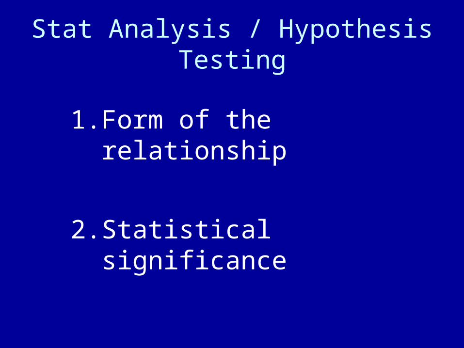
Stat Analysis / Hypothesis Testing

1. Form of the relationship

2. Statistical significance

Variables:Scale by Categorical

• Form of the relationship:

Means of each category (M & F victim)

• Statistical Significance:

Independent samples t-test

Means observed in Sample

Victim Gender Average Sentence

Male 6 months

Female 16 months

Statistical Signficance

• Q: Is this a “statistically significant” difference?

• Can the “null hypothesis” be rejected?

Null hypothesis: there are NO differences in sentencing for male vs. female victims

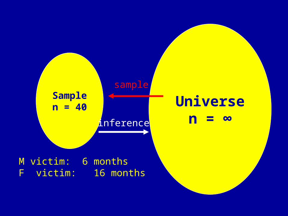
Universen = ∞

Samplen = 40

M victim: 6 monthsF victim: 16 months

sample

inference

Logic of Statistical Inference

• What is the probability of drawing the observed sample (M = 6 months vs. F = 16 months) from a universe with no differences?

• If probability very low, then differences in sample likely reflect differences in universe

• Then null hypothesis can be rejected; difference in sample is statistically significant

Strategy

• Draw an infinite number of samples of n = 40, and graph the distribution of their male victim / female victim differences

Null Hyp:M = 11 monthsF = 11 months

M: 6F: 16

Samples of n = 40 Universe n = ∞

M: 13F: 9

M: 11F: 11

M: 8F: 14

T-test

Sampling distribution: Mean difference

Function of:

1) difference in means

2) variance (dispersion around mean)

Possible Sample -- 1

1 2 3 4 5 6 . . . 16

Male Victim Female Victim


1 2 3 4 5 6 . . . 16

Male Victim Female Victim

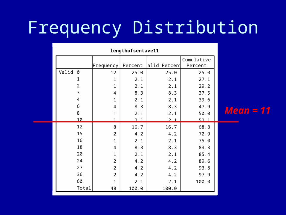
Frequency Distributionlengthofsentave11

12 25.0 25.0 25.0

1 2.1 2.1 27.1

1 2.1 2.1 29.2

4 8.3 8.3 37.5

1 2.1 2.1 39.6

4 8.3 8.3 47.9

1 2.1 2.1 50.0

1 2.1 2.1 52.1

8 16.7 16.7 68.8

2 4.2 4.2 72.9

1 2.1 2.1 75.0

4 8.3 8.3 83.3

1 2.1 2.1 85.4

2 4.2 4.2 89.6

2 4.2 4.2 93.8

2 4.2 4.2 97.9

1 2.1 2.1 100.0

48 100.0 100.0

0

1

2

3

4

6

8

10

12

15

16

18

20

24

27

36

60

Total

ValidFrequency Percent Valid Percent

CumulativePercent

Mean = 11

Variance

x i - Mean )2

Variance = s2 = ----------------------- N

x i - Mean )2

but: s2 = ----------------------- N - 1

Standard Deviation = s = variance

Calculating Variancelengthofsentave11

12 25.0 25.0 25.0

1 2.1 2.1 27.1

1 2.1 2.1 29.2

4 8.3 8.3 37.5

1 2.1 2.1 39.6

4 8.3 8.3 47.9

1 2.1 2.1 50.0

1 2.1 2.1 52.1

8 16.7 16.7 68.8

2 4.2 4.2 72.9

1 2.1 2.1 75.0

4 8.3 8.3 83.3

1 2.1 2.1 85.4

2 4.2 4.2 89.6

2 4.2 4.2 93.8

2 4.2 4.2 97.9

1 2.1 2.1 100.0

48 100.0 100.0

0

1

2

3

4

6

8

10

12

15

16

18

20

24

27

36

60

Total


CumulativePercent

Mean = 11

Variance

Statistics

lengthofsentave1148

0

11.02

12.109

146.617

0

60

Valid

Missing

N

Mean

Std. Deviation

Variance

Minimum

Maximum

t distribution

• Sampling distribution of a difference in means

• Function of mean difference

& “pooled” variance (of both samples)

mean1 – mean2

t = --------------------------------sp√ (1/n1) + (1/n2)


mean dif& var


mean dif& var

mean dif& var

mean dif& var


t


t

t

t

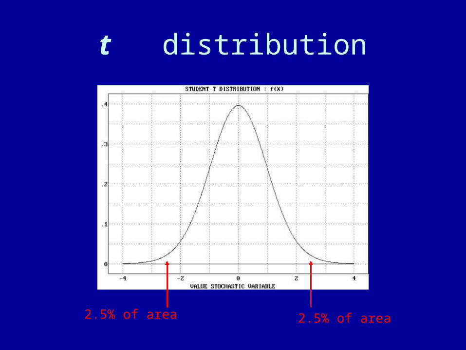
t distribution

2.5% of area2.5% of area

Statistical Significance

• If probability is less than 5 in 100, the null hypothesis can be rejected, and it can be concluded that the difference also exists in the universe.

p < .05

• The finding from the sample is statistically significant

SPSS t-test Output

Group Statistics

24 16.04 12.723 2.597

24 6.00 9.227 1.883

victim genderfemale

male

lengthofsentave11N Mean Std. Deviation

Std. ErrorMean

Independent Samples Test

.824 .369 3.130 46 .003 10.042 3.208 3.584 16.499

3.130 41.951 .003 10.042 3.208 3.567 16.516

Equal variancesassumed

Equal variancesnot assumed

lengthofsentave11F Sig.

Levene's Test forEquality of Variances

t df Sig. (2-tailed)Mean

DifferenceStd. ErrorDifference Lower Upper

95% ConfidenceInterval of the

Difference

t-test for Equality of Means

1. Read means

2. Read Levene’s Test 3. Read p value

Report Findings

• “Assailants were given an average sentence of 16 months when the victims were female, compared to 6 months when the victims were male (df = 46, t = 3.13, p. < .005).”

• “Respondents gave longer sentences when the victims were female (16 months) than when they were male (6 months), a difference that was statistically signficant (df = 46, t = 3.13, p. < .005).”

Statistical Analysesanalysis of variance

( ANOVA )

Psych 250

Winter, 2011

Variable Type Example Commonly-used Statistical Method

Nominal by Nominal blood type by gender

Chi-square

Scale by Nominal GPA by gender

GPA by major

t-test


Scale by Scale weight by heightGPA by SAT

RegressionCorrelation


Dep Var: Length of SentenceIndep var: Major

length of sentence

12 25.0 25.0 25.0

1 2.1 2.1 27.1

4 8.3 8.3 35.4

5 10.4 10.4 45.8

1 2.1 2.1 47.9

1 2.1 2.1 50.0

6 12.5 12.5 62.5

2 4.2 4.2 66.7

6 12.5 12.5 79.2

1 2.1 2.1 81.3

1 2.1 2.1 83.3

2 4.2 4.2 87.5

1 2.1 2.1 89.6

1 2.1 2.1 91.7

1 2.1 2.1 93.8

1 2.1 2.1 95.8

1 2.1 2.1 97.9

1 2.1 2.1 100.0

48 100.0 100.0

0

1

2

3

4

5

6

8

12

15

16

18

24

27

36

42

60

66

Total


CumulativePercent

Mean = 14.6

Variance = 212.4

Statistics

length of sentence48

0

9.98

14.573

212.361

Valid

Missing

N

Mean

Std. Deviation

Variance

Form of Relationship

(differences seen in sample)

Length of Sentence by Major

• Nat sci 14.3

• Soc sci 7.4

• Art & Hum 11.0

Descriptives

lengthofsentave11

19 14.26 15.183 3.483 6.94 21.58 0 60

14 7.43 8.474 2.265 2.54 12.32 0 24

15 10.27 10.067 2.599 4.69 15.84 0 36

48 11.02 12.109 1.748 7.50 14.54 0 60

natural science

social science

arts and humanities

Total

N Mean Std. Deviation Std. Error Lower Bound Upper Bound

95% Confidence Interval forMean

Minimum Maximum

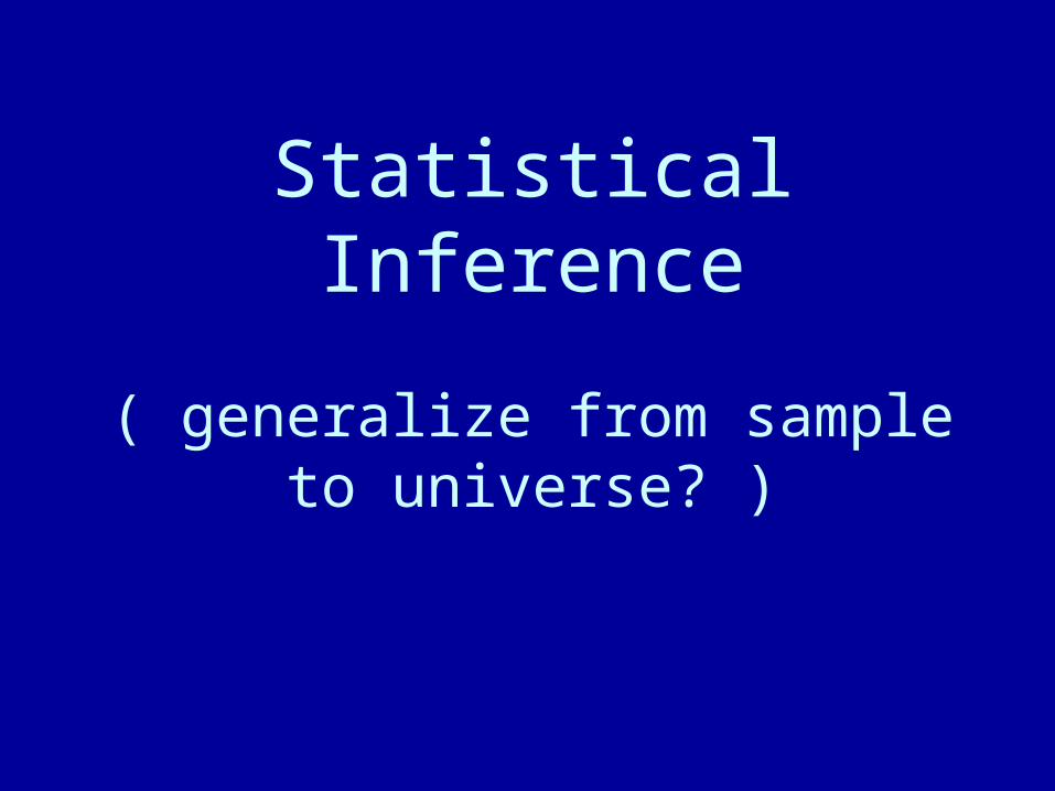
Statistical Inference

( generalize from sample to universe? )

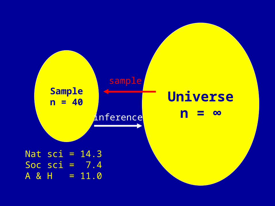
Universen = ∞

Samplen = 40

Nat sci = 14.3Soc sci = 7.4A & H = 11.0

sample

inference


1 2 3 4 5 6 7 8 9 10 11 12 13 14 15

Social Science Art & Human Natural Science

ANOVA Logic

1. Calculate ratio of “between-groups” variance to “within-groups” variance

2. Estimate the sampling distribution of that ratio: F distribution

3. If the probability that the ratio in sample could come from universe with no differences in group means is < .05, can reject null hypothesis and infer that mean differences exist in universe

ANOVA Logic• Between groups:

nsocsci(Meansocsci - Mean)2

+ narthum(Meanarthum - Mean)2

+nnatsci(Meannatsci – Mean)2 / df

• Within groups:

(ni – Meansocsci) 2

+ (ni - Meanarthum)2

+ (ni - Meannatsci) 2 / df

F ratio

between groups mean squares

F =

within groups mean squares

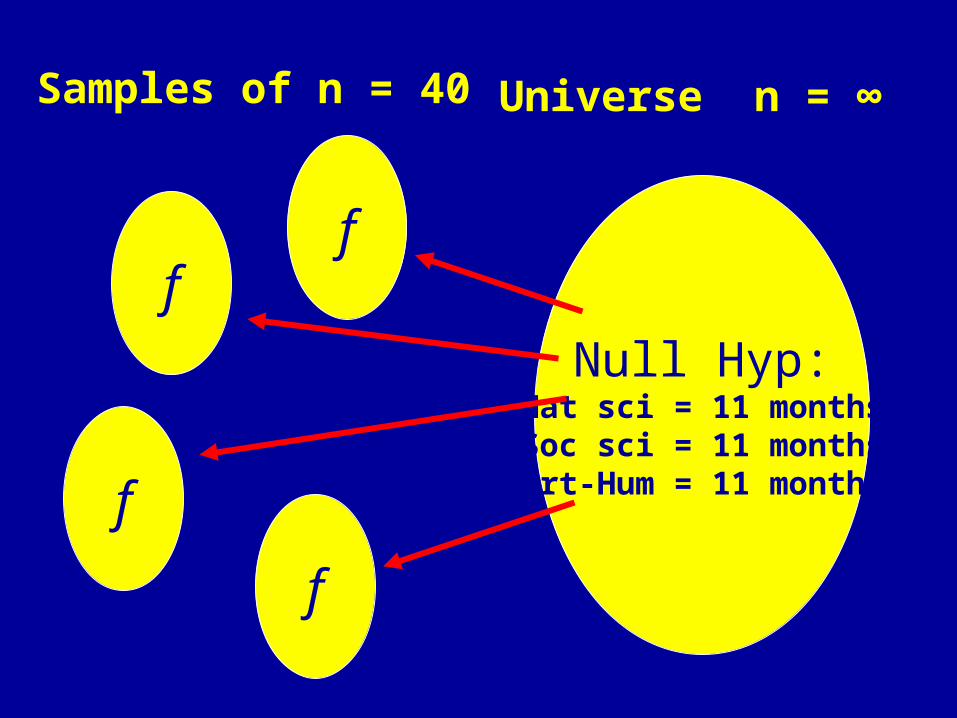
Null Hyp:Nat sci = 11 monthsSoc sci = 11 monthsArt-Hum = 11 months

f


f

f

f

f Distributions

ANOVA: sentence by major

Descriptives

lengthofsentave11

19 14.26 15.183 3.483 6.94 21.58 0 60

14 7.43 8.474 2.265 2.54 12.32 0 24

15 10.27 10.067 2.599 4.69 15.84 0 36

48 11.02 12.109 1.748 7.50 14.54 0 60

natural science

social science

arts and humanities

Total



Minimum Maximum

ANOVA

lengthofsentave11

388.933 2 194.467 1.346 .271

6502.046 45 144.490

6890.979 47

Between Groups

Within Groups

Total

Sum ofSquares df Mean Square F Sig.

ANOVA: sentence by majorsimulated data

Descriptives

lengthofsentave11

19 14.26 15.183 3.483 6.94 21.58 0 60

14 7.43 8.474 2.265 2.54 12.32 0 24

15 10.27 10.067 2.599 4.69 15.84 0 36

48 11.02 12.109 1.748 7.50 14.54 0 60

natural science

social science

arts and humanities

Total



Minimum Maximum

ANOVA

lengthofsentave11

388.933 2 194.467 1.346 .271

6502.046 45 144.490

6890.979 47

Between Groups

Within Groups

Total

Sum ofSquares df Mean Square F Sig.

Write Findings

“Social science majors assigned sentences averaging 7.4 years, arts and humanities students 10.3 years, and natural science students 14.3 years, but these differences were not statistically significant (df = 2, 42, F = 1.35, p < .30).”

statistical analyses t-tests psych 250 winter, 2013

Documents

mean slide

variance slide

gpa slide

significant slide

area slide

months sample inference

statistical significance

months f victim