static stochastic assignment: scilab...
TRANSCRIPT

29/11/2002 1
Static stochastic assignment: Scilab implementation
Elina M. Mancinelli†‡
Collaborative work with P. Lotito† and J.-P. Quadrat†
École d’automne: Modélisation mathématique du trafique automobile
† ‡ CONICET

29/11/2002 2
Plan
• Rθ semirings • Cost measures and decision variables
• Decision variables• Characteristic functions, Fenchel and Cramer transform
• Traffic Assignment• Probrit assignment• Logit assignment
• Dial’s logit• Improved Dial’s logit • Bell’s logit• Markov chain implementation
• Stochastic user equilibrium • Examples

29/11/2002 3
( , , )θθ = ∪ +∞ ⊕ ⊗
( )1 log θ θθ θ
− −+⊕ = − a be ea b
Semiring family
For each θ > 0, we consider the following :
where operations ≈θ and ƒ are given by:
⊗ = +a b a band verify:≈θ:associative, commutative, with zero element ε = +∞.ƒ: associative, with a unit element e = 0 and distributive over
≈θ and zero is absorbing.

29/11/2002 4
For each θ we can consider over a finite set Ω = ωj j=1,n a cost measure
( ) 0jc eθ ω⊕ = =
( ) ( )
1 1
1 log 0 1j jn n
c c
j je eθ ω θ ω
θ− −
= =
= ⇔ =
− ∑ ∑
:c θΩ →Ω is a normalized set if
Through the e-θ . application it is possible to map this in thestandard algebra and to make computations as probabilitiesit can also be seen as linear computations over Rθ .
The limit of this family of semirings as θ→+∞ is the min-plusalgebra, Rmin , composed by (R∪ +∞ , min, +).

29/11/2002 5
Cost measures and decision variables
We call a decision space the triplet (U, U, K) where U is a topological space, U the set of open sets of U and K a mapping from U to Rmin such that
1. K (U)=02. K (∅ )=+∞3. K (∪ n An)=infnK (An ) for any An ∈ U .
The mapping K is called a cost measure.A set of cost measures K is said tight if
sup inf ( )c
KCcompact UC
∈⊂= +∞
KK
A mapping c: U → Rmin such that K (A)=infu ∈ A c(u ) ∀ A⊂ U is called a cost density of the cost measure K.

29/11/2002 6
Theorem (Akian, Kolokoltsov) Given a l.s.c. c with values in Rminsuch that infu c(u ) = 0, the mapping A:U→ K(A)=infu ∈ A c(u )defines a cost measure on (U, U).Conversely any cost measure defined on a topological space with acountable basis of open sets admits a unique minimal extension K*to P(U) (the set of subsets of U) having a density c which is a l.s.c.function on U satisfying infu c(u ) = 0.

29/11/2002 7
Decision variable

29/11/2002 8

29/11/2002 9
29/11/2002 10
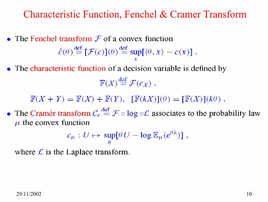
Characteristic Function, Fenchel & Cramer Transform
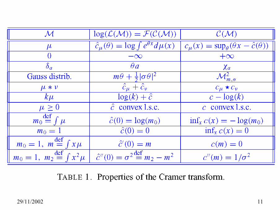
29/11/2002 11

29/11/2002 12
Traffic assignment
Given a transport network G=(N,A) and a transport demand Dthe traffic assignment problem consists in determining the flows fa on the arcs a ∈ A of the network depending on the time spent in each arc ta.In the static stochastic case the perception of the travel time overlinks is random. Let Ta(f): perceived travel time on link a, the perceived travel time on route r ∈ Rpq.
pqrC
Pr( , / )pq pq pqr r l pqP C C l r R c= ≤ ∀ ≠ ∈
( ) ( )
pq pq pqr r r
pq pq pq pqr r r r
C c
E C E c c
ξξ
= +
= + =

29/11/2002 13
Cpq is normally distributed with a mean cpq.. This distribution can be
derived from the distribution of links travel time.
( , ')T MVN t Σ∼Let T=(...,Ta,...), t = (...,ta,...), Σ’=[β.t.I]. Assuming
Let ∆pq be the link-path incidence matrix for O-D pair pq .
(..., , ...) .pq pqr
pqC C T= = ∆
( , ) ,pq pq pqaT MVN c p qΣ ∀∼
Probit-based assignment
Let the joint density functionis given by
'. , .[ . ].pq pq pq pq pqc t t Iβ= ∆ Σ = ∆ ∆
The path-choice probability PX > x, for P a Gaussian law is not explicitly known. Computation of probit assignment is done by Monte Carlo simulation process. [Sheffi85]

29/11/2002 14
Step 0: Initialization. Set l:=1Step 1 : Sampling. Sample
Step 2 : All-or nothing assigment. Based on , assign dpq to theshortest path connecting each O-D pair p-q. We obtain the setof links flows
Step 3 : Flow averaging. LetStep 4 : Stopping test
a) Let
b) If stop. The solution isOtherwise, set l:=l+1 and go to Step 1.
( )2( ) ( ) ( )
1
( 1)l
l m la a
ma X x l l a Aσ
=
= − − ∀ ∈∑
( )( ) ( 1) ( )(1 ) −= − +l l la a ax l x X l
( )( ) ( )max σ κ≤l la a ax ( )l
ax
( ) laT
( ) from ( , )la a a aT T N t tβ∼
Probit-based stochastic network loading algorithm

29/11/2002 15
Another approach to consider the logit assignment is considering that the error in estimating the path travel time has a Gumbel distribution:
θ- x-eeG X > x=
θθ
−−
∈
∈ =∑
trpq tr
r Rpq
er Re
P
Logit-based assignment
In this case la probability to chose a path r to join the OD pair pq is given by
where tr is the measured travel time for path r

29/11/2002 16
θ is the dispersion parameter, it is inversely proportional tothe standard deviation of the perceived path travel time.
If θ is very large the perception error is small and users willtend to select the minimum travel-time path ( logit assignmenttends an all-or-nothing assignment).
In the limit, where θ → 0 the share of flow on all the path willbe equal independently of the path travel-time (a uniform sharingamong all the possible path).

29/11/2002 17
Implemented logit-based assignments
Dial’s logit: [Dial 1971] only efficient path are consider.A path between pq OD pair is efficient iff1... ....ir pp p q=
1 1............ andi i i ip p p qp p p q it t t t+ +< < ∀Denoting Gpq=(N,Apq) the graph obtained eliminating the arcs for which this condition is not satisfied and Opq the node-arc origin incidence matrix (resp. Dpq for destination), we can define the transition weight matrix
Wpq = Opq T (Dpq)’
( ), ataa aaT diag T T e a Aθ−= = ∀ ∈
where

29/11/2002 18
We have, ( )pq
ij aaW T a i j A= ∀ = → ∈
0( )* ( )pq pq i
iW W∞
=∃ = ∑
The logit assignment over efficient path is given by:
∈= ∑ * * *( ) ( ) /( )pq pq pq pq
ij pq pi ij jq pqpq D
F d W W W W
*( )pqpqW : total weight of all efficient path from p to q
* *( ) ( )pq pq pqpi ij jqW W W : total weight of all efficient path using i→j
* * *( ) ( ) /( )pq pq pq pqpi ij jq pqW W W W : probability for a path from p to q of
using i→j for the logit distribution on the efficient paths

29/11/2002 19
Improved Dial’s logit: [Sheffi 1985]: a new definition of efficient path is consider. A path from node p to q is efficient iff
Defining in a similar way a new graph Gp=(N, Ap) and incidencematrices Op , Dp and weight matrix Wp the flow can be computedwith the formula
1... ....ir pp p q=
1...... i ip pp p it t +< ∀
∈= ∑ * *( ) ( )p p p p
ij pi ij jpq D
F W W W D
∈=
* if/e
)0 ls
(e
pp pq pqq
d W pq DD
with

29/11/2002 20
Bell’s logit [Bell 1995]: in this implementation all the paths are used,by remarking that is not necessary to enumerate the paths but to be able to compute star of matrices. But W* = (I-W)-1 is well defined as soon as the spectral radius of W, ρ(W ), smaller than 1.Denoting by W the transition weight matrix for the original graph G
− −
∈= − −∑ 1 1( ) ( ) p
ij pi ij jp N
F I W W I W D
with− − ∈=
1 ifelse
/( )0
p pq pqq
d I W pq DD
The parameter θ must be chosen large enough such that ρ(W ) < 1.
29/11/2002 21
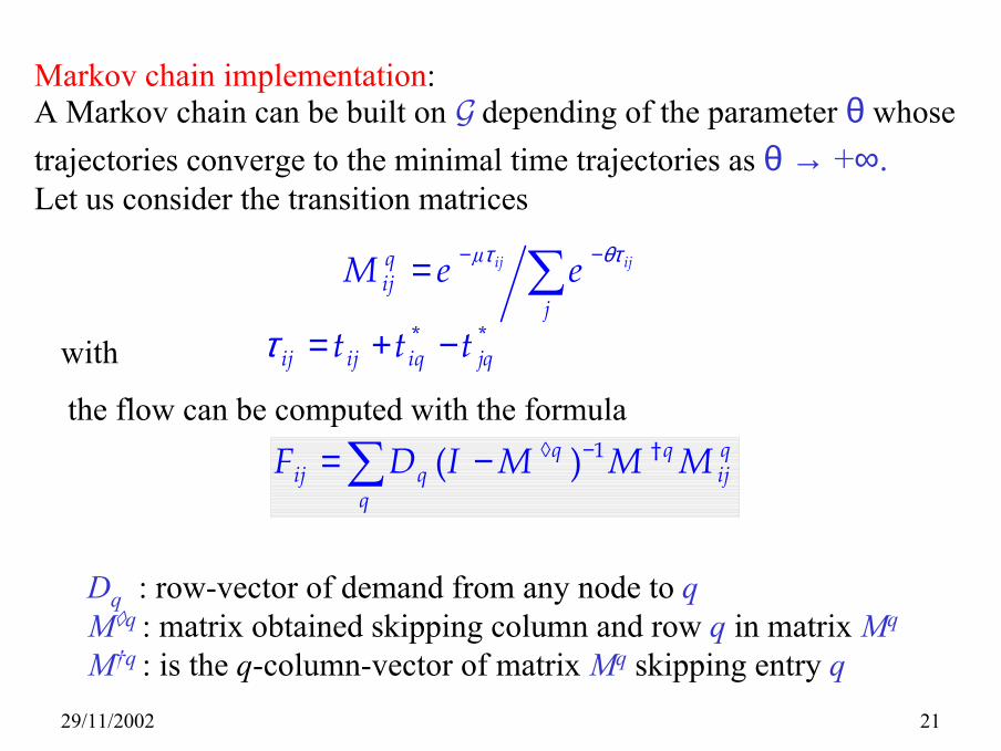
Markov chain implementation:A Markov chain can be built on G depending of the parameter θ whose trajectories converge to the minimal time trajectories as θ → +∞.Let us consider the transition matrices
τ θτ− −= ∑ij ijµqij
jM e e
with τ = + −* *ij ij iq jqt t t
◊ −= −∑ †1( )q q qij q ij
qF D I M M M
Dq : row-vector of demand from any node to qM◊q : matrix obtained skipping column and row q in matrix Mq
M†q : is the q-column-vector of matrix Mq skipping entry q
the flow can be computed with the formula
29/11/2002 22
− −
∈= − −∑F 1 1( ( )) ( ( )) ( ) ( ( )) ( )p
ij p i ij jp N
F I W F W F I W F D F
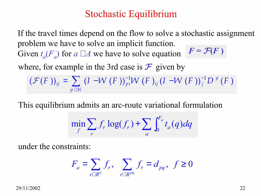
Stochastic Equilibrium
If the travel times depend on the flow to solve a stochastic assignmentproblem we have to solve an implicit function.Given ta(Fa) for a ∈ A we have to solve equation F = F(F )
where, for example in the 3rd case is F given by
This equilibrium admits an arc-route variational formulation
0min log( ) ( )aF
r r af r af f t q dq+∑ ∑∫
, , 0a pq
a r r pqr R r R
F f f d f∈ ∈
= = ≥∑ ∑under the constraints:

29/11/2002 23
The fixed point algorithm
Fn+1 = an Fn +(1- an) F(Fn)
F(Fn) is solution of
min log( ) ( )( )nr r a a a af r a
f f t F F F+ −∑ ∑
which is a partially linearized version of the original minimizationproblem. From the convexity of this last problem we obtain that F(Fn ) - Fn is a descent direction of the original problem.

29/11/2002 24
ExampleLogitB θ =4 LogitB θ = 25
AON

29/11/2002 25
SUE LogitB θ = 10, iter=150 UE DSD Assignment
Difference

29/11/2002 26
AON
LogitD θ =5

29/11/2002 27
Difference
SUE LogitD θ = 60, iter=50UE DSD Assignment

29/11/2002 28
References1. M. Akian “Densities of idempotent measures and large deviations”, AMS 99.2. M. Akian “Theory of cost measures: convergence of decision variables” INRIA, RR-2611, 1995.3. M. Akian “On the continuity of the Cramer Transform”, INRIA, RR-2841, 1996.4. M. Akian, J.P.Quadrat and M. Viot “Duality between probability and optimization”.
Idempotency (Bristol 1994), pp.331-353, Publ. Newton Inst. 11, Cambridge Univ Press, 1998.5. F. Baccelli, G. Cohen, G.J. Olsder, J.P. Quadrat “Synchronization and linearity”, Wiley 1992.6. M.G. Bell “Alternatives to Dial’s Logit assignment algorithm”, Transp. Research, B, vol.29B,
N°4, pp. 287-295, 1995.7. M.G. Bell and Y.Iida “Transportation network analysis”, John Wiley and Sons, 1997.8. E. Cascetta “Transportation systems engineering: theory and methods”, Kluwer-Academic
Publishers, 2001.9. R.B. Dial “A probabilistic multipath traffic assignment model which obviates path enumeration”,
Transp. Research, 5, 1971.10. C.Gomez (Editor): “Engineering and Scientific Computing with Scilab”, Birkhauser 1999 and
(http://www-rocq.inria.fr/scilab/).11. V.N. Kolokoltsov, V.P. Maslov “Idempotent calculus as the apparatus of optimization theory”,
Functional Anal. Appl., Vol. 23, 1989.12. M. Patriksson “The Traffic Assignment Problem, Models and Methods”, VSP Utrech 1994.13. Y. Sheffi “Urban Transportation Networks”, Prentice Hall, 1985.14. S. Erlander, N.F. Stewart “The Gravity Model in Transportation Analysis” VSP Utrech 1990.