static balancing of rigid-body linkages and compliant ...suresh/theses/sangameshphdthesis.pdf ·...
TRANSCRIPT
Static balancing of rigid-body
linkages and compliant mechanisms
A THESIS
SUBMITTED FOR THE DEGREE OF
DOCTOR OF PHILOSOPHY
IN THE FACULTY OF ENGINEERING
by
Sangamesh Deepak R
Department of Mechanical Engineering
Indian Institute of Science
Bangalore – 560012, INDIA
MAY 2012

c© Copyright by Sangamesh Deepak R 2013
All Rights Reserved
ii
Abstract
Static balance is the reduction or elimination of the actuating effort in quasi-static
motion of a mechanical system by adding non-dissipative force interactions to the
system. In recent years, there is increasing recognition that static balancing of elastic
forces in compliant mechanisms leads to increased efficiency as well as good force
feedback characteristics. The development of insightful and pragmatic design meth-
ods for statically balanced compliant mechanisms is the motivation for this work.
In our approach, we focus on a class of compliant mechanisms that can be approxi-
mated as spring-loaded rigid-link mechanisms. Instead of developing static balancing
techniques directly for the compliant mechanisms, we seek analytical balancing tech-
niques for the simplified spring–loaded rigid–link approximations. Towards that, we
first provide new static balancing techniques for a spring-loaded four-bar linkage. We
also find relations between static balancing parameters of the cognates of a four-bar
linkage. Later, we develop a new perfect static balancing method for a general n-
degree-of-freedom revolute and spherical jointed rigid-body linkages. This general
method distinguishes itself from the known techniques in the following respects:
1. It adds only springs and not any auxiliary bodies.
2. It is applicable to linkages having any number of links connected in any manner.
3. It is applicable to both constant (i.e., gravity type) and linear spring loads.
4. It works both in planar and spatial cases.
This analytical method is applied on the approximated compliant mechanisms as
well. Expectedly, the compliant mechanisms would only be approximately balanced.
iii
We study the effectiveness of this approximate balance through simulations and a
prototype. The analytical static balancing technique for rigid-body linkages and the
study of its application to approximated compliant mechanisms are among the main
contributions of this thesis.
iv
Acknowledgements
The motivating idea for this work is that static balancing techniques for compliant
mechanisms can be developed by extracting insights from static balancing techniques
for rigid-body linkages. The originality of this idea belongs to my advisor, Prof. G.
K. Ananthasuresh. Further, I had regular meetings with my advisor where he offered
his comments and suggestions on my work. Some of his suggestions helped me in
directing this work to this form. I also appreciate his emphasis on prototypes and
the support system he has developed for making them. He has spent significant time
in sharing his experiences and opinions on technical writing. These were valuable in
documenting my work.
In making prototypes presented in the thesis, I had received help from Mr. A.
Ravikumar, Mr. Ramu G., Mr. B. M. Vinod Kumar and Mr. Praveenraj H. K. I
deeply value their knowledge and skills. I also acknowledge the co-operation that I
received from Mr. A. Raja in accessing the workshop.
Almost all the fabrication aspects of the prototype presented in Appendix G was
handled by Mr. Amrith Hansoge. I deeply value his industrial experience, which were
crucial in making a rather impressive prototype.
Prof. Ashitava Ghosal, advisor for my master’s thesis, was very helpful during my
transition from master’s to PhD. I also appreciate the remarkable care he took to see
that I choose a topic of research that suits me.
My course-work in IISc has been one of the most exciting and satisfying aspects
of my life in IISc. I immensely thank all the instructors for their effort in getting
us exposed to challenging concepts. Prof. C. R. Pradeep’s class on Topology ranks
as the best class that I ever had in my academic career. Courses such as these have
v

helped me a lot.
Another exciting aspect of my stay in IISc was the weekly group meeting that Prof.
Ananthasuresh conducts. Through these meetings, my advisor and my colleagues in
the lab gave me an exposure to diverse areas of knowledge and research. In an
association spanning a little less than five years, I probably have many things to say
about my advisor. However, I will sum up this association like this – it has been
mostly a pleasure and definitely a privilege.
My lab-mates have been invariably nice, co-operative and understanding. I feel
very privileged to be part of such a good set of people.
A lot of people formed the source for many exciting academic exchanges that I
had. Among them, I would like to make a special mention of Narayana Reddy, Kali-
das, Meenakshi Sundaram, Hariharan and Sreenath. These exchanges have helped
me to put my attention on some of the fundamental principles in mechanics and
mathematics in general.
While my interaction with people in IISc is somewhat less, I must nevertheless
acknowledge that in general people have been kind and understanding towards me. I
would like to specially thank many mess workers who served me with food even if I
was late many times.
The physical training that I received from Master Stephen Kumar, Master Man-
junath and my senior Rahul S., has been one of the best things to happen in my life.
This training helped me to maintain my mental balance even in depressing times.
On personal front, my mother absorbed all the shocks, pulls and pressure to
ensure a free ambience for my growth. It was because of this free ambience that
my understanding of science and mathematics matured over the years. Patience,
perseverance, hope, courage, endurance and wisdom displayed by my mother are
inspirational. I also acknowledge the care shown by my father towards my well-being.
vi
Contents
Abstract iii
Acknowledgements v
1 Introduction 1
1.1 What is static balance? . . . . . . . . . . . . . . . . . . . . . . . . . . 1
1.1.1 Static balance of rigid-body linkages . . . . . . . . . . . . . . 2
1.1.2 Compliant mechanisms and its static balance . . . . . . . . . . 9
1.1.3 Static balance: rigid-body linkage vs. compliant mechanisms . 11
1.2 Motivation for the thesis . . . . . . . . . . . . . . . . . . . . . . . . . 11
1.3 Scope of the thesis . . . . . . . . . . . . . . . . . . . . . . . . . . . . 14
1.3.1 Three methods to statically balance a zero-free-length spring-
loaded four-bar linkage . . . . . . . . . . . . . . . . . . . . . . 14
1.3.2 Static balancing of cognates . . . . . . . . . . . . . . . . . . . 14
1.3.3 Static balancing of revolute-jointed linkages without auxiliary
links . . . . . . . . . . . . . . . . . . . . . . . . . . . . . . . . 15
1.3.4 Static balancing of spatial and/or revolute jointed linkages
without auxiliary links . . . . . . . . . . . . . . . . . . . . . . 15
1.3.5 Static balancing of flexure-based compliant mechanisms by ad-
dition of springs . . . . . . . . . . . . . . . . . . . . . . . . . . 15
2 Literature Survey 17
2.1 Rigid-body linkages under gravity loads . . . . . . . . . . . . . . . . . 17
2.1.1 Counter-weight balancing . . . . . . . . . . . . . . . . . . . . 17
vii

2.1.2 Balancing by addition of springs . . . . . . . . . . . . . . . . . 18
2.2 Rigid linkages under spring loads . . . . . . . . . . . . . . . . . . . . 21
2.3 Static balance of compliant mechanisms . . . . . . . . . . . . . . . . . 22
2.4 Prior Art . . . . . . . . . . . . . . . . . . . . . . . . . . . . . . . . . 23
2.4.1 Preliminaries . . . . . . . . . . . . . . . . . . . . . . . . . . . 24
2.4.2 Plagiograph . . . . . . . . . . . . . . . . . . . . . . . . . . . . 27
2.4.3 Derivation of the balancing solution in [1] . . . . . . . . . . . 28
3 Static balancing of a four-bar 36
3.1 Introduction . . . . . . . . . . . . . . . . . . . . . . . . . . . . . . . . 36
3.2 Static balancing of a given spring-loaded four-bar linkage . . . . . . . 37
3.2.1 Technique 1 . . . . . . . . . . . . . . . . . . . . . . . . . . . . 38
3.2.2 Technique 2 . . . . . . . . . . . . . . . . . . . . . . . . . . . . 40
3.2.3 Technique 3 . . . . . . . . . . . . . . . . . . . . . . . . . . . . 43
3.3 A prototype with technique 2 . . . . . . . . . . . . . . . . . . . . . . 48
4 Static balance of the cognates 51
4.1 Introduction . . . . . . . . . . . . . . . . . . . . . . . . . . . . . . . . 51
4.1.1 Cognates . . . . . . . . . . . . . . . . . . . . . . . . . . . . . . 51
4.1.2 Static balancing parameters and the cognates . . . . . . . . . 52
4.2 A geometric problem and its solution . . . . . . . . . . . . . . . . . . 54
4.2.1 Case (i): a, b and c are parallel. . . . . . . . . . . . . . . . . . 58
4.2.2 Case (ii): a, b and c are concurrent. . . . . . . . . . . . . . . . 59
4.2.3 Case (iii): a, b, and c are neither parallel nor concurrent. . . . 59
4.2.4 Finding the focal pivot . . . . . . . . . . . . . . . . . . . . . . 61
4.3 The result . . . . . . . . . . . . . . . . . . . . . . . . . . . . . . . . . 63
4.3.1 A parameterization of the balancing parameters of the three
cognates that has cognate triangle related invariants . . . . . . 63
5 Static balancing of planar linkages 66
5.1 Introduction . . . . . . . . . . . . . . . . . . . . . . . . . . . . . . . . 66
5.2 Balancing a lever . . . . . . . . . . . . . . . . . . . . . . . . . . . . . 67
viii
5.2.1 Potential energy as a function of the configuration variable . . 68
5.2.2 Invariance of potential energy with respect to the configuration
variable . . . . . . . . . . . . . . . . . . . . . . . . . . . . . . 71
5.3 Balancing of a rigid body in a plane . . . . . . . . . . . . . . . . . . . 74
5.4 New static balancing techniques for revolute-jointed linkages . . . . . 80
5.4.1 The potential energy of loads on a body transformed as a func-
tion of another body . . . . . . . . . . . . . . . . . . . . . . . 80
5.4.2 Proposition 2 as the recursive relation of an iterative static
balancing algorithm . . . . . . . . . . . . . . . . . . . . . . . . 82
5.4.3 Static balancing of any revolute-jointed linkages with any kind
of zero-free-length spring and constant load interaction within
the linkage . . . . . . . . . . . . . . . . . . . . . . . . . . . . . 96
5.5 A note on prismatic joint . . . . . . . . . . . . . . . . . . . . . . . . . 99
6 Static balancing of spatial linkages 102
6.1 Introduction . . . . . . . . . . . . . . . . . . . . . . . . . . . . . . . . 102
6.2 The class of functions in feature 1 . . . . . . . . . . . . . . . . . . . . 103
6.3 Joints that can potentially satisfy feature 2 . . . . . . . . . . . . . . . 104
6.4 Spherical joint has feature 2 . . . . . . . . . . . . . . . . . . . . . . . 107
6.5 Revolute joint has feature 2 . . . . . . . . . . . . . . . . . . . . . . . 109
6.6 Algorithm to synthesize static balancing solution of a spatial revolute/spherical-
jointed tree-structured linkage having zero-free-length spring and/or
gravity loads exerted by a reference link . . . . . . . . . . . . . . . . 111
6.6.1 Illustrative example . . . . . . . . . . . . . . . . . . . . . . . . 113
6.7 Static balance of any kind of spatial revolute and/or spherical jointed
linkage with constant load and zero-free-length spring load interaction 116
6.8 A note . . . . . . . . . . . . . . . . . . . . . . . . . . . . . . . . . . . 116
7 Static balance of compliant mechanisms 118
7.1 Balancing a flexure beam . . . . . . . . . . . . . . . . . . . . . . . . . 119
7.1.1 The flexure beam . . . . . . . . . . . . . . . . . . . . . . . . . 119
7.1.2 Rigid-body model for the flexure beam . . . . . . . . . . . . . 120
ix

7.1.3 Approximation of torsional spring by zero-free-length spring . 122
7.1.4 Static balancing by addition of a zero-free-length spring . . . . 126
7.1.5 Balancing springs on the flexure beam . . . . . . . . . . . . . 130
7.2 Framework . . . . . . . . . . . . . . . . . . . . . . . . . . . . . . . . . 133
7.3 Flexure-based compliant four-bar mechanism . . . . . . . . . . . . . . 136
7.3.1 Description of the mechanism . . . . . . . . . . . . . . . . . . 136
7.3.2 Step 1 . . . . . . . . . . . . . . . . . . . . . . . . . . . . . . . 138
7.3.3 Step 2 – The effort function . . . . . . . . . . . . . . . . . . . 138
7.3.4 Step 3 . . . . . . . . . . . . . . . . . . . . . . . . . . . . . . . 139
7.3.5 Step 4 – Static balance of the linkage under zero-free-length
spring load . . . . . . . . . . . . . . . . . . . . . . . . . . . . 140
7.3.6 Step 5 – Approximate static balance of flexure-based four-bar
linkage . . . . . . . . . . . . . . . . . . . . . . . . . . . . . . . 142
7.3.7 A way to improve the static balance of the flexure-based four-
bar linkage . . . . . . . . . . . . . . . . . . . . . . . . . . . . . 142
7.4 Another flexure-based four-bar linkage . . . . . . . . . . . . . . . . . 145
7.4.1 Description of the mechanism . . . . . . . . . . . . . . . . . . 145
7.4.2 Step 1 . . . . . . . . . . . . . . . . . . . . . . . . . . . . . . . 147
7.4.3 Step 2 . . . . . . . . . . . . . . . . . . . . . . . . . . . . . . . 147
7.4.4 Step 3 . . . . . . . . . . . . . . . . . . . . . . . . . . . . . . . 147
7.4.5 Step 4 . . . . . . . . . . . . . . . . . . . . . . . . . . . . . . . 149
7.4.6 Step 5 . . . . . . . . . . . . . . . . . . . . . . . . . . . . . . . 149
7.4.7 First order correction . . . . . . . . . . . . . . . . . . . . . . . 149
7.4.8 Prototype . . . . . . . . . . . . . . . . . . . . . . . . . . . . . 150
7.5 Flexure-based 2R compliant mechanism . . . . . . . . . . . . . . . . . 152
7.5.1 Description of the compliant mechanism . . . . . . . . . . . . 152
7.5.2 Step 1: . . . . . . . . . . . . . . . . . . . . . . . . . . . . . . . 152
7.5.3 Step 2 – Identification of effort function . . . . . . . . . . . . . 153
7.5.4 Step 3 . . . . . . . . . . . . . . . . . . . . . . . . . . . . . . . 153
7.5.5 Step 4 . . . . . . . . . . . . . . . . . . . . . . . . . . . . . . . 153
7.5.6 Step 5 . . . . . . . . . . . . . . . . . . . . . . . . . . . . . . . 157
x

7.6 Discussion . . . . . . . . . . . . . . . . . . . . . . . . . . . . . . . . . 157
7.6.1 Static balancing of compliant mechanisms by individually bal-
ancing flexures . . . . . . . . . . . . . . . . . . . . . . . . . . 159
7.6.2 Static balancing of compliant mechanisms using rigid-body link-
ages . . . . . . . . . . . . . . . . . . . . . . . . . . . . . . . . 161
8 Conclusion 163
8.1 A summary of new static balancing techniques for spring and/or
gravity-loaded rigid-body linkages . . . . . . . . . . . . . . . . . . . . 164
8.1.1 Static balancing of a four-bar linkage loaded by a spring on its
coupler link . . . . . . . . . . . . . . . . . . . . . . . . . . . . 164
8.1.2 Static balancing parameters and the cognates of a four-bar linkage164
8.1.3 Static balancing without auxiliary bodies–planar case . . . . . 165
8.1.4 Static balancing without auxiliary bodies–spatial case . . . . . 165
8.2 A framework for designing statically balanced compliant mechanisms 165
8.3 The novelty of the contribution in the context of the current literature 166
8.4 Future work . . . . . . . . . . . . . . . . . . . . . . . . . . . . . . . . 168
A Proofs on finding the focal pivot 169
A.1 If Ia,b and Ic,a circles are coincident, then the given lines a, b and c has
to be concurrent . . . . . . . . . . . . . . . . . . . . . . . . . . . . . . 169
A.2 When M and A are distinct, M is the focal pivot. (Refer to section
(4.2.4 and figure (4.11).) . . . . . . . . . . . . . . . . . . . . . . . . . 170
B An elementary theorem 172
C Normal springs 173
D Satisfying Constraints 175
D.1 Satisfying constraints (5.12), (5.13) and (5.14) . . . . . . . . . . . . . 175
D.2 Satisfying constraints (5.19), (5.20) and (5.21) . . . . . . . . . . . . . 177
E Solving balancing constraints – spatial case 178
xi
F Virtual work calculations 181
F.1 Calculation of stiffness in case 3a based on case 2a . . . . . . . . . . . 186
F.1.1 Obtaining Fx vs. ux in case 2a using virtual work balance . . 186
F.1.2 Obtaining Fx vs. ux in case 3a using virtual work balance . . 191
F.2 Verification of static balance in case 3b through virtual work balance 195
F.3 A first order correction to balancing springs on the flexure-based four-
bar linkage . . . . . . . . . . . . . . . . . . . . . . . . . . . . . . . . . 198
G Another compliant mechanism balancing 207
H Springs between successive links 212
Bibliography 216
xii
List of Tables
3.1 Summary of different techniques to statically balance a spring-loaded
four-bar linkage presented in this chapter . . . . . . . . . . . . . . . . 47
4.1 Deduction of various quantities in equations (3.1 – 3.7) from the cog-
nate triangle . . . . . . . . . . . . . . . . . . . . . . . . . . . . . . . 54
4.2 Ratio of spring constants of balancing spring 1 for three cognates . . 64
5.1 Potential energy of the weight and the zero-free-length component of
the spring acting on the lever is a linear combination of cos θ, sin θ,
and 1. . . . . . . . . . . . . . . . . . . . . . . . . . . . . . . . . . . . 71
5.2 Potential energy of weight and spring acting on a link moving in a plane. 75
5.3 Details of the loads in figure (5.5). It may be checked that the loads
satisfy equations (5.12 – 5.14 ) . . . . . . . . . . . . . . . . . . . . . 77
6.1 The potential in the general form shown in figure (6.3), can be ex-
pressed as a linear combination of the basis functions shown in the
table. Each basis function in the table is a function of translational
variable r and the Z-X-Z Euler angle α, β and γ . . . . . . . . . . . . 105
7.1 Relevant quantities to calculate the torsional stiffness of the spring . . 120
7.2 Virtual work calculation for lever in case (2a) . . . . . . . . . . . . . 124
7.3 Virtual work calculation and slope of Fx vs. ux . . . . . . . . . . . . 125
7.4 Verification of equations (5.10–5.11) being satisfied . . . . . . . . . . 129
7.5 Verification of static balance through virtual work calculations . . . . 129
xiii

7.6 The origin and the slope of Fx vs. ux being matched between case 2a
and case 3a . . . . . . . . . . . . . . . . . . . . . . . . . . . . . . . . 140
7.7 Verification of equations (5.19 - 5.21) for the spring-loaded 2R linkage
of figure (7.14) . . . . . . . . . . . . . . . . . . . . . . . . . . . . . . 140
7.8 Details of the flexure and calculation of torsional spring constant . . . 147
7.9 Matching value and slopes at the origin of the effort function . . . . . 148
7.10 Details of the original spring and balancing spring . . . . . . . . . . . 149
7.11 First order correction of balancing spring parameters . . . . . . . . . 150
7.12 Details of flexure and calculation of torsional spring constant. . . . . 153
7.13 The value and the first derivative of F vs. u at u = 0 . . . . . . . . 154
7.14 Verification of static balance of springs in case 3b . . . . . . . . . . . 157
xiv

List of Figures
1.1 A lever having two discrete equilibrium configurations, namely (b) and
(c) while (a) is not in equilibrium. . . . . . . . . . . . . . . . . . . . . 3
1.2 A lever having a continuous set of equilibrium configurations; it is in
static balance. . . . . . . . . . . . . . . . . . . . . . . . . . . . . . . . 3
1.3 A statically balanced lever as a manually operated road barrier. (Source:
http://www.panoramio.com/photo/42452078) . . . . . . . . . . . . . 4
1.4 Counterweight balancing in a two degree-of-freedom linkage . . . . . 5
1.5 Spring-based balancing in a two degree-of-freedom linkage . . . . . . 5
1.6 Spring-based balancing of a lever . . . . . . . . . . . . . . . . . . . . 6
1.7 Effects of free-length and pre-tension on force-distance plot of a linear
extension spring . . . . . . . . . . . . . . . . . . . . . . . . . . . . . . 8
1.8 A compliant crimper . . . . . . . . . . . . . . . . . . . . . . . . . . . 10
1.9 A spring-loaded four-bar linkage to be statically balanced . . . . . . . 12
1.10 A static balancing solution for the spring-loaded four-bar linkage by
addition of auxiliary links and springs . . . . . . . . . . . . . . . . . . 13
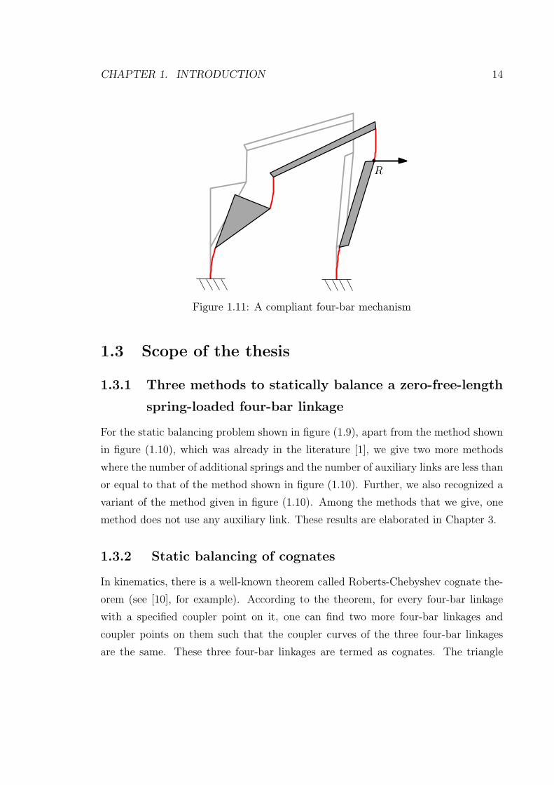
1.11 A compliant four-bar mechanism . . . . . . . . . . . . . . . . . . . . 14
2.1 A counter balancing technique for serial revolute jointed linkages . . . 18
2.2 Use of auxiliary links (colored in grey) along with springs in an existing
technique for balancing a n-degree-of-freedom linkage under constant
load. . . . . . . . . . . . . . . . . . . . . . . . . . . . . . . . . . . . . 19
2.3 A basic spring force balancer . . . . . . . . . . . . . . . . . . . . . . . 24
2.4 A lever with ordinary springs . . . . . . . . . . . . . . . . . . . . . . 25
2.5 Balanced parallelogram . . . . . . . . . . . . . . . . . . . . . . . . . . 25
xv
2.6 Balanced two degree-of-freedom parallelogram linkage . . . . . . . . . 26
2.7 Composition of two zero-length-spring into an equivalent one. The virtual,
equivalent spring between E and D is shown in grey color. . . . . . . . . 27
2.8 A plagiograph or a skew pantograph linkage . . . . . . . . . . . . . . . . 28
2.9 A balanced parallelogram with one its spring along a diagonal decom-
posed into two springs. . . . . . . . . . . . . . . . . . . . . . . . . . . 29
2.10 The parallelogram linkage with a duplicate that maintains a constant
angle of α from the original . . . . . . . . . . . . . . . . . . . . . . . 30
2.11 Synchronization of motion between two parallelogram linkages . . . . 31
2.12 Scaling the duplicate parallelogram linkage . . . . . . . . . . . . . . . 32
2.13 Removal of a spring and compensating it with increase in stiffness of
another spring . . . . . . . . . . . . . . . . . . . . . . . . . . . . . . . 33
2.14 Removal of two more links. . . . . . . . . . . . . . . . . . . . . . . . . 33
2.15 The current literature and our contributions . . . . . . . . . . . . . . 35
3.1 A four-bar linkage with a zero-free-length spring anchored from its
coupler to the ground . . . . . . . . . . . . . . . . . . . . . . . . . . . 37
3.2 Possibility of the four-bar linkage being statically balanced as it is . . 38
3.3 A balanced parallelogram on the load spring . . . . . . . . . . . . . . 39
3.4 Technique 1: Static balancing with two auxiliary links and one balanc-
ing spring . . . . . . . . . . . . . . . . . . . . . . . . . . . . . . . . . 39
3.5 Forming a parallelogram using two auxiliary links. . . . . . . . . . . 40
3.6 A virtual spring between opposite vertices of the parallelogram AFED. 41
3.7 Adding balancing spring 2 across opposite vertices of the parallelogram
to balance the load spring and balancing spring 1. . . . . . . . . . . . 41
3.8 Option 2 for balancing the four-bar linkage without requiring auxiliary
links . . . . . . . . . . . . . . . . . . . . . . . . . . . . . . . . . . . . 42
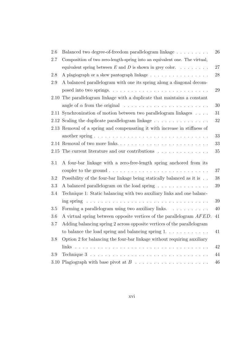
3.9 Technique 3 . . . . . . . . . . . . . . . . . . . . . . . . . . . . . . . . 44
3.10 Plagiograph with base pivot at B . . . . . . . . . . . . . . . . . . . . 46
xvi

3.11 A prototype of four-bar linkage that is statically balanced using option
2. The four-bar linkage seen in the above figure is a Watt’s straight-line
mechanism. . . . . . . . . . . . . . . . . . . . . . . . . . . . . . . . . 48
3.12 Realization of a zero-free length spring . . . . . . . . . . . . . . . . . 49
4.1 The cognates of a four-bar mechanism taking a load spring along their
common coupler curve . . . . . . . . . . . . . . . . . . . . . . . . . . 52
4.2 A cognate triangle and the ground anchor point of a load spring . . . 55
4.3 Technique 3: the base pivot of the plagiograph (U) and the base of the
balanced parallelogram (W) for every cognate are not coincident. . . 55
4.4 Technique 3: the base pivot of the plagiograph (U) and the base of the
balanced parallelogram (W) for every cognate are coincident. . . . . . 56
4.5 Technique 2: the base of the balanced parallelogram (W) at the indi-
cated vertices of the cognate triangle. . . . . . . . . . . . . . . . . . . 57
4.6 A problem in planar geometry . . . . . . . . . . . . . . . . . . . . . . 58
4.7 Finding Sa, Sb, and Sc in case (i) . . . . . . . . . . . . . . . . . . . . 58
4.8 Finding Sa, Sb, and Sc in case (ii) . . . . . . . . . . . . . . . . . . . . 59
4.9 Description of focal pivot . . . . . . . . . . . . . . . . . . . . . . . . . 60
4.10 Points A2, B2 and C2 form a solution to Sa, Sb and Sc . . . . . . . . 60
4.11 Geometric construction to find the focal pivot . . . . . . . . . . . . . 62
5.1 Lack of methods for spring-based n-body linkage balancing without the
usage of auxiliary bodies . . . . . . . . . . . . . . . . . . . . . . . . . 68
5.2 A lever under a constant load and a spring load . . . . . . . . . . . . 69
5.3 Static balancing of a weight by a spring . . . . . . . . . . . . . . . . . 72
5.4 A body that is free to move in a plane . . . . . . . . . . . . . . . . . 74
5.5 A rigid body moving freely in a plane under a constant load is made to
have θ-independent potential energy by addition of two zero-free-length
springs . . . . . . . . . . . . . . . . . . . . . . . . . . . . . . . . . . . 77
5.6 The gravity-loaded serial 4R linkage to be statically balanced. . . . . 86
5.7 Details of Iteration 1 . . . . . . . . . . . . . . . . . . . . . . . . . . . 87
5.8 Details of Iteration 2 . . . . . . . . . . . . . . . . . . . . . . . . . . . 88
xvii
5.9 Details of Iteration 3 . . . . . . . . . . . . . . . . . . . . . . . . . . . 89
5.10 Details of Iteration 4 . . . . . . . . . . . . . . . . . . . . . . . . . . . 90
5.11 Statically balanced gravity-loaded serial 4R linkage. . . . . . . . . . . 91
5.12 Statically balanced serial 3R linkage . . . . . . . . . . . . . . . . . . . 93
5.13 Statically balanced serial 2R linkage . . . . . . . . . . . . . . . . . . . 94
5.14 Details of static balance of a 2R linkage under spring load . . . . . . 95
5.15 Details of static balance of a 4R tree-structure linkage under a constant
load and a spring load . . . . . . . . . . . . . . . . . . . . . . . . . . 96
5.16 Potential Energy variation of spring loads, constant loads, and their sum 97
5.17 Breaking a problem as a superposition of several problem with each
problem being static balance of revolute-jointed tree-structured linkage
with loads exerted by the root body . . . . . . . . . . . . . . . . . . 98
5.18 Static balance of a tree-structured linkage with inter-body load inter-
actions . . . . . . . . . . . . . . . . . . . . . . . . . . . . . . . . . . . 100
5.19 Balancing the lever lever loads in the second load set of figure (5.18) . 101
6.1 Details of static balancing of six degree-of-freedom spatial balancing
under gravity loads . . . . . . . . . . . . . . . . . . . . . . . . . . . . 114
7.1 Details of the flexure beam . . . . . . . . . . . . . . . . . . . . . . . . 119
7.2 Our attention is on reducing horizontal force for a range of horizontal
displacements of point P . . . . . . . . . . . . . . . . . . . . . . . . . 121
7.3 Small-length-flexure model applied to the flexure beam . . . . . . . . 122
7.4 Approximation of the torsional spring by a zero-free-length spring . . 123
7.5 The approximate match in Fx vs. ux relation between case 2a and case
3a . . . . . . . . . . . . . . . . . . . . . . . . . . . . . . . . . . . . . 127
7.6 Static balance of the approximated zero-free-length spring-loaded lever
by addition of a zero-free-length spring . . . . . . . . . . . . . . . . . 128
7.7 All the cases related to the flexure and its approximation by the spring-
loaded lever . . . . . . . . . . . . . . . . . . . . . . . . . . . . . . . . 131
7.8 Fx vs. ux relation obtained from finite element analysis of the flexure
beam . . . . . . . . . . . . . . . . . . . . . . . . . . . . . . . . . . . . 132
xviii

7.9 A consolidated plot of Fx vs. ux for flexure beam and its rigid-body
models . . . . . . . . . . . . . . . . . . . . . . . . . . . . . . . . . . . 134
7.10 A flexure-based four-bar linkage. . . . . . . . . . . . . . . . . . . . . . 137
7.11 The quadrilateral formed by the centers of the flexures . . . . . . . . 137
7.12 Approximation of the flexure-based four-bar linkage as a rigid-body
four-bar linkage with torsional springs. . . . . . . . . . . . . . . . . . 138
7.13 Approximation of torsional springs by zero-free-length springs . . . . 139
7.14 Static balancing by addition of zero-free-length springs . . . . . . . . 141
7.15 A consolidated figure of all the cases . . . . . . . . . . . . . . . . . . 142
7.16 Finite element simulation results for case 1a and case 1b . . . . . . . 143
7.17 Fx vs. ux after first order correction to the stiffness of balancing springs144
7.18 FX vs. ux plot for all the cases shown in figure (7.15) . . . . . . . . . 145
7.19 Consolidated figure containing all the cases . . . . . . . . . . . . . . . 146
7.20 Effort function in all the cases . . . . . . . . . . . . . . . . . . . . . . 148
7.21 A prototype to demonstrate reduction in effort . . . . . . . . . . . . . 151
7.22 A consolidation of all the cases . . . . . . . . . . . . . . . . . . . . . 152
7.23 Details of springs . . . . . . . . . . . . . . . . . . . . . . . . . . . . . 154
7.24 Fx vs. u in two views . . . . . . . . . . . . . . . . . . . . . . . . . . . 155
7.25 Fy vs. u in two views . . . . . . . . . . . . . . . . . . . . . . . . . . . 156
7.26 Plot of effort function when flexure length is increased three-fold . . . 159
7.27 Ideal circular arc-like and non-ideal deformation of flexures . . . . . . 160
7.28 Static balancing of each of the flexures, independently of one another 161
8.1 The current literature and our contributions . . . . . . . . . . . . . . 167
A.1 Ia,b and Ic,a circles are coincident . . . . . . . . . . . . . . . . . . . . 170
A.2 Ia,b is at M . . . . . . . . . . . . . . . . . . . . . . . . . . . . . . . . 171
F.1 l, the length of a diagonal of the quadrilateral of four-bar bar linkage
is used as a convenient configuration defining parameter. . . . . . . . 181
G.1 A compliant gripper compensated by a small spring loaded 2R linkage.
(Basement board dimension: 2.5 feet × 2.5 feet) . . . . . . . . . . . 208
xix

G.2 A statically balanced parallelogram and its modification . . . . . . . 209
G.3 A compliant gripper . . . . . . . . . . . . . . . . . . . . . . . . . . . 210
H.1 A tree-structured linkage under gravity load . . . . . . . . . . . . . . 213
xx
Chapter 1
Introduction
Overview
• The concept of static balance.
• The importance of statically balancing a rigid-body linkage.
• Zero-free-length springs, their importance and their practical realization.
• The importance of statically balancing a compliant mechanism.
• The motivation of the thesis.
• The contributions of the thesis.
1.1 What is static balance?
A system is said to be in static balance if it can undergo quasi-static motion without
any external effort when any dissipative force interactions in the system are removed.
In the general motion of a system, at any configuration, inertia forces of the system,
conservative and dissipative force interactions within the system and external forces
acting on the system are in equilibrium. However, in the motion of a statically
1

CHAPTER 1. INTRODUCTION 2
balanced system, the conservative force interactions have to be in equilibrium by
themselves.
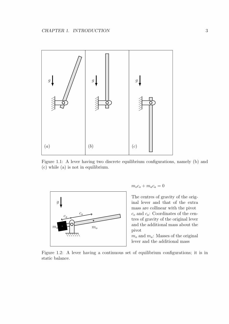
Consider the lever shown in figure (1.1a). The conservative force interactions on
it are the gravity between the lever and the ground and the constraint force between
the lever and the pivot-post (fixed to the ground). If, at a configuration, these forces
could be in equilibrium by themselves then we call the configuration as equilibrium
configuration. This system has only two discrete equilibrium configurations shown
in figures (1.1b–c). It is impossible to have quasi-static motion that does not pass
through any configuration other than these two discrete equilibrium configurations.
Hence, the system in not in static balance. In contrast, consider figure (1.2), which is
the same lever with an extra mass added so that the overall centre of gravity is at the
pivot. Here, every configuration is an equilibrium configuration. Hence, one can have
quasi-static motion passing through only equilibrium configurations. Therefore, this
system is in static balance. The effortless motion of this system has been utilized for
a long time in manually operated road barriers such as the one shown in figure (1.3).
If a system is not in static balance, it may be possible to add extra conservative
force interactions to the system such that all the conservative forces are in equilibrium.
This process of addition is called static balancing. An example of static balancing is
the addition of extra mass to the system in figure (1.1) to obtain the system in figure
(1.2).
1.1.1 Static balance of rigid-body linkages
In the example of figure (1.3), static balancing meant nullifying the effect of gravity
forces on the material making up the barrier. In fact, much of the past research on
static balance was concerned with nullifying the effects of gravity on the material
making up a rigid-body linkage. The motivation for such research efforts was that
many practical systems such as leg-orthosis, robots and flight-simulators are made up
of rigid-body linkages and nullifying the gravity effects in them would significantly
reduce the torque or the force requirement from the actuators.
Static balance of rigid-body linkages may be broadly classified into two groups:
CHAPTER 1. INTRODUCTION 3
g
(a)
g
(b)
g
(c)
Figure 1.1: A lever having two discrete equilibrium configurations, namely (b) and(c) while (a) is not in equilibrium.
ca
ma
co
mo
g
moco +maca = 0
The centres of gravity of the orig-inal lever and that of the extramass are collinear with the pivotco and ca: Coordinates of the cen-tres of gravity of the original leverand the additional mass about thepivotmo and ma: Masses of the originallever and the additional mass
Figure 1.2: A lever having a continuous set of equilibrium configurations; it is instatic balance.
CHAPTER 1. INTRODUCTION 4
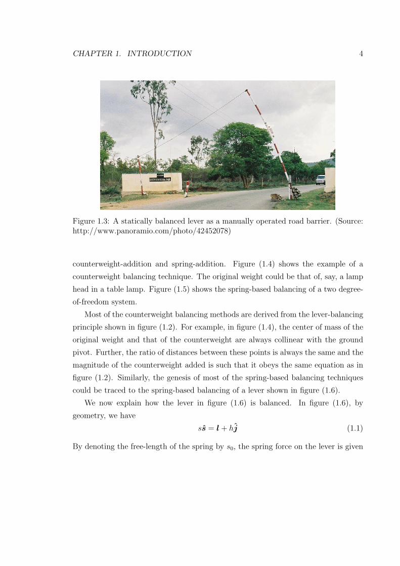
Figure 1.3: A statically balanced lever as a manually operated road barrier. (Source:http://www.panoramio.com/photo/42452078)
counterweight-addition and spring-addition. Figure (1.4) shows the example of a
counterweight balancing technique. The original weight could be that of, say, a lamp
head in a table lamp. Figure (1.5) shows the spring-based balancing of a two degree-
of-freedom system.
Most of the counterweight balancing methods are derived from the lever-balancing
principle shown in figure (1.2). For example, in figure (1.4), the center of mass of the
original weight and that of the counterweight are always collinear with the ground
pivot. Further, the ratio of distances between these points is always the same and the
magnitude of the counterweight added is such that it obeys the same equation as in
figure (1.2). Similarly, the genesis of most of the spring-based balancing techniques
could be traced to the spring-based balancing of a lever shown in figure (1.6).
We now explain how the lever in figure (1.6) is balanced. In figure (1.6), by
geometry, we have
ss = l + hj (1.1)
By denoting the free-length of the spring by s0, the spring force on the lever is given

CHAPTER 1. INTRODUCTION 5
Counter weight
Original weight
Figure 1.4: Counterweight balancing in a two degree-of-freedom linkage
Original weight
Figure 1.5: Spring-based balancing in a two degree-of-freedom linkage
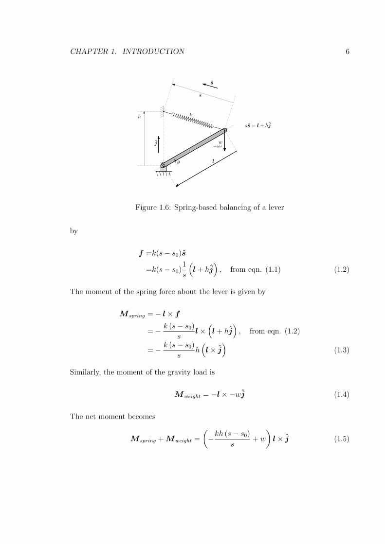
CHAPTER 1. INTRODUCTION 6
θ l
kh
wweight
j
s
ss = l + hj
s
Figure 1.6: Spring-based balancing of a lever
by
f =k(s− s0)s
=k(s− s0)1
s
(
l + hj)
, from eqn. (1.1) (1.2)
The moment of the spring force about the lever is given by
M spring =− l× f
=−k (s− s0)
sl×(
l + hj)
, from eqn. (1.2)
=−k (s− s0)
sh(
l× j)
(1.3)
Similarly, the moment of the gravity load is
Mweight = −l×−wj (1.4)
The net moment becomes
M spring +Mweight =
(
−kh (s− s0)
s+ w
)
l× j (1.5)
CHAPTER 1. INTRODUCTION 7
If we want static balance, then the net moment has to be zero over a continuous range
of θ. Given that l × j is zero at only discrete values of theta, we can only expect its
coefficient to be zero over a continuous set of configurations. However, when s0 6= 0,
the coefficient could become zero, again, at only a discrete set of configurations (Note
that s is a function of θ). Nevertheless, if we can have s0 = 0, i.e., if we can have a
spring of zero free-length, then the coefficient becomes a constant over every θ and,
in particular, zero if kh = w. Thus, the conditions under which the lever shown in
figure (1.6) attains static balance are zero free-length and kh = w. While achieving
kh = w is not hard, it is not popularly known that zero-free-length can also be
achieved in practice. The credit for recognizing the importance of zero free-length in
static balance and also its practical implementation goes to George Carwardine [2]
and Lucien LaCoste [3].
Having understood the necessity of zero-free-length springs for perfect static bal-
ance, we now focus on one of the ways of its practical realization. Figure (1.7) shows
the spring force (f) versus the relative distance (d) of anchor points of a linear ex-
tension spring for various cases. The plot for zero-free-length spring is expected to
be collinear with the origin, as shown in figure (1.7a). A normal extension spring
not only has a finite positive free-length but also what is called as pre-tension. In a
pre-tensioned spring, even if there is no external force, the coils press against each
other. The coils separate and the spring extends only when the external force is more
than the pre-tension. The effect of free-length l0 is to shift the force-distance plot
along l axis by l0 and the effect of pre-tension fp is to shift the plot along the f -axis
by fp. When fp is kl0 where k is slope of the plot (i.e., the stiffness of the spring), the
plot becomes collinear with the origin. Thus, even with unavoidable free-length, by
inducing appropriate pre-tension, one can have force-distance relation to be the same
as that of a zero-free-length spring for l > l0. Therefore, there is no practical hin-
drance in realizing a zero-free-length spring. There are several other ways of realizing
a zero-free-length spring, as discussed in [4] and [5].

CHAPTER 1. INTRODUCTION 8
l0
fp
l
f
l
f
l0l
f(force)
(distance)
(a) zero free length(b) positive free length without
pre-tension
(c) positive free length with pre-tension
Figure 1.7: Effects of free-length and pre-tension on force-distance plot of a linearextension spring

CHAPTER 1. INTRODUCTION 9
1.1.2 Compliant mechanisms and its static balance
In recent years, compliant mechanisms have emerged as a plausible design option,
especially in micro mechanical systems. A compliant mechanism, in contrast to a
rigid-body linkage, is made up of a single monolithic piece that transmits force and
displacement through elastic deformation. They are quite amenable to microfabrica-
tion techniques apart from being free of friction and backlash.
Analysis of rigid-body mechanisms can often be carried out analytically. This is
possible since it is the geometry of triangles, quadrilaterals and other polygons that
underlies the kinematics of rigid-body mechanisms. Furthermore, many graphical and
analytical synthesis methods have also been developed for the design of rigid-body
linkages. Accurate analysis of compliant mechanisms, on the other hand, generally
require numerical finite element analysis.
In an attempt to bring the analytical and graphical techniques developed for the
synthesis of rigid-body mechanisms into the realm compliant mechanisms, Midha and
Howell ([6], [7]) developed pseudo-rigid-body model for a class of compliant mecha-
nisms. This model allows a certain class of compliant mechanisms to be approximately
represented by spring-loaded rigid-body mechanisms. Flexure-based compliant mech-
anism form an important subclass of compliant mechanisms that can be represented as
spring-loaded rigid-body mechanisms. Howell and Midha [7] showed that the flexure
can be approximated by a revolute joint with a torsional spring having linear torque–
angle characteristics. This type of approximation is popularly know as small-length
flexure approximation. Thus, with these models, one can bring in several analytical
and graphical rigid-body mechanism design techniques into the realm of compliant
mechanisms.
Static balance of compliant mechanisms
While compliant mechanisms are superior to rigid-body mechanisms in terms of fric-
tion and backlash, they have a feature that could be disadvantageous. Figure (1.8
a) shows a compliant mechanism. Figure (1.8 b) shows the mechanism acting on a
workpiece. Figure (1.8 c) shows the same mechanism requiring effort even though it

CHAPTER 1. INTRODUCTION 10
is not acting on any workpiece. Mere actuation of the compliant mechanism requires
effort. The source of this effort is due to the spring-like behaviour of the compliant
mechanism arising out of its inherent elasticity.
(a)
(b) (c)
Figure 1.8: A compliant crimper
Statically balancing the elastic forces, i.e., nullifying the spring-like behaviour of
compliant mechanisms is under increasing attention. The reason for that is not just
the reduction in the effort to operate a compliant mechanism but also the prospect

CHAPTER 1. INTRODUCTION 11
of having tools that offer good force feedback. If a person handling a tool gets a good
sense of the force that the tool is applying on a workpiece, then the tool is said to
offer good force feedback. In certain tools consisting of linkages, such as laparoscopic
grippers, the force feedback is very bad for the reasons attributed to friction in the
joints. Compliant mechanisms on the other hand do not have joint-friction but their
spring-like behaviour can affect the force feedback. If this spring-like behaviour can
be removed, then compliant mechanisms can offer good force feedback.
1.1.3 Static balance: rigid-body linkage vs. compliant mech-
anisms
In rigid-body linkages, for static balance, we often want all possible motion that
the linkage can take to be effortless. This implies that conservative forces in all its
configurations are in equilibrium. As per our definition, “all possible motion” is not
necessary to qualify as static balance. Nevertheless, in this thesis, to comply with the
popular notion, we have struck to this “all possible motion” as far as static balancing
of rigid-body linkages are concerned.
In compliant mechanisms, which have infinite degree-of-freedom, in contrast to
finite degree-of-freedom of rigid-body linkages, it is not feasible to expect all possible
motion to be effortless. Only one or two modes of motion (or deformation) in which
the compliant mechanism normally operates is sought to be made effortless. In other
words, we aim to make configurations only along one or two paths to be in equilibrium.
1.2 Motivation for the thesis
The motivating idea of this thesis is to make use of rigid-body approximations, such
as pseudo-rigid-body model, for static balancing of compliant mechanisms. This mo-
tivation was first proposed in [8]. Pseudo-rigid-body model was successful in the
synthesis of compliant mechanisms because of the existence of simple analytical tech-
niques for the synthesis of rigid-body mechanisms. Similarly, for pseudo-rigid-body
model to be successful in making statically balanced compliant mechanisms, there
CHAPTER 1. INTRODUCTION 12
has to be simple analytical techniques for static balancing of spring-loaded linkages
rather than gravity-loaded linkages.
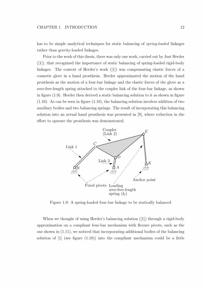
Prior to the work of this thesis, there was only one work, carried out by Just Herder
([1]), that recognized the importance of static balancing of spring-loaded rigid-body
linkages. The context of Herder’s work ([1]) was compensating elastic forces of a
cosmetic glove in a hand prosthesis. Herder approximated the motion of the hand
prosthesis as the motion of a four-bar linkage and the elastic forces of the glove as a
zero-free-length spring attached to the coupler link of the four-bar linkage, as shown
in figure (1.9). Herder then derived a static balancing solution to it as shown in figure
(1.10). As can be seen in figure (1.10), the balancing solution involves addition of two
auxiliary bodies and two balancing springs. The result of incorporating this balancing
solution into an actual hand prosthesis was presented in [9], where reduction in the
effort to operate the prosthesis was demonstrated.
Loadingzero-free-lengthspring (kl)
AB
C
D
K
Coupler(Link 2)
Link 3
Link 1
E
Fixed pivots
Anchor point
Figure 1.9: A spring-loaded four-bar linkage to be statically balanced
When we thought of using Herder’s balancing solution ([1]) through a rigid-body
approximation on a compliant four-bar mechanism with flexure pivots, such as the
one shown in (1.11), we noticed that incorporating additional bodies of the balancing
solution of [1] (see figure (1.10)) into the compliant mechanism could be a little

CHAPTER 1. INTRODUCTION 13
AK
kl
E
DF T
B
H
kb
C
Auxiliary links
G
Balancing spring 1
Balancing spring 2
Loading springkt
Anchor point
Anchor point
Figure 1.10: A static balancing solution for the spring-loaded four-bar linkage byaddition of auxiliary links and springs
cumbersome. This motivated us to take a closer look at the principles of static
balancing to see if there are other ways of statically balancing the same spring-loaded
four-bar linkage (of figure (1.9)), preferably, without using auxiliary bodies. We did
find other ways of balancing the four-bar linkage and one such way does not use
auxiliary bodies. We could also get some new general static balancing techniques
without using auxiliary bodies. We eventually gave a framework for making use of
these static balancing solutions to make statically balanced flexure-based compliant
mechanisms through small-length flexure model. An overview of these contributions,
which make up the bulk of the chapters in the thesis is presented next.
CHAPTER 1. INTRODUCTION 14
R
Figure 1.11: A compliant four-bar mechanism
1.3 Scope of the thesis
1.3.1 Three methods to statically balance a zero-free-length
spring-loaded four-bar linkage
For the static balancing problem shown in figure (1.9), apart from the method shown
in figure (1.10), which was already in the literature [1], we give two more methods
where the number of additional springs and the number of auxiliary links are less than
or equal to that of the method shown in figure (1.10). Further, we also recognized a
variant of the method given in figure (1.10). Among the methods that we give, one
method does not use any auxiliary link. These results are elaborated in Chapter 3.
1.3.2 Static balancing of cognates
In kinematics, there is a well-known theorem called Roberts-Chebyshev cognate the-
orem (see [10], for example). According to the theorem, for every four-bar linkage
with a specified coupler point on it, one can find two more four-bar linkages and
coupler points on them such that the coupler curves of the three four-bar linkages
are the same. These three four-bar linkages are termed as cognates. The triangle

CHAPTER 1. INTRODUCTION 15
formed by the ground anchor points of cognates, called the cognate triangle, plays a
central role in a few other elegant relations that the theorem states. With the intent
to extend the theorem to static balancing, we present some relations among static
balancing parameters (spring constants and anchor points of balancing springs) of
different cognates in which the cognate triangle again plays a central role. These
results are elaborated in Chapter 4.
1.3.3 Static balancing of revolute-jointed linkages without
auxiliary links
Building upon a method discussed in Section 1.3.1, we present a general method
that can statically balance any revolute-jointed linkage having zero-free-length spring
force and constant force interactions between the bodies constituting the linkage.
This method adds only zero-free-length springs but not auxiliary links. This result is
elaborated in Chapter 5.
1.3.4 Static balancing of spatial and/or revolute jointed link-
ages without auxiliary links
Further extending the planar method of Section 1.3.3 to spatial linkages, we show that
any spatial revolute and/or spherical jointed linkages with zero-free-length spring and
constant force interactions can be statically balanced. Again, the method of balancing
requires only addition of zero-free-length springs but not auxiliary links. This result
is elaborated in Chapter 6.
1.3.5 Static balancing of flexure-based compliant mecha-
nisms by addition of springs
As pointed in Section 1.2, the motivation to find new methods for static balancing of
spring-loaded rigid-body linkages was to make statically balanced compliant mecha-
nisms through pseudo-rigid-body model. Having found the new methods, we give a

CHAPTER 1. INTRODUCTION 16
simple step-by-step framework for static balancing of a flexure-based compliant mech-
anisms through small-length flexure model. We give four examples to illustrate the
framework. A prototype of one of the examples is also made. Both simulations and
the fabricated prototype show more than 70 % reduction in the effort. These results
are described in Chapter 7.
Summary
• Static balance implies equilibrium among conservative forces over a continuous
set of configurations.
• Static balancing of rigid-body mechanisms generally focus on compensating
gravity forces.
• Primary focus in static balancing of a compliant mechanism is to compensate
the inherent elastic forces of the compliant mechanism.
• The motivating idea of the thesis is to use rigid-body models of compliant
mechanisms to design statically balanced compliant mechanisms. We recognize
that for the idea to be successful, it is necessary to have new analytical static
balancing methods for spring-loaded rigid-body linkages.
• This thesis presents new static balancing methods for spring-loaded linkages
without using auxiliary bodies. The thesis also presents a simple framework to
use these methods through small-length flexure model for static balancing of
compliant mechanisms.
• The last section of this chapter defined the scope of the thesis and its organi-
zation in the remaining chapters.
Chapter 2
Literature Survey
Overview
• Literature on static balancing of gravity-loaded rigid-body linkages by adding
counter-weights or springs.
• Literature on the importance of static balancing of spring-loaded rigid-body
linkages and the existing methods to handle such problems.
• Literature on various approaches that have been pursued to address the design
of statically balanced compliant mechanisms.
2.1 Rigid-body linkages under gravity loads
There are two dominant ways of balancing a linkage under gravity loads. One is by
addition of counter weights and the other is by addition of springs. The literature in
these fields is described next.
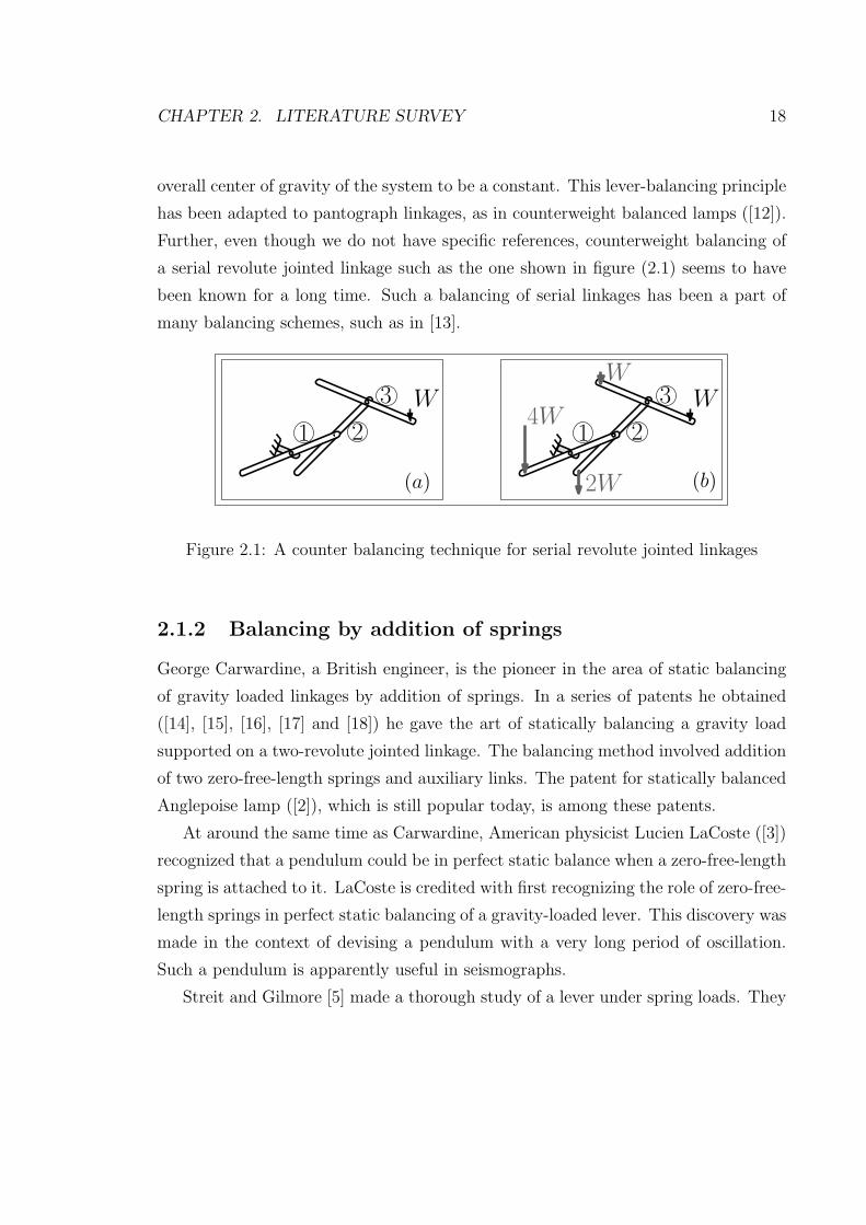
2.1.1 Counter-weight balancing
The simplest of rigid-body linkages is a lever. The conditions for static balance of a
lever under gravity loads was first given by Archimedes ([11]). It relies on making the
17
CHAPTER 2. LITERATURE SURVEY 18
overall center of gravity of the system to be a constant. This lever-balancing principle
has been adapted to pantograph linkages, as in counterweight balanced lamps ([12]).
Further, even though we do not have specific references, counterweight balancing of
a serial revolute jointed linkage such as the one shown in figure (2.1) seems to have
been known for a long time. Such a balancing of serial linkages has been a part of
many balancing schemes, such as in [13].
W
1 2
3 W
W
2W
4W1 2
3
(a) (b)
Figure 2.1: A counter balancing technique for serial revolute jointed linkages
2.1.2 Balancing by addition of springs
George Carwardine, a British engineer, is the pioneer in the area of static balancing
of gravity loaded linkages by addition of springs. In a series of patents he obtained
([14], [15], [16], [17] and [18]) he gave the art of statically balancing a gravity load
supported on a two-revolute jointed linkage. The balancing method involved addition
of two zero-free-length springs and auxiliary links. The patent for statically balanced
Anglepoise lamp ([2]), which is still popular today, is among these patents.
At around the same time as Carwardine, American physicist Lucien LaCoste ([3])
recognized that a pendulum could be in perfect static balance when a zero-free-length
spring is attached to it. LaCoste is credited with first recognizing the role of zero-free-
length springs in perfect static balancing of a gravity-loaded lever. This discovery was
made in the context of devising a pendulum with a very long period of oscillation.
Such a pendulum is apparently useful in seismographs.
Streit and Gilmore [5] made a thorough study of a lever under spring loads. They

CHAPTER 2. LITERATURE SURVEY 19
discussed achieving a set of discrete as well as a set of continuous equilibrium config-
urations. Some of the ways to realize zero-free-length springs were also discussed.
Nathan [19] gave a way to extend the spring-based lever-balancing to two-degree-
of-freedom linkages using auxiliary parallelogram linkages. Pracht et al. [20] made
a slightly different extension where all the springs are anchored from the ground to
different parts of the linkage. Streit and Shin [21] made another extension using
pantograph linkages. They obtained different design variants by varying input points
and input motion. They also suggested that such a gravity-balancer could be used
in walking machines so that the torque requirement of the motors is reduced. The
attempt of Wongrathanaphisan and Cole [22] to statically balance a load on the
coupler of a four-bar linkage led to a solution that is conceptually not different from
LaCoste’s solution.
Nathan [19] also extended his two-degree-of-freedom linkage-balancing to a n-
degree-of-freedom revolute-jointed linkage. Figure (2.2) illustrates the method in [19]
where, to balance a gravity load on a 3R linkage shown in figure (2.2a), auxiliary
linkages (colored in grey) and extra springs are added. Streit and Shin [23] similarly
extended the work of Pracht et al. [20] to a n-degree-of-freedom revolute-jointed
linkage. Reference [23] termed the extension of Nathan [19] as “vertical link systems”
and their extension of reference [20] as “parallel link systems”. It also presented static
balancing of a linkage having a series of revolute-prismatic pairs of joints.
WW
1 2
3
(a) (b)
Figure 2.2: Use of auxiliary links (colored in grey) along with springs in an existingtechnique for balancing a n-degree-of-freedom linkage under constant load.

CHAPTER 2. LITERATURE SURVEY 20
Herder’s PhD thesis [4] brought new approaches to the field of spring-based static
balancing. Herder obtained a variety of multi-degree-of-freedom gravity-balancing
linkages using 1) a few modification rules, 2) a few basic statically balanced linkages,
such as the balanced lever of LaCoste, and 3) the properties of auxiliary parallelogram
and pantograph linkages. Herder also introduced the concept of a floating suspension.
Whatever reaction forces that a pivot exerts on a gravity-loaded lever, the same forces
could be exerted by a floating suspension, which is nothing but springs anchored from
the ground to the lever. Thus, under quasi-static conditions, a floating suspension
could form a friction-less replacement for a pivot.
Walsh et al. [24] showed a way to balance a spatial rigid-body attached to the
ground by a two degree-of-freedom joint formed by two revolute joints of intersecting
axes. Streit et al. [25]), in a similar work, dealt with two degree-of-freedom Hooke’s
joint in a somewhat different way. Wongratanaphisan and Chew [26] gave a way to
balance a more general revolute-jointed two-degree-of-freedom serial spatial manipu-
lator using auxiliary links. Agrawal and Fattah [27] provided an interesting method
to balance a spatial gravity-loaded linkage. In the method, by adding auxiliary paral-
lelogram linkages, a physical point that is also the center of mass of the overall system
is first identified. Then, depending on the kind of motion this center of mass under-
goes, springs are added to compensate the gravity. The work of Rahman et al. [28]
gives a straight forward extension of Nathan’s “vertical link systems” to spatial n–
body revolute-jointed linkages. While Rahman et al. [28] used simple parallelograms
in their extension, Lin et al. [29] used spatial RSSR (revolute-spherical-spherical-
revolute) parallelogram linkages to provide a more comprehensive extension. There
is a lot of literature on the static balancing of parallel manipulators such as [13], [30],
[31], [32], [33], [34], [35], [36], [37] and [38].
While the techniques in the above literature use auxiliary bodies in addition to
springs, we (Sangamesh and Ananthasuresh [39]) showed how to balance a n-degree-
of-freedom (n ≥ 1) revolute-jointed spring and/or gravity linkage using only springs
but not auxiliary bodies. Lin et al. [40], using what they called as stiffness matrix
approach, also provided balancing methods without auxiliary bodies for two and three
revolute-jointed serial gravity-loaded linkages. Shieh and Chen [41] showed how to
CHAPTER 2. LITERATURE SURVEY 21
statically balance revolute-jointed planar one-degree-of-freedom closed-loop linkages
without using auxiliary links. Our work [39] was extended in [42], which gave more
general static balancing conditions.
All the techniques discussed above use zero-free-length springs for perfect static
balance of the gravity loads. While there are a few works that use other kinds of
springs as balancing elements, they are either approximate balancing techniques or use
cams to modulate the spring behaviour. Gopalswamy et al. [43] gave an approximate
static balancing technique where torsional springs are used as balancing elements.
Agrawal and Agrawal [44] presented an approximate static balancing method using
non-zero-free-length springs. The balancing techniques that modulate the behaviour
of springs include the technique in [45], where a pulley of varying radius was used,
and the technique in [46] and [47], where a cam was used.
There are a few works dealing with biomedical applications of static balancing.
The ones dealing with leg include [48], [49], [50], [51], [52], [53], [54], [55], and [56].
The ones that deal with upper limb include [57], [58], [59], [60], [61], [62] and [63].
2.2 Rigid linkages under spring loads
Herder’s work [1] was the first to recognize the importance of a class of problems where
springs forces, which could be an approximation for more complex elastic forces, need
to be compensated. The motivation for the work was to compensate the elastic forces
of the cosmetic glove of a hand prosthesis. In this work, the motion of the fingers of a
hand prosthesis was modelled as the motion of the coupler link of a four-bar linkage.
The elastic forces of the cosmetic glove were lumped into to a zero-free-length spring
attached to a point on the coupler. The work then gives a perfect balancing solution
for statically balancing this spring-loaded four-bar linkage. The obtained solution is
based on extending the balancing of a skew lever to a skew pantograph. Incorporation
of the pantograph results in auxiliary bodies being added to the four-bar linkage.
Visser and Herder [9] used the solution of [1] in an actual hand prosthesis and gave
quantitative data on the reduction of effort in actuation of the fingers.
CHAPTER 2. LITERATURE SURVEY 22
Our work [8] was the first to recognize that the compensation methods for spring-
loaded linkages are useful in approximately compensating flexure-based compliant
mechanisms as well. The recognition was based on small-length flexure model [64]
where flexure-based compliant mechanisms could be replaced by rigid-body linkages
under torsional-spring loads. The recognition was also the motivation for our work [8]
where we found that a larger set of methods can address the problem of spring-force
compensation enunciated in [1].
One of the methods in [8] led us to a more general class of spring-force compen-
sation methods [39]. Reference [39] showed that any n-rigid-body linkage under zero-
free-length spring and/or constant force can be compensated by addition of springs.
This method does not require addition of auxiliary bodies. The same method was
generalized and also presented in a more systematic manner in [42]. In [42], we ar-
gued that the method is applicable not only for planar linkages but also for spatial
linkages.
The small-length flexure model gives a rigid-body linkage loaded with torsional
springs. Hence, it may seem natural that there be a focus on finding static balancing
methods for rigid-body linkages loaded with torsional springs rather than extension
springs, as in [1], [8], [39] and [42]. However, our own attempts at finding an analyt-
ical solution to static balancing of torsional spring-loaded linkages did not yield any
results. A similar attempt by Radaelli et al. [65] relies on genetic-algorithm-based
numerical optimization or a manual search. To facilitate the manual search, which
could potentially give some insights, they developed an interactive interface called
“interactiveparams”. In, this thesis, we however approximate the torsional springs
by zero-free-length springs through matching a few terms in the Taylor series expan-
sion and then continue to use the analytical methods for balancing zero-free-length
spring-loaded linkages.
2.3 Static balance of compliant mechanisms
One of the earliest papers that recognized the importance of statically balanced com-
pliant mechanisms is [66]. Design of laparoscopic graspers that can give good force

CHAPTER 2. LITERATURE SURVEY 23
feedback to the operator has been the main motivation in the field of statically bal-
anced compliant mechanisms. The papers that specifically focussed on laparoscopic
graspers include [67], [68] and [69]. Stapel and Herder [67] showed that a fully com-
pliant, statically balanced grasper is feasible. Tolou and Herder [68] separated a
statically balanced compliant grasper into grasper part and balancer part. They fo-
cused on obtaining a negative stiffness balancer that can compensate the positive
stiffness of compliant grasper. De Lange et al. [70] also used the concept of grasper
and balancer. They used topology optimization to match the stiffness characteristics
of a grasper and a balancer.
Various synthesis strategies for statically balanced compliant mechanisms, not re-
stricted to just graspers, has been addressed in [71], [72] and [73]. Morsch and Herder
[71] gave a compliant joint that is statically balanced so that when a linkage is built
out of these compliant joints, the linkage would be in static balance. Building block
approach is one of the known strategies in the synthesis of compliant mechanisms
and Hoetmer et al. [72] explored its extension to static balancing. Rosenberg et al.
[73] made use of the results of Radaelli et al. [65] to design flexure-based statically
balanced compliant mechanisms.
Research in static balance has ventured in tensegrity structures well, as could be
seen in [74] and [75]. The work of Guest et al. [76] where they present a zero-stiff
elastic shell is worth taking note of.
2.4 Prior Art
Prior to our work, the work in [1] was the only work that dealt with analytical solution
to static balancing of a spring-loaded rigid-body linkage. We now describe the way
the solution was arrived at in [1] along with necessary preliminaries that can also be
found in [4].

CHAPTER 2. LITERATURE SURVEY 24
2.4.1 Preliminaries
Statically balanced lever under spring loads
Consider a lever under the action of two zero-free-length springs, as shown in figure
(2.3). The spring on the left hand side is anchored between points D and P . Let the
spring force on the lever at D be a positive constant times the relative displacement
of point P with respect to D, i.e., k1−−→DP . Similarly, the spring force due to right hand
spring is k2−−→DN . Let these forces be resolved along
−−→DA and
−−→PN . When the constants
and anchor points are chosen such that k1−→AP = −k2
−−→AN , the resolved forces along
−−→PN become zero and the remnant forces along
−−→DA gives zero moment on the lever
about A. This signifies equilibrium. Moreover, this is true for any configuration of
the lever. Hence, we have static balance here.
ANP
k2k1
k2−−→
AN
k2−−→
DAk1−−→
DA
k1−→
AP
Dφ
Figure 2.3: A basic spring force balancer
To appreciate the critical role played by zero-free-length of the springs, consider
a case where the free-length of the spring is not zero. Then, the spring force on D
from A is actuallyl1−l01
l1
−−→DA where l01 is the free-length and l1 is the relative distance
of the anchor points. The resolved components of the forces are as shown in figure
(2.4). Similarly, the resolved components of the right hand side spring are also shown.
It may be noted that no matter what strictly positive values l01 , k1, l02 and k2 take
and where P and N are placed, the resolved forces along−−→PN cannot cancel at every
configuration. The contrast between figures (2.3) and (2.4) in terms of static balance
should highlight the necessity of zero-free-length character for perfect static balance.

CHAPTER 2. LITERATURE SURVEY 25
ANP
k2k1
l1 − l01
l1k1
−→
AP
Dφ
l1 − l01
l1k1
−−→
DA l2 − l02
l2k2
−−→
DA
l2 − l02
l2k2
−−→
AN
l1 = PD
l2 = ND
Figure 2.4: A lever with ordinary springs
Statically balanced parallelogram linkage
Figure (2.5) shows a parallelogram linkage, ADEN , with two springs attached diago-
nally between the joints. It may be verified that, for the same φ, the potential energy
of this system is the same as that in figure (2.3). If one is statically balanced, so is
the other.
N
D
Aφ
kk
E
Figure 2.5: Balanced parallelogram
Figure (2.6) shows again a parallelogram linkage that now has two degrees of
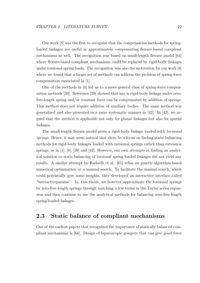
freedom. For the same φ, the potential energy of this system is the same as that in
CHAPTER 2. LITERATURE SURVEY 26
figure (2.5). If one is statically balanced, so is the other.
A
N
E
Dφ
k
k
θ
Figure 2.6: Balanced two degree-of-freedom parallelogram linkage
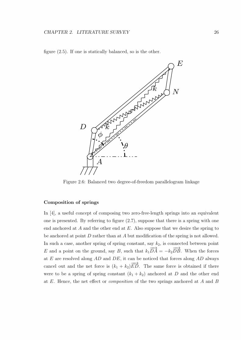
Composition of springs
In [4], a useful concept of composing two zero-free-length springs into an equivalent
one is presented. By referring to figure (2.7), suppose that there is a spring with one
end anchored at A and the other end at E. Also suppose that we desire the spring to
be anchored at point D rather than at A but modification of the spring is not allowed.
In such a case, another spring of spring constant, say k2, is connected between point
E and a point on the ground, say B, such that k1−−→DA = −k2
−−→DB. When the forces
at E are resolved along AD and DE, it can be noticed that forces along AD always
cancel out and the net force is (k1 + k2)−−→ED. The same force is obtained if there
were to be a spring of spring constant (k1 + k2) anchored at D and the other end
at E. Hence, the net effect or composition of the two springs anchored at A and B

CHAPTER 2. LITERATURE SURVEY 27
is a virtual spring anchored at D. This is an important concept for the techniques
presented in this chapter.
A B
D
E
k1 k2
k1−−→DA = −k2
−−→DB
k2−−→ED
k2−−→DB
k1−−→ED
k1−−→DA
Figure 2.7: Composition of two zero-length-spring into an equivalent one. The virtual,equivalent spring between E and D is shown in grey color.
2.4.2 Plagiograph
In a plagiograph linkage, the path traced at the output point is a scaled and rotated
replica of the path traced at the input point. If the linkage shown in figure (2.8)
satisfies the following conditions:
Condition 1: PQ = SR and PS = QR so that PQRS is a parallelogram,
Condition 2: ∠RQM = ∠NSR (this angle is labelled as α) and RQ
MQ= NS
RS(this ratio is
labelled as m) so that △NSR is similar to △RQM ,
then the linkage is called a plagiograph and it can be proved to have the following
property: output point N follows the input point M through a scaling and rotation
transformation about point P with the scale factor and the rotation angle being m
and α. That is,−−→PN = mRα(
−−→PM) (2.1)
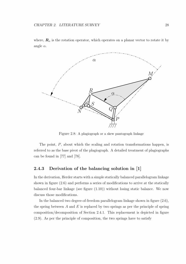
CHAPTER 2. LITERATURE SURVEY 28
where, Rα is the rotation operator, which operates on a planar vector to rotate it by
angle α.
M
S
α
α
P
α
Q
R
N
Figure 2.8: A plagiograph or a skew pantograph linkage
The point, P , about which the scaling and rotation transformations happen, is
referred to as the base pivot of the plagiograph. A detailed treatment of plagiographs
can be found in [77] and [78].
2.4.3 Derivation of the balancing solution in [1]
In the derivation, Herder starts with a simple statically balanced parallelogram linkage
shown in figure (2.6) and performs a series of modifications to arrive at the statically
balanced four-bar linkage (see figure (1.10)) without losing static balance. We now
discuss those modifications.
In the balanced two degree-of-freedom parallelogram linkage shown in figure (2.6),
the spring between A and E is replaced by two springs as per the principle of spring
composition/decomposition of Section 2.4.1. This replacement is depicted in figure
(2.9). As per the principle of composition, the two springs have to satisfy
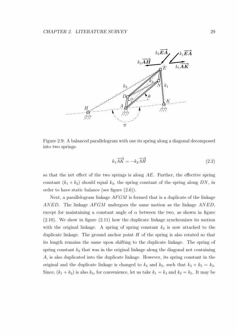
CHAPTER 2. LITERATURE SURVEY 29
AK
E
H
π
k1k2
k3
θφ
N
D
k1−−→
AK
k1
−→
EAk2
−→
EA
k2
−−→
AH
Figure 2.9: A balanced parallelogram with one its spring along a diagonal decomposedinto two springs.
k1−−→AK = −k2
−−→AH (2.2)
so that the net effect of the two springs is along AE. Further, the effective spring
constant (k1 + k2) should equal k3, the spring constant of the spring along DN , in
order to have static balance (see figure (2.6)).
Next, a parallelogram linkage AFGM is formed that is a duplicate of the linkage
ANED. The linkage AFGM undergoes the same motion as the linkage ANED,
except for maintaining a constant angle of α between the two, as shown in figure
(2.10). We show in figure (2.11) how the duplicate linkage synchronizes its motion
with the original linkage. A spring of spring constant k2 is now attached to the
duplicate linkage. The ground anchor point H of the spring is also rotated so that
its length remains the same upon shifting to the duplicate linkage. The spring of
spring constant k3 that was in the original linkage along the diagonal not containing
A, is also duplicated into the duplicate linkage. However, its spring constant in the
original and the duplicate linkage is changed to k4 and k5, such that k4 + k5 = k3.
Since, (k1 + k2) is also k3, for convenience, let us take k1 = k4 and k2 = k5. It may be

CHAPTER 2. LITERATURE SURVEY 30
noted that the potential energy of the spring in figure (2.10) is the same as that in
figure (2.9). Hence, the static balance in figure (2.9) implies that the linkage of figure
(2.10) is also statically balanced. It may be noted that because of this step, equation
(2.2) gets modified to
k1Rα
(−−→AK
)
= −k2−−→AH (2.3)
where Rα is a rotation operator that rotates a vector by an angle α.
α
φθ K
E
k1
k4
k2
k5
A
H
G
k2
π − α
F N
D
M
Figure 2.10: The parallelogram linkage with a duplicate that maintains a constantangle of α from the original
Figure (2.11) shows how the parallelogram linkages ANED and AFGM can be
made to have the same motion except for maintaining a constant angle between
them. Here, essentially, a plagiograph has been introduced into the parallelogram
linkages. The following conditions have to be satisfied to have the synchronized
motion: ED = DC, ∠EDC = α, CF = FG, ∠CFG = α.
The parallelogram linkage AFGM is scaled by a factor of m, about point A, as
shown in figure (2.12). The plagiograph that maintains the synchronization between

CHAPTER 2. LITERATURE SURVEY 31
α
αα
K
E
k1
k4
k2
k5
A
H
k2
π − α
N
D
M
F
C
G
Figure 2.11: Synchronization of motion between two parallelogram linkages
the two parallelogram linkages gets modified accordingly, as shown in the figure. The
two springs attached to it are also scaled by the same factor. This necessitates that
the anchor point H be also scaled by the same factor about A. Because of the
spatial scaling, the potential energy of the two springs scales by the square of the
scaling factor m. To restore the potential energy to that of figure (2.11), the spring
constants of the two springs are scaled by a factor of 1/m2. Since the potential energies
in figure (2.11) and (2.12) are the same, the static balance in figure (2.11) implies
the static balance in figure (2.12) too. Because of these modifications, equation (2.3)
gets modified to
k1Rα
(−−→AK
)
= −m2k21
m
−−→AH = −mk2
−−→AH (2.4)
As far as the length is concerned, the spring between M and F is an exact replica
of the spring between D and N , except for a scale factor m. Hence, one can elim-
inate the spring between D and N and increase the stiffness of the spring between
M and F from k2 to (k2 + k1/m2) so that the potential energy remains unaltered.

CHAPTER 2. LITERATURE SURVEY 32
N
E
D
C
F
M
H
G
α
k1
k2
π − α
KA
α
α
k5 = k2
k4 = k1
Figure 2.12: Scaling the duplicate parallelogram linkage
This alteration is shown in figure (2.13) where two links AN and NE are no longer
necessary. Again, static balance has remained unaltered due to unaltered potential
energy.
As shown in figure (2.14), two more links AM and MG can also be removed by
relocating the spring between M and F to be between A and T where T is a point
on link GFC such that−→GF =
−→FT . Since MF = AT , this relocation does not change
the potential energy. Hence, the static balance remains intact. Again, adding a link
BC, as shown in the same figure does not disturb the static balance. The intent of
this addition is to make the four-bar linkage BCDA. This is how the static balancing
solution given in figure (1.10) was arrived at in [4]. In this thesis, we take a different
approach to arrive at a static balancing solution to the spring loaded four-bar linkage,
leading to many more solutions. Further, we give a static balancing technique that is
applicable to general n-degree-of-freedom revolute and/or spherical jointed linkages.

CHAPTER 2. LITERATURE SURVEY 33
E
D
C
F
M
H
G
k1
k2
k5 = k2 + k1
m2
KA
π − α
α
α
Figure 2.13: Removal of a spring and compensating it with increase in stiffness ofanother spring
AK
kl
E
DF T
B
H
kb
C
Auxiliary links
G
Balancing spring 1
Balancing spring 2
Loading springkt
Anchor point
Anchor point
Figure 2.14: Removal of two more links.
CHAPTER 2. LITERATURE SURVEY 34
Summary
• There is a wide array of literature on static balancing of gravity-loaded rigid-
body linkages by addition of counter-weights as well as springs.
• Prior to our work, Herder’s derivation has been the only work in the area of
static balancing of spring-loaded linkages.
• Herder’s derivation is based on cascading modification of simple statically bal-
anced mechanism into the final mechanism without losing static balance in any
of the modifications.
• Literature shows that some of the strategies explored for designing statically bal-
anced compliant mechanisms include topology optimization, designing generic
zero-stiffness compliant joint and the building block approach.
Apart from Chapter 7, the bulk of the thesis is based on our work presented in [8]
and [42]. Hence, it may be apt to pictorially summarize our work and the literature
in a way that brings out the distinct features of our work. Figure (2.15) shows one
such representation.

CHAPTER 2. LITERATURE SURVEY 35
Rigid linkages
under
gravity load
By
addition
of mass
Rigid linkages
under
spring load
Compliant
mechanism
By
addition
of springs
Approximate
balancing
and
cam using
methods
Perfect
balancing
methods
Gopalswamy et al. (1992)
Agrawal & Agrawal (2005)
Ulrich & Kumar (1991)
Koser (2009)
For
specific
linkages
For
‘n’ - dof
linkages
LaCoste (1934)
Shin & Streit (1991)
Walsh et al. (1991)
Herder (2001)
Lin et al. (2010)
Using
auxiliary
bodies
Without
auxiliary
bodies
Streit & Shin (1993)
Agrawal & Fattah (2004)For planar revolutejointed and spatialrevolute and/orspherical jointedlinkages
Torsion
load
balanced
by
torsion
loads
Extension
spring
balanced
by
extension
springs
Approximate
methods
Perfect
methods
Radaelli et al. (2011)
For
specific
linkages
For
‘n’ -dof
linkages
Basic spring forcebalancer (Herder(2001))
Herder (1998)
Without
auxiliary
bodies
For planar revolutejointed and spatialrevolute and/orspherical jointedlinkages
Deepak & Ananthasuresh (2012)
Limiting case
By
addition
of springs
Other
strategies
Chapter 7 :Extension ofDeepak & Anan-thasuresh (2012)to compliantmechanisms usingpseudo-rigid bodymodel
Topology optimiza-tion (see De Lange etal. (2008))
Building block ap-proach (see Hoet-mer, et al. (2010))
Extension ofRadaelli et al.(2011) to compliantmechanisms as seenin Rosenberg et al(2011)
Original or novel contribu-
tions of this thesisdof: degree of freedom
Figure 2.15: The current literature and our contributions

Chapter 3
Static balancing of a four-bar
linkage loaded by a spring
Overview
• Static balancing of a spring-loaded four-bar linkage by incorporating a parallel-
ogram linkage.
• Static balancing without auxiliary bodies.
• Static balancing with the incorporation of a plagiograph linkage.
• A prototype demonstrating static balancing without auxiliary bodies.
3.1 Introduction
The problem that is addressed in this chapter is static balancing of a four-bar linkage
loaded with a zero-free-length spring connected between its coupler point and a point
on the ground. Figure (3.1) shows one such four-bar linkage. There is already one
method [1] whose derivation was discussed in detail in Section 2.4.3. The motivation
for attempting to find more methods, as discussed in the introduction, is to have a
suitable set of balancing methods that could be used in making statically balanced
36
CHAPTER 3. STATIC BALANCING OF A FOUR-BAR 37
compliant mechanisms using pseudo-rigid-body models. All the results of this chapter
are documented in our paper [8].
Loadingzero-free-lengthspring (kl)
AB
C
D
K
Coupler(Link 2)
Link 3
Link 1
E
Fixed pivots
Anchor point
Figure 3.1: A four-bar linkage with a zero-free-length spring anchored from its couplerto the ground
3.2 Static balancing of a given spring-loaded four-
bar linkage
Consider a four-bar linkage loaded by a zero-free length spring at its coupler point as
shown in figure (3.1). Before adding auxiliary links and balancing springs to balance
it, let us see if there is a possibility of it being in static balance as such. Figure (3.2)
shows the coupler curve traced by point E. If the linkage has to be in equilibrium
at every configuration, then the potential energy of the spring has to be the same at
every configuration. This is possible only when every point of the coupler curve is at
a constant distance from K, i.e., when the coupler curve is a circle centered at K. In

CHAPTER 3. STATIC BALANCING OF A FOUR-BAR 38
general this is not true except in extreme cases such as when E coincides with D (or
C) and K coincides with A (or B).
AB
C
D
K
E
kl
Figure 3.2: Possibility of the four-bar linkage being statically balanced as it is
Next, various possibilities of static balancing of a four-bar linkage are considered
by adding auxiliary links and springs. Only those possibilities where the number of
additional balancing springs and auxiliary links is less than or equal to that of [1]
are explained. As can be seen in figure (1.10), [1] used two auxiliary links and two
balancing springs.
3.2.1 Technique 1
Motivated by the observation in figure (2.6), the four-bar linkage can be balanced by
creating a balanced parallelogram as shown in figure (3.3). Here, four auxiliary links
and one balancing spring are used. But the number of auxiliary links can be reduced
to two as explained next.
Reducing the number of auxiliary links
As shown in figure (3.4), if T is a point on the (extended) link EP , such that−→EP =
−→PT , then TKQP forms a parallelogram. Relocation of the spring between P and Q
to be between T and K does not change its potential energy and hence static balance
is undisturbed. The advantage of the relocation is that the two auxiliary links KQ

CHAPTER 3. STATIC BALANCING OF A FOUR-BAR 39
AB
C
E
D
K
kl
kl
Q
P
Figure 3.3: A balanced parallelogram on the load spring
and QE are unnecessary. This way of balancing forms this chapter’s technique 1 to
statically balance a four-bar linkage.
AB
C
E
D kl
kl (balancing spring)
Q
T
P
K
l1 = PE
l2 = PKBalancing parameters
Figure 3.4: Technique 1: Static balancing with two auxiliary links and one balancingspring
The characteristics of technique 1 can be summarized as follows:
1. This way of balancing does not induce any stress in any of the links of the
four-bar linkage.

CHAPTER 3. STATIC BALANCING OF A FOUR-BAR 40
2. The balancing variables are l1 and l2, i.e., lengths of PE and PK, as shown in
figure (3.4). l1 and l2 can be of any convenient value.
3.2.2 Technique 2
Instead of adding four links to make up a parallelogram as in figure (3.3), if links ED
andDA are used to form the parallelogram as shown in figure (3.5), then two auxiliary
links can be avoided. This parallelogram can balance a spring connected between its
opposite vertices. While the load spring is not between its opposite vertices, another
spring (labelled as balancing spring 1) is added so that the resultant of its composition
with the load spring is between the opposite vertices of the parallelogram, as shown
in figure (3.6). Recall the composition property of springs noted in Section 2.4.1.
B
C
E
kl
F
D
A
K
Figure 3.5: Forming a parallelogram using two auxiliary links.
The virtual equivalent spring between A and E in figure (3.6) is balanced by
adding another spring (labelled as balancing spring 2) across the other two opposite
vertices of the parallelogram as shown in figure (3.7). Thus, the equivalent spring
and balancing spring 2 are in static balance. Equivalently, the load spring, balancing
spring 1 and balancing spring 2 are in static balance. With this, the linkage is in
static balance with two auxiliary links and two balancing springs. The auxiliary links
can be eliminated, as explained next.
As shown in figure (3.8), if T is a point on link DE (extended if necessary)
satisfying−−→ED =
−→DT , then AFDT is always a parallelogram and DF = TA. Hence,
CHAPTER 3. STATIC BALANCING OF A FOUR-BAR 41
B
kl
F
D
A
K
kb
−−→AH = kl
−−→KA, kt = kl + kb
kb
ktC
E
H
Balancing spring 1
Equivalent spring
Figure 3.6: A virtual spring between opposite vertices of the parallelogram AFED.
B
C
kl
K
kb
−−→AH = kl
−−→KA, kt = kl + kb
kb
E
F
HA
D
kt
Balancing spring 1
Balancing spring 2
Figure 3.7: Adding balancing spring 2 across opposite vertices of the parallelogramto balance the load spring and balancing spring 1.

CHAPTER 3. STATIC BALANCING OF A FOUR-BAR 42
relocation of the spring between D and F in figure (3.7) to be between T and A as
in figure (3.8), does not change its potential energy. Consequently, the static balance
is also undisturbed. Furthermore, auxiliary links AF and FE are no longer required.
This way of balancing shown in figure (3.8), requiring two balancing spring but no
auxiliary link, constitutes the second technique to balance a four-bar linkage.
B
C
E
kl
kb DK
kt
H
T
kb
−−→AH = kl
−−→KA, kt = kl + kb
−→TD =
−−→DE
A
F
Balancing spring 1
Balancing spring 2
Figure 3.8: Option 2 for balancing the four-bar linkage without requiring auxiliarylinks
This technique has two options. In figure (3.5), a parallelogram was completed
out of links AD and DE. One could have completed the parallelogram out of links
BC and CE as well and proceed in a similar manner. In the former case we say that
the balanced parallelogram is based at A and in the later case, it is based at B.
Among the balancing parameters of this technique, the anchor point of balancing
spring 2 is always one of the fixed pivots of the four-bar linkage. The remaining
balancing parameters: (i) H, the anchor point of balancing spring 1, (ii) kb, the
spring constant of balancing spring 1, and (iii) kt the spring constant of balancing
spring 2, have to be solved from equations included in figure (3.8). Those equations

CHAPTER 3. STATIC BALANCING OF A FOUR-BAR 43
can be rewritten in a general form so that they are applicable to both the options of
this technique. If W is where the balanced parallelogram is based (i.e., W is A or B)
and K is the anchor point of load spring, then
kb−−→WH = kl
−−→KW (3.1)
kb = klKWWH
(positive if−−→WH is along
−−→KW , and negative otherwise) (3.2)
kt = kb + kl (3.3)
Equation (3.1) says that H has to lie on a line starting fromW and along the direction
of−−→KW . The line is called the straight-line locus of H. Once a point on this line is
chosen as H, kb and kt get determined as per equations (3.2) and (3.3). Thus, the set
of solutions to (H, kb, kt) is a one-parameter family. This choice can be used to fulfill
practical considerations without compromising static balancing.
3.2.3 Technique 3
As mentioned earlier, the only known method in literature to statically balance a
spring-loaded four-bar linkage was described by [1]. In [1], a plagiograph is first
statically balanced and then it is modified to obtain balanced four-bar linkage with two
auxiliary links and two balancing springs as shown in figure (1.10). It is now shown
that the balancing arrangement obtained by [1] can also be obtained by combining
technique 2 of this chapter with the concept of plagiograph. Whereas this later
approach provides four options, the approach of [1] provides only two of these options.
The later approach constitutes the third technique of this chapter. The technique and
its options are described next.
In technique 2, the balancing spring 1 was connected to the same point as that
of the loading spring – the coupler point E. If the coupler point is not accessible to
the balancing spring 1, then another point to anchor the spring has to be found. It is
also desirable that the motion of the other point is related to the coupler point. By
taking a cue from Section 2.4.2, a plagiograph can be completed out of two links of
the given four-bar linkage, as shown in figure (3.9a) so that point G follows a scaled

CHAPTER 3. STATIC BALANCING OF A FOUR-BAR 44
and rotated locus of E.
}ADCF is a parallelogram
CDED
= GFCF
∠CFG = ∠EDC =⇒ △GFC ∼ △CDE
−→FT =
−→GF
kl
m2
−→LA = kb
−−→AH
kt = kl
m2 + kb
E
D
B
C
A
F
L
H
kb
G
Tkt
K
kl
E
D
B
C
A
F
L
H
kb
G
Tkt
−→FT =
−→GF
kl
m2
−→LA = kb
−−→AH
kt = kl
m2 + kb
−→AL = mRα(
−−→AK)
K
kl
E
D
G
B
C
A
Additional links
−→AG = mRα(
−→AE) (scaling and rotation transformation)
F
m = CDED
is the scale factor
α = ∠EDC (anticlockwise) is the rotation angle
A is the reference point for scaling and rotation
E
D
G
B
C
A
F
L
−→AL = mRα(
−−→AK),
(kl)m2
The fixed point of the plagiograph
(a) (b)
(c)(d)
Technique 2
Final balancing arrangement
Figure 3.9: Technique 3
Whatever scaling and rotation transformation of E that G follows, the same trans-
formation is applied toK to obtain L, i.e.,−→AL = mRα(
−−→AK), as shown in figure (3.9b).
If a spring is attached between L and G, as in figure (3.9b), then the spring is a scaled
(by factorm) and rotated copy of the load spring in figure (3.9a). Further, if the spring
constant of the spring in figure (3.9b) is 1m2 times the spring constant of the load spring
spring, i.e., klm2 , then its potential energy kl
2m2 (LG)2 = kl
2m2 (m(KE))2 = kl2(KE)2 is

CHAPTER 3. STATIC BALANCING OF A FOUR-BAR 45
the same as that of the load spring. Therefore, the potential energies of the spring
loads in figures (3.9a) and (3.9b) are the same. As a consequence of this, any extra
spring and auxiliary link addition that balances the spring load in figure (3.9b) would
also balance the spring load in figure (3.9a).
In figure (3.9b), one may think of links BC, CF , and FA to constitute a four-bar
linkage loaded with a spring at its coupler point G. Application of technique 2 of
static balancing to this spring-loaded linkage leads to addition of two extra springs,
as shown in figure (3.9c). The same two springs would statically balance the spring
load of figure (3.9a) also.
Balancing the given spring load of figure (3.9a) by adding the balancing spring
loads of figure (3.9c), as shown in figure (3.9d), is the third technique to balance
a spring-loaded four-bar linkage. It may be noted in figure (3.9d) that none of the
balancing springs are connected to the coupler point E.
When the four-bar linkage of figure (3.9b) was balanced using technique 2, there
were two options: balanced parallelogram based at A or based at B (see the section
(3.2.2) describing technique 2). Furthermore, when a plagiograph was completed out
of the four-bar linkage in figure (3.9a), the base pivot of the plagiograph was at A.
We can also complete a plagiograph out of the same four-bar linkage so that the base
pivot is at B, as shown in figure (3.10). Thus, we have 2 × 2 = 4 options – base
pivot of plagiograph at A or B, and balanced parallelogram based at A or B. In the
technique of [1], the base pivot of the plagiograph and the balanced parallelogram
always coincide. Therefore, only two of the above four options are derivable from the
technique of [1].
The following balancing parameters: the anchor point of balancing spring 1 (H),
spring constant of balancing spring 1 (kb) and spring constant of balancing spring
2 (kt), have to be solved from the equations provided in figure (3.9d). If U is the
base pivot of the plagiograph (instead of A) and W is the point where balanced
parallelogram is based (instead of A), then the equations can be generalized as follows,

CHAPTER 3. STATIC BALANCING OF A FOUR-BAR 46
}=⇒ △DFG ∼ △ECD
A
C
D
E
K
B
F
kl
BFDC is a parallelogram∠ECD = ∠DFGCDCE
= FGFD
Additional links
G
−−→BG = mRα(
−−→BE), where m = CD
CEand α = ∠ECD clockwise
The fixed pivot of the plagiograph
Figure 3.10: Plagiograph with base pivot at B

CHAPTER 3. STATIC BALANCING OF A FOUR-BAR 47
so that they are applicable to any of the four options of this technique.
−→UL = mRα(
−−→UK) L is the anchor point of the equivalent load spring (3.4)
−−→WH =
klm2kb
−−→LW (3.5)
kb =kl(LW )
m2(WH)(positive if
−−→WH is along
−−→LW , negative otherwise) (3.6)
kt = kb +klm2
(3.7)
m and α in the above equations are found from figure (3.9a) or (3.10) depending and
whether U is A or B. Equation (3.5) indicates that H can lie anywhere on a line
along−−→LW and passing through W . The balancing spring constants kb and kt are
functions of the position of H on this line as per equations (3.6) and (3.7). Therefore,
the set of solutions for (H, kb, kt) is a one-parameter family of solutions.
The main features of the three techniques presented in this section as well as the
Herder’s method are summarized in Table 3.1.
Technique1
Technique2
Technique3
Herder’sTech-nique
Number of auxiliarylinks
2 0 2 2
Number of balancingsprings
1 2 2 2
Variable balancing pa-rameters
l1, l2 H, kb, kt H, kb, kt H, kb, kt
Family of feasible bal-ancing parameters
two-parameter
one-parameter
one-parameter
one-parameter
Number of options one two four two
Table 3.1: Summary of different techniques to statically balance a spring-loaded four-bar linkage presented in this chapter
CHAPTER 3. STATIC BALANCING OF A FOUR-BAR 48
Figure 3.11: A prototype of four-bar linkage that is statically balanced using option2. The four-bar linkage seen in the above figure is a Watt’s straight-line mechanism.
3.3 A prototype with technique 2
A prototype of a spring-loaded four-bar linkage balanced using technique 2 is shown
in figure (3.11). The zero-free-length springs used in the prototype were realized using
‘pulley and string arrangement’ described in [4]. In the pulley and string arrangement
(see figure (3.12)), a string attached to a spring is passed over a small pulley anchored
to the ground such that when the spring deflection is zero, the end of the string is at
the pulley. Because of this, the distance between the end of the string and the pulley
is the same as the deflection of the spring. Since force exerted by the string-end is
along the line joining the pulley and the string-end, and of magnitude equal to the
deflection of the spring, a zero-free-length spring anchored at the pulley is realized.

CHAPTER 3. STATIC BALANCING OF A FOUR-BAR 49
x
x
Undeflected spring
Pulley
F = kx
k
Figure 3.12: Realization of a zero-free length spring
The prototype design is such that the ratio of spring constants of loading spring,
balancing spring 1 and balancing spring 2 is 1 : 1 : 2. To realize these three springs,
three identical springs were taken. While two springs were as it is used within spring-
pulley arrangement, only half the length of the spring was used for the remaining
spring, as can be seen in the right hand side of figure (3.11). It may be noted that
the anchor points of loading spring and balancing spring 1 on the coupler link are the
same. Further, the anchor point of loading spring and the anchor point of balancing
spring 2 on the coupler link are located symmetrically with respect to a revolute joint
on the coupler link. It may further be verified that the prototype satisfies equations
(3.1)–(3.3).
To test the prototype, the linkage is first manually constrained to be in a config-
uration. Then the behaviour of the linkage is observed after removing the constraint.
These type of trials were conducted at several configurations in two sets. In the first
set, one or both the balancing springs were removed. In the second set, the original
as well as the two balancing springs were in place. In the first set, it was noted that
the linkage does not sustain its configuration after the manual constraint is removed.
It springs back to one or two specific configurations. In the second set, the linkage
sustains its configuration even after the removal of the manual constraint. Inspite of
the presence of friction, the difference in the behaviour of the two sets of trial strongly
suggest that the prototype with the balancing springs is in static balance.
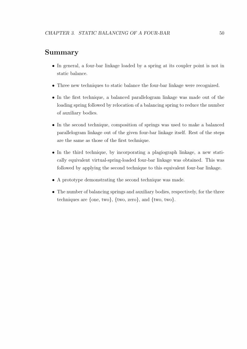
CHAPTER 3. STATIC BALANCING OF A FOUR-BAR 50
Summary
• In general, a four-bar linkage loaded by a spring at its coupler point is not in
static balance.
• Three new techniques to static balance the four-bar linkage were recognized.
• In the first technique, a balanced parallelogram linkage was made out of the
loading spring followed by relocation of a balancing spring to reduce the number
of auxiliary bodies.
• In the second technique, composition of springs was used to make a balanced
parallelogram linkage out of the given four-bar linkage itself. Rest of the steps
are the same as those of the first technique.
• In the third technique, by incorporating a plagiograph linkage, a new stati-
cally equivalent virtual-spring-loaded four-bar linkage was obtained. This was
followed by applying the second technique to this equivalent four-bar linkage.
• A prototype demonstrating the second technique was made.
• The number of balancing springs and auxiliary bodies, respectively, for the three
techniques are {one, two}, {two, zero}, and {two, two}.
Chapter 4
Static balance of the cognates of a
four-bar linkage
Overview
• Cognates of a four-bar linkage and its properties
• Quest for a unified parameterization of static balancing variables for the three
cognates.
• A geometric problem and its solution leading to a unified parameterization that
may be considered as an extension of Roberts-Chebyshev cognate theorem.
4.1 Introduction
4.1.1 Cognates
In kinematics of rigid-body linkages, it is well known that for a given four-bar linkage
and a coupler point on it, one can find two more four-bar linkages and corresponding
coupler points such that the coupler curves of all the three four-bar linkages are
the same. The three four-bar linkages are called cognates of each other. Figure
(4.1) shows a set of three cognates: B1C1D1B2, B2C2D2B3 and B3C3D3B1. In the
51

CHAPTER 4. STATIC BALANCE OF THE COGNATES 52
configuration shown in the figure, the coupler points are coincident at E. The triangle
formed by the ground anchor points, △B1B2B3, is called the cognate triangle. There
are a few interesting properties involving this triangle, as could be seen in [10]. One
such property is that △C1D1E, △EC2D2, and △D3EC3 are similar to the cognate
triangle B1B2B3. The cognates and their properties are summarized in what is called
Roberts-Chebyshev Cognate theorem (see [10]).
B3
γ2
γ1
γ2
γ3 γ1
γ2
γ3
γ1
D1
B2
D2
C2
C3
γ3
D3
C1
B1
E
kl
K
Figure 4.1: The cognates of a four-bar mechanism taking a load spring along theircommon coupler curve
4.1.2 Static balancing parameters and the cognates
A designer seeking to statically balance a given spring-loaded four-bar linkage has to
evaluate a family of feasible balancing parameters for each of the options under the
three techniques (see table 3.1) before choosing the one that best meets the design
requirements, including practical considerations. A more general design problem

CHAPTER 4. STATIC BALANCE OF THE COGNATES 53
would be to design a four-bar linkage that would guide the load spring along a specified
path and then statically balance the linkage so that the load spring can be moved
along the path effortlessly. If a four-bar linkage with its coupler curve matching the
specified path is found, then by Roberts-Chebyshev cognate theorem, it follows that
there are two more four-bar linkages whose coupler curves also match the specified
path. In order to make the best design choice, the designer has to evaluate feasible
balancing parameters of options under techniques 2 and 3, described in Chapter 3,
on all the three cognates. This chapter presents a result that will aid the designer to
evaluate these feasible balancing parameters on all the cognates in a unified manner.
As far as technique 1 is concerned, balancing parameters can be evaluated independent
of the four-bar linkage.
Since three four-bar linkages are considered in this chapter, balancing parameters
of techniques 2 and 3, such as H, kb, kt, W , U , and L, are subscripted with 1, 2, or
3, to correspond to the first, the second or the third cognate. Since all the cognates
are evaluated for the same load spring, K and kl are the same for all the cognates.
Among the balancing parameters, it is sufficient to focus only on Hi, kbi , and kti ,
i = 1, 2, or 3, since the remaining parameters are not variables. Nevertheless, to
determine the locus of Hi and the relation between Hi, kbi and kti (see equations (3.1
– 3.3) and equations (3.4 – 3.7)), it is necessary to know the remaining parameters.
While the remaining parameters can be deduced from the details of loaded ith cognate
linkage, table 4.1 shows that the detail is not necessary if the cognate triangle and
the ground anchor point of the loading spring are known.
Figure (4.2) shows the anchor point of a loading spring and a cognate triangle
where each side corresponds to a cognate. Sides corresponding to cognates 1, 2 and
3 are labelled as s1, s2 and s3, respectively. When an option of technique 2 or 3 is
applied on all the cognates with the cyclic symmetry, the straight-line loci of H1, H2
and H3, which are labelled as l1, l2 and l3, could be drawn, as illustrated in figures
(4.3), (4.4) and (4.5). Note that for both techniques, the origin for l1, l2 and l3 is one
of the vertices of the cognate triangle and there is one-one and onto relation between
the origins and the vertices. Because of this feature, it is now shown that H1, H2
and H3, can be varied as if they are at the vertices of the cognate triangle that is

CHAPTER 4. STATIC BALANCE OF THE COGNATES 54
Table 4.1: Deduction of various quantities in equations (3.1 – 3.7) from the cognatetriangle
Quantities other than H, kb and kt in equations (3.1 – 3.7):K, U , W , m, α, L
K Anchor point of the loading springW Base pivot of the balanced parallelogram
⇒ Coincident with a fixed pivot of the four-bar linkage⇒ One of the vertices of the cognate triangle∵ fixed pivots of cognates form the cognate triangle (see figure (4.1))
U Base pivot of the plagiograph⇒ One of the vertices of the cognate triangle (for the same reasons as of W )
m Ratio of two sides of the coupler triangle (see figures (3.9a) and (3.10))⇒ Ratio of two sides of the cognate triangle∵ the cognate triangle is similar to the coupler triangle (see figure (4.1))
α An angle of the coupler triangle (see figures (3.9a) and (3.10))⇒ An angle of the cognate triangle (∵ cognate △ ∼ coupler △)
L Anchor point of the equivalent of the loading spring (see figure (3.9b))
Found using the equation−→UL = mRα(
−−→UK). (U , m, α and K are as above.)
undergoing scaling and rotation transformation about a fixed point, while remaining
at the same time on their respective loci l1, l2 and l3. When H1, H2 and H3 are
varied as noted above, kb1 , kb2 and kb3 also vary, but it would be shown that their
ratio remains constant. This result follows from a solution that we give in this chapter
to a problem in geometry. The way we formulate the problem and find its solution
are described next.
4.2 A geometric problem and its solution
Given a triangle and three straight lines originating from its three vertices, find three
points on the three lines so that they from a triangle that is similar to the given
triangle. With respect to figure (4.6), the problem may be stated as: find points
Sa, Sb and Sc on straight lines a, b and c respectively, so that △SaSbSc is similar to
△ABC.

CHAPTER 4. STATIC BALANCE OF THE COGNATES 55
K
Cognate triangle
Common anchor point of load springs
B3
s2
s3
s1
B2B1
Figure 4.2: A cognate triangle and the ground anchor point of a load spring
K
U1, W1 : B2
U2, W2 : B3
U3, W3 : B1
B2, W1, U1s1
s2
s3
L1
L2
L3
B3, W2, U2l1
l2
l3
B1, W3, U3
Figure 4.3: Technique 3: the base pivot of the plagiograph (U) and the base of thebalanced parallelogram (W) for every cognate are not coincident.

CHAPTER 4. STATIC BALANCE OF THE COGNATES 56
K
U1 : B2 ; W1 : B1U2 : B3 ; W2 : B2U3 : B1 ; W3 : B3
B1
s2
s3
L1
L2
L3
s1
B3
B2
l1
l2
l3
Figure 4.4: Technique 3: the base pivot of the plagiograph (U) and the base of thebalanced parallelogram (W) for every cognate are coincident.

CHAPTER 4. STATIC BALANCE OF THE COGNATES 57
K
W1 : B2
W2 : B3
W3 : B1
B2, W1s1
s2
s3
l1
l2
l3
B1, W3
B3, W2
Figure 4.5: Technique 2: the base of the balanced parallelogram (W) at the indicatedvertices of the cognate triangle.

CHAPTER 4. STATIC BALANCE OF THE COGNATES 58
Ba
c
A
C
b
Figure 4.6: A problem in planar geometry
The method to obtain Sa, Sb and Sc varies for the following three cases, as de-
scribed next.
4.2.1 Case (i): a, b and c are parallel.
Sa, Sb and Sc can be obtained by translating A, B and C along the parallel lines, as
shown in figure (4.7), so that Sa, Sb and Sc stay on lines a, b and c while △SaSbSc is
congruent to △ABC.
b
AC
B
c
a
Sa
Sb
Sc
Figure 4.7: Finding Sa, Sb, and Sc in case(i)
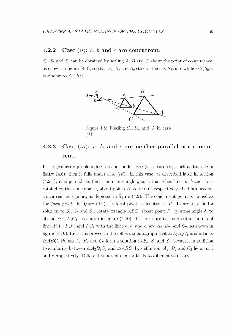
CHAPTER 4. STATIC BALANCE OF THE COGNATES 59
4.2.2 Case (ii): a, b and c are concurrent.
Sa, Sb and Sc can be obtained by scaling A, B and C about the point of concurrence,
as shown in figure (4.8), so that Sa, Sb and Sc stay on lines a, b and c while △SaSbSc
is similar to △ABC.
b
A
C
Bca Sb
Sa
Sc
Figure 4.8: Finding Sa, Sb, and Sc in case(ii)
4.2.3 Case (iii): a, b, and c are neither parallel nor concur-
rent.
If the geometric problem does not fall under case (i) or case (ii), such as the one in
figure (4.6), then it falls under case (iii). In this case, as described later in section
(4.2.4), it is possible to find a non-zero angle η such that when lines a, b and c are
rotated by the same angle η about points A, B, and C, respectively, the lines become
concurrent at a point, as depicted in figure (4.9). The concurrent point is named as
the focal pivot. In figure (4.9) the focal pivot is denoted as P . In order to find a
solution to Sa, Sb and Sc, rotate triangle ABC, about point P , by some angle δ, to
obtain △A1B1C1, as shown in figure (4.10). If the respective intersection points of
lines PA1, PB1, and PC1 with the lines a, b, and c, are A2, B2, and C2, as shown in
figure (4.10), then it is proved in the following paragraph that △A2B2C2 is similar to
△ABC. Points A2, B2 and C2 form a solution to Sa, Sb and Sc, because, in addition
to similarity between △A2B2C2 and △ABC, by definition, A2, B2 and C2 lie on a, b
and c respectively. Different values of angle δ leads to different solutions.

CHAPTER 4. STATIC BALANCE OF THE COGNATES 60
b
AC
B
c
a
P
η
ηη
Figure 4.9: Description of focal pivot
b
AC
B
c
a
P
η
ηη
δ
δ
δ
A1B1
C1
SaSb
Sc
Figure 4.10: Points A2, B2 and C2 form a solution to Sa, Sb and Sc
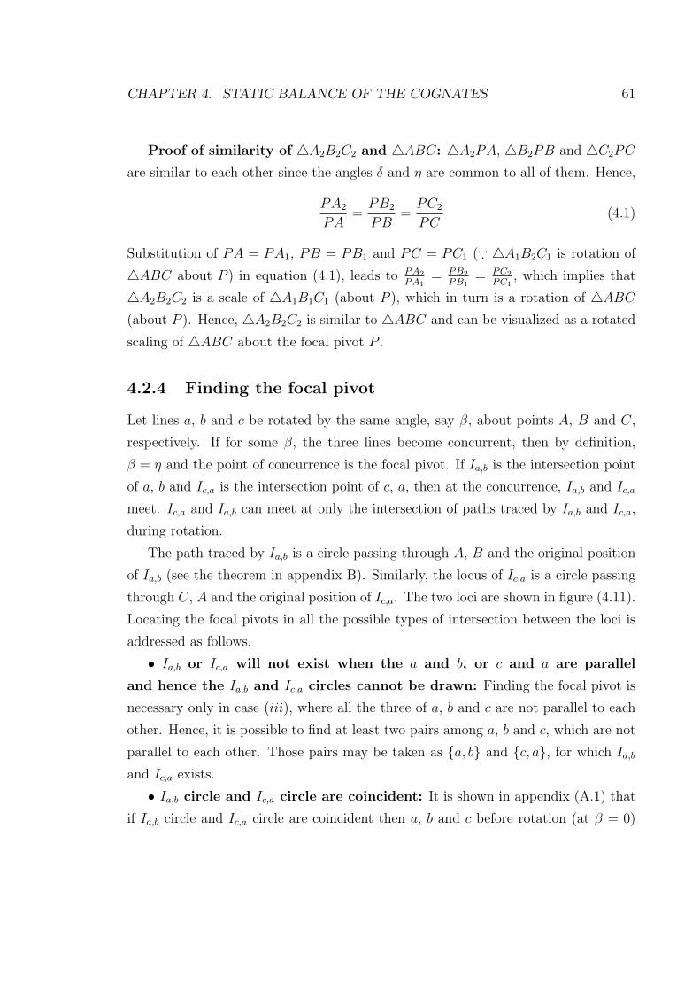
CHAPTER 4. STATIC BALANCE OF THE COGNATES 61
Proof of similarity of △A2B2C2 and △ABC: △A2PA, △B2PB and △C2PC
are similar to each other since the angles δ and η are common to all of them. Hence,
PA2
PA=PB2
PB=PC2
PC(4.1)
Substitution of PA = PA1, PB = PB1 and PC = PC1 (∵ △A1B2C1 is rotation of
△ABC about P ) in equation (4.1), leads to PA2
PA1= PB2
PB1= PC2
PC1, which implies that
△A2B2C2 is a scale of △A1B1C1 (about P ), which in turn is a rotation of △ABC
(about P ). Hence, △A2B2C2 is similar to △ABC and can be visualized as a rotated
scaling of △ABC about the focal pivot P .
4.2.4 Finding the focal pivot
Let lines a, b and c be rotated by the same angle, say β, about points A, B and C,
respectively. If for some β, the three lines become concurrent, then by definition,
β = η and the point of concurrence is the focal pivot. If Ia,b is the intersection point
of a, b and Ic,a is the intersection point of c, a, then at the concurrence, Ia,b and Ic,a
meet. Ic,a and Ia,b can meet at only the intersection of paths traced by Ia,b and Ic,a,
during rotation.
The path traced by Ia,b is a circle passing through A, B and the original position
of Ia,b (see the theorem in appendix B). Similarly, the locus of Ic,a is a circle passing
through C, A and the original position of Ic,a. The two loci are shown in figure (4.11).
Locating the focal pivots in all the possible types of intersection between the loci is
addressed as follows.
• Ia,b or Ic,a will not exist when the a and b, or c and a are parallel
and hence the Ia,b and Ic,a circles cannot be drawn: Finding the focal pivot is
necessary only in case (iii), where all the three of a, b and c are not parallel to each
other. Hence, it is possible to find at least two pairs among a, b and c, which are not
parallel to each other. Those pairs may be taken as {a, b} and {c, a}, for which Ia,b
and Ic,a exists.
• Ia,b circle and Ic,a circle are coincident: It is shown in appendix (A.1) that
if Ia,b circle and Ic,a circle are coincident then a, b and c before rotation (at β = 0)
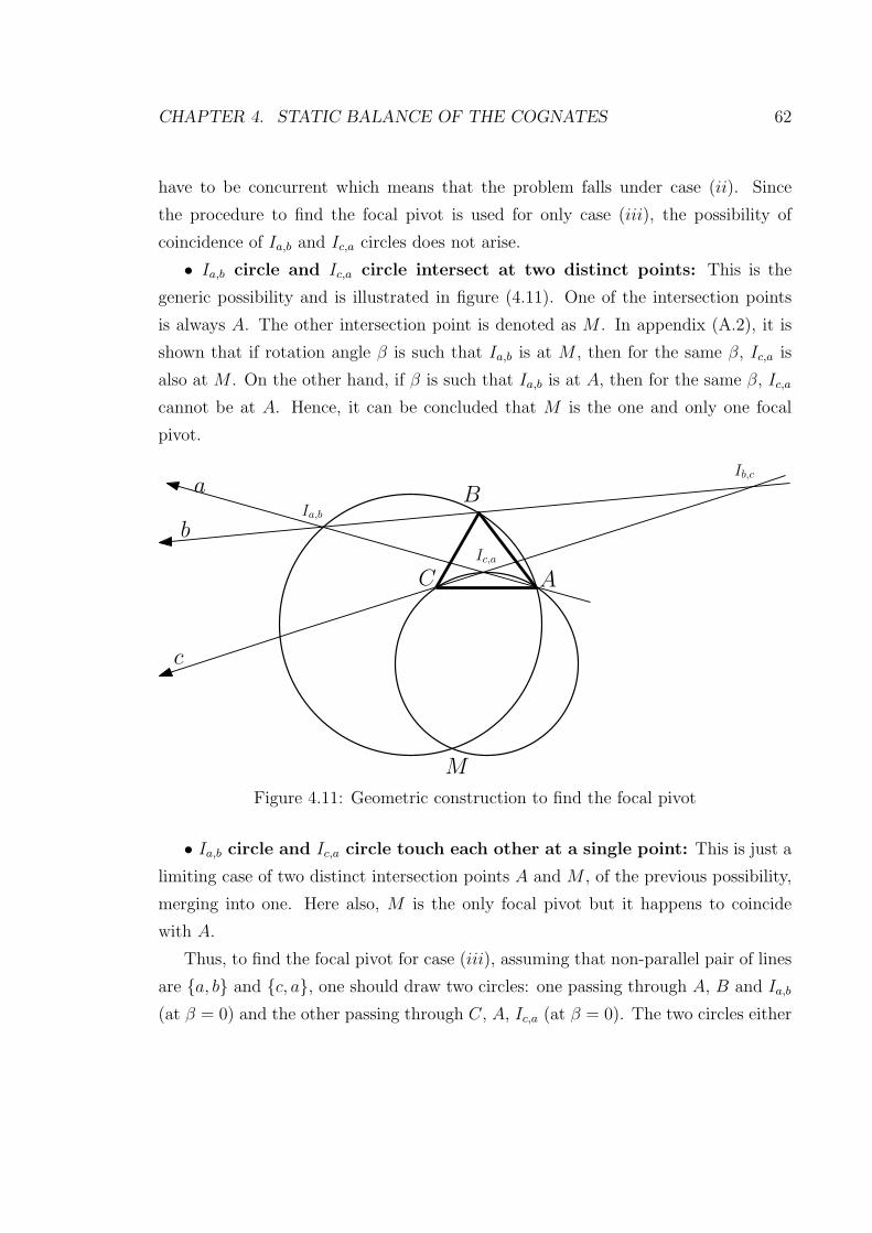
CHAPTER 4. STATIC BALANCE OF THE COGNATES 62
have to be concurrent which means that the problem falls under case (ii). Since
the procedure to find the focal pivot is used for only case (iii), the possibility of
coincidence of Ia,b and Ic,a circles does not arise.
• Ia,b circle and Ic,a circle intersect at two distinct points: This is the
generic possibility and is illustrated in figure (4.11). One of the intersection points
is always A. The other intersection point is denoted as M . In appendix (A.2), it is
shown that if rotation angle β is such that Ia,b is at M , then for the same β, Ic,a is
also at M . On the other hand, if β is such that Ia,b is at A, then for the same β, Ic,a
cannot be at A. Hence, it can be concluded that M is the one and only one focal
pivot.
Ia,b
AC
B
c
a
Ic,a
Ib,c
b
M
Figure 4.11: Geometric construction to find the focal pivot
• Ia,b circle and Ic,a circle touch each other at a single point: This is just a
limiting case of two distinct intersection points A and M , of the previous possibility,
merging into one. Here also, M is the only focal pivot but it happens to coincide
with A.
Thus, to find the focal pivot for case (iii), assuming that non-parallel pair of lines
are {a, b} and {c, a}, one should draw two circles: one passing through A, B and Ia,b
(at β = 0) and the other passing through C, A, Ic,a (at β = 0). The two circles either
CHAPTER 4. STATIC BALANCE OF THE COGNATES 63
intersect at two distinct points: M and A, or touch at the point A. In the former
case, the focal pivot is M and in the later case it is A.
4.3 The result
The common properties of solution to Sa, Sb and Sc in all the possible cases presented
in sections 4.2.1, 4.2.2 and 4.2.3, are summarized below.
• Property 1: The set of possibilities for Sa, Sb and Sc constitute a one-parameter
set. A convenient parameter parameterizing the set in case (i) is the translation,
in case (ii) is the scale factor, and in case (iii) is the rotation angle δ.
• Property 2: The ratio ASa : BSb : CSc is the same throughout the one-
parameter set, even though ASa, BSb and CSc themselves vary over the set. The
ratio is 1 : 1 : 1 in case (i), PA : PB : PC in case (ii), and again PA : PB : PC
in case (iii) (see equation (4.1) where A2, B2 and C2 are solutions to Sa, Sb and
Sc).
These properties are now applied to the cognate triangle and loci l1, l2, and l3, as
described next.
4.3.1 A parameterization of the balancing parameters of the
three cognates that has cognate triangle related invari-
ants
The solutions given in section (4.2) are now applied to the cognate triangle and loci
of H shown in figures (4.3–4.5), by taking A, B, C, a, b, c, Sa, Sb, Sc as W1, W2, W3
(the vertices of the cognate triangle), l1, l2, l3, H1, H2, H3, respectively. Then, the
properties at the end of section (4.2) take the following form:
There is a one-parameter parameterization of the balancing parameters of the three
cognates where
• △H1H2H3 is similar to △W1W2W3 (the cognate triangle), and
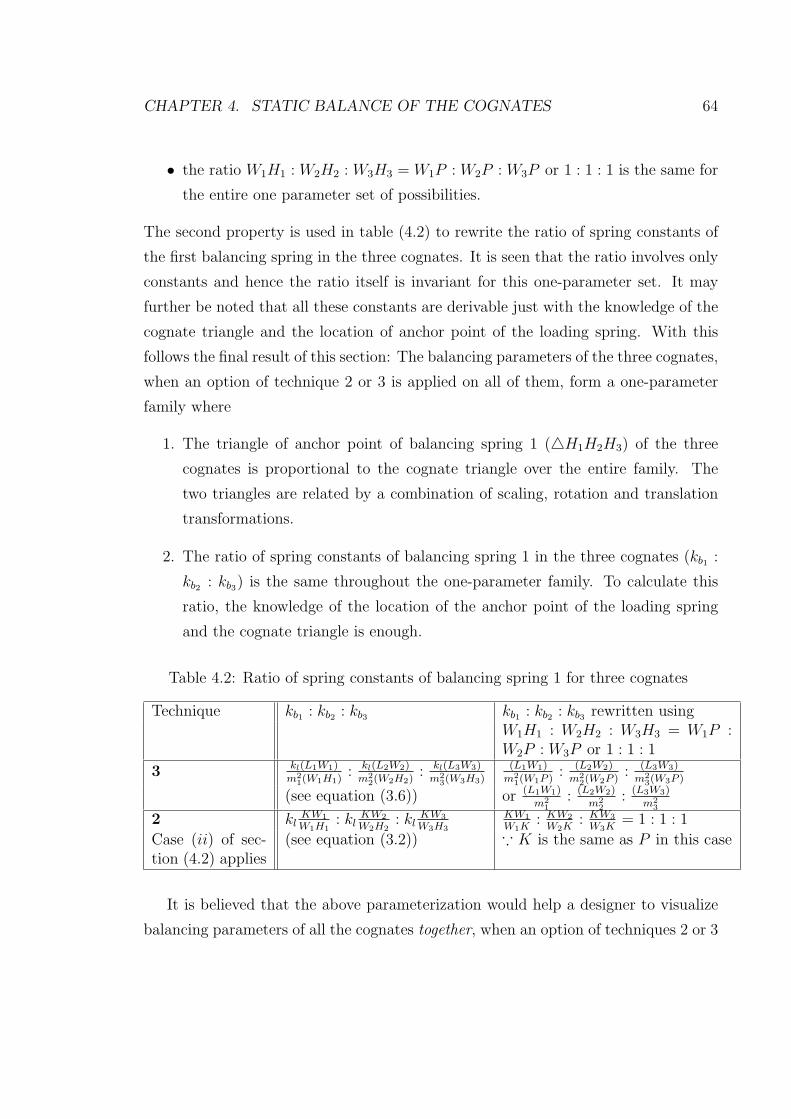
CHAPTER 4. STATIC BALANCE OF THE COGNATES 64
• the ratio W1H1 : W2H2 : W3H3 = W1P : W2P : W3P or 1 : 1 : 1 is the same for
the entire one parameter set of possibilities.
The second property is used in table (4.2) to rewrite the ratio of spring constants of
the first balancing spring in the three cognates. It is seen that the ratio involves only
constants and hence the ratio itself is invariant for this one-parameter set. It may
further be noted that all these constants are derivable just with the knowledge of the
cognate triangle and the location of anchor point of the loading spring. With this
follows the final result of this section: The balancing parameters of the three cognates,
when an option of technique 2 or 3 is applied on all of them, form a one-parameter
family where
1. The triangle of anchor point of balancing spring 1 (△H1H2H3) of the three
cognates is proportional to the cognate triangle over the entire family. The
two triangles are related by a combination of scaling, rotation and translation
transformations.
2. The ratio of spring constants of balancing spring 1 in the three cognates (kb1 :
kb2 : kb3) is the same throughout the one-parameter family. To calculate this
ratio, the knowledge of the location of the anchor point of the loading spring
and the cognate triangle is enough.
Table 4.2: Ratio of spring constants of balancing spring 1 for three cognates
Technique kb1 : kb2 : kb3 kb1 : kb2 : kb3 rewritten usingW1H1 : W2H2 : W3H3 = W1P :W2P : W3P or 1 : 1 : 1
3 kl(L1W1)
m21(W1H1)
: kl(L2W2)
m22(W2H2)
: kl(L3W3)
m23(W3H3)
(L1W1)
m21(W1P )
: (L2W2)
m22(W2P )
: (L3W3)
m23(W3P )
(see equation (3.6)) or (L1W1)
m21
: (L2W2)
m22
: (L3W3)
m23
2 klKW1
W1H1: kl
KW2
W2H2: kl
KW3
W3H3
KW1
W1K: KW2
W2K: KW3
W3K= 1 : 1 : 1
Case (ii) of sec-tion (4.2) applies
(see equation (3.2)) ∵ K is the same as P in this case
It is believed that the above parameterization would help a designer to visualize
balancing parameters of all the cognates together, when an option of techniques 2 or 3

CHAPTER 4. STATIC BALANCE OF THE COGNATES 65
is being evaluated. This result may be seen as an extension of the Roberts-Chebyshev
cognate theorem to static balancing.
Summary
• Cognates of a four-bar linkage have the same coupler curve.
• When static balancing parameters of the three cognates are considered together,
one can have a unified parameterization with properties related to the cognate
triangle.
• As the unified parameter varies, the triangle formed by the anchor points of the
balancing springs remain similar to the cognate triangle.
• Under the unified parameterization, the ratio of spring constants of a set of
corresponding balancing springs is constant.
• The constant ratio can be geometrically determined from the knowledge of the
cognate triangle and the anchor point of the balancing spring.
• In summary, the results of this chapter may be considered as an extension of
the classical theorem on cognates to static balancing.

Chapter 5
Static balancing of planar linkages
without auxiliary bodies
Overview
• Statically balancing a lever under spring loads and gravity loads.
• Statically balancing the rotational motion of a rigid-body that is free to move
in a plane by addition of springs.
• Transforming potential energy dependence from one body to another body
through a common point of the bodies.
• Recursive application of the transformation to statically balance any revolute-
jointed linkage that is under gravity and or spring loads.
• Examples demonstrating the recursive method.
5.1 Introduction
Figure (5.1a) shows a 4R linkage under a gravity load on its last link. This load
is balanced by counterweights added all through the linkage. Note the pattern of
weights; infact this balancing method extends to a general n-body revolute-jointed
66
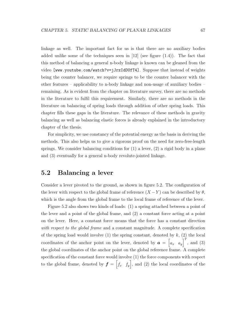
CHAPTER 5. STATIC BALANCING OF PLANAR LINKAGES 67
linkage as well. The important fact for us is that there are no auxiliary bodies
added unlike some of the techniques seen in [12] (see figure (1.4)). The fact that
this method of balancing a general n-body linkage is known can be gleaned from the
video [www.youtube.com/watch?v=jJrzIdDUfT4]. Suppose that instead of weights
being the counter balancer, we require springs to be the counter balancer with the
other features – applicability to n-body linkage and non-usage of auxiliary bodies –
remaining. As is evident from the chapter on literature survey, there are no methods
in the literature to fulfil this requirement. Similarly, there are no methods in the
literature on balancing of spring loads through addition of other spring loads. This
chapter fills these gaps in the literature. The relevance of these methods in gravity
balancing as well as balancing elastic forces is already explained in the introductory
chapter of the thesis.
For simplicity, we use constancy of the potential energy as the basis in deriving the
methods. This also helps us to give a rigorous proof on the need for zero-free-length
springs. We consider balancing conditions for (1) a lever, (2) a rigid body in a plane
and (3) eventually for a general n-body revolute-jointed linkage.
5.2 Balancing a lever
Consider a lever pivoted to the ground, as shown in figure 5.2. The configuration of
the lever with respect to the global frame of reference (X−Y ) can be described by θ,
which is the angle from the global frame to the local frame of reference of the lever.
Figure 5.2 also shows two kinds of loads: (1) a spring attached between a point of
the lever and a point of the global frame, and (2) a constant force acting at a point
on the lever. Here, a constant force means that the force has a constant direction
with respect to the global frame and a constant magnitude. A complete specification
of the spring load would involve (1) the spring constant, denoted by k, (2) the local
coordinates of the anchor point on the lever, denoted by a =[
ax ay
]T
, and (3)
the global coordinates of the anchor point on the global reference frame. A complete
specification of the constant force would involve (1) the force components with respect
to the global frame, denoted by f =[
fx fy
]
, and (2) the local coordinates of the

CHAPTER 5. STATIC BALANCING OF PLANAR LINKAGES 68
Balancing loads :Springs
Balancing loads :Springs
? ?
(a) (b) (c)
Original load
Original load(black colored)balanced bycounterweights(grey colored)
Original load
Original load
Figure 5.1: Lack of methods for spring-based n-body linkage balancing without theusage of auxiliary bodies
point of action of the force on the lever, denoted by p =[
px py
]
.
5.2.1 Potential energy as a function of the configuration vari-
able
By referring to figure (5.2), the potential energy of the constant load is
PEc = −fT (r +R (θ)p) (5.1)

CHAPTER 5. STATIC BALANCING OF PLANAR LINKAGES 69
θ
xy
Xa
k
b
p
f
X
Y r
d
Figure 5.2: A lever under a constant load and a spring load
where r =[
rx ry
]T
is the coordinates of the origin of the local frame on the lever
with respect to the global frame and R is the rotation matrix function given by
R (ψ) =
[
cosψ − sinψ
sinψ cosψ
]
for any angle ψ (5.2)
The potential energy of the spring is
PEs =k
2(l − l0)
2 =k
2l2 − kl0l +
k
2l20 (5.3)
where l0 is the free length of the spring and l is the magnitude of d, the displacement of
one-end point of the spring with respect to the other. This d, referring to figure (5.2),
is:
d = (r +R (θ)a)− b (5.4)
Since l2 = dTd, the potential energy in expression (5.3) may be rewritten as
PEs =k
2dTd− kl0
√
dTd+k
2l20 (5.5)

CHAPTER 5. STATIC BALANCING OF PLANAR LINKAGES 70
If the free-length of the spring is zero, then only the first term in equation (5.5)
remains and hence we call it as PEs,zero, i.e.,
PEs,zero =k
2dTd =
k
2((r +R (θ)a)− b)T ((r +R (θ)a)− b)
=k
2(rTr + aTRT (θ)R(θ)a+ bTb− 2rTb+ 2rTR(θ)a
− 2bTR(θ)a)
=k
2
(rTr + aTa+ bTb− 2rTb+ 2rTR(θ)a− 2bTR(θ)a
)(5.6)
∵ RT (θ)R(θ) = I
Since the remaining last two terms of the potential energy in equation (5.5) are non-
zero only if free-length l0 is non-zero, we name these terms as PEs,nonzero, i.e.,
PEs,nonzero = −kl0√
dTd+k
2l20 (5.7)
From equation (5.6), it follows that dTd = 2kPEs,zero. Substituting this in equation
(5.7) leads to the following expression for PEs,nonzero.
PEs,nonzero = −l0√
2kPEs,zero +k
2l20 (5.8)
In the expressions of the potential energy in equations (5.1), (5.6) and (5.8), as
the configuration of the lever varies, f , p, a, b, k, l0 remain constants and r is made
a constant by choosing the origin of the local frame on the lever to coincide with
the pivot point. The dependency of the expressions on the configuration is due the
matrix R(θ), which by examining the definition of R in equation (5.2), can be split
as:
R(θ) =
[
1 0
0 1
]
cos θ +
[
0 −1
1 0
]
sin θ = I cos θ +R(π
2) sin θ (5.9)
This form of R(θ) indicates that PEc in equation (5.1) and PEs,zero in equation
(5.6) can be written as a linear combination of sin θ, cos θ, and 1 (for constants).
The coefficients of sin θ, cos θ and 1 are presented, for clarity, in a tabular form in

CHAPTER 5. STATIC BALANCING OF PLANAR LINKAGES 71
Table 5.1: Potential energy of the weight and the zero-free-length component of thespring acting on the lever is a linear combination of cos θ, sin θ, and 1.
Basis CoefficientsWeight Zero-free-length component of spring load
cos θ −fTp
= − (fypy + fxpx)k (r − b)T a
= k (ayry + axrx − ayby − axbx)
sin θ −fTR(π2) p
= (fxpy − fypx)k (r − b)T R(π
2) a
= k(axry − ayrx − axby + aybx)
1 −fTr
= −fyry − fxrx
+ki2
(rTr + aTa+ bTb− 2rTb
)
= +ki2(r2y−2byry+r
2x−2bxrx+b
2y+b
2x+a
2y+a
2x)
table 5.1. Thus, we now have potential energy of constant and spring loads expressed
as functions of configuration variable θ.
5.2.2 Invariance of potential energy with respect to the con-
figuration variable
Trivial conditions
The potential energy of the spring on the lever can have constant potential energy
only under trivial conditions: (1) the spring stiffness is zero (k = 0), (2) the anchor
point on the lever is at the hinge point (a = 0), and (3) the anchor point on the global
frame is at the hinge point (b = r). Similar trivial conditions for the constant loads
are: (1) the load is zero (f = 0), and (2) the load acts at the pivot point (p = 0).
It is only under these trivial conditions that the coefficients of cos θ and sin θ become
zero in table 5.1.
The discovery of Lucien LaCoste
Even though a non-trivial spring and a non-trivial constant load cannot be individu-
ally in static balance, they together can be so, as demonstrated in figure (5.3). This
was first recognized by Lucien LaCoste (see [3]) in the context of having a pendulum
of infinite period. Figure (5.3) shows a lever under the action of a weight W that is
balanced by a zero-free-length spring of spring constant k anchored above the pivot

CHAPTER 5. STATIC BALANCING OF PLANAR LINKAGES 72
of the lever at a height of h. As shown in the figure, under the condition W = kh,
the potential energy is invariant with respect to configuration variable θ.
X
xy
Y
θl
kh W
a = p =
[
l
0
]
b =
[
0h
]
f =
[
0−W
]
r =
[
00
]
zero-free-length spring
weight
PEc = (0) cos θ + (Wl) sin θ + constant
PEz = (0) cos θ + (−khl) sin θ + constant+
PEnet = (l (W − kh)) sin θ + constant
0
when W = kh
Figure 5.3: Static balancing of a weight by a spring
Several zero-free-length springs and constant loads
The balancing conditionW = kh of the example in figure (5.3) will now be generalized
to a lever under several constant loads and zero-free-length spring loads. Since several
loads are now being considered, let both constant loads and zero-free-length spring
loads be ordered to allow indexing. The notation ai, bi ki has the same meaning as
a, b and k in figure (5.2) other than that it corresponds to ith spring. f i and pi
also have similar meaning. Further, let the number of constant loads be nc and the
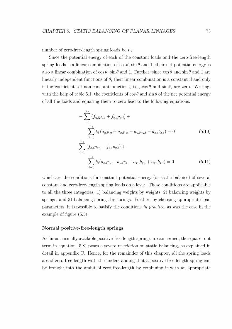
CHAPTER 5. STATIC BALANCING OF PLANAR LINKAGES 73
number of zero-free-length spring loads be ns.
Since the potential energy of each of the constant loads and the zero-free-length
spring loads is a linear combination of cos θ, sin θ and 1, their net potential energy is
also a linear combination of cos θ, sin θ and 1. Further, since cos θ and sin θ and 1 are
linearly independent functions of θ, their linear combination is a constant if and only
if the coefficients of non-constant functions, i.e., cos θ and sin θ, are zero. Writing,
with the help of table 5.1, the coefficients of cos θ and sin θ of the net potential energy
of all the loads and equating them to zero lead to the following equations:
−nc∑
i=1
(fy,ipy,i + fx,ipx,i)+
ns∑
i=1
ki (ay,iry + ax,irx − ay,iby,i − ax,ibx,i) = 0 (5.10)
nc∑
i=1
(fx,ipy,i − fy,ipx,i)+
ns∑
i=1
ki(ax,iry − ay,irx − ax,iby,i + ay,ibx,i) = 0 (5.11)
which are the conditions for constant potential energy (or static balance) of several
constant and zero-free-length spring loads on a lever. These conditions are applicable
to all the three categories: 1) balancing weights by weights, 2) balancing weights by
springs, and 3) balancing springs by springs. Further, by choosing appropriate load
parameters, it is possible to satisfy the conditions in practice, as was the case in the
example of figure (5.3).
Normal positive-free-length springs
As far as normally available positive-free-length springs are concerned, the square root
term in equation (5.8) poses a severe restriction on static balancing, as explained in
detail in appendix C. Hence, for the remainder of this chapter, all the spring loads
are of zero free-length with the understanding that a positive-free-length spring can
be brought into the ambit of zero free-length by combining it with an appropriate

CHAPTER 5. STATIC BALANCING OF PLANAR LINKAGES 74
θ
xy
Xa1
a2
ai
ans
k1
k2
ki
kns
b1
b2
bns
bi
p1
f1
p2
f2
pnc
fnc
X
Yr
Figure 5.4: A body that is free to move in a plane
negative-free-length spring.
Our next aim is to derive a set of conditions for the static balance of a revolute-
jointed multi-body linkage loaded by constant loads and zero-free-length spring loads.
Before that, it is useful to consider the static balance of a single rigid body moving
freely in a plane.
5.3 Balancing of a rigid body in a plane
Consider the rigid body shown in figure (5.2). An appropriate set of configuration
variables for the body is {r, θ}. It may be noted that r in figure (5.4), in contrast to
figure (5.2), is an independent variable because the body is free to move in the plane.
The loads on the body are a set of zero-free-length spring loads and constant
loads, and both sets of loads are exerted by the global frame of reference as shown
in figure (5.4). The notation nc, ns, ai, bi, ki, f i, and pi has the same meaning as
in Section 5.2. The potential energy of the loads is also the same as in Section 5.2

CHAPTER 5. STATIC BALANCING OF PLANAR LINKAGES 75
Table 5.2: Potential energy of weight and spring acting on a link moving in a plane.
Basis Coefficients of the basisWeight Spring load Generalized po-
tential (see eqn.(5.15)
cos θ −(fypy +fxpx)
−k(ayby + axbx) (qywy + qxwx)
sin θ +(fxpy −fypx)
−k(axby − aybx) (qxwy − qywx)
rx cos θ 0 kax vxry cos θ 0 kay vyrx sin θ 0 −kay −vyry sin θ 0 kax vxr2x 0 k
2κ
r2y 0 k2
κ
rx −fx −kbx uxry −fy −kby uy1 0 +k
2(a2x + a2y + b2x +
b2y)c
except that rx and ry are now independent variables. In table 5.1 of Section 5.2, when
linearly independent functions of {r, θ} are pulled out as basis functions, table 5.2
is obtained. As is evident from table 5.2, the potential energy of the loads is now
a linear combination of the following basis functions: cos θ, sin θ, rx cos θ, ry cos θ,
rx sin θ, ry sin θ, r2x, r
2y, rx, ry, and 1.
The net potential energy of nc constant loads and ns spring loads is also a linear
combinations of the same basis functions. Furthermore, cos θ, sin θ, rx cos θ, ry cos θ,
rx sin θ, ry sin θ, r2x, r
2y, rx, ry, and 1 are linearly independent functions of {r, θ}.
Hence, from a reasoning similar to the one in Section 5.2, for the net potential en-
ergy to be independent of the configuration variables, the coefficients of all the basis
functions other than 1 have to be zero. However, it is not practical to make the
coefficients of all these functions as zeros because of the following reasons:
• There are only gravity loads: Gravity is the most important practically seen
instance of a constant load. When all the constant loads are gravity loads,

CHAPTER 5. STATIC BALANCING OF PLANAR LINKAGES 76
f i = migi, where mi is the mass and g is the acceleration due to gravity.
Further, the coefficient of rx and ry become
(
−gxng∑
i=1
mi
)
and
(
−gyng∑
i=1
mi
)
.
Since mi > 0, ∀i,ng∑
i=1
mi > 0. Also, since the acceleration due to gravity is
non-zero, both gx and gy cannot be zero. Hence, the coefficients of both rx and
ry cannot be zero.
• There are zero-free-length spring loads, possibly with gravity loads: In
this case the coefficients of both r2x and r2y arens∑
i=1
ki. Since the spring constants
of all the springs considered here are positive (ki > 0, ∀i),ns∑
i=1
ki cannot be zero.
Hence, the coefficients of r2x and r2y cannot be zero.
However, as shown in appendix D.1, there is no such practical difficulty in making
the coefficients of all θ-dependent functions, i.e., cos θ, sin θ, rx cos θ, ry cos θ, rx sin θ,
and ry sin θ, to be zeros. Setting θ-dependent terms to zero amounts to the following
set of independent constraints:
−
nc∑
i=1
((fy,ipy,i + fx,ipx,i))−
ns∑
i=1
(ki(ay,iby,i + ax,ibx,i)) = 0 (5.12)
+
nc∑
i=1
((fx,ipy,i − fy,ipx,i))−
ns∑
i=1
(ki(ax,iby,i − ay,ibx,i)) = 0 (5.13)
ns∑
i=1
(kiai) = 0 (5.14)
It is shown in Appendix D.1 that if these constraints are not satisfied by the loads,
then by adding not more than two zero-free-length springs, these constraints can be
satisfied. A numerical example to demonstrate the same is given in figure (5.5) with
the details of the loads in table 5.3.
Inspite of being able to make the potential energy of the loads on the link inde-
pendent of θ, the dependency on r still remains. In Section 5.4, we show that if the
body is joined to an appropriate linkage, then by adding extra loads to other parts
of the linkage, the r-dependent terms of the potential energy can be balanced out.
Before we proceed to Section 5.4, it may be noted that the potential energy of a
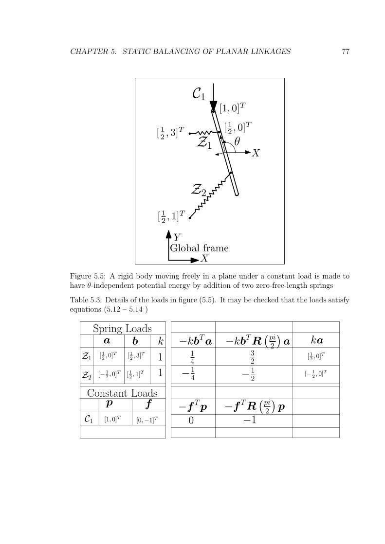
CHAPTER 5. STATIC BALANCING OF PLANAR LINKAGES 77
[ 12, 3]T
[ 12, 1]T
Global frameX
Y
[ 12, 0]T
[1, 0]T
Z1
Z2
C1
Xθ
Figure 5.5: A rigid body moving freely in a plane under a constant load is made tohave θ-independent potential energy by addition of two zero-free-length springs
Table 5.3: Details of the loads in figure (5.5). It may be checked that the loads satisfyequations (5.12 – 5.14 )
Spring Loadsa b k
Z1
Z2
[ 12, 0]T [ 1
2, 3]T 1
[− 1
2, 0]T [ 1
2, 1]T 1
Constant Loadsp f
C1 [1, 0]T [0,−1]T
−kbTa −kbTR(
pi
2
)
a ka1
4
−1
4
−fTp
0
−fTR(
pi
2
)
p
3
2
−1
2
−1
[ 12, 0]T
[− 1
2, 0]T

CHAPTER 5. STATIC BALANCING OF PLANAR LINKAGES 78
constant load or a zero-free-length spring load fall under the following general form:
Φ = rTu+ κrTr + rTR (θ)v +wTR (θ) q + c (5.15)
where θ and r are the configuration variables of the rigid body on which the load
acts. In the case of constant loads, by comparing equation (5.1) with equation (5.15),
we have
u = −f , κ = 0, v = 0, w = −f , q = p, and c = 0 (5.16)
and in the case of zero-free-length spring loads, by comparing equation (5.6) and
(5.15), we have
u = −kb, κ =k
2, v = ka, w = −b, q = ka, and c =
k
2
(bTb+ aTa
)
(5.17)
Later in the chapter, we encounter potential energy functions that are of the form
given in equation (5.15), but they cannot be attributed to zero-free-length spring loads
or constant loads acting on the body. Hence, there is a need to generalize constraints
(5.10), (5.11), (5.12), (5.13), and (5.14) to the form given in equation (5.15). Such
a generalization is possible because, as can be seen in the last column of table 5.2,
the potential given in equation (5.15) is a linear combination of the basis functions
given in table 5.2 just as in the case of constant and zero-free-length spring loads.
The following proposition states the generalization.
Proposition 1. If there are n functions of the form
Φi = rTui + κirTr + rTR (θ)vi +wTR (θ) qi + ci, i = 1 · · ·n (5.18)
with r and θ as the variables, thenn∑
i=1
Φi is independent of θ if and only if the following

CHAPTER 5. STATIC BALANCING OF PLANAR LINKAGES 79
constraints are satisfied:
n∑
i=1
(qy,iwy,i + qx,iwx,i) = 0 (5.19)
n∑
i=1
(qx,iwy,i − qy,iwx,i) = 0 (5.20)
n∑
i=1
vi = 0 (5.21)
When these constraints are satisfied,n∑
i=1
Φi depends only on r in the following form
n∑
i=1
Φi =n∑
i=1
(rTui + κir
Tr + ci)
=(rT)
n∑
i=1
ui +(rTr
)n∑
i=1
κi +n∑
i=1
ci (5.22)
Furthermore, if r happens to be a constant (as in a lever) with only θ being the
variable, thenn∑
i=1
Φi is independent of θ (and hence a constant) if and only if the
following constraints are satisfied:
n∑
i=1
(vy,iry + vx,irx + qy,iwy,i + qx,iwx,i) = 0 (5.23)
n∑
i=1
(vx,iry − vy,irx + qx,iwy,i − qy,iwx,i) = 0 (5.24)
Proof. The proof is along the same lines as the derivation of equations (5.10), (5.11),
(5.12), (5.13), and (5.14).
It may be noted that inspite of considering a general form of potential in equa-
tion (5.18), the inability to make the net potential energy independent of r remains
because of the following reason. In all the cases that we consider next, κi ≥ 0 and
κi > 0 for atleast one value of i. Hence, the r-dependent term,n∑
i=1
κirTr, cannot be
zero in the expression forn∑
i=1
Φi.

CHAPTER 5. STATIC BALANCING OF PLANAR LINKAGES 80
5.4 New static balancing techniques for revolute-
jointed linkages
If there is a single rigid body with loads exerted by a reference frame, then the net
potential energy of the loads depends on the configuration of the body with respect
to the reference frame. If there are several such bodies, then the net potential energy
of all the loads on all the bodies depends on the configuration of all the bodies. This
dependency on the configuration of all the bodies can be reduced to that of a single
body provided the bodies are connected by revolute joints (to begin with, say, in a
serial or a tree-structured manner) and the loads are zero-free-length spring loads and
constant loads. If this single body is the reference frame itself, then the net potential
energy is a constant (implying static balance) since the configuration of the reference
frame with respect to itself is always fixed. This result follows as a consequence of
the proposition that is presented next.
5.4.1 The potential energy of loads on a body transformed
as a function of another body
We are now considering several rigid bodies, each of them with its own r, θ, nc, ns,
ai, bi, ki, pi, etc. To distinguish these quantities belonging to different rigid bodies,
we number the rigid bodies and put the number as a superscript to these symbols.
Hence r, θ, nc, ns, ai, bi, ki, pi, and f i of body j are now represented as rj, θj, njc,
njs, a
ji , b
ji , k
ji , pi
j, etc.
Proposition 2. The net sum of a set of functions of the configuration variables of a
body l in the form given in equation (5.15), i.e.,
Φli = rlTul
i + κlirlTrl + rlTR
(θl)vli + wlTR
(θl)qli + cli, i = 1 · · ·nl (5.25)

CHAPTER 5. STATIC BALANCING OF PLANAR LINKAGES 81
can be expressed as a function of the same form but of body j, i.e.,
nl∑
i=1
Φli = Φj
i = rjTuji + κjir
jTrj + rjTR(
θj)
vji + wjTR
(
θj)
qji + cji (5.26)
provided the following conditions are satisfied:
• Condition 1: There is a point that is rigidly fixed to both body l and body j.
Such a point is called as a common point of bodies l and j.
• Condition 2: The origin of the local coordinate frame of body l is at the common
point.
• Condition 3: The sum of the set of functions of body l is dependent only on r
in the form given in equation (5.22).
Proof. Let the local coordinates of the common point required by condition 1 in body
l be slj and in body j be sjl . The commonality of the point can be written as follows.
rl +R(θl)slj = rj +R
(
θj)
sjl (5.27)
Condition 2 implies that slj = 0. Substituting slj = 0 into equation (5.27) leads to
rl = rj +R(
θj)
sjl (5.28)
Condition 3 implies that the sum of the set of functions of body l can be written as
nl∑
i=1
Φli = rlT
nl∑
i=1
uli +(
rlTrl
) nl∑
i=1
κli (5.29)
The constant term is omitted in equation (5.29) since it is inconsequential for the
discussion.
Substitution of rl from equation (5.28) into equation (5.29) and simplification
CHAPTER 5. STATIC BALANCING OF PLANAR LINKAGES 82
using the fact that RT (θ)R(θ) is identity lead to the following expression fornl∑
i=1
Φli:
rjT
uji
︷ ︸︸ ︷
nl∑
i=1
uli
+ rjTrj
κji
︷ ︸︸ ︷
nl∑
i=1
κli
+ rjTR(
θj)
vji
︷ ︸︸ ︷
2sjl
nl∑
i=1
κli
+
wji
T
︷ ︸︸ ︷
nl∑
i=1
uli
T
R(
θj)
qji
︷ ︸︸ ︷(
sjl
)
=nl∑
i=1
Φli = Φj
i (5.30)
Again, the constant term is omitted in equation (5.30). It may be readily recognized
that the sum of the set of functions on body l,nl∑
i=1
Φli, as seen in equation (5.30) is
indeed of the form given in equation (5.26).
5.4.2 Proposition 2 as the recursive relation of an iterative
static balancing algorithm
We now show that proposition 2 can be treated as a recursive relation that can be
incorporated into an iterative procedure to achieve static balance of a linkage. For the
purpose of this subsection, we restrict the linkage on which the iterative procedure
can be applied to have the following features:
1. The linkage should be tree-structured (i.e., no closed loops). This feature is
necessary since a recursive relation requires a tree-structure to propagate.
2. All the joints of the tree structure should be revolute joints. This feature is
necessary to satisfy condition 1 of proposition 2.
3. We want all the loads to have potential energy functions of the form given in
equation (5.25) of proposition 2. While we know that zero-free-length springs
and constant loads do have this form (see equations (5.16) and (5.17)) the fact

CHAPTER 5. STATIC BALANCING OF PLANAR LINKAGES 83
that there are several bodies involved requires a little attention. The configu-
ration variables(rl, θl
)of different bodies (i.e., of different l) should be with
respect to a common global frame of reference. Hence, constant loads on all
the bodies should be constant with respect to a common global reference frame
and any zero-free-length spring should have its one anchor point on the same
common global frame while the other anchor point can be on any of the bodies
constituting the linkage.
4. The common reference frame should be one of the bodies of the linkage, i.e., it
should join to body/bodies of the linkage by revolute joint/joints.
The iterative static balancing algorithm
We now present the iterative algorithm and prove that it leads to static balance.
Preparatory steps
1. Assign the reference body as the root node of the tree-structure (bodies are rep-
resented as nodes and joints as lines joining the nodes). With this assignment,
for every link/body other than the root, there is a parent body. Further, every
links other than the terminal links has one or more children.
2. On every link, choose a local frame that coincides with the center of the revolute
joint between the link and its parent. For every link k, rk and θk decide the
configuration of its local frame with respect to the frame of the root.
3. Give this tree-structure with the given constant and zero-free-length spring loads
(together referred to as original loads) as an input to the following iterative
procedure.
Iterative procedure
• Entry condition: If the tree-structure contains only the root node, then exit
from the iterative procedure. Otherwise, proceed to step 1.

CHAPTER 5. STATIC BALANCING OF PLANAR LINKAGES 84
• Step 1: Any terminal node l, has associated with it the following three kinds
of potential energy functions: 1) due to original loads on body l, 2) due to
association that happened in step 3 of previous iterations, and 3) additional
loads on body l. Let the number of such functions be represented by nlo, n
lc, n
la,
respectively. The first two kinds of functions are known from the given problem
and previous iterations, respectively, and the task in this step is to find the
additional loads so that
– case a: equations (5.19 - 5.21) are satisfied if l is not a child (i.e., not first
generation descendant) of the root.
– case b: equations (5.23 - 5.24) are satisfied if l is a child of the root. Note
that in this case rl is a constant because of the way local frame is chosen
in the preparatory steps.
This task makes sense only if the all kinds of potential energy functions fall
under the form of equation (5.15) with (r, θ) being(rl, θl
). The first and the
third kind of potential energy functions do fall under the form because of the
kind of loads we are considering (see equations (5.16) and (5.17)). The second
kind of potential energy functions conform to the form because of step 2, which
is in accordance with proposition 2. The critical role of proposition 2 in enabling
this iterative procedure may be noted. Further, Appendix D.2 asserts that the
task of this step is always feasible. It may be noted that there are several sets
of additional loads that satisfy these equations. This non-uniqueness calls for
discretion of the designer in choosing a suitable set of additional loads.
• Step 2: In case (a), expressnlo+nl
c+nla∑
i=1
Φli in the form given in equation (5.15)
where r and θ are the configuration variables of the parent of node l. This
is possible since condition 1 (because of revolute joint), condition 2 (because
of preparatory steps) and condition 3 (because of step 1) of proposition 2 are
satisfied. In case (b), recognize thatnlo+nl
c+nla∑
i=1
Φli is a constant as per proposition
1.
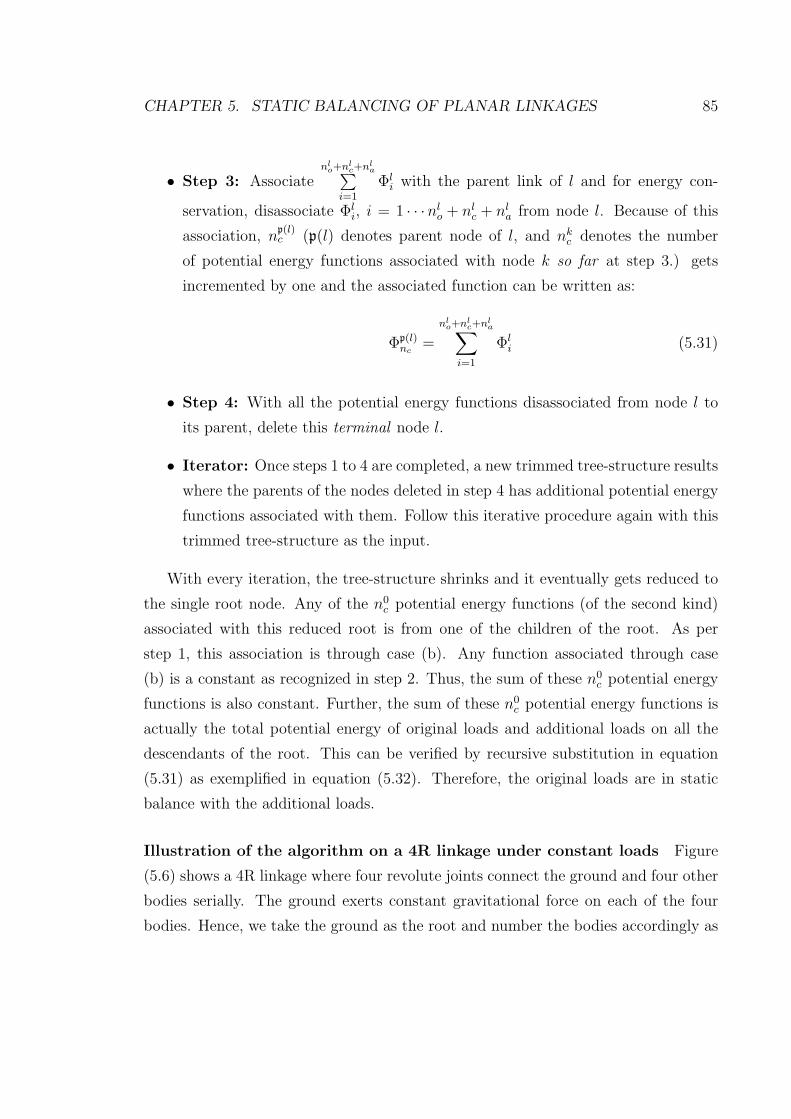
CHAPTER 5. STATIC BALANCING OF PLANAR LINKAGES 85
• Step 3: Associatenlo+nl
c+nla∑
i=1
Φli with the parent link of l and for energy con-
servation, disassociate Φli, i = 1 · · ·nl
o + nlc + nl
a from node l. Because of this
association, np(l)c (p(l) denotes parent node of l, and nk
c denotes the number
of potential energy functions associated with node k so far at step 3.) gets
incremented by one and the associated function can be written as:
Φp(l)nc
=
nlo+nl
c+nla∑
i=1
Φli (5.31)
• Step 4: With all the potential energy functions disassociated from node l to
its parent, delete this terminal node l.
• Iterator: Once steps 1 to 4 are completed, a new trimmed tree-structure results
where the parents of the nodes deleted in step 4 has additional potential energy
functions associated with them. Follow this iterative procedure again with this
trimmed tree-structure as the input.
With every iteration, the tree-structure shrinks and it eventually gets reduced to
the single root node. Any of the n0c potential energy functions (of the second kind)
associated with this reduced root is from one of the children of the root. As per
step 1, this association is through case (b). Any function associated through case
(b) is a constant as recognized in step 2. Thus, the sum of these n0c potential energy
functions is also constant. Further, the sum of these n0c potential energy functions is
actually the total potential energy of original loads and additional loads on all the
descendants of the root. This can be verified by recursive substitution in equation
(5.31) as exemplified in equation (5.32). Therefore, the original loads are in static
balance with the additional loads.
Illustration of the algorithm on a 4R linkage under constant loads Figure
(5.6) shows a 4R linkage where four revolute joints connect the ground and four other
bodies serially. The ground exerts constant gravitational force on each of the four
bodies. Hence, we take the ground as the root and number the bodies accordingly as
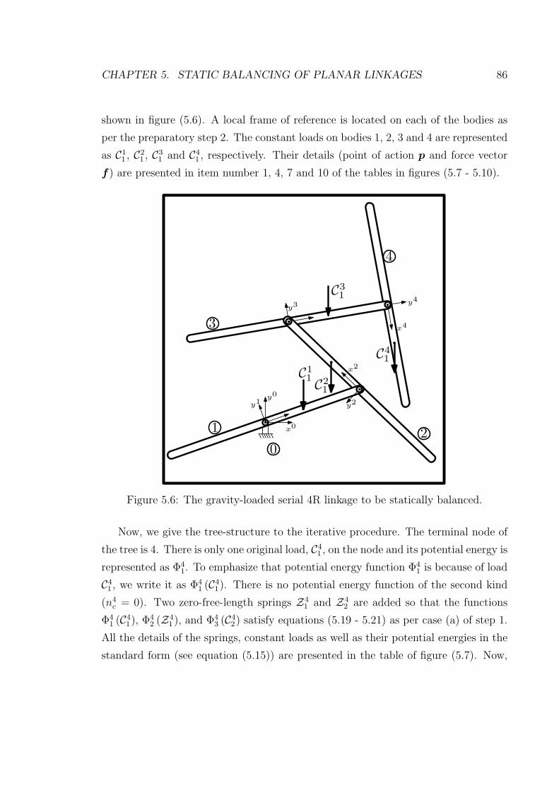
CHAPTER 5. STATIC BALANCING OF PLANAR LINKAGES 86
shown in figure (5.6). A local frame of reference is located on each of the bodies as
per the preparatory step 2. The constant loads on bodies 1, 2, 3 and 4 are represented
as C11 , C
21 , C
31 and C4
1 , respectively. Their details (point of action p and force vector
f) are presented in item number 1, 4, 7 and 10 of the tables in figures (5.7 - 5.10).
x0
y0
y1
1
y2
y3
x2
y4
x4
0
2
3
4
C1
1C2
1
C3
1
C4
1
Figure 5.6: The gravity-loaded serial 4R linkage to be statically balanced.
Now, we give the tree-structure to the iterative procedure. The terminal node of
the tree is 4. There is only one original load, C41 , on the node and its potential energy is
represented as Φ41. To emphasize that potential energy function Φ4
1 is because of load
C41 , we write it as Φ4
1 (C41). There is no potential energy function of the second kind
(n4c = 0). Two zero-free-length springs Z4
1 and Z42 are added so that the functions
Φ41 (C
41), Φ
42 (Z
41 ), and Φ4
3 (C42) satisfy equations (5.19 - 5.21) as per case (a) of step 1.
All the details of the springs, constant loads as well as their potential energies in the
standard form (see equation (5.15)) are presented in the table of figure (5.7). Now,
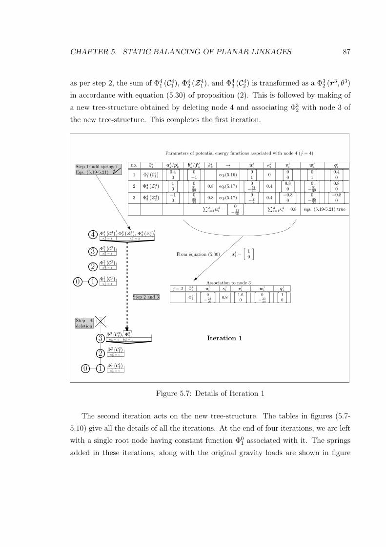
CHAPTER 5. STATIC BALANCING OF PLANAR LINKAGES 87
as per step 2, the sum of Φ41 (C
41), Φ
42 (Z
41 ), and Φ4
3 (C42) is transformed as a Φ3
2 (r3, θ3)
in accordance with equation (5.30) of proposition (2). This is followed by making of
a new tree-structure obtained by deleting node 4 and associating Φ32 with node 3 of
the new tree-structure. This completes the first iteration.
4
3
2
10
Φ4
1
(
C4
1
)
, Φ4
2
(
Z4
1
)
, Φ4
3
(
Z4
2
)
n4o
= 1 n4a
= 2
Φ3
1
(
C3
1
)
n3o
= 1
n2o
= 1
Φ2
1
(
C2
1
)
n1o
= 1
Φ1
1
(
C1
1
)
Step 1: add springs/Eqs. (5.19-5.21)
Iteration 13
2
10
n2o
= 1
Φ2
1
(
C2
1
)
n1o
= 1
Φ1
1
(
C1
1
)
Φ3
1
(
C3
1
)
, Φ3
2,
n3o
= 1 n3c
= 1
4
Step 2 and 3
Step 4:deletion
no. Φji a
jk/p
jk b
jk/f
jk k
jk → u
ji κ
ji v
ji w
ji q
ji
1 Φ4
1
(
C4
1
)
[
0.40
] [
0−1
]
eq.(5.16)
[
01
]
0
[
00
] [
01
] [
0.40
]
2 Φ4
2
(
Z4
1
)
[
10
] [
051
32
]
0.8 eq.(5.17)
[
0−
51
40
]
0.4
[
0.80
] [
0−
51
32
] [
0.80
]
3 Φ4
3
(
Z4
2
)
[
−10
] [
035
32
]
0.8 eq.(5.17)
[
0−
7
8
]
0.4
[
−0.80
] [
0−
35
32
] [
−0.80
]
∑
3
i=1u4
i =
[
0−
23
20
]
∑
3
i=1κ4
i = 0.8 eqs. (5.19-5.21) true
j = 3 Φj
i uj
i κj
i vj
i wj
i qj
i
Φ3
2
[
0
−
23
20
]
0.8
[
1.6
0
] [
0
−
23
20
] [
1
0
]
Parameters of potential energy functions associated with node 4 (j = 4)
s34=
[
10
]
From equation (5.30)
Association to node 3
Figure 5.7: Details of Iteration 1
The second iteration acts on the new tree-structure. The tables in figures (5.7-
5.10) give all the details of all the iterations. At the end of four iterations, we are left
with a single root node having constant function Φ01 associated with it. The springs
added in these iterations, along with the original gravity loads are shown in figure
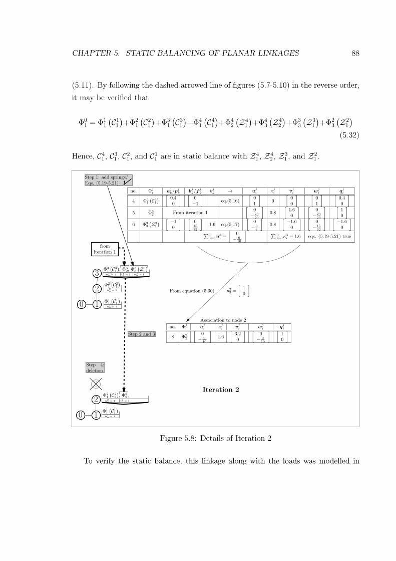
CHAPTER 5. STATIC BALANCING OF PLANAR LINKAGES 88
(5.11). By following the dashed arrowed line of figures (5.7-5.10) in the reverse order,
it may be verified that
Φ01 = Φ1
1
(C11
)+Φ2
1
(C21
)+Φ3
1
(C31
)+Φ4
1
(C41
)+Φ4
2
(Z4
1
)+Φ4
3
(Z4
2
)+Φ3
3
(Z3
1
)+Φ2
3
(Z2
1
)
(5.32)
Hence, C41 , C
31 , C
21 , and C1
1 are in static balance with Z41 , Z
42 , Z
31 , and Z2
1 .
3
2
10
n2o
= 1
Φ2
1
(
C2
1
)
n1o
= 1
Φ1
1
(
C1
1
)
Φ3
1
(
C3
1
)
, Φ3
2, Φ3
3
(
Z3
1
)
n3o
= 1 n3a
= 1n3c
= 1
fromiteration 1
Step 1: add springs/Eqs. (5.19-5.21)
2
10
n2o
= 1 n2c
= 1
Φ2
1
(
C2
1
)
, Φ2
2,
n1o
= 1
Φ1
1
(
C1
1
)
Step 2 and 3
Step 4:deletion
3
no. Φji a
jk/p
jk b
jk/f
jk k
jk → u
ji κ
ji v
ji w
ji q
ji
4 Φ3
1
(
C3
1
)
[
0.40
] [
0−1
]
eq.(5.16)
[
01
]
0
[
00
] [
01
] [
0.40
]
5 Φ3
2From iteration 1
[
0−
23
20
]
0.8
[
1.60
] [
0−
23
20
] [
10
]
6 Φ3
3
(
Z3
1
)
[
−10
] [
015
32
]
1.6 eq.(5.17)
[
0−
3
4
]
0.8
[
−1.60
] [
0−
15
32
] [
−1.60
]
∑
3
i=1u3
i =
[
0−
9
10
]
∑
3
i=1κ3
i = 1.6 eqs. (5.19-5.21) true
no. Φji u
ji κ
ji v
ji w
ji q
ji
8 Φ2
2
[
0−
9
10
]
1.6
[
3.20
] [
0−
9
10
] [
10
]
s23=
[
10
]
From equation (5.30)
Association to node 2
Iteration 2
Figure 5.8: Details of Iteration 2
To verify the static balance, this linkage along with the loads was modelled in
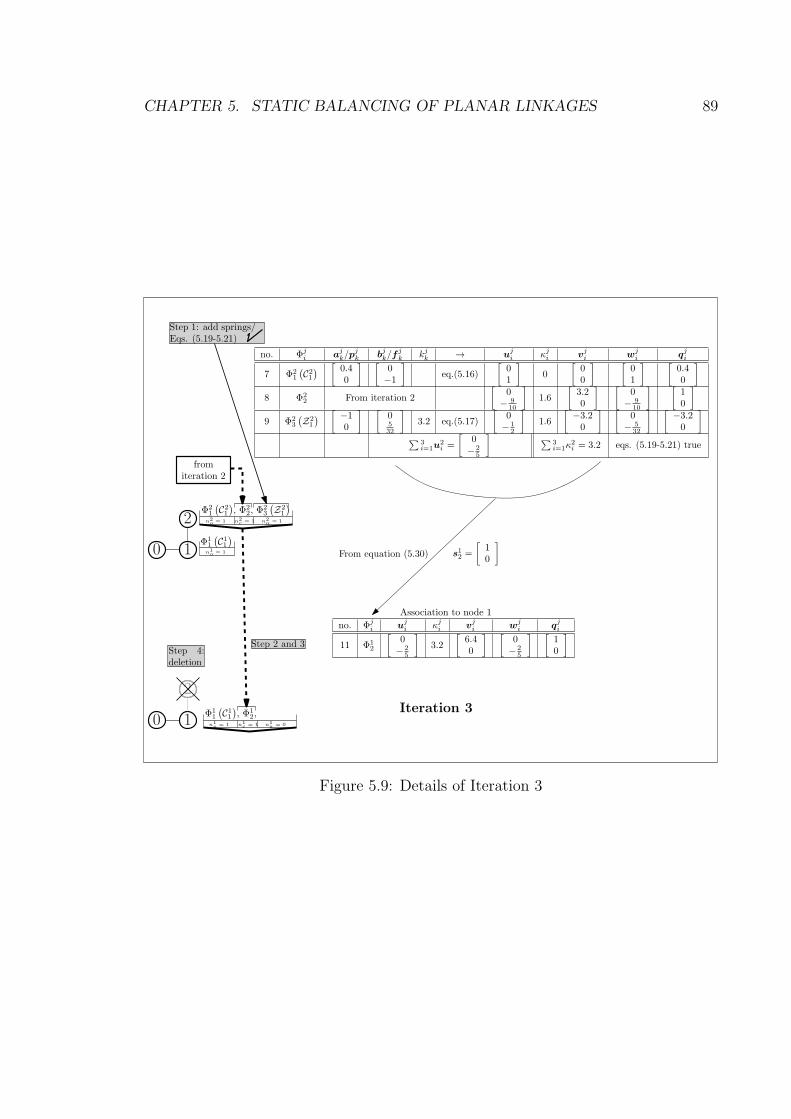
CHAPTER 5. STATIC BALANCING OF PLANAR LINKAGES 89
fromiteration 2
Step 1: add springs/Eqs. (5.19-5.21)
no. Φji a
jk/p
jk b
jk/f
jk k
jk → u
ji κ
ji v
ji w
ji q
ji
7 Φ2
1
(
C2
1
)
[
0.40
] [
0−1
]
eq.(5.16)
[
01
]
0
[
00
] [
01
] [
0.40
]
8 Φ2
2From iteration 2
[
0−
9
10
]
1.6
[
3.20
] [
0−
9
10
] [
10
]
9 Φ2
3
(
Z2
1
)
[
−10
] [
05
32
]
3.2 eq.(5.17)
[
0−
1
2
]
1.6
[
−3.20
] [
0−
5
32
] [
−3.20
]
∑
3
i=1u2
i =
[
0−
2
5
]
∑
3
i=1κ2
i = 3.2 eqs. (5.19-5.21) true
no. Φji u
ji κ
ji v
ji w
ji q
ji
11 Φ1
2
[
0−
2
5
]
3.2
[
6.40
] [
0−
2
5
] [
10
]
s12=
[
10
]
From equation (5.30)
Association to node 1
Iteration 3
2
10
n2o
= 1 n2a
= 1n2c
= 1
Φ2
1
(
C2
1
)
, Φ2
2, Φ2
3
(
Z2
1
)
n1o
= 1
Φ1
1
(
C1
1
)
2
10n1o
= 1 n1a
= 0n1c
= 1
Φ1
1
(
C1
1
)
, Φ1
2,
Step 4:deletion
2
Step 2 and 3
Figure 5.9: Details of Iteration 3

CHAPTER 5. STATIC BALANCING OF PLANAR LINKAGES 90
fromiteration 3
Iteration 4
Step 4:deletion
Step 2 and 3
1 n1o
= 1 n1a
= 0n1c
= 1
Φ1
1
(
C1
1
)
, Φ1
2,
0
1
0 n0c
= 1
Φ0
1
Step 1:springs unnecessary/eqn. (5.23-5.24)of propn. 1 aresatisfied as it is.
A constant(from propn. 1)Hence it is associated withthe root
no. Φji a
jk/p
jk b
jk/f
jk k
jk → u
ji κ
ji v
ji w
ji q
ji
10 Φ1
1
(
C1
1
)
[
0.40
] [
0−1
]
eq.(5.16)
[
01
]
0
[
00
] [
01
] [
0.40
]
11 Φ1
2s12=
[
10
]
eq.(5.30)
[
0−
2
5
]
3.2
[
6.40
] [
0−
2
5
] [
10
]
eqs. (5.23-5.24) is true with r1 =
[
00
]
Figure 5.10: Details of Iteration 4

CHAPTER 5. STATIC BALANCING OF PLANAR LINKAGES 91
x0
y0
y1
1
y2
y3
x2
y4
x4
0
2
3
4
C1
1C2
1
C3
1
C4
1
Z4
1
Z4
2
Z3
1
Z2
1
Figure 5.11: Statically balanced gravity-loaded serial 4R linkage.
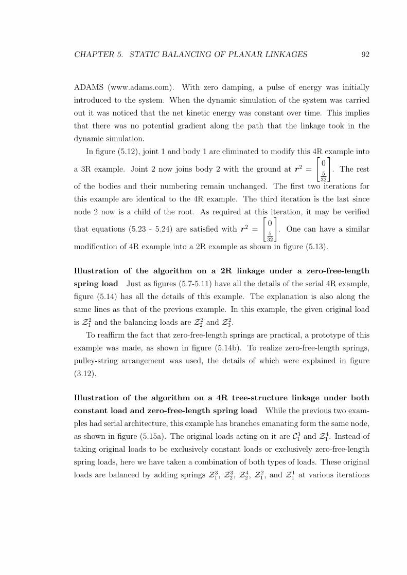
CHAPTER 5. STATIC BALANCING OF PLANAR LINKAGES 92
ADAMS (www.adams.com). With zero damping, a pulse of energy was initially
introduced to the system. When the dynamic simulation of the system was carried
out it was noticed that the net kinetic energy was constant over time. This implies
that there was no potential gradient along the path that the linkage took in the
dynamic simulation.
In figure (5.12), joint 1 and body 1 are eliminated to modify this 4R example into
a 3R example. Joint 2 now joins body 2 with the ground at r2 =
[
0532
]
. The rest
of the bodies and their numbering remain unchanged. The first two iterations for
this example are identical to the 4R example. The third iteration is the last since
node 2 now is a child of the root. As required at this iteration, it may be verified
that equations (5.23 - 5.24) are satisfied with r2 =
[
0532
]
. One can have a similar
modification of 4R example into a 2R example as shown in figure (5.13).
Illustration of the algorithm on a 2R linkage under a zero-free-length
spring load Just as figures (5.7-5.11) have all the details of the serial 4R example,
figure (5.14) has all the details of this example. The explanation is also along the
same lines as that of the previous example. In this example, the given original load
is Z21 and the balancing loads are Z2
2 and Z23 .
To reaffirm the fact that zero-free-length springs are practical, a prototype of this
example was made, as shown in figure (5.14b). To realize zero-free-length springs,
pulley-string arrangement was used, the details of which were explained in figure
(3.12).
Illustration of the algorithm on a 4R tree-structure linkage under both
constant load and zero-free-length spring load While the previous two exam-
ples had serial architecture, this example has branches emanating form the same node,
as shown in figure (5.15a). The original loads acting on it are C31 and Z4
1 . Instead of
taking original loads to be exclusively constant loads or exclusively zero-free-length
spring loads, here we have taken a combination of both types of loads. These original
loads are balanced by adding springs Z31 , Z
32 , Z
42 , Z
21 , and Z1
1 at various iterations

CHAPTER 5. STATIC BALANCING OF PLANAR LINKAGES 93
x0
y0
2
C2
1y2
3
4
Z4
2
Z4
1
C4
1
C3
1
Z3
1
y3
y4
x4
0
r2=
[
05
32
]
Figure 5.12: Statically balanced serial 3R linkage

CHAPTER 5. STATIC BALANCING OF PLANAR LINKAGES 94
x0
y0
3
y3
x3
y4
x4
Z4
1
Z4
2
C4
1
C3
1
4
0
r3 =
[
015
32
]
Figure 5.13: Statically balanced serial 2R linkage

CHAPTER 5. STATIC BALANCING OF PLANAR LINKAGES 95
Z2
1
Z2
2
Z2
3
2
1
0
Φ21
(
Z21
)
, Φ22
(
Z22
)
, Φ23
(
Z23
)
n2o
= 1 n2a
= 2
Step1: add springsEqs. (5.19-5.21)
2
1
0
Φ11
n1c
= 1
Step 4:Deletion
Steps 2 and 3
1
0Φ01
n0c
= 1
Step 4:Deletion
Step1:Eqs. (5.22-5.23)No extra springs
Steps 2 and 3
Constant fromproposition 1
Iteration 1
Iteration 2
x2
x1y
0
no. Φji a
j
k bj
k kj
k → uji κ
ji v
ji w
ji q
ji
1 Φ2
1
(
Z2
1
)
[
50
] [
1212
]
1 eq.(5.17)
[
−12−12
]
0.5
[
50
] [
−12−12
] [
50
]
2 Φ2
2
(
Z2
2
)
[
50
] [
−12−12
]
1 eq.(5.17)
[
1212
]
0.5
[
50
] [
1212
] [
50
]
3 Φ2
3
(
Z2
3
)
[
−50
] [
00
]
2 eq.(5.17)
[
00
]
1
[
−100
] [
00
] [
−100
]
∑
3
i=1u2
i =
[
00
]
∑
3
i=1κ3
i = 2 eqs. (5.19-5.21) true
4 Φ1
1 s1
2 =
[
10
]
eq.(5.30)
[
00
]
2
[
200
] [
00
] [
50
]
eqs. (5.23-5.24) is true with r1 =
[
00
]
(c)
(a)
(b)
Figure 5.14: Details of static balance of a 2R linkage under spring load
in the iterative algorithm. A pictorial depiction of the iterations on this linkages is
given in figure (5.15b). All the remaining details are given in the table of the same
figure.
To verify the static balance, θs of bodies 1, 2, 3 and 4 are varied in the following
form: θ1 = π4+ π sin (2πt), θ2 = π
12+ π sin (2πt), θ3 = π
1.7+ π sin (2πt), θ4 = π
1.3+
π sin (2πt). The potential energy variation of original loads C31 and Z4
1 as well as the
balancing loads, i.e., Z31 , Z
32 , Z
42 , Z
21 , and Z1
1 , are plotted in figure (5.16). The sum
of all these variations is also plotted and it has turned out to be a constant. This
verifies the static balance.

CHAPTER 5. STATIC BALANCING OF PLANAR LINKAGES 96
1
2
34
X
Y
0
Z31
Z32
Z41
Z42
Z21
Z11
no. Φji a
jk/p
jk b
jk/f
jk k
jk → u
ji κ
ji v
ji w
ji q
ji
1 Φ4
1
(
Z4
1
)
[
10
] [
7
23
2
]
1 eq.(5.17)
[
−7
2
−3
2
]
1
2
[
10
] [
−7
2
−3
2
] [
10
]
2 Φ4
2
(
Z4
2
)
[
−10
] [
7
23
2
]
1 eq.(5.17)
[
−7
2
−3
2
]
1
2
[
−10
] [
−7
2
−3
2
] [
−10
]
∑
2
i=1u4
i =
[
−7−3
]
∑
2
i=1κ4
i = 1 eqs. (5.19-5.21) true
3 Φ3
1
(
C3
1
)
[
10
] [
0−1
]
eq.(5.16)
[
01
]
0
[
00
] [
01
] [
10
]
4 Φ3
2
(
Z3
1
)
[
1
2
0
] [
1
2
3
]
1 eq.(5.17)
[
−1
2
−3
]
1
2
[
1
2
0
] [
−1
2
−3
] [
1
2
0
]
5 Φ3
3
(
Z3
2
)
[
−1
2
0
] [
1
2
1
]
1 eq.(5.17)
[
−1
2
−1
]
1
2
[
−1
2
0
] [
−1
2
−1
] [
−1
2
0
]
∑
3
i=1u3
i =
[
−1−3
]
∑
3
i=1κ3
i = 1 eqs. (5.19-5.21) true
7 Φ2
1s23=
[
−13
5
]
eq.(5.30)
[
−1−3
]
1
[
−26
5
] [
−1−3
] [
−13
5
]
8 Φ2
2s24=
[
13
5
]
eq.(5.30)
[
−7−3
]
1
[
26
5
] [
−7−3
] [
13
5
]
9 Φ2
3
(
Z2
1
)
[
0−
6
5
] [
24
]
2 eq.(5.17)
[
−4−8
]
1
[
0−
12
5
] [
−2−4
] [
0−
12
5
]
∑
3
i=1u2
i =
[
−12−14
]
∑
3
i=1κ2
i = 3 eqs. (5.19-5.21) true
10 Φ1
1s12=
[
10
]
eq.(5.30)
[
−12−14
]
3
[
60
] [
−12−14
] [
10
]
11 Φ1
2
(
Z1
1
)
[
1
2
0
] [
5
41
6
]
12 eq.(5.17)
[
−15−2
]
6
[
60
] [
−5
4
−1
6
] [
60
]
eqs. (5.23-5.24) is true with r1 =
[
13
85
4
]
C31
0
1
2
3 4Φ4
1
(
Z4
1
)
, Φ4
2
(
Z4
2
)
n4o
= 1 n4a
= 1
Φ3
1
(
C3
1
)
, Φ3
2
(
Z3
1
)
, Φ3
3
(
Z3
2
)
n3o
= 1 n3a
= 2
0
1
2Φ2
1, Φ2
2, Φ2
3
(
Z2
1
)
n2c
= 2 n2a
= 1
Iteration 1
Step1: add springsEqs. (5.19-5.21)
Step1: add springsEqs. (5.19-5.21)
Step1: add springsEqs. (5.19-5.21)
Step 2 & 3Step 2 & 3
0
1Φ1
1, Φ1
2
(
Z1
1
)
n1c
= 1 n1a
= 1
Iteration 2
Step1: add springsEqs. (5.23-5.24)
Step 2 & 3
0 Φ0
1
A constant
Iteration 2
Step 2 & 3
(a)
(b)
Original loads
Figure 5.15: Details of static balance of a 4R tree-structure linkage under a constantload and a spring load
5.4.3 Static balancing of any revolute-jointed linkages with
any kind of zero-free-length spring and constant load
interaction within the linkage
In the static balancing method for linkages provided in Section 5.4.2, other than
the fact that the linkage to be balanced has to be revolute-jointed and that load
interactions are of zero-free-length spring or constant loads, there were two more
restrictions:

CHAPTER 5. STATIC BALANCING OF PLANAR LINKAGES 97
-5
0
5
10
15
20
25
30
35
0 0.2 0.4 0.6 0.8 1
C3
1
Z4
1
Z3
1Z3
2
Z4
2
Z2
1
Z1
1
Net Potential Energy
t −→
PE
Figure 5.16: Potential Energy variation of spring loads, constant loads, and their sum
1. It should be possible to consider that the loads on all the bodies are exerted by
a common reference body (or frame) of the linkage.
2. The linkage should have a tree-structure (i.e., without closed loops).
When the first restriction is violated, as in figure (5.17a), it is always possible
to break the load interactions into a superposition of several load sets with each set
complying with the first restriction. For example, the load interaction in figure (5.17a)
is broken into two load sets in figures (5.17b) and (5.17c). The reference body in
each of these sets is indicated by an asterisk symbol (*) in their respective figures.
Furthermore, in a load set, if there are closed loops, then the closed loops can be
broken by relaxing certain joint constraints. Figures (5.17c) and (5.17d) illustrate
breaking of closed loops in figures (5.17b) and (5.17c), respectively. With closed

CHAPTER 5. STATIC BALANCING OF PLANAR LINKAGES 98
Breaking closed loops
Breaking load interactions
+
*
*
(a) (b) (c)
(c) (d)
Joint relaxed
Joint relaxed
Figure 5.17: Breaking a problem as a superposition of several problem with eachproblem being static balance of revolute-jointed tree-structured linkage with loadsexerted by the root body
loops broken, each of the load sets comply with the two restrictions and they can be
statically balanced by adding balancing loads as per Section 5.4.2.
Once each of the load sets is balanced, the joint constraints that were relaxed
for breaking closed loops can be reimposed without disturbing the static balance. In
other words, when the potential energy that is a function of the configuration space is
a constant, it remains as the constant even when the configuration space is restricted
(due to re-attachment of the broken joints).
Once the constraints are reimposed, the linkages in all the load sets are the same
as the original linkage and the loads on all the sets can be superposed. Since each load
set is in static balance, the superposition is also in static balance. In other words, the
sum of several constant potential energy functions due to several load sets is also a

CHAPTER 5. STATIC BALANCING OF PLANAR LINKAGES 99
constant. This superposition contains all the original loads on the given linkage. The
remnant loads in this superposition are the additional loads that balance the original
loads. In this way, additional loads that statically balance any revolute-jointed linkage
with zero-free-length spring and constant load interactions between the bodies of the
linkage can always be found. An example is presented next to illustrate this.
A numerical example
Figure (5.18a) shows a linkage which is the same as that in figure (5.15) except for
an additional zero-free-length spring between the three-lobed body and the left-most
body. Unlike in figure (5.15), where the ground can be considered as the reference
body that exerts loads on all the bodies, in figure (5.18a) it is not possible to find a
single reference body that exerts loads on all the bodies. Hence the loads are split
into two sets as in figures (5.18b) and (5.18c). The first set shown in figure (5.18b)
is the same as that in figure (5.15) whose balancing loads are already found using
iterative algorithm detailed in figure (5.15).
In the second set shown in figure (5.18c), the three-lobed body is treated as the
reference frame. The bodies are labelled accordingly with the number 0 assigned to
the reference body. The only spring in the figure is labelled as Z11 . In this figure,
there is only one load interaction, which is between body 1 and the reference frame.
Further, body 1 can be considered as lever on the reference body. An extra spring Z12
between body 1 and 0 is added, the details of which are given figure (5.19), to satisfy
the conditions of static balance of a lever (equations (5.10) – (5.11)). With this the
second load set is balanced.
The balanced first and second load sets are shown in figures (5.18d) and (5.18e),
which are further superposed as in figure (5.18f) to obtain the balancing solution to
the original load set shown in (5.18a).
5.5 A note on prismatic joint
In Section 5.3, it was noted that by merely adding springs, the dependency of a body’s
potential energy on r cannot be annihilated. As shown in the later sections, in the
CHAPTER 5. STATIC BALANCING OF PLANAR LINKAGES 100
+
+
0
1
2
34
Set 1 Set 2C31
Z41
C31
Z41
0
1
34Z3
1
Z32
Z42
Z21
Z11
2
0
1
Reference body
The ground
Reference body
2
3
4
Z11
4
3
2
0
1
Z11
Z12
Splitting original loads
Superposition of balanced load sets
Static balancingSee figure (5.15)
Static balancing
See figure (5.19)
(a) (b) (c)
(e)(d)(f)
Figure 5.18: Static balance of a tree-structured linkage with inter-body load interac-tions
case of the body having a revolute joint with another body, this dependency on r
can be transmitted as a dependency on the coordinates of the other body when r
points to the common point of the revolute joint. This allows us to think that the
dependency of the potential energy on r is conceptually removed by transmission.
The static balancing strategy outlined in this chapter is based on carrying out this
transmission in a cascading manner.
If the body has a prismatic joint instead of the revolute joint, there is no scope
for the conceptual removal by transmission since r cannot be expressed in terms of
the coordinates of the other body. This un-annihilated potential energy dependence
of r implies that in a tree-structured chain, if there is a prismatic joint, there is no
way static balance can be achieved by merely adding springs. In such situations,
it is necessary to add revoluted-jointed chain as auxiliary chain and carry out the

CHAPTER 5. STATIC BALANCING OF PLANAR LINKAGES 101
4
0
1
Z11
Z12
X
Y
Reference frame
Body 1 is a lever with respect to body 0[
−1
2
3
10
]T
[
3
40]T
[
−3
40]T
Spring details
a
Z12
[
3
40]T
b
[
−1
2
3
10
]T
Z11
[
−3
40]T
[
−1
2
3
10
]T
k
1
1
r =[
−1 35
]T
is a constant
k (r − b)T a k (r − b)T R(
π
2
)
a
3
8
−3
8
−9
40
+ 9
40
Equations (5.10) and (5.11) satisfied
Figure 5.19: Balancing the lever lever loads in the second load set of figure (5.18)
cascading transmission through this auxiliary chain. In closed loop linkages, such
auxiliary chains may be inherently present as in the case of a slider crank linkage
which can be thought as a 3R chain closing its loop with a prismatic joint.
Summary
• We presented a technique to statically balance any planar revolute-jointed link-
age having zero-free-length spring and constant load interactions between the
bodies of the linkage.
• The technique involves only addition of zero-free-length springs but not any
extra link, unlike spring-aided perfect static balancing techniques currently in
the literature.
• The technique relies on a recursive relation to iteratively remove the dependence
of the potential energy on the configuration variables of the bodies of the linkage.
• Recognizing the recursive relation along with the minimal conditions that enable
it constitutes the contribution of this chapter.
Chapter 6
Static balancing of spatial linkages
without auxiliary bodies
Overview
• Just as a recursive relation in the planar case enabled an iterative algorithm,
there is a recursive relation in the spatial case also.
• The recursive relation holds when the loads are constant loads and/or zero-free-
length spring loads and the joints are revolute and/or spherical joints.
• Similar to the planar case, even though the iterative algorithm works on a tree-
structured linkage, extension to an arbitrary linkage is straightforward.
6.1 Introduction
The results of Chapter 5 hinged on Proposition 2, which was recursively applied in
the iterative algorithm of Section (5.4.2). If we can have a similar proposition in the
spatial case, then we can have an iterative static balancing algorithm for spatial case
also. The features of the proposition that allowed its recursive application are:
• Feature 1: The allowable loads on a body, say body j, should have a potential
energy that belongs to a class of functions of configuration variables of the body.
102

CHAPTER 6. STATIC BALANCING OF SPATIAL LINKAGES 103
Let the class of functions be represented by χ(j). In Section 5.4.2, the allowable
loads are zero-free-length spring and constant loads, and the class of functions
are as in equation (5.15).
• Feature 2: A joint between two bodies, say body j and body l, should provide
a relation between configuration variables of j and l that can be used to express
the sum of a set of functions in χ(l) as a function in χ(j). This is essential for
steps 1 to 3 of the iterative procedure in Section 5.4.2.
For spatial linkages, a class of functions and the joints having the two features are
presented next.
6.2 The class of functions in feature 1
If a body in space has its configuration with respect to a reference frame defined by r
and R, the position vector and rotation matrix of the local frame with respect to the
global frame, then the potential energy of a constant load and a positive-stiffness zero-
free-length spring and a general form of potential energy function that can express
potential energies of both constant load and zero-free-length spring loads are:
PEc = (−f)T r + (−f)T Rp (6.1)
PEs = (−kb)T r + (−kb)T Ra+ rTR (ka) +k
2rTr
+k
2
(aTa+ bTb
), k > 0 (6.2)
Φ = uTr +wTRq + rTRv + κrTr + c, κ ≥ 0 (6.3)
The derivation and the notation used in equations (6.1), (6.2), and (6.3) are the same
as those in equations (5.1), (5.6), and (5.15), respectively, except that they are all
spatial quantities now.
The class of functions referred in feature 1 would be the functions of the form
given in equation (6.3). We do not consider a broader class of functions that includes
potential energies of positive zero-free-length springs since the extra terms associated

CHAPTER 6. STATIC BALANCING OF SPATIAL LINKAGES 104
with positive-free-length spring (see equation (5.8)) cannot be balanced out for the
reasons same as those given in Appendix C.
It may be noted that R, unlike in planar case, is not a function of just a single
variable. Among many possibilities, R may be considered as a function of three Euler
angles. We use body fixed Z −X ′ − Z ′′ system of Euler angles with the three angles
represented as α, β and γ so that R becomes
R =
c1c3 − s1c2s3 −c1s3 − s1c2c3 s1s2
s1c3 + c1c2s3 −s1s3 + c1c2c3 −c1s2
s2s3 s2c3 c2
(6.4)
where c1 = cosα, s1 = sinα, c2 = cos β, s2 = sin β, c3 = cos γ, and s3 = sin γ.
Just as in table 5.1, the function in equation (6.3) can be expressed as a linear
combination a finite number of linearly independent functions where each function is
a function of r and {α, β, γ}. The functions, which are also a basis for the function
in equation (6.3), and the corresponding coefficients are presented in table 6.1.
6.3 Joints that can potentially satisfy feature 2
Consider the following proposition, which is along the same same lines as in Section
5.3. This proposition helps us to narrow down on spatial joints that can potentially
have feature 2, as discussed after the proof of the proposition.
Proposition 3. For a given set of functions of the form
Φi = rTui +wTi Rqi + rTRvi + κir
Tr + ci,
κi ≥ 0 and i = 1 · · ·nf (6.5)
that are associated with a rigid-body defined by r and R,
1. the net sum of these functions along with the potentials of one or more positive-
stiffness zero-free-length springs cannot be independent of r.

CHAPTER 6. STATIC BALANCING OF SPATIAL LINKAGES 105
Table 6.1: The potential in the general form shown in figure (6.3), can be expressedas a linear combination of the basis functions shown in the table. Each basis functionin the table is a function of translational variable r and the Z-X-Z Euler angle α, βand γ
No. Basis functions Coefficient1 rx ux2 ry uy3 rz uz4 r2x + r2y + r2z κ
5 rx(c1c3 − s1c2s3) + ry(s1c3 + c1c2s3) + rz(s2s3) vx6 rx(−c1s3 − s1c2c3) + ry(−s1s3 + c1c2c3) + rz(s2c3) vy7 rx(s1s2) + ry(−c1s2) + rz(c2) vz8 c1c3 − s1c2s3 wxqx9 s1c3 + c1c2s3 wyqx10 s2s3 wzqx11 −c1s3 − s1c2c3 wxqy12 −s1s3 + c1c2c3 wyqy13 s2c3 wzqy14 s1s2 wxqz15 −c1s2 wyqz16 c2 wzqz17 1 c

CHAPTER 6. STATIC BALANCING OF SPATIAL LINKAGES 106
2. it is possible to find a finite set of positive-stiffness zero-free-length spring loads
such that the net sum of the functions and potentials of springs is independent
of orientation variable R.
Proof. Let (ki,ai, bi), ki > 0 and i = 1 · · ·na be any set of na ≥ 1 zero-free-length
spring loads on the rigid-body. Their potential energy can be written in the general
form shown in equation (6.3), where the parameters of the general form, corresponding
to na springs, are represented as {ui, wi, qi, vi, κi, ci}, κi > 0, i = nf+1 · · ·nf+na.
The net sum of the given functions and the potential energies of the springs take the
following form.
nf+na∑
i=1
Φi = rT
nf+na∑
i=1
ui +
nf+na∑
i=1
wTi Rqi+
rTR
nf+na∑
i=1
vi + rTr
nf+na∑
i=1
κi +
nf+na∑
i=1
ci
(6.6)
The coefficient of rTr in equation (6.6) is a non-zero positive number since κi ≥ 0 for
i = 1 · · ·nf , κi > 0 for i = nf +1 · · ·nf +na and na ≥ 1. Hence, the net sumnf+na∑
i=1
Φi,
i.e., the net sum of functions along with the potentials cannot be independent of r.
Thus the first part of the proposition is proved.
Now, consider the second part of the proposition. The net sum is also a linear
combination of the basis functions given in table 6.1 with the corresponding coeffi-
cients being the same as in the table except that the coefficients are subscripted with
i and summed over i from 1 to nf + na. The net sum is independent of orientation
if and only if all the coefficients of the basis functions that are dependent on α or β
or γ are zero. The coefficients of the basis function nos. 5, 6 and 7 in table 6.1 being
constrained to zero can be compactly written as
nf+na∑
i=1
vi = 0 (6.7)
The elements in the rows 8 – 16 in the right most column of table 6.1 are actually

CHAPTER 6. STATIC BALANCING OF SPATIAL LINKAGES 107
nine elements of the matrix qwT . Hence, the coefficients for the net sum of the basis
function nos. 8–16 in table 6.1 being constrained to zero can be written as
[
q1 · · · qnf+na
] [
w1 · · · wnf+na
]T
= 0 (6.8)
It is shown in Appendix E that no matter what the parameters {ui, wi, qi, vi, κi, ci}
for i = 1 · · ·nf are, there are always four zero-free-length springs having such a set
of parameters (ki,ai, bi), ki > 0 and i = 1 · · · 4 that the equations (6.7) and (6.8) are
satisfied. Hence, the second part of the proposition is also true.
If a joint should have feature 2, then the joint should transform the dependence
on r, which cannot be balanced out as per the proposition, to dependence on the
configuration variables of another body between which the joint exists. In other
words, r, i.e., position vector of local origin on the body, should be a function solely
of the configuration variables of the other body. Among the basic joints, such a thing
is possible only if the other body is connected to the body by a revolute or spherical
joint at the origin. Thus, spherical joints and revolute joints can potentially have
feature 2 and we next prove that they indeed have.
From here onwards, we deal with more than one body and each body is assigned a
distinct number. Further, if quantities such as r, R, ui, ki are associated with body
j, then the corresponding symbols are superscripted with j. With this, quantities
associated with different bodies can be distinguished from one another.
6.4 Spherical joint has feature 2
Here is the proposition with its proof that essentially says that for the class of func-
tions given in equation (6.3), the spherical joint has feature 2 under certain conditions.
Proposition 4. For a given set of functions
Φli = rlTul
i +wli
TRlql
i + rlTRlvli + κlir
lTrl + cli,
κli ≥ 0 and i = 1 · · ·nl(6.9)

CHAPTER 6. STATIC BALANCING OF SPATIAL LINKAGES 108
that is associated with body l, if:
Condition 1: There is a spherical joint between body j and body l such that a point
fixed to body j is coincident with the local origin of body l. Let the local coordi-
nates of the point on body j be sjl .
Condition 2: Equations (6.7) and (6.8) are satisfied with nf + na being nl.
thennl∑
i=1
Φli = rjTu
ji +w
ji
TRjq
ji + rjTRjv
ji + κjir
jTrj (6.10)
where
uji =
nl∑
i=1
uli, w
ji =
nl∑
i=1
uli, q
ji = s
jl ,
vji = 2sjl
nl∑
i=1
κli, κji =nl∑
i=1
κli
(6.11)
Proof. The equation form of condition 1 is
rj +Rjsjl = rl (6.12)
The equations referred in condition 2 are the necessary and sufficient constraints
to make the net sumnl∑
i=1
independent of Rl, as shown in the proof of proposition 3.
Hence, under condition 2, in the expression fornl∑
i=1
Φli, the Rl dependent terms can
be omitted as shown next
nl∑
i=1
Φli = rlT
nl∑
i=1
uji + rlTrl
nl∑
i=1
κli (6.13)
nl∑
i=1
Φli represents potential energy and our interest is in the gradient of the potential
energy with respect to the configuration variables. Hence, the constant terms, which

CHAPTER 6. STATIC BALANCING OF SPATIAL LINKAGES 109
do not affect gradients, are inconsequential. This is the reason for omitting constant
terms as well in equation (6.13).
On the same lines as in proposition 2, substitution for rl from equation (6.12) into
equation (6.13), simplification and omission of the constant term leads to equations
(6.10) and (6.11).
6.5 Revolute joint has feature 2
Proposition 4 holds for revolute joints as well. However, the fact that in a revolute
joint, a line, rather than a point, fixed to two bodies are coincident allows us to make
condition 2 of proposition 4 less stringent as shown next.
Proposition 5. For given a set of functions
Φli = rlTul
i +wli
TRlql
i + rlTRlvli + κlir
lTrl + cli,
κli ≥ 0 and i = 1 · · ·nl(6.14)
that is associated with body l, if:
Condition 1: There is a revolute joint between body j and body l such that a point
fixed to body j is coincident with the local origin of body l and a unit vector fixed
to body j is always parallel to local z-axis of body l. Let the local coordinates of
the point on body j be sjj and the unit vector fixed to body j in local frame of
reference be kj
l .
Condition 2: Following equations are satisfied.
nl∑
i=1
vli = 0 (6.15)
[
ql1 · · · ql
nl
] [
wl1 · · · wl
nl
]T
= 0 (6.16)
where v = [vx vy]T and q = [qx qy]
T .

CHAPTER 6. STATIC BALANCING OF SPATIAL LINKAGES 110
thennl∑
i=1
Φli = Φj
i + Φji+1 (6.17)
where φji and Φj
i+1 are functions of the form in equation (6.14) but associated with
body j. uji , w
ji , q
ji , v
ji , κ
ji are as given in equation (6.11), and u
ji+1, w
ji+1, q
ji+1, v
ji+1,
κji+1 are as given next.
uji+1 = 0, w
ji+1 =
nl∑
i=1
qlz,iwli, q
ji+1 = k
j
l
vji+1 = k
j
l
nl∑
i=1
vlz,i, κji = 0
(6.18)
Proof. From condition 1 of the proposition, we have
rj +Rjsjl = rl (6.19)
Rjkj
l = Rl[0 0 1]T = [sl1sl2 − cl1s
l2 cl2]
T (6.20)
What equation (6.20) says is that terms sl1sl2, −c
l1s
l2 and cl2 can be considered as
functions of configuration variables of body j. Hence, for the net sum, it is not
necessary to constrain the coefficients of basis functions involving only these functions
and rl (function nos. 7, 14, 15 and 16 in table 6.1) to zero. Instead, one can transform
the dependence on these function and rl to dependence on the configuration variables
of body j using equations (6.19) and (6.20). This is the reason for truncating v and
q in equations (6.15) and (6.16). This truncation omits coefficients corresponding to
basis function nos. 7, 14, 15 and 16 in table 6.1.
The contribution of basis functions nos. 1, 2, 3, and 4 (as in table 6.1), after
transformation to configuration of body j, is already written in equations (6.10) and
(6.11). Φji in equation (6.17) represent the same. The contribution from basis function
no.7 is
rlT [sl1sl2 − cl1s
l2 cl2]
T
nl∑
i=1
vlz,i (6.21)

CHAPTER 6. STATIC BALANCING OF SPATIAL LINKAGES 111
The contribution from basis function nos. 14, 15 and 16 is
nl∑
i=1
qlz,iwli
T
[sl1sl2 − cl1s
l2 cl2]
T (6.22)
Substitution for rl and [sl1sl2 − cl1s
l2 cl2] from equations (6.19) and (6.20) into the
sum of expressions (6.21) and (6.22), followed by simplification, yields
rjTRj
kj
l
nl∑
i=1
vlz,i
+
nl∑
i=1
qlz,iwli
T
Rjkj
l (6.23)
This term is represented as Φli+1 in equation (6.17) and is the contribution from basis
function nos. 7, 14, 15 and 16, after transformation to configuration variables of body
j. The reason for not combining two functions on the right hand side of equation
(6.17) into one is that the terms wji
TRjq
ji and wjT
i+1Rjq
ji+1 cannot be combined.
6.6 Algorithm to synthesize static balancing so-
lution of a spatial revolute/spherical-jointed
tree-structured linkage having zero-free-length
spring and/or gravity loads exerted by a ref-
erence link
This is along the same lines as in Section 5.4.2.
Preparatory steps
1. Assign the reference body as the root node of the tree-structure.
2. If the joint between a body and its parent body is a revolute joint, then choose
the local frame of reference of the body such that the z-axis of the local frame

CHAPTER 6. STATIC BALANCING OF SPATIAL LINKAGES 112
is aligned along the axis of the revolute joint. If the joint between a body and
its parent is spherical joint, then choose the local frame of reference of the body
such that the origin of the local frame coincides with the center of the spherical
joint.
3. Give this tree-structure with the given constant and zero-free-length spring loads
as an input to the following iterative procedure.
Iterative procedure
• Entry condition: If the tree-structure contains only the root node, then exit
from the iterative procedure. Otherwise, proceed to step 1.
• Step 1: For every body/node, there are two kinds of potential energy functions
associated with it. One kind is due to loads acting on the body and the other
kind is due to the association that happened in step 3 of previous iterations.
From equations (5.16-5.17) (which holds for spatial case also), proposition 4
and proposition 5, respectively, both kinds of potential energy are of the form
given in equation (6.3) where r and R are configuration variables of the body.
For every terminal node l of the tree-structure, add extra nla zero-free-length
springs such that the potential energy functions due to 1) nlo original loads on
the body, 2) nlc associations that happened with node l in step 3 of previous
iterations, and 3) nla extra zero-free-length spring loads satisfy condition 2 of
proposition 4 in the case of spherical joint and condition 2 of proposition 5 in
the case of revolute joint. Appendix E shows that such a thing is possible.
• Step 2: Expressnlo+nl
c+nla∑
i=1
Φli as function of configuration variable of the parent
link. This is possible since condition 1 (because of preparatory steps), condi-
tion 2 (because of step 1) of proposition 4 in the case of spherical joint and
proposition 5 in case revolute joint are satisfied.
• Step 3: Associatenlo+nl
c+nla∑
i=1
Φli with the parent link of l and for energy conser-
vation, disassociate Φli, i = 1 · · ·nl
o + nlc + nl
a from node l.

CHAPTER 6. STATIC BALANCING OF SPATIAL LINKAGES 113
• Step 4: With all the potential energy functions disassociated from node l to
its parent, delete this terminal node l.
• Iterator: Once steps 1 to 4 are completed, a new trimmed tree-structure results
where the parents of the nodes deleted in step 4 has additional potential energy
functions associated with them. Follow this iterative procedure again with this
trimmed tree-structure as the input.
The arguments that this algorithm indeed leads to static balance is also the same as
that in Section 5.4.2. The distinct cases (a) and (b) of Section 5.4.2 exist in spatial
case also. We indicate case (b) in the last iteration of the following example.
6.6.1 Illustrative example
Figure (6.1-(ii)) shows a six degree-of-freedom spatial linkage consisting of four bodies
that are serially connected to the ground. Starting from the ground, the first three
joints are revolute and the last joint is spherical. The architecture is the same as
PUMA robot except that the wrist of the PUMA robot is replaced by a spherical
joint. Starting from 0 for the ground, the bodies are serially numbered as 1, 2, 3
and 4. Bodies 2, 3 and 4 are under the influence of constant loads C41 , C
31 , and C2
1 as
shown in figure (6.1). The constant loads are due to gravitational force on the bodies.
In order to statically balance this spatial linkage, we follow the iterative algorithm
described in Section 6.6.
Local frames of reference are assigned as per the preparatory steps of the algo-
rithm. A D-H table as well as Sjl and k
j
l parameters describing relative position of
the frames are given in tables (c) and (d) of figure (6.1). In the following iterative
procedure, six springs Z41 , Z
42 , Z
43 , Z
31 , Z
21 , and Z1
1 are added to balance the three
constant forces. Tables (a) and (b) of figure (6.1) provide parameters of the constant
forces as well as zero-free-length springs. Further, by comparing equations (6.1) and
(6.2) with equation (6.3), the potential energies in the generalized form for these
constant forces and zero-free-length springs are tabulated in table (e) of figure (6.1).
The generalized form of potential energies that are obtained in steps 2 and 3 of the

CHAPTER 6. STATIC BALANCING OF SPATIAL LINKAGES 114
0 1
2
3
4 Φ4
1
(
C4
1
)
, Φ4
2
(
Z4
1
)
, Φ4
3
(
Z4
2
)
, Φ4
4
(
Z4
3
)
Φ3
1
(
C3
1
)
Φ2
1
(
C2
1
)
Step 1 of iteration 1:Spring additionCond. 2 of prop. 4
0 1
2
3
4
Φ3
1
(
C3
1
)
, Φ3
2, Φ3
3
(
Z3
1
)
Φ2
1
(
C2
1
)
Step 4 of iteration 1Deletion of node 4
0 1
2
3
Φ2
1
(
C2
1
)
, Φ2
2, Φ2
3, Φ2
4
(
Z2
1
)
0 1
2
Φ1
1, Φ1
2, Φ1
3
(
Z2
1
)
Spring additionEqs. (6.24) and(6.25)
1
x0
y0z
0
2
34
x2
y2
z2
x1
y1z
1
x3
y3
z3
x3
y3
z3
C4
1
C3
1
C2
1
Z4
1
Z4
2
Z4
3
Z3
1
Z2
1
Z1
1
0 (Ground)
D-H parameters
i αi−1 ai−1 di θi
1 0 0 1.2 θ1
2 π
20 −0.175 θ2
3 0 0.6 0.075 θ3
4 −π
20.6 0 ∗ ∗ ∗
Further tranformation offrame 4 is described by 321body fixed euler angles: e
4
1,
e4
2, and e
4
3.
Sjl and k
jl parameters
S0
1
[
0.0 0.0 1.2]T
k0
1
[
0 0 1]T
S1
2
[
0.0 0.175 0.0]T
k1
2
[
0 −1 0]T
S2
3
[
0.6 0.0 0.075]T
k2
3
[
0 0 1]T
S3
4
[
0.6 0.0 0.0]T
Parameters of constant forces
Cji p
ji f
ji
C4
1
[
0.25 0.0 0.0]T [
0.0 0.0 −0.4]T
C3
1
[
0.2 0.0 0.0]T [
0.0 0.0 −0.9]T
C2
1
[
0.2 0.0 0.0]T [
0.0 0.0 −0.9]T
Parameters of zero-free-length springs
Zj
i aj
i bj
i kj
i
Z4
1
[
0.5 0 0]T [
0.7 0.1 0.4]T
1
Z4
2
[
−0.25 0.2 0]T [
0.7 0.1 0.2]T
1
Z4
3
[
−0.25 −0.2 0]T [
0.7 0.1 0.2]T
1
Z3
1
[
−0.2 0.0 0.05]T [
0.7 0.1 1
30
]T9
Z2
1
[
−0.2 0.0 0.025]T [
0.7 0.1 −1
24
]T36
Z1
1
[
0 −41
320−
301
240
]T [
0.7 0.1 −13
240
]T48
Parameters of potentials due to springs, constant forces and transformation cum association in steps 2 and 3
Φj
i uj
i qj
i wj
i vj
i κj
i
Φ4
1
(
C4
1
) [
0.0 0.0 0.4]T [
0.25 0.0 0.0]T [
0.0 0.0 0.4]T [
0.0 0.0 0.0]T
0
Φ4
2
(
Z4
1
) [
−0.7 −0.1 −0.4]T [
0.5 0 0]T [
−0.7 −0.1 −0.4]T [
0.5 0 0]T 1
2
Φ4
3
(
Z4
2
) [
−0.7 −0.1 −0.2]T [
−0.25 0.20 0]T [
−0.7 −0.1 −0.2]T [
−0.25 0.20 0]T 1
2
Φ4
4
(
Z4
3
) [
−0.7 −0.1 −0.2]T [
−0.25 −0.20 0]T [
−0.7 −0.1 −0.2]T [
−0.25 −0.20 0]T 1
2
Φ3
1
(
C3
1
) [
0.0 0.0 0.9]T [
0.2 0.0 0.0]T [
0.0 0.0 0.9]T [
0.0 0.0 0.0]T
0
Φ3
2 =4∑
i=1
Φ4
i
[
−2.1 −0.3 −0.4]T [
0.6 0.0 0.0]T [
−2.1 −0.3 −0.4]T [
1.8 0.0 0.0]T
1.5
Φ4
3
(
Z3
1
) [
−6.3 −0.9 −0.3]T [
−1.8 0.0 0.45]T [
−0.7 −0.1 −1
30
]T [
−1.8 0.0 0.45]T
4.5
Φ2
1
(
C2
1
) [
0.0 0.0 0.9]T [
0.0 0.0 0.9]T [
0.2 0.0 0.0]T [
0.0 0.0 0.0]T
0
Φ2
2 +Φ2
3=3∑
i=1
Φ3
i
[
−8.4 −1.2 0.2]T [
−8.4 −1.2 0.2]T [
0.6 0.0 0.075]T [
7.2 0.0 0.9]T
6[
0.0 0.0 0.0]T [
−0.315 −0.045 −0.015]T [
0.0 0.0 1.0]T [
0.0 0.0 0.45]T
0
Φ2
4
(
Z2
1
) [
−25.2 −3.6 1.5]T [
−0.7 −0.1 1
24
]T [
−7.2 0.0 0.9]T [
−7.2 0.0 0.9]T
18
Φ1
1 +Φ1
2=4∑
i=1
Φ2
i
[
−33.6 −4.8 2.6]T [
−33.6 −4.8 2.6]T [
0.0 0.175 0.0]T [
0.0 8.4 0.0]T
24[
0.0 0.0 0.0]T [
−63
40−
9
40
3
80
]T [
0 −1 0]T [
0 −2.25 0]T
0
Φ1
3
(
Z1
1
) [
−33.6 −4.8 2.6]T [
−0.7 −0.1 13
240
]T [
0.0 −6.15 −60.2]T [
0.0 −6.15 −60.2]T
24
(i) (ii)
(a)
(b)
(c) (d)
(e)
n4o
= 1 n4a
= 3
Step 2 of iteration 1:∑
= Φ3
2(as per eqn. 6.10)
Step 3 of iteration 1:association with node 3
Step 1 of iteration 2:Spring additionCond. 2 of prop. 5
n3o
= 1 n3c
= 1 n3a
= 1
Step 2 of iteration 2:∑
= Φ2
2+Φ2
3(as per eqn. 6.17)
Step 3 of iteration 2:association with node 2
Step 4 of iteration 2Deletion of node 3
n2o
= 1 n2c
= 2 n2a
= 1
Step 1 of iteration 3:Spring additionCond. 2 of prop. 5
Step 2 of iteration 3:∑
= Φ1
1+Φ1
2(as per eqn. 6.17)
Step 3 of iteration 3:association with node 1
Step 4 of iteration 3
Deletion of node 2
a constant
Figure 6.1: Details of static balancing of six degree-of-freedom spatial balancing undergravity loads

CHAPTER 6. STATIC BALANCING OF SPATIAL LINKAGES 115
iterative procedure are also tabulated in the same table. The table is intended to
facilitate verification of the constraints that we satisfy in the iterative procedure.
The iterative procedure is pictorially depicted in figure (6.1-(i)). The terminal
body of the tree-structure is body 4. n4o = 1 and it is due to load C4
1 . n4c = 0
since this is the first iteration. In the first iteration, three springs Z41 , Z
42 , and Z4
3
are added so that potential energies Φ41 (C
41) (i.e., potential energy due to load C4
1),
Φ42 (Z
41 ), Φ
43 (Z
42 ), and Φ4
4 (Z43 ) satisfy condition 2 of proposition 4. Further, in step
2, the summation of these potential energies is transformed as Φ32, as per equation
(6.10). Steps 3 and 4 involve association of the summed potential with node 3 of a
new tree-structure formed by deleting node 4. All these steps are depicted in figure
(6.1-(i)). Similarly, the details of iteration 2 and 3 are also depicted in the same
figure.
In the fourth iteration, instead of carrying out the same four steps, one can take
advantage of the fact that r1 is a constant and the first two of the Euler angles
describing R1 are zeros. Among the configuration variables describing body 1, only
the last Euler angle, i.e., γ1 is a variable. In this scenario, examination of table 6.1
reveals that any sum of potential energies of the form in equation (6.3) is a linear
combination sin γ1 (i.e., s3) and cos γ1 (i.e., c3) and 1. By setting the coefficients of
sin γ1 and cos γ1 to zero, i.e.,
n1∑
i=1
(r1y,iv
1x,i − r1x,iv
1y,i + w1
y,iq1x,i − w1
x,iq1y,i
)= 0 (6.24)
n1∑
i=1
(r1x,iv
1x,i + r1y,iv
1y,i + w1
x,iq1x,i + w1
y,iq1y,i
)= 0 (6.25)
one gets the condition for the sum of potential energies associated with node 1 to be
a constant. In the fourth iteration, a spring Z11 is added so that potential energies
Φ11, Φ
12 and Φ1
3 (Z11 ) satisfy constraints (6.24) and (6.25). Hence Φ1
1 + Φ12 + Φ1
3 (Z11 )
is a constant. Further Φ11 + Φ1
2 + Φ13 (Z
11 ) is the net sum of potential energies of all
the constant loads and the zero-free-length springs added in the iterative process.
(This may be verified by retracing the arrow lines in figure (6.1-(i))). Since the net

CHAPTER 6. STATIC BALANCING OF SPATIAL LINKAGES 116
potential is constant, static balance is attained.
6.7 Static balance of any kind of spatial revolute
and/or spherical jointed linkage with constant
load and zero-free-length spring load interac-
tion
The restriction for algorithm of Section 5.4.2 cited in Section 5.4.3 is true for the
spatial algorithm of Section 6.6 also. A general spatial and/or revolute jointed linkage
with constant forces and zero-free-length spring may not fall under these restrictions.
Nevertheless, one can split the loads into load sets followed by breaking of closed loops,
as in figure (5.17), so that the resulting loaded linkages fall within the ambit of the
algorithm. Statically balancing these resulting linkages would balance the original
linkage for the same reasons that are presented in Section 5.4.3. In this way, the
algorithm of Section 6.6 can be used to balance any revolute and/or spherical jointed
linkage with any kind of constant load and zero-free-length spring load interactions
between the bodies.
6.8 A note
Interference is an important issue in a practical implementation of the method pre-
sented in this chapter. In the planar case, the elements that can potentially interfere
can be placed in different parallel planes. Such a leeway is generally not available in
the spatial case. Nevertheless, balancing solutions from the method are not unique.
This non-uniqueness could possibly be exploited to see that the expected motion of
the linkage being balanced falls within the workspace that is devoid of interference.

CHAPTER 6. STATIC BALANCING OF SPATIAL LINKAGES 117
Summary
• For a set of potential energies of a body that includes constant loads and zero-
free-length springs loads, we derived the conditions under which the sum of
the potential energies can be transformed as potential energies of another body
through revolute joint or spherical joint.
• The conditions for the revolute joint is less stringent in comparison to the spher-
ical joint, reflecting the difference between the joints.
• Recursive application of the transformation of potential energies from one body
to the other leads to static balance.
• Interference could be an issue in a practical implementation of the method
presented in this chapter.
Chapter 7
Towards static balance of
compliant mechanisms
Overview
• Proposal of a framework for analytical, albeit approximate, static balancing
of a flexure-based compliant mechanism that makes use of the analytical static
balancing techniques for spring-loaded rigid-body linkages developed in previous
chapters.
• Static balancing of a flexure-beam as a prelude to understanding the framework.
• Three examples based on the framework with encouraging results.
• A prototype to demonstrate static balancing of a flexure-based compliant mech-
anism.
• A discussion on the limitations of the framework.
118
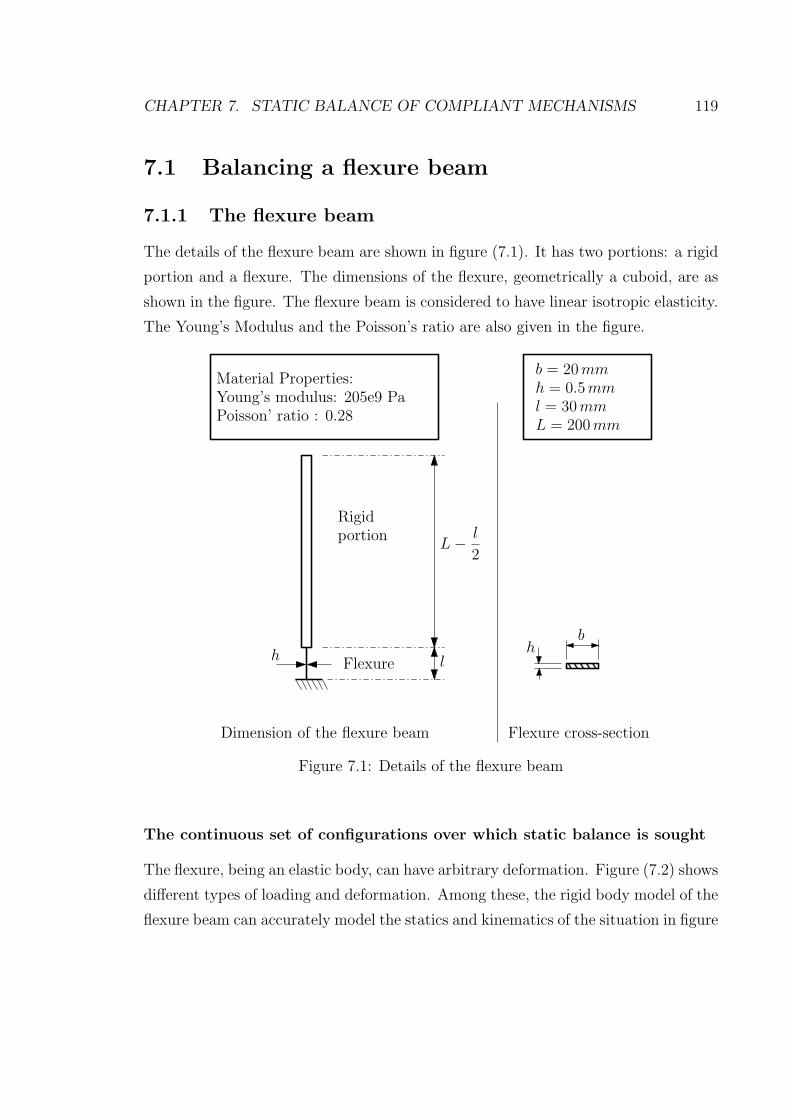
CHAPTER 7. STATIC BALANCE OF COMPLIANT MECHANISMS 119
7.1 Balancing a flexure beam
7.1.1 The flexure beam
The details of the flexure beam are shown in figure (7.1). It has two portions: a rigid
portion and a flexure. The dimensions of the flexure, geometrically a cuboid, are as
shown in the figure. The flexure beam is considered to have linear isotropic elasticity.
The Young’s Modulus and the Poisson’s ratio are also given in the figure.
l
L−
l
2
h
Material Properties:
Young’s modulus: 205e9 Pa
Poisson’ ratio : 0.28
Dimension of the flexure beam
Rigid
portion
Flexure
b = 20mm
h = 0.5mm
l = 30mm
L = 200mm
hb
Flexure cross-section
Figure 7.1: Details of the flexure beam
The continuous set of configurations over which static balance is sought
The flexure, being an elastic body, can have arbitrary deformation. Figure (7.2) shows
different types of loading and deformation. Among these, the rigid body model of the
flexure beam can accurately model the statics and kinematics of the situation in figure

CHAPTER 7. STATIC BALANCE OF COMPLIANT MECHANISMS 120
(7.2a). Here, the interest is to know what horizontal force at point P is necessary for
a range of horizontal displacements of point P . Our static balancing will focus on
considerably reducing this horizontal force over the range of horizontal displacements.
If this force is reduced to zero, it would become perfect static balancing but, as we
will see, it is not the case.
7.1.2 Rigid-body model for the flexure beam
When the flexure beam model [7] is applied to the flexure beam of figure (7.1) a
torsional spring-loaded lever results, as shown in figure (7.3). In this model, the
flexure is replaced by a revolute joint with a linear torsional spring at the joint. The
joint is usually placed at the centre of the flexure’s undeformed configuration. Further,
in the undeformed configuration, the moment exerted by the torsional spring is zero.
To obtain the spring constant, the flexure is modelled as an Euler-Bernoulli beam
(see [79]). An Euler-Bernoulli beam under pure moment will have a constant ratio
between the moment and the relative change in the tangent-angle of the end-points
of the beam. This ratio is evaluated for the flexure and it is taken as the torsional
spring constant. If E is the Young’s modulus of the flexure, I is the area moment of
inertia of the cross-section of the flexure and l is the length of the flexure, then the
ratio is given by
kt =EI
l(7.1)
The numerical values of the relevant quantities are tabulated in table 7.1.
Table 7.1: Relevant quantities to calculate the torsional stiffness of the spring
Numerical value for torsional spring
E Young’s modulus 205× 109[Pa]h Height of the flexure cross-sections 500× 10−6[m]b Width of the flexure cross-sections 2× 10⁻²[m]
I Area moment of inertia = bh3
122.083× 10⁻¹³[m4]
l Length of the flexures 3× 10⁻²[m]kt Torsional spring constant = EI
l1.424[N −m/rad]
L Lever arm length 0.2[m]
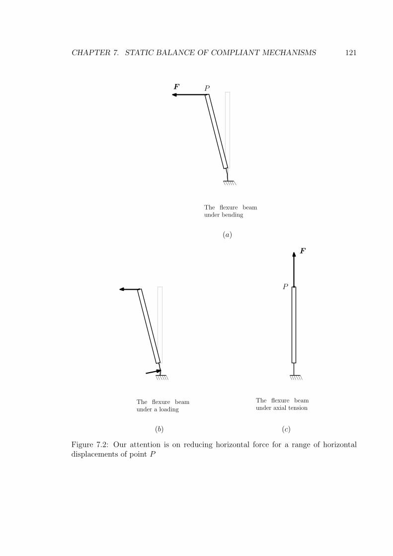
CHAPTER 7. STATIC BALANCE OF COMPLIANT MECHANISMS 121
The flexure beamunder bending
P
P
F
F
The flexure beamunder axial tension
The flexure beamunder a loading
(a)
(b) (c)
Figure 7.2: Our attention is on reducing horizontal force for a range of horizontaldisplacements of point P

CHAPTER 7. STATIC BALANCE OF COMPLIANT MECHANISMS 122
kt =EI
l
Case 1a Case 2a
Figure 7.3: Small-length-flexure model applied to the flexure beam
7.1.3 Approximation of torsional spring by zero-free-length
spring
We now approximate torsional springs by zero-free-length springs. This approxima-
tion is necessary since we know how to analytically static balance a linkage loaded by
zero-free-length springs but not a linkage with torsional springs.
Our eventual goal is to reduce horizontal force Fx over a range of horizontal dis-
placements ux of point P . So, a zero-free-length spring, shown in case 3a of figure (7.4)
can be considered to approximate the torsional spring of case 2a if the replacement of
the torsional spring by the zero-free-length spring does not significantly perturb Fx
vs. ux relation.
Case (2a) in figure (7.4) shows the lever with the torsional spring. This has to be
approximated by the lever loaded by a zero-free-length spring as shown in case 3a of
the same figure. The task now is to find the parameters of the zero-free-length spring
(spring constant and anchor points) so that Fx vs. ux curve for the two cases match
as closely as possible. Towards that, we find the zero-free-length spring parameters

CHAPTER 7. STATIC BALANCE OF COMPLIANT MECHANISMS 123
so that Fx and dFx
duxat ux = 0 match. With this, the two Fx vs. ux curves have the
same Taylor’s expansion upto the first order and we expect them to match atleast in
a range around ux = 0. The details of this are presented next.
Case 2a
PP
x
y
θ
x
y
θ
u
Positive rotational direction: anticlockwise
F
kt
k1 = ?
Case 3a
Figure 7.4: Approximation of the torsional spring by a zero-free-length spring
Fx vs. ux in the torsional spring-loaded lever (case 2a)
There may be ways to find Fx vs. ux relation that are simple in comparison to what
is presented next. However, for the sake of uniformity across the examples, we use
the principle of virtual work to get a balance equation form which Fx vs. ux relation
can be deduced. Let θ and δθ be the variables that parameterize the configuration
and its virtual change. The quantities related to the calculation of the virtual work
are as in table (7.2).
For static equilibrium at configuration θ, the net virtual work should be zero, i.e.,
−δθ (ktθ + FxL cos θ) = 0 (7.2)

CHAPTER 7. STATIC BALANCE OF COMPLIANT MECHANISMS 124
Table 7.2: Virtual work calculation for lever in case (2a)
Sl. no. description of quantities at the pivot at point P
1 generalized displacement θ u =
[−L sin θL cos θ
]
2 generalized force −ktθ F =
[Fx
0
]
3 generalized virtual displacement δθ −δθL
[cos θsin θ
]
4 virtual work −δθktθ −δθFxL cos θ
Equation (7.2) can be used to get the following expression for Fx as
Fx = −ktθ
L cos θ(7.3)
In table 7.2 we had already written ux as a function of θ, i.e.,
ux = −L sin θ (7.4)
Equations (7.3 and 7.4) give relation between Fx and ux in the parametric form. The
derivative or the slope of Fx vs. ux is given by
dFx
dux=
dFx
dθduxdθ
=
−ktL
(θ sin θ
cos2 θ+
1
cos θ
)
−L cos θ(7.5)
The reference configuration (corresponding to the undeformed configuration of the
flexure beam) corresponds to θ = 0. At θ = 0, Fx and dFx
duxare given as
Fx = 0 anddFx
dux=ktL2
(7.6)
Fx vs. ux in the lever loaded by zero-free-length spring (case 3a)
The lever loaded by zero-free-length spring is shown as case (3a) in figure (7.4). One
end of the spring is anchored at P and in the reference configuration (θ = 0) the

CHAPTER 7. STATIC BALANCE OF COMPLIANT MECHANISMS 125
spring is undeformed. The various quantities for calculating virtual work balance are
tabulated.
Table 7.3: Virtual work calculation and slope of Fx vs. ux
Sl. no. description of quantities at P (spring force) at P (force Fx)
1 generalized displacement u =
[−L sin θL cos θ
]
u =
[−L sin θL cos θ
]
2 generalized force k1L
[sin θ
(1− cos θ)
]
F =
[Fx
0
]
3 generalized virtual displacement −δθL
[cos θsin θ
]
−δθL
[cos θsin θ
]
4 virtual work −δθk1L2 sin θ −δθFxL cos θ
Virtual work balance:
−δθ(k1L2 sin θ + FxL cos θ) = 0 (7.7)
Fx and ux in parametric form
Fx = −k1L sin θ
cos θ(7.8)
ux = −L sin θ (7.9)
Slope of Fx vs. ux
dFx
dux=
dFx
dθduxdθ
=−k1L
(sin2 θcos2 θ
+ 1)
−L cos θ(7.10)
Fx and slope of Fx vs. ux at θ = 0
Fx = 0, anddFx
dux= k1 (7.11)
CHAPTER 7. STATIC BALANCE OF COMPLIANT MECHANISMS 126
The parameters of the zero-free-length spring in case 3a
The anchor points of the zero-free-length spring (see figure (7.4)) were chosen such
that in the reference configuration (θ = 0), Fx is zero. Thus, at θ = 0, Fx for case 2a
and case 3a trivially match (see equations (7.6) and (7.11)). The remaining unknown
parameter of the zero-free-length spring is its spring constant k1. This is found by
equatingdFx
duxat θ = 0 for the two cases. From equations (7.6) and (7.11), matching
of the slopes lead to the following expression for k1.
k1 =ktL2
(7.12)
Using the numerical values for kt and L, given in table 7.1, the numerical value for
k1 is 35.600 [N/m]. With this value of k1, we plot Fx vs. ux relation for both case 2a
and case 3a (from equations (7.3), (7.8) and (7.4)) for a range of 5cm displacement
of point P around its reference position, as shown in figure (7.5). The match is not
perfect since there are deviations, which grow towards either end. Nevertheless, for
the range of ux plotted, one can say, by examining the plot, that the deviations are
less than 5%.
7.1.4 Static balancing by addition of a zero-free-length spring
Case 3a of figure (7.4) is the simplest of revolute-jointed linkages and it has only
zero-free-length load. Hence, case 3a in figure (7.4) is apt for application of static
balancing method of Chapter 5. Case 3a of figure (7.4) is a lever. Hence, the loads
on it have to satisfy equations (5.10–5.11) for it to be in static balance. Towards
that, we add a zero-free-length spring of stiffness k2 = k1, as shown in figure (7.6).
It can be verified through table 7.4 that the original zero-free-length spring and the
additional zero-free-length spring together satisfy equations (5.10 – 5.11).
As a cross-check, one may also do virtual work analysis, similar to the way it is in
table 7.3. The virtual work calculation table is the same as that of table 7.3 except
for an additional column corresponding to the balancing spring, as shown in table
7.5.
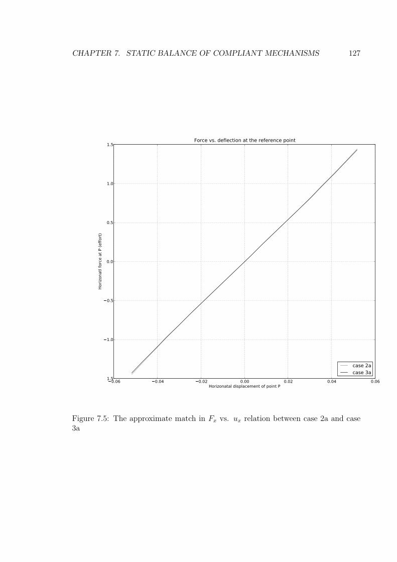
CHAPTER 7. STATIC BALANCE OF COMPLIANT MECHANISMS 127
�0.06 �0.04 �0.02 0.00 0.02 0.04 0.06Horizonatal displacement of point P
�1.5
�1.0
�0.5
0.0
0.5
1.0
1.5
Horiz
onat
l for
ce a
t P (e
ffort
)
Force vs. deflection at the reference point
case 2acase 3a
Figure 7.5: The approximate match in Fx vs. ux relation between case 2a and case3a

CHAPTER 7. STATIC BALANCE OF COMPLIANT MECHANISMS 128
Case (3b)
k1
k2 = k1
L
L
x0
y0x1
y1
Balancing spring
Figure 7.6: Static balance of the approximated zero-free-length spring-loaded leverby addition of a zero-free-length spring

CHAPTER 7. STATIC BALANCE OF COMPLIANT MECHANISMS 129
Table 7.4: Verification of equations (5.10–5.11) being satisfied
ki ai bi r ki(r − bi)Tai ki(r − bi)
TR(π2)ai
1stspring k1
[L0
] [0L
] [00
]
0 −k1L2
2ndspring k1
[L0
] [0−L
]
0 k1L2
Summation over two springs 0 0
Table 7.5: Verification of static balance through virtual work calculations
no. quantities Original spring balancing spring force Fx
1 displacement u =
[−L sin θL cos θ
]
u =
[−L sin θL cos θ
]
u =
[−L sin θL cos θ
]
2 force k1L
[sin θ
(1− cos θ)
]
k2L
[sin θ
(−1− cos θ)
]
F =
[Fx
0
]
3 virtual displ. −δθL
[cos θsin θ
]
−δθL
[cos θsin θ
]
−δθL
[cos θsin θ
]
4 virtual work −δθk1L2 sin θ +δθk2L
2 sin θ −δθFxL cos θ
Along the same lines as Section 7.1.3, we obtain
Virtual work balance:
−δθ((k1 − k2)L2 sin θ + FxL cos θ) = 0 (7.13)
Fx and its slope at θ = 0
Fx = −(k1 − k2)L sin θ
cos θ(7.14)
dFx
dux= k1 − k2, at θ = 0 (7.15)
From equation (7.14), it may be noted that when k1 = k2, the effort is zero for
any configuration.

CHAPTER 7. STATIC BALANCE OF COMPLIANT MECHANISMS 130
7.1.5 Balancing springs on the flexure beam
Case 3a approximates case 2a (see figure (7.4) and case 2a in turn approximates case
1a (see 7.3). Further, a perfectly statically balanced case 3b was obtained by adding
a balancing spring (see figure (7.6)). Case 1b, shown in figure (7.7), obtained by
adding the same balancing spring to the flexure of case 1a is expected to be at least
approximately statically balanced because of the approximation between case 1a and
case 3a. Figure (7.7), by the way, is a consolidation of all the cases.
To check the efficacy of balancing in case 1b, we performed finite element analysis
of the flexure beam using commercially available software COMSOL (www.comsol.com).
The flexure beam was modelled as a plane stress problem with geometric nonlinearity.
Point P was given a horizontal displacement constraint of ux (see figure (7.2)). Fx
was obtained as the reaction force of this constraint. By varying ux, Fx for a range
of values of ux was obtained. This analysis was carried out both with and without
balancing spring force. This data is plotted in figure (7.8).
It is important to note that prior to this, all the calculations to obtain the ap-
proximately balancing spring are analytical. The numerical simulation has been used
only to judge the effectiveness of this approximately balancing spring. In figure (7.8),
while the curve for f1b is not the ideal zero, it has reduced to less than 20% when
compared with unbalanced case 1a.
A way to improve the balance
Having carried out the numerical analysis to judge the effectiveness of the approximate
balance, we are in a position in to find deviation from perfect balance. In particular
we can know what deviations are there for Fx and its slope at the origin. Let us
call these quantities as c and m (these symbols are intended to allude to standard
equation of a straight line: y = mx + c). From the plot, there is no deviation in c
while the deviation in m is 5.4 [N/m]. Further, suppose that we can make changes to
parameters of the balancing spring, say to its stiffness k2. If we can find the sensitivity
of m with respect to k2, then we can make a first order correction to k2. While one
can find this sensitivity from finite element analysis, as a matter curiosity, we have

CHAPTER 7. STATIC BALANCE OF COMPLIANT MECHANISMS 131
(1a) (2a) (3a)
(1b) (2b) (3b)
P P P
PPP
Figure 7.7: All the cases related to the flexure and its approximation by the spring-loaded lever

CHAPTER 7. STATIC BALANCE OF COMPLIANT MECHANISMS 132
�0.06 �0.04 �0.02 0.00 0.02 0.04 0.06ux (m)
�3
�2
�1
0
1
2
3
Fx (N
)
f1a
f1b
f1c
Fx vs. ux at point P
Figure 7.8: Fx vs. ux relation obtained from finite element analysis of the flexurebeam
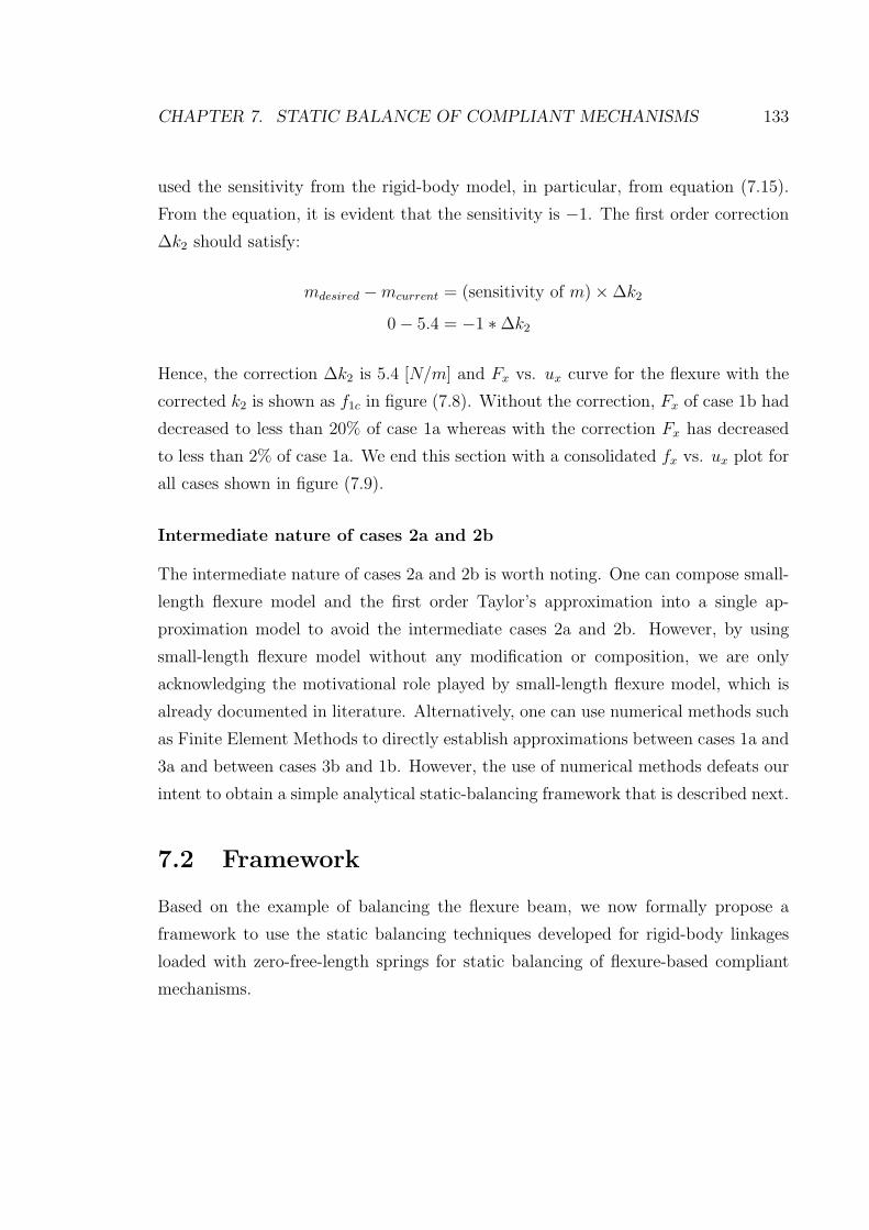
CHAPTER 7. STATIC BALANCE OF COMPLIANT MECHANISMS 133
used the sensitivity from the rigid-body model, in particular, from equation (7.15).
From the equation, it is evident that the sensitivity is −1. The first order correction
∆k2 should satisfy:
mdesired −mcurrent = (sensitivity of m)×∆k2
0− 5.4 = −1 ∗∆k2
Hence, the correction ∆k2 is 5.4 [N/m] and Fx vs. ux curve for the flexure with the
corrected k2 is shown as f1c in figure (7.8). Without the correction, Fx of case 1b had
decreased to less than 20% of case 1a whereas with the correction Fx has decreased
to less than 2% of case 1a. We end this section with a consolidated fx vs. ux plot for
all cases shown in figure (7.9).
Intermediate nature of cases 2a and 2b
The intermediate nature of cases 2a and 2b is worth noting. One can compose small-
length flexure model and the first order Taylor’s approximation into a single ap-
proximation model to avoid the intermediate cases 2a and 2b. However, by using
small-length flexure model without any modification or composition, we are only
acknowledging the motivational role played by small-length flexure model, which is
already documented in literature. Alternatively, one can use numerical methods such
as Finite Element Methods to directly establish approximations between cases 1a and
3a and between cases 3b and 1b. However, the use of numerical methods defeats our
intent to obtain a simple analytical static-balancing framework that is described next.
7.2 Framework
Based on the example of balancing the flexure beam, we now formally propose a
framework to use the static balancing techniques developed for rigid-body linkages
loaded with zero-free-length springs for static balancing of flexure-based compliant
mechanisms.
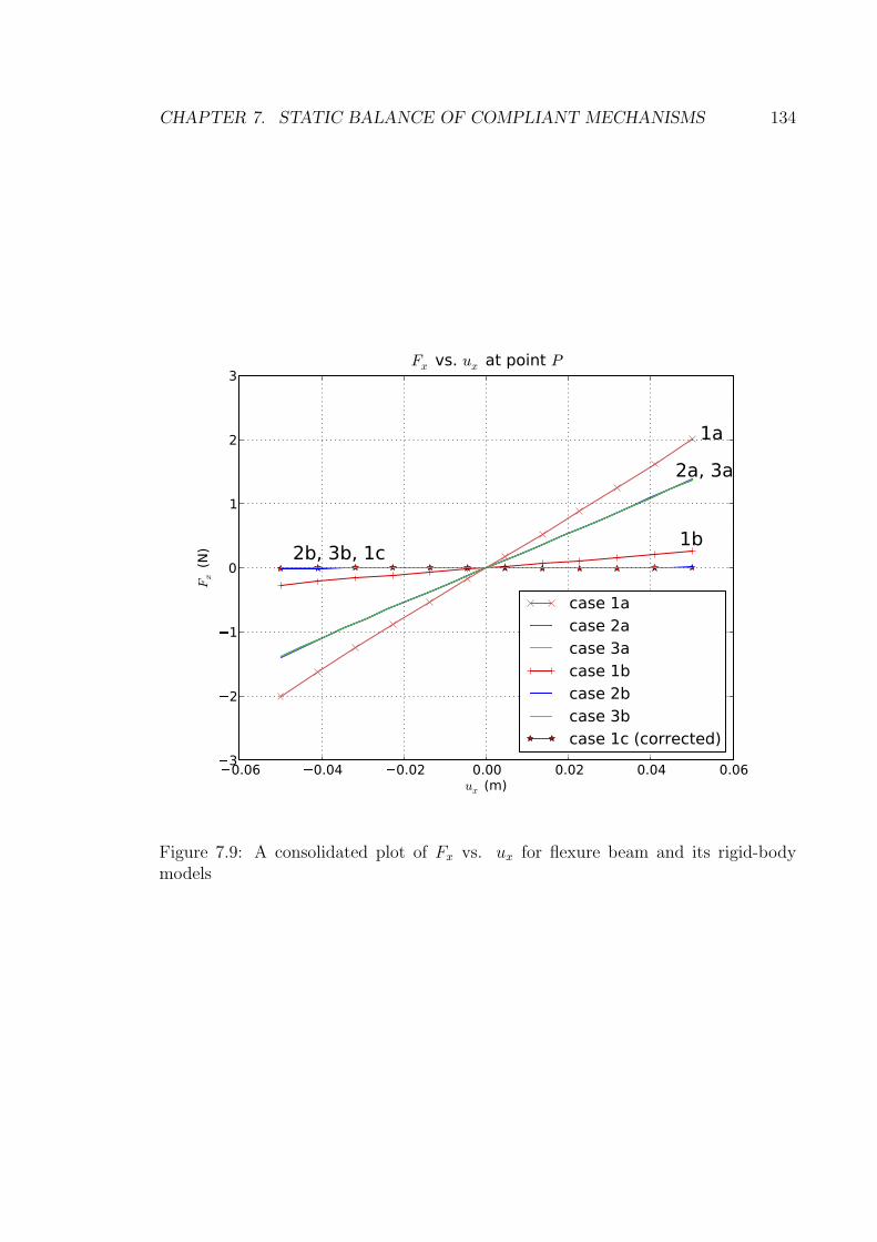
CHAPTER 7. STATIC BALANCE OF COMPLIANT MECHANISMS 134
�0.06 �0.04 �0.02 0.00 0.02 0.04 0.06ux (m)
�3
�2
�1
0
1
2
3
Fx (N
)
1a
2a, 3a
1b2b, 3b, 1c
Fx vs. ux at point P
case 1acase 2acase 3acase 1bcase 2bcase 3bcase 1c (corrected)
Figure 7.9: A consolidated plot of Fx vs. ux for flexure beam and its rigid-bodymodels

CHAPTER 7. STATIC BALANCE OF COMPLIANT MECHANISMS 135
Step 1: Apply small-length-flexure model to the given flexure-based compliant mecha-
nism to obtain a revolute-jointed rigid-body linkage loaded by torsional springs.
The given flexure-based compliant mechanism may be labelled as case 1a and
the linkage loaded by torsional springs as case 2a.
Step 2: Identification of an effort function. Identify a function whose closeness
to zero implies closeness of the system to static balance. The definition of the
function should preferably be such that it is convenient to compute it both in
flexure-based compliant mechanisms and rigid-link mechanisms.
Step 3: Torsional springs to zero-free-length springs. In this step, a new case,
labelled case 3a is formed where the torsional springs are substituted by zero-
free-length springs. The parameters of the zero-free-length springs should be
such that the effort function in case 2a and case 3a should have a close match.
In this thesis, to obtain the match, we ensure that there is a perfect match in
terms of the value of the function and the slope of the function at a reference
configuration. It is known that if two functions have the same value and slope
at a configuration then in a “small” range around the configuration, the two
functions “match closely”. This is the consequence of the match in the Taylor’s
expansion of the two functions upto the first order.
Step 4: Static balancing of the linkage with zero-free-length springs. Statically
balance the spring-loaded linkage of case 3a to obtain case 3b. In this thesis,
we propose the use of static balancing techniques of Chapter 5, where there
is no addition of auxiliary bodies. The previous step was necessary since, till
now, there are analytical static balancing principles only for rigid-body linkages
under zero-free-length spring loads and not under torsional spring loads.
Step 5: Whatever balancing zero-free-length springs were added in case 3b, add the
same springs to the compliant mechanism of case 1a to obtain case 1b. The
assumption here is that with cases 1a, 2a and 3a being approximately close
to each other, whatever additional load balances one case would balance other
cases also. Note that there are instances where this assumption may break

CHAPTER 7. STATIC BALANCE OF COMPLIANT MECHANISMS 136
down and so does the whole framework. Breakdown of this step is discussed in
Section 7.6.
A way to improve the static balance
In case 1b, the effort function and its slope are ideally expected to be zero. However,
due to approximations, generally there would be deviations. The deviations could be
found either by finite element analysis or by practical measurements. Based on the
sensitivity of the function value and its slope with respect to the balancing spring
parameters, one can do a first order correction to balancing spring parameters. This
generally brings effort function closer to zero. While the sensitivity should ideally be
evaluated for case 1b using finite element methods, in this thesis, out of curiosity, we
analytically obtain sensitivity based on case 3b. We label this corrected version of
case 1b as case 1c.
We now illustrate this framework on three more examples where the results are
encouraging.
7.3 Flexure-based compliant four-bar mechanism
7.3.1 Description of the mechanism
Figure (7.10) shows a flexure-based four-bar linkage. In the undeformed configuration,
all the flexures are vertical. All the flexures have the same geometrical dimensions
as well as elastic properties. Each flexure is a cuboid. The in-plane dimensions are
0.5 mm × 10 mm and the out-of-plane dimension is 40 mm. In the plane of motion
and in the undeformed configuration, the quadrilateral formed by the centers of the
flexures is a quadrilateral of sides a, b, c, and d with a diagonal of length l0, as shown
in figure (7.11). In the flexure at the vertex between sides c and d (see figure (7.11)),
the bottom-most point is labeled as P (see figure (7.10)). From the figure, it may
also be noted that P is at the centre of the interface between the flexure and the rigid
portion. This point is later used to define the effort function.

CHAPTER 7. STATIC BALANCE OF COMPLIANT MECHANISMS 137
Case 1a
P
Flexures
Flexures
Undeformed
configuration
Figure 7.10: A flexure-based four-bar linkage.
a = 150mm
b = 100mm
c = 130mm
d = 120mml0
l0 = 140mm
(drawing not to the scale)
Figure 7.11: The quadrilateral formed by the centers of the flexures

CHAPTER 7. STATIC BALANCE OF COMPLIANT MECHANISMS 138
7.3.2 Step 1
Application of small-length flexure model leads to torsional spring-loaded four-bar
linkage, as shown in figure (7.12). All the quantities required to calculate the spring
constant of the torsional spring are shown in the table of the same figure.
Case 2a
kt
kt
ktkt
P
Case 1a
P
E Young’s modulus 205e9[Pa]h Height of the flexure cross-sections 500e-6[m]b Width of the flexure cross-sections 4e-2[m]
I Area moment of inetria = bh3
124.167e-13[m4]
l Length of the flexures 1e-2[m]kt Torsional spring constant 8.5417[N-m/rad]
a
b
c
d
Figure 7.12: Approximation of the flexure-based four-bar linkage as a rigid-bodyfour-bar linkage with torsional springs.
7.3.3 Step 2 – The effort function
When point P is constrained to have a horizontal displacement of ux, there is a
corresponding horizontal constraint force Fx. The function Fx vs. ux over a range
[−0.025m,+0.025m] of ux is taken as the effort function.

CHAPTER 7. STATIC BALANCE OF COMPLIANT MECHANISMS 139
7.3.4 Step 3
We next propose to approximate the torsional springs of case 2a by two zero-free-
length springs as in figure (7.13). We further propose to fix the anchor points of the
springs at the coordinates shown in figure (7.13). We find the remaining parameters,
i.e., the spring constants, so that there is a close match in the effort function between
case 2a and case 3a. Towards that, at the reference configuration, the effort function
(Fx at ux = 0) and its slope (dFx/dux at ux = 0) for the two cases are analytically
found and tabulated in table 7.6. The details of this analytical calculation, which is
again based on virtual work balance as in Section 7.1, are presented as WXMAXIMA
(www.sourceforge.net) worksheet in Appendix F.1. To achieve a close match in effort
function between case 2a and case 3a, we equate Fx at ux = 0 and dFx/dux at ux = 0
between the two cases and solve the stiffness from the equations. The stiffness values
so obtained are shown in table 7.6.
Case 2a Case 3a
kt
kt kt
kt
Z2
1
Z1
1
P P
x0
y0
x1
y1
x2
y2
Spring a b klocal global stiffness
m m N/m
Z2
1
[
0.013−
13
300
] [
−0.050.06
]
k21
Z1
1
[
0.080
] [
0.25−0.05
]
k11
Figure 7.13: Approximation of torsional springs by zero-free-length springs
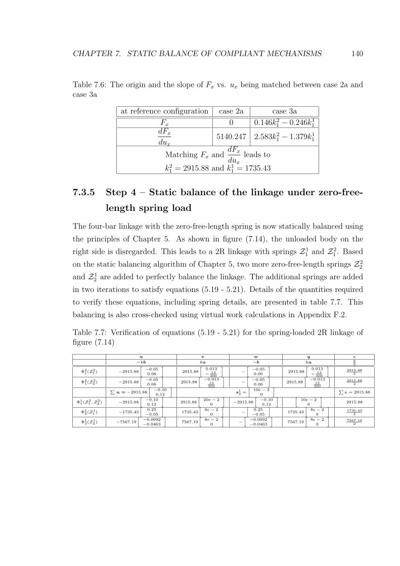
CHAPTER 7. STATIC BALANCE OF COMPLIANT MECHANISMS 140
Table 7.6: The origin and the slope of Fx vs. ux being matched between case 2a andcase 3a
at reference configuration case 2a case 3a
Fx 0 0.146k21 − 0.246k11dFx
dux5140.247 2.583k21 − 1.379k11
Matching Fx anddFx
duxleads to
k21 = 2915.88 and k11 = 1735.43
7.3.5 Step 4 – Static balance of the linkage under zero-free-
length spring load
The four-bar linkage with the zero-free-length spring is now statically balanced using
the principles of Chapter 5. As shown in figure (7.14), the unloaded body on the
right side is disregarded. This leads to a 2R linkage with springs Z11 and Z2
1 . Based
on the static balancing algorithm of Chapter 5, two more zero-free-length springs Z22
and Z12 are added to perfectly balance the linkage. The additional springs are added
in two iterations to satisfy equations (5.19 - 5.21). Details of the quantities required
to verify these equations, including spring details, are presented in table 7.7. This
balancing is also cross-checked using virtual work calculations in Appendix F.2.
Table 7.7: Verification of equations (5.19 - 5.21) for the spring-loaded 2R linkage offigure (7.14)
u v w q κ
−kb ka −b ka k
2
Φ2
1(Z2
1) −2915.88
[
−0.050.06
]
2915.88
[
0.013
−13
300
]
−
[
−0.050.06
]
2915.88
[
0.013
−13
300
]
2915.88
2
Φ2
1(Z2
2) −2915.88
[
−0.050.06
]
2915.88
[
−0.01313
300
]
−
[
−0.050.06
]
2915.88
[
−0.01313
300
]
2915.88
2
∑
u = −2915.88
[
−0.100.12
]
s12
=
[
10e − 20
]
∑
κ = 2915.88
Φ1
1(Z2
1,Z2
2) −2915.88
[
−0.100.12
]
2915.88
[
20e − 20
]
−2915.88
[
−0.100.12
] [
10e − 20
]
2915.88
Φ1
2(Z1
1) −1735.43
[
0.25−0.05
]
1735.43
[
8e − 20
]
−
[
0.25−0.05
]
1735.43
[
8e − 20
]
1735.43
2
Φ1
3(Z1
2) −7567.19
[
−0.0092−0.0463
]
7567.19
[
8e − 20
]
−
[
−0.0092−0.0463
]
7567.19
[
8e − 20
]
7567.19
2

CHAPTER 7. STATIC BALANCE OF COMPLIANT MECHANISMS 141
Case 3b
0
1
2
x0
y0
x1
y1
Z2
1
Z1
1
x2
y2
Z2
2
Z1
2
Spring a b klocal global
m m N/m
Z2
1
[
0.013−
13
300
] [
−0.050.06
]
2915.88
Z2
2
[
−0.01313
300
] [
−0.050.06
]
2915.88
Z1
1
[
0.080
] [
0.25−0.05
]
1735.43
Z1
2
[
0.080
] [
−0.0092−0.0463
]
7567.19
Figure 7.14: Static balancing by addition of zero-free-length springs

CHAPTER 7. STATIC BALANCE OF COMPLIANT MECHANISMS 142
7.3.6 Step 5 – Approximate static balance of flexure-based
four-bar linkage
Because of sucessive approximations from case 1a to case 2a and case 2a to case 3a, we
expect that whatever balances case 3a balances approximately case 1a too. Based on
this, the balancing springs Z22 and Z2
2 are added on to flexure-based four-bar linkage
as shown in figure (7.15–1b). Fx vs. ux plot for case 1a and case 1b, using finite
element simulation, is given in figure (7.16). From the plot, it may be seen that Fx
in case (1b) has reduced to less that 20% of case 1a.
(1a) (2a) (3a)
(1b) (2b) (3b)
P P P
Z2
1
Z1
1
Z2
1
Z1
1
Z2
2
Z1
2Z1
2
Z2
2Z2
2
Z1
2
Figure 7.15: A consolidated figure of all the cases
7.3.7 A way to improve the static balance of the flexure-
based four-bar linkage
However, from the plot of figure (7.16), for case 1b, at ux = 0 there is a deviation
for Fx and dFx/dux from their expected zero values. At ux = 0, let us call Fx and

CHAPTER 7. STATIC BALANCE OF COMPLIANT MECHANISMS 143
-100
-50
0
50
100
150
200
-0.02 -0.01 0 0.01 0.02
Fx
[N]
ux [m]
1a1b
Figure 7.16: Finite element simulation results for case 1a and case 1b
CHAPTER 7. STATIC BALANCE OF COMPLIANT MECHANISMS 144
dFx/dux as c and m and the deviations as δc and δm. We can make a first order
correction to these deviations by changing k22 and k12 as below:
[
−∆c
−∆m
]
=
∂c
∂k22
∂c
∂k12∂m
∂k22
∂m
∂k12
[
∆k22
∆k12
]
(7.16)
While the partial derivative in the matrix in equation (7.16) should ideally be found
by finite element method based sensitivity analysis, we analytically find them based
on the approximate rigid-body model of case 3b. The details of this calculation
are in Appendix F.3, where it turns out that the corrections are ∆k22 = 309.40 and
∆k12 = 510.51. One more finite element analysis of the flexure-based four-bar linkage
is carried out using the corrected k22 and k12 and Fx vs. ux relation turns out be as in
figure (7.17).
-100
-50
0
50
100
150
200
-0.02 -0.01 0 0.01 0.02
Fx
[N]
ux [m]
Case 1aCase 1b
Corrected
Figure 7.17: Fx vs. ux after first order correction to the stiffness of balancing springs

CHAPTER 7. STATIC BALANCE OF COMPLIANT MECHANISMS 145
We end this example with figure (7.18), which is a consolidated plot of all the
cases.
-100
0
100
200
300
400
-0.02 -0.01 0 0.01 0.02
Fx
[N]
ux [m]
1a1b
1c (corrected)2a2b3a3b
Figure 7.18: FX vs. ux plot for all the cases shown in figure (7.15)
7.4 Another flexure-based four-bar linkage
7.4.1 Description of the mechanism
This compliant mechanism is the same as in Section 7.3 except that the flexures are
longer as could be seen in case 1a of figure (7.19). Point P is also defined as in Section
7.3. Its location however is different because of the longer flexure.

CHAPTER 7. STATIC BALANCE OF COMPLIANT MECHANISMS 146
R R R
R R R
(1a) (2a) (3a)
(1b) (2b) (3b)
1
x1
y1
x0
y0
Z1
2
Z1
1
Figure 7.19: Consolidated figure containing all the cases

CHAPTER 7. STATIC BALANCE OF COMPLIANT MECHANISMS 147
Table 7.8: Details of the flexure and calculation of torsional spring constant
E Young’s modulus 205e9[Pa]h Height of the flexure cross-sections 500e-6[m]b Width of the flexure cross-sections 4e-2[m]
I Area moment of inetria = bh3
124.167e-13[m4]
l Length of the flexures 3e-2[m]kt Torsional spring constant 2.847[Nm/rad]
7.4.2 Step 1
Small-length-flexure model is applied on case 1a to obtain a torsional spring-loaded
rigid-body four-bar linkage (case 2a) as in figure (7.19). The details of the flexures
and the torsional spring constants are given table 7.8.
7.4.3 Step 2
The effort function is again Fx vs. ux where Fx is the horizontal reaction force
corresponding to a horizontal displacement constraint of ux on point P .
7.4.4 Step 3
We propose to approximate the torsional springs of case 2a by a single zero-free-length
spring as shown in case 3a of figure (7.19). Here again, the anchor point of the spring
is fixed and we assign such a spring constant so that there is a close match between
effort functions in case 2a and case 3a. The local coordinates of the anchor point on
body 1 (see case 3a in figure (7.19)) is [0.0632, 0.0301]Tm and the global coordinates
of the anchor point on the ground is [0, 0.07]Tm.
Table 7.9 shows, at ux = 0, Fx and dFx/dux. Fx is zero in both cases. dFx/dux
is a linear multiple of the stiffness in case 3a. By equating dFx/dux between the two
cases, we get the stiffness as shown in the same table. With this stiffness, the extent
of match between case 2a and case 3a could be seen in figure (7.20). The contents of
the table were arrived at analytically (using WXMAXIMA (www.sourceforge.net)) in
a manner similar to Section 7.3.
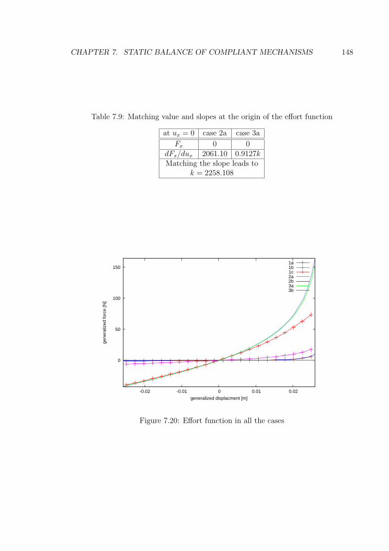
CHAPTER 7. STATIC BALANCE OF COMPLIANT MECHANISMS 148
Table 7.9: Matching value and slopes at the origin of the effort function
at ux = 0 case 2a case 3a
Fx 0 0dFx/dux 2061.10 0.9127kMatching the slope leads to
k = 2258.108
0
50
100
150
-0.02 -0.01 0 0.01 0.02
gene
raliz
ed fo
rce
[N]
generalized displacment [m]
1a1b1c2a2b3a3b
Figure 7.20: Effort function in all the cases

CHAPTER 7. STATIC BALANCE OF COMPLIANT MECHANISMS 149
Table 7.10: Details of the original spring and balancing spring
Spring a b klocal global stiffnessm m N/m
Z11
[0.06320.0301
] [0
0.07
]
2258.108
Z12
[0.06320.0301
]
−
[0
0.07
]
2258.108
7.4.5 Step 4
For the purpose of static balancing in case 3a, one only needs to consider the body
labelled as 1 (in figure (7.19)) along with the ground. With such a consideration,
this becomes a spring-loaded lever, similar to case 3a in Section 7.1. We balance the
spring Z11 with additional spring Z1
2 as shown in case 3b of figure (7.19). The details
of each of the springs is given in table 7.10. From the table, it may be verified that
the spring parameters satisfy the lever-balancing equations (5.10 – 5.11).
7.4.6 Step 5
The balancing spring of case 3b is incorporated into case 1a to obtain case 1b, as
shown in figure (7.19). The extent of balance in case 1b can be judged through the
plots in figure (7.20). Just by visual judgement, decrease in Fx to less than 30% of
case 1a can be noted.
7.4.7 First order correction
From the plot for case 1b in figure (7.20) it may be noted that at the origin, i.e.,
ux = 0, the slope of the plot deviates from the ideal zero-slope. The deviation
(calculated using finite element analysis data) is shown table 7.11. Using sensitivity
of the slope with respect to stiffness of the balancing springs (calculated from case 3a),
the correction is found in the same table. The effort function after this correction is
labelled as 1c in figure (7.20) and it may be noted that the effort function has indeed
become closer to zero.

CHAPTER 7. STATIC BALANCE OF COMPLIANT MECHANISMS 150
Table 7.11: First order correction of balancing spring parameters
Slope error Slope sensitivity w.r.t. k12 ∆k12N/m N/m
277.53 -0.913 304.055
7.4.8 Prototype
Based on this example, a prototype was made to demonstrate the reduction in effort of
a flexure-based compliant four-bar mechanism, as shown in figure (7.21). The image
in the figure is taken from the backside. Hence correlation between this and case
1b of figure (7.19) has to be done through a flipping transformation. The prototype
deviates from the example in one important respect. It uses normal springs having
finite free-length as balancing springs. In fact four balancing springs are used, which
are mostly in parallel, except for a little offset between anchor points. The balancing
springs were chosen such that the net force of all of them when extended between
anchor points is approximately same as what is exerted by the balancing spring of
case 1c of the example of this section. With further tuning in terms of varying the
number of active coils in springs, we could demonstrate a perceptible difference in the
effort to deflect the prototype mechanism. Almost all people who tried their hand on
this found the difference to be significant. Force measurements showed a reduction
in the effort to less than 25% over a range of 2 cm on either side of the reference
configuration.
What we want to suggest through this prototype is that the theoretical solution
serves as a guideline and one can deviate from the theoretical solution (in this case,
deviation was in free-length) with some compromise on static balance. This compro-
mise may be small enough to be acceptable in many practical situations.

CHAPTER 7. STATIC BALANCE OF COMPLIANT MECHANISMS 151
Figure 7.21: A prototype to demonstrate reduction in effort

CHAPTER 7. STATIC BALANCE OF COMPLIANT MECHANISMS 152
7.5 Flexure-based 2R compliant mechanism
7.5.1 Description of the compliant mechanism
The flexure-based compliant mechanism shown in case 1a of figure (7.22) is so con-
ceived that when small-length-flexure approximation is applied to it, it becomes a
2R linkage, as shown in case 2a of the same figure. Case 1a of figure (7.22) shows
points P , F1 and F2. F1 is the center of the first flexure and F2 is the center of the
second flexure. P is a point on the rigid portion that comes after the second flexure.
In the undeformed configuration, F1P is horizontal, F1P = 8 cm, PF2 = 6 cm, and
F1F2 = 10 cm.
(1a)
(1b)
(2a)
(2b)
(3a)
(3b)
P P
Z11
Z21F1
F2
Z22
Z12
Figure 7.22: A consolidation of all the cases
7.5.2 Step 1:
The small-length-flexure model is applied to case 1a to obtain torsional spring-loaded
rigid linkage as shown in figure (7.22–2a). The details of the flexures and the calcu-
lation of torsional spring constants from it are given in table 7.12.
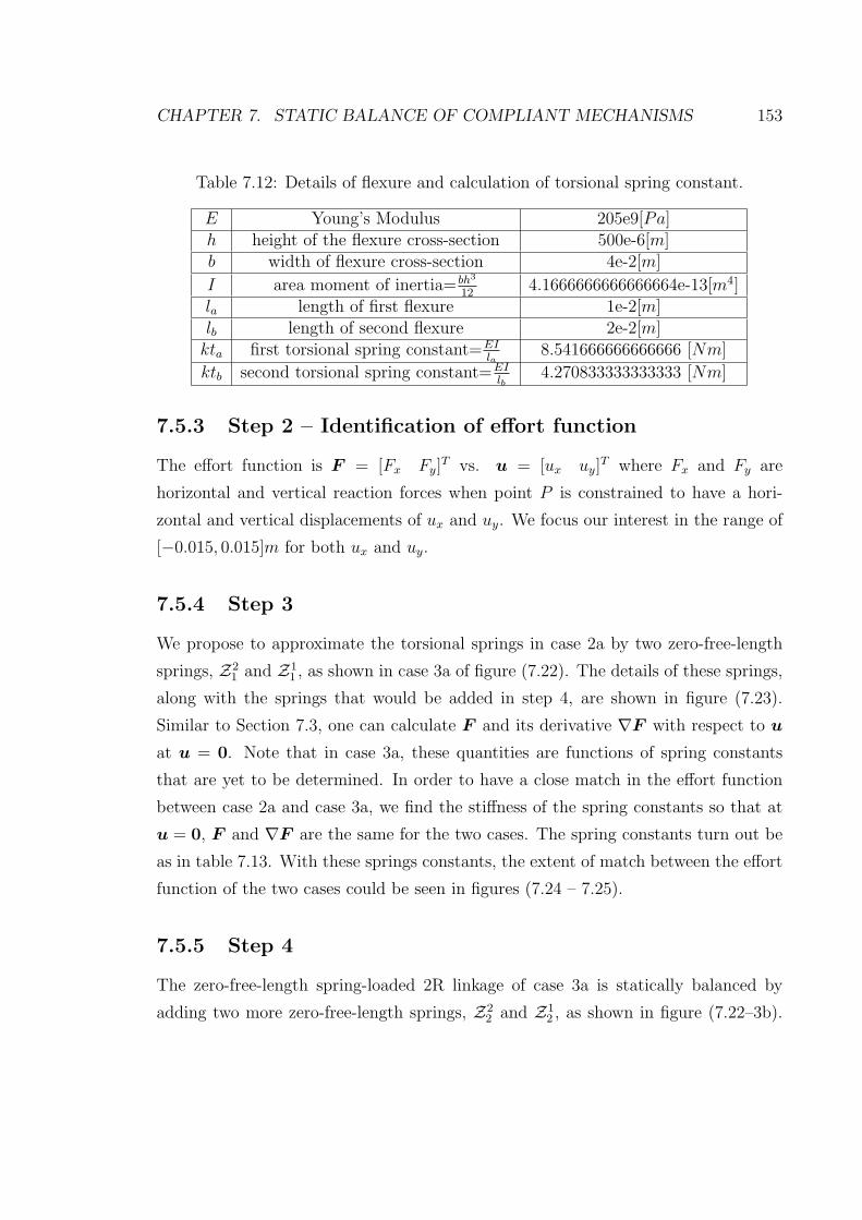
CHAPTER 7. STATIC BALANCE OF COMPLIANT MECHANISMS 153
Table 7.12: Details of flexure and calculation of torsional spring constant.
E Young’s Modulus 205e9[Pa]h height of the flexure cross-section 500e-6[m]b width of flexure cross-section 4e-2[m]
I area moment of inertia= bh3
124.1666666666666664e-13[m4]
la length of first flexure 1e-2[m]lb length of second flexure 2e-2[m]kta first torsional spring constant=EI
la8.541666666666666 [Nm]
ktb second torsional spring constant=EIlb
4.270833333333333 [Nm]
7.5.3 Step 2 – Identification of effort function
The effort function is F = [Fx Fy]T vs. u = [ux uy]
T where Fx and Fy are
horizontal and vertical reaction forces when point P is constrained to have a hori-
zontal and vertical displacements of ux and uy. We focus our interest in the range of
[−0.015, 0.015]m for both ux and uy.
7.5.4 Step 3
We propose to approximate the torsional springs in case 2a by two zero-free-length
springs, Z21 and Z1
1 , as shown in case 3a of figure (7.22). The details of these springs,
along with the springs that would be added in step 4, are shown in figure (7.23).
Similar to Section 7.3, one can calculate F and its derivative ∇F with respect to u
at u = 0. Note that in case 3a, these quantities are functions of spring constants
that are yet to be determined. In order to have a close match in the effort function
between case 2a and case 3a, we find the stiffness of the spring constants so that at
u = 0, F and ∇F are the same for the two cases. The spring constants turn out be
as in table 7.13. With these springs constants, the extent of match between the effort
function of the two cases could be seen in figures (7.24 – 7.25).
7.5.5 Step 4
The zero-free-length spring-loaded 2R linkage of case 3a is statically balanced by
adding two more zero-free-length springs, Z22 and Z1
2 , as shown in figure (7.22–3b).

CHAPTER 7. STATIC BALANCE OF COMPLIANT MECHANISMS 154
(3b)
x0
x1
x2
Z2
1
Z2
2
Z1
1Z1
2
spring a b klocal global stiffnessm m N/m
Z2
1
[
6e− 20
] [
8e− 20
]
1186.34
Z2
2
[
−6e− 20
] [
8e− 20
]
1186.34
coordinates of pivot of (1 to 2) revolute joint
s1
2=
[
10e− 20
]
Z1
1
[
8e− 20
] [
6.4e− 2−4.8e− 2
]
148.28
Z1
2
[
8e− 20
] [
−8e− 20.35e− 2
]
3151.22
Figure 7.23: Details of springs
Table 7.13: The value and the first derivative of F vs. u at u = 0
case 2a case 3a[N/m] [N/m]
F
[00
] [00
]
∇F
[1186.34 0
0 1334.63
] [k21 00 k21 + k11
]
k21 = 1186.34 and k11 = 148.29
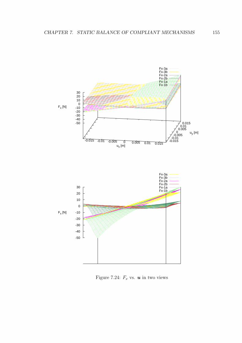
CHAPTER 7. STATIC BALANCE OF COMPLIANT MECHANISMS 155
Fx-3aFx-3bFx-2aFx-2bFx-1aFx-1b
-0.015 -0.01 -0.005 0 0.005 0.01 0.015ux [m]
-0.015-0.01
-0.005 0
0.005 0.01
0.015
uy [m]
-50-40-30-20-10
0 10 20 30
Fx [N]
Fx-3aFx-3bFx-2aFx-2bFx-1aFx-1b
-50
-40
-30
-20
-10
0
10
20
30
Fx [N]
Figure 7.24: Fx vs. u in two views

CHAPTER 7. STATIC BALANCE OF COMPLIANT MECHANISMS 156
Fy-3aFy-3bFy-2aFy-2bFy-1aFy-1b
-0.015-0.01
-0.005 0 0.005
0.01 0.015
ux [m]
-0.015 -0.01 -0.005 0 0.005 0.01 0.015
uy [m]
-30-20-10
0 10 20 30
Fy [N]
Fy-3aFy-3bFy-2aFy-2bFy-1aFy-1b
-30
-20
-10
0
10
20
30
Figure 7.25: Fy vs. u in two views

CHAPTER 7. STATIC BALANCE OF COMPLIANT MECHANISMS 157
Table 7.14: Verification of static balance of springs in case 3b
u v w q κ
−kb ka −b ka k2
Φ21(K2,1) −1186.34
[
8e − 20
]
1186.34
[
6e − 20
]
−
[
8e − 20
]
1186.34
[
6e − 20
]
1186.342
Φ21(K2,2) −1186.34
[
8e − 20
]
1186.34
[
−6e − 20
]
−
[
8e − 20
]
1186.34
[
−6e − 20
]
1186.342
∑
u = −1186.34
[
16e − 20
]
s12 =
[
10e − 20
]
∑
κ = 1186.34
Φ11(K2,1,K2,2) −1186.34
[
16e − 20
]
1186.34
[
20e − 20
]
−1186.34
[
16e − 20
] [
10e − 20
]
1186.34
Φ12(K1,1) −148.28
[
6.4e − 2−4.8e − 2
]
148.28
[
8e − 20
]
−
[
6.4e − 2−4.8e − 2
]
148.28
[
8e − 20
]
148.282
Φ13(K1,2) −3084.49
[
−8e − 20.35e − 2
]
3084.49
[
8e − 20
]
−
[
−8e − 20.23e − 2
]
3084.49
[
8e − 20
]
3084.492
The details of all the springs can be seen in figure (7.23). The static balance is done in
two iterations as per the balancing algorithm described in Section 5.4.2. To facilitate
verification of equations that are required to be satisfied by the algorithm of Section
5.4.2, the spring details are written in appropriate form in table 7.14.
7.5.6 Step 5
The balancing springs Z22 and Z1
2 present in case 3b are added on the compliant system
of case 1a to obtain case 1b as shown in figure (7.22). For the reasons discussed in
Section 7.2, we expect the effort function to be closer to zero in case 1b, in comparison
to case 1a. That it is indeed so can be seen in plots of figures (7.24 – 7.25) where
the plots for case 1a and 1b were obtained through a finite element analysis. In most
places, the effort has got reduced to less than 30% of that of case 1a.
7.6 Discussion
The proposed framework of Section 7.2 could fail if

CHAPTER 7. STATIC BALANCE OF COMPLIANT MECHANISMS 158
1. Rigid-body model does not very well approximate the actual flexure-based com-
pliant mechanism.
2. The range of configuration changes (in the examples, the range of ux or u that
was in focus) is very large around the undeformed configuration.
The second point is understandable because the rigid-body model of flexure-based
compliant mechanism are themselves valid over a finite but limited range around the
undeformed configuration. Secondly, the approximation between case 2 and 3 is based
on considering the Taylor’s series terms upto first order.
As far as the first point is considered, the deficiencies are the same as that of
the small-length flexure model. The model gets more accurate when the length of
the flexure becomes smaller. Sometimes, it may so happen that for a given flexure
length, the approximation between case 1a and case 2a/3a is acceptable but approx-
imation between case 1b and case 2b/3b is unacceptable. This happens because the
additional load that the flexures experiences due to balancing spring loads could be
high enough to make the flexure deform in way that is deviant from ideal circular
arc like deformation. We noticed this in the example of Section 7.3 when the flexure
length was made longer. In the example, let the length of all the flexures be increased
three times. Inspite of this change, cases 2 and 3 remain the same except that the
spring constants of all the springs change to one third of their values. Figure (7.26)
shows the effort function for cases 1a, 3a, 3b and 1b. It may be noted that the plot
for case 1b is quite different from what was noticed in previous examples. The effort
function of case 1b in some places around the origin is not even less that that of
case 1a. The way we reason is that in case 1a, without any balancing springs, the
deformation of the flexures resembled ideal arc like deformation, as shown in figure
(7.27–a). However, with the balancing springs, the load on the flexure, especially
the one at point O in figure (7.27–b), was high enough to have a non-ideal non-arc
like deformation. Because of this non-ideal deformation, coupled with longer length
of the flexure, the kinematics and statics of the flexure-based compliant mechanism
deviated largely from the rigid-body model of case 3b.

CHAPTER 7. STATIC BALANCE OF COMPLIANT MECHANISMS 159
0
50
100
150
-0.02 -0.01 0 0.01 0.02
Fx
[N]
ux [m]
Case 1aCase 1bCase 3aCase 3b
Figure 7.26: Plot of effort function when flexure length is increased three-fold
7.6.1 Static balancing of compliant mechanisms by individ-
ually balancing flexures
In flexure-based compliant systems, the elastic resistance to deformation arises due to
flexures. Hence, it is feasible to statically balance each of the flexures independently.
As an illustration, consider figure (7.28). The given compliant system is shown in
figure (7.28a) which is the same as that of the example in Section 7.5. In figure
(7.28c), the flexure between rigid portions A and B is statically balanced by adding
spring KA based on the principle that is the same as that used in figure (7.7), where
the flexure between the rigid-link and the ground is balanced by adding a spring.
Similarly, spring KB statically balances the flexure between the portion B and the
ground in figure (7.28c). The parameters of the spring KA are determined only by
the flexure between portions A and B and the spring reduces the effort only for the
relative motion between the rigid portions A and B. Similarly comments apply to
spring KB as well. This is what we mean when we say that each of the flexures are
balanced independently of each other. When each of the flexures in a flexure based
compliant system is balanced, the whole compliant system is balanced.
In the above scheme of balancing, the balancing springs were added only between

CHAPTER 7. STATIC BALANCE OF COMPLIANT MECHANISMS 160
O
(a)
(b)
Figure 7.27: Ideal circular arc-like and non-ideal deformation of flexures

CHAPTER 7. STATIC BALANCE OF COMPLIANT MECHANISMS 161
(a)
PF1
F2
(c)A
B
KA
KB
A
B
Figure 7.28: Static balancing of each of the flexures, independently of one another
successive rigid portions. However, such addition of springs only between successive
rigid links is infeasible for statically balancing gravity-loaded tree-structured rigid-
body linkages, as shown in appendix H.
7.6.2 Static balancing of compliant mechanisms using rigid-
body linkages
In this chapter, we developed a framework for approximately balancing compliant
mechanisms. The balancing elements used were springs, zero-free-length springs in
particular. Since, springs are also compliant elements, the eventual statically balanced
compliant mechanisms consist of only compliant elements. Note that it is not neces-
sary to have a pivot at points where springs anchor with the compliant mechanisms
since springs have negligible bending stiffness.
However, one can also statically balance compliant mechanisms using springs in
conjunction with rigid-body linkages, as shown in Appendix G. We have not empha-
sized this option since some of the advantages that compliant mechanisms have over
rigid-body linkages will be compromised in this option.
CHAPTER 7. STATIC BALANCE OF COMPLIANT MECHANISMS 162
Summary
• A way to make use of analytical rigid-body static balancing methods for ap-
proximate analytical static balancing of flexure-based compliant mechanism was
demonstrated through a simple flexure-beam.
• A framework for approximate analytical static balancing of flexure-based com-
pliant mechanisms was proposed.
• Three more examples based on the frame work have shown encouraging static
balance.
• That there is scope for further improvement through simple first order correction
was demonstrated.
• A prototype based on one of the examples was made and it did show perceptible
reduction in operating effort. The prototype also demonstrated that one can
pragmatically deviate from the theoretical solutions with a little compromise
on the extent of static balance.
• The situations where the proposed framework might fail was also discussed.
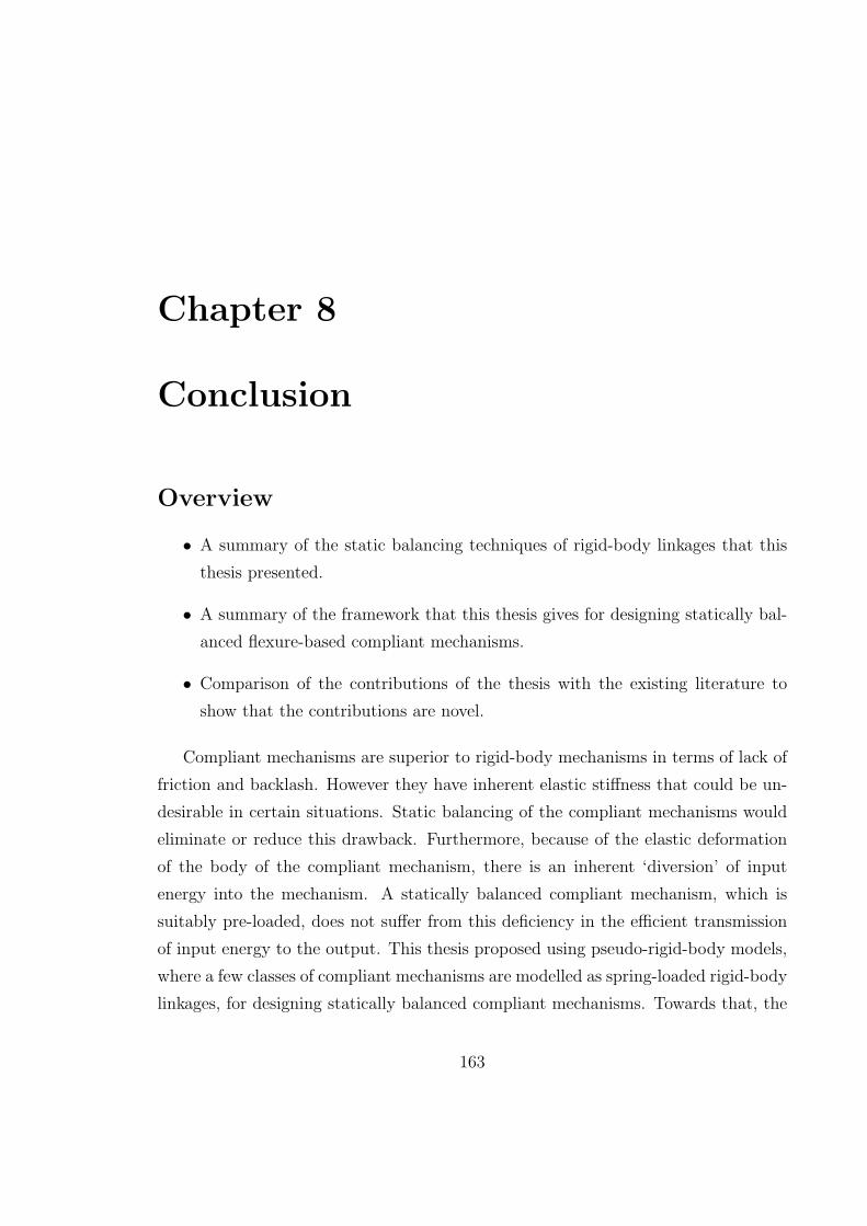
Chapter 8
Conclusion
Overview
• A summary of the static balancing techniques of rigid-body linkages that this
thesis presented.
• A summary of the framework that this thesis gives for designing statically bal-
anced flexure-based compliant mechanisms.
• Comparison of the contributions of the thesis with the existing literature to
show that the contributions are novel.
Compliant mechanisms are superior to rigid-body mechanisms in terms of lack of
friction and backlash. However they have inherent elastic stiffness that could be un-
desirable in certain situations. Static balancing of the compliant mechanisms would
eliminate or reduce this drawback. Furthermore, because of the elastic deformation
of the body of the compliant mechanism, there is an inherent ‘diversion’ of input
energy into the mechanism. A statically balanced compliant mechanism, which is
suitably pre-loaded, does not suffer from this deficiency in the efficient transmission
of input energy to the output. This thesis proposed using pseudo-rigid-body models,
where a few classes of compliant mechanisms are modelled as spring-loaded rigid-body
linkages, for designing statically balanced compliant mechanisms. Towards that, the
163

CHAPTER 8. CONCLUSION 164
contributions of the thesis are two fold: 1) the development of new analytical tech-
niques for statically balancing spring-loaded rigid-body linkages and 2) a framework
to use the techniques through small-length flexure model for designing statically bal-
anced compliant mechanisms.
8.1 A summary of new static balancing techniques
for spring and/or gravity-loaded rigid-body link-
ages
8.1.1 Static balancing of a four-bar linkage loaded by a spring
on its coupler link
Chapter 3 presented three techniques to statically balance a zero-free-length spring-
loaded four-bar linkage. The first technique requires two auxiliary bodies and one
balancing spring. The second technique requires two balancing springs without using
any auxiliary bodies. The third technique requires two auxiliary bodies and two
balancing springs. The second technique was demonstrated through a prototype.
8.1.2 Static balancing parameters and the cognates of a four-
bar linkage
Chapter 4 presented a unified parameterization for the triplet of the family of static
balancing solutions of the three cognates where the anchor points of the balancing
springs always form a triangle that is similar to the cognate triangle and the ratio of
spring constants of a set of corresponding balancing springs is a constant. This result
came out of a graphical solution that the chapter gave for a problem in geometry.
While the result of this chapter cannot be stated as a new static balancing method,
it helps in exploring various design possibilities as stated in the chapter.
CHAPTER 8. CONCLUSION 165
8.1.3 Static balancing without auxiliary bodies–planar case
Chapter 5, through systematic arguments based on making potential energy a con-
stant, gave an algorithm to statically balance any zero-free-length spring-loaded
and/or gravity-loaded revolute jointed rigid-body linkage. In the algorithm, the net
potential energy dependence on the rotational motion of the bodies making up the
linkage are recursively eliminated. The chapter gave several examples to illustrate
the algorithm.
8.1.4 Static balancing without auxiliary bodies–spatial case
Chapter 6 showed that the recursive static balancing algorithm of Chapter 5 also
works for spatial revolute and/or spherical jointed linkages under zero-free-length
spring and/or gravity loads. The chapter highlighted that revolute joints would re-
quire less stringent static balancing conditions. The chapter also gave an example to
illustrate the recursive algorithm in the spatial case.
8.2 A framework for designing statically balanced
compliant mechanisms
Chapter 7 provided a framework for using small-length-flexure model in conjunction
with the new static balancing methods of Chapter 5 for designing approximately
statically balanced compliant mechanisms. Flexure model of compliant mechanisms
gives rise to torsional spring-loaded rigid-body linkages whereas Chapter 5 deals with
static balance of zero-free-length (length extending) spring-loaded rigid-body link-
ages. Therefore, the framework proposed approximating torsional springs by zero-
free-length springs. Instead of using least squares approximation for this approxima-
tion, the framework proposed matching the value and the slope of the effort function
at a reference configuration as a way to approximate the two kinds of springs. This
allowed the framework to avoid numerical optimization. The chapter also presented

CHAPTER 8. CONCLUSION 166
four examples along with a prototype of one of the examples to illustrate the frame-
work.
8.3 The novelty of the contribution in the context
of the current literature
The contributions of the thesis covers the following areas of static balance.
1. Rigid linkages under gravity load
2. Rigid linkages under spring load
3. Compliant mechanism under their inherent elastic forces
Figure (8.1), a recapitulation of figure (8.1), pictorially depicts the current literature
as well our contribution (in grey boxes) under these broad areas. Our contribution
for static balancing of gravity-loaded rigid linkages falls within a category where the
methods (1) are perfect (in contrast to approximate methods), (2) add springs for
balancing, and (3) places no restriction on the degree-of-freedom of the linkages.
While there are methods in literature ([23], [27], and [29]) under the category, these
methods use auxiliary links in contrast to our method. Currently, under this category,
our contribution presented in chapters 5 and 6 is the only work that adds only springs
but not auxiliary links. Hence this is a novel contribution.
The literature is relatively sparse for the static balancing techniques of rigid link-
ages under spring loads. Apart from our contribution in this area that is presented
in Chapters 3, 5 and 6, the works in this area are [1], [4] and [65]. While [1] and [4]
deal with balancing zero-free-length spring loads by adding zero-free-length springs,
[65] stands apart as the one that balances, although approximately, torsional spring
loads by adding torsional springs. [4] and [1] give ways to statically balance a lever
and a four-bar linkage under zero-free-length spring loads. In the contribution stated
in Chapter 3, using the concepts not different from the one presented in [4], we give
more methods for the problem addressed in [1] (also see figure (1.9)). As far as the
methods that deal with a n-degree-of-freedom linkage under zero-free-length spring

CHAPTER 8. CONCLUSION 167
Rigid linkages
under
gravity load
By
addition
of mass
Rigid linkages
under
spring load
Compliant
mechanism
By
addition
of springs
Approximate
balancing
and
cam using
methods
Perfect
balancing
methods
Gopalswamy et al. (1992)
Agrawal & Agrawal (2005)
Ulrich & Kumar (1991)
Koser (2009)
For
specific
linkages
For
‘n’ - dof
linkages
LaCoste (1934)
Shin & Streit (1991)
Walsh et al. (1991)
Herder (2001)
Lin et al. (2010)
Using
auxiliary
bodies
Without
auxiliary
bodies
Streit & Shin (1993)
Agrawal & Fattah (2004)For planar revolutejointed and spatialrevolute and/orspherical jointedlinkages
Torsion
load
balanced
by
torsion
loads
Extension
spring
balanced
by
extension
springs
Approximate
methods
Perfect
methods
Radaelli et al. (2011)
For
specific
linkages
For
‘n’ -dof
linkages
Basic spring forcebalancer (Herder(2001))
Herder (1998)
Without
auxiliary
bodies
For planar revolutejointed and spatialrevolute and/orspherical jointedlinkages
Deepak & Ananthasuresh (2012)
Limiting case
By
addition
of springs
Other
strategies
Extension ofDeepak & Anan-thasuresh (2012)to compliantmechanisms usingpseudo-rigid bodymodel
Topology optimiza-tion (see De Lange etal. (2008))
Building block ap-proach (see Hoet-mer, et al. (2010))
Extension ofRadaelli et al.(2011) to compliantmechanisms as seenin Rosenberg et al(2011)
Original or novel contribu-
tions of this thesisdof: degree of freedom
Figure 8.1: The current literature and our contributions

CHAPTER 8. CONCLUSION 168
loads, we haven’t found any literature. Hence, our contribution stated in Chapters 5
and 6 for a n-degree-of-freedom linkage is new.
A few reported works in the literature on static balance of compliant mechanisms
are listed in figure (8.1). As far as the ones that rely on spring-loaded rigid linkage
balancing techniques, using flexure model as the interface between rigid mechanisms
and compliant mechanisms, there is a work by Rosenberg et al. [73]. However,
they rely on numerical optimization and their method is not completely analytical.
This should signify that our contribution in Chapter 7 is distinct from the existing
literature. Furthermore, that rigid-link balancing techniques could be used for flexure-
based compliant mechanisms was first enunciated in our work [8] (reported in 2009).
8.4 Future work
We now briefly outline the prospects of continuing the work from the thesis.
• In this thesis, though the main algorithm developed in Chapter 5 was for tree-
structured linkages, we showed how to extend it to closed loop linkages. The
concept behind this extension was straightforward and the design obtained
was conservative. An investigation on overcoming this conservative design is
a prospect for future work. The investigation could be based on the work of
Shieh and Chen [41] which exploits closed loop equations.
• Addition of springs during static balancing leads to increase in internal stresses
of the material making up the linkage. This is true in our compliant mechanism
methodology as well. It is useful to investigate ways of reducing this internal
stress without sacrificing the static balance.
Summary
• A summary of previous chapters.
• A comparison with the existing literature to show the distinctness of the con-
tributions of this thesis from the existing literature.

Appendix A
Proofs on finding the focal pivot
A.1 If Ia,b and Ic,a circles are coincident, then the
given lines a, b and c has to be concurrent
In the following proof, a, b, c, Ia,b and Ic,a refer to their original position before
rotation by β. Figure (A.1) shows Ia,b and Ic,a circles that are coincident. Also shown
are lines a and b and their intersection point Ia,b. The point Ic,a lie on this common
circles, since the circles is its locus. By the definition of Ic,a as the intersection of c
and a, it should also line on line a. Hence Ic,a should lie on the intersection of the
circle with the line a.
Since Ic,a and Ia,b circles, by definition pass through A and line a also by definition
pass through A, A is always an intersection point between the line and the circle. The
following types of intersection between the circle and line a are possible:
1. When Ia,b is distinct from A, the line a intersects the circle at two distinct points
:A and Ia,b, as shown in figure (A.1).
2. When Ia,b coincides with A, the line a has to be tangent to the circle at A. (see
the theorem in appendix (B)).
In the first possibility, Ic,a has be either at Ia,b or at A. If it is at A, then line a
has to be tangent to the circle (see the theorem in appendix (B)), which contradicts
169
APPENDIX A. PROOFS ON FINDING THE FOCAL PIVOT 170
b
AC
Ba Ia,b
Coincident Ia,b and Ic,a circles
Before rotation (at β = 0)
Figure A.1: Ia,b and Ic,a circles are coincident
the earlier observation that line a intersects the circle at two distinct points. Hence
it Ic,a cannot be at A and by elimination, has to be at Ic,a. This implies that Ia,b and
Ic,a coincide, which further imply that a, b, and c are concurrent.
In the second possibility, since A is the only intersection between line a and locus of
Ic,a, Ic,a has be at A. Thus, here also both Ia,b and Ic,a coincide implying concurrence
of lines a, b and c.
Hence, if Ia,b and Ic,a circles are coincident, then the given lines a, b and c has to
be concurrent.
A.2 When M and A are distinct, M is the fo-
cal pivot. (Refer to section (4.2.4 and figure
(4.11).)
Let rotation angle β be such that point Ia,b is at A, so that by the theorem in appendix
B, line b aligns along the segment AB and line a becomes tangent to Ia,b circle. If
for the same β, point Ic,a is also at A, then by the theorem in appendix B, line a
becomes tangent to Ic,a circle. This implies that line a is a common tangent to both
Ia,b and Ic,a circles at the A, which is one of the two distinct points of intersection
of the two circles. This contradicts the fact that for two circles intersecting at two
distinct points, there cannot be common tangent at the point of intersection. Hence

APPENDIX A. PROOFS ON FINDING THE FOCAL PIVOT 171
AC
B
ab
M ∼= Ia,b
δ
δ
Figure A.2: Ia,b is at M
there is no β, for which both Ia,b and Ic,a are at A. Therefore A is not a focal pivot.
Let rotation angle β be such that Ia,b is at M as shown in figure (A.2). It may
further be seen that not only circle Ia,b but even line a intersects the Ic,a circle at two
distinct points: A and M . Since point Ic,a has to lie on both its locus Ic,a circle and
on line a (by definition), it should be at one of the intersection points (A or M) of
the circle and the line.
If point Ic,a is at A, then by the theorem in appendix B, line c aligns along CA
and line a becomes tangent to Ic,a circle at A. This contradicts the earlier noted fact
that line a intersects at two distinct points. Hence, point Ic,a cannot be at A and by
elimination of choices, it has to be at M Thus for the angle of rotation β, Ic,a as well
as Ia,b lies on M , implying that M is a focal pivot.
Appendix B
An elementary theorem of
geometry
A chord of a circle subtends the same angle at any point on the circumference of the
circle. The converse of the theorem is as follows: If two non-parallel lines passing
through two ends of a line segment are rotated equally about the respective end-
points of the segment, then the intersection point of the two lines traces a circle. The
circle has the line segment as its chord. During rotation, when the intersection point
reaches one end of the chord, one of the lines will align along the chord while the
other becomes tangent to the circle.
172
Appendix C
Perfect static balance and
positive-free-length springs
This is an appendix to section 5.2. Here the difficulty in achieving perfect static
balance of a lever by using normally available positive free-length springs is discussed.
The dTd term in the potential energy expression of a spring given in equation
(5.5) was seen to be a linear combination of sin θ, cos θ and 1 when expanded as in
equation (5.6). Hence, by writing dTd as α sin θ + β cos θ + γ, the potential energy
expression of the spring becomes:
(k
2(α sin θ + β cos θ + γ)− kl0
√
(α sin θ + β cos θ + γ) +k
2l20
)
(C.1)
The first term in equation (C.1) is the zero-free-length part and the second term is
the free-length part. If the free-length is positive, i.e., l0 > 0, then the free-length
part is negative. The free-length part of the spring is non-constant (i.e., k 6= 0 and
not both α and β is zero) except for trivial situations where spring constant is zero
or the spring is attached to the pivot of the lever. When there are several but finite
positive-free-length and non-trivial springs, the net contribution of the free-length
part is negative, and it is also not known have the possibility of being a constant,
unlike the zero-free-length part. Furthermore, the free-length part is also not known
173

APPENDIX C. NORMAL SPRINGS 174
to be in the function space spanned by sin θ and cos θ. Hence, the possibility of free-
length part cancelling (modulo a constant) with zero-free-length part is also ruled
out. Thus, with several positive-free-length springs, there is no way the net potential
energy could become a constant.

Appendix D
Constraints can be satisfied, if not
as it is, by addition of extra
zero-free-length spring loads
D.1 Satisfying constraints (5.12), (5.13) and (5.14)
This appendix demonstrates how by adding extra zero-free-length spring loads con-
straints (5.12), (5.13) and (5.14) can be satisfied. To differentiate between original
loads and balancing loads, let ns,o and ns,b respectively represent the number of orig-
inal and balancing zero-free-length spring loads with ns,o + ns,b = ns. Also, let the
spring loads be indexed such that the first ns,o loads are original loads with the re-
maining being balancing loads. Similar meaning applies for nc,o and nc,b.
Case 1: Original loads violate the constraint (5.14), and balancing loads are only
zero-free-length springs.
Let us try to satisfy all the constraints by adding a single zero-free-length spring.
As per the notation, this spring gets the index i = ns,o+1. The constraint (5.14)
can be written as follows:
kns,o+1ans,o+1 = −
ns,o∑
i=1
kiai (D.1)
175
APPENDIX D. SATISFYING CONSTRAINTS 176
where the known quantities related to original loads are on the right hand side.
Equation (D.1) gives the unique solution of kiai for i = ns,o+1 to the constraint
(5.14). Furthermore, the constraints (5.12) and (5.13) can be rewritten as
([
kiax,i kiay,i
−kiay,i kiax,i
][
bx,i
by,i
])
i=ns,o+1
=
−nc∑
i=1
((fyipy,i + fx,ipx,i))−ns,o∑
i=1
(ki(ay,iby,i + ax,ibx,i))
+nc∑
i=1
((fx,ipy,i − fy,ipx,i))−ns,o∑
i=1
(ki(ax,iby,i − ay,ibx,i))
(D.2)
The 2× 2 matrix on the left hand side of the equations is known since kiai for
i = ns,o + 1 is already solved in equation (D.1). Furthermore, the matrix is
non-singular since the right hand side of (D.1) that is the same as kns,o+1ans,o+1
is non-zero as per the description this case. We take[
bx,i by,i
]T
for i = ns,o+1
as the inverse of the 2 × 2 matrix times the right hand side of the equation
(D.2) so that the constraints (5.12) and (5.13) can also be satisfied. Thus, the-
oretically, with a single additional zero-free-length spring, all three constraints
(5.12), (5.13) and (5.14) can be satisfied.
Case 2 Original loads satisfy (5.14), but violate atleast one of the constraints (5.12)
and (5.13). Balancing loads are only zero-free-length springs.
If we proceed along the same lines as the previous case, then in equation (D.2)
the 2×2 matrix on the left hand side becomes singular zero-matrix whereas the
right hand side is non-zero by the description of the case. Thus, in this case,
with a single balancing zero-free-length spring, it is not possible to satisfy the
related constraint. However, it may be verified that by adding two balancing
springs, all the constraints can be satisfied.
The cases 1 and 2 cover all possible types of constraint violation. Hence we assert
that if the constraints are not satisfied as it is, then by adding a minimum of one zero-
free-length spring in case (1) (the component related to original loads in constraint
(5.14) is non-zero) and two zero-free-length spring in case (2) (the component related

APPENDIX D. SATISFYING CONSTRAINTS 177
to original loads in constraint (5.14) is zero), the constraints can be satisfied.
D.2 Satisfying constraints (5.19), (5.20) and (5.21)
In appendix B1, if the constraints (5.12), (5.13) and (5.14) are respectively substituted
by constraints (5.19), (5.20) and (5.21), there is going to be no change except for the
right hand side of equation (D.1), which takes the form−no∑
i=1
vi and the right hand side
of equation (D.2), which takes the form−[n∑
i=1
(qy,iwy,i + qx,iwx,i)n∑
i=1
(qx,iwy,i − qy,iwx,i)]T .
There is no change in the left hand side since here also, the additional loads are zero-
free-length springs. Hence, analogous to the conclusion of appendix B1, we conclude
that if the constraints (5.19), (5.20) and (5.21) are not satisfied as it is, then by
addition of a minimum of one zero-free-length spring in case the constraint (5.21) is
originally violated and a minimum of two zero-free-length springs in case the con-
straint (5.21) is not originally violated, the three constraints can be satisfied.
Appendix E
Solving constraints on spatial
orientation independence for the
parameters of additional
zero-free-length springs
This is an appendix to proof of proposition 3. Let the number of zero-free-length
springs, na, be 3. With this equations (6.7) and (6.8) can be split as
[
vnf+1 vnf+2 vnf+3
] [
1 1 1]T
= −
nf∑
i=1
vi (E.1)
[
qnf+1 qnf+2 qnf+3
] [
wnf+1 wnf+2 wnf+3
]T
= −[
q1 · · · qnf
] [
w1 · · · wnf
]T(E.2)
The left hand side of equation are due zero-free-length springs and using relation
(5.17), the parameters ui, wi and qi on the left hand side can be written in terms of
(ki,ai, bi), ki > 0 and i = 1 · · · 3 as
[
k1a1 k2a2 k3a3
] [
1 1 1]T
= −
nf∑
i=1
vi (E.3)
178

APPENDIX E. SOLVING BALANCING CONSTRAINTS – SPATIAL CASE 179
−[
k1a1 k2a2 k3a3
] [
b1 b2 b3
]T
= −[
q1 · · · qnf
] [
w1 · · · wnf
]T(E.4)
Solution to equations (E.3) and (E.4)
Suppose thatnf∑
i=1
vi 6= 0. In the three dimensional space, one can always find a plane
such thatnf∑
i=1
vi 6= 0 is not along the plane. Let m1 and m2 be two two linearly
independent vectors along such a plane. As a result, the matrix[
m1 m2
(
−m1 −m2 −nf∑
i=1
vi
)]
is a full-rank invertible 3 × 3 matrix and also a
solution to the matrix[
k1a1 k2a2 k3a3
]
in equation (E.3). With this as the solution
for[
k1a1 k2a2 k3a3
]
, the matrix[
b1 b2 b3
]T
can be solved by pre multiplying
equation (E.4) with the inverse of[
k1a1 k2a2 k3a3
]
. With this, one has a solution
for k1a1, k2a2, k3a3, b1, b2, and b3. By choosing a convenient positive value for k1,
k2 and k3, one can obtain a1, a2 and a3 as well. Thus, whennf∑
i=1
vi 6= 0 there exist a
non-unique solution for {ki, ai, bi}, i = 1 · · · 3 in equations (6.7) and (6.8).
General case including the possibility ofnf∑
i=1
vi = 0
Whennf∑
i=1
vi = 0 four zero-free-length spring are sufficient to satisfy (6.7) and (6.8),
as shown next. Just as equations (6.7) and (6.8) took the form of equations (E.3)
and (E.4) for three springs, the equations take the following form for four spring.
[
k1a1 k2a2 k3a3 k4a4
] [
1 1 1 1]T
= −
nf∑
i=1
vi (E.5)
−[
k1a1 k2a2 k3a3 k4a4
] [
b1 b2 b3 b4
]T
= −[
q1 · · · qnf
] [
w1 · · · wnf
]T(E.6)

APPENDIX E. SOLVING BALANCING CONSTRAINTS – SPATIAL CASE 180
Let m1, m2 and m3 be any linearly independent vectors in three dimensional space.
The matrix
[
m1 m2 m3
(
−m1 −m2 −m3 −nf∑
i=1
vi
)]
is a solution for[
k1a1 k2a2 k3a3 k4a4
]
in equation (E.5) and at the same time is of full-rank.
With[
k1a1 k2a2 k3a3 k4a4
]
being full rank, there exists solution, though non-
unique, for[
b1 b2 b3 b4
]T
in equation (E.6) not matter what the right hand side
of the equation is. Now we have a solution for {kiai, bi}, i = 1 · · · 4. By choosing a
convenient positive value for ki, one can solve for ai from the known kiai. Thus, there
is always a solution for spring parameters {ki, ai, bi}, i = 1 · · · 4 so that equation
(6.7) and (6.8) are satisfied.
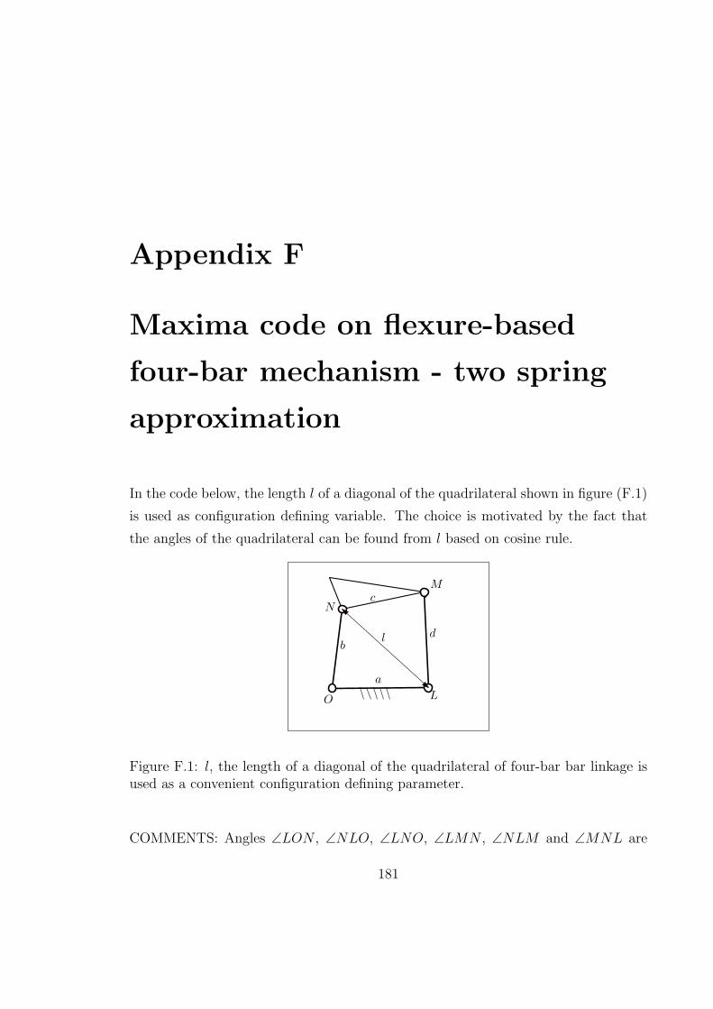
Appendix F
Maxima code on flexure-based
four-bar mechanism - two spring
approximation
In the code below, the length l of a diagonal of the quadrilateral shown in figure (F.1)
is used as configuration defining variable. The choice is motivated by the fact that
the angles of the quadrilateral can be found from l based on cosine rule.
a
b
c
d
O L
M
N
l
Figure F.1: l, the length of a diagonal of the quadrilateral of four-bar bar linkage isused as a convenient configuration defining parameter.
COMMENTS: Angles ∠LON , ∠NLO, ∠LNO, ∠LMN , ∠NLM and ∠MNL are
181

APPENDIX F. VIRTUAL WORK CALCULATIONS 182
written below as functions of l.
(%i1) theta_l_ab : acos( (a^2 + b^2 - l^2)/(2*a*b) );
(%o1) acos
(−l2 + b2 + a2
2 a b
)
(%i2) theta_b : acos( (a^2 + l^2 - b^2)/(2*a*l) );
(%o2) acos
(l2 − b2 + a2
2 a l
)
(%i3) theta_a : acos( (l^2 + b^2 -a^2)/(2*b*l) );
(%o3) acos
(l2 + b2 − a2
2 b l
)
(%i4) theta_l_cd : acos( (c^2 + d^2 - l^2)/(2*c*d) );
(%o4) acos
(−l2 + d2 + c2
2 c d
)
(%i5) theta_c : acos( (l^2 + d^2 - c^2)/(2*l*d) );
(%o5) acos
(l2 + d2 − c2
2 d l
)
(%i6) theta_d : acos( (l^2 + c^2 - d^2)/(2*l*c) );
(%o6) acos
(l2 − d2 + c2
2 c l
)
COMMENTS: The angles and their derivatives with respect to l of the four corners
of the quadrilateral of pivots shown in figure (F.1).
(%i7) psi_ab : theta_l_ab;

APPENDIX F. VIRTUAL WORK CALCULATIONS 183
(%o7) acos
(−l2 + b2 + a2
2 a b
)
(%i8) d_psi_ab : diff(psi_ab, l);
(%o8)l
a b
√
1− (−l2+b2+a2)2
4 a2 b2
(%i9) psi_bc : theta_a + theta_d;
(%o9) acos
(l2 − d2 + c2
2 c l
)
+ acos
(l2 + b2 − a2
2 b l
)
(%i10) d_psi_bc : diff(psi_bc,l);
(%o10) −1c− l2−d2+c2
2 c l2√
1− (l2−d2+c2)2
4 c2 l2
−1b− l2+b2−a2
2 b l2√
1− (l2+b2−a2)2
4 b2 l2
(%i11) psi_cd : theta_l_cd;
(%o11) acos
(−l2 + d2 + c2
2 c d
)
(%i12) d_psi_cd : diff(psi_cd, l);
(%o12)l
c d
√
1− (−l2+d2+c2)2
4 c2 d2
(%i13) psi_da : theta_c + theta_b;
(%o13) acos
(l2 + d2 − c2
2 d l
)
+ acos
(l2 − b2 + a2
2 a l
)
(%i14) d_psi_da : diff(psi_da, l);
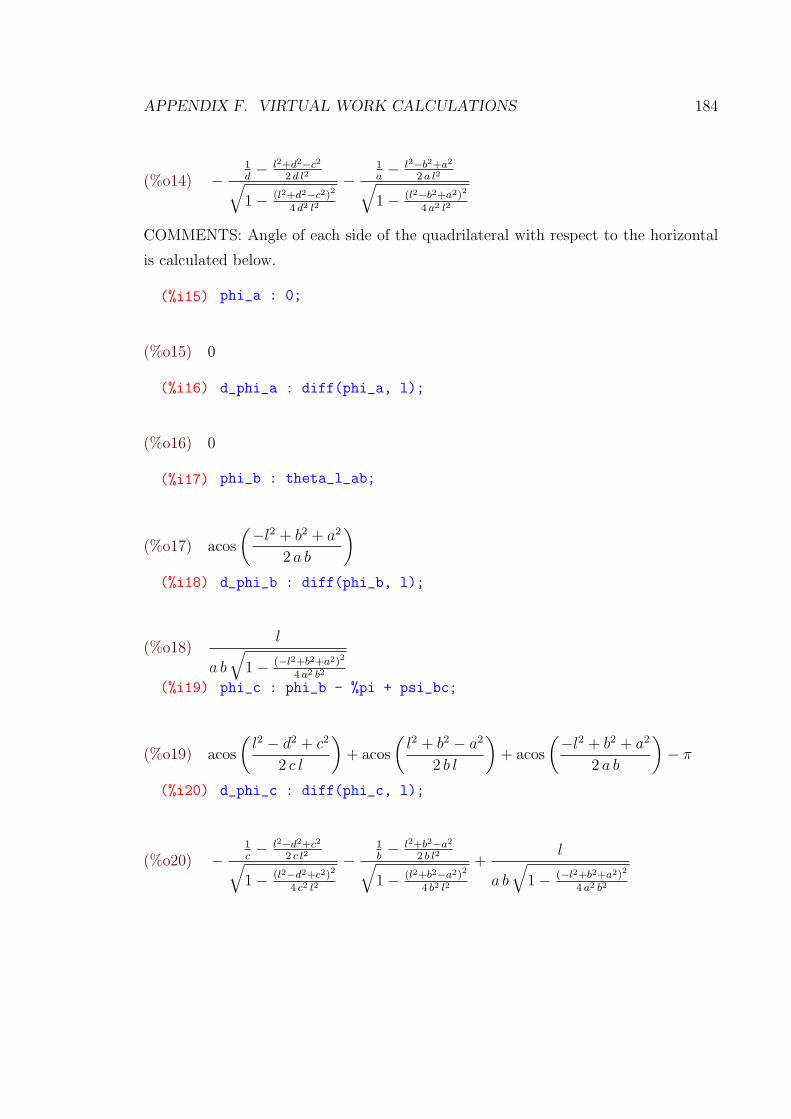
APPENDIX F. VIRTUAL WORK CALCULATIONS 184
(%o14) −1d− l2+d2−c2
2 d l2√
1− (l2+d2−c2)2
4 d2 l2
−1a− l2−b2+a2
2 a l2√
1− (l2−b2+a2)2
4 a2 l2
COMMENTS: Angle of each side of the quadrilateral with respect to the horizontal
is calculated below.
(%i15) phi_a : 0;
(%o15) 0
(%i16) d_phi_a : diff(phi_a, l);
(%o16) 0
(%i17) phi_b : theta_l_ab;
(%o17) acos
(−l2 + b2 + a2
2 a b
)
(%i18) d_phi_b : diff(phi_b, l);
(%o18)l
a b
√
1− (−l2+b2+a2)2
4 a2 b2
(%i19) phi_c : phi_b - %pi + psi_bc;
(%o19) acos
(l2 − d2 + c2
2 c l
)
+ acos
(l2 + b2 − a2
2 b l
)
+ acos
(−l2 + b2 + a2
2 a b
)
− π
(%i20) d_phi_c : diff(phi_c, l);
(%o20) −1c− l2−d2+c2
2 c l2√
1− (l2−d2+c2)2
4 c2 l2
−1b− l2+b2−a2
2 b l2√
1− (l2+b2−a2)2
4 b2 l2
+l
a b
√
1− (−l2+b2+a2)2
4 a2 b2

APPENDIX F. VIRTUAL WORK CALCULATIONS 185
(%i21) phi_d : %pi - psi_da;
(%o21) − acos
(l2 + d2 − c2
2 d l
)
− acos
(l2 − b2 + a2
2 a l
)
+ π
(%i22) d_phi_d : diff(phi_d, l);
(%o22)1d− l2+d2−c2
2 d l2√
1− (l2+d2−c2)2
4 d2 l2
+1a− l2−b2+a2
2 a l2√
1− (l2−b2+a2)2
4 a2 l2
COMMENTS: Numerical values for the sides of the quadrilateral.
(%i23) subss(x):= [a=150/1000, b=100/1000,
c=130/1000, d = 120/1000, l=x];
(%o23) subss (x) := [a =150
1000, b =
100
1000, c =
130
1000, d =
120
1000, l = x]
COMMENTS: The value of l corresponding to the reference configuration, i.e., the
undeformed configuration of the flexure-based four-bar mechanism.
(%i24) l_0 : 140/1000;
(%o24)7
50

APPENDIX F. VIRTUAL WORK CALCULATIONS 186
F.1 Calculation of stiffness in case 3a based on case
2a
F.1.1 Obtaining Fx vs. ux in case 2a using virtual work bal-
ance
COMMENTS: Details of the flexure and calculation of torsional spring constant of
the small-length flexure model.
(%i25) E : 205e9;
(%o25) 2.05 1011
(%i26) flex_width : 500e-6;
(%o26) 5.0000000000000001 10−4
(%i27) flex_thick : 4e-2;
(%o27) 0.04
(%i28) flex_length : 1/100;
(%o28)1
100
(%i29) area_I : 1/12*flex_thick* (flex_width)^3;
(%o29) 4.1666666666666664 10−13
(%i30) kt : E*area_I/flex_length;
(%o30) 8.541666666666666
APPENDIX F. VIRTUAL WORK CALCULATIONS 187
(%i31) subst(subss(l), psi_ab);
(%o31) acos
(
100(
13400
− l2)
3
)
COMMENTS: Virtual work of the torsional springs.
(%i32) virt_wrk_tor_springs :
subst( subss(l),
-1*(
(psi_ab - subst([l=l_0], psi_ab))*d_psi_ab +
(psi_bc - subst([l=l_0], psi_bc))*d_psi_bc +
(psi_cd - subst([l=l_0], psi_cd))*d_psi_cd +
(psi_da - subst([l=l_0], psi_da))*d_psi_da
)
)$
COMMENTS: Rotation matrix.
(%i33) R_mat(theta) := matrix(
[cos(theta),-sin(theta)],
[sin(theta),cos(theta)]
);
(%o33) R mat (θ) :=
(
cos (θ) −sin (θ)
sin (θ) cos (θ)
)
APPENDIX F. VIRTUAL WORK CALCULATIONS 188
(%i34) float(
subst( subss(l_0),
matrix([a], [0]) + R_mat( phi_d). matrix( [d], [0]) +
matrix([0], [-0*flex_length/2])
)
);
(%o34)
(
0.16993795176965
0.11833206699467
)
COMMENTS: Local coordinate of point P on the frame attached to the link associ-
ated with side d.
(%i35) ref_coor_d : float(
subst( subss(l_0),
invert(R_mat( phi_d)).
( R_mat( phi_d). matrix( [d], [0]) + matrix([0], [-flex_length/2]) )
)
);
(%o35)
(
0.11506949720856
−8.3074799040210381 10−4
)
COMMENTS: ux as a function of l
(%i36) ref_displ : matrix([1], [0]) .
( subst( subss(l), R_mat(phi_d).ref_coor_d) -
subst( subss(l_0), R_mat(phi_d).ref_coor_d) )$
COMMENTS: The range of parameter l, on which we focus our interest.

APPENDIX F. VIRTUAL WORK CALCULATIONS 189
(%i37) l_min:94/1000; l_max:170/1000;
(%o37)47
500
(%o38)17
100
(%i39) l_range : [l,l_min,l_max] ;
(%o39) [l,47
500,17
100]
(%i40) plot2d([ref_displ], l_range,
[xlabel, "l (m)"], [ylabel, "u_x (m)"],
[gnuplot_term,ps],[gnuplot_out_file,"./for_thesis_img/ref_displ.eps"])$
-0.03
-0.02
-0.01
0
0.01
0.02
0.03
0.1 0.11 0.12 0.13 0.14 0.15 0.16 0.17
u x (
m)
l (m)
COMMENTS: Virtual work contribution of the horizontal force Fx at point P .

APPENDIX F. VIRTUAL WORK CALCULATIONS 190
(%i41) virt_wrk_ref_force : matrix([1], [0]) .
subst( subss(l) , diff( R_mat(phi_d).ref_coor_d, l) )$
COMMENTS: Explicit expression for Fx in case 2a.
(%i42) f_2a_func_l : kt*virt_wrk_tor_springs/-virt_wrk_ref_force$
(%i43) plot2d([parametric,ref_displ, f_2a_func_l, l_range],
[xlabel, "u_x (m)"], [ylabel, "F_x in case 2a (N)"],
[gnuplot_term,ps],[gnuplot_out_file,"./for_thesis_img/f_2a.eps"] )$
-200
-100
0
100
200
300
400
500
-0.03 -0.02 -0.01 0 0.01 0.02 0.03
Fx
in c
ase
2a (
N)
ux (m)
COMMENTS: Slope of Fx vs. ux at l = l0 in case 2a.
(%i44) f_2a_derivative_l_0 :
float( subst( subss(l_0), diff(f_2a_func_l, l)/diff(ref_displ,l) ) );
(%o44) 5140.246811088702

APPENDIX F. VIRTUAL WORK CALCULATIONS 191
F.1.2 Obtaining Fx vs. ux in case 3a using virtual work bal-
ance
COMMENTS: Coordinates of anchor points, spring displacement, spring force, and
virtual work contribution of spring K21.
(%i45) spring_c_1_glb_anch : matrix( [-0.05], [0.06]);
(%o45)
(
−0.05
0.06
)
(%i46) spring_c_1_local : subst( subss(l_0), matrix( [c/10], [-c/3]) );
(%o46)
(13
1000
− 13300
)
(%i47) spring_c_1_displ : subst( subss(l),
R_mat(phi_b). matrix([b],[0]) + R_mat(phi_c).spring_c_1_local
)$
(%i48) spring_c_1_force :
-spring_c_1_k*(spring_c_1_displ - spring_c_1_glb_anch)$
(%i49) spring_c_1_virt_wrk :
( spring_c_1_force.diff(spring_c_1_displ, l) )$
COMMENTS: Coordinates of anchor points, spring displacement, spring force, and
virtual work contribution of spring K11.
(%i50) spring_b_1_glb_anch : matrix( [0.25], [-0.05] );

APPENDIX F. VIRTUAL WORK CALCULATIONS 192
(%o50)
(
0.25
−0.05
)
(%i51) spring_b_1_local : matrix( [80e-3], [ 0] );
(%o51)
(
0.08
0
)
(%i52) spring_b_1_displ :
subst( subss(l), R_mat(phi_b). spring_b_1_local );
(%o52)
2.666666666666667(
13400
− l2)
0.08
√
1−10000 ( 13
400−l2)
2
9
(%i53) spring_b_1_force :
-spring_b_1_k*(spring_b_1_displ - spring_b_1_glb_anch);
(%o53)
−(2.666666666666667
(13400
− l2)− 0.25
)spring b 1 k
−
(
0.08
√
1−10000 ( 13
400−l2)
2
9+ 0.05
)
spring b 1 k
(%i54) spring_b_1_virt_wrk : spring_b_1_force . diff(spring_b_1_displ, l)$
COMMENTS: By virtual work balance, Fx in case 3a is explicitly written as below.
Note that it is a function of l with spring constants of K11 (spring b 1 k) and K2
1
(spring c 1 k) being unknowns.
(%i55) f_3a_func_l_unit_k :
(spring_c_1_virt_wrk + spring_b_1_virt_wrk )/-virt_wrk_ref_force$
COMMENTS: Fx and slope of Fx vs. ux at l = l0.

APPENDIX F. VIRTUAL WORK CALCULATIONS 193
(%i56) f_3a_func_l_unit_k_origin :
expand( float( subst( subss(l_0), f_3a_func_l_unit_k) ) );
(%o56) 0.14647046533381 spring c 1 k − 0.2461002568181 spring b 1 k
(%i57) f_3a_func_l_unit_k_derivative :
expand( float(
subst(subss(l_0),
diff( f_3a_func_l_unit_k, l) / diff(ref_displ ,l ) )
) );
(%o57) 2.58328234272209 spring c 1 k − 1.37850044099567 spring b 1 k
COMMENTS: Equating Fx and slope of Fx vs. ux at l = l0 between case 2a and case
3a, the stiffness of springs K21 (spring c 1 k) and K1
1 (spring b 1 k) are solved below.
(%i58) spring_cnst_sub: float(
solve(
[f_3a_func_l_unit_k_origin=0,
f_3a_func_l_unit_k_derivative=f_2a_derivative_l_0 ],
[spring_c_1_k, spring_b_1_k])
);
rat : replaced−0.2461002568181by−1625/6603 = −0.2461002574587rat : replaced0.14647046533381
0.14647046501885rat : replaced−5140.2468110887by−395799/77 = −5140.24675324675rat :
replaced−1.37850044099567by−1526/1107 = −1.37850045167118rat : replaced2.58328234272209
2.583282302510717
(%o58) [[spring c 1 k = 2915.879749896249, spring b 1 k = 1735.432003674265]]

APPENDIX F. VIRTUAL WORK CALCULATIONS 194
(%i59) plot2d([[parametric,ref_displ, f_2a_func_l, l_range] ,
[ parametric,
ref_displ,
subst(spring_cnst_sub , f_3a_func_l_unit_k) ,
l_range]
],
[xlabel, "u_x (m)"], [ylabel, "F_x (N)"],
[legend, "case 2a", "case 3a"],
[gnuplot_term,ps],
[gnuplot_out_file,"./for_thesis_img/f_2a_f_3a.eps"] );
(%o59)
-200
-100
0
100
200
300
400
500
-0.03 -0.02 -0.01 0 0.01 0.02 0.03
Fx
(N
)
ux (m)
case 2acase 3a

APPENDIX F. VIRTUAL WORK CALCULATIONS 195
F.2 Verification of static balance in case 3b through
virtual work balance
(%i60) spring_c_2_glb_anch : spring_c_1_glb_anch;
(%o60)
(
−0.05
0.06
)
(%i61) spring_c_2_local : -spring_c_1_local$
(%i62) spring_c_2_displ : subst( subss(l),
R_mat(phi_b). matrix([b],[0]) + R_mat(phi_c).spring_c_2_local
)$
(%i63) float( subst( subss(l_0), spring_c_2_displ ) );
(%o63)
(
0.020956478739549
0.12979062150905
)
(%i64) spring_c_2_force :
-spring_c_2_k*(spring_c_2_displ - spring_c_2_glb_anch)$
(%i65) spring_c_2_virt_wrk :
( spring_c_2_force.diff(spring_c_2_displ, l) )$
(%i66) spring_b_2_glb_anch :
matrix( [-0.00916760640646499], [ -0.04633295743741400] );
(%o66)
(
−0.009167606406465
−0.046332957437414
)
APPENDIX F. VIRTUAL WORK CALCULATIONS 196
(%i67) spring_b_2_local : matrix( [80e-3], [ 0] );
(%o67)
(
0.08
0
)
(%i68) spring_b_2_displ :
subst( subss(l), R_mat(phi_b). spring_b_2_local )$
(%i69) float( subst( subss(l_0), spring_b_2_displ ) );
(%o69)
(
0.0344
0.072226310995371
)
(%i70) spring_b_2_force :
-spring_b_2_k*(spring_b_2_displ - spring_b_2_glb_anch)$
(%i71) spring_b_2_virt_wrk :
spring_b_2_force . diff(spring_b_2_displ, l);
(%o71) 5.333333333333333 l
(
2.666666666666667
(13
400− l2
)
+ 0.009167606406465
)
spring b
177.7777777777778 l(
13400
− l2)
(
0.08
√
1−10000 ( 13
400−l2)
2
9+ 0.046332957437414
)
spring b 2 k
√
1−10000 ( 13
400−l2)
2
9
(%i72) bal_sprng_cnst :
[spring_c_2_k= 2915.87974989625, spring_b_2_k= 7567.19150346676 ];
(%o72) [spring c 2 k = 2915.87974989625, spring b 2 k = 7567.19150346676]

APPENDIX F. VIRTUAL WORK CALCULATIONS 197
(%i73) f_bal_func_l_unit_k :
(spring_c_2_virt_wrk + spring_b_2_virt_wrk )/-virt_wrk_ref_force$
(%i74) plot2d([[parametric,ref_displ,
( subst(spring_cnst_sub , f_3a_func_l_unit_k)
+ subst( bal_sprng_cnst, f_bal_func_l_unit_k) ) ,
l_range] ,
[ parametric,
ref_displ,
subst(spring_cnst_sub , f_3a_func_l_unit_k) ,
l_range],
[ parametric,
ref_displ,
subst( bal_sprng_cnst, f_bal_func_l_unit_k) ,
l_range]
],
[xlabel, "u_x (m)"], [ylabel, "F_x (N)"],
[legend, "case 3b", "case 3a", "balancing springs"],
[gnuplot_term,ps],
[gnuplot_out_file,"./for_thesis_img/f_2a_f_3a_balnce_contri.eps"]
);
(%o74)
COMMENTS: The following plot shows that virtual work contribution of original
springs and balancing springs in case 3b is zero over the range of l that is plotted.
This signify that static balance has indeed been attained.
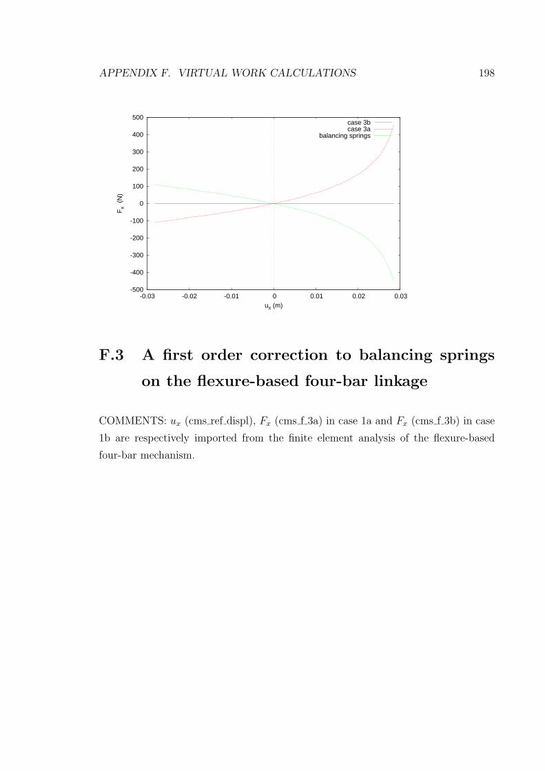
APPENDIX F. VIRTUAL WORK CALCULATIONS 198
-500
-400
-300
-200
-100
0
100
200
300
400
500
-0.03 -0.02 -0.01 0 0.01 0.02 0.03
Fx
(N
)
ux (m)
case 3bcase 3a
balancing springs
F.3 A first order correction to balancing springs
on the flexure-based four-bar linkage
COMMENTS: ux (cms ref displ), Fx (cms f 3a) in case 1a and Fx (cms f 3b) in case
1b are respectively imported from the finite element analysis of the flexure-based
four-bar mechanism.

APPENDIX F. VIRTUAL WORK CALCULATIONS 199
(%i75) cms_ref_displ : [
-0.025 ,
-0.022619047619047622 ,
-0.02023809523809524 ,
-0.017857142857142856 ,
-0.015476190476190477 ,
-0.013095238095238096 ,
-0.010714285714285714 ,
-0.008333333333333331 ,
-0.005952380952380952 ,
-0.0035714285714285726,
-0.0011904761904761897,
0.0011904761904761932 ,
0.0035714285714285726 ,
0.005952380952380952 ,
0.008333333333333338 ,
0.010714285714285718 ,
0.013095238095238097 ,
0.015476190476190477 ,
0.017857142857142856 ,
0.020238095238095243 ,
0.022619047619047622 ,
0.025 ]$

APPENDIX F. VIRTUAL WORK CALCULATIONS 200
(%i76) cms_f_3a : [ -104.34594127214568 ,
-95.50949264952318 ,
-86.56303274592234 ,
-77.47330027942202 ,
-68.20345749702217 ,
-58.712126896397784 ,
-48.952203085118825 ,
-38.86932451582366 ,
-28.399875264975144 ,
-17.46832758018575 ,
-5.983643468057328 ,
6.165693524475422 ,
19.118685721280066 ,
33.05194222684286 ,
48.19469250388112 ,
64.8517456852825 ,
83.4398521812106 ,
104.54768638980624 ,
129.03965467289203 ,
158.24607605283924 ,
194.33613042898966 ,
241.11064684981028 ]$
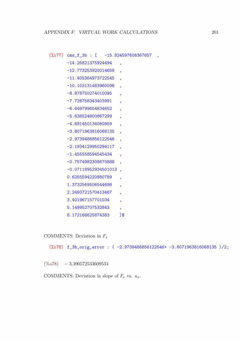
APPENDIX F. VIRTUAL WORK CALCULATIONS 201
(%i77) cms_f_3b : [ -15.824597608367657 ,
-14.25821375924494 ,
-12.773253920014659 ,
-11.405364973722545 ,
-10.103131463960098 ,
-8.878750274010095 ,
-7.728758343403991 ,
-6.649799654834652 ,
-5.638524800867299 ,
-4.691450134080959 ,
-3.8071963816068135 ,
-2.9739486856122546 ,
-2.1934129950294117 ,
-1.455558594545434 ,
-0.7574982308670888 ,
-0.07118952934501013 ,
0.6255594220880789 ,
1.3732569506544698 ,
2.2493721570413467 ,
3.401967157701034 ,
5.149952707532843 ,
8.172168625874383 ]$
COMMENTS: Deviation in Fx
(%i78) f_3b_orig_error : ( -2.9739486856122546+ -3.8071963816068135 )/2;
(%o78) − 3.390572533609534
COMMENTS: Deviation in slope of Fx vs. ux.

APPENDIX F. VIRTUAL WORK CALCULATIONS 202
(%i79) f_3b_slope_error :
( -2.9739486856122546- -3.8071963816068135 )/
( 0.0011904761904761932 - -0.0011904761904761932);
(%o79) 349.964032317714
COMMENTS: Two linear equations defining the first order correction on k22 (spring c 2 k)
and k12 (spring b 2 k).
(%i80) correc_eq_1 :float( expand(
subst( subss(l_0), f_bal_func_l_unit_k)
) ) =
-f_3b_orig_error;
(%o80) 0.030088976858302 spring c 2 k−0.011594240624521 spring b 2 k = 3.390572533609534
(%i81) correc_eq_2 : float( expand(
subst( subss(l_0),
diff(f_bal_func_l_unit_k,l)/ diff(ref_displ ,l ) )
) )
=-f_3b_slope_error;
(%o81) −0.028273987618258 spring c 2 k−0.66838579798129 spring b 2 k = −349.964032317714
COMMENTS: The two equations are solved for the correction in stiffness of the
balancing springs.
(%i82) float( solve(
[correc_eq_1, correc_eq_2],
[spring_c_2_k, spring_b_2_k]) );
rat : replaced−3.39057253360953by−79770/23527 = −3.3905725336847rat : replaced−

APPENDIX F. VIRTUAL WORK CALCULATIONS 203
0.01159424062452by−889/76676 = −0.01159424070113rat : replaced0.030088976858302by443/14723
0.030088976431434rat : replaced349.964032317714by48645/139 = 349.9640287769784rat :
replaced − 0.6683857979813by − 9979/14930 = −0.6683858004019rat : replaced −
0.02827398761826by − 1415/50046 = −0.0282739879311
(%o82) [[spring c 2 k = 309.3997276682762, spring b 2 k = 510.5076505303351]]
COMMENTS: Finite element analysis data of Fx after the correction.
(%i83) cms_3b_post_correc : [
-6.909034235038472 ,
-5.83429860238359 ,
-4.874566950191206 ,
-4.01833402821449 ,
-3.264279702980125 ,
-2.6117285115315623 ,
-2.0606882689860524 ,
-1.6119039235596984 ,
-1.2669288585698968 ,
-1.0282162854171706 ,
-0.9025937472472608 ,
-0.888930983768344 ,
-0.9902145311237647 ,
-1.2313346408838126 ,
-1.6044520551744579 ,
-2.1266404020078657 ,
-2.81101615779267 ,
-3.671581877007283 ,
-4.719935737519259 ,
-5.954192496041346 ,
-7.317875319092065 ,
-8.74382642287233 ]$

APPENDIX F. VIRTUAL WORK CALCULATIONS 204
(%i84) plot2d([[parametric,ref_displ, f_2a_func_l, l_range] ,
[ parametric,
ref_displ,
subst(spring_cnst_sub , f_3a_func_l_unit_k) ,
l_range],
[ parametric,
ref_displ,
f_2a_func_l+subst( bal_sprng_cnst, f_bal_func_l_unit_k) ,
l_range] ,
[ parametric,
ref_displ,
subst(spring_cnst_sub , f_3a_func_l_unit_k) +
subst( bal_sprng_cnst, f_bal_func_l_unit_k) ,
l_range],
[discrete, cms_ref_displ, cms_f_3a],
[discrete, cms_ref_displ, cms_f_3b],
[discrete, cms_ref_displ,cms_3b_post_correc ]],
[legend, "f2a", "f3a", "f2b", "f3b", "f1a", "f1b", "f1c" ],
[xlabel, "generalized displacement [m]"],
[ylabel, "generalized force [N]"],
[gnuplot_term,ps],[gnuplot_out_file,"case_plots.eps"]);
(%o84)
(%i85) load(draw)$
(%i86) case_1a : points(cms_ref_displ, cms_f_3a)$
(%i87) case_1b : points(cms_ref_displ, cms_f_3b)$

APPENDIX F. VIRTUAL WORK CALCULATIONS 205
(%i88) case_1c : points( cms_ref_displ,cms_3b_post_correc)$
(%i89) case_2a : parametric(ref_displ,
f_2a_func_l, l, l_min, l_max)$
(%i90) case_2b : parametric(ref_displ,
f_2a_func_l+
subst( bal_sprng_cnst, f_bal_func_l_unit_k),
l, l_min, l_max)$
(%i91) case_3a : parametric(ref_displ,
subst(spring_cnst_sub , f_3a_func_l_unit_k) ,
l, l_min, l_max)$
(%i92) case_3b : parametric( ref_displ,
subst(spring_cnst_sub , f_3a_func_l_unit_k) +
subst( bal_sprng_cnst, f_bal_func_l_unit_k) ,
l, l_min, l_max)$
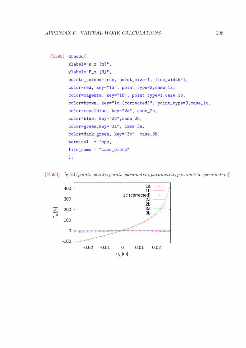
APPENDIX F. VIRTUAL WORK CALCULATIONS 206
(%i93) draw2d(
xlabel="u_x [m]",
ylabel="F_x [N]",
points_joined=true, point_size=1, line_width=1,
color=red, key="1a", point_type=2,case_1a,
color=magenta, key="1b", point_type=1,case_1b,
color=brown, key="1c (corrected)", point_type=3,case_1c,
color=royalblue, key="2a", case_2a,
color=blue, key="2b",case_2b,
color=green,key="3a", case_3a,
color=dark-green, key="3b", case_3b,
terminal = ’eps,
file_name = "case_plots"
);
(%o93) [gr2d (points, points, points, parametric, parametric, parametric, parametric)]
-100
0
100
200
300
400
-0.02 -0.01 0 0.01 0.02
Fx
[N]
ux [m]
1a1b
1c (corrected)2a2b3a3b

Appendix G
Static balancing of compliant
mechanisms using rigid-body
linkages and springs
Figure (G.1) shows a compliant gripper that is statically balanced with a small 2R
linkage loaded by a zero-free-length spring. The zero-free-length spring is realized by
a pulley-string arrangement.
In order to understand the principle behind the static balance in figure (G.1), con-
sider figures (G.2) and (G.3). Figure (G.2a) shows a statically balanced parallelogram
(for details see figure (2.6)). The spring between between B and D in figure (G.2a) is
relocated to be between E and A, as shown in figure (G.2b), where−−→BC =
−−→EB. From
geometry, it follows that this relocation does not change the length of the spring and
hence does not change the potential energy. Therefore the linkage of figure (G.2b) is
also statically balanced.
Figure (G.3) shows a compliant gripper, which is actuated by pulling down the
actuator rod shown in the figure. The actuator rod is guided to maintain symmetric
actuation. Because of the guide and the inherent elasticity of the compliant mecha-
nism, the actuator rod behaves as a one-dimensional spring. We found that for the
range of operation of the compliant mechanism, the force-displacement relation is
linear for practical purposes.
207

APPENDIX G. ANOTHER COMPLIANT MECHANISM BALANCING 208
Figure G.1: A compliant gripper compensated by a small spring loaded 2R linkage.(Basement board dimension: 2.5 feet × 2.5 feet)

APPENDIX G. ANOTHER COMPLIANT MECHANISM BALANCING 209
l
k
l
l
k
k
(a)
(b)
kA
B
C
D
A
B
C
E
Figure G.2: A statically balanced parallelogram and its modification

APPENDIX G. ANOTHER COMPLIANT MECHANISM BALANCING 210
Figure G.3: A compliant gripper

APPENDIX G. ANOTHER COMPLIANT MECHANISM BALANCING 211
If we replace the spring between A and E, in figure (G.2b) by the actuator rod
with the stiffness of the spring between C and A matching that of the actuator rod,
we get the setup shown in figure (G.1). Since the linkage in figure (G.2b) is statically
balanced, the setup in figure (G.1) is also statically balanced. We had demonstrated
this set up in a few places and people invariably felt the difference between the
actuation effort before and after balancing to be dramatic.

Appendix H
Impossibility of statically balancing
a tree-structured gravity-loaded
rigid-body linkage by adding
springs only between successive
links
In the static balancing method of Chapter 5, the balancing springs were always at-
tached from the root to different parts of the linkage. In the case of gravity-loaded
linkages, the root is the ground. A question may arise about the possibility of stat-
ically balancing gravity-loaded tree-structured linkages without using auxiliary links
with springs added only between successive links of the tree-structure. In this ap-
pendix, we show that such a thing is not possible.
Let i be a terminal body of a tree-structured linkage, as shown in figure H.1.
Let p[i] be the center of gravity in the local coordinate frame and f [i] be the net
gravitational force. Then, the potential energy due to the gravity load takes the
form:
PEgravityi = −f [i]TR(θ[i])p[i] − f [i]Tr[i] (H.1)
212

APPENDIX H. SPRINGS BETWEEN SUCCESSIVE LINKS 213
0
i
j
x
y
θ[i]
x[i]
y[i]
r[i]
x
p[i]
f [i]
Figure H.1: A tree-structured linkage under gravity load
The terms dependent on θ[i] in equation H.1 are sinusoidal since f [i] and p[i] are
constants. Hence, equation (H.1) may be rewritten as:
PEgravityi = a cos(θ[i] + α
)− f [i]Tr[i] (H.2)
where a, α and f [i] are constants.
Suppose that static balance is achieved by adding balancing springs, of some type,
attached only between successive links. Two links are successive if they are connected
by a joint. Then, the net potential energy of the springs connected between body i
and its parent j depends on the relative angle between the two, i.e.,
PEspringij = Ψ(θ[i] − θ[j]
)(H.3)
Apart from θ[i], let all the configuration parameters of the linkage be fixed at some
value. In particular, let r[i] be r1 and θ[j] be γ1. Here, we assume that body j is
not the root. It means that the tree topology of linkage should have more than one
generation. Then, for the entire linkage, the only varying potential energy components

APPENDIX H. SPRINGS BETWEEN SUCCESSIVE LINKS 214
are:
a cos(θ[i] + α
)and Ψ
(θ[i] − γ1
)
These components should sum up to a constant since a linkage that is statically bal-
anced continues to be statically balanced even when any of the configuration variables
are fixed or constrained in any manner. Hence, we have have
a cos(θ[i] + α
)+Ψ
(θ[i] − γ1
)= C1 (H.4)
which may be further rewritten as
Ψ(θ[i] − γ1
)= −a cos
(θ[i] + α
)+ C1 (H.5)
Similarly, it is possible to fix the configuration variables, apart from θ[i] at some
different values. In particular, let θ[j] be fixed at γ2 with γ1 6= γ2. In this situation
also, similar to equation (H.5), we can write
Ψ(θ[i] − γ2
)= −a cos
(θ[i] + α
)+ C2 (H.6)
Further, equation (H.5) is true for any θ[i]. In particular, it is true for(θ[i] − (γ2 − γ1)
)
as well. Hence, equation (H.5), may be written as
Ψ(θ[i] − (γ2 − γ1)− γ1
)= Ψ
(θ[i] − γ2
)= −a cos
(θ[i] − (γ2 − γ1) + α
)+ C1 (H.7)
From equations (H.6) and (H.7), we have
a cos(θ[i] + α
)= a cos
(θ[i] + α− (γ2 − γ1)
)+ C2 − C1 (H.8)
What the above equation says is that when there is any non-zero phase shift in the
sinusoidal function, the function changes only by a constant. This is clearly a con-
tradiction. Hence, the statement that static balance is achieved by adding balancing
springs, of some type, connected only between successive links is false. In other
words, it is impossible to statically balance a gravity loaded tree-structured (having

APPENDIX H. SPRINGS BETWEEN SUCCESSIVE LINKS 215
more than one generation) linkage by adding springs, of whatever type, between only
successive links.
Bibliography
[1] J. L. Herder, “Design of spring force compensation systems,” Mechanisms and
Machine Theory, vol. 33, no. 1, pp. 151–161, 1998.
[2] M. French and M. Widden, “The spring-and-lever balancing mechanism, george
carwardine and the anglepoise lamp,” Proceedings of the Institution of Mechan-
ical Engineers, Part C: Journal of Mechanical Engineering Science, vol. 214,
no. 3, pp. 501–508, 2000.
[3] L. J. B. LaCoste Jr., “A new type long period vertical seismograph,” Journal of
Applied Physics, vol. 5, no. 7, pp. 178–180, 1934.
[4] J. L. Herder, Energy-free Systems: Theory, conception and design of statically
balanced spring mechanisms. PhD dissertation, Delft University of Technology,
2001. ISBN 90-370-0192-0.
[5] D. A. Streit and B. J. Gilmore, “Perfect spring equilibrators for rotatable bod-
ies,” ASME Journal of Mechanisms, Transmissions, and Automation in Design,
vol. 111, pp. 451–458, December 1989.
[6] L. L. Howell and A. Midha, “Parametric deflection approximations for end-
loaded, large-deflection beams in compliant mechanisms,” ASME Journal of Me-
chanical Design, vol. 117, pp. 156–165, March 1995.
[7] L. L. Howell and A. Midha, “A method for the design of compliant mechanisms
with small-length flexural pivots,” Journal of Mechanical Design, vol. 116, no. 1,
pp. 280–290, 1994.
216

BIBLIOGRAPHY 217
[8] S. R. Deepak and G. Ananthasuresh, “Static balancing of a four-bar linkage and
its cognates,” Mechanism and Machine Theory, vol. 48, no. 0, pp. 62 – 80, 2012.
[9] H. de Visser and J. L. Herder, “Force-directed design of a voluntary closing
hand prosthesis,” Journal of Rehabilitation Research and Development, vol. 37,
pp. 261–271, May/June 2000.
[10] K. H. Hunt, Kinematic geometry of mechanisms. Oxford University Press, Ox-
ford, 1978.
[11] S. Stein, Archimedes: what did he do besides cry eureka? Mathematical Associ-
ation of America, 1999.
[12] “Balanced-arm lamp,” December 2011. Wikipedia, the free encyclopedia.
[13] J. Wang and C. M. Gosselin, “Static balancing of spatial three-degree-of-freedom
parallel mechanisms,” Mechanism and Machine Theory, vol. 34, no. 3, pp. 437 –
452, 1999.
[14] G. Carwardine, “Improvements in elastic force mechanisms,” 1932. UK Patent
379 680.
[15] G. Carwardine, “Improvements in elastic equipoising mechanisms,” 1934. UK
Patent 404 615.
[16] G. Carwardine, “Improvements in equipoising mechanism,” 1935. UK Patent
433 617.
[17] G. Carwardine, “Equipoising mechanism,” Aug. 17 1937. US Patent 2,090,439.
[18] G. Carwardine, “Equipoising mechanism,” Apr. 6 1937. US Patent 2,076,446.
[19] R. M. Nathan, “A constant force generation mechanism,” ASME Journal of
Mechanisms, Transmissions, and Automation in Design, vol. 107, pp. 508–512,
December 1985.
BIBLIOGRAPHY 218
[20] P. Pracht, P. Minotti, and M. Dahan, “Synthesis and balancing of cam-odulated
linkages.,” in American Society of Mechanical Engineers, Design Engineering
Division (Publication) DE, vol. 10-2, pp. 221–226, 1987.
[21] E. Shin and D. A. Streit, “Spring equilibrator theory for static balancing of
planar pantograph linkages,” Mechanism and Machine Theory, vol. 26, no. 7,
pp. 645 – 657, 1991.
[22] T. Wongratanaphisan and M. Cole, “Analysis of a gravity compensated four-bar
linkage mechanism with linear spring suspension,” Journal of Mechanical Design,
vol. 130, p. 011006, 2008.
[23] D. A. Streit and E. Shin, “Equilibrators for planar linkages,” ASME Journal of
Mechanical Design, vol. 115, pp. 604–611, September 1993.
[24] G. Walsh, D. Streit, and B. Gilmore, “Spatial spring equilibrator theory,” Mech-
anism and Machine Theory, vol. 26, no. 2, pp. 155 – 170, 1991.
[25] D. A. Streit, H. Chung, and B. J. Gilmore, “Perfect equilibrators for rigid body
spatial rotations about a hooke’s joint,” Journal of Mechanical Design, vol. 113,
no. 4, pp. 500–507, 1991.
[26] T. Wongratanaphisan and M. Chew, “Gravity compensation of spatial two-dof
serial manipulators,” Journal of Robotic Systems, vol. 19, no. 7, pp. 329–347,
2002.
[27] S. K. Agrawal and A. Fattah, “Gravity-balancing of spatial robotic manipula-
tors,” Mechanism and Machine Theory, vol. 39, no. 12, pp. 1331 – 1344, 2004.
[28] T. Rahman, R. Ramanathan, R. Seliktar, andW. Harwin, “A simple technique to
passively gravity-balance articulated mechanisms,” Transactions-American So-
ciety Of Mechanical Engineers Journal Of Mechanical Design, vol. 117, pp. 655–
657, 1995.
BIBLIOGRAPHY 219
[29] P.-Y. Lin, W.-B. Shieh, and D.-Z. Chen, “Design of a gravity-balanced general
spatial serial-type manipulator,” Journal of Mechanisms and Robotics, vol. 2,
no. 3, p. 031003, 2010.
[30] J. Wang and C. M. Gosselin, “Static balancing of spatial four-degree-of-freedom
parallel mechanisms,” Mechanism and Machine Theory, vol. 35, no. 4, pp. 563 –
592, 2000.
[31] T. Laliberte, C. M. Gosselin, and M. Jean, “Static balancing of 3-dof planar par-
allel mechanisms,” IEEE/ASME Transactions On Mechatronics, vol. 4, pp. 363–
377, 1999.
[32] C. M. Gosselin and J. Wang, “Static balancing of spatial six-degree-of-freedom
parallel mechanisms with revolute actuators,” Journal of Robotic Systems,
vol. 17, no. 3, pp. 159–170, 2000.
[33] I. Ebert-Uphoff, C. M. Gosselin, and T. Laliberte, “Static balancing of spa-
tial parallel platform mechanisms—revisited,” Journal of Mechanical Design,
vol. 122, no. 1, pp. 43–51, 2000.
[34] C. Gosselin, “Static balancing of spherical 3-dof parallel mechanisms and manip-
ulators,” The International Journal of Robotics Research, vol. 18, no. 8, pp. 819–
829, 1999.
[35] A. Russo, R. Sinatra, and F. Xi, “Static balancing of parallel robots,” Mechanism
and Machine Theory, vol. 40, no. 2, pp. 191–202, 2005.
[36] C. Gosselin and J. Wang, “On the design of gravity-compensated six-degree-of-
freedom parallel mechanisms,” in Robotics and Automation, 1998. Proceedings.
1998 IEEE International Conference on, vol. 3, pp. 2287–2294, IEEE, 1998.
[37] I. Ebert-Uphoff and K. Johnson, “Practical considerations for the static bal-
ancing of mechanisms of parallel architecture,” Proceedings of the Institution of
Mechanical Engineers, Part K: Journal of Multi-body Dynamics, vol. 216, no. 1,
pp. 73–85, 2002.

BIBLIOGRAPHY 220
[38] M. Jean and C. Gosselin, “Static balancing of planar parallel manipulators,” in
Robotics and Automation, 1996. Proceedings., 1996 IEEE International Confer-
ence on, vol. 4, pp. 3732–3737, IEEE, 1996.
[39] S. Deepak and G. K. Ananthasuresh, “Static balancing of spring-loaded planar
revolute-joint linkages without auxiliary links,” in 14th National Conference on
Machines and Mechanisms, 2009. December 17-18, NIT, Durgapur, India.
[40] P.-Y. Lin, W.-B. Shieh, and D.-Z. Chen, “A stiffness matrix approach for the
design of statically balanced planar articulated manipulators,” Mechanism and
Machine Theory, vol. 45, no. 12, pp. 1877 – 1891, 2010.
[41] W. Shieh and D. Chen, “Design of perfectly statically balanced one-dof pla-
nar linkages with revolute joints only,” Journal of Mechanical Design, vol. 131,
pp. 051004–1, 2009.
[42] S. R. Deepak and G. K. Ananthasuresh, “Perfect static balance of linkages by ad-
dition of springs but not auxiliary bodies,” Journal of Mechanisms and Robotics,
vol. 4, no. 2, p. 021014, 2012.
[43] A. Gopalswamy, P. Gupta, and M. Vidyasagar, “A new parallelogram linkage
configuration for gravity compensation using torsional springs,” in Proceedings
of the 1992 IEEE International Conference on Robotics and Automation, (Nice,
France), May 1992.
[44] A. Agrawal and S. Agrawal, “Design of gravity balancing leg orthosis using non-
zero free length springs,” Mechanism and Machine Theory, vol. 40, pp. 693–709,
2005.
[45] N. Ulrich and V. Kumar, “Passive mechanical gravity compensation for robot
manipulators,” in Proceedings of the 1991 IEEE International Conference on
Robotics and Automation, (Sacramento, California), April 1991.
[46] F. te Riele and J. Herder, “Perfect static balance with normal springs,” in
Proceedings of the ASME Design Engineering Technical Conferences, Pittsburg,
Pennsylvania, pp. 9–12, 2001.

BIBLIOGRAPHY 221
[47] K. Koser, “A cam mechanism for gravity-balancing,” Mechanics Research Com-
munications, vol. 36, no. 4, pp. 523 – 530, 2009.
[48] S. Agrawal and A. Fattah, “Theory and design of an orthotic device for full or
partial gravity-balancing of a human leg during motion,” IEEE Transactions on
Neural Systems and Rehabilitation Engineering, vol. 12, no. 2, pp. 157–165, 2004.
[49] S. Banala, S. Agrawal, A. Fattah, K. Rudolph, and J. Scholz, “A gravity balanc-
ing leg orthosis for robotic rehabilitation,” in Robotics and Automation, 2004.
Proceedings. ICRA’04. 2004 IEEE International Conference on, vol. 3, pp. 2474–
2479, IEEE, 2004.
[50] S. Banala, S. Agrawal, A. Fattah, V. Krishnamoorthy, W. Hsu, J. Scholz, and
K. Rudolph, “Gravity-balancing leg orthosis and its performance evaluation,”
IEEE Transactions on Robotics, vol. 22, no. 6, pp. 1228–1239, 2006.
[51] V. Arakelian and S. Ghazaryan, “Improvement of balancing accuracy of robotic
systems: Application to leg orthosis for rehabilitation devices,” Mechanism and
Machine Theory, vol. 43, no. 5, pp. 565–575, 2008.
[52] A. Agrawal and S. K. Agrawal, “Design of gravity balancing leg orthosis using
non-zero free length springs,” Mechanism and Machine Theory, vol. 40, no. 6,
pp. 693 – 709, 2005.
[53] S. Agrawal, A. Fattah, and S. Banala, “Design and prototype of a gravity-
balanced leg orthosis,” International Journal of Humanfriendly Welfare Robotic
Systems, pp. 13–16, 2003.
[54] A. Fattah and S. Agrawal, “Gravity balancing rehabilitative robot for the human
legs,” in Engineering in Medicine and Biology Society, 2004. IEMBS’04. 26th
Annual International Conference of the IEEE, vol. 1, pp. 2695–2698, IEEE, 2004.
[55] S. Agrawal, S. Banala, A. Fattah, V. Sangwan, V. Krishnamoorthy, J. Scholz,
and H. Wei-Li, “Assessment of motion of a swing leg and gait rehabilitation

BIBLIOGRAPHY 222
with a gravity balancing exoskeleton,” IEEE Transactions on Neural Systems
and Rehabilitation Engineering, vol. 15, no. 3, pp. 410–420, 2007.
[56] S. Agrawal, S. Banala, A. Fattah, J. Scholz, V. Krishnamoorthy, and W. Hsu,
“A gravity balancing passive exoskeleton for the human leg,” in Proceedings of
Robotics: Science and Systems, 2006.
[57] J. Herder, “Development of a statically balanced arm support: Armon,” in
Rehabilitation Robotics, 2005. ICORR 2005. 9th International Conference on,
pp. 281–286, IEEE, 2005.
[58] J. Herder, N. Vrijlandt, T. Antonides, M. Cloosterman, P. Mastenbroek, et al.,
“Principle and design of a mobile arm support for people with muscular weak-
ness,” Journal of rehabilitation research and development, vol. 43, no. 5, p. 591,
2006.
[59] R. Rizk, S. Krut, and E. Dombre, “Design of a 3d gravity balanced orthosis for
upper limb,” in Robotics and Automation, 2008. ICRA 2008. IEEE International
Conference on, pp. 2447–2452, IEEE, 2008.
[60] S. Agrawal and A. Fattah, “Design of an orthotic device for full or partial gravity-
balancing of a human upper arm during motion,” in Intelligent Robots and Sys-
tems, 2003.(IROS 2003). Proceedings. 2003 IEEE/RSJ International Conference
on, vol. 3, pp. 2841–2846, IEEE, 2003.
[61] A. Stienen, E. Hekman, F. Van der Helm, G. Prange, M. Jannink, A. Aalsma,
and H. Van der Kooij, “Freebal: dedicated gravity compensation for the upper
extremities,” in Rehabilitation Robotics, 2007. ICORR 2007. IEEE 10th Inter-
national Conference on, pp. 804–808, IEEE, 2007.
[62] P. Lin, W. Shieh, and D. Chen, “Design of statically balanced planar articulated
manipulators with spring suspension,” IEEE Transactions on Robotics, vol. 28,
no. 1, pp. 12–21, 2012.
BIBLIOGRAPHY 223
[63] P. Lin, W. Shieh, and D. Chen, “A theoretical study of weight-balanced mecha-
nisms for design of spring assistive mobile arm support (mas),” Mechanism and
Machine Theory, vol. 61, pp. 156–167, 2013.
[64] L. L. Howell, Compliant Mechanisms. John Wiley and Sons, Inc., 2001.
[65] G. Radaelli, J. A. Gallego, and J. L. Herder, “An energy approach to static bal-
ancing of systems with torsion stiffness,” Journal of Mechanical Design, vol. 133,
no. 9, p. 091006, 2011.
[66] J. L. Herder and F. P. A. van den Berg, “Statically balanced compliant mecha-
nisms (sbcm’s), an example and prospects,” in Proceedings ASME DETC 26th
Biennial Mechanisms and Robotics Conference, (Baltimore, Maryland), Septem-
ber 2000. Paper number: DETC2000/MECH-14144.
[67] A. Stapel and J. L. Herder, “Feasibility study of a fully compliant statically bal-
anced laparoscopic grasper,” ASME Conference Proceedings, vol. 2004, no. 46954,
pp. 635–643, 2004.
[68] N. Tolou and J. L. Herder, “Concept and modeling of a statically balanced
compliant laparoscopic grasper,” ASME Conference Proceedings, vol. 2009,
no. 49040, pp. 163–170, 2009.
[69] D. J. B. A. de Lange, M. Langelaar, and J. L. Herder, “Design of a statically bal-
anced compliant grasper using topology optimization,” in ASME International
Design Engineering Technical Conferences, (New York), August 2008. Paper
number: DETC2008-49794.
[70] D. J. B. A. De Lange, M. Langelaar, and J. L. Herder, “Towards the design of a
statically balanced compliant laparoscopic grasper using topology optimization,”
in Proceedings of the ASME Design Engineering Technical Conference, vol. 2,
pp. 293–305, 2008.
[71] F. M. Morsch and J. L. Herder, “Design of a generic zero stiffness compliant
joint,” in Proceedings of the ASME Design Engineering Technical Conference,
vol. 2, pp. 427–435, 2010.

BIBLIOGRAPHY 224
[72] K. Hoetmer, G. Woo, C. Kim, and J. Herder, “Negative stiffness building blocks
for statically balanced compliant mechanisms: Design and testing,” Journal of
Mechanisms and Robotics, vol. 2, no. 4, p. 041007, 2010.
[73] E. J. Rosenberg, G. Radaelli, and J. L. Herder, “An energy approach to a 2dof
compliant parallel mechanism with self-guiding statically-balanced straight-line
behavior,” in Proceedings of the ASME Design Engineering Technical Confer-
ence, vol. 2, pp. 455–464, 2010.
[74] M. Schenk, S. Guest, and J. Herder, “Zero stiffness tensegrity structures,” Inter-
national Journal of Solids and Structures, vol. 44, no. 20, pp. 6569–6583, 2007.
[75] M. Arsenault and C. Gosselin, “Static balancing of tensegrity mechanisms,”
Journal of mechanical design, vol. 129, no. 3, pp. 295–300, 2007.
[76] S. Guest, E. Kebadze, and S. Pellegrino, “A zero-stiffness elastic shell structure,”
Journal of Mechanics of Materials and Structures, vol. 6, no. 1, pp. 203–212,
2011.
[77] E. A. Dijksman, Motion geometry of mechanisms. Cambridge University Press,
1976. ISBN 0-521-20841-6.
[78] D. C. Tao, Applied linkage synthesis. Addison-Wesley Publishing Company Inc.
Reading MA., 1964.
[79] E. P. Popov, Engineering Mechanics of Solids. Pearson Education, Limited,
1998.