state/signal linear time-invariant systems theory: passive discrete time systems

INTERNATIONAL JOURNAL OF ROBUST AND NONLINEAR CONTROLInt. J. Robust Nonlinear Control 2007; 17:497–548Published online 6 September 2006 in Wiley InterScience (www.interscience.wiley.com). DOI: 10.1002/rnc.1089

State/signal linear time-invariant systems theory: passivediscrete time systems

Damir Z. Arov1,z and Olof J. Staffans2,*,y

1Division of Mathematical Analysis, Institute of Physics and Mathematics, South-Ukrainian Pedagogical University,65020 Odessa, Ukraine

2 Abo Akademi University, Department of Mathematics, FIN-20500 Abo, Finland

Dedicated to Vladimir A. Yakubovich, on the occasion of his 80th birthday

SUMMARY

This is a continuation of previous work where we developed a discrete time-invariant linear state/signalsystems theory in a general setting. In this article, the state space is required to be a Hilbert space, as earlier,but the signal space is taken to be a Kreın space. The notion of the adjoint of a given state/signal system isintroduced and exploited throughout the paper, and in particular, in the definition and the study of passiveand conservative state/signal systems, which is the main subject of this paper. It is shown that eachfundamental decomposition of the Kreın signal space is admissible for a passive state/signal system,meaning that there is a corresponding input/state/output representation of the system, a so-calledscattering representation. The connection between different scattering representations and their scatteringmatrices (i.e. transfer functions) is explained. We show that every passive state/signal system has a minimalconservative orthogonal dilation and minimal passive orthogonal compressions. Passive signal behavioursare defined, and their passive, conservative, and H-passive realizations are studied. It is shown that the setof all positive self-adjoint operators H (which need not be bounded or have a bounded inverse) for which astate/signal system S is H-passive coincides with the set of generalized positive solutions H of the Kalman–Yakubovich–Popov inequality for an arbitrary scattering representation of S; and consequently, this setdoes not depend on the particular representation. Under an extra minimality assumption this set contains aminimal solution which defines the available storage, and a maximal solution which defines the requiredsupply. Copyright # 2006 John Wiley & Sons, Ltd.

Received 23 November 2005; Revised 13 April 2006; Accepted 25 May 2006

KEY WORDS: passive; conservative; scattering; linear system; dilation; compression; realization;behaviour; Kalman–Yakubovich–Popov inequality; Krein space

*Correspondence to: Olof Staffans, Abo Akademi University, Department of Mathematics, FIN-20500 Abo, Finland.yE-mail: [email protected], http://www.abo.fi/�staffans/zE-mail: [email protected]

Contract/grant sponsor: Academy of Finland; contract/grant number: 203991

Copyright # 2006 John Wiley & Sons, Ltd.

1. INTRODUCTION

It is a great pleasure for the authors to dedicate the present work to Vladimir AndreevichYakubovich, the founder of the absolute stability theory through the conception of the theory ofpassive systems.} During the last 40 years the absolute stability theory has developed intensivelywithin pure and applied control theory. The classical results by Kalman, Yakubovich, andPopov in this area are now so well known that they are typically regarded as ‘folklore’, andconsequently, exact references to the original publications are often not included.

Our present contribution to the passive systems theory, i.e. the introduction of the class ofdiscrete time passive linear state/signal systems, extends the classical theory in the respect thatwe do not distinguish between inputs and outputs of a system; they are both considered as partsof the signal component of the system. The same feature is found in the behavioural theorydeveloped by Willems, which like the absolute stability theory has had a great impact onmodern control theory. However, passivity considerations force us to always include an explicitstate component in the system which is usually either missing or only implicit in the behaviouraltheory. It is the inclusion of this state component that makes it possible to obtain a naturalinput/output-free mathematical model of a passive linear infinite-dimensional system thatinterchanges energy with the surroundings, thereby making it possible to extend the absolutestability theory into a behavioural state/signal framework.

Our findings can be roughly summarized as follows (exact definitions and details will be givenlater in this article). Let S be a minimal state/signal system with a passive behaviour. Then thesignal space W of S can always be split into an input space U and an output space Y in such away that we get an input/state/output representation Si=s=o of S of the classical scattering type.Here the word ‘scattering’ means that the supply rate which describes the exchange of energybetween the system and the surroundings is given by jðu; yÞ ¼ jjujj2U � jjyjj

2Y; where u is the input

and y is the output. In other words, the amount of energy flowing into the system isproportional to jjujj2U; and the amount of energy flowing out of the system is proportional tojjyjj2Y: The passivity of the behaviour of the system guarantees that the map from the input to theoutput is contractive in the ‘2-norm, and hence the generalized Kalman–Yakubovich–Popov(KYP) inequality (of scattering type) for Si=s=o has a non-empty set of solutions. Each solution isa positive self-adjoint operator in the state space, but it may be unbounded and have anunbounded inverse. Indeed, in the infinite-dimensional setting the boundedness or unbounded-ness of these solutions and their inverses depend in a crucial way on the original choice of statespace.} However, the scattering representation mentioned above is not unique, and there alsoexist other input/state/output representations of S which are not of scattering type. In the state/signal setting the supply rate corresponds to an indefinite inner product in the signal space W:Depending on how the signal space is split into an input space U and an output space Y we getrepresentations of the supply rate of the state/signal system S that look different from thescattering rate jðu; yÞ ¼ jjujj2U � jjyjj

2Y: The two most commonly studied cases, in addition to the

scattering rate mentioned above, are the impedance and transmission supply rates. The

} In particular, the first author remembers with great affection the moral support by V. A. Yakubovich and the researchinitiated by him, which resulted in the joint publication [1] at the difficult time of the first author’s unsuccessful attemptto defend a doctoral thesis in the partially anti-semitic atmosphere of that time.

} In Reference [2] an example is given based on the heat equation where all solutions of the continuous time version of thegeneralized KYP inequality are unbounded and have an unbounded inverse.

D. Z. AROV AND O. J. STAFFANS498

Copyright # 2006 John Wiley & Sons, Ltd. Int. J. Robust Nonlinear Control 2007; 17:497–548

DOI: 10.1002/rnc

coefficients of the different input/state/output representations Si=s=o of S (i.e. the main operator,the control operator, the observation operator, and the feed-through operator) vary with thedecomposition, and so do the coefficients defining the supply rate of S as a quadratic function ofthe input and output (so that in one representation it may be of impedance type and in anotherof transmission type), but the set of solutions of the generalized KYP inequality always stays thesame. This provides us with a general tool to convert known results for scattering systems (forexample, those from the Yakubovich school) into analogous results for impedance and transmissionsystems, and the other way around. See Remark 9.14 for details.

Infinite-dimensional systems theory tends to be technically rather complicated, especially inthe case of a continuous time variable. A natural starting point is therefore to begin with thediscrete time theory, as we have done here, although the ultimate goal is to develop ananalogous theory for continuous time system that can be applied to boundary control systems ofhyperbolic or parabolic type. By using the internal Cayley transform one can transform many ofthe results presented here to a continuous time setting. We plan to return to this elsewhere.

The general ‘topological’ part of the linear time-invariant state/signal systems theory indiscrete time was introduced and studied in Reference [3], which we in the sequel refer to as ‘PartI’. There we throughout took both the state space X and the signal space W to be Hilbertspaces. Here we still take the state space X to be Hilbert space (i.e. at the moment we onlyconsider systems whose ‘internal energy’ is non-negative), but in order for our passive state/signal systems to be extensions of classical passive input/state/output systems we are forced touse an indefinite inner product in the signal space W; corresponding to the desired supply rate.Thus, in this article W will be a Kreın space instead of a Hilbert space. As we mentioned above,in Part I we took both X and W to be Hilbert spaces. However, we did not make any explicituse of the inner products inX andW; the only Hilbert space property that we used was that in aHilbert space every closed subspace is complemented. The same statement is true in a Kreınspace, so the theory in Part I applies directly to the present situation where X is a Hilbert spaceand W is a Kreın spaces (as well as to the even more general case where both X and W areallowed to be Kreın spaces).

After this general discussion, let us now turn to details. The trajectory ðxð�Þ;wð�ÞÞ of a state/signal system consists of a state sequence xðnÞ 2 X and a signal sequence wðnÞ 2W; n 2 Zþ thatsatisfy the system of equations

xðnþ 1Þ ¼ FxðnÞ

wðnÞ

" #; n 2 Zþ

ð1Þ

xð0Þ ¼ x0

where F is a bounded linear operator with closed domain DðFÞ in the product space XW

� �and

range RðFÞ � X: The domain of F has the property that for every x 2 X there is at least onew 2W such that x

w

� �2 DðFÞ: This property guarantees that for every x0 2 X there exists at least

one trajectory ðxð�Þ;wð�ÞÞ of the system with initial state xð0Þ ¼ x0: The above properties of F andDðF Þ are equivalent to properties (i)–(iv) of the graph V of F in the product space

K ¼

X

X

W

264

375

PASSIVE DISCRETE TIME STATE/SIGNAL SYSTEMS 499


DOI: 10.1002/rnc

listed at the beginning of Section 3. An equivalent way of writing (1) is

xðnþ 1Þ

xðnÞ

wðnÞ

2664

3775 2 V ; n 2 Zþ; xð0Þ ¼ x0 ð2Þ

By a state/signal node we mean a colligation S ¼ ðV ;X;WÞ satisfying properties (i)–(iv) (so thatV is the graph of an operator F of the type described above). By a linear discrete time-invariantstate/signal system we understand a state/signal node together with the set of all trajectoriesðxð�Þ;wð�ÞÞ on Zþ; and we use the same notation S ¼ ðV ;X;WÞ for both the node and thesystem.

A state/signal system S :¼ ðV ;X;WÞ with a Hilbert state space X and a Kreın signal space Wis called forward passive (or forward conservative) if all trajectories ðxð�Þ;wð�ÞÞ of S satisfy theinequalityk

jjxðnþ 1Þjj2X � jjxðnÞjj2X4½wðnÞ;wðnÞ�W; n 2 Zþ ð3Þ

ðor jjxðnþ 1Þjj2X � jjxðnÞjj2X ¼ ½wðnÞ;wðnÞ�W; n 2 Zþ; respectivelyÞ ð4Þ

It is easy to give an energy interpretation of (3) and (4): at each time n the final energyjjxðnþ 1Þjj2X is no bigger than (or equal to, respectively) the initial energy jjxðnÞjj2X plus the energywhich has been absorbed from the surrounding signal space. It is also easy to check that forwardpassivity (or forward conservativity) is equivalent to the following properties of V :

�jjzjj2X þ jjxjj2X þ ½w;w�W50;

z

x

w

2435 2 V ð5Þ

or � jjzjj2X þ jjxjj2X þ ½w;w�W ¼ 0;

z

x

w

2435 2 V ; respectively

0@

1A ð6Þ

This makes it natural to introduce an indefinite inner product h�; �iK in K by the formula

z

x

w

2435; z0

x0

w0

24

35

24

35

K

¼ �ðz; z0ÞX þ ðx;x0ÞX þ ½w;w

0�W;z

x

w

2435; z0

x0

w0

24

35 2 K ð7Þ

With this inner product K ¼ �X½ ’þ�X½ ’þ�W ¼�XXW

� �becomes a Kreın space. The forward

passivity property (5) (or forward conservativity property (6)) mean that V is a non-negative (orneutral, respectively) subspace of K:

kThe more general setting of Yakubovich where the internal energy is given by a positive quadratic form instead of thesquare of the norm in the state space is discussed in Section 9.



DOI: 10.1002/rnc

Above we have defined what we mean by forward passivity or conservativity. Thecorresponding backward notions are defined by means of the adjoint state/signal system S

*¼

ðV*;X;W

*Þ of S: Here W

*¼ �W (i.e. the same space, but with the inner product

½�; ��W*¼ �½�; ��W), and V

*is a subspace of

K*¼

�X

X

W*

2664

3775

which in a certain sense is the annihilator of V : This construction is explained in detail in Section 4.A system S ¼ ðV;X;WÞ is backward passive or backward conservative if the adjoint system

S*¼ ðV

*;X;W

*Þ is forward passive or forward conservative, respectively. Finally, S is passive

or conservative if it is both forward and backward passive or conservative, respectively.Equivalently, a system S ¼ ðV ;X;WÞ is passive if and only if V is maximally non-negative, and itis conservative if and only if V is Lagrangean.

As we can see from the discussion above, in this work we make extensive use of the geometryof a Kreın space. For the convenience of the reader we have gathered in Section 2 the basicresults on Kreın spaces that we need. Section 3 is a short overview of the material in Part I,adapted to the case where the signal space is a Kreın space, followed by a more detaileddiscussion of pseudo-similarity than what is found in Part I. In particular, we recall the threebasic types of representations of a state/signal system, namely driving variable, output nulling,and input/state/output representations.

As we mentioned earlier, Section 4 is devoted to duality theory. Here we also introduce theadjoint of a given behaviour.

The notion of passivity and conservativity of state/signal systems that we described brieflyabove is introduced in Section 5. We shall see that if S ¼ ðV ;X;WÞ is passive, then everyfundamental decomposition W ¼ �W�½ ’þ�Wþ is an admissible input/output decomposition ofW if we take the input and output space to be the Hilbert spaces U ¼Wþ and Y ¼W�;respectively. This means that S has a corresponding input/state/output representationSi=s=o ¼ ½ð

AC

BD�;X;Wþ;W�Þ; called a scattering representation. The trajectories ðxð�Þ; uð�Þ; yð�ÞÞ

of Si=s=o are defined by the system of equations

xðnþ 1Þ ¼ AxðnÞ þ BuðnÞ

yðnÞ ¼ CxðnÞ þDuðnÞ(8)

wðnÞ ¼ yðnÞ þ uðnÞ; n 2 Zþ

xð0Þ ¼ x0

This representation is a linear discrete time-invariant passive scattering system, i.e. thetrajectories satisfy

jjxðnþ 1Þjj2X þ jjyðnÞjj2Y4jjxðnÞjj

2X þ jjuðnÞjj

2U; n 2 Zþ ð9Þ



DOI: 10.1002/rnc

where

jjuðnÞjj2U ¼ ðuðnÞ; uðnÞÞU ¼ ½uðnÞ; uðnÞ�W

jjyðnÞjj2Y ¼ ðyðnÞ; yðnÞÞY ¼ �½yðnÞ; yðnÞ�W

If, in addition, S is forward conservative, then

jjxðnþ 1Þjj2X þ jjyðnÞjj2Y ¼ jjxðnÞjj

2X þ jjuðnÞjj

2U; n 2 Zþ ð10Þ

Clearly, these two conditions correspond to the forward passivity inequality (3) and forwardconservativity equality (4). We remark that in the case of an input/state/output system alreadythe forward inequality (9) is sufficient to imply also backward passivity.

As we have seen above, from each passive state/signal system S we get infinitely many passivescattering representations of S; one for each fundamental decomposition of W: The connectionbetween these representations and their transfer functions, or scattering matrices, is studied inSection 6. In particular, we prove that two scattering matrices D and D1 which are obtained inthis way are connected by a linear fractional transformation of the type

D1 ¼ ½F11Dþ F12�½F21Dþ F22��1 ð11Þ

where F ¼ F11

F21

F12

F22

h iis the decomposition of the identity operator on W with respect to the two

given fundamental decompositions of W: The restrictions of these scattering matrices to theopen unit disk D ¼ fz 2 Cjjzj51g belong to the Schur class SðD;U;YÞ of holomorphicBðU;YÞ-valued contractive functions on D:

In Section 7 we prove that every passive state/signal system S has an orthogonal conservativedilation which is unique up to unitary similarity under a natural minimality assumption. Thisdilation need not be simple. If it is, then S is said to have minimal losses. We also prove thatevery passive state/signal system has an orthogonal compression which is minimal (i.e. it cannotbe compressed any further, or equivalently, it is controllable and observable).

In Section 8 we take a look at passive behaviours and their realizations by means of a simpleconservative, or controllable passive and forward conservative, or observable passive andbackward conservative state/signal systems. All of these are unique up to unitary similarity. It isalso possible to construct minimal passive realizations, which are unique only up to pseudo-similarity.

Up to now we have only treated the case where the ‘internal energy’ of the system is describedby the square of the norm of the state. V. A. Yakubovich and his successors typically allow theinternal energy to be a more general quadratic function of the state. We study this case inSection 9 by introducing the class of H-passive state/signal systems. Here H is a positive self-adjoint operator in the state space which may be unbounded and may have an unboundedinverse. This is done in such a way that a state/signal system S is H-passive if and only if theadjoint system S

*is H�1-passive. We show that if a state/signal system S is H-passive, then any

fundamental decomposition W ¼ �W�½ ’þ�Wþ of its signal space W is admissible, i.e. thereexists a scattering representation Si=s=o ¼

AC

BD

� �;X;U;Y

� �of S with U ¼Wþ and Y ¼W�:

Let MS be the set of all H for which S is H-passive. Then, for each scattering representationSi=s=o; MS coincides with the set MSi=s=o

of all generalized positive self-adjoint solution of the



DOI: 10.1002/rnc

discrete time scattering KYP (inequality) for Si=s=o

AnHA�H þ CnC AnHBþ CnD

BnHAþDnC BnHBþDnD� 1U

" #� 0 ð12Þ

in a sense that will be explained in Section 9.** In particular, MSi=s=ois determined uniquely by

the state/signal system S; and it does not depend on the particular scattering representation. Wealso prove a similar statement for admissible orthogonal decompositions of the signal space, i.e.for admissible transmission representations of S: In our next paper the same statement will beproved for admissible input/state/output (impedance) representations of S which correspond todecompositions W ¼ Y ’þU of W into two Lagrangean subspaces Y and U:

We prove that H 2MS if and only if H1=2 is a pseudo-similarity between S and a passivestate/signal system SH : Let Mmin

S be the subset of MS for which SH is minimal (i.e. controllableand observable). If S is minimal and MS is non-empty, then Mmin

S is non-empty and MminS

contains a minimal element H8and a maximal element H* with respect to the standard partial

ordering of (possibly unbounded) self-adjoint operators on H: The operators H8and H*

correspond to Willems’ [15, 16] available storage and required supply, respectively.The results presented here have natural applications to several subclasses of passive discrete

time state/signals systems, such as optimal, balanced, strongly stable, and lossless systems.These applications will be presented elsewhere, together with related results on Darlingtonrepresentations of passive lossy behaviours. In this connection we shall also discuss stability ofthe system in the case where SH is minimal. Here the stability of xð�Þ is not with respect to theoriginal norm jj � jjX in the state space, but with respect to the ‘energy’ norm defined by thestorage (or Lyapunov) function

EHðxÞ ¼ ðx;HxÞX :¼ jjH1=2xjj2X; H 2Mmin

S

The difference is significant since both H and H�1 may be unbounded (an example where allsolutions of the continuous time version of the generalized KYP inequality (12) must beunbounded and have an unbounded inverse is given in Reference [2]).

In the next two papers in this series we shall present additional results related to thetransmission case where the signal space W is decomposed into an orthogonal sum W ¼�Y½ ’þ�U which is not fundamental. Even if the state/signal system S is passive it need not betrue that every such orthogonal decomposition is admissible. To study this case we introduceaffine generalizations of the notion of an input/state/output representation and a transferfunction. Similar considerations apply to the impedance case, too, where W is decomposed intoa sum W ¼ Y ’þU; where both Y and U are Lagrangean subspaces of W (in particular, they arenot orthogonal to each other in W).

In the sequel we shall often need to refer to results taken from Reference [3]. As we mentionedearlier, we shall refer to this publication as ‘Part I’. When we cite a particular result in

**There is a rich literature on the finite-dimensional version of this inequality and the corresponding equality withscattering supply rate; see, e.g. References [4–6], and the references mentioned there. This inequality is named afterKalman [7], Popov [8], and Yakubovich [9]. In the seventies the classical results on the KYP inequalities were extendedto systems with dimX ¼ 1 by V. A. Yakubovich and his students and collaborators (see References [10–12] and thereferences listed there). There is now also a rich literature on this subject; see, e.g. the discussion in Reference [13] andthe references cited there. The notion of a generalized solution of (12) that we use was introduced and studied inReference [14].



DOI: 10.1002/rnc

Reference [3] we shall do this by adding a roman number ‘I’ to the corresponding numberappearing in Reference [3]. Thus, for example, Definition I.2.1 stands for Definition 2.1 inPart I, and (I.3.9) stands for formula (3.9) in Part I.

NotationThe space of bounded linear operators from one Kreın space X to another Kreın space Y isdenoted by BðX;YÞ; and we abbreviate BðX;XÞ to BðXÞ: The domain, range, and kernel of alinear operator A is denoted by DðAÞ; RðAÞ; and NðAÞ; respectively. The restriction of A tosome subspace Z� DðAÞ is denoted by AjZ: The identity operator on X is denoted by 1X: Foreach A 2 BðXÞ we let LA be the set of points z 2 C for which ð1X � zAÞ has a bounded inverse,plus the point at infinity if A is boundedly invertible. We denote the projection onto a closedsubspace Y of a space X along some complementary subspace U by PU

Y; and by PY if Y isorthogonal to U:

C is the complex plane, D is the open unit disk in C; Z ¼ f0;�1;�2; . . .g and Zþ ¼f0; 1; 2; . . .g: The sequence space ‘2ðZþ;UÞ contain those U-valued sequences uð�Þ on Zþ whichsatisfy

Pn2Zþ jjuðnÞjj

251:We denote the ordered product of the two locally convex topological vector spaces X and Y

by XY

� �: In particular, although X and Y may be Hilbert spaces (in which case the product

topology on XY

� �is induced by an inner product), we shall not require that X

0

� �? 0

Y

� �in X

Y

� �:We

identify a vector x0

� �2 X

0

� �with x 2 X and a vector 0

y

h i2 0

Y

� �with y 2 Y: (We also denote the

ordered direct sum X ’þY by XY

� �:) We denote the inner product in the Hilbert space X by ð�; �ÞX;

the inner product in the Kreın space W by ½�; ��W: The set of all vectors that are orthogonal to aset G is denoted by G½?� in the case of a Kreın space and by G? in the case of a Hilbert space.

In the sequel the acronym ‘s/s’ stands for ‘state/signal’, and the acronym ‘i/s/o’ for ‘input/state/output’.

2. KREIN SPACES

For the reader’s convenience we collect here various results concerning the geometry of Kreınspaces which we shall use in the sequel. For more thorough treatments of Kreın spaces we referto References [17–19].

By a Kreın space we mean a linear space W endowed with an indefinite inner product ½�; ��Wwhich is complete in the following sense: there are two subspaces �W� and Wþ of W such thatthe restriction of ½�; ��W to Wþ �Wþ makes Wþ a Hilbert space while the restriction of �½�; ��Wto W� �W� makes W� a Hilbert space, and W ¼ �W�½ ’þ�Wþ is a ½�; ��W-orthogonal directsum decomposition of W: In this case the decomposition W ¼ �W�½ ’þ�Wþ is said to form afundamental decomposition for the Kreın space W: A fundamental decomposition is neverunique, except in the trivial situation where W� or Wþ is the zero space. It is true thatind�W :¼ dimW� and indþW :¼ dimWþ are uniquely determined; in case either one ofind�W or indþW is finite, then W is said to be a Pontryagin space. A choice of fundamentaldecomposition W ¼ �W�½ ’þ�Wþ determines a Hilbert space norm on W by

jjw� þ wþjj2W�Wþ

¼ �½w�;w��W þ ½wþ;wþ�W; w� 2W�; wþ 2Wþ ð13Þ



DOI: 10.1002/rnc

While the norm jj � jjW�Wþitself depends on the choice of fundamental decomposition

W ¼ �W�½ ’þ�Wþ for W; all these norms are equivalent and the resulting strong andweak topologies are each independent of the choice of the fundamental decomposition.In particular, the weak topology is the weakest topology with respect to which each ofthe linear functionals w/½w;w0�W is continuous with respect to the (uniquely determined)norm topology on W; and every continuous linear functional on W is of this type.Any norm on W arising in this way from some choice of fundamental decomposition W ¼�W�½ ’þ�Wþ for W we shall call an admissible norm on W; and we shall refer to thecorresponding positive inner product onW� Wþ as an admissible Hilbert space inner producton W:

For each Kreın space W we define its anti-space �W to be algebraically and topologically thesame space as W but with the new inner product ½�; ��W ¼ �½�; ��W: IfW is a Hilbert space, thenwe call �W an anti-Hilbert space. Observe that a Kreın space and its anti-space have the sameadmissible norms and admissible Hilbert space inner products.

A subspace G of a Kreın space is said to be non-negative, neutral or non-positive if ½g; g�W50for all g 2 G; ½g; g�W ¼ 0 for all g 2 G; or ½g; g�W40 for all g 2 G; respectively. Subspaces ofthese types are called semi-definite. In each semi-definite subspace G the Cauchy inequalityj½g; g0�Wj

24½g; g�½g0; g0�W holds for all g; g0 2 G: In particular, in each neutral subspace we have½g; g0�W ¼ 0 for all g; g0 2 G: A subspace is maximal non-negative (respectively, maximalnon-positive) if it is non-negative (non-positive) and if it is not properly contained in any othernon-negative (non-positive) subspace. If ½g; g�W > 0 for all g 2 G with g=0; we say that G ispositive; similarly, G is negative if ½g; g�W50 for all g 2 G with g=0: In case that thereis a d > 0 so that ½g; g�W5djjgjj2 (respectively, ½g; g�W4� djjgjj2) for some admissible choice ofnorm jj � jj on W and all g 2 G; we shall say that G is uniformly positive (respectively, uniformlynegative).

A bounded linear operator A on a Kreın space W is called non-negative (and we write A50)or non-positive (A40) if ½w;Aw�W50 or ½w;Aw�W40; respectively, for all w 2W: It ispositive (A > 0) or negative (A50) if ½w;Aw�W > 0 or ½w;Aw�W50; respectively, for allnon-zero w 2W: By A4B; where both A and B are bounded linear operators, we mean thatA� B40; etc.

The orthogonal companion G½?� of an arbitrary subset G�W in the Kreın space innerproduct ½�; ��W is defined as

G½?� ¼ fw 2Wj½w; g�W ¼ 0 for all g 2 Gg

If W is a Hilbert space, then we write G? instead of G½?�: This is always a closed subspace of W:Note that, by definition, a subspace G is neutral if and only if G� G½?�: A stronger notion thana neutral subspace is that of a Lagrangean subspace: we say that a subspace G�W isLagrangean if G ¼ G½?�:

If we fix a fundamental decomposition W ¼ �W�½ ’þ�Wþ; we may view elements of W asconsisting of column vectors

w ¼w�

wþ

" #2�W�

Wþ

" #



DOI: 10.1002/rnc

where we viewW� andWþ as Hilbert spaces, and the Kreın space inner product onW is given by

w�

wþ

" #;

w0�

w0þ

" #" #W

¼w�

wþ

" #;�1W� 0

0 1Wþ

" #w0�

w0þ

" # !W�Wþ

¼ � ðw�;w0�ÞW�þ ðwþ;w0þÞWþ

ð14Þ

Lemma 2.1Let W be a Kreın space W with the inner product ½�; ��W; and let ð�; �ÞW be an admissible Hilbertspace inner product in W: Then there exists a unique operator J 2 BðWÞ such that

½w;w0�W ¼ ðw; Jw0ÞW; w; w0 2W ð15Þ

The operator J is both unitary and self-adjoint with respect to both the inner products ½�; ��W andð�; �ÞW:

ProofLet J ¼ �1W�

00

1Wþ

h ibe the operator in (14). Then J is self-adjoint and unitary both in the Kreın

space W and in the Hilbert space W� Wþ; and (15) holds. Clearly, J is determined uniquelyby (15). &

An operator which is both self-adjoint and unitary is usually called a signature operator.Non-negative, neutral, non-positive, and Lagrangean subspaces are characterized as follows

by means of an arbitrary fundamental decomposition of W:

Proposition 2.2Let W be a Kreın space represented in the form W ¼ �W�

Wþ

h iwith the Kreın space inner product

given by (14). Then the following claims are true:

(1) G is non-negative if and only if there is a linear Hilbert space contraction Kþ:Dþ/W�

from some domain Dþ �Wþ into W� such that

G ¼Kþ

1Wþ

" #Dþ ¼

Kþdþ

dþ

" #��dþ 2 Dþ( )

ð16Þ

G is maximal non-negative if and only if, in addition, Dþ ¼Wþ:(2) G is non-positive if and only if there is a linear contraction K�:D�/Wþ from some

domain D� �W� into Wþ such that

G ¼1W�

K�

" #D� ¼

d�

K�d�

" #��d� 2 D�( )

ð17Þ

G is maximal non-positive if and only if, in addition, D� ¼W�:(3) G is neutral if and only if there is an isometry Uþ mapping a subspace Dþ of Wþ

isometrically onto a subspace D� of W�; or equivalently, an isometry U� mapping



DOI: 10.1002/rnc

D� �W� isometrically onto Dþ �Wþ; such that

G ¼Uþ

1Wþ

" #Dþ ¼

1W�

U�

" #D� ð18Þ

G is Lagrangean if and only if, in addition, Dþ ¼Wþ and D� ¼W�:(4) G is maximal non-negative if and only if G is closed and G½?� is maximal non-positive.

More precisely, if G has representation (16) with Dþ ¼Wþ; then G½?� has therepresentation

G½?� ¼1W�

Knþ

" #W� ð19Þ

where Knþ is computed with respect to the Hilbert space inner product in W� (instead of

the anti-Hilbert space inner product in �W� inherited from W).(5) G is maximal non-negative if and only if G is closed and non-negative and G½?� is non-

positive. In particular, G is Lagrangean if and only if G is both maximal non-negative andmaximal non-positive.

ProofSee the following theorems in Reference [18]: Theorem 11.7 on p. 54, Theorems 4.2 and 4.4 onpp. 105–106, and Lemma 4.5 on p. 106. &

The fundamental decompositions that we have considered above are a special case oforthogonal decompositions W ¼ �Y½ ’þ�U of W; where Y and U are orthogonal with respect to½�; ��W; and both Y and U are Kreın spaces with the inner products inherited from �W and W;respectively. Thus, if w ¼ yþ u with y 2 Y and u 2 U; then

½w;w�W ¼ ½y; y�W þ ½u; u�W ¼ �½y; y�Y þ ½u; u�U ð20Þ

This orthogonal decomposition is fundamental if and only if Y and U are Hilbert spaces, i.e. ifthey are both non-negative.

3. STATE/SIGNAL NODES AND SYSTEMS WITH KREIN SIGNAL SPACES

In this section we recall a number of definitions from Part I. There both the state space X andthe signal spaceW were taken to be Hilbert spaces. Here we still requireX to be a Hilbert space,but take W to be a Kreın space. In Part I we defined the node space K to be a Hilbert space,namely the product of two copies of X and one copy of W: This time we interpret K as a Kreınspace with the inner product h�; �iK given by (7). In other words, we replace the first copy of Xby the anti-Hilbert space �X; and use the indefinite inner product in K which it inherits from its

components, so that K ¼�XXW

� �: Note that K cannot be a Pontryagin space unless X is finite-

dimensional. Recall that we in Part I only made marginal use of the assumption that X;W; andK were Hilbert spaces, i.e. the only Hilbert space property that we used there was that everyclosed subspace of a Hilbert space is complemented. Thus, the results of Part I are still valid inthe new setting where W and K are Kreın spaces.



DOI: 10.1002/rnc

Thus, in the setting of this paper a s/s (i.e. state/signal) node S :¼ ðV ;X;YÞ is a colligationwhere the state space X is a Hilbert space, the signal space W is a Kreın space, and V is asubspace of the node space K with the following four properties:

(i) V is closed in K;

(ii) For every x 2 X there is some zw

� �2 X

W

� �such that

zxw

h i2 V ;

(iii) Ifz00

h i2 V ; then z ¼ 0;

(iv) The set xw

� �2 X

W

� � zxw

h i2 V for some z 2 X

��n ois closed in X

W

� �:

By the s/s system generated by the s/s node S ¼ ðV ;X;WÞ we mean this node itself together with

the set of all its trajectories, i.e. all sequences of pairs ðxð�Þ;wð�ÞÞ satisfyingxðnþ1ÞxðnÞwðnÞ

� �2 V for all

n 2 Zþ: We use the same notation S for the system as for the original node.In Sections 3–5 of Part I we developed the following three different kinds of representations of

a s/s system.

Proposition 3.1Let V be a subspace of the node space K: Then the following assertions are equivalent:

(1) V has properties (i)–(iv), i.e. S ¼ ðV ;X;WÞ is a s/s node.(2) V has a driving variable representation

V ¼ R

A0 B0

1X 0

C0 D0

2664

3775

0BB@

1CCA ð21Þ

for some bounded linear operators A0

C0B0

D0

h i2 B X

L

� �; X

W

� �� with the additional requirement

that D0 is injective and has closed range. Here L is an auxiliary Hilbert space, called thedriving variable space.

(3) V has an output nulling representation

V ¼N�1X A00 B00

0 C00 D00

" # !ð22Þ

for some bounded linear operators A0

C00B00

D00

h i2 B X

W

� �; X

K

� �� with the additional require-

ment that D00 is surjective. Here K is an auxiliary Hilbert space, called the error space.(4) V has an i/s/o (i.e. input/state/output) representation

V ¼ R

A B

1X 0

C D

0 1U

2666664

3777775

0BBBBB@

1CCCCCA ¼N

�1X A 0 B

0 C �1Y D

" # !ð23Þ



DOI: 10.1002/rnc

for some bounded linear operators AC

BD

� �2 B X

U

� �; X

Y

� �� ; where W ¼ Y ’þU is a direct sum

decomposition of W: We call Y the output space and U the input space.

This follows from Lemmas I.3.1 and I.4.1 and Theorem I.5.1.A decomposition W ¼ Y ’þU of the signal space is called admissible for a s/s system

S ¼ ðV ;X;WÞ if S has an i/s/o representation Si=s=o with respect to this decomposition. Thisrepresentation Si=s=o is uniquely determined by S and by the decomposition W ¼ Y ’þU:

The three different representations of V in Proposition 3.1 provide us with three differentrepresentations of the original s/s node S and the corresponding s/s system. In the drivingvariable representation of V given in (21) the trajectories of S are described by the system ofequations

xðnþ 1Þ ¼ A0xðnÞ þ B0‘ðnÞ

wðnÞ ¼ C0xðnÞ þD0‘ðnÞ; n 2 Zþ ð24Þ

xð0Þ ¼ x0

where each ‘ðnÞ 2L: If we instead use the output nulling representation of V given in (22), thenthe trajectories of S are described by the system of equations

xðnþ 1Þ ¼ A00xðnÞ þ B00wðnÞ

0 ¼ C00xðnÞ þD00wðnÞ; n 2 Zþ ð25Þ

xð0Þ ¼ x0

Finally, in the i/s/o representation of V given in (23) the trajectories of S are described by thesystem of equations (8).

In Part I we used the following notations: a driving variable representation of S was typically

denoted by Sdv=s=s :¼A0

C0B0

D0

h i;X;L;W

� ; an output nulling representation by Ss=s=on ¼

A00

C00B00

D00

h i;X;W;K

� ; and an i/s/o representation was denoted by Si=s=o ¼

AC

BD

� �;X;U;Y

� �: In

the case of a driving variable representation and an output nulling representation thesenotations still contain a sufficient amount or information so that we can recover the original s/ssystem from the given information. In the case of an i/s/o representation our earlier notationdoes not explicitly tell us how to recreate the Kreın space inner product in W from thesubspaces U and Y alone. In the present part we shall consider only i/s/o representationscorresponding to orthogonal input/output decompositions W ¼ �Y½ ’þ�U of the signal space, soonce we know the Kreın space inner products in U and Y we also know the Kreın space innerproduct in W: In the case where the decomposition is fundamental, i.e. Y and U are Hilbertspaces, we call the corresponding i/s/o representation Si=s=o a scattering representation of S; andin the more general case where Y and U are Kreın spaces we call Si=s=o a transmissionrepresentation of S: In the former case, the transfer function

DðzÞ ¼ Dþ zCð1X � zAÞ�1B; z 2 LA ð26Þ



DOI: 10.1002/rnc

of Si=s=o is called the scattering matrix of Si=s=o; and in the latter case it is called the transmissionmatrix of Si=s=o:

Let us end this section with a short review of the notion of a causal signal behaviourintroduced in Section I.7. There we restricted ourselves to the case where the signal space is aHilbert space, but the same construction applies to the case where the signal space is a Kreınspace, too.

The notion of a signal behaviour is closely related to the notion of an externally generatedtrajectory of a s/s system S ¼ ðV ;X;WÞ; i.e. a trajectory ðxð�Þ;wð�ÞÞ on Zþ satisfying xð0Þ ¼ 0: Bythe (causal signal) behaviour of S (or induced by S; or realized by S) on the signal space W wemean the set of all sequences in WZþ that are the signal components wð�Þ of all externallygenerated trajectories ðxð�Þ;wð�ÞÞ of S: This set is closed and right-shift invariant in the Frechetspace WZþ : More generally, by a behaviour on W we mean an arbitrary closed right-shiftinvariant subspace of WZþ : If the behaviour W is induced by a s/s system S; then we say that W

is realizable, and call S a s/s realization of W: Two s/s systems with the same signal space W areexternally equivalent if they have the same signal behaviour. Externally equivalent s/s systemshave the same set of admissible decompositions of the signal space.

Not every behaviour is realizable. A necessary and sufficient criterion for the realizability of abehaviour is given in Theorem I.7.5. An important role in this theorem is played by the zerosection

Wð0Þ ¼ fwð0Þjw 2Wg ð27Þ

of the behaviour W: This is always a closed subspace of W: If W is realizable andS ¼ ðV ;X;WÞ is a realization of W; then Wð0Þ coincides with the canonical input space

U0 ¼ w 2W

z

0

w

2664

3775

��2 V for some z 2 X

8>><>>:

9>>=>>; ð28Þ

of S: By Lemma I.5.7, every decomposition W ¼ Y0 ’þU0 (where Y0 is an arbitrary complementto U0) is admissible for S:

The behaviours that we shall consider in this part will be passive, and they will always berealizable. See Section 8 for details.

We finally review the notions of minimality and pseudo-similarity.The reachable subspace R of a s/s system S ¼ ðV ;X;WÞ is the closure in X of all possible

values of the state components xðnÞ; n 2 Zþ; of all externally generated trajectories of S; i.e.trajectories satisfying xð0Þ ¼ 0:We call S controllable if R ¼ X: The unobservable subspace U ofS consists of all initial values xð0Þ of all unobservable trajectories, i.e. trajectories ðxð�Þ;wð�ÞÞwhere wðnÞ ¼ 0; n 2 Zþ: We call S observable if U ¼ f0g:

In Part I we also defined what we mean by the minimality of a s/s system S; and showed inTheorem I.8.26 that S is minimal if and only if S is both controllable and observable. (We shallsay more about this in Section 7.)

The external equivalence of two minimal s/s systems is related to the notion of the pseudo-similarity of these two systems. We call a linear operator Q acting from the Hilbert space X tothe Hilbert spaceY a pseudo-similarity if it is closed and injective, its domainDðQÞ is dense inX;and its range RðQÞ is dense in Y:



DOI: 10.1002/rnc

Definition 3.2Two s/s systems S ¼ ðV ;X;WÞ and S1 ¼ ðV1;X1;WÞ are pseudo-similar if there exists a pseudo-similarity Q:X! X1 such that the following conditions hold.

If ðxð�Þ;wð�ÞÞ is a trajectory of S with xð0Þ 2 DðQÞ; then xðnÞ 2 DðQÞ for all n 2 Zþ andðQxð�Þ;wð�ÞÞ is a trajectory of S1; and conversely, if ðx1ð�Þ;wð�ÞÞ is a trajectory of S1 withx1ð0Þ 2 RðQÞ; then x1ðnÞ 2 RðQÞ for all n 2 Zþ and ðQ�1x1ð�Þ;wð�ÞÞ is a trajectory of S:

An operator Q with the above properties is called a pseudo-similarity between S and S1:Clearly, if Q is a pseudo-similarity between S and S1; then Q�1 is a pseudo-similarity between S1

and S:

Proposition 3.3Let S ¼ ðV ;X;WÞ and S1 ¼ ðV1;X1;WÞ be two s/s systems with the same signal space W:

(1) If S and S1 are pseudo-similar, then they are externally equivalent.(2) Conversely, if S and S1 are minimal and externally equivalent, then they are pseudo-

similar.

ProofPart (1) follows directly from Definition 3.2 (take xð0Þ ¼ 0 and x1ð0Þ ¼ 0). Part (2) is containedin Proposition I.7.11 and Theorem I.8.26. &

Two i/s/o systems Si=s=o ¼AC

BD

� �;X;U;Y

� �and S1

i=s=o ¼A1

C1

B1

D1

h i;X1;U;Y

� with the same

input and output spaces are called pseudo-similar if there exists a pseudo-similarity Q:X! X1

such that ADðQÞ � DðQÞ; RðBÞ � DðQÞ; and

A1Q B1

C1Q D1

" #¼

QA QB

C D

" #�� DðQÞU

� � ð29Þ

We shall apply the same similarity notion to driving variable and output nulling representations,too, interpreting them as i/s/o systems (as explained in Remark I.5.4).

Proposition 3.4Let S ¼ ðV ;X;WÞ and S1 ¼ ðV1;X1;WÞ be two s/s systems with the same signal space W; andlet Q:X! X1 be a pseudo-similarity with graph

GðQÞ ¼Qx

x

" #��x 2 DðQÞ( )

ð30Þ

Then the following conditions are equivalent.

(1) S and S1 are pseudo-similar with pseudo-similarity operator Q:

(2) The following implication holds: Ifzxw

h i2 V ;

z1x1w

h i2 V1; and

x1x

� �2 GðQÞ; then z1

z

� �2 GðQÞ:

(3) The systems S and S1 have the same set of admissible decompositions W ¼ Y ’þU ofW; and for every such decomposition the corresponding i/s/o representations Si=s=o andS1i=s=o are pseudo-similar with pseudo-similarity operator Q:



DOI: 10.1002/rnc

(4) There exists some decomposition W ¼ Y ’þU of W which is admissible both for S andfor S1; and the corresponding i/s/o representations Si=s=o and S1

i=s=o are pseudo-similarwith pseudo-similarity operator Q:

(5) S and S1 have driving variable representations Sdv=s=s and S1dv=s=s; respectively, which

are pseudo-similar with pseudo-similarity operator Q:(6) S and S1 have output nulling representations Ss=s=on and S1

s=s=on; respectively, which arepseudo-similar with pseudo-similarity operator Q:

Proof(1) , (2): It is easy to see that (2) ) (1). Conversely, if (1) holds, then it follows from the factthat every trajectory of S or S1 on the interval ½0; 0� can be extended to a full trajectory (seeassertion 1) of Proposition I.2.2) that (2) holds.

(1)) (3): If (1) holds, then by Proposition 3.3, S and S1 are externally equivalent; hence theyhave the same admissible input/output decompositions of the signal space (see Theorem I.7.7).By using the standard i/s/o representation (8) of the trajectories it is easy to see that the pseudo-similarity of S and S1 implies that the corresponding i/s/o representations of S and S1 arepseudo-similar with the same pseudo-similarity operator.

(3) ) (4): This is trivial.(4) ) (1): This follows easily from the i/s/o representation (8) of the trajectories of a s/s

system.(4)) (5) and (4)) (6): The i/s/o representations in (4) can be interpreted as driving variable

representations or as output nulling representations as explained in Remark I.5.2, and it is easyto see that they are still pseudo-similar in the new (driving variable or output nulling) sense.

(5)) (1) and (6)) (1): The proofs of these implications are essentially the same as the proofof the implication (4) ) (1), with the i/s/o representation replaced by the driving variablerepresentation (24) or the output nulling representation (25). &

4. ADJOINT STATE/SIGNAL NODES AND SYSTEMS

The present setting where the state space X is a Hilbert space and the signal space W is a Kreınspace enables us to define the adjoint of a s/s system S ¼ ðV ;X;WÞ: This is another s/s systemS

*¼ ðV

*;X;W

*Þ which is needed, among others, in our definition of the passivity of a s/s

system. We want our definition of the adjoint of a s/s system to be consistent with the standarddefinition of the adjoint of an i/s/o system with Hilbert input, state, and output spaces, and thismakes it necessary to introduce a non-standard interpretation of the adjoints of the Kreın signalspace W and the Kreın node space K:

Instead of identifying the dual of the signal spaceW withW itself we shall identify the dual ofW with W

*¼ �W:yy This we do in the following way. Let I be the identity operator from

W*¼ �W to W: Then every bounded linear functional on W is of the form w/½w;Iw

*�W

for some w*2W

*: This defines a duality pairing

hw;w*ihW;W

*i ¼ ½w;Iw

*�W ¼ ½I

nw;w*�W

*; w 2W; w

*2W

*ð31Þ

yyThe reason for this is that we want also the adjoint system to be causal rather than anti-causal.



DOI: 10.1002/rnc

between W and W*so that with respect to this pairing W and W

*are adjoints of each other.

Note that this pairing is anti-unitary in the sense that In ¼ �I�1 since, for all v*; w

*2W

*;

½v*;w

*�W

*¼ �½Iv

*;Iw

*�W ¼ ½v* ;�I

nIw*�W

*

In particular, I�1 ¼ �In is the identity operator from W to �W: In the sequel we shall keepthe notation G½?� (introduced in Section 2) for the orthogonal companion of an arbitrary subsetG�W with respect to ½�; ��W:We denote the annihilator of G in W

*with respect to the duality

pairing h�; �ihW;W*i by Gh?i: Thus,

Gh?i ¼ fw*2W

*jhg;w

*ihW;W

*i ¼ 0 for all g 2 Gg ¼ I�1G½?�

Since we now have two different adjoints of W; namely W itself and W*; it is possible to

compute adjoints of operators defined on W or mapping into W in two different ways. In thesequel we denote adjoints with respect to the inner product ½�; ��W by the superscript n; and wedenote adjoints with respect to the duality pairing h�; �ihW;W

*i by the superscript y:We restrict

ourselves to the case where the operators in question map a Hilbert spaceX intoW; orW into aHilbert space X; or W back into itself, and where the adjoint of X is identified with itself. Forexample, if C 2 BðX;WÞ; then Cy 2 BðW

*;XÞ; Cn 2 BðW;XÞ; and for all x 2 X and w

*2W

*;

ðx;Cyw*ÞX;¼ hCx;w*

ihW;W*i ¼ ½Cx;Iw

*�W ¼ ðx;C

nIw*ÞX

Thus, Cy ¼ CnI; or equivalently, Cn ¼ �CyIn: For each operator B 2 BðW;XÞ the analogouscomputation (valid for all x 2 X and all w

*2W

*)

hw;ByxihW;W*i ¼ ðBw;xÞX ¼ ½w;B

nx�W ¼ hw;�InBnxihW;W

*i

shows that By ¼ �InBn and Bn ¼ IBy: Finally, ifD 2 BðWÞ; then for all w 2W and w*2W

*;

hw;Dyw*ihW;W

*i ¼hDw;w

*ihW;W

*i ¼ ½Dw;Iw

*�W ¼ ½w;D

nIw*�W

¼hw;�InDnIw*ihW;W

*i

so that Dy ¼ I�1DnI and Dn ¼ IDyI�1 with I�1 ¼ �In: At this point it is important toobserve that if we repeat the same construction twice, where we the second time interchangeW and W

*but still use the same sign y for all the adjoints, then ðCyÞy ¼ �C (whereas

ðCnÞn ¼ C) and ðByÞy ¼ �B (whereas ðB nÞn ¼ B). However, ðDyÞy ¼ D:After this discussion on the anti-dual of the signal space W we now return to the full s/s node

S ¼ ðV ;X;WÞ:We shall define the adjoint of S to be another s/s system S*¼ ðV

*;X;WÞ with

the same state space X and with the anti-space W*of W as its signal space. Thus, the node

space K*of the adjoint s/s system will be K

*¼

�XX

W*

� �: As in the case of the signal space W we

shall identify the dual of the node space K by the adjoint node space K*as follows (compare this

with the discussion above on how we identify the dual of W with W*). Each bounded linear

functional on K has the (non-standard) representation

z

x

w

2664

3775/

z

x

w

2664

3775;

x*

z*

Iw*

26664

37775

26664

37775

K

¼

z

x

w

2664

3775;

0 1X 0

1X 0 0

0 0 I

2664

3775

z*

x*

w*

26664

37775

26664

37775

K



DOI: 10.1002/rnc

for some uniquez*

x*

w*

� �2 K

*; and this defines a duality pairing*

z

x

w

2664

3775;

z*

x*

w*

26664

37775+hK;K

*i

¼

z

x

w

2664

3775;

0 1X 0

1X 0 0

0 0 I

2664

3775

z*

x*

w*

26664

37775

26664

37775

K

¼ � ðz;x*ÞX þ ðx; z* ÞX þ hw;w*

ihW;W*i ð32Þ

between K and K*: Observe that like the duality pairing between W and W

*also this duality

pairing is anti-unitary, since for allz*

x*

w*

� �;

z0*

x0*

w0*

" #2 K

*we have

0 1X 0

1X 0 0

0 0 I

2664

3775

z*

x*

w*

26664

37775;

0 1X 0

1X 0 0

0 0 I

2664

3775

z0*

x0*

w0*

26664

37775

26664

37775

K

¼

x*

z*

Iw*

26664

37775;

x0*

z0*

Iw0*

26664

37775

26664

37775

K

¼ �ðx*;x0

*ÞX þ ðz* ; z

0*ÞX þ ½Iw

*;Iw0

*�W ¼ �

z*

x*

w*

26664

37775;

z0*

x0*

w0*

26664

37775

26664

37775

K*

The generating subspace V*of the adjoint system is defined to be the annihilator of V in K

*with respect to the above duality pairing, i.e.

V*¼ Vh?i ¼

0 1X 0

1X 0 0

0 0 �In

2664

3775V ½?� ¼ fk*

2 K*jhk; k

*ihK;K

*i ¼ 0 for all k 2 Vg ð33Þ

where V ½?� stands for the orthogonal companion of V in K:

Proposition 4.1Let S ¼ ðV ;X;WÞ be a s/s node. Then the triple S

*¼ ðV

*;X;W

*Þ defined above is also a s/s

node.



DOI: 10.1002/rnc

ProofDefinition (33) may be rewritten as

�ðz;x*ÞX þ ðx; z* ÞX þ ðw;w*

ÞhW;W*i ¼ 0

for allzxw

h i2 V and all

z*

x*

w*

� �2 V

*: Let Sdv=s=s ¼

A0

C0B0

D0

h i;X;L;W

� be a driving variable

representation of the s/s node S ¼ ðV;X;WÞ: By (21), this is equivalent to

�ðA0xþ B0‘; x*ÞX þ ðx; z* ÞX þ hC

0xþD0‘;w*ihW;W

*i ¼ 0

for all x‘

� �2 X

L

� �and all

z*

x*

w*

� �2 V

*: Passing to adjoints we get the alternative equivalent relation

(for the same set of data)

ðx; z*� ðA0Þnx

*þ ðC0Þyw

*ÞX þ ð‘;�ðB

0Þnx*þ ðD0Þyw

*ÞL ¼ 0

This says thatz*

x*

w*

� �2 V

*if and only if

z*

x*

w*

� �2N �1X

0

ðA0Þn

�ðB0Þn�ðC0Þy

ðD0Þy

� � �: The operator ðD0Þy is

surjective since D0 is injective and has closed range. By Proposition 3.1, V*has properties

(i)–(iv), so S*¼ ðV

*;X;W

*Þ is a s/s node. At the same time we find that

ðS*Þs=s=on ¼

ðA0Þn �ðC0Þy

�ðB0Þn ðD0Þy

24

35;X;W

*;L

0@

1A

is an output nulling representation of S*: &

Definition 4.2Let S ¼ ðV ;X;WÞ be a s/s node, with a Hilbert state space X and a Kreın signal space W: Thes/s node S

*¼ ðV

*;X;W

*Þ defined above is called the adjoint of S: The corresponding s/s

system is called the adjoint of the s/s system S:

Proposition 4.3The adjoint of the adjoint S

*¼ ðV

*;X;W

*Þ of a s/s node (or system) S ¼ ðV ;X;WÞ coincides

with the original node (or system) S; i.e. ðS*Þ*¼ S:

We leave the straightforward proof to the reader (V*is the annihilator of V in K

*if and only

if V is the annihilator of V*in K).

Proposition 4.4Let U0 be the canonical input space of the s/s system S ¼ ðV ;X;WÞ (defined in (28)), and letU0*

be the canonical input space of the adjoint system S*¼ ðV

*;X;W

*Þ: Then U0 *

¼ Uh?i0 :Consequently, also W

*ð0Þ ¼Wð0Þh?i; where Wð0Þ and W

*ð0Þ are the zero sections (see (27)) of

the behaviours of S and S*; respectively.



DOI: 10.1002/rnc

Proof

Let Sdv=s=s ¼A0

C0B0

D0

h i;X;L;W

� : Then, by Proposition I.3.2, U0 ¼ RðD0Þ: As we saw in the

proof of Proposition 4.1)

ðS*Þs=s=on ¼

ðA0Þn �ðC0Þy

�ðB0Þn ðD0Þy

24

35;X;W

*;L

0@

1A

is an output nulling representation of S*: Therefore, by Proposition I.4.2, U0*

¼ NððD0ÞyÞ: Thisimplies that U0 *

¼ NððD0ÞyÞ ¼ RðD0Þh?i ¼ Uh?i0 : The statement about the zero sections followsimmediately, since Wð0Þ ¼ U0 and W

*ð0Þ ¼ U0*

: &

It is possible to give an alternative characterization of S*

in terms of the followingrelationship between the trajectories of S and those of S

*:

Proposition 4.5Let ðxð�Þ;wð�ÞÞ be a trajectory of S on Zþ; and let ðx

*ð�Þ;w

*ð�ÞÞ be a trajectory of S

*on Zþ: Then,

for all n 2 Zþ;

�ðxðnþ 1Þ;x*ð0ÞÞX þ ðxð0Þ;x*

ðnþ 1ÞÞX þXnk¼0

hwðkÞ;w*ðn� kÞihW;W

*i ¼ 0 ð34Þ

In particular, if both of these trajectories are externally generated (i.e. xð0Þ ¼ 0 and x*ð0Þ ¼ 0),

then Xnk¼0


*i ¼ 0; n 2 Zþ ð35Þ

Conversely, if the set of trajectories ðxð�Þ;wð�ÞÞ and ðx*ð�Þ;w

*ð�ÞÞ of two s/s systems

S ¼ ðV ;X;WÞ and S*¼ ðV

*;X;W

*Þ satisfy (34) for all n 2 Zþ; then S and S

*are adjoints

of each other.

ProofWe begin with the direct statement. By the definition of trajectories of S and S

*; we have for all

k; m 2 Zþ;

�ðxðkþ 1Þ; x*ðmÞÞX þ ðxðkÞ;x*

ðmþ 1ÞÞX þ hwðkÞ;w*ðmÞihW;W

*i ¼ 0 ð36Þ

Taking m ¼ n� k and summing over k 2 ½0; n� we get (34).To prove the converse statement it suffices to take n ¼ 0 in (34), obtaining

�ðxð1Þ;x*ð0ÞÞX þ ðxð0Þ;x*

ð1ÞÞX þ hwð0Þ;w*ð0ÞihW;W

*i ¼ 0 ð37Þ

By assertion 1(c) of Proposition I.3.2, we can takexð1Þxð0Þwð0Þ

" #to be an arbitrary vector in V and

x*ð1Þ

x*ð0Þ

w*ð0Þ

" #

to be an arbitrary vector in V*(every such vector is a trajectory along V or V

*; respectively, on

the time interval ½0; 0�). This means that V*is the annihilator of V ; and hence S

*is the adjoint

of S: &



DOI: 10.1002/rnc

Proposition 4.6Let S ¼ ðV ;X;WÞ be a s/s system with the adjoint S

*¼ ðV

*;X;W

*Þ:

(1) The sequence ðxð�Þ;wð�ÞÞ is a trajectory of S on Zþ if and only if (34) holds for alltrajectories of S

*on Zþ and all n 2 Zþ:

(2) The sequence ðx*ð�Þ;w

*ð�ÞÞ is a trajectory of S

*on Zþ if and only if (34) holds for all

trajectories of S on Zþ and all n 2 Zþ:

ProofWe start by noticing that it suffices to prove part (1), since part (2) follows from (1) andProposition 4.3.

The proof of part (1) is by induction over the length of the interval on which ðxð�Þ;wð�ÞÞ is asolution. We begin with the one point interval ½0; 0�: We take n ¼ 0 in (34) to get (34), and

arguing as in the proof of Proposition 4.5 we find thatxð1Þ

xð0Þ

wð0Þ

" #2 V : This shows that ðxð�Þ;wð�ÞÞ is a

trajectory on the one point interval ½0; 0�:Next we move on to the general induction step. Assume that ðxð�Þ;wð�ÞÞ is a trajectory of S on

½0; p� for some p 2 Zþ:We claim that it is then also a trajectory on ½0; pþ 1�: It follows from theinduction hypothesis that (36) holds for all k 2 ½0; p� and all m 2 Zþ: In particular, we can takem ¼ pþ 1� k and sum over k 2 ½0; p� to get

�ðxðpþ 1Þ; x*ð1ÞÞX þ ðxð0Þ;x*

ðpþ 2ÞÞX þXpk¼0

hwðkÞ;w*ðpþ 1� kÞihW;W

*i ¼ 0

If we subtract this from (34) with n ¼ pþ 1; then we get

�ðxðpþ 2Þ;x*ð0ÞÞX þ ðxðpþ 1Þ;x

*ð1ÞÞX þ hwðpþ 1Þ;w

*ð0ÞihW;W

*i ¼ 0

This being true for allx*ð1Þ

x*ð0Þ

w*ð0Þ

" #2 V

*we must have

xðpþ2Þ

xðpþ1Þ

wðpþ1Þ

" #2 V : This proves that ðxð�Þ;wð�ÞÞ is a

trajectory on the interval ½0; pþ 1�: &

We are now ready to prove the following duality relationship between the unobservable andreachable subspaces:

Proposition 4.7Let S ¼ ðV ;X;WÞ be a s/s node, and let S

*¼ ðV

*;X;W

*Þ be the adjoint s/s node. Let R and U

be the reachable and unobservable subspaces of S; respectively, and let R*and U

*be the

reachable and unobservable subspaces of S*; Then R

*¼ U? and U

*¼ R?:

ProofLet ðx

*ð�Þ; 0Þ be a trajectory of S

*; and let ðxð�Þ;wð�ÞÞ be an externally generated trajectory of S

(i.e. xð0Þ ¼ 0). Then (34) becomes ðxðnþ 1Þ; x*ð0ÞÞX ¼ 0; n 2 Zþ; which implies that x

*ð0Þ 2 R?:

This shows that U*� R?: Conversely, suppose that x

*2 R?: Decompose W

*into a direct

sumW*¼ Y

*’þU

*whereU

*¼W

*ð0Þ is the zero section of the behaviour of S

*; andY

*is an

arbitrary direct complement. By Theorem I.7.5, this decomposition is admissible for S*; hence



DOI: 10.1002/rnc

there exists a unique trajectory ðx*ð�Þ;w

*ð�ÞÞ of S

*satisfying x

*ð0Þ ¼ x

*and w

*ðnÞ 2 Y

*;

n 2 Zþ: Once more, let ðxð�Þ;wð�ÞÞ be an externally generated trajectory of S: The fact thatx*ð0Þ 2 R? implies that (35) holds. Taking n ¼ 0 we find that w

*ð0Þ 2Wð0Þh?i (since wð0Þ can be

an arbitrary vector in Wð0Þ). But Wð0Þh?i ¼W*ð0Þ ¼ U

*; so w

*ð0Þ 2 U

*: On the other hand,

w*ð0Þ 2 Y

*; and Y

*\U

*¼ 0: Thus, w

*ð0Þ ¼ 0: Once we know that w

*ð0Þ ¼ 0 we can repeat

the same argument with n ¼ 0 replaced by n ¼ 1 to get w*ð1Þ ¼ 0: The same process can be

repeated, and by using induction we find that that w*ðnÞ ¼ 0 for all n 2 Zþ: Thus ðx

*ð�Þ; 0Þ is an

unobservable trajectory with x*ð0Þ ¼ x

*; and so x

*2 U

*: This proves that U ¼ R?: Applying

the same argument with S and S*interchanged we find that also R

*¼ U?: &

Definition 4.8A s/s system S ¼ ðV ;X;WÞ with a Hilbert state space X is simple if U\R? ¼ 0; where U is theunobservable subspace and R is the reachable subspace.

Equivalently, S is simple if and only if the closed linear span of R and U? is all of X:

Proposition 4.9A s/s node S ¼ ðV ;X;WÞ is controllable (or observable, or minimal, or simple) if the adjointsystem S

*¼ ðV

*;X;W

*Þ is observable (or controllable, or minimal, or simple, respectively).

ProofThis follows from the definitions of controllability and observability, the fact that a system isminimal if and only if it is controllable and observable, and Proposition 4.7. &

Proposition 4.10

Let S ¼ ðV ;X;WÞ be a s/s node, with the driving variable representation Sdv=s=s ¼

A0

C0

B0

D0

h i;X;L;W

� and the output nulling representation Ss=s=on ¼

A00

C00

B00

D00

h i;X;W;K

� :

Then ðS*Þs=s=on ¼

ðA0Þn

�ðB0Þn�ðC0ÞyðD0Þy

� �;X;W

*;L

�is an output nulling representation of S

*and

ðS*Þdv=s=s ¼

ðA00Þn

ðB00ÞyðC00Þn

ðD00Þy

� �;X;K;W

*

�is a driving variable representation of S

*:

Proof

That ðS*Þs=s=on ¼

ðA0Þn


ðD0Þy

" #;X;W

*;L

!is an output nulling representation of S

*was

proved at the end of Proposition 4.1.

To prove that ðS*Þdv=s=s ¼

ðA00Þn

ðB00ÞyðC00Þn

ðD00Þy

� �;X;K;W

*

�is a driving variable representation of S

*

we argue as follows. We havezxw

h i2 V if and only if, for all x0 2 X and e 2K;

ð�zþ A00xþ B00w;x0ÞX ¼ 0

ðC00xþD00w; eÞK ¼ 0



DOI: 10.1002/rnc

Passing to adjoints we get for the same set of data

�ðz; x0ÞX þ ðx; ðA00Þnx0ÞX þ hw; ðB

00Þyx0ihW;W*i ¼ 0

ðx; ðC00ÞneÞX þ hw; ðD00ÞyeihW;W

*i ¼ 0

which can be rewritten in the equivalent form*z

x

w

2664

3775;ðA00Þn ðC00Þn

1X 0

ðB00Þy ðD00Þy

26664

37775

x0

e

" #+hK;K

*i

¼ 0

This characterizes V as the annihilator of the range of the operator

ðA00Þn

1X

ðB00Þy

ðC00Þn

0

ðD00Þy

" #: The range of

this operator is closed since its adjoint is surjective. On the other hand, V is also the annihilator

of V*; so V

*must coincide with the range of this operator. The operator ðD00Þy is injective and

has closed range since D00 is surjective. Thus,ðA00Þn

ðB00ÞyðC00Þn

ðD00Þy

� �;X;K;W

*

�is a driving variable

representation of S*: &

There is a similar relationship between the i/s/o representation of V given in part (4) ofProposition 3.1 and an analogous i/s/o representation for the adjoint system. The exactformulation is more complicated in the case where the input/output decomposition W ¼ Y ’þUof the signal space W is not orthogonal. We postpone the treatment of this case to a later time,and here we present only the orthogonal case, i.e. the case where W ¼ �Y½ ’þ�U (described atthe end of Section 2). The input spaceU and the output spaceY in this decomposition are Kreınspaces which are orthogonal to each other. We identify the duals of U and Y with themselves,and denote adjoints of operators defined on these subspaces or mapping into these subspaces bythe superscript n:

Proposition 4.11Let S ¼ ðV ;X;WÞ be a s/s node, and let W ¼ �Y½ ’þ�U be a admissible orthogonal

decomposition of W; with the corresponding transmission representation Si=s=o ¼AC

BD

� �;X;U;Y

� �of S: Then W

*¼ �U½ ’þ�Y is an admissible orthogonal decomposition of

W*for the adjoint s/s node S

*¼ ðV

*;X;W

*Þ of S; and Sn

i=s=o ¼An

Bn

Cn

Dn

h i;X;Y;U

� is a

transmission representation of S*:

Proof

As described in Remark I.5.2, we interpret Si=s=o as a driving variable representation Sdv=s=s ¼

A0

C0B0

D0

h i;X;U;W

� with

A0 B0

C0 D0

" #¼

A B

C D

0 1U

2664

3775



DOI: 10.1002/rnc

According to Proposition 4.10, ðS*Þs=s=on ¼

ðA0Þn

�ðB0Þn

�ðC0Þy

ðD0Þy

24

35;X;W

*;U

0@

1A is an output nulling

representation of S*: Here ðB0Þn ¼ Bn; �ðC0Þy ¼ ½Cn 0�; and ðD0Þy ¼ ½�Dn 1U�: Thus, the

resulting output nulling representation of V*is equivalent to the following relationship between

the components of

z*

x*

y*

u*

2435 2 V

*:

z*¼ Anx

*þ Cny

*

0 ¼ �Bnx*�Dny

*þ u

*

This set of equations can alternatively be interpreted as an i/s/o representation of S*; and it

coincides with the representation Sn

i=s=o given in the statement of the theorem. Thus, in

particular, W*¼ �U½ ’þ�Y is an admissible orthogonal input/output decomposition of W: &

Our definition of the adjoint of a s/s system is based on a Kreın space inner product in thesignal space W: In the standard approach to duality of i/s/o systems one uses Hilbert spaceinner products in the input space U and output space Y; and computes the adjoints with respectto these inner products. In our s/s setting this amounts to using a Hilbert space inner product inW (the cross product of the inner products in U and Y). The question of how these twoapproaches are related to each other is answered in the following lemma:

Lemma 4.12Let S ¼ ðV ;X;WÞ be a s/s system with a Kreın signal space with inner product ½�; ��W; let ð�; �ÞWbe an admissible Hilbert space inner product on W; and let J be the signature operator definedin Lemma 2.1. Denote the adjoint of S with respect to the inner product ½�; ��W by S

*; and

denote the adjoint of S with respect to the inner product ð�; �ÞW by S1

*: Then ðx

*ð�Þ;w

*ð�ÞÞ is a

trajectory of S*if and only if ðx

*ð�Þ; Jw

*ð�ÞÞ is a trajectory of S1

*:

ProofThis follows directly from Lemma 2.1 and the definition of the adjoint of a system. &

Theorem 4.13If the two systems S and S1 with the same signal space W are pseudo-similar with pseudo-similarity operator Q; then the adjoint systems S

*and S1

*are pseudo-similar with pseudo-

similarity operator ðQnÞ�1:

ProofChoose some driving variable representations Sdv=s=s and S1

dv=s=s of S and S1; respectively, whichare pseudo-similar with pseudo-similarity operator Q (according to Proposition 3.4 this ispossible). We interpret these as i/s/o systems with input space equal to the common drivingvariable space L and output space equal to the signal space W: By replacing the Kreın spaceinner product ½�; ��W by an admissible Hilbert space inner product ð�; �ÞW we get two pseudo-similar i/s/o systems with Hilbert input and output spaces. For such systems it was proved inReference [14, Proposition 3.1] that the adjoints of these systems are pseudo-similar with



DOI: 10.1002/rnc

pseudo-similarity operator ðQnÞ�1: By Lemma 4.12, the same statement is therefore true for theadjoints of Sdv=s=s and S1

dv=s=s of S computed with respect to the original inner product ½�; ��W inW: By Proposition 4.10 these adjoints are output nulling representations of the adjoint s/ssystems S

*and S1

*; respectively. By Proposition 3.4, S

*and S1

*are pseudo-similar with

pseudo-similarity operator ðQnÞ�1: &

We end this section by introducing the adjoint of a given behaviour.Let W be a behaviour on the Kreın signal space W: It is easy to see that the set W

*of all

sequences w*ð�Þ that satisfy condition (35) for all wð�Þ 2W is a closed right-shift invariant

subspace of WZþ

*; i.e. W

*is a behaviour on the adjoint signal space W

*:

Definition 4.14The adjoint of the behaviour W on the signal space W is the behaviour W

*defined above.

Theorem 4.15A behaviour W is realizable if and only if the adjoint behaviour W

*is realizable. Moreover,

a s/s system S is a realization of W if and only if the adjoint s/s system S*is a realization

of W*:

ProofLet S be a realization of W: It is clear from Proposition 4.5 and Definition 4.14 that thebehaviour of the adjoint s/s system S

*is contained in W

*: Thus, it suffices to prove the opposite

inclusion, i.e. to show that each w*ð�Þ 2W

*is the signal component of an externally generated

trajectory of S*:

Let Sdv=s=s ¼A0

C0B0

D0

h i;X;L;W

� be a driving variable representation of S: By Proposition

4.10, ðS*Þs=s=on ¼

ðA0Þn


ðD0Þy

" #;X;W

*;L

!is an output nulling representation of S

*;

meaning that the externally generated trajectories ðx*ð�Þ;w

*ð�ÞÞ of S

*are the solutions of

x*ðnþ 1Þ ¼ ðA0Þnx

*ðnÞ � ðC0Þyw

*ðnÞ

0 ¼ �ðB0Þnx*ðnÞ þ ðD0Þyw

*ðnÞ; n 2 Zþ ð38Þ

x*ð0Þ ¼ 0

This set of equations can be iterated to produce the following equivalent set of equations (cf.formula (I.6.7))

x*ð0Þ ¼ 0; x

*ðnÞ ¼ �

Xn�1k¼0

ððA0ÞnÞkðC0Þyw*ðn� k� 1Þ; n51 ð39Þ

ðD0Þyw*ðnÞ þ

Xn�1k¼0

ðB0ÞnððA0ÞnÞkðC0Þyw*ðn� k� 1Þ ¼ 0; n51 ð40Þ



DOI: 10.1002/rnc

ðD0Þyw*ð0Þ ¼ 0 ð41Þ

This set of equations has a solution if and only if w*ð�Þ satisfies (40)–(41), in which case (39)

defines x*ð�Þ as a unique function of w

*ð�Þ: Thus, it suffices to show that every w

*ð�Þ 2W

*satisfies (40)–(41).

The requirement that Sdv=s=s is a driving variable representation of S means that thetrajectories ðxð�Þ;wð�ÞÞ of S are parameterized by (24), and the requirement that w

*ð�Þ 2W

*means that (35) holds for all such trajectories. In particular, taking xð0Þ ¼ 0; ‘ð0Þ ¼ ‘0 arbitraryin L; and ‘ðnÞ ¼ 0 for n51 we get the sequence wð�Þ 2W defined by

wð0Þ ¼ D0‘0; wðkÞ ¼ C0ðA0Þk�1B0‘0; k51

Substituting this sequence into (35), and taking into account that ‘0 can be any vector in L weget exactly (40)–(41). Thus, (39)–(41) have a solution ðx

*ð�Þ;w

*ð�ÞÞ; meaning that w

*ð�Þ is an

external trajectory of S*: &

Corollary 4.16Two s/s systems S and S1 with the same signal space W are externally equivalent if and only ifthe adjoint s/s systems S

*and S1

*are externally equivalent.

ProofThis follows directly from Theorem 4.15. &

5. PASSIVE STATE/SIGNAL SYSTEMS

We now arrive at the main theme of this paper, namely the notion of the passivity of a s/ssystem.

Definition 5.1A s/s system S ¼ ðV ;X;WÞ; where X is a Hilbert space and W is a Kreın space, is forwardpassive (or forward conservative) if all its trajectories ðxð�Þ;wð�ÞÞ satisfy inequalities (3) (orequalities (4), respectively).

It is easy to check that a s/s system S ¼ ðV ;X;WÞ is forward passive (or forwardconservative) if and only if its generating subspace V is a non-negative (or neutral, respectively)subspace of the node space K:

Theorem 5.2A s/s system S ¼ ðV ;X;WÞ is forward passive if and only if W has an admissible orthogonaldecomposition W ¼ �Y½ ’þ�U whereU is uniformly positive, such that the operator A

CBD

� �in the

corresponding i/s/o representation Si=s=o ¼AC

BD

� �;X;U;Y

� �is a linear contraction from X

U

� �to

XY

� �; where the inner products in U and Y are inherited from W and �W; respectively (in

particular, U is a Hilbert space and Y is a Kreın space). It is forward conservative if and only ifthe operator A

CBD

� �is isometric.



DOI: 10.1002/rnc

ProofThe sufficiency of the given conditions for forward passivity or conservativity followsimmediately from the i/s/o representation of V and the fact that forward passivity of S isequivalent to the non-negativity of V ; whereas forward conservativity of S is equivalent to Vbeing neutral.

Conversely, suppose that S is forward passive, i.e. that V is non-negative. This means that

�jjzjj2X þ jjxjj2X þ ½w;w�W50 for all

zxw

h i2 V : Taking x ¼ 0 we find from (28) that the canonical

input space U0 is non-negative in W: By part (1) of Proposition 2.2, U0 has the representation

U0 ¼D

1Wþ

" #U ¼

Du

u

" #��u 2 U( )

ð42Þ

for some subspace U of Wþ: The subspace U is closed in Wþ since U0 is closed in W; and it isuniformly positive since Wþ is uniformly positive. Define Y ¼ �Y�½ ’þ�Yþ; where Y� is theorthogonal companion to U in Wþ and Yþ ¼W�: This is a fundamental decomposition of Y;and W ¼ �Y½ ’þ�U is an orthogonal decomposition of W: According to (42), the orthogonalprojection of U0 onto Y� is zero, so that with respect to the decomposition W ¼ �Y½ ’þ�U thespace U0 has the graph representation

U0 ¼

Dþ

0

1Wþ

2664

3775U

By Lemma I.5.7, W ¼ �Y½ ’þ�U is an admissible input/output decomposition of W: That theoperator A

CBD

� �in the corresponding i/s/o representation Si=s=o is a contraction from the Hilbert

space XU

� �to the Kreın space X

Y

� �follows directly from the fact that V is non-negative. Moreover,

V is neutral if and only if AC

BD

� �is isometric. &

Remark 5.3As the above proof shows, we can add the following conclusion to Theorem 5.2: The outputspace Y has a fundamental decomposition Y ¼ �Y�½ ’þ�Yþ such that the decomposition ofAC

BD

� �with respect to this decomposition of Y has the form

A B

C D

" #¼

A B

C� 0

Cþ Dþ

2664

3775

The property of forward passivity of a s/s system is not closed under duality: even if S isforward passive (or forward conservative), it need not be true that the adjoint system S

*¼

ðV*;X;W

*Þ is forward passive (or forward conservative). Indeed, forward passivity of S

*means that V

*is a non-negative subspace of K

*: This is true if and only if V ½?� is a non-positive

subspace of K:

Definition 5.4Let S ¼ ðV ;X;WÞ be a s/s system.



DOI: 10.1002/rnc

(1) S is backward passive (or backward conservative) if the adjoint system S*is forward

passive (or forward conservative, respectively).(2) S is passive (or conservative) if it is both forward and backward passive (or forward and

backward conservative, respectively).

Example 5.5It easy to give an example of a s/s system which is forward passive, even forwardconservative, but not passive. We take X ¼ f0g; U ¼ C; and Y ¼ C

2; and define the input/output map by

y1ðnÞ

y2ðnÞ

" #¼

1

0

" #uðnÞ; n 2 Zþ

This system is forward conservative with respect to the inner product in W ¼ C3 induced by thequadratic form

½w;w�C3 ¼ �jy1j2 þ ajy2j2 þ juj2

where a is an arbitrary non-zero real number. The system is backward passive if and only ifa50; so by taking, e.g. a ¼ 1 we have found an example which is forward conservative but notpassive.

Theorem 5.6A s/s system S ¼ ðV ;X;WÞ is passive (or conservative) if and only if V is a maximal non-negative (or Lagrangean, respectively) subspace of the node space K:

ProofBy assertion (5) in Proposition 2.2, V is a maximal non-negative subspace of K if and only if V isnon-negative and V ½?� is non-positive in K: It is not difficult to see that V ½?� is non-positive in K

if and only if V*is non-negative in K

*: Similarly, V is Lagrangean if and only if both V and

V ½?� are neutral in K; and this is equivalent to the statement that V is neutral in K and V*is

neutral in K*: &

Theorem 5.7Let the s/s system S ¼ ðV ;X;WÞ be forward passive, i.e. suppose that all its trajectories satisfy(3). Then the following conditions are equivalent:

(1) S is passive;(2) At least one fundamental decomposition W ¼ �W�½ ’þ�Wþ of W is admissible for S:(3) The canonical input space

U0 ¼ w 2W

z

0

w

2664

3775 2 V for some z 2 X

��

8>><>>:

9>>=>>; ð43Þ

is a maximal non-negative subspace of W:

When these conditions hold, then every fundamental decomposition W ¼ �W�½ ’þ�Wþ of Wis admissible for S:



DOI: 10.1002/rnc

ProofProof of (1) ) (2): Suppose that (1) holds, and let W ¼ �W�½ ’þ�Wþ be a fundamentaldecomposition of W: Then K has the fundamental decomposition

K ¼ �K�½ ’þ�Kþ; where K� ¼

X

0

W�

2664

3775 and Kþ ¼

0

X

Wþ

2664

3775 ð44Þ

By Theorem 5.6, V is maximal non-negative, and by part (1) of Proposition 2.2, V has arepresentation

V ¼Kþ

1Kþ

" #Kþ ð45Þ

where Kþ is defined as in (44) and Kþ is a linear contraction from Dþ to K�: This operator has a

four block decomposition Kþ ¼ AC

BD

� �2 B X

Wþ

h i; X

W�

h i� ; and we may rewrite (45) in the form

V ¼

A B

1X 0

C D

0 1Wþ

2666664

3777775

X

Wþ

" #¼

Axþ Bwþ

x

CxþDwþ þ wþ

2664

3775��x 2 X; wþ 2Wþ

8>><>>:

9>>=>>; ð46Þ

But this is an i/s/o representation of S of the type (23) with input space Wþ and output spaceW�; and thus the decomposition W ¼ �Wþ½ ’þ�Wþ is admissible for S: This proves (2), and atthe same time it proves the final statement that every fundamental decomposition is admissible.

Proof of (2) ) (1): If (2) holds, then V has representation (46). The forward passivity of Simplies that A

CBD

� �is a contraction, and by part (1) of Proposition 2.2, V is maximal non-

negative. Condition (1) now follows from Theorem 5.6.Proof of (2) ) (3): If (2) holds, then from (46) we get the graph representation

U0 ¼D

1U

" #Wþ ð47Þ

of U0; where D is the same operator as in (46). The forward passivity of S implies that D is acontraction. By part (1) of Proposition 2.2, this implies that U0 is maximal non-negative.

Proof of (3)) (2): IfU0 is maximal non-negative, then U0 has a graph representation (47) forsome contraction D from Wþ to W�: By Lemma I.5.6, this implies that the decompositionW ¼ �W�½ ’þ�Wþ is admissible for S: &

We have the following two immediate corollaries.

Corollary 5.8A forward passive s/s system S is passive if and only if it has a scattering representation.

This follows from the definition of a scattering representation given in the introduction (seealso Section 6).



DOI: 10.1002/rnc

Corollary 5.9A forward passive s/s system S is passive if and only if the zero section Wð0Þ of the behaviour ofS is maximal non-negative.

This is true because the zero section Wð0Þ of a realizable behaviour W is equal to thecanonical input space U0 of each of its realizations.

Corollary 5.10Let S ¼ ðV;X;WÞ be a s/s signal system which has an admissible fundamental decompositionW ¼ �Y½ ’þ�U of the signal space. Let Si=s=o ¼

AC

BD

� �;X;U;Y

� �be the corresponding scattering

representation of S: Then the following claims are true:

(1) S is passive if and only if AC

BD

� �is a contraction from X

U

� �to X

Y

� �:

(2) S is passive and forward conservative if and only if AC

BD

� �is an isometry from X

U

� �to X

Y

� �:

(3) S is conservative if and only if AC

BD

� �is a unitary operator from X

U

� �to X

Y

� �:

ProofAll of these claims follow from Proposition 2.2, Theorem 5.6 and the graph representation (46)of V by means of the operator A

CBD

� �: &

Remark 5.11It follows from Theorem 5.7 that a necessary condition for the passivity of a s/s system S ¼ðV ;X;WÞ is that the dimension of every admissible input space (including U0) must be equal toindþW; and the dimension of every admissible output space must be equal to ind�W: Both ofthese conditions are violated in Example 5.5 when a > 0:

A closer inspection of the proof of Theorem 5.7 shows that our assumption in Definition 5.1that ðV ;X;WÞ is a s/s node is essentially redundant:

Proposition 5.12

Let V be a maximal non-negative subspace of the Kreın space K ¼�XXW

� �; where X is a Hilbert

space and W is a Kreın space. Then ðV ;X;WÞ is a passive s/s node.

ProofWe introduce the same fundamental decompositions of W and K as in the proof of Theorem5.7. By part (1) of Proposition 2.2, V has a graph representation of the type (46) for some

contraction AC

BD

� �: X

Wþ

h i! X

W�

h i: But this means that V has an i/s/o representation, and

according to Theorem I.5.1, ðV ;X;WÞ is a s/s node. By Theorem 5.6, S is passive. &

Corollary 5.13

Let V be a subspace of the Kreın space K ¼�XXW

� �; where X is a Hilbert space and W is a Kreın

space. Then ðV ;X;YÞ is a passive and forward conservative (or conservative) s/s node ifand only if V is a maximal non-negative and neutral (or Lagrangean, respectively) subspaceof K:



DOI: 10.1002/rnc

This follows from Proposition 2.2, Theorem 5.7 and Proposition 5.12.

Lemma 5.14

Let S ¼ ðV ;X;WÞ be a s/s system with driving variable representation Sdv=s=s :¼

A0

C0B0

D0

h i;X;L;W

� and output nulling representation Ss=s=on :¼

A00

C00B00

D00

h i;X;W;K

� :

(1) The following conditions are equivalent:

(a) S is forward passive (or forward conservative);

(b)ðA0Þn 1X ðC0Þn

ðB0Þn 0 ðD0Þn

� � �1X 0 00 1X 00 0 1W

24

35 A0 B0

1X 0C0 D0

24

3550 (or ¼ 0).zz


(a) S is backward passive (or backward conservative);

(b)A00 1X B00

C00 0 D00

� � �1X 0 00 1X 00 0 1W

24

35 ðA00Þn ðC00Þn

1X 0ðB00Þn ðD00Þn

24

3550 (or ¼ 0).}}


(a) S is passive (or conservative);(b) Both (1)(b) and (2)(b) hold.

ProofThis equivalence follows from (21), (22), Proposition 4.10, and Definitions 5.1 and 5.4. &

6. PASSIVE SCATTERING REPRESENTATIONS AND SCATTERING MATRICES

Let S ¼ ðV ;X;WÞ be a passive s/s system, and let W ¼ �Y½ ’þ�U be a fundamentaldecomposition of W: By Theorem 5.7, this is an admissible input/output decomposition ofW; and by Corollary 5.10, if we denote the corresponding scattering representation by Si=s=o ¼

AC

BD

� �;X;U;Y

� �; then A

CBD

� �2 B X

U

� �; X

Y

� �� is a contraction. This is equivalent to the statement

that all its trajectories ðxð�Þ; uð�Þ; yð�ÞÞ satisfy (9). If S is, in addition, forward conservative, then(10) holds.

zzThe left-hand side should be non-negative in the Hilbert space XL

� �: In addition to identifying the duals of the Hilbert

spaces X and L with themselves we have here also identified the dual of the Kreın space W with W itself (instead ofusing the anti-dual described at the beginning of Section 4).

}}The left-hand side should be non-negative in the Hilbert space XK

� �:



DOI: 10.1002/rnc

Definition 6.1An i/s/o system Si=s=o ¼

AC

BD

� �;X;U;Y

� �; where X; U and Y are Hilbert spaces, is called a

passive scattering i/s/o system if all its trajectories ðxð�Þ; uð�Þ; yð�ÞÞ satisfy inequalities (9). Theinput/output transfer function (26) is called its scattering matrix. If the trajectories of Si=s=o

satisfy Equations (10), then we call Si=s=o a forward conservative i/s/o scattering system, and if

both Si=s=o and the adjoint i/s/o system Sn

i=s=o ¼An

Bn

Cn

Dn

h i;X;Y;U

� are forward conservative,

then we call Si=s=o a conservative i/s/o scattering system.}}

The above definition makes no reference to backward passivity. This is due to the fact that fora scattering i/s/o system already the forward inequalities (9) are strong enough to imply that thesystem is passive, i.e. also the adjoint system satisfies the corresponding inequalities, since in thecase of Hilbert input and output spaces A

CBD

� �is a contraction if and only if An

Bn

Cn

Dn

h iis a

contraction.Given any passive (or forward conservative or conservative) i/s/o system Si=s=o ¼AC

BD

� �;X;U;Y

� �we can define a signal space W by W ¼ �Y½ ’þ�U; after which we get a

passive (or passive and forward conservative or conservative, respectively) s/s system S ¼ðV ;X;WÞ for which Si=s=o is an passive scattering representation. Conversely, by Corollary 5.10,every scattering representation Si=s=o ¼

AC

BD

� �;X;Wþ;W�

� �of a passive s/s system S

corresponding to some fundamental decomposition W ¼ �W�½ ’þ�Wþ of W is a passivescattering i/s/o system. Thus, the existence of a passive scattering representation is a necessaryand sufficient condition for the passivity of a state signal system (cf. Corollary 5.8). By the familyof scattering matrices of a s/s system S we mean the family of all the scattering matrices of itsscattering representations.

The theory of discrete time passive scattering systems has been developed, e.g. in the works[25–32] (continuous time versions are given in, e.g. References [20, 22–24, 33–39]). Amongothers, the following facts are known (cf. Corollary 5.10):

(1) An i/s/o system Si=s=o ¼ ðAC

BD

� �;X;U;YÞ; where X; U; and Y are Hilbert spaces, is

passive (or forward conservative or conservative) scattering system if and only if theoperator A

CBD

� �2 B X

U

� �; X

Y

� �� is contractive (or isometric or unitary, respectively).

(2) The scattering matrix D of a passive scattering i/s/o system Si=s=o is defined (at least) inthe open unit disk D ¼ fz 2 Cjjzj51g; and DjD belongs to the Schur class SðD;U;YÞ ofBðU;YÞ-valued contractive holomorphic function on D:

(3) Every function in SðD;U;YÞ has a representation as the restriction to D of the scatteringmatrix of some passive scattering i/s/o system Si=s=o ¼ ð

AC

BD

� �;X;U;YÞ: This system is

called a passive scattering realization of the given Schur function.

It is possible to take the realization Si=s=o in (3) to be minimal (i.e. controllable and observable),and all such minimal realizations are pseudo-similar to each other [14, 27,28]. Anotheralternative is to take Si=s=o in (3) to be controllable and forward conservative (or observable andbackward conservative), and such a realization is unique up to a unitary similaritytransformation in the state space [25, Theorems 2.2.1 and 2.2.2]. A third possibility is to takeit to be conservative and simple, and also this realization is unique up to a unitary similarity

}}References [20–24] use the term ‘energy preserving’ for the systems that we call forward conservative scatteringsystems.



DOI: 10.1002/rnc

transformation in the state space [25, Theorem 2.3.1]. In particular, this implies the followingresult.

Proposition 6.2Let j belong to the Schur class SðD;U;YÞ for some Hilbert spaces U and Y: Then there exists asimple conservative s/s system S ¼ ðV ;X;WÞ such that W ¼ �Y½ ’þ�U is a fundamental decom-position of W; and such that the corresponding scattering matrix D of S satisfies DjD ¼ j:This system is determined uniquely by j up to a unitary similarity transformation in the state space.

The general Theorems I.5.9 and I.6.5 on the relationships between different i/s/orepresentations of a s/s system S and their transfer functions remain valid in the following form:

Theorem 6.3Let S ¼ ðV ;X;WÞ be a passive s/s system. Let W ¼ �W�½ ’þ�Wþ ¼ �W0

�½ ’þ�W0þ be two

fundamental decompositions of W; and denote the corresponding scattering representations of

S by Si=s=o ¼ ðAC

BD

� �;X;Wþ;W�Þ; respectively, S1

i=s=o ¼A1

C1

B1

D1

h i;X;W0

þ;W0�

� :We denote the

four block transfer functions by AðzÞCðzÞ

BðzÞDðzÞ

h i¼ ð1X�zAÞ�1

ð1X�zAÞ�1C

zð1X�zAÞ�1BzCð1X�zAÞ

�1BþD

h iand A1ðzÞ

C1ðzÞB1ðzÞD1ðzÞ

h i;

respectively (so that the scattering matrices are D and D1; respectively). Finally, we definekk

Y ¼Y11 Y12

Y21 Y22

" #¼

PW0�jW�

PW0�jWþ

PW0þjW�

PW0þjWþ

" #ð48Þ

*Y ¼*Y11

*Y12

*Y21*Y22

" #¼

PW� jW0�

PW� jW0þ

PWþ jW0�

PWþ jW0þ

24

35 ð49Þ

(1) The operators Y21DþY22 and *Y11 �D *Y21 have bounded inverses.(2) The operators A1; B1; C1; and D1 are given by

A1 B1

C1 D1

" #¼

A B

Y11C Y11DþY12

" #1X 0

Y21C Y21DþY22

" #�1ð50Þ

or equivalently,

A1 ¼ A� BðY21DþY22Þ�1Y21C

B1 ¼ BðY21DþY22Þ�1

ð51ÞC1 ¼ Y11C � ðY11DþY12ÞðY21DþY22Þ

�1Y21C

D1 ¼ ðY11DþY12ÞðY21DþY22Þ�1

kkThe projections in (48) are orthogonal with respect to the original Kreın space inner product of W and also withrespect to Hilbert space inner product ð�; �ÞW0

�W0þ; but not, in general, with respect to the Hilbert space inner product

ð�; �ÞW�Wþ: A similar comment applies to the projections in (49).



DOI: 10.1002/rnc

and they are also given by the formulas

A1 B1

C1 D1

" #¼

1X �B *Y21

0 *Y11 �D *Y21

" #�1A B *Y22

C � *Y12 þD *Y22

" #ð52Þ

or equivalently,

A1 ¼ Aþ B *Y21ð *Y11 �D *Y21Þ�1C

B1 ¼ B *Y22 þ B *Y21ð *Y11 �D *Y21Þ�1ð� *Y12 þD *Y22Þ

C1 ¼ ð *Y11 �D *Y21Þ�1C

D1 ¼ ð *Y11 �D *Y21Þ�1ð� *Y12 þD *Y22Þ

ð53Þ

(3) For all z 2 LA the following conditions are equivalent:

(a) z 2 LA1;

(b) The operator Y21DðzÞ þY22 has a bounded inverse.

(c) The operator 1X�zAY21C

�zBY21DþY22

h ihas a bounded inverse.

(d) The operator *Y11 �DðzÞ *Y21 has a bounded inverse.

(e) The operator 1X�zA�C

�zB *Y21*Y11�D *Y21

h ihas a bounded inverse.

(4) For all z 2 LA \ LA1(in particular, for all z 2 D),

A1ðzÞ B1ðzÞ

C1ðzÞ D1ðzÞ

" #¼

AðzÞ BðzÞ

Y11CðzÞ Y11DðzÞ þY12

" #1X 0

Y21CðzÞ Y21DðzÞ þY22

" #�1

ð54Þ

¼1X 0

Y11C Y11DþY12

" #1X � zA �zB

Y21C Y21DþY22

" #�1

or equivalently,

A1ðzÞ ¼ AðzÞ �BðzÞðY21DðzÞ þY22Þ�1Y21CðzÞ

B1ðzÞ ¼ BðzÞðY21DðzÞ þY22Þ�1

C1ðzÞ ¼ Y11CðzÞ � ðY11DðzÞ þY12ÞðY21DðzÞ þY22Þ�1Y21CðzÞ

D1ðzÞ ¼ ðY11DðzÞ þY12ÞðY21DðzÞ þY22Þ�1

ð55Þ



DOI: 10.1002/rnc

(5) For all z 2 LA \ LA1(in particular, for all z 2 D),

A1ðzÞ B1ðzÞ

C1ðzÞ D1ðzÞ

" #¼

1X �BðzÞ *Y21

0 *Y11 �DðzÞ *Y21

" #�1AðzÞ BðzÞ *Y22

CðzÞ � *Y12 þDðzÞ *Y22

" #

ð56Þ

¼1X � zA �zB *Y21

�C *Y11 �D *Y21

" #�11X zB *Y22

0 � *Y12 þD *Y22

" #

or equivalently,

A1ðzÞ ¼ AðzÞ þBðzÞ *Y21ð *Y11 �DðzÞ *Y21Þ�1CðzÞ

B1ðzÞ ¼ BðzÞ *Y22 þBðzÞ *Y21ð *Y11 �DðzÞ *Y21Þ�1ð� *Y12 þDðzÞ *Y22Þ

C1ðzÞ ¼ ð *Y11 �DðzÞ *Y21Þ�1CðzÞ

D1ðzÞ ¼ ð *Y11 �DðzÞ *Y21Þ�1ð� *Y12 þDðzÞ *Y22Þ

ð57Þ

ProofMost of this follows from Theorem 5.7 and Theorems I.5.9 and I.6.5 (use Schur complements toverify the additional claims in part (3) and in formulas in (54) and (56)). &

Corollary 6.4Let SðV ;X;WÞ be a passive s/s system.

(1) To each fundamental decomposition W ¼ �W�½ ’þ�Wþ there corresponds a uniquescattering matrix D; and DjD belongs to the Schur class SðD;Wþ;W�Þ:

(2) The set of all the scattering matrices of S can be parameterized in the following way. LetD be a fixed scattering matrix corresponding to some fundamental decomposition W ¼�W�½ ’þ�Wþ: Then the scattering matrix D1 corresponding to an arbitrary fundamentaldecomposition W ¼ �W0

�½ ’þ�W0þ of W is given by the linear fractional transformations

D1ðzÞ ¼ ðY11DðzÞ þY12ÞðY21DðzÞ þY22Þ�1

ð58Þ¼ ð *Y11 �DðzÞ *Y21Þ

�1ð� *Y12 þDðzÞ *Y22Þ

whose coefficient matrices Y and *Y are given by (48) and (49).

This follows directly from Theorem 6.3.

7. ORTHOGONAL DILATIONS AND COMPRESSIONS

In Section 8 of Part I we introduced the notions of a dilation and a compression of a s/s systemsand studied some of their properties. In the development of a passive s/s systems theory it isnecessary to work with orthogonal dilations and compressions.



DOI: 10.1002/rnc

Definition 7.1The s/s system *S ¼ ð *V ; *X;WÞ is an orthogonal dilation of the s/s system S ¼ ðV ;X;WÞ; orequivalently, the s/s system S is an orthogonal compression onto X of the s/s system *S; if thefollowing conditions hold:

(1) X is a closed subspace of *X:(2) If ð *xð�Þ;wð�ÞÞ is a trajectory of *S on Zþ with *xð0Þ 2 X; then ðPX *xð�Þ;wð�ÞÞ is a trajectory of

S on Zþ:(3) There is at least one decomposition W ¼ Y ’þU of W which is admissible for both

*S and S:

In other words, *S ¼ ð *V ; *X;WÞ is an orthogonal dilation of S ¼ ðV ;X;WÞ if it is a dilationalongZ ¼ *XX of S in the sense of Definition I.8.1. We recall from Lemma I.8.2 that the twosystems *S and S in Definition 7.1 always are externally equivalent. In particular, it is possible toreplace condition (3) above by the following condition, which is equivalent to (3) whenever (1)and (2) hold:

ð30Þ The behaviours of *S and S have the same zero sections.

All results obtained for general (non-orthogonal) dilations and compressions in Section I.8remain valid in the orthogonal case with the simplification that the space Z in the direct sumdecomposition *X ¼ X ’þZ along which the dilations and compressions were taken is now fixedto be Z ¼ *XX: This applies also to orthogonal dilations and compressions of i/s/o systems.

In particular, the i/s/o system *Si=s=o ¼*A*C

*C*D

h i; *X;U;Y

� is an orthogonal dilation of the i/s/o

system Si=s=o ¼AC

BD

� �;X;U;Y

� �; or equivalently, Si=s=o is an orthogonal compression onto X of

*Si=s=o; if X is a closed subspace of *X and the following condition holds: For each x0 2 X and

each input sequence uð�Þ 2 UZþ the corresponding trajectories ð *xð�Þ; uð�Þ; *yð�ÞÞ and ðxð�Þ; uð�Þ; yð�ÞÞof *Si=s=o; respectively, Si=s=o; with initial state *xð0Þ ¼ xð0Þ ¼ x0; satisfy xð�Þ ¼ PX *xð�Þ and *yð�Þ ¼yð�Þ: These notions play an essential role in passive i/s/o systems theory, as can be seen from, e.g.References [27, 28, 40–43].***

For the convenience of the reader, let us repeat the following definition and recall thefollowing theorem from Part I.

Definition 7.2Let S ¼ ðV ;X;WÞ be a s/s system.

(1) A closed subspace Z of X is outgoing invariant for S if to each x0 2Z there is a (unique)trajectory ðxð�Þ; 0Þ of S with xð0Þ ¼ x0 satisfying xðnÞ 2Z for all n 2 Zþ:

(2) A closed subspace Z of X is strongly invariant for S if every trajectory ðxð�Þ;wð�ÞÞ of Swith xð0Þ 2Z satisfies xðnÞ 2Z for all n 2 Zþ:

***In passive systems theory only orthogonal dilations are relevant, and the word ‘orthogonal’ is therefore usually notwritten out explicitly.



DOI: 10.1002/rnc

Theorem 7.3Let S ¼ ðV ;X;WÞ be a s/s system. We denote the reachable subspace of S by R and defineO ¼ U?; where U is the unobservable subspace of S: Define

X8¼ POR; X� ¼ PRO

K8¼

�X8

X8

W

26664

37775; K� ¼

�X�

X�

W

2664

3775 ð59Þ

and let V8and V� be the following subspaces of K

8and K�; respectively:

V8¼

PX8z

x

w

2664

3775��x 2 X

8;

z

x

w

2664

3775 2 V

8>><>>:

9>>=>>;

V� ¼

PX�z

x

w

2664

3775��x 2 X�;

z

x

w

2664

3775 2 V

8>><>>:

9>>=>>; ð60Þ

Then both S8¼ ðV

8;X

8;WÞ and S� ¼ ðV�;X�;WÞ are minimal s/s systems which are orthogonal

compressions of S:

ProofApply Theorem I.8.18 to the orthogonal setting. &

Remark 7.4In Part I we defined a s/s system to be minimal if it did not have any non-trivial compression,without requiring this compression to be orthogonal, and we also showed that this is equivalentto the system being both controllable and observable. We can now conclude that every non-minimal s/s system has, in fact, even a non-trivial orthogonal compression which is minimal: if S isnot minimal, then at least one of the orthogonal compressions S

8and S� in Theorem 7.3 is non-

trivial, and they are both minimal.

We shall not here rewrite the rest of Section I.8 in an orthogonal setting. Instead, we shalldevelop that theory further by studying aspects related to adjoint systems and to passive andconservative systems.

Theorem 7.5Let the s/s system *S ¼ ð *V ; *X;WÞ be an orthogonal dilation of the s/s system S ¼ ðV ;X;WÞ:Then the adjoint *S

*¼ ð *V

*; *X;W

*Þ of *S is an orthogonal dilation of the adjoint S

*¼

ðV*;X;W

*Þ of S:



DOI: 10.1002/rnc

ProofDefine *S

*and S

*to be the adjoints of *S and S; respectively. Recall from Lemma I.8.2 that *S

and S are externally equivalent, so in particular, their behaviours have the same zero sectionWð0Þ: By Proposition 4.4, the zero section W

*ð0Þ of the behaviour of the adjoint system is given

by W*ð0Þ ¼Wð0Þh?i; and therefore the zero sections of the behaviours *W

*; respectively, W

*must coincide.

Let ð *x*ð�Þ;w

*ð�ÞÞ be a trajectory of *S

*with *x

*ð0Þ 2 X: We claim that ðx

*ð�Þ;w

*ð�ÞÞ with

x*ð�Þ ¼ PX *x

*ð�Þ is a trajectory of S

*: According to Proposition 4.6, to prove this it suffices to

show that (34) holds for all trajectories ðxð�Þ;wð�ÞÞ of S and all n 2 Zþ: Since *S is an orthogonaldilation of S; to each trajectory ðxð�Þ;wð�ÞÞ there corresponds a (unique) trajectory ð *xð�Þ;wð�ÞÞ of *Swith *xð0Þ ¼ xð0Þ such that xð�Þ ¼ PX *xð�Þ: By Proposition 4.5 (applied to the system *S and itsadjoint), for all n 2 Zþ;

�ð *xðnþ 1Þ; x*ð0ÞÞ *X þ ðxð0Þ; *x*

ðnþ 1ÞÞ *X þXnk¼0


*i ¼ 0

This is equivalent to (34) since xð�Þ ¼ PX *xð�Þ and x*ð�Þ ¼ PX *x

*ð�Þ: Thus, ðx

*ð�Þ;w

*ð�ÞÞ with

x*ð�Þ ¼ PX *x

*ð�Þ is, indeed, a trajectory of S

*for every trajectory ð *x

*ð�Þ;w

*ð�ÞÞ of *S

*with

*x*ð0Þ 2 X: &

Proposition 7.6Let *S ¼ ð *V ; *X;WÞ be an orthogonal dilation of the s/s system S ¼ ðV ;X;WÞ: Suppose thatZo � *XX is an outgoing invariant subspace for *S such that ZoX is a strongly invariantsubspace for S:yyy Define Zo*

¼ *X ðXZoÞ: Then Zo*is an outgoing invariant subspace

for *S*such that Zo*

X is a strongly invariant subspace for S*:

ProofWe begin by proving thatZo*

is outgoing invariant. By Lemma I.8.6,ZoX� R; where R isthe reachable subspace of *S: Hence, by Proposition 4.7, Zo*

� R? ¼ U*; where U

*is the

unobservable subspace of *S*: This implies that for every *x

*2Zo *

there exists an unobservabletrajectory ð *x

*ð�Þ; 0Þ of *S

*with *x

*ð0Þ ¼ *x

*: To show that Zo*

is outgoing invariant we must stillshow that each such trajectory satisfies *x

*ðnÞ �Zo*

for all n51; or equivalently,*x*ðnÞ ? ðZoXÞ for all n51: Fix an arbitrary *x0 2ZoX; and let ð *xð�Þ;wð�ÞÞ be a trajectory

of *S with *xð0Þ ¼ *x0: Then *xðnÞ �ZoX; n 2 Zþ; since ZoX is strongly invariant. Thus,since x

*ð0Þ �Zo *

; we have *xðnÞ ? x*ð0Þ for every such trajectory ð *xð�Þ;wð�ÞÞ and every n 2 Zþ:

By using Proposition 4.5 (with S replaced by *S) we then find that

ð *x0; *x*ðnþ 1ÞÞX ¼ 0; n 2 Zþ

This being true for all *x0 2ZoX; we must have *x*ðnÞ 2 *X ðXZoÞ ¼ Zo*

for all n51:This proves that Zo*

is outgoing invariant.The proof of the claim that Zo*

X is a strongly invariant subspace for S*is similar to the

one above, and we leave it to the reader. &

yyyThe existence of such a subspace follows from the orthogonal version of Theorem I.8.7.



DOI: 10.1002/rnc

Proposition 7.7Any orthogonal compression of a passive s/s system is passive.

ProofLet S ¼ ðV ;X;WÞ be an orthogonal compression of the passive s/s system *S ¼ ð *V ; *X;WÞ:

Then, for everyzxw

h i2 V we know that z is of the form z ¼ PX *z for some *z 2 *X such that

*zxw

� �2 *V :

The non-negativity of *V gives us �jj*zjj2*X þ jjxjj2X þ ½w;w�W50: As jjzjjX4jj*zjj *X this implies

that also �jjzjj2X þ jjxjj2X þ ½w;w�W50: Thus, V is a non-negative subspace of the node space

K ¼�XXW

� �: Since the two systems are externally equivalent they have the same zero section U0

defined in (43) (this subspace coincides with the common zero section of the behaviours of the

two systems), and this subspace is maximal non-negative since *S is passive. By Theorem 5.7, S ispassive. &

Corollary 7.8Let S be a passive s/s system, and let S

8and S* be the orthogonal compressions of S defined in

Theorem 7.3. Then S8and S* are minimal passive s/s systems.

ProofSee Theorem 7.3 and Proposition 7.7. &

Theorem 7.9Every passive s/s system S ¼ ðV ;X;WÞ has a conservative orthogonal dilation. It is possible tochoose this dilation to be minimal in the sense that it does not have any non-trivial orthogonalcompression which is still a conservative orthogonal dilation of S: Any two such minimalconservative orthogonal dilations of S are similar to each other with a unitary similarityoperator Q; which satisfies the extra condition QjX ¼ 1X:

ProofLet W ¼ �W� ’þWþ be a fundamental decomposition of W; and let Si=s=o ¼

AC

BD

� �;X;Wþ;W�

� �be the corresponding i/s/o representation of S (see Theorem 5.7). This

representation is scattering passive. By, for example, [40, Proposition 9] or [28, Theorem 2.1],

Si=s=o has an orthogonal scattering conservative i/s/o dilation *Si=s=o ¼*A*C

*B*D

h i; *X;W�;Wþ

� ;

and it can be chosen to be minimal in the sense that it does not have any non-trivial orthogonali/s/o compression which is still a conservative orthogonal dilation of Si=s=o: Moreover, any twosuch minimal conservative orthogonal i/s/o dilations of S are similar to each other with aunitary similarity operator Q which satisfies the extra condition QjX ¼ 1X: This fact combinedwith Lemma I.8.22 gives us Theorem 7.9. &

8. PASSIVE BEHAVIOURS AND THEIR REALIZATIONS

We begin by defining what we mean by a passive behaviour.



DOI: 10.1002/rnc

Definition 8.1By a passive behaviour we mean a behaviour W on a Kreın space W with following twoproperties:

(1)PT

n¼0 ½wðnÞ;wðnÞ�50 for all wð�Þ 2W and all T 2 Zþ:(2) The zero section Wð0Þ ¼ fwð0Þjw 2Wg is a maximal non-negative subspace of W:

Proposition 8.2The behaviour of a passive system is passive.

ProofThis follows from the inequality

jjxðnþ 1Þjj2X � jjxð0Þjj2X4

Xnk¼0

½wðkÞ;wðkÞ�W; n 2 Zþ ð61Þ

which is an immediate consequence of (3), together with Theorem 5.7, and the fact that the zerosection Wð0Þ coincides with the canonical input space U0: &

A generalization of Proposition 8.2 will be given in Proposition 9.5, and a partial converse toProposition 8.2 will be given in Proposition 8.11.

Proposition 8.3Let S be a forward passive s/s system, and let W be its behaviour. Then

(1) W satisfies condition (1) in Definition 8.1.(2) S is passive if and only if W is passive.

ProofThis, too, follows from (61), Theorem 5.7, and the fact that the zero section Wð0Þ coincides withthe canonical input space U0: &

Theorem 8.6 below contains another partial converse to Proposition 8.2: every passivebehaviour can be realized by a passive s/s system. The proof of this result is based on thefollowing lemma.

Lemma 8.4Let W be a behaviour onW satisfying condition (2) in Definition 8.1, and letW ¼ �W�½ ’þ�Wþ

be a fundamental decomposition of W: Then, for every sequence wþð�Þ 2WZþ

þ there exists atleast one sequence wð�Þ 2W such that wþðnÞ ¼ PWþwðnÞ for all n 2 Zþ (that is, the orthogonalprojection of W onto WZþ

þ is surjective).

ProofFix some arbitrary wþð�Þ 2WZþ

þ : We shall construct the needed sequence wð�Þ recursively.By assumption (2) and part (1) of Proposition 2.2, there is some wð0Þ 2Wð0Þ such that

PWþwð0Þ ¼ wþð0Þ: The condition wð0Þ 2Wð0Þ means that wð0Þ ¼ w0ð0Þ for some sequencew0ð�Þ 2W:



DOI: 10.1002/rnc

Suppose that we have been able to find wð0Þ; . . . ;wðnÞ such that the sequence fwðkÞgnk¼0 is therestriction to ½0; n� of some wnð�Þ 2W; and such that PWþwðkÞ ¼ wþðkÞ for all k4n: We thenchoose some wðnþ 1Þ 2Wð0Þ such that PWþwðnþ 1Þ ¼ wþðnþ 1Þ � PWþwnðnþ 1Þ: By the right-shift invariance of W; there is a sequence vnþ1ð�Þ 2W such that vnþ1ðkÞ ¼ 0 for k4n; and suchthat vnþ1ðnþ 1Þ ¼ wðnþ 1Þ: Define wnþ1ð�Þ ¼ wnð�Þ þ vnð�Þ: Then the sequence fwðkÞgnþ1k¼0 is therestriction to ½0; nþ 1� of wnþ1ð�Þ 2W; and PWþwðkÞ ¼ wþðkÞ for all k4nþ 1: By induction weget a sequence wð�Þ with the property that PWþwðkÞ ¼ wþðkÞ for all k 2 Zþ; as well as a sequencefwnð�Þg

1n¼0; where each wnð�Þ 2W; such that wðkÞ ¼ wnðkÞ for all k4n: Clearly, wnð�Þ ! wð�Þ in

WZþ as n!1; and since W is closed and each wn 2W; we must have wð�Þ 2W: &

Proposition 8.5If the behaviour W of a s/s system S ¼ ðV ;X;WÞ is passive, then every fundamentaldecomposition of W is admissible for S:

ProofLet W ¼ �W�½ ’þ�Wþ be a fundamental decomposition of W; and denote U ¼Wþ and Y ¼W�: Let u 2 ‘2ðZþ;UÞ: By Lemma 8.4, there exists some yð�Þ 2 YZþ such that the sequencewð�Þ ¼ ðuð�Þ; yð�ÞÞ belongs to W: The passivity of W and the fact that W ¼ �Y½ ’þ�U is afundamental decomposition of W implies that for all n 2 Zþ;Xn

k¼0

jjyðkÞjj2Y4Xnk¼0

jjuðkÞjj2Y ð62Þ

By Definition I.7.4, the decomposition W ¼ �Y½ ’þ�U is admissible for W; hence by TheoremI.7.5, it is also admissible for S: &

Theorem 8.6Let W be a passive behaviour on W:

(1) W has a simple conservative realization, which is unique up to a unitary similaritytransformation in the state space.

(2) W has a controllable passive and forward conservative realization, which is unique up toa unitary similarity transformation in the state space.

(3) W has an observable passive and backward conservative realization, which is unique upto a unitary similarity transformation in the state space.

ProofLet W ¼ �W�½ ’þ�Wþ be a fundamental decomposition of W; and denote U ¼Wþ and Y ¼W�: Let u 2 ‘2ðZ

þ;UÞ: Then by (62), yð�Þ 2 ‘2ðZþ;YÞ: Inequality (62) together with the fact W isa linear subspace of WZþ implies that the sequence yð�Þ is unique, and that the mapping $D fromuð�Þ to yð�Þ is a linear contraction from ‘2ðZþ;UÞ to ‘2ðZþ;YÞ: The right-shift invarianceof W implies that $D is right-shift invariant, too. The symbol D of $D is a Schur function(a contractive analytic function) in the unit disk D (see, e.g. Reference [44, Lemma 3.2, p. 195]or [23, Theorem 10.3.5 and the remark on p. 703]). We can now use a standard i/s/o result torealize D as the transfer function of a simple conservative (or controllable passive and forwardconservative, or observable passive and backward conservative) i/s/o system Si=s=o; and all of



DOI: 10.1002/rnc

these realizations are unique up to a unitary similarity transformation in the state space; see, e.g.Reference [25, Theorems 2.2.1, 2.2.2, and 2.3.1]. The input/output map of the resulting systemwill be equal to $D; and the graph of $D is the given passive behaviour W: The system Si=s=o can beinterpreted as a scattering representation of a passive s/s system S which is conservative andsimple (or controllable passive and forward conservative, or observable passive and backwardconservative). This system is still unique up to a unitary similarity transformation in the statespace. &

The realizations given in Theorem 8.6 need not be minimal. Minimal passive realizations alsoexist (see Proposition 8.9 below). Not all of these minimal realizations have the property thattheir minimal conservative orthogonal dilation (given in Theorem 7.9) is simple. This followsfrom Corollary I.5.5. and Lemma I.8.22 combined with the fact that the same claim is true fororthogonal scattering conservative dilations of passive i/s/o systems, as shown by an example inReference [29, Section 6].

Proposition 8.7The adjoint W

*of a passive behaviour W is passive.

ProofLet S be one of the passive realization of W given in Theorem 8.6. Then also the adjoint s/ssystem S

*are passive. By Theorem 4.15, W

*is the behaviour induced by S

*; and by

Proposition 8.2, W*is passive. &

Definition 8.8A passive s/s system has minimal losses if its minimal conservative orthogonal dilation is simple.

Passive s/s systems with minimal losses are important, e.g. for the theory of Darlingtonrepresentations. We shall return to this elsewhere.

Proposition 8.9Every passive behaviour W has a minimal passive s/s realization with minimal losses. Moreprecisely, if S is the simple conservative realization in part (1) of Theorem 8.6, then the twocompressions S

8and S* constructed in Theorem 7.3 are minimal passive s/s systems with

minimal losses which also realize the same behaviour W:

ProofDefine S; S

8; and S* as described above. By Remark 7.4, both S

8and S* are minimal and

passive, and they have minimal losses since they have a simple conservative dilation, namely S:Finally, by Lemma I.8.2, S

8and S* have the same behaviour as S: &

Remark 8.10The realization in part (2) of Theorem 8.6 can be obtained from the one in part (1) through anorthogonal compression onto the reachable subspace. This means that the system S

8in

Proposition 8.9 is the orthogonal compression of the system in part (2) of Theorem 8.6 to theorthogonal companion of the unobservable subspace. Analogously, the realization in part (3) ofTheorem 8.6 can be obtained from the one in part (1) through an orthogonal compression onto



DOI: 10.1002/rnc

the orthogonal companion of the unobservable subspace, and the system S* in Proposition 8.9is the orthogonal compression of the system in part (3) of Theorem 8.6 to the reachablesubspace.

As the following proposition shows, the behaviour of a s/s system S can be passive even if Sitself is not passive.

Proposition 8.11Let S ¼ ðV ;X;WÞ be a s/s system.

(1) If S is pseudo-similar to a passive system, then the behaviour of S is passive.(2) If S is minimal and the behaviour of S is passive, then S is pseudo-similar to a passive

system.

ProofAssertion (1) follows from Propositions 3.3 and 8.2. Conversely, suppose that S is minimal andthat the behaviour W of S is passive. By Proposition 8.9, W has a minimal passive realizationS1; and by Proposition 3.3, S is pseudo-similar to S1: &

We shall say more about this in the next section.

9. H-PASSIVE STATE/SIGNAL SYSTEMS

In this section we extend the notion of passivity by allowing a non-trivial storage function in thestate space. This storage function is induced by a positive self-adjoint operator H in the statespace X (i.e. H is self-adjoint and ðx;HxÞ > 0 for every non-zero x 2 DðHÞ). Every such operatorhas a unique positive self-adjoint square root, which we denote by H1=2: The inverse of thissquare root is denoted by H�1=2:

Definition 9.1Let S ¼ ðV ;X;WÞ be a s/s system with a Hilbert state space X and a Kreın signal space W; andlet H be a positive self-adjoint operator in X:

(1) S is forward H-passive if for any trajectory ðxð�Þ;wð�ÞÞ of S with xð0Þ 2 DðH1=2Þ we havexðnÞ 2 DðH1=2Þ and

jjH1=2xðnþ 1Þjj2X � jjH1=2xðnÞjj2X4½wðnÞ;wðnÞ�W ð63Þ

for all n 2 Zþ:(2) S is backward H-passive if the adjoint s/s system S

*is forward H�1-passive, i.e. if

for any trajectory ðx*ð�Þ;w

*ð�ÞÞ of S

*¼ ðV

*;X;W

*Þ with x

*ð0Þ 2 DðH�1=2Þ we have

x*ðnÞ 2 DðH�1=2Þ and

jjH�1=2x*ðnþ 1Þjj2X � jjH

�1=2x*ðnÞjj2X4½w*

ðnÞ;w*ðnÞ�W

*ð64Þ

for all n 2 Zþ:(3) S is H-passive if it is both forward and backward H-passive.



DOI: 10.1002/rnc

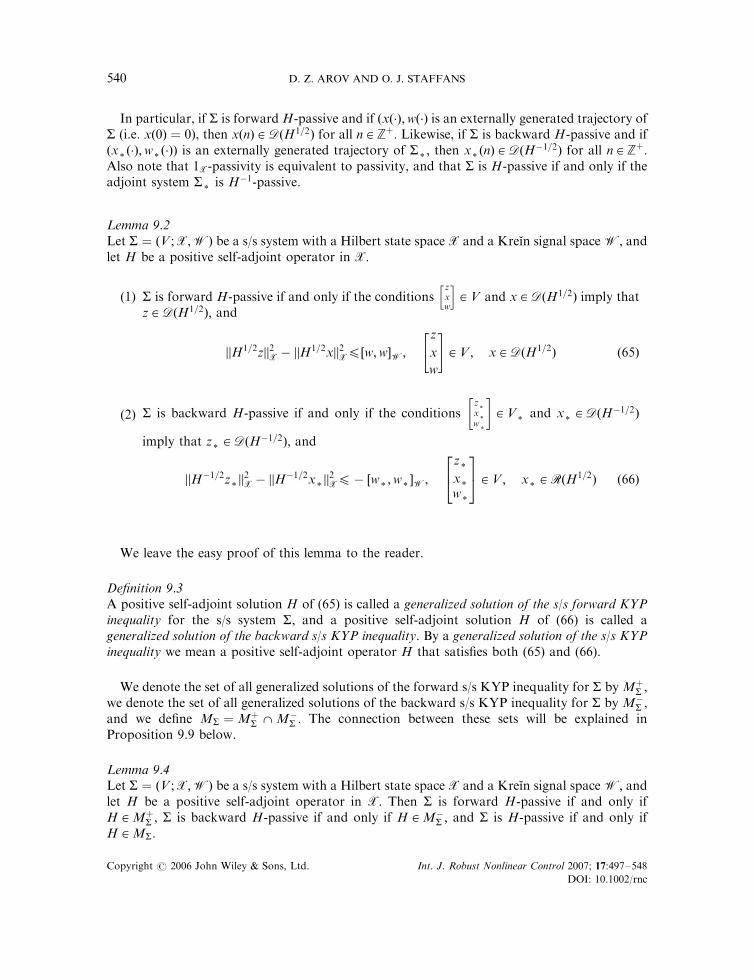
In particular, if S is forward H-passive and if ðxð�Þ;wð�Þ is an externally generated trajectory ofS (i.e. xð0Þ ¼ 0), then xðnÞ 2 DðH1=2Þ for all n 2 Zþ: Likewise, if S is backward H-passive and ifðx

*ð�Þ;w

*ð�ÞÞ is an externally generated trajectory of S

*; then x

*ðnÞ 2 DðH�1=2Þ for all n 2 Zþ:

Also note that 1X-passivity is equivalent to passivity, and that S is H-passive if and only if theadjoint system S

*is H�1-passive.

Lemma 9.2Let S ¼ ðV ;X;WÞ be a s/s system with a Hilbert state space X and a Kreın signal space W; andlet H be a positive self-adjoint operator in X:

(1) S is forward H-passive if and only if the conditionszxw

h i2 V and x 2 DðH1=2Þ imply that

z 2 DðH1=2Þ; and

jjH1=2zjj2X � jjH1=2xjj2X4½w;w�W;

z

x

w

" #2 V ; x 2 DðH1=2Þ ð65Þ

(2) S is backward H-passive if and only if the conditionsz*

x*

w*

� �2 V

*and x

*2 DðH�1=2Þ

imply that z*2 DðH�1=2Þ; and

jjH�1=2z*jj2X � jjH

�1=2x*jj2X4� ½w*

;w*�W;

z*

x*

w*

24

35 2 V ; x

*2 RðH1=2Þ ð66Þ

We leave the easy proof of this lemma to the reader.

Definition 9.3A positive self-adjoint solution H of (65) is called a generalized solution of the s/s forward KYPinequality for the s/s system S; and a positive self-adjoint solution H of (66) is called ageneralized solution of the backward s/s KYP inequality. By a generalized solution of the s/s KYPinequality we mean a positive self-adjoint operator H that satisfies both (65) and (66).

We denote the set of all generalized solutions of the forward s/s KYP inequality for S by MþS ;

we denote the set of all generalized solutions of the backward s/s KYP inequality for S by M�S ;

and we define MS ¼MþS \M�

S : The connection between these sets will be explained inProposition 9.9 below.

Lemma 9.4Let S ¼ ðV ;X;WÞ be a s/s system with a Hilbert state space X and a Kreın signal space W; andlet H be a positive self-adjoint operator in X: Then S is forward H-passive if and only ifH 2Mþ

S ; S is backward H-passive if and only if H 2M�S ; and S is H-passive if and only if

H 2MS:



DOI: 10.1002/rnc

ProofThis follows immediately from Lemma 9.2 and Definition 9.3. &

Proposition 9.5The behaviour of an H-passive system is passive.

ProofThe H-passivity of a s/s system S means that it is both forward and backward H-passive. Itfollows from (65) that the zero section Wð0Þ of the behaviour W of S is non-negative in W; andit follows from (66) that the zero section W

*ð0Þ of the adjoint behaviour W

*induced by S

*is

non-negative in W*: We recall from Proposition 4.4 that W

*ð0Þ ¼Wð0Þh?i; hence Wð0Þ½?� ¼

IW*ð0Þ is non-positive in W: By part (5) of Proposition 2.2, Wð0Þ is maximal non-negative in

W: By iterating (63) (starting with n ¼ 0 and xð0Þ ¼ 0) we find that W also has property (1) inDefinition 8.1. Thus, W is passive. &

Theorem 9.12 given below is a partial converse to Proposition 9.5.The above KYP inequalities can be reformulated by using different representations of S

(driving variable, output nulling, or i/s/o). For example, suppose that W has an orthogonaladmissible decomposition W ¼ �Y½ ’þ�U; where Y and U are Kreın spaces in the inner productinherited from W (this is a fundamental decomposition if Y and U are Hilbert spaces). Wedenote the corresponding i/s/o representation of S by Si=s=o ¼

AC

BD

� �;X;Y;U

� �: In terms of this

representation, H 2MþS if and only if

ADðH1=2Þ � DðH1=2Þ; BU� DðH1=2Þ ð67Þ

and

jjH1=2ðAxþ BuÞjj2X � jjH1=2xjj2X4½u; u�U

� ½CxþDu;CxþDu�Y; x 2 DðH1=2Þ; u 2 U ð68Þ

By the same argument combined with Proposition 4.11, H 2M�S if and only if

AnRðH1=2Þ � RðH1=2Þ; CnY� RðH1=2Þ ð69Þ

and

jjH�1=2ðAnx*þ Cny

*Þjj2X � jjH

�1=2x*jj2X4½y*

; y*�Y

� ½Bnx*þDny

*;Cnx

*þDny

*�U; x

*2 RðH1=2Þ; y

*2 Y ð70Þ

Thus, the set of positive self-adjoint solutions of (67)–(68) is the same as the set MþS of positive

self-adjoint solutions of (65), and the set of positive self-adjoint solutions of (69)–(70) is the same asthe set M�

S of positive self-adjoint solutions of (66). In the case where H is bounded the condition(67) holds automatically, and condition (68) may be rewritten as inequality (12) in the Kreınspace X½ ’þ�U:

More generally, it is possible to study the solutions H of (67)–(68) and (69)–(70)corresponding to an arbitrary i/s/o system Si=s=o ¼

AC

BD

� �;X;U;Y

� �without any reference to

an underlying s/s system. Here we allow Y and U to be Kreın spaces. In this case, we refer to(67)–(68) and (69)–(70) as the forward, respectively, backward, generalized transmission KYPinequalities. We call Si=s=o forward or backward H-passive if H is a generalized solution of the



DOI: 10.1002/rnc

forward or backward transmission KYP inequality, and we call Si=s=o H-passive if it is bothforward and backward H-passive. When Y and U are Hilbert spaces we replace the word‘transmission’ by ‘scattering’.

We denote the set of all generalized solutions of the forward transmission (or scattering) KYPinequality for Si=s=o by Mþ

Si=s=o; we denote the set of all generalized solutions of the backward

transmission KYP inequality for Si=s=o by M�Si=s=o

; and we define MSi=s=o¼Mþ

Si=s=o\M�

Si=s=o:

The above discussion may be summarized as follows.

Proposition 9.6Let S ¼ ðV ;X;WÞ be a s/s signal system which has an admissible orthogonal decompositionW ¼ �Y½ ’þ�U of the signal space. Let Si=s=o ¼

AC

BD

� �;X;U;Y

� �be the corresponding

transmission representation of S: Then the following claims are true:

(1) S is forward H-passive if and only if Si=s=o is forward H-passive, i.e. MþS ¼Mþ

Si=s=o:

(2) S is backward H-passive if and only if Si=s=o is backward H-passive, i.e. M�S ¼M�

Si=s=o:

(3) S is H-passive if and only if Si=s=o is H-passive, i.e. MS ¼MSi=s=o:

Thus, in particular, the sets MþSi=s=o

; M�Si=s=o

; and MSi=s=oare independent of the particular

orthogonal decomposition W ¼ �Y½ ’þ�U:

As our next proposition shows, if the decomposition W ¼ �Y½ ’þ�U is fundamental, so thatSi=s=o is a scattering representation of S; then forward and backward H-passivity are equivalent,so that in this case Mþ

S ¼M�S ¼MS: This was first proved in a i/s/o setting in Reference [14].

Proposition 9.7Let S ¼ ðV ;X;WÞ be a s/s signal system which has an admissible fundamental decompositionW ¼ �Y½ ’þ�U of the signal space. Then the following claims are equivalent:

(1) S is forward H-passive,(2) S is backward H-passive,(3) S is H-passive.

ProofLet Si=s=o ¼

AC

BD

� �;X;U;Y

� �be the scattering representation of S corresponding to the

decomposition W ¼ �Y½ ’þ�U: Then, by Proposition 9.6, S is forward H-passive if and only ifSi=s=o is forwardH-passive. By Reference [24, Proposition 4.6], Si=s=o is forwardH-passive if andonly if it is backward H-passive. Thus, (1) and (2) are equivalent. &

Theorem 9.8Let the s/s system S ¼ ðV ;X;YÞ be forward H-passive. Then the following conditions areequivalent:

(1) S is H-passive;(2) At least one fundamental decomposition W ¼ �Y½ ’þ�U of W is an admissible input/

output decomposition for S:(3) The zero section Wð0Þ of the behaviour W of S is a maximal non-negative subspace of

W:(4) The behaviour W of S is passive.



DOI: 10.1002/rnc

If these conditions hold, then every fundamental decomposition W ¼ �Y½ ’þ�U of W isadmissible.

ProofBy Proposition 9.5, (1) ) (4). Trivially, (4) ) (3), and by Corollary 5.9, (3) ) (1). ByProposition 8.5, (4) ) (1), and by Proposition 9.7, (2) ) (1). &

Proposition 9.9If both Mþ

S and M�S are non-empty, then MS is non-empty as well, and Mþ

S ¼M�S ¼MS:

ProofLetH 2Mþ

S andH1 2M�S : It follows from (65) that the zero section Wð0Þ of the behaviour W of

S is non-negative on W; and it follows from (66) with H replaced by H1 that the zero sectionW

*ð0Þ of the adjoint behaviour W

*induced by S

*is non-negative in W

*: Continuing in the

same way as we did in the proof of Proposition 9.5 we find that Wð0Þ is maximal non-negative inW: By Theorem 9.8, H 2MS: Thus, M

þS �M�

S : The same argument applied to the adjointsystem shows that also M�

S �MþS : &

Remark 9.10It is possible that one of the two sets Mþ

S and M�S is empty and the other non-empty. This is

true, for example, in Example 5.5, where MþS=| (it contains the identity) but M�

S ¼ | (it mustbe empty, since otherwise the system would be passive).

Proposition 9.11Let S ¼ ðV ;X;WÞ be a minimal s/s system with Hilbert state space X and Kreın signal space W:

(1) If S is H-passive for some H; then S is pseudo-similar to a unique passive systemSH ¼ ðVH ;X;WÞ with pseudo-similarity operator H1=2:

(2) Conversely, if S is pseudo-similar to a passive system S1 ¼ ðV1;X1;WÞ with similarityoperator Q; then S is H-passive with H ¼ QnQ; and S1 is unitarily similar to the systemSH in assertion (1).

ProofProof of (1): Let W ¼ �Y½ ’þ�U be a fundamental decomposition of W: By Proposition 9.7,this decomposition is admissible for S: Let Si=s=o ¼

AC

BD

� �;X;U;Y

� �be the corresponding

scattering representation of S: By Proposition 9.6, Si=s=o is H-passive. According toReference [14, Proposition 4.2], there exists a (unique) scattering passive i/s/o system

SHi=s=o ¼

AH

CH

BH

DH

h i;X;U;Y

� such that Si=s=o is pseudo-similar to SH

i=s=o with similarity operator

H1=2 (here AH is the closure of H1=2AH�1=2; CH is the closure of CH1=2; BH ¼ H1=2B; andDH ¼ D). Let SH ¼ ðVH ;X;WÞ be the corresponding s/s system. Then S is pseudo-similar toSH with pseudo-similarity operator H1=2: The uniqueness of SH is immediate: the system SH isuniquely determined by its trajectories, and the trajectories of SH are determined uniquely bythe trajectories of S and the pseudo-similarity H1=2:

Proof of (2): Let H ¼ QnQ: Then H is a positive self-adjoint operator in X withDðH1=2Þ ¼ DðQÞ; and Q has a polar decomposition Q ¼ UH1=2; where U is a unitary operator



DOI: 10.1002/rnc

mapping X onto X1 (see, e.g. Reference [45, p. 334]). Let VH ¼U�1zU�1xw

� �� zxw

h i2 V1

� : Then S1 is

unitarily similar to the minimal passive system SH ¼ ðVH ;X;WÞ; and the trajectories of SH areof the form ðU�1x1ð�Þ;wð�ÞÞ where ðx1ð�Þ;wð�ÞÞ is a trajectory of S1:Moreover, the operator H1=2

is a pseudo-similarity between S and SH : The passivity of SH now implies that S is H-passive. &

Theorem 9.12Let S ¼ ðV ;X;WÞ be a minimal s/s system with Hilbert state space X and Kreın signal spaceW: If the behaviour of S is passive, there exists a positive self-adjoint operator H with respect towhich S is H-passive, or equivalently, S is pseudo-similar to a passive system SH ¼ ðVH ;X;WÞwith pseudo-similarity operator H1=2: Moreover, it is possible to choose H in such a way thatSH is minimal, or equivalently,

H1=2R1 ¼ X; H�1=2R*1 ¼ X ð71Þ

where

R1 ¼[1n¼1

fxðnÞjðxð�Þ;wð�ÞÞ is an externally generated trajectory of Sgzzz

and R*1 is the corresponding subspace for S

*:

ProofBy Proposition 8.9, there exists minimal passive s/s system S1 ¼ ðV1;X1;WÞ which realizes thesame behaviour W as S: According to Proposition 3.3, the systems S and S1 are pseudo-similar.By assertion (2) of Proposition 9.11, S is H-passive where H ¼ QnQ; and H1=2 is a pseudo-similarity operator between S and SH : Thus, for any trajectory ðxð�Þ;wð�ÞÞ of S withxð0Þ 2 DðH1=2Þ we have xðnÞ 2 DðH1=2Þ for all n 2 Zþ; and ðH1=2xð�Þ;wð�ÞÞ is a trajectory of S:The converse is also true: for any trajectory ðxHð�Þ;wð�ÞÞ of SH with xHð0Þ 2 RðH1=2Þ we havexHðnÞ 2 RðH1=2Þ for all n 2 Zþ; and ðH�1=2xHð�Þ;wð�ÞÞ is a trajectory of S: This connection holds,in particular, for all externally generated trajectories (since xð0Þ ¼ 0 and xHð0Þ ¼ 0). Thisimplies that R1H ¼ H1=2R1; where R1H is the analogue of R1 for SH : The controllability ofSH implies thatH1=2R1 ¼ R1H ¼ X: By applying the same argument to the dual system we getH�1=2R

*1 ¼ X (recall that, by Theorem 4.13, H1=2 is a similarity between S*and ðSHÞ

*). &

It is possible to compare two generalized positive self-adjoint solutions of the KYP inequalityto each other by using the standard partial ordering of non-negative self-adjoint operators,which is defined as follows (see Reference [14] for details). If H1 and H2 are two non-negativeself-adjoint operators on the Hilbert space X; then we write H1%H2 whenever DðH1=2

2 Þ �DðH1=2

1 Þ and jjH1=21 xjj4jjH1=2

2 xjj for all x 2 DðH1=22 Þ: For bounded non-negative operators H1 and

H2 with DðH2Þ ¼ DðH1Þ ¼ X this ordering coincides with the standard ordering of boundedself-adjoint operators on X:

zzzThus, R1 consists of all those states of S that can be reached in some finite time, starting from the zero state.



DOI: 10.1002/rnc

Theorem 9.13Let S be a minimal s/s system with a passive behaviour, and let Mmin

S be the set of all solutionsof the KYP inequality for S that satisfy (71). Then Mmin

S is non-empty, and there exist uniqueH

82Mmin

S and H*2MminS such that

H84H4H�; H 2Mmin

S

ProofBy Theorem 9.12, the set Mmin

S is non-empty. Let W ¼ �Y½ ’þ�U be a fundamentaldecomposition of W: By Proposition 8.5, this decomposition is admissible for S: Let Si=s=o

be the corresponding scattering representation of S: Then, by Proposition 9.6, MS ¼MSi=s=o:

The existence of a minimal solution H8and a maximal solution H

8in Mmin

S now follows fromReference [14, Theorem 5.11 and Proposition 5.15]. &

Remark 9.14Above we studied the set Hmin

S by reducing the problem to the corresponding problem for i/s/osystems Si=s=o and scattering supply rate jðy; uÞ ¼ jjujj2U � jjyjj

2Y; which was solved in Reference

[14]. This reduction was based on the following facts:

(1) A decomposition W ¼ �Y ’þU is fundamental if and only if the inner product ½�; ��W inW induces the scattering supply rate jðy; uÞ ¼ �jjyjj2Y þ jjujj

2U on Y

U

� �; where jjyjj2Y ¼

�½y; y�W50 and jjujj2U ¼ ½u; u�W50 for all yu

� �2 Y

U

� �;

(2) every fundamental decomposition of W is admissible for an H-passive system S withKreın signal space W;

(3) if Si=s=o is a scattering representation of a s/s system S; then MþS ¼M�

S ¼MS; and thisset coincides with the corresponding sets for Si=s=o; i.e. M

þSi=s=o¼M�

Si=s=o¼MSi=s=o

¼MS:If, in addition, S is minimal, then the same statement remains true for Mmin

S :

This approach is not restricted to i/s/o systems with a scattering supply rate. The same argumentapplies to an arbitrary i/s/o system Si=s=o ¼

AC

BD

� �;X;U;Y

� �with Hilbert input and output

spacesU andY and with an arbitrary supply rate jðy; uÞ as long as this supply rate defines a Kreın

space inner product in the signal space W ¼ YU

� �: Each such supply rate has a representation of the

form jðy; uÞ ¼ yu

� �; J y

u

� �� YU

for some self-adjoint operator J ¼ J11J21

J12J22

h i2 BðYUÞ with a

bounded inverse. The decompositionW ¼ Y ’þU is orthogonal if and only if J is block diagonal, i.e.J12 ¼ 0 and J21 ¼ 0: In the case of a bounded operator H the (forward) KYP inequality forSi=s=o is given by

AnHA�H � CnJ11C AnHB� CnJ12 � CnJ11D

BnHA� J21C �DnJ11C BnHB�DnJ12 � J21D�DnJ11D� J22

" #40 ð72Þ

and MþSi=s=o

consists of generalized solutions of this inequality. The adjoint supply rate j*ðy; uÞ

which is applied to the adjoint i/s/o system Sn

i=s=o ¼An

Bn

Cn

Dn

h i;X;Y;U

� is given by

j*ðy; uÞ ¼ � y

u

� �; J�1 y

u

� �� YU

; and M�Si=s=o

consists of the inverses of all generalized solutions of

the KYP inequality for Sn

i=s=o: The system Si=s=o can be interpreted as an i/s/o representation of a



DOI: 10.1002/rnc

s/s system S with the signal space W ¼ YU

� �with Kreın space inner product y

u

� �; y0

u0

h ih iW¼

yu

� �; J y0

u0

h i� YU

for all yu

� �; y

y0

h iuu0

� �2 Y

U

� �; and with this interpretation Mþ

S ¼MþSi=s=o

and M�S ¼

M�Si=s=o

: Property (3) above is still valid in the weaker form presented in Proposition 9.9.

It is also possible to proceed in the opposite direction, and to consider the H-passive s/ssystem S to be the primary object, from which we can construct various H-passive i/s/o systemswith different supply rates. If W ¼ Y ’þU is an admissible decomposition for S; then the

corresponding i/s/o system Si=s=o is H-passive with respect to the supply rate on YU

� �inherited

from the inner product ½�; ��W:}}} Thus, in the family of i/s/o systems Si=s=o ¼

AC

BD

� �;X;U;Y

� �that we get from S by varying the decomposition W ¼ Y ’þU the coefficients A

CBD

� �vary, and so

do the supply rates jðy; uÞ; but the set of solutions MþSi=s=o

of the generalized KYP inequality (72)

stays the same. The same comment applies to the sets M�Si=s=o

and MSi=s=o; too.

ACKNOWLEDGEMENTS

Damir Z. Arov thanks Abo Akademi for its hospitality and the Academy of Finland for its financialsupport during his visits to Abo in 2003–2005. He also gratefully acknowledges the partial financialsupport by the joint grant UM1-2567-OD-03 from the U.S. Civilian Research and DevelopmentFoundation (CRDF) and the Ukrainian Government. Olof J. Staffans gratefully acknowledges thefinancial support by grant 203991 from the Academy of Finland.

REFERENCES

1. Arov DZ, Yakubovich VA. Conditions for the semiboundedness of quadratic functionals over Hardy spaces.Vestnik Leningradskogo Universiteta Matematika, Mekhanika, Astronomiya 1982; 1(vyp):11–18, 133.

2. Arov DZ, Staffans OJ. The infinite-dimensional continuous time Kalman–Yakubovich–Popov inequality. OperatorTheory: Advances and Applications 2006; 28.

3. Arov DZ, Staffans OJ. State/signal linear time-invariant systems theory. Part I: Discrete time systems. The StateSpace Method, Generalizations and Applications. Basel, Boston, Berlin (Operator Theory: Advances and Applications,vol. 161. Birkhauser: Basel, 2005; 115–177).

4. Petersen IR, Anderson BDO, Jonckheere EA. A first principles solution to the non-singular H1 control problem.International Journal of Robust and Nonlinear Control 1991; 1:171–185.

5. Ionescu V, Weiss M. Continuous and discrete-time Riccati theory: a Popov-function approach. Linear Algebra andits Applications 1993; 193:173–209.

6. Lancaster P, Rodman L. Algebraic Riccati Equations. Oxford Science Publications, The Clarendon Press, OxfordUniversity Press: New York, 1995.

7. Kalman RE. Lyapunov functions for the problem of Lur’e in automatic control. Proceedings of the NationalAcademy of Sciences 1963; 49:201–205.

8. Popov V-M. Hyperstability of Control Systems. Editura Academiei: Bucharest, 1973 (translated from the Romanianby Radu Georgescu, Die Grundlehren der mathematischen Wissenschaften, Band 204).

9. Yakubovich VA. The solution of some matrix inequalities encountered in automatic control theory. DokladyAkademii Nauk SSSR 1962; 143:1304–1307.

10. Yakubovich VA. The frequency theorem for the case in which the state space and the control space are Hilbertspaces, and its application in certain problems in the synthesis of optimal control. I. Sibirskii MatematicheskiiZhurnal 1974; 15:639–668, 703 (translation in Siberian Mathematical Journal 1974; 15:457–476).

}}}The transmission supply rate jðy; uÞ ¼ �½y; y�Y þ ½u; u�U corresponds to an orthogonal admissible decomposition W ¼�Y½ ’þ�U of the signal space W; and this case is discussed in Proposition 9.6.



DOI: 10.1002/rnc

11. Yakubovich VA. The frequency theorem for the case in which the state space and the control space are Hilbertspaces, and its application in certain problems in the synthesis of optimal control. II. Sibirskii MatematicheskiiZhurnal 1975; 16(5):1081–1102, 1132 (translation in Siberian Mathematical Journal 1974; 16:828–845).

12. Lihtarnikov AL, Yakubovich VA. A frequency theorem for equations of evolution type. Sibirskii MatematicheskiiZhurnal 1976; 17(5):1069–1085, 1198 (translation in Siberian Mathematical Journal 1976; 17:790–803).

13. Pandolfi L. The Kalman–Yakubovich–Popov theorem for stabilizable hyperbolic boundary control systems. IntegralEquations Operator Theory 1999; 34(4):478–493.

14. Arov DZ, Kaashoek MA, Pik DR. The Kalman–Yakubovich–Popov inequality and infinite dimensional discretetime dissipative systems. Journal of Operator Theory 2006; 55(2):393–438.

15. Willems JC. Dissipative dynamical systems. Part I: general theory. Archiv for Rational Mechanics and Analysis 1972;45:321–351.

16. Willems JC. Dissipative dynamical systems. Part II: linear systems with quadratic supply rates. Archiv for RationalMechanics and Analysis 1972; 45:352–393.

17. Azizov TYa, Iokhvidov IS. Linear Operators in Spaces with an Indefinite Metric. Wiley: New York, London, 1989.18. Bognar J. Indefinite inner product spaces. Ergebnisse der Mathematik und ihrer Grenzgebiete, vol. 78. Springer:

Berlin, Heidelberg, NY, 1974.19. Dritschel MA, Rovnyak J. Operators on indefinite inner product spaces. In Lectures on Operator Theory and its

Applications, Waterloo, ON, 1994. Fields Institute Monographs, vol. 3. American Mathematical Society,Providence, RI, U.S.A. 1996; 141–232.

20. Malinen J, Staffans OJ, Weiss G. When is a linear system conservative? Quarterly of Applied Mathematics 2006;64:61–91.

21. Staffans OJ. J-energy preserving well-posed linear systems. International Journal of Applied Mathematics andComputer Science 2001; 11:1361–1378.

22. Staffans OJ. Passive and conservative infinite-dimensional impedance and scattering systems (from a personal pointof view). Mathematical Systems Theory in Biology, Communication, Computation, and Finance (New York), IMAVolumes in Mathematics and its Applications, vol. 134. Springer: Berlin, 2002; 375–414.

23. Staffans OJ. Well-Posed Linear Systems. Cambridge University Press: Cambridge, New York, 2005.24. Weiss G, Staffans OJ, Tucsnak M. Well-posed linear systems}a survey with emphasis on conservative systems.

International Journal of Applied Mathematics and Computer Science 2001; 11:7–34.25. Alpay D, Dijksma A, Rovnyak J, de Snoo H. Schur functions, operator colligations, and reproducing kernel Hilbert

spaces. Operator Theory: Advances and Applications, vol. 96. Birkhauser-Verlag: Basel, Boston, Berlin, 1997.26. Arov DZ. Scattering theory with dissipation of energy. Doklady Akademii Nauk SSSR 1974; 216:713–716

(translation in Soviet Mathematics Doklady 1974; 15:848–854).27. Arov DZ. Stable dissipative linear stationary dynamical scattering systems. Journal of Operator Theory 1979; 1:

95–126 (translation in Reference [41]).28. Arov DZ, Kaashoek MA, Pik DR. Minimal and optimal linear discrete time-invariant dissipative scattering systems.

Integral Equations Operator Theory 1997; 29:127–154.29. Arov DZ, Rovnyak J, Saprikin SM. Linear passive stationary scattering systems with Pontryagin state spaces.

Manuscript, 2004.30. Ball JA, Cohen N. De Branges–Rovnyak operator models and systems theory: a survey. Topics in Matrix and

Operator Theory. Basel, Boston, Berlin, 1991 (Operator Theory: Advances and Applications, vol. 50. Birkhauser:Basel, 1991; 93–136).

31. de Branges L, Rovnyak J. Canonical models in quantum scattering theory. Perturbation theory and its applicationsin quantum mechanics. Proceedings of an Advanced Seminar, Calvin H (ed.), Mathematics Research CenterU.S. Army, Theoretical Chemistry Institute, University of Wisconsin, Madison, Wis., 1965. Wiley: New York,1966; 295–392.

32. de Branges L, Rovnyak J. Square Summable Power Series. Holt, Rinehart and Winston: New York, 1966.33. Arov DZ, Nudelman MA. Passive linear stationary dynamical scattering systems with continuous time. Integral

Equations Operator Theory 1996; 24:1–45.34. Ball JA, Staffans OJ. Conservative state–space realizations of dissipative system behaviors. Integral Equations

Operator Theory 2006; 54:151–213.35. Nudelman MA. Optimal passive systems and semiboundedness of quadratic functionals (in Russian). Sibirskii

Matematicheskii Zhurnal 1992; 33:78–86 (translation in Siberian Journal of Mathematics 1992; 33:62–69).36. Staffans OJ. Passive and conservative continuous-time impedance and scattering systems. Part I: Well-posed

systems. Mathematics of Control, Signals, and Systems 2002; 15:291–315.37. Staffans OJ. Stabilization by collocated feedback. Directions in Mathematical Systems Theory and Optimization

(New York), Lecture Notes in Control and Information Sciences, vol. 286. Springer: Berlin, 2002; 261–278.38. Tucsnak M, Weiss G. How to get a conservative well-posed linear system out of thin air. Part II. Controllability and

stability. SIAM Journal on Control Optimization 2003; 42:907–935.39. Weiss G, Tucsnak M. How to get a conservative well-posed linear system out of thin air. I. Well-posedness and

energy balance. ESAIM Control Optimization and Calculus of Variations 2003; 9:247–274.



DOI: 10.1002/rnc

40. Arov DZ. Passive linear stationary dynamic systems. Sibirskii Matematicheskii Zhurnal 1979; 20:211–228(translation in Siberian Mathematical Journal 1979; 20:149–162).

41. Arov DZ. Stable dissipative linear stationary dynamical scattering systems. Interpolation Theory, Systems Theory,and Related Topics, The Harry Dym Anniversary Volume. Basel, Boston, Berlin (Operator Theory: Advances andApplications, vol. 134. Birkhauser: Basel, 2002, 99–136) (translation of Reference [27]).

42. Arov DZ, Nudelman MA. Criterion of unitary similarity of minimal passive scattering systems with a given transferfunction. Ukrainian Mathematical Journal 2000; 52:161–172.

43. Arov DZ, Nudelman MA. Tests for the similarity of all minimal passive realizations of a fixed transfer function(scattering or resistance matrix). Sbornik Mathematics 2002; 193:791–810.

44. Sz.-Nagy B, Foias- C. Harmonic Analysis of Operators on Hilbert Space. North-Holland: Amsterdam, London, 1970.45. Kato T. Perturbation Theory for Linear Operators. Springer: Berlin, Heidelberg, NY, 1980.



DOI: 10.1002/rnc

state/signal linear time-invariant systems theory: passive discrete time systems

Documents