states for interconnected power system de was proposed in ... · supervisory control and data...

IET Generation, Transmission & Distribution

Research Article

Hierarchical parallel dynamic estimator ofstates for interconnected power system

ISSN 1751-8687Received on 1st November 2017Revised 24th January 2018Accepted on 15th February 2018E-First on 14th March 2018doi: 10.1049/iet-gtd.2017.1733www.ietdl.org

Sreenath Jayakumar Geetha1 , Saikat Chakrabarti1, Ketan Rajawat11Department of Electrical Engineering, Indian Institute of Technology Kanpur, Kanpur, UP 208016, India

E-mail: [email protected]

Abstract: Real-time visualisation of large power systems, by tracking the system states, is a challenging task as it involvesprocessing a large measurement set to obtain the system states. This study proposes a hierarchical parallel dynamic estimationalgorithm to estimate the states of a large-scale interconnected power system. The power system is decomposed into smallersubsystems, which is processed in parallel to obtain a reduced order state estimate. This information is then transmitted to thecentral processor, which collates the individual reduced order estimates to obtain the global estimates. Each processor usesstate matrix of smaller dimension, thereby reducing the computational burden. The low-level processors utilise only a fraction ofthe global measurements in the proposed approach, and there is no need for any information exchange from the centralprocessor to the low level processors, which helps in reducing the communication requirements. Moreover, detection ofanomalies can also be carried out at the local processors without the need for any separate bad data detection at the centralprocessor. IEEE 30- and 118-bus systems are used as test beds to study the proposed approach.

1 IntroductionState estimator (SE) in a power system determines the systemstates at all the buses [1, 2], and it is the primary tool used tomonitor, protect, and control the operation of a power system.Generally, a weighted least squares (WLS)-based SE algorithm isutilised by system operators to obtain a snapshot of the system [3].This approach is inherently static in nature, as it does not considerthe correlation between the present and the previous states, whileprocessing the latest set of measurements. The conventionalmeasurement set typically consists of real and reactive powerinjection and flow measurements, voltage magnitudemeasurements, and current magnitude measurements. Thesupervisory control and data acquisition (SCADA) system collectsthe conventional measurements, which are then processed by theSE to obtain the most likely states of the power system.

Power system loads vary continuously over a day following acertain load pattern. These load changes and the subsequentgeneration adjustments are characteristically slow and smoothtransitions. Hence, the power system can be considered to be a timeevolving quasi-static system. However, the static SE does notconsider any past history of the state variables and neglectstransition of the system states altogether. The information extractedfrom the previous states can be utilised to obtain a predictivedatabase, which can further improve the bad data detection analysisand security analysis functions. The predicted information can alsobe used as pseudo-measurements to improve data redundancy inmetering applications that encounter low data redundancy issues[4]. Hence, to determine the behaviour of the power system withtime, utilisation of an algorithm to estimate the system statesdynamically is thoroughly justified [5]. Estimators which considerthe temporal correlation between the states are commonly referredto as dynamic state estimators. However, this may lead toambiguity, as dynamic states normally relate to time varying statessuch as rotor angle, flux linkages in power systems [6]. This paperuses the term dynamic estimator (DE) for power system states torefer to the estimator which considers the time evolution of thepower system states and estimates the states dynamically.

Kalman filters [7] can be employed to estimate the states in DE.However, the standard Kalman filter can be applied only on linearsystems. The conventional measurement set of the power systeminclude real and reactive power injections and power flows, which

are non-linear functions of the states and the line parameters of thepower system. To address the non-linearities, extensions of thestandard Kalman filter, namely the extended Kalman filter (EKF)and the unscented Kalman filter, have been developed [5, 8].However, these techniques add to the computational complexity,and therefore, estimating the states of a very large power system toobtain a real time representation can be a very challenging task [9].

Parallel state estimation (PSE) algorithms were proposed toaddress the computational complexity issue arising in large-scalesystems [10]. In this approach, a large system is divided intosmaller subsystems, and are processed in parallel. The localestimates of each processor are then collectively combined at acentral processor to obtain the global estimates. A detailed reviewof various hierarchical algorithms is discussed in [10]. Apart fromreducing the computational burden, hierarchical algorithms alsohelp in improving the reliability of the estimator.

Several researchers have studied the solution of hierarchicalalgorithms considering different decomposition strategies,coordination schemes etc. as discussed in [10]. A two-levelestimator, which uses synchrophasor measurements at the centrallevel, was discussed in [11]. All these studies focus onimplementing the PSE in the static sense. However, very littleresearch has been carried out in implementing parallel DE forlarge-scale power systems. A hierarchical DE algorithm wasproposed in [12], which extends the hierarchical scheme proposedfor the static SE in [13]. The work in [14] considers thehierarchical DE problem by utilising an artificial neural network(ANN)-based load prediction algorithm. An agent-based multi-areaDE was proposed in [15]. These methods require transmitting theraw measurements directly to the central processor which increasesthe communication .requirements. A parallel programming methodto speed up the execution time of an EKF-based DE implementedon graphic processing unit is discussed in [16]. A distributed point-based Gaussian approximation filter to estimate the power systemstates dynamically is proposed in [17]. However, in this methodeach local processor considers the full state space model whichresults in higher communication and computational requirements.

The hierarchical parallel dynamic estimator (HPDE) algorithmproposed in this paper uses an interprocessor transformationmatrix-based method to process a subset of the global measurementvector in parallel at the low-level processors and obtains a stateestimation vector of reduced dimensionality. This information is

IET Gener. Transm. Distrib., 2018, Vol. 12 Iss. 10, pp. 2299-2306© The Institution of Engineering and Technology 2018

2299

then collated at a central processor using the same transformationmatrix in order to obtain the global estimates, as discussed in [18].The proposed approach results in globally optimal estimates if theglobal state vector can be decomposed into completely disjointpartitions. However, in power systems, as measurements belongingto one subsystem can affect the states of neighbouring subsystemsto which it is connected, creating disjoint reduced order statevectors may not be possible. An extended subsystem configuration,which will be discussed in detail in Section 3, can ensure sufficientmeasurement redundancy, and maintain acceptable quality of theestimates. Optimal solution for this case can be achieved usingbidirectional communication between the low-level processors andthe central processor. However, this would lead to increasedcommunication requirements and higher computation time. Thesub-optimality of the proposed approach should be viewed as anacceptable trade-off for reduced interprocessor communication andimproved system throughput.

The main contribution of this work is: (i) to develop a parallelDE using an interprocessor transformation matrix, for large-scalepower systems, by implementing a bank of low-dimensionalparallel DEs and a full-dimensional central DE to reduce thecomputational complexity inherent in a centralised estimator; (ii) toreduce the interprocessor communication requirements by limitingthe data transferred between the processors; and (iii) to avoidchecking for any bad data in the raw measurements at the centralprocessor by not transmitting any measurement directly to thecentral processor.

The algorithm operates such that there is no need to transmitany raw measurement to the central processor. Angle referencing iscarried out at the central processor using local estimates, asdiscussed in [19]. Since all the measurements are transmitted to thecentral processor, indirectly, estimates obtained centrally bycollating the local information do not lose in estimation accuracy.The reduced order local processing slackens the computationalburden that was shouldered by the monolithic central processor,thereby enhancing the reliability and robustness of the estimator.The effectiveness of the proposed method is tested using IEEE 30-and 118-bus systems. The results obtained are compared to anintegrated state estimator (ISE) algorithm [5].

This paper is organised as follows: Section 2 illustrates theextended Kalman and information filter algorithms for anintegrated power system, Section 3 introduces decomposing thepower system to extended subsystems, Section 4 describes theproposed HPDE algorithm, Section 5 discusses the implementationof the proposed algorithm on two test systems and analyses theresults, Section 6 discusses anomaly detection, and Section 7concludes the paper.

2 Integrated state estimatorIn an ISE for power system, all the collected measurements aresent to a central estimator which processes the measurements toobtain the global state vector. The integrated power system and themeasurement vector can be modelled [5], respectively, as

xk = Fk − 1xk − 1 + gk − 1 + Gk − 1qk − 1 ∀k = 1, …, n (1)

zk = h(xk) + rk (2)

where xk is the state vector, Fk − 1 is the state transition matrix, gk − 1

is the trend setting vector, qk − 1 is the white Gaussian noise vectorwith zero mean and covariance Qk − 1, n is the total number of time-steps, h is the vector of measurement functions, rk is the whiteGaussian error vector with zero mean and covariance Rk, Gk − 1 isthe noise model and is an identity matrix in this case

The measurement equation, (2), can be rewritten in linear form[7] as

Δzk = HΔxk + rk (3)

where Hk = ∂h/∂x is the measurement Jacobian matrix, Δxk andΔzk are the incremental state vector and the measurement deviationvector around the point of linearisation.

The most accepted and the widely used approach to determinethe state transition matrix, Fk, and the trend setting vector, gk, is theHolt's two-parameter linear exponential smoothing technique [5],as given below

Fk = αk(1 + βk)I (4)

gk = (1 + βk)(1 − αk)x̂k |k − 1 − βkak − 1 + (1 − βk)bk − 1 (5)

Here x̂k |k − 1 is the a priori estimate of the state vector at step k, ak − 1

and bk − 1 are the smoothed value of the time series and the estimateof the trend of the time series at time k − 1, respectively, and αk, βkare the parameters, whose values lie in the range of 0–1.

2.1 Kalman filter implementation

2.1.1 State prediction: Let x̂k − 1|k − 1 be the estimate of the statevector, and P^k − 1|k − 1 be the estimate of the error covariance matrixat step k − 1. Using these values, the a priori estimate of the statevector and the corresponding covariance matrix at step k arecalculated as

x~k |k − 1 = Fk − 1x̂k − 1|k − 1 + gk − 1 (6)

P~

k |k − 1 = Fk − 1P^

k − 1|k − 1Fk − 1T + Qk − 1 (7)

2.1.2 Innovation analysis: Once the new set of measurements atstep k, zk, is available, a data validation can be implemented usingthe normalised innovation vector, νk, to identify the presence ofanomalous data [4]. The innovation vector is defined as

νk = zk − h(x~k |k − 1) (8)

Once νk is obtained, the normalised innovations are calculated as

νkn(i) = νk(i)/ Yk(i, i) (9)

where Yk(i, i) is the standard deviation of the ith innovation, andis defined as

Yk = Rk + HkP~

k |k − 1HkT (10)

2.1.3 State update: After zk, is available, the a priori estimates isupdated to obtain the estimates, x̂k |k, and its correspondingcovariance matrix, P^k |k, by minimising the objective function givenas

J(x) = [z − h(x)]R−1[z − h(x)]T + [x − x~]P~−1[x − x~]T (11)

The time index, k, was removed from the above equation to make itsimpler. The value of x, which minimises the objective function,gives the best estimate of the system state at time k. Choosing the apriori estimate, x~k |k − 1, as the initial value and performing only asingle iteration, the estimate of the state vector at step k is obtainedas [5]

x̂k |k = x~k |k − 1 + Kk(zk − h(x~k |k − 1)) (12)

where Kk, the Kalman gain, is given as[7]

Kk = P~

k |k − 1HkT(HkP

~k |k − 1Hk

T + Rk)−1 (13)

The estimate of the state error covariance matrix is obtained as

P^k |k = (I − KkHk)P~

k |k − 1 (14)

2300 IET Gener. Transm. Distrib., 2018, Vol. 12 Iss. 10, pp. 2299-2306© The Institution of Engineering and Technology 2018

where I represents an identity matrix.

2.1.4 Residual analysis: The residual vector is defined as

ζk = zk − h(x̂k |k) (15)

Once ζk is obtained, the normalised residuals are calculated as

ζkn(i) = ζk(i)/ Ek(i, i) (16)

where Ek(i, i) is the standard deviation of the ith innovation, andis defined as

Ek = Rk + HkP~

k |kHkT (17)

2.2 Extended information filter implementation

Information filter is an alternate form of the Kalman filter thatpropagates the inverse of the error covariance matrix, P, known asthe information matrix. This form of Kalman filter helps in

simplifying the fusion of the distributed local estimates at a centralprocessor effectively. The state correction (12) and (14) can berewritten in the information filter form as [7]

P^k |k−1

x̂k |k = P~

k |k − 1−1 x~k |k − 1 + HkRk

−1z′k (18)

z′k = zk − h(x~k |k − 1) + Hkx~k |k − 1 (19)

P^k |k−1 = P

~k |k − 1−1 + HkRk

−1Hk (20)

3 Decomposition of large interconnected powersystemThe traditional SE utilises a centralised filter to process themeasurements, which can result in severe computational burdendue to the huge volume of data the filter has to handle. A PDEassuages this problem by dividing the huge power system networkinto relatively smaller subsystems. In this paper, it is assumed thatthe subsystem boundaries overlap partially to create an extendedsubsystem as shown in Fig. 1 [11, 19].

An extended subsystem includes all the internal buses and theboundary buses of the respective subsystem and all the boundarybuses of the neighbouring subsystems which is directly connectedto a boundary bus of the subsystem under consideration. Thisforms a partially overlapping extended subsystem, more commonlyreferred to as tie-line overlapping structure [10], where twoneighbouring areas share tie-lines and the corresponding boundarybuses. As illustrated in Fig. 1, the extended subsystem 1 includesbus 1-i1 and 1-i2, the internal buses of subsystem 1, bus 1-b1 and1-b2, the boundary buses of subsystem 1, and buses 2-b1 and 3-b1,the boundary buses of subsystem 2 and 3, respectively, to whichsubsystem 1 is connected through tie-lines. The extendedsubsystem configuration is best suited for angle referencing amongsubsystems, as discussed in [19], thereby prohibiting the need totransmit any raw measurements directly to the central processor.

The local processor of each of these extended subsystems thenprocesses the available measurements to obtain the best estimatesof the states belonging to that particular subsystem. The availablemeasurements, at a local processor, include all the internalmeasurements together with the power injections at the boundarybuses of the subsystem and the power flow in the tie-linesmeasured at the boundary bus side of the corresponding subsystem.The power injection measurements and the tie-line power flowmeasurements ensure the observability of boundary buses ofneighbouring subsystems to which the subsystem underconsideration is connected, thereby forming an extendedsubsystem. The estimates obtained by the local processor of eachsubsystem are then transmitted to the central estimator to obtain theglobal system estimate, as shown in Fig. 2. On the contrary, thecentralised estimator receives measurements from each subsystembefore processing them collectively to obtain the system states.

4 Hierarchical parallel dynamic estimatorThe integrated system in (1) can be partitioned into N extendedsubsystems. The superscript j is used to refer to the jth subsystemof the power system, where j = 1, …, N. The state vectorcorresponding to each subsystem, xk

j, can be related to the globalstate vector, xk, through the following transformation:

xkj = Dk

jxk (21)

where Dkj is the interprocessor transformation matrix of subsystem

j.The global measurement vector, zk, given in (2), is divided into

N sub-vectors, corresponding to each subsystem. The measurementmodel matrix, Hk, and the measurement noise vector, rk, are alsopartitioned into N sub-matrices and sub-vectors, respectively, asgiven below

Fig. 1 Illustration of an extended subsystem

Fig. 2 Hierarchical estimator, in which the estimates of each subsystemare communicated to the central level to obtain the global estimates


2301

zk = [(zk1)T(zk

2)T…(zkN)T]T (22)

Hk = [(Hk1)T(Hk

2)T…(HkN)T]T (23)

rk = [(rk1)T(rk

2)T…(rkN)T]T (24)

The partition Hkj is the jth row block of H and is of dimension

mj × n, where mj is the number of measurements to be processedby subsystem j and n is the number of states of the ISE.

Each subsystem has its own processor to estimate the local statevector using the measurements pertaining to that particularsubsystem. The local information is then communicated to thecentral processor, which collates the local information to calculatethe global estimates. In the proposed approach, there is nocommunication from the central processor to the low-levelprocessors, which help in reducing the communication overhead.The execution of each low-level processor is not dependent onneighbouring processors or the central processor. This allows eachsubsystem to process its measurements in parallel, therebyreducing the computation time. However, as all the measurementsrelated to a boundary bus are not available at the low-levelprocessors, this method is sub-optimal. A bidirectionalcommunication structure between low-level processors and centralprocessor can tackle this issue. However, this would lead toincreased communication requirements. Even though sub-optimal,the proposed method provides good estimates as a high degree ofredundancy can be ensured using the available local measurements.

From (1), the dynamical model of each individual subsystem isgiven as

xkj = Fk − 1

j xk − 1j + gk − 1

j + qk − 1j ∀k = 1, …, n (25)

It is assumed that each individual subsystem has its own localKalman filter that processes its own measurement set zk

j, which, inincremental form is given as

Δzkj = Ck

jΔxkj + rk

j (26)

where Ckj is the measurement Jacobian matrix of subsystem j.

Using (22)–(24), the measurement sub-vector of subsystem jcan be related to the global state vector, xk, as follows:

Δzkj = Hk

jΔxk + rkj (27)

Using the transformation (21), (26) can be rewritten as

Δzkj = Ck

jDkjΔxk + rk

j (28)

From (27) and (28), the measurement model partition, Hkj, and the

subsystem measurement model, Ckj, can be related as

Hkj = Ck

jDkj (29)

4.1 Low-level estimation

The state vector of subsystem j would contain all its interior statesand the states of the boundary buses of the adjacent subsystems, towhich it is connected. Any arbitrary bus can be chosen as theglobal slack bus. Each subsystem then executes its own Kalmanfilter to estimate the local states.

Step 1: State prediction: Let x̂k − 1|k − 1j be the estimate of the state

vector, and P^k − 1|k − 1j

be the estimate of the error covariance matrixat step k − 1. The a priori estimate of the state vector and thecorresponding covariance matrix at step k are calculated using thestate prediction equations given by (6) and (7) using the system andmeasurement model given by (25) and (26).

Step 2: State correction: Once the new set of measurements at stepk, zk

j, is available, the a priori estimates can be corrected to obtain

the estimates x̂k |kj and its corresponding covariance matrix P^k |k

j

using state correction (12)–(14).

The presence of bad data in the measurements processed by thelow-level processors can be detected by using a combination of thepredicted states and the filtered states. The predictive database ofthe DE helps in reducing the difficulties involved in detectinganomalies, while using a static SE [4]. This is discussed further inSection 6.

4.2 Communication to the central processor and anglereferencing

Transmitting the local estimates and covariances to the centralprocessor, let P^ j indicate the covariance matrix of the jthsubsystem at time k in simplified form. Similarly, P

~j, x̂ j, and x~ j are

used to represent the predicted covariance matrix, the estimatedstates, and the predicted states of subsystem j at time k,respectively. The central coordinator then performs angleadjustments using estimates of the boundary buses provided byeach subsystem, as discussed in [19]. The angle referencing is donebased on the following equation:

Δθ( j, b) = θ( j, b)G − θ( j, b)

L (30)

where G indicates the global reference, b is the bus number, θ( j, b)G is

the angle of the boundary bus b of the extended subsystem jestimated by the subsystem where the global slack bus lies, θ( j, b)

L isthe angle of the boundary bus b estimated by subsystem j, andΔθ( j, b) is the slack bus adjustment value used to adjust bus anglesof the subsystem j with respect to the global slack.

4.3 Information assimilation

Once the angle referencing has been completed, the centralprocessor moves on to assimilate the local information that hasbeen made available to it by the low-level processors, as discussedin [18].

Step 1: State prediction: The state predictions are carried out at thecentral processor based on the centralised Kalman filter (6) and (7),to obtain x~ and P

~.

Step 2: Parallel implementations for state correction: The centralprocessor involves continuous summation of the data. In theinformation filter form, the assimilation of the local estimates isgiven as

P^−1 = P

~−1 + ∑j = 1

NH j

TRj−1H j (31)

P^−1

x̂ = P~−1x~ + ∑

j = 1

NH j

TRj−1z′ j (32)

Substituting (29) into (31) and (32), we get

P^−1 = P

~−1 + ∑j = 1

NDj

T[C jTRj

−1C j]DjT (33)

P^−1

x̂ = P~−1x~ + ∑

j = 1

NDj

T[C jTRj

−1z′ j] (34)

Equations (33) and (34) can be rewritten using the local estimatesand the covariances as


P^−1 = P

~−1 + ∑j = 1

NDj

T(P^ j−1 − P

~j−1)Dj (35)

P^−1

x̂ = P~−1x~ + ∑

j = 1

NDj

T(P^ j−1

x̂ j − P~

j−1x~ j) (36)

From (31)–(36), it can be noticed that all the measurementsobtained at the low level processors are transmitted to the centralprocessor indirectly. There is no need to communicate thesubsystem topology to the central processor.

In the existing hierarchical estimators [11], raw measurementsare processed by the low-level processors as well as the centralprocessor, and hence there is a need to include bad data detectionalgorithm at both levels of the hierarchy. In the proposed HPDE,the local-level processors can use its predictive database along withthe filtered information to detect bad data in the measurements [4].The raw measurements are not transmitted to the central processor,which eliminates the need for a data debugger at the central level.

The advantages obtained using the proposed algorithm aresummarised below.

• Each local processor utilises only its own local measurements,and there is no information exchange from the central processorto the local processor, i.e. downwards in hierarchy, whichreduces the data exchange overhead.

• Each subsystem processes in parallel the availablemeasurements, thereby reducing the computational burden.

• There is no need to transmit any raw measurement to the centralprocessor, which helps in reducing the communicationrequirements.

• If any one of the local processor fails, the remaining subsystemswould have its own local estimates, leaving only a part of thelarger system unobserved.

• Using this approach, there is no need for individual subsystemsto exchange local topology information, which helps inpreserving sensitive internal information.

• The proposed method can be used for any measurementconfiguration, conventional only, SCADA only, or hybridmeasurement configuration.

• Since the central processor involves continuous summation toassimilate the local information, there is no need for the centralprocessor to wait till all the local information is made availableto it. As soon as a local information is available at the centralprocessor, it can start processing the information, which helps inreducing the total estimation time.

• There is no need for any separate bad data detection at thecentral processor, as none of the raw measurements aretransmitted to the central level.

5 Simulation casesThe HPDE, discussed in the previous section, was tested usingIEEE 30- and 118-bus systems, by dividing them into two [19] andnine [11] extended subsystems, respectively. The quasi-staticnature of the power system, i.e. the slow variation of the systemloads, is simulated by varying the loads at some of the busesrandomly within a range of ±10% of the base case value. Thegenerator outputs are also changed to meet the load changes. Thegenerations are varied based on their participation factors, which isset according to the ratio of their base case generations [20]. ANewton–Raphson load flow (NRLF) programme is run to obtainthe true power system states, by varying the generations and loads,as discussed above. For the purpose of simulation, themeasurements are generated by adding a random Gaussian noisewith zero mean and variance, ui

2, where ui is the standarduncertainty in the ith measurement. The standard uncertainties arecalculated using the maximum measurement uncertainties asspecified by the device manufacturers. It is assumed that allmeasurements except the phase angles are independent of eachother. So the error covariance matrix, R, would contain only thediagonal elements corresponding to these measurements [20].

The performance of the HPDE is evaluated by recording thedeviations in the estimated states from the true states, as shownbelow

η = 1S ∑

i = 1

N 1M ∑

k = 1

M(x̂k

i − xki)

2(37)

where η is the mean-squared error (MSE) in estimation, x̂krepresents the estimated state, xk is the true state, M is the numberof executions of the DE, and S is the total number of runs of theentire process, each considering M number of DE executions.

In order to initialise the Holt's technique as explained in [8], thefirst two samples of the state vectors are obtained using staticWLS. The elements of the measurement error covariance matrix,R, obtained from the maximum measurement uncertaintiesspecified by the device manufacturers, are kept constant for theentire simulation. The state estimation error covariance matrix, P,is initialised with its diagonal elements set to a very small value,namely 10−6. The diagonal elements of the matrix Q are also keptconstant at 10−6 for the entire process [8].

The proposed HPDE was implemented using MATLAB [21],and tested on IEEE 30- and 118-bus test systems [22]. To obtainthe predicted states, using Holt's method, the parameters α and βwere set to 0.9 and 0.1, respectively. For the purpose of anglereferencing, bus 1 of each system was considered to be thereference bus. The DE implemented in MATLAB was simulated ona computer using an Intel Core-i3 3.4 GHz processor and 4 GBRAM.

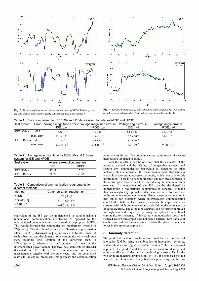
The simulation was performed for a total of 100 samples. Thesimulation was carried out under the assumption that the powersystem was in a quasi-static state. The loads at the various buses ofthe power system were varied within a small band to simulate thequasi-static behaviour of the system. The same measurement setwas used for both the ISE and the HPDE. The redundancy of themeasurement set is quantified as m/n, where m is the total numberof measurements and n is the total number of states. The chosenmeasurement configuration yields a redundancy of 1.76 and 1.82for the IEEE 30- and 118-bus systems, respectively, in the ISEconfiguration. For demonstration purpose, the values of the truestates and the estimated states for the HPDE are plotted for bothmagnitude and angle, for buses with the lowest estimationaccuracy, for IEEE 30- and 118-bus systems, as shown in Figs. 3and 4, respectively.

Table 1 compares the average of the mean-squared error and themaximum errors at all the buses for IEEE 30- and 118-bus testsystems for the ISE and HPDE. From Table 1, it can be observedthat the estimation accuracy of the proposed HPDE is comparableto the ISE. Although the proposed method is sub-optimal, due tosharing of the boundary bus states by various subsystems, theavailable local measurements ensure good redundancy and result inaccurate estimates. The sub-optimal results can affect the estimatesof other states, as there exists a correlation between the states.However, the Holt's method, used in this paper, assumes that thestate variables are uncorrelated and this assumption does not allowdegradation of the estimator performance [5].

Table 2 lists the execution time required to process onemeasurement set for the integrated SE and HPDE. In this paper, itis assumed that the central processor of the HPDE starts fusing thelocal estimates only after it has received information from all thesubsystems. However, in practical implementations, the centralprocessor can start fusing the local estimates as and when itreceives the information. The results given in Table 2, therefore,illustrate the worst case operation scenario of the proposed HPDE.

5.1 Communication requirements

Let the power system be decomposed into N subsystems. Eachsubsystem has to communicate a state vector and a covariancematrix to adjacent processors or the central processor depending onthe parallel architecture implemented. The HPDE proposed in thispaper requires a total of N(nj

2 + nj) elements to be communicated atevery time step. Here nj is number of states at subsystem j. An


2303

equivalent of the ISE can be implemented in parallel using abidirectional communication architecture as opposed to theunidirectional communication scheme used in the proposed HPDE.This would increase the communication requirement twofold to2N(nj

2 + nj). The distributed point-based Gaussian approximationfilter (DPGAF), discussed in [17], utilises a full-order model ateach subsystem and the elements to be communicated at each timestep, assuming one iteration at the consensus step, is2(N − 1)(n2 + n), where n is total number of states in theinterconnected power system. The two-level architectures (HDSE)discussed in [12, 14] involve communication of m rawmeasurements together with the state vector and the covariancematrix to the central processor. This increases the communication

requirements further. The communication requirements of variousmethods are tabulated in Table 3.

From the results, it can be observed that the estimates of theproposed method and the ISE are of comparable accuracy andrequire low communication bandwidth as compared to othermethods. This is because all the local measurement information isavailable at the central processor indirectly, which then collates thisinformation. There is no need to transmit any raw measurements tothe central processor, which helps in reducing the communicationoverhead. An equivalent of the ISE can be developed byimplementing a bidirectional communication scheme. Althoughthis ensures globally optimal results, there was a twofold increasein the communication requirements. Hence, the proposed method isbest suited for situations where interprocessor communicationcould lead to bottlenecks. However, it can also be implemented forsystems with high communication bandwidth as the estimates areof good accuracy. The estimation accuracy can be further improvedfor high bandwidth systems by using the optimal bidirectionalcommunication scheme, if increased communication costs andreduced system throughput does not pose a barrier. From Table 2, itcan be observed that the time taken to obtain the global estimates islower in the proposed approach.

6 Anomaly detectionThe predicted database can be utilised to detect the presence ofanomalies [23] by using a combination of innovation vector, νk,and residual vector, ζk, discussed in Section 2. In the proposedapproach, the predicted database can be used to identify andeliminate all the bad data at the low-level processors. Unlike thetwo-level architectures proposed in [14, 16], the proposed methodleads to the elimination of any bad data processing for the raw

Fig. 3 Variation of true states and estimated states of IEEE 30-bus system(a) Voltage angle at bus number 28, (b) Voltage magnitude at bus number 7

Fig. 4 Variation of true states and estimated states of IEEE 118-bus system(a) Voltage angle at bus number 83, (b) Voltage magnitude at bus number 44

Table 1 Error comparison for IEEE 30- and 118-bus system for integrated SE and HPDETest system Error Voltage magnitude error in

ISE, p.u.Voltage magnitude error in

HPDE, p.u.Voltage angle error in

ISE, radVoltage angle error in

HPDE, radIEEE 30-bus MSE 1.6 × 10−3 1.5 × 10−3 5.83 × 10−4 6.39 × 10−4

max. error 13.9 × 10−3 9.86 × 10−3 3.6 × 10−3 3.8 × 10−3

IEEE 118-bus MSE 2.8 × 10−3 2.5 × 10−3 1.4 × 10−3 1.2 × 10−3

max. error 27.7 × 10−3 21.6 × 10−3 8.3 × 10−3 9.1 × 10−3

Table 2 Average execution time for IEEE 30- and 118-bussystem for ISE and HPDETest system Average execution time, ms

ISE HPDEIEEE 30-bus 12.11 7.62IEEE 118-bus 90.79 21.51

Table 3 Comparison of communication requirements fordifferent methodsMethod Communication requirementHPDE N(nj

2 + nj)DPGAF [17] 2(N − 1)(n2 + n)HDSE [14] 2N(nj

2 + nj) + m


measurements at the central processor, which in turn leads tosaving in computational time. Also, there is no need to transmit anyraw measurements to the central processor, which reduces thecommunication requirements.

Case 1: A bad data is added to the power injection measurement atbus number 15 of IEEE 30 bus system at time step, k = 65. Busnumber 15 is a boundary bus of subsystem 1 and is an externalboundary bus of extended subsystem 2. However, thismeasurement is part of subsystem 1 and is processed by its localprocessor.

A random error is introduced into the power injectionmeasurement to simulate the bad data scenario. The local processorof area 1 performs residual analysis and flags the measurementswith high residuals as bad data. In this case, power injectionmeasurement at bus 15 as well as all other measurements related tothe erroneous measurement, due to bad data smearing, are flaggedas bad data as shown in Fig. 5b. This cannot be used to eliminatethe bad data, as it leads to the system becoming unobservable.Innovation analysis is not affected by the bad data smearing effect

and flags only power injection at bus number 15 as erroneous, asseen in Fig. 5a. The bad data can be effectively replaced by theircorresponding predictions. Thus the availability of a predictivedatabase in the proposed HPDE helps in removing the bad data atthe low-level processors by replacing the bad measurements usingthe predicted values, as shown in Fig. 5. This, unlike the classicWLS approach, eliminates the need of a central bad data detectorfor identifying gross errors in the raw measurements as nomeasurements are transmitted to the central processor.Case 2: A sudden load change is simulated by suddenlydisconnecting the load at bus 18 of IEEE 30-bus system. As can beobserved from Fig. 6, the normalised innovations of manymeasurements were flagged as erroneous, but no measurementswere flagged as erroneous in the residual analysis. This is becausethe information relating to the sudden load change available in thelatest measurements is incorporated into the estimates after thefiltering step of the proposed HPDE. The performance of the SEduring such sudden changes can be enhanced by increasing thevariance of the corresponding states. This puts higher weights onthe available measurements over the obtained predictions, therebyreducing the impact of the incorrect innovations on the finalestimates.

7 ConclusionAn HPDE based on an interprocessor transformation matrix forpower system states is proposed in this paper to reduce thecomputational complexity involved with large scale systems. Theproposed algorithm works by dividing the power system intoreduced order extended subsystems, which work independently toprocess a subset of the global measurements available at theprocessor. This information is then gathered at the centralprocessor, which then collates all the information to compute theglobal estimates. The proposed method, although sub-optimal,provides estimates of high accuracy.

The effectiveness of the proposed method was tested usingIEEE 30- and 118-bus systems. The estimates obtained using theproposed HPDE approach is compared to the estimates obtainedusing ISE. From the results, it can be observed that the estimatesobtained using both methods are of comparable accuracy. This isbecause, the low-level processors processes the measurements andthen transmits this information to the central processor. Thisensures that all the measurements are indirectly available at thecentral processor, for it to obtain the global estimates. The low-level processors utilise reduced order models, which involvessimpler local processing.

There is no need for any measurement to be sent to the centralprocessor directly, which results in lesser communicationrequirements. The amount of data exchange involved in theproposed HPDE is compared to other parallel algorithms and it canbe observed that the communication requirements of HPDE aretwo times lesser than its optimal implementation. The sub-optimality of the proposed HPDE is the price one has to pay for thereduced communication bandwidth and improved systemthroughput.

Anomaly processing is also implemented in parallel without theneed of any separate bad data detection algorithm for the rawmeasurements at the central processor, as none of the rawmeasurements are transmitted directly to the central processor. Thisleads to saving in computation time and reduced communicationbandwidth.

8 AcknowledgmentsThis work was supported in part by the Central Power ResearchInstitute, India, under project no. CPRI/EE/2014091 and theDepartment of Science and Technology, New Delhi, India underproject no. DST/EE/2014246.

Fig. 5 Detection of bad measurements using normalised innovations andresiduals(a) Normalised innovation before and after removing bad data, (b) Normalisedresidual before and after removing bad data

Fig. 6 Detection of sudden load changes using normalised innovationsand residuals(a) Normalised innovation during sudden load change, (b) Normalised residual duringsudden load change


2305

9 References[1] Abur, A., Exposito, A.G.: ‘Power system state estimation: theory and

implementation’ (Mercel Dekker, New York, NY, USA, 2004, 1st edn.)[2] Monticelli, A.: ‘State estimation in electric power systems: a generalized

approach’ (Kluwer Academic Publishers, Boston, MA, USA, 1999, 1st edn.)[3] Schweppe, F.C., Wildes, J.: ‘Power system static-state estimation, Part I, II,

III’, IEEE Trans. Power Appl. Syst., 1970, 89, (1), pp. 120–135[4] Do Coutto Filho, M.B., de Souza, J.C.S.: ‘Forecasting-aided state estimation –

Part I: panorama’, IEEE Trans. Power Syst., 2009, 24, (4), pp. 1667–1677[5] Leite da Silva, A., Do Coutto Filho, M., de Queiroz, J.: ‘State forecasting in

electric power systems’, IEE Proc. Gener. Transm. Distrib., 1983, 130, (5),pp. 237–244

[6] Singh, A., Pal, B.: ‘Decentralized dynamic state estimation in power systemsusing unscented transformation’, IEEE Trans. Power Syst., 2014, 29, (2), pp.794–804

[7] Simon, D.: ‘Optimal state estimation: Kalman, H infinity, and nonlinearapproaches’ (Wiley, Hoboken, NJ, USA, 2006, 1st edn.)

[8] Valverde, G., Terzija, V.: ‘Unscented Kalman filter for power system dynamicstate estimation’, IET Gener. Transm. Distrib., 2011, 5, (1), pp. 29–37

[9] Rousseaux, P., Van Cutsem, T., Liacco, T.D.: ‘Whither dynamic stateestimation?’ Int. J. Electr. Power Energy Syst., 1990, 12, (2), pp. 104–116

[10] Gomez-Exposito, A., de la Villa Jaen, A., Gomez-Quiles, C., et al.: ‘Ataxonomy of multi-area state estimation methods’, Electr. Power Syst. Res.,2011, 81, (4), pp. 1060–1069

[11] Zhao, L., Abur, A.: ‘Multi area state estimation using synchronized phasormeasurements’, IEEE Trans. Power Syst., 2005, 20, (2), pp. 611–617

[12] Rousseaux, P., Mallieu, D., Van Cutsem, T., et al.: ‘Dynamic state predictionand hierarchical filtering for power system state estimation’, Automatica,1988, 24, (5), pp. 595–618

[13] Van Cutsem, T., Horward, J.L., Ribbens-Pavella, M.: ‘A two-level static stateestimator for electric power systems’, IEEE Trans. Power Appl. Syst., 1981,PAS-100, (8), pp. 3722–3732

[14] Sinha, A.K., Mandal, J.: ‘Hierarchical dynamic state estimator using ANN-based dynamic load prediction’, IEE Proc. Gener. Transm. Distrib., 1999,146, (6), pp. 541–549

[15] Sharma, A., Srivastava, S.C., Chakrabarti, S.: ‘Multi-agent-based dynamicstate estimator for multi-area power system’, IET Gener. Transm. Distrib.,2016, 10, (1), pp. 131–141

[16] Karimipour, H., Dinahavi, V.: ‘Extended Kalman filter-based parallel dynamicstate estimation’, IEEE Trans. Smart Grid., 2015, 6, (3), pp. 1539–1549

[17] Guo, Z., Li, S., Wang, X., et al.: ‘Distributed point-based Gaussianapproximation filtering for forecasting-aided state estimation in powersystems’, IEEE Trans. Power Syst., 2016, 31, (4), pp. 2597–2608

[18] Roy, S., Hashemi, R., Laub, A.: ‘Square root parallel Kalman filtering usingreduced-order local filters’, IEEE Trans. Aerosp. Electron. Syst., 1991, 27, (2),pp. 276–289

[19] Sharma, A., Srivastava, S.C., Chakrabarti, S.: ‘An iterative multiarea stateestimation approach using area slack bus adjustment’, IEEE Syst. J., 2016, 10,(1), pp. 69–77

[20] Sreenath, J.G., Chakrabarti, S., Sharma, A.: ‘Implementation of Rauch TungStriebel smoother for power system dynamic state estimation in the presenceof PMU measurements’, Innov. Smart Grid Technology, Asia, Bangkok,Thailand, November 2015, pp. 1–6

[21] MATLAB. version 7.13.0.564(R2011b). Available at https://in.mathworks.com/products/matlab, accessed 27 December 2016

[22] ‘IEEE 14, 30, and, 118 bus systems’. Available at http://www.ee.washington.edu/research/pstca, accessed 27 December 2016

[23] Leite da Silva, A., Do Coutto Filho, M., Cantera, J.: ‘An efficient dynamicstate estimation algorithm including bad data processing’, IEEE Trans. PowerSyst., 1987, 2, (4), pp. 1050–1058


states for interconnected power system de was proposed in ... · supervisory control and data...

Documents