Budapesti Muszaki és Gazdaságtudományi Egyetem

TDK Dolgozat

State of the Art Rendering Techniques on PortableDevices

Fejlett renderelési technikák hordozható számítógépeken

Készítette: Témavezeto:

Tömösközi Máté Ferenc Rajacsics Tamás

Mérnök informatikus MSc. Tanársegéd

Berlin

2012

Contents

Introduction 1

Motivation . . . . . . . . . . . . . . . . . . . . . . . . . . . . . . . . . . . . . . . . 1

Hardware considerations . . . . . . . . . . . . . . . . . . . . . . . . . . . . . . . . 2

About the topics covered . . . . . . . . . . . . . . . . . . . . . . . . . . . . . . . . 3

1 Faking surface detail 6

1.1 Basic texturing . . . . . . . . . . . . . . . . . . . . . . . . . . . . . . . . . . 7

1.1.1 Normal mapping . . . . . . . . . . . . . . . . . . . . . . . . . . . . . 8

1.1.2 Parallax Mapping . . . . . . . . . . . . . . . . . . . . . . . . . . . . . 9

1.2 Parallax Occlusion Mapping . . . . . . . . . . . . . . . . . . . . . . . . . . . 9

1.3 Self-shadowing . . . . . . . . . . . . . . . . . . . . . . . . . . . . . . . . . . 13

1.4 About creating normal and height maps . . . . . . . . . . . . . . . . . . . . . 14

2 Texture compression 16

2.1 DXTn compression . . . . . . . . . . . . . . . . . . . . . . . . . . . . . . . . 17

2.2 ATI compression . . . . . . . . . . . . . . . . . . . . . . . . . . . . . . . . . 20

2.3 ETC compression . . . . . . . . . . . . . . . . . . . . . . . . . . . . . . . . . 22

3 Fluid Simulation 23

3.1 The Navier-Stokes equations . . . . . . . . . . . . . . . . . . . . . . . . . . . 23

3.2 Water in a buffer . . . . . . . . . . . . . . . . . . . . . . . . . . . . . . . . . 24

3.3 Shader solution . . . . . . . . . . . . . . . . . . . . . . . . . . . . . . . . . . 25

Bibliography 29

2

Abstract

Lately the Consumer Electronics industry has gone through some major changes. New

ways of human-machine interactions have entered the market and portable devices became even

more emphasized. Since these devices are mostly popular in non-professional usage, it isn’t

surprising that most of the user installed applications are games (statistics from 2011 show, that

this is true for at least 60% of all the users).

This trend has influenced the video game developers too. In 2011, the video game market

had a size of $65 billion, and one third of its revenue was from portable games only. Fortunately,

the hardware is rapidly evolving, and new grounds are opened for the developers.

My work primarily focuses on 3D-rendering techniques, that can be effectively used on

tablets. My goal was to review some known techniques in conjunction with these new devices

and where necessary to make some small changes for “portability”, and finally to present my

conclusions. Besides these I think it is important to mention how such algorithms fit into the

content pipeline of video games, which is rarely mentioned in the technical literature.

Introduction

The motivation behind this work is to explore the 3D capabilities of tablet computers. In recent

years touchscreen devices changed the way people consume and interact with information. By

utilizing touch input users can establish a direct connection with their applications. People these

days expect their devices to respond immediately, work indoors and outdoors, with or without

network connection; they want their data to be accessible at any place and at any time on any

device.

Modern computers are connected to the cloud like never before, and with the introduction

of Windows 8 this number is bound to increase rapidly. Linux too found its way into everyday

life through the Android platform and is among the leading competitors on the same level as

Microsoft and Apple.

With the current tablet market penetration a lot of configurations are available that can offer

the right equipment for almost every application, budget and – a very important trend in the IT

industry – style. This means that there are a lot of different tablet platforms out there, with a

lot of different capabilities, hardware and software. Fortunately, many of these devices share

a common ground in a way that they are programmable in OpenGL ES 2.0 or some version of

DirectX.

Having a direct interface to the graphical hardware is accepted as basic functionality on the

older platforms, but considering that the first iPhone didn’t even support third party applica-

tions, it is fortunate how portable devices become more and more open and have performance

comparable with low end notebooks. Although this is not surprising, since most users want

software with great user experience and even greater performance.

1

Motivation

Having OpenGL ES 2.0 support on most of the devices means that anyone can take advantage

of shader programming in their applications. OpenGL for Embedded Systems is a subset of the

OpenGL and is designed for operation on mobile devices, like phones, tablets and video game

consoles. In version 2.0 – and in the recently finished version 3.0 – one can take advantage of

the whole programmable pipeline1.

However, development for tablet devices is rather different than creating applications for

desktop computers. The most obvious of these differences is that the development environ-

ment isn’t on the same device (in some cases not even on the same architecture). Although a

virtualized or emulated environment is usually available for every platform, these are usually

rather cumbersome to use2, since they lack the same functions and sensors as the original de-

vice3. Therefore developers can only test their work properly, when they have the actual device

connected to a computer4.

Access to test devices is not only useful, but a must for graphics programming. It’s not

just about being able to see and measure the actual performance of our work – which isn’t the

least important thing for a graphics developer – but also about the ability to run programs on

a different architecture5. So, one cannot expect the same conditions for development as in a

desktop world6.

1Just a decade ago shader functionality was burned into the hardware and developers weren’t able to alter it in

any way – this is now called the fixed function pipeline or transformation & lighting. Nowadays fixed functionality

isn’t even supported any more.2Or have to have a different development environment than the usual Windows and Intel combination3These include, but not limited to the touchscreen, GPS, proximity sensor, gyroscope, compass, and the like.4Until tablets become conveniently programmable on the tablets themselves, there’s no need to worry about PC-

s disappearing from everyday life. For now, tablet like portable devices are only made for the purpose of consuming

information and not producing it, although there are attempts to break into the professional and business sector.

But I don’t see this happening in the near future.5As of this moment, the two major competitors are ARM and Intel x64, ARM being dedicated to embedded

use and x64 dedicated to being all purpose. Even their design is fundamentally different, ARM being CISC, and

Intel being RISC.6Usually every platform provides access to specialized development tools either for free or as part of a devel-

opment suit. This however doesn’t mean that applications can be run on the devices right away. In some cases

developers have to buy license to be able to install and debug programs on the device.

2

Hardware considerations

The processing power of a tablet computer is more limited than for a desktop PC, because

energy consumption, size and weight is critical for portable devices and the chip manufacturers

have to make compromises. However, in 2012 even the cheapest tablets have at least one 800

MHz core and 512 GByte system memory7. The market also offers models with frequencies

above 1 GHz or multiple cores while having reasonable prices. In the near future we can expect

even a low end model to have at least 2 cores and 1 GHz+ for each with 1 GBytes of RAM.

But for graphics it is not enough to only look at the number of CPU cores and their frequen-

cies. We must keep in mind that portable devices do not necessarily have dedicated hardware

for graphics acceleration. Although it is likely that they have separate shader units, but a dese-

crate GPU memory is – as of yet – unheard of for the current generation. Table 1 shows some

of the tablet CPU models available today on the market.

About the topics covered

In this text I choose to discuss selected rendering techniques from which applications on portable

devices may benefit. The methods presented here are all about texturing techniques that can in-

crease the quality of our rendered content, while having only a moderate load on the GPU

pipeline.

In the first chapter, I’ll introduce some basic bump mapping techniques and an advanced

relief mapping method called Parallax Occlusion mapping. After this, I will discuss some

image compression schemes that can be used with great efficiency while rendering. In the last

chapter I show how to implement the Navier-Stokes fluid simulation with GLSL.

All of the rendering methods I present here have been tested and implemented on a Black-

berry Playbook and/or on an Acer Iconia Tab A210 (see table 1 for details about both of these

devices). In each chapter I included some of my conclusions and measurements on either of

these devices about the discussed topic. I also take a brief look at how assets for these algo-

rithms can be created with commercially available tools.

This work aims to give a brief overview about the interesting and sometimes challenging

field of real time rendering in the context of portable devices.

7Excluding the 100 Euro Chinese made models which have very low-end hardware.

3

Man

ufac

ture

r&M

odel

CPU

GPU

Max

reso

lutio

n(p

x)U

tiliz

ing

Mod

elY

ear

NV

idia

Tegr

a3

4×

1.2-

1.6

GH

z8×

416-

520

MH

z25

60×

1600

Ace

rIco

nia

2012

App

leA

62×

1.3

GH

z3×

200

MH

z20

48×

1536

App

leiP

ad(4

th)

2012

Sam

sung

Exy

nos

4Q

uad

4×

1.4-

1.6

GH

z4×

240-

395

MH

z25

60×

1600

Sam

sung

Gal

axy

Not

e20

12

TIO

MA

P2×

1.0-

1.2

GH

z1×

304

MH

z10

24×

600

Bla

ckbe

rry

Play

book

2011

Inte

lCor

ei5

2×

1.33

-1.8

6GH

z1×

166-

500

MH

z12

80×

800

Asu

sE

eeSl

ate

2011

Tabl

e1:

Som

ecu

rren

tchi

psan

dth

ere

rele

vant

num

bers

4

The sources I used to run some of my test and also this document in pdf format is available

for download at http://code.google.com/p/sotar/.

Finally I would like to give my thanks to Gerrit Schulte for his comments and thorough work

in finding correcting my mistakes as I prepared the final draft of this text. Also I grateful for

my uncle’s help in getting these pages printed and delivered into the right hands in my absence

from home.

5

Chapter 1

Faking surface detail

Video game scenes can become quite complex with hundreds of object rendered on the screen

while maintaining interactive refresh rates (between 30-60 fps). Achieving real time perfor-

mance takes a lot of optimization effort and a bag of tricks to get away with it. One such trick

is restricting the amount of triangles rendered objects have. This means, that even the most

prominent and central elements have only a couple of thousand vertices. Although even a few

hundred may sound a lot at first – not to mention a few thousand, but when this number is

compared to Toy Story’s 5-6 million vertices per frame, it sounds just negligible.

But anyone who watched the first Toy Story movie and played a recent AAA video game1

can tell that their game is on par with this “ancient”2 film. This is mostly possible by using

textures. The most basic texture shader just maps a colour image onto a low polygon model’s

surface and still the visuals are quite satisfying at first sight. By utilizing low polygon meshes

and texture mapping, real time rendering is possible for large scenes (e.g. with a lot of objects

on the screen).

While current graphical accelerators can process billions of vertices per second, there is still

a lot of motivation to cut corners where it’s possible. The classic brick wall is a perfect example.

Modelling the simplest brick in a wall would take at least 14 triangles with the connecting

recesses. And if someone wants to model a long corridor built out of bricks, he would require a

large number of such 14 triangles. Figure 1.1 happens to show a model just like that and it has

1The AAA term doesn’t have any solid definition. It generally used by the media for referring to games that

have high budgets ($10+ million) and metascores around 9.0.2By ancient I only meant, that it was the first ever feature length computer animated film. In that time Pixar

had to build a special set-up for rendering, since 3D accelerators weren’t very common in the ’90s. It took 117

computers to render the movie, while each frame was completed in 40 minutes to 30 hours! – wikipedia.org

6

a little more than 1900 triangles3.

Figure 1.1: A simple brick wall rendered with its wireframe

Replacing the brick wall with a quad (two triangles) and a small brick texture pattern

mapped onto them with wrapping enabled would solve the problem. Unfortunately, this sim-

ple wall solution just won’t satisfy users with the current standards in the video game industry.

Mostly, because depth is missing. That’s why bump mapping was invented. With bump maps

some of the unevenness can be smuggled back without increasing the polygon count.

In the next section a short description of some bump mapping algorithms will follow.

1.1 Basic texturing

This section is about the bump mapping techniques. Here, I’ll quickly introduce the most basic

of these and after that I’ll move onto the main topic, which is the ominously called Parallax

Occlusion Mapping.3Although this mesh can be cleaned up with a little aditional work to have a triangle count around 1000.

7

1.1.1 Normal mapping

Bump mapping was first introduced by Blinn [3] in 1978. He proposed that – in recent terms

– the normal vectors4 should be mapped onto a surface directly, and each fragment – i.e. pixel

– will have access to its own “unique” normal during the lighting calculation. This means that

bumps5 become visible, because the sides facing the light will be lighter, and the rest will be

darker.

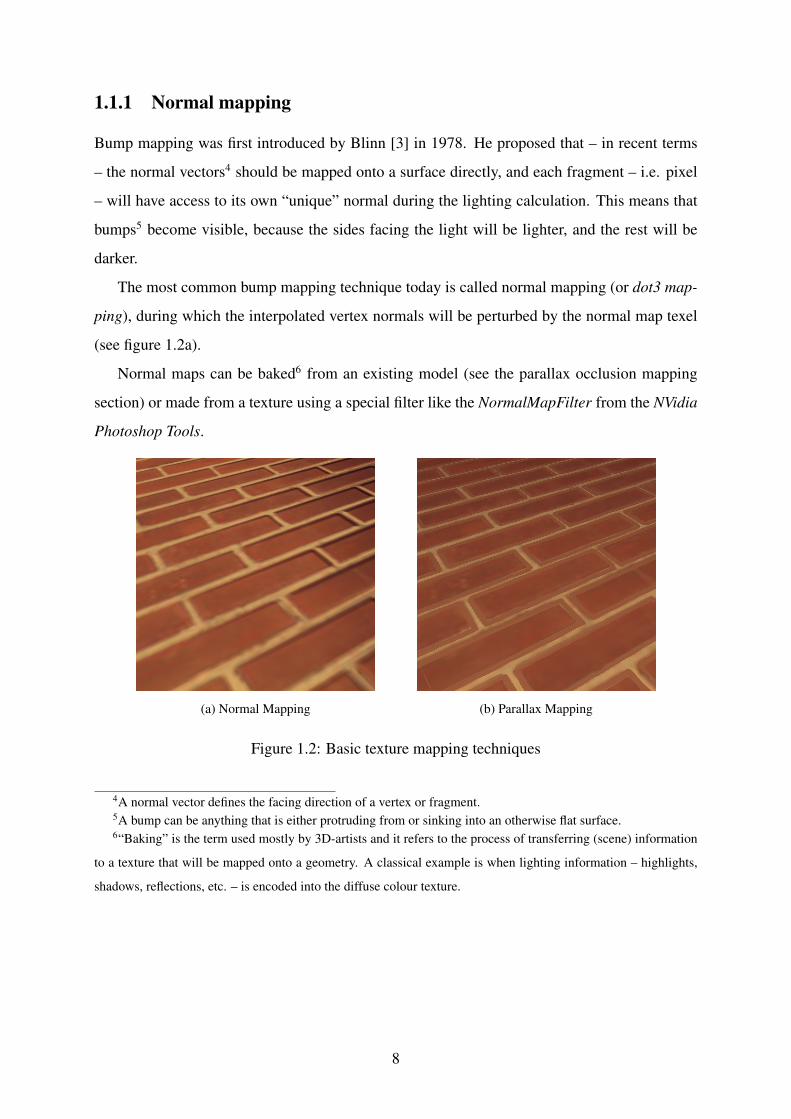
The most common bump mapping technique today is called normal mapping (or dot3 map-

ping), during which the interpolated vertex normals will be perturbed by the normal map texel

(see figure 1.2a).

Normal maps can be baked6 from an existing model (see the parallax occlusion mapping

section) or made from a texture using a special filter like the NormalMapFilter from the NVidia

Photoshop Tools.

(a) Normal Mapping (b) Parallax Mapping

Figure 1.2: Basic texture mapping techniques

4A normal vector defines the facing direction of a vertex or fragment.5A bump can be anything that is either protruding from or sinking into an otherwise flat surface.6“Baking” is the term used mostly by 3D-artists and it refers to the process of transferring (scene) information

to a texture that will be mapped onto a geometry. A classical example is when lighting information – highlights,

shadows, reflections, etc. – is encoded into the diffuse colour texture.

8

1.1.2 Parallax Mapping

Normal mapping improves the render quality a lot, but alone it’s still not convincing enough,

since an important component is missing. That missing piece is the parallax effect7.

The Parallax mapping technique (first introduced by Kaneko [5] and later modified by –

among many – Welsh [10]) accounts for this effect. It’s very simple to implement since only the

displacement of the texture coordinates is needed while taking the view direction and surface-

to-view angle into account, thus achieving some parallax like behaviour.

p = txy + h · vxy (1.1)

The final image (figure 1.2b) looks a lot better now, but Parallax mapping only mimics the

real physical effect. Equation 1.18 will shift the texture coordinates from the view in tangent

space9 without taking into account the self-occlusion. Besides not being physically correct, this

method also have some practical problems, like flattening10 and aliasing11 toward the far edge

of the surface, texture tearing12, etc.

1.2 Parallax Occlusion Mapping

Since normal mapping and parallax mapping cannot simulate true surface depth, a method is

needed that can produce better quality without much real time overhead.

The algorithms that solve this problem are called relief mapping in general. There are many

similar solutions, but here only the most common of these is discussed, which is called Parallax

Occlusion Mapping and was introduced by Tatarchuk ([4]).

7“Parallax is a displacement or difference in the apparent position of an object viewed along two different lines

of sight.” – wikipedia.org8The variables’ meaning here in order are: parallax displacement vector, texture coordinate of the fragment,

height value of the fragment and normalized view direction.9Tangent space is a coordinate system where the fragment is in the origin, while the x (tangent) and y (binormal

or bitangent) axes point toward the direction the texture uv-s increase and z is the fragment normal.10Flattening is the apparent lack of depth at the far end of a parallax surface.11Aliasing is a visual distortion resulting from oversampling. The Moiré effect is one such artefact. The prob-

lem can be avoided if we ensure that the Nyquist criterion is met or can be corrected using filters (this is called

antialiasing).12Tearing is most commonly caused by reading outside the texture’s bounds. It won’t raise segmentation faults

like overreading a buffer does on the CPU side, but some visual artefacts will be visible since no information is

available for the wrongly read texture coordinates.

9

The Parallax Occulsion Mapping – from now on referred to as POM – solves the pre-

cise displacement coordinate calculation by finding the view ray’s intersection point with the

surface height profile (or more accurately the depth profile) while taking self-occlusion and

self-shadowing into account.

This is accomplished by iterating along the view ray and sampling the height texture. Figure

1.3 depicts this process as a diagram showing how to calculate the intersection point.

Figure 1.3: Determining parallax with the height profile

The result is a very good approximation of the real geometry (figure 1.4b), however the

actual quality depends a lot on the sampling rate of course13.

With an inaccurate sampling rate some very obvious visual artefacts (see figure 1.5) will be

visible.

The aliasing (shown a bit later on figure 1.5) is more apparent as we view the surface at

a more grazing angle. To avoid this, increasing the number of samples along the view ray

is necessary. How many samples we need depends on the actual height profile in question.

Practically, we need more samples along the view ray when the surface has deeper and narrower

valleys.

For optimization, I handle the sampling rate in the shader which becomes a function of

the surface-to-view angle and an artist specified value. With taking the angle into account,

the samples will steadily increase while the view-surface angle decreases. The artist specific

13If we have a sample rate that is too low, we might miss the real intersection point. Imagine a peak, that is

ignored because we only sampled before and after it.

10

(a) Without parallax (b) With parallax

Figure 1.4: Parallax Occlusion Mapping

parameter14 is also very important, because some height profiles need more samples and some

require less (as mentioned before).

Aside from that, we should also limit the maximum parallax possible to avoid problems

with texture overreading.

(a) Low sampling rates (b) Higher sampling rates

Figure 1.5: POM aliasing with different sampling rates

In listing 1.1, the HLSL code for finding the parallax displacement is presented. For further

details see [4], [8] and [11].14By artist specific parameter I refer to a value that can be set and adjusted from the outside without modifying

the actual program.

11

1 s t a t i c i n l i n e f l o a t 2 p a r a l l O c l _ 3 _ 0 ( f l o a t 3 tNorm , f l o a t 3 tView , f l o a t 2 uv )2 {3 / / maximum p a r a l l a x o f f s e t ( Welsh )4 f l o a t p a r a l l L i m = l e n g t h ( tView . xy ) / tView . z ∗ matHe iSca l ;56 / / p a r a l l a x v e c t o r ( P )7 f l o a t 2 p a r a l l = n o r m a l i z e (− tView . xy ) ∗ p a r a l l L i m ;89 / / c a l c u l a t e sample r a t e from view a n g l e \ t odo

10 i n t numSamp = para l lSampMin + d o t ( tNorm , tView ) ∗ ( paral lSampMax −para l lSampMin ) ;

11 f l o a t s t e p S z = 1 . 0 f / ( f l o a t ) numSamp ;1213 / / uv−s f o r tex2Dgrad14 f l o a t 2 dx = ddx ( uv ) ;15 f l o a t 2 dy = ddy ( uv ) ;1617 f l o a t viewHei = 1 . 0 ; / / c u r r e n t View h e i g h t ( vh )18 f l o a t 2 u v D e l t a = s t e p S z ∗ p a r a l l ; / / uv s t e p i n P d i r e c t i o n ( d )19 f l o a t 2 currUV = f l o a t 2 ( 0 . 0 f , 0 . 0 f ) ; / / uv a t Pi20 f l o a t 2 prevUV = f l o a t 2 ( 0 . 0 f , 0 . 0 f ) ; / / uv a t P ( i −1)21 f l o a t c u r r H e i ; / / h e i g h t sample a t h i22 f l o a t prevHe i ; / / h e i g h t sample a t h ( i −1)2324 i n t i = 0 ;25 whi le ( i < numSamp )26 {27 / / sample h e i g h t a t i28 f l o a t c u r r H e i = tex2Dgrad ( sampNorm , uv + currUV , dx , dy ) . a ;29 / / i f i n t e r s e c t i o n found30 i f ( c u r r H e i > viewHei )31 {32 / / i n t e r s e c t i o n p o i n t33 / / Pd = ( h ( i −1) − ( vh ( i −1) ) ) / ( d + h i − h ( i −1) )34 f l o a t Pd = ( p revHe i − ( viewHei + s t e p S z ) ) / ( s t e p S z + ( c u r r H e i −

prevHe i ) ) ;35 currUV = prevUV + Pd ∗ u v D e l t a ;36 break ;37 }38 e l s e39 {40 / / i t e r a t e41 viewHei −= s t e p S z ;42 prevUV = currUV ;43 currUV += u v D e l t a ;44 p revHe i = c u r r H e i ;45 ++ i ;46 }47 }4849 re turn uv + currUV ;50 }

Listing 1.1: Parallax displacement function

12

1.3 Self-shadowing

While normal mapping uses precomputed normal vectors which are encoded into the RGBA

texture channels, the (POM) requires the height profile as an additional texture. To save memory

we can combine the two textures into one, because both values are similar in nature and can be

produced at the same time. Usually the height is encoded into the alpha channel and the normal

vector into the R, G and – if used – B channels.

When using POM another very important visual effect can be calculated with the same

resources, namely the self-shadowing. Self-shadowing on a surface occurs, when the light is

blocked by a higher point on the same surface. Because no geometry is available to compute

shadows the usual way – since we want to omit these – it must be done during the parallax

calculation.

Self-shadow calculation fits into the the POM algorithm easily. We can replicate the view

ray sampling from the occluder calculation, but instead of iterating through the view ray, we

sample toward the light source. It’s done by starting at the view-height intersection and moving

along the ray until the height profile is intersected again or the top(1.0 for height maps, 0.0 for

depth maps) is reached. In the first case, the displaced point – which is calculated by POM –

will be in shadow, otherwise it’s lit.

This procedure is illustrated in figure 1.6. The step interval is obtained by multiplying the

“vertical” step value by the normalized tangent space light vector.

1.0

0.0

NL

}1.0 - height

N . L

}number of samples

Figure 1.6: Sampling the during self-occulsion calculation

The main drawback of this approach is, that the resulting shadow will be too “jagged” (figure

1.7a). This can be improved by using Tatarchuk’s method described in [8]. He proposes to use

13

soft shadows and volumetric light sources so shadow penumbras could be calculated, which

eases the transition at the shadow edges – i.e. at the penumbra – making the final result more

appealing.

(a) Aliasing is especially apparent (b) A more appealing shadow

Figure 1.7: Self-occlusion

Moreover, if we look at the surface too closely, than the shadows can stretch unrealistically

far. To solve this, we can use the view angle limitation used by Welsh for the parallax mapping

(see [10]). Other than that, if we decrease the “strength” of the shadowing, we can achieve a

pleasing image similar to figure 1.7b.

1.4 About creating normal and height maps

As mentioned during the normal mapping discussion, normal maps can be generated from

colour channels with a special filter that is available in the NVidia Photoshop Tools plug-in.

However the resulting texture won’t be suitable for every need, since it isn’t being generated

from real geometry.

For the creation of both the normal map and the height map, both the low polygon model

AND the original – high resolution – geometry must be at hand at the same time. Practically

the artist only has to model the higher resolution asset and than reduce the vertices with an

automated mechanism and than adjust the generated mesh manually to achieve satisfactory

result.

With both geometries the normal map can be created easily by sampling the higher res-

olution mesh and than mapping and encoding the normalized normal vectors into a texture.

14

The difference between the fragment normals and the vertex normals can also be stored in the

normal map (both approaches have merits).

For the height map the models must be in the same spatial coordinates. Once this is set up,

the difference between the two meshes can be calculated, thus gaining the raw height values.

Usually the low polygon model is smaller, because it has less detail, so there’s no need to worry

about having negative and positive height values for the same model. Once done with this, we

need to remap the height into the [0.0; 1.0] interval and than store it for example in the normal

map’s alpha channel.

Figure 1.8 shows this set-up in Maya. The green wireframed mesh is the plane the brick

normal and height values will be transferred from the shaded gray geometry.

Figure 1.8: Getting ready for height map baking

When done with this, the textures need to be tested in a rendering environment and adjusted

– scaling and bias parameters – to match our needs. This is especially true for the heigh map,

since it doesn’t store any information about the original bounds of the height profile.

Both the normal and height map generation can be done using a 3D modelling program, like

Autodesk Maya or 3DS Max.

15

Chapter 2

Texture compression

Textures can be used for a lot of things in the GPU pipeline. They can store gloss maps, normal

maps, surface height profile, animation, etc. The primary motivation for using textures is, to

fasten up the rendering process. The very basic use of texture mapping is the application of

color to a triangle’s face. This way, we can avoid building high resolution meshes.

Unfortunately textures can become quite large at some point, and some compromises be-

tween quality and performance must be considered. But we don’t have to necessarily downscale

our images, since we can use compression to reduce the memory load of our assets. However,

we can’t just use any image compression technique we normally would use.

The compression method we require is characterized the following way as described by

Beers et al. in [2]:

• Decoding speed: We need to find a compression method, that is simple enough for us to

be decodable in real time, preferably with the implementation running in the hardware.

So something else is needed than the usual JPEG and similar compressions, because they

require an – for real time rendering – expensive decoding procedure. Basically, we need

a simple enough asynchronous solution.

• Random access: It is quite impossible to predict in which order the texels1 will be ac-

cessed during a run, especially since the programmable pipeline was introduced. This

means, that we need something like a block compression method, where the compressed

texels can be decoded without reading the preceding values.

1A texel is a pixel of a texture. Referring to texture pixels with a different expression is necessary to distinguish

between the fragment pixel – the pixel being rendered – and the texture’s pixel – the pixel being sampled.

16

• Compression rate: We want the best possible performance for the fps-es2 we will need

to sacrifice in order to conserve texture memory and consequently making our application

more dependent on the hardware capabilities (the developer cannot assume that his/her

chosen compression method will be supported “out-of-the-box”).

• Compression quality: Since the other criteria don’t leave much room for lossless com-

pression methods, it must be ensure that the amount of quality degradation is acceptable.

Beers et al. included the encoding speed in their list too, but in our particular application we

only consider offline compression. In video game development it can be said, that prerendering

– or baking – as much as possible during the development process is widely accepted policy.

In the following sections we will look at some popular compression techniques available on

current hardware.

2.1 DXTn compression

These compression methods ware developed by S3 Graphics, Ltd. during the ’90s and they are

the most widespread and supported compression techniques available yet. DXTn is also called

S3TC or DXTC3 sometimes.

The name refers to a family of similar compression models that use 4 × 4 kernels. The

compression ratio – depending on the version – is between 6:1 and 4:14 and they can be used

for both RGB and RGBA texture formats5.

The compressed pixels are stored in two 16-bit values followed by four code bytes6. The

codes specify how to mix the two colour values to recreate the original values in a given block.

Here every 2 bits represent a pixel and can be used to reconstruct the pixel colour (see table

2.1).

There are a number of DXTn compressions. There isn’t a choice that suites every need, so

we should consider how each would fit into a given scenario. The following list describes the

more popular and therefore most supported versions.2The frame per second is a measurement quantity which specifies how many time the screen was refreshed in

a second. Usually we need 24 frames for each second to convey continuous motion on the screen, but 60 is the

standard in video gaming (especially for fast paced games like racing games and shooters).3It’s called DXTC because of their early incorporation into DirectX.4Meaning the compressed image will be 4 or 6 times smaller than the uncompressed one.5A denotes the alpha channel, which is usually used for storing transparency values.6At least, this is the case for DXT1, but the other variations are quite similar too.

17

code colour0 > colour1 colour0 ≤ colour1

0 colour0 colour0

1 colour1 colour1

22·colour0+colour1

3colour0+colour1

2

3colour0+2·colour1

3 Black

Table 2.1: Interpretation of DXT1 codes

• DXT1 This compression version only supports the RGB 565 scheme (5 bits red, 6 bits

green and 5 bits blue). This one has the best compression ratio of 6:1 (among DXTn), but

with the obvious drawback of having only three channels.

• DXT3 The third version is the same as the first one, except that it adds a 4-bit, uninterpo-

lated alpha channel to the compression. This compression has a 4:1 ratio.

• DXT5 This in the only variant which supports the entire 4 channel compression with 8-

bit alpha representation and a 3-bit interpolation factor. The compression benefits are the

same as in DXT3.

On figures 2.1c and 2.1d we can see the DXTn compression. Compared to the original

texture (fig. 2.1a), we can clearly identify the pixel groups. Also, we can notice, that DXT5

preserved more detail than DXT1 thanks to the better precision it has. I also noticed a minor

decrease in fillrate, when compressed textures ware used, but it’s barely noticeable.

In practice, the textures can be compressed using the NVidia Photoshop Tools which adds

support for DSS file format. The DSS stands for Direct Draw Surface and is originally was

intended to be used in DirectX. It’s capable of storing compressed textures in the DXTn format

and also supports mip map levels. The file format itself is very simple and we can implement a

loading mechanism for OpenGL fairly easily.

Once we have the texture date loaded, we can use glCompressedTexImage2D() to

upload it to the graphical memory. For this to work, the OpenGL driver has to support the

EXT_texture_compression_s3tc extention. This is usually available, but we should check re-

gardless7.

7In my experience, the COMPRESSED_RGBA_S3TC_DXT5_EXT parameter for the

glCompressedTexImage2D() call wasn’t available in the native Android header, but once manually

18

(a) Bitmap (b) ETC1

(c) DXT1 (d) DXT5

Figure 2.1: Compression methods

19

2.2 ATI compression

In my opinion DXT5 is perfect for any need because it supports all of the channels and has

a good compression ratio, however normal map compression can be error prone, since we can

lose a lot of surface curvature information. This is due the usage of the 4×4 kernel, which mixes

16 pixels into one. Normally we can detect such loss in an RBG image, but normal maps are

treated differently, because we the values can be drastically different depending on the surface’s

divergence like the one on figure 2.2a8. It’s not hard to see, how compressing such normal map

would affect the result. Figure 2.2d clearly shows how DXT1 fails in this case.

A good solution is to use ATI29 compression. This method compresses two channels based

on DXT5. It is able to interpolate between 8 values per channel. In the case of normal mapping,

2 of the 3 components are enough for us, since the third can be derived on the fly using equation

2.110. ATI1 and ATI2 ware originally only available on ATI/AMD chips and Direct3D 10.0+

hardware, but it became on open standard and is available as an extention for most OpenGL

versions11.

nz =√

1− n2x − n2

y (2.1)

Take a look at figures 2.2c and 2.2e. The difference in quality is evident. With a 32-bit

precision ATI2 compression can compress up to 1:2 rate12.

If this compression method isn’t supported on our hardware a common fallback method is

to use DXT5’s green and alpha channel, since these have the highest precision possible.

AMD provides a compression tool called TheCompressonator which can compress texture

in both ATI1 and ATI2 among many others. The non-thresholded versions of the difference

images show on figures 2.2c and 2.2e ware also made by this tool.

declared – 0x83F3 – it worked without further problems.8The illustration only shows only 1/4 part of the original normal map since we wouldn’t be able to see much in

this size.9ATI1 supports compression for only one channel.

10This is only possible because the z for a normal is always positive – i.e. point outward for a face.11It is also called BC5 or 3Dc.12While ATI1’s compression rate is 1:4.

20

(a) The uncompressed normal map (b) Uncompressed normal mapping

(c) Thresholded DXT1 difference (d) DXT1 compressed normal mapping

(e) Thresholded ATI2 difference (f) ATI2 compressed normal mapping

Figure 2.2: Normal map compression comparison

21

2.3 ETC compression

The Ericsson Texture Compression – abbreviated as ETC – is another compression scheme

that is available on portable devices. The ETC compression has two versions. ETC1 can only

compress RGB channels while ETC2 can compress the alpha too. This method is part of the

OpenGL ES 3.0 standard and is included in the Android platform since version 2.0 to comple-

ment it’s absence in OpenGL 1.0 and 2.0.

The ETC1 compression compresses using 4×4 blocks, which are divided into two 4×2 or

2×4 chunks13. Than both chunk’s pixels are assigned the same colour or an 3-bit offset from a

common base colour14. Also, each half has a brightness property which is stored in a separate

lookup table. Finally, each chunk is offsetted from the block’s base colour.

The ETC1 compression has a 1:6 ration same as DXT1 and produces better image quality

– compare figures 2.1c and 2.1b – but takes longer to decompress because it uses up more

bandwidth.

13The choice here is made for the one that produces better compression ratio.14Again, the decision is made for the best performance.

22

Chapter 3

Fluid Simulation

Big part of video games revolves around the interaction with a virtual environment in real time.

These interactions can range from simply picking up objects from the ground to physically

influencing the environment the player is presented with (for example gravity). Of course sim-

ulating physics is more interesting and more challenging. In some cases the interaction with the

physical environment can be precalculated and activated when needed. Unfortunately always

relying on this method is not possible and some degree of simulation is at some point needed.

Some physical calculations can be calculated in parallel to benefit from implementation on

the GPU. NVidia’s PhysiX SDK uses the power of the graphical processing pipeline for this

exact purpose, however it is only available on NVidia GPU-s and on computers with greater

performance than portable devices can offer. Therefore a specialized solution would be benefi-

cial .

In this text I’ve chosen fluid simulation to be discussed here since it relies heavily on the

GPU rendering pipeline, and can be used to simulate not only “water like” substances, but also

smoke, clouds and similar substances.

3.1 The Navier-Stokes equations

The development of mathematical fluid simulations can be traced back to the 19th century and

ware refined by scientists until they reached their current form. The Navier-Stokes equations are

one of these1 and can be used to accurately calculate the flow of fluids. The whole expression

1Other fluid simulation techniques include for example the Lattice Boltzmann methods and Smoothed-particle

hydrodynamics

23

is given in equation 3.1:

∂u

∂t= − (u · ∇)u− 1

ρ∇p+ v∇2u+ f (3.1)

This solution can be broken down into four parts: advection, pressure, diffusion and force

or forces that change the state of the fluid.

Advection

− (u · ∇)u (3.2)

deals with the motions of fluid like substances. It can be applied to any quantity and is repre-

sented by a vector field.

Pressure

−1

ρ∇p (3.3)

influences how the molecules in the fluid behave by altering the velocity field.

Diffusion

v∇2u (3.4)

describes how fluids with different densities exchange and mix their masses. Viscosity is the

name for the fluid’s resistance to flows and is connected to the diffusion.

Forces – f – alter the way the fluid will evolve and is required for making the fluid simulation

interactive.

In the following sections discuss the general approach to fluid simulation using the GPU.

3.2 Water in a buffer

Analytically solving equation 3.1 on the GPU is not practical, therefore a numerical method is

needed which can iteratively evaluate it. The presentation of the numerical approach is out of

the scope of this work. For the application it is sufficient to know that the original equation can

be rewritten in the following manner using the Helmholtz-Hodge decomposition:

S(u) = A · F · D · P(u) (3.5)

Using equation 3.5 it’s possible to calculate the advection (A), diffusion (D), projection (P)

and the addition of forces (F) separately and evaluate them all for the final state in a given time

24

frame. The projection part is a new element, which is used to ensure that the fluid acts in a mass

conserving way. For an in depth discussion see [6].

The shader implementation heavily uses the render-to-texture technique (in Direct3D terms

render targets, or in OpenGL the Frame Buffer Objects – FBO). In every step, the buffers are

rendered into a texture which will be uploaded to the graphical memory for the next shader.

Since FBO-s can only represent values between 0.0 and 1.0, they should be scaled into this

range (this means that 0.0 is interpreted as −1.0 and 0.5 as 0.0, and so on).

3.3 Shader solution

The general solution presented here is based on the slides from “GPU általános célú pro-

gramozása” ([9]), a course about general GPU programming. I used the original OpenCL

implementation presented during the classes as a basis for my GLSL solution.

The first step in the implementation is the addition of forces that occurred between the last

time step and the present time. This step is self evident and is show in listing 3.1.

1 void main ( )2 {3 / / read c u r r e n t v a l u e s4 vec4 v e l o c i t y D i v e r g e n c e V a l = t e x t u r e 2 D ( u_ve loc i t yDive rgenceBufSamp ,

v_ texCoord ) ;5 v e l o c i t y D i v e r g e n c e V a l = v e l o c i t y D i v e r g e n c e V a l ∗ 2 . 0 − 1 . 0 ;67 / / add f o r c e8 vec2 d = u _ t o u c h P o s i t i o n − v_texCoord ;9 f l o a t a r e a = exp (− ( ( d . x ∗ d . x + d . y ∗ d . y ) ∗ RADIUS) ) ;

10 v e l o c i t y D i v e r g e n c e V a l . xy =11 ( v e l o c i t y D i v e r g e n c e V a l . xy + a r e a ∗ u _ o r i e n t a t i o n . xy ∗ u _ t o u c h D e l t a ) ;1213 / / o u t14 v e l o c i t y D i v e r g e n c e V a l = ( v e l o c i t y D i v e r g e n c e V a l + 1 . 0 ) / 2 . 0 ;15 g l _ F r a g C o l o r = vec4 ( v e l o c i t y D i v e r g e n c e V a l . xyz , 1 . 0 ) ;16 }

Listing 3.1: Addition of forces

This solution uses a velocity and a density buffer. The example adds a circularly shaped

force pattern to the velocity buffer. The same applies for the density buffer. It is important to

properly initialize the buffers before first accessing them.

Once the new forces have been added, the advection shader can be run (3.2).

This backtraces the velocity value to its original coordinate and calculates the new veloc-

ity value from the incoming and outgoing vectors by applying a bilinear interpolation to the

25

1 void main ( )2 {3 / / read v a l u e s w i t h new f o r c e s added4 vec4 v e l o c i t y D i v e r g e n c e V a l = t e x t u r e 2 D ( u_ve loc i t yDive rgenceBufSamp ,

v_ texCoord ) ;5 v e l o c i t y D i v e r g e n c e V a l = v e l o c i t y D i v e r g e n c e V a l ∗ 2 . 0 − 1 . 0 ;67 / / c a l c u l a t e t h e v e l o c i t y d i s p l a c e m e n t8 vec2 p ;9 p . x = v_ texCoord . x − u _ t i m e D e l t a ∗ v e l o c i t y D i v e r g e n c e V a l . x ;

10 p . y = v_ texCoord . y − u _ t i m e D e l t a ∗ v e l o c i t y D i v e r g e n c e V a l . y ;1112 / / c a l c u l a t e t h e new v e l o c i t y v a l u e13 g l _ F r a g C o l o r = vec4 ( t e x t u r e 2 D B i l i n e a r ( p ) , v e l o c i t y D i v e r g e n c e V a l . zw ) ;14 }

Listing 3.2: Advection of velocities

surrounding texels. It is analogous for the density buffer.

The next step is the diffusion. Listing 3.3 shows how to account for the viscosity – or the

“spreading out” – of a fluid. A lower viscosity would make the fluid act as a thin water, a higher

value would mean something like honey.

Next the pressure is calculated. This requires having the divergence calculated and available

before solving the numerical solution to calculate the final pressure value. In this case, the Ja-

cobi iteration is used. Since it’s iterative, the more time it’s applied with running this particular

shader, the more accurate are the results. Experiments have shown that 5 to 10 iterations are

required to have good results and acceptable performance on a Blackberry Playbook. Since

the code for these two shaders only slightly differ from the viscosity calculation and are not

very interesting in our discussion, they’ll be omit here. See the slides from [9] for the OpenCL

implementation.

Lastly the projection (3.4) is used, which makes the fluid mass conserving and divergence

free.

This concludes the discussion about the general approach for the Navier-Stokes equations.

Figure 3.1 shows the buffers in action. In this example three different fluidswhich have opposite

velocities are colliding (as seen on fig. 3.1a). On figure 3.1b we can see that most of the pres-

sure is concentrated along the collision lines and the space between the main flows, basically

compressing the middle areas together. The 3.1c buffer is used for the pressure calculations and

the collision lines can be clearly identified in it.

The images from 3.1 were taken on a Blackberry Playbook with a buffer size of 800p×800p

and 10 Jacobi iterations. Although this implementations is capable of running in real time on

26

(a) Velocity buffer

(b) Pressure buffer (c) Divergence buffer

Figure 3.1: Buffers

27

1 void main ( )2 {3 / / read c u r r e n t b u f f e r4 vec4 v e l o c i t y D i v e r g e n c e V a l = t e x t u r e 2 D ( u_ve loc i t yDive rgenceBufSamp ,

v_ texCoord ) ;5 v e l o c i t y D i v e r g e n c e V a l = v e l o c i t y D i v e r g e n c e V a l ∗ 2 . 0 − 1 . 0 ;67 / / s e t up t h e v i s c o s i t y8 f l o a t a l p h a = 1 . 0 / v i s c o s i t y ;9 f l o a t b e t a = 1 . 0 / ( 4 . 0 + a l p h a ) ;

1011 / / sample t h e n e i g h b o u r i n g c e l l s12 vec2 vL = t e x t u r e 2 D ( u_ve loc i t yDive rgenceBufSamp ,13 vec2 ( v_ texCoord . x − u _ s t e p S z . x , v_ texCoord . y ) ) . xy ;14 vec2 vR = t e x t u r e 2 D ( u_ve loc i t yDive rgenceBufSamp ,15 vec2 ( v_ texCoord . x + u _ s t e p S z . x , v_ texCoord . y ) ) . xy ;16 vec2 vB = t e x t u r e 2 D ( u_ve loc i t yDive rgenceBufSamp ,17 vec2 ( v_ texCoord . x , v_ texCoord . y − u _ s t e p S z . y ) ) . xy ;18 vec2 vT = t e x t u r e 2 D ( u_ve loc i t yDive rgenceBufSamp ,19 vec2 ( v_ texCoord . x , v_ texCoord . y + u _ s t e p S z . y ) ) . xy ;2021 / / a p p l y t h e v i s c o s i t y22 v e l o c i t y D i v e r g e n c e V a l . xy = ( vL + vR + vB + vT + a l p h a23 ∗ v e l o c i t y D i v e r g e n c e V a l . xy ) ∗ b e t a ;2425 / / o u t26 v e l o c i t y D i v e r g e n c e V a l = ( v e l o c i t y D i v e r g e n c e V a l + 1 . 0 ) / 2 . 0 ;27 g l _ F r a g C o l o r = vec4 ( v e l o c i t y D i v e r g e n c e V a l . xyz , 1 . 0 ) ;28 }

Listing 3.3: Viscosity calculation

1 void main ( )2 {3 / / read b u f f e r4 vec4 v e l o c i t y D i v e r g e n c e V a l = t e x t u r e 2 D ( u_ve loc i t yDive rgenceBufSamp ,

v_ texCoord ) ;5 v e l o c i t y D i v e r g e n c e V a l = v e l o c i t y D i v e r g e n c e V a l ∗ 2 . 0 − 1 . 0 ;67 / / sample ne ighbour s , f o r b r e v i t y some p a r t s are o m i t t e d8 f l o a t pL = t e x t u r e 2 D ( u _ d e n s i t y P r e s s u r e B u f S a m p , . . .9 f l o a t pR = t e x t u r e 2 D ( u _ d e n s i t y P r e s s u r e B u f S a m p , . . .

10 f l o a t pB = t e x t u r e 2 D ( u _ d e n s i t y P r e s s u r e B u f S a m p , . . .11 f l o a t pT = t e x t u r e 2 D ( u _ d e n s i t y P r e s s u r e B u f S a m p , . . .1213 / / a p p l y p r o j e c t i o n14 v e l o c i t y D i v e r g e n c e V a l . xy = v e l o c i t y D i v e r g e n c e V a l . xy − vec2 ( pR − pL , pT

− pB ) ;1516 / / o u t17 v e l o c i t y D i v e r g e n c e V a l = ( v e l o c i t y D i v e r g e n c e V a l + 1 . 0 ) / 2 . 0 ;18 g l _ F r a g C o l o r = vec4 ( v e l o c i t y D i v e r g e n c e V a l . xyz , 1 . 0 ) ;19 }

Listing 3.4: Applying the projection

28

this device, it should be adjusted for use in games. This solution can be easily combined with

existing assets – like height texture, where high values act as a constant 0 velocity which cannot

be move by the fields.

Also as a last note: in the shader codes presented here the boundary conditions ware omitted

for the sake of brevity but they can be handled with ease. For a more in depth presentation of

Navier-Stokes fluid simulation for game see [7].

29

Bibliography

[1] Thomas Akenine-Möller, Eric Haines, and Naty Hoffman. Real-Time Rendering. A K

Peters, Ltd., 3rd edition, 2008.

[2] Andrew C. Beers, Maneesh Agrawala, and Navin Chaddha. Rendering from compressed

textures. In Proceedings of the 23rd annual conference on Computer graphics and inter-

active techniques, SIGGRAPH ’96, pages 373–378, New York, NY, USA, 1996. ACM.

[3] James F. Blinn. Simulation of wrinkled surfaces. 1978.

[4] Zoe Brawley and Natalya Tatarchuk. Parallax occlusion mapping: Self-shadowing,

perspective-correct bump mapping using reverse height map tracing. ShaderX3: Advanced

Rendering with DirectX and OpenGL, 2004.

[5] Tomomichi Kaneko, Toshiyuki Takahei, Masahiko Inami, Naoki Kawakami, Yasuyuki

Yanagida, Taro Maeda, and Susumu Tachi. Detailed shape representation with parallax

mapping. In In Proceedings of the ICAT 2001, pages 205–208, 2001.

[6] Jos Stam. Stable fluids. In Proceedings of the 26th annual conference on Computer

graphics and interactive techniques, SIGGRAPH ’99, pages 121–128, New York, NY,

USA, 1999. ACM Press/Addison-Wesley Publishing Co.

[7] Jos Stam. Real-time fluid dynamics for games, 2003.

[8] Natalya Tatarchuk. Practical parallax occlusion mapping for highly detailed surface ren-

dering. In SIGGRAPH2006, 2006.

[9] Balázs Tóth, Szirmay-Kalos László, and Szécsi László. Gpu általános célú programozása

(gpgpu) - folyadék szimuláció, okt 2012.

[10] Terry Welsh. Parallax mapping with offset limiting: A perpixel approximation of uneven

surfaces. 2004.

30

[11] Jason Zink. A closer look at parallax occlusion mapping, jun 2006.

31